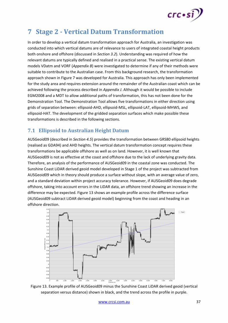
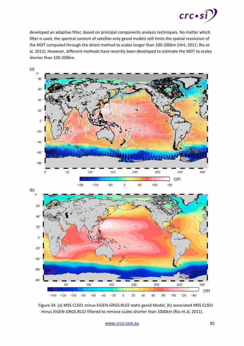
www.crcsi.com.au Vertical Datum Transformations across the Littoral Zone Developing a method to establish a common vertical datum before integrating land height data with near‐ shore seafloor depth data J.H. Keysers, N.D. Quadros and P.A. Collier Report prepared for the Commonwealth Government of Australia, Department of Climate Change and Energy Efficiency
Appendix C ‐ Australian Tide Gauge Data ................................................................................... 90
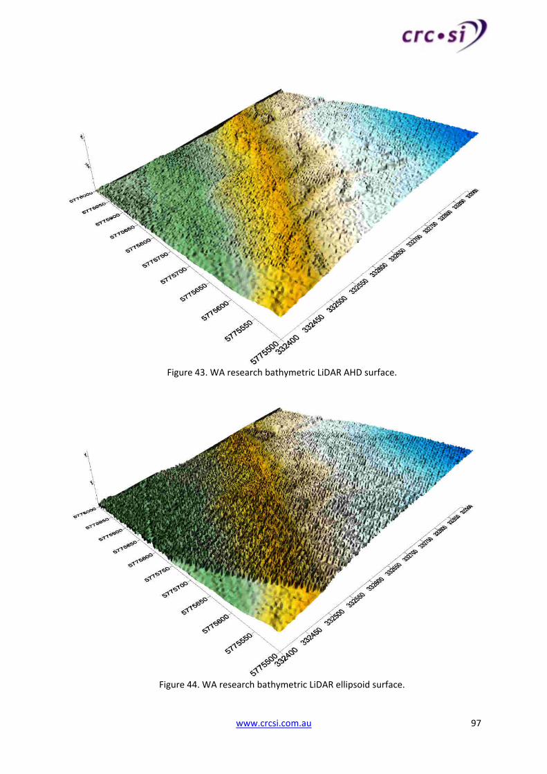
Appendix D ‐ Stage 1 LiDAR Analysis .......................................................................................... 96
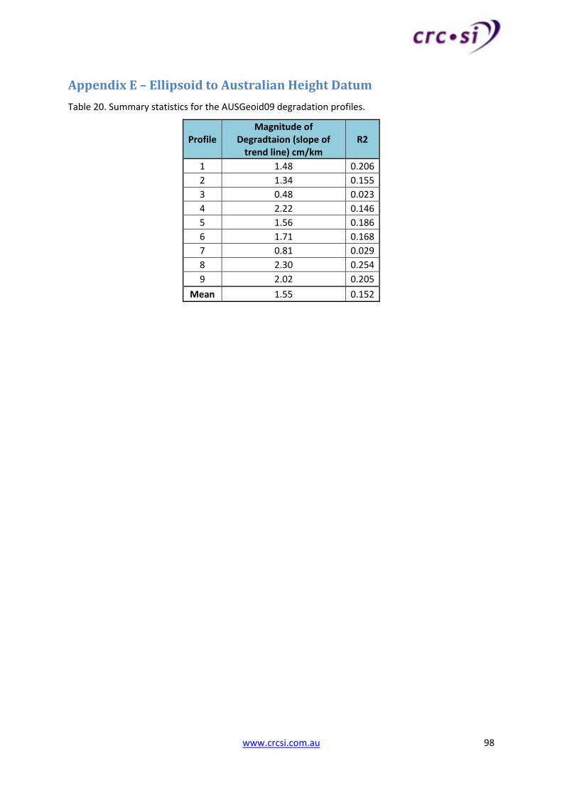
Appendix E – Ellipsoid to Australian Height Datum ................................................................... 98
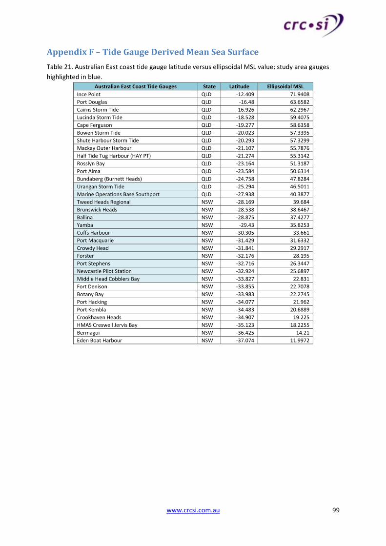
Appendix F – Tide Gauge Derived Mean Sea Surface ................................................................ 99
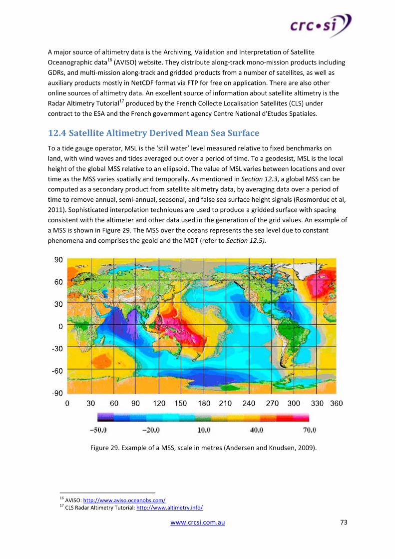
Appendix G – Satellite Altimetry Derived Mean Sea Surface ................................................... 101
Appendix H – Integrated Mean Sea Surface............................................................................. 103
Appendix I – GEMS ................................................................................................................... 104
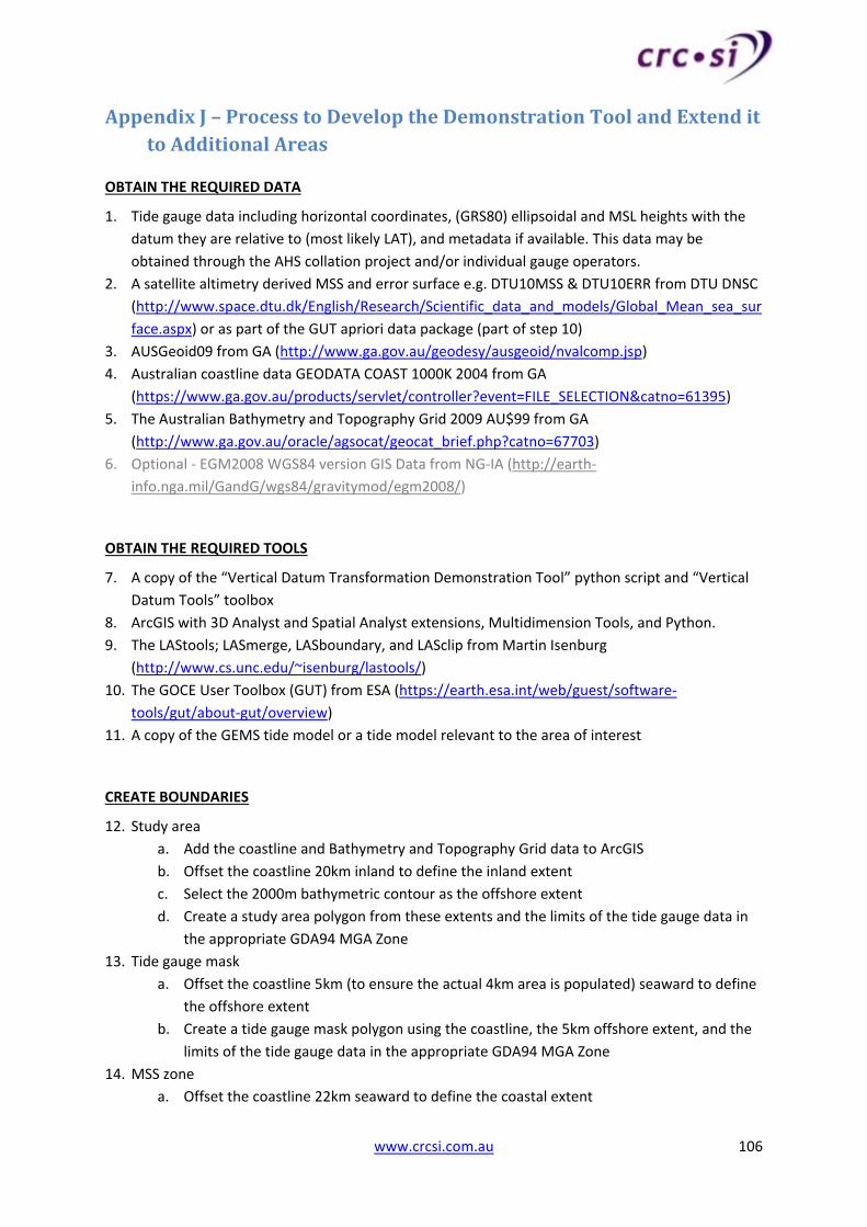
Appendix J – Process to Develop the Demonstration Tool and Extend it to Additional Areas 106
www.crcsi.com.au 8
AcknowledgementsThe authors wish to acknowledge that this report was funded by the Government of Australia through the Department of Climate Change and Energy Efficiency as part of Phase two of the Urban Digital Elevation Modelling (UDEM2) project. The authors wish to thank the following people and organisations for providing advice, data and tools to the project;
‐ Zarina Jayaswal, Australian Hydrographic Service (AHS)
‐ Nicholas Dando and Nicholas Brown, Geoscience Australia (GA)
‐ G. John Broadbent, Queensland Climate Change Centre of Excellence (QCCCE)
‐ Bill Mitchell and James Chittleborough, Bureau of Meteorology National Tidal Centre (NTC)
‐ Edward Myers, VDatum Project, National Oceanic and Atmospheric Administration (NOAA)
United States
‐ Ole Anderson, Danish Technical University (DTU) Danish National Space Centre (DNSC)
‐ Marek Ziebart, VORF, University College London (UCL)
‐ Salvatore Dinardo, European Space Agency (ESA)
‐ Michael Kuhn, Curtin University
‐ Martin Isenburg, LAStools
‐ Michael Conroy, Rick Frisina, and Christina Ratcliff, Department of Sustainability and
Environment (DSE), Victoria.
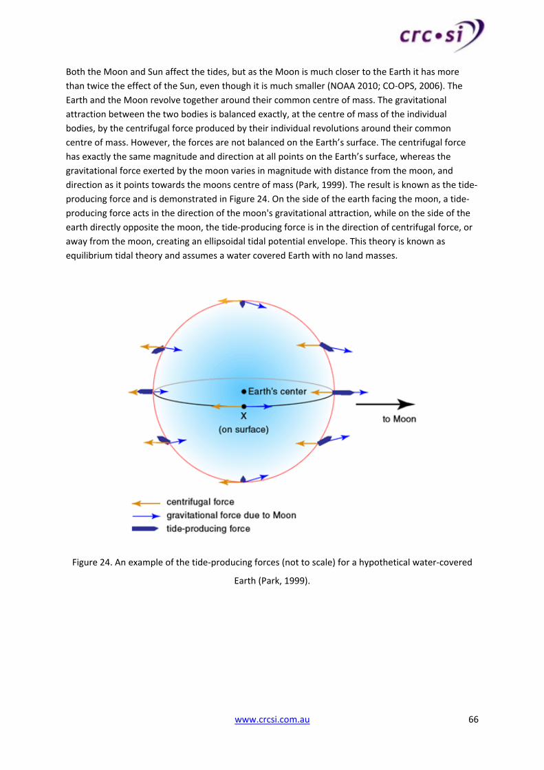
‐ David Provis, Oceanographer, Cardno
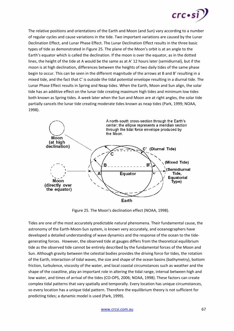
‐ Neil White, Commonwealth Scientific and Industrial Research Organisation (CSIRO), Australia
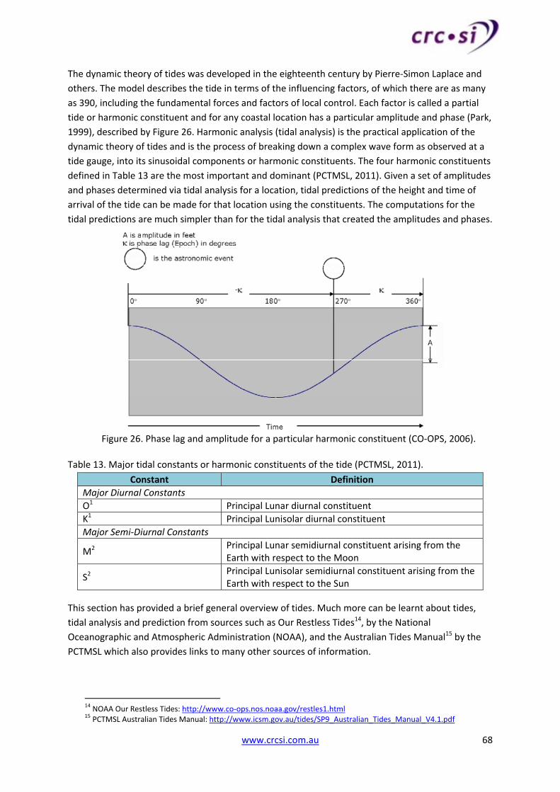
‐ Peter Todd, Senior Survey Advisor, Geodesy & Positioning, Queensland Government
(formerly DERM)
‐ Dr. Graeme Hubbert, GEMS
Acknowledgments also extend to Fugro Spatial, Fugro LADS, Photomapping Services, Schlencker
Mapping Pty Ltd, and Archiving, Validation and Interpretation of Satellite Oceanographic data
(AVISO) for providing data used as part of the project.
www.crcsi.com.au 9
ListofacronymsAHD Australian Height Datum
AHS Australian Hydrographic Service
AMSA Australian Maritime Safety Authority
ANTT Australian National Tide Tables
ATT Admiralty Tide Tables (UK)
AVISO Archiving, Validation and Interpretation of Satellite Oceanographic data
BoM Bureau of Meteorology
CD Chart Datum
CLS Collecte Localisation Satellites (France)
CO‐OPS Center for Operational Oceanographic Products and Services (US)
CRCSI Cooperative Research Centre for Spatial Information
DEM Digital Elevation Model
DNSC Danish National Space Centre
DT Dynamic Topography
DTU Danish Technical University
EGM2008 Earth Gravitational Model 2008
ESA European Space Agency
ESRI Environmental Systems Research Institute
ETRF89 European Terrestrial Reference Frame 1989
GA Geoscience Australia
GDA94 Geocentric Datum of Australia 1994
GDR Geophysical Data Record
GEMS Global Environmental Modelling Solutions
GIS Geographic Information System
GNSS Global Navigation Satellite System
GRS80 Geodetic Reference System 1980
HAT Highest Astronomical Tide
ICSM Intergovernmental Committee on Surveying and Mapping
IHO International Hydrographic Organization
ITRF International Terrestrial Reference Frame
LAS Common LiDAR Data Exchange Format
LAT Lowest Astronomical Tide
LiDAR Light Detection and Ranging LMSL Local Mean Sea Level (US)
MDT Mean Dynamic Topography
MGA Map Grid of Australia
MHW Mean High Water
MHWS Mean High Water Springs
MLW Mean Low Water
MLLW Mean Lower Low Water (US)
MLWS Mean Low Water Springs
MSL Mean Sea Level
MSQ Maritime Safety Queensland
www.crcsi.com.au 10
MSS Mean Sea Surface
NAD83 North American Datum 1983
NAVD88 North American Vertical Datum 1988
NEDF National Elevation Data Framework
NGS National Geodetic Survey (US)
NIB/IB No Inverse Barometer/Inverse Barometer
NOAA National Oceanographic and Atmospheric Administration (US)
NTC National Tidal Centre
NTDE National Tidal Datum Epoch
OSGM05 Ordnance Survey Gravity Model 2005 (UK)
PCTMSL Permanent Committee on Tides and Mean Sea Level
POL Proudman Oceanographic Laboratory (UK)
PSMSL Permanent Service for Mean Sea Level (global)
QCCCE Queensland Climate Change Centre of Excellence
SLA Sea Level Anomaly
SST Sea Surface Topography
TCARI Tidal Constituent And Residual Interpolation (US)
TIN Triangulated Irregular Network
TSS Topography of the Sea Surface
UCL University College London
UKHO United Kingdom Hydrographic Office
UK United Kingdom
US United States of America
VDatum Vertical Datum Transformation (US)
VORF Vertical Offshore Reference Frame (UK)
WA Western Australia
WGS84 World Geodetic System 1984
www.crcsi.com.au 11
1 Introduction
1.1 Rationale
Australia’s coastal zone is of great economic, social and environmental importance. Around 85 per
cent of the population live in the coastal zone (DCCEE, 2009). This area is vulnerable to the projected
impacts of climate change, creating a demand for better information to assess the risks associated
with sea‐level rise and coastal inundation.
High accuracy topographic data currently allows simple “bathtub” modelling of sea level rise
wherein a location is inundated if its elevation is less than or equal to the projected sea level,
regardless of hydrological considerations. The inclusion of high accuracy bathymetric data and the
creation of seamless coastal datasets will provide coastal modellers with the ability to consider the
hydrological connectivity of the land to the sea and hence model coastal inundation more
accurately. The assessment of coastal risks, and the development of effective adaptation and
mitigation strategies requires seamless elevation models with a vertical accuracy of better than 0.5m
and a horizontal resolution of better than 1 second of arc (30m) (ANZLIC, 2008).
Seamless coastal data products necessitate the integration of topographic height data with
bathymetric depth data. Elevation data free of discontinuities, where topography and bathymetry
merge, is necessary to accurately model coastal processes. For such high resolution, high accuracy
applications, a pre‐requisite for the integration process is that the respective elevation datasets be
related to the same vertical datum. By establishing a common vertical datum prior to integration,
the major source of systematic error is removed. Applications with low accuracy requirements may
not require the establishment of a common vertical datum however this project arose out of the
National Elevation Data Framework (NEDF) project. For the NEDF, vertical datums were identified as
a research issue to be addressed to facilitate the development of a high resolution national DEM
with integrated topography and bathymetry (ANZLIC, 2008). The development of such a DEM is also
driven by the National Climate Change Adaptation Framework (COAG, 2007).
Traditionally, the hydrographic and topographic communities have operated independently. This has
resulted in bathymetric and topographic data being used autonomously and referenced to different
vertical datums. Topographic height datasets can be classified into two types of reference systems:
Geometric height systems ‐ Not related to the Earth’s gravity field (i.e. ellipsoidal systems
useful for example in monitoring crustal movement and airborne mapping); and
Physical/natural height systems ‐ Related to the Earth’s gravitational field or geoid (e.g. the
Australian Height Datum (AHD) which can be used to predict and measure direction and rate
of fluid flow amongst other practical applications) (Featherstone, 2006).
In the marine environment, the situation is more complex, with a wider variety of vertical datums
being used. Depth measurements are related to tidal datums such as Lowest Astronomical Tide (LAT)
or Mean Sea Level (MSL) and primarily support safe navigation but are also the basis for establishing
cadastral and maritime boundaries. Chart Datums are employed for the production of hydrographic
www.crcsi.com.au 12
charts. Many hydrographic surveyors are now also using the ellipsoid for vertical positioning (Dodd
et al, 2010).
In recent years, the use of bathymetric data has moved beyond navigation charts, towards
supporting coastal zone management applications (Dodd et al, 2010; Parker, 2002). A number of
these applications require a continuous, seamless elevation dataset across the land/sea interface.
According to a survey conducted in recent research by Quadros et al (2012), 65% of Australian
bathymetry users require the integration of bathymetric and topographic data for applications such
as storm surge modelling and coastal inundation assessments. Hence there has been a growing
investment in near‐shore bathymetric and topographic Light Detection and Ranging (LiDAR) surveys
around Australia which has led to the development of seamless digital elevation models (DEMs)
spanning the land‐sea interface. There has been difficulty in the production of these DEMs without a
method for establishing a common vertical datum. LiDAR technology is able to provide near‐shore
depth data, in areas inaccessible to surface vessels.
The applications benefitting from a seamless coastal elevation dataset include, but are not limited
to: studying the impacts of sea level rise, storm surge inundation modelling, tsunami inundation
modelling, coastal zone management, marine boundary delimitation, habitat restoration, erosion
studies, coastal ecosystem modelling, beach renourishment projects, coastal construction and
development, shoreline change analysis, improved efficiency of hydrographic surveying by reducing
the reliance on tide gauges and tidal models, and building and maintaining the national DEM.
Given the use of different vertical datums for height and depth data, integrating topographic and
bathymetric datasets across the coastal zone has been and continues to be problematic. Australian
bathymetry users have identified vertical datums as one of the most common problems experienced
in this context (Quadros et al, 2012). The problem has also been highlighted in projects such as the
development of the Victorian coastal DEM (Quadros and Collier, 2009). There is increasing need and
demand for a system to efficiently transform elevations between all the relevant vertical reference
surfaces. To achieve this, the relationships between the relevant vertical reference frames need to
be determined, modelled and applied. Due to the localised nature of the geometric and temporal
variations in tidal datums this is not a straightforward task. Tidal datum surfaces are notoriously
difficult to realise in practice because of the temporal and spatial variations they experience and the
requirement for long period observation (NOAA, 2007; CO‐OPS, 2006).
This project focused on adopting an ellipsoid‐based approach for vertical datum transformations of
coastal zone elevation data. The ellipsoid is the only surface that is used for modern data collection
on both land and sea (Dodd et al, 2010). Traditionally, reference ellipsoids were used to define
horizontal datums but with the emergence of high‐accuracy Global Navigation Satellite System
(GNSS), reference ellipsoids are now also being used to define vertical datums. The GNSS provides
accurate, repeatable and cost‐effective ellipsoid heights at tide gauges and bench marks which
enable ellipsoid‐based transformations. While not of particular practical value to many users, an
ellipsoidal height datum can be rigorously defined and realised in a repeatable manner. This
temporal and geometric stability yields a consistent frame of reference for the purposes of
developing transformation models.
www.crcsi.com.au 13
The International Federation of Surveyors (FIG, 2006) suggested the Geodetic Reference System
1980 (GRS80) ellipsoid as a suitable base for inter‐relating vertical reference surfaces for
hydrographic purposes. International projects (discussed in Section 3 & Appendix B) also tend to
adopt ellipsoid‐based approaches. Given there is an intention to move Australia to a dynamic version
of GDA in 2020 with the associated ellipsoidal height datum replacing AHD as the national height
reference surface (Dando, 2012) an ellipsoid‐based approach is justified. While such an approach is
conceptually simple, technically sound and eminently logical, implementation on a national scale is
complex and time consuming.
The vertical datum transformation approach and recommendations of this project aim to enable the
creation of seamless elevation datasets across the littoral zone, being the zone between the highest
and lowest tidal lines. The Demonstration Tool developed for the study area transforms elevation
data between a number of common vertical datums. This enables adjacent datasets referenced to
disparate vertical datums, to be consistently referenced to the same vertical datum. Once elevation
datasets are referenced to the same vertical datum, and any other issues causing data mismatches
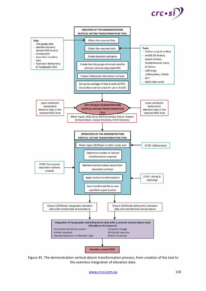
(refer to Section 8.2 & Figure 45) are resolved, it will be a relatively straight‐forward task to integrate
the data into a single elevation model.
1.2 PreviousWork
Previous vertical datum research in Australia has been conducted in Queensland and Western
Australia. In Queensland, the AUSHYDROID model relating the height of Chart Datum (CD) (LAT in
Australia ‐ refer to Section 3.2) to the World Geodetic System 1984 (WGS84) ellipsoid was developed
in 2004 (Martin and Broadbent, 2004; Todd et al, 2004). AUSHYDROID is the hydrographic equivalent
of AUSGeoid (discussed in Section 4.5). The model has been developed using the values of LAT and
the WGS84 ellipsoid at tidal stations, and extrapolating offshore, using the tidal zoning process,
explained as follows. In order to represent the curved CD/LAT surface, it is divided into a number of
zones (polygons). These polygons are called tidal zones and are small enough for the curved surface
within each zone to be regarded as planar. This approximation simplifies the estimation of the
CD/LAT elevation and thus the AUSHYDROID value at any point. The elevation of tidal datums other
than CD/LAT could also be interpolated in this way.
In some cases, tidal zoning can result in steps where discrete zones or tidal planes meet (CO‐OPS,
2007). AUSHYDROID was created using a triangulated irregular network (TIN) to avoid this problem.
However, statistical modelling such as used for AUSHYDROID is not as sophisticated a method for
modelling tidal datums as a hydrodynamic model (refer to Section 12.2). Hydrodynamic models are
very costly to build and there are few currently available. Where they are unavailable/unfeasible for
this project, statistical models such as AUSHYDROID will be required. At this stage, AUSHYDROID has
only been developed for the Queensland coast and for LAT to WGS84 conversions. A nationwide
implementation could provide a convenient means of datum transformation where hydrodynamic
models are absent and if the necessary tide gauge data could be acquired.
In February 2009 the Cooperative Research Centre for Spatial Information (CRCSI), with support
from Landgate and the Western Australian (WA) Department of Planning and Infrastructure,
conducted a pilot project to develop a general approach to vertical datum transformation across the
littoral zone (Seager, 2011a and 2011b). The project was based on a WA case study. The intention
www.crcsi.com.au 14
was to obtain topographic and bathymetric LiDAR data relative to the ellipsoid and to investigate
strategies for creating a seamless ellipsoidal height‐based DEM. Following this, methods for
transformation to other relevant reference frames such as AHD and tidal datums were to be
considered. However, at the time the researchers were unable to obtain reliable and accurate
ellipsoidal elevation data from the data providers.
The research concluded that systematic errors in the topographic data indicated a potential problem
with the methodology used to produce the ellipsoidal heights. However, these issues were resolved
whilst working with the data provider. The bathymetric LiDAR data was collected with the Fugro
LADS Mk II system. Although the bathymetric AHD data was found to be acceptable, systematic
errors were discovered in the ellipsoid height data. These errors manifested along the flight lines as
both “waves” and steps between adjacent flight lines and raised concerns over the data collection
and/or processing methodology. The research concluded that the supplied bathymetric data was not
suitable for deriving an offshore vertical datum transformation procedure.
This project continued the previous WA CRCSI research by following the aims and objectives set out
in Section 1.3. Further analysis has been performed on topographic and bathymetric LiDAR data in
new study areas. Bathymetric data from the new Fugro LADS Mk 3 system was tested and a
discussion on the outcomes of this analysis can be found in Section 6.
1.3 Aims&Objectives
The fundamental aim of this project was to facilitate the creation of seamless elevation datasets
across the Australian littoral zone by developing a method which enabled the transformation of
ellipsoid height/depth related data to other vertical datums of user interest (and vice versa). Given
this aim, and in the context of previous work, this led to the two primary objectives outlined below:
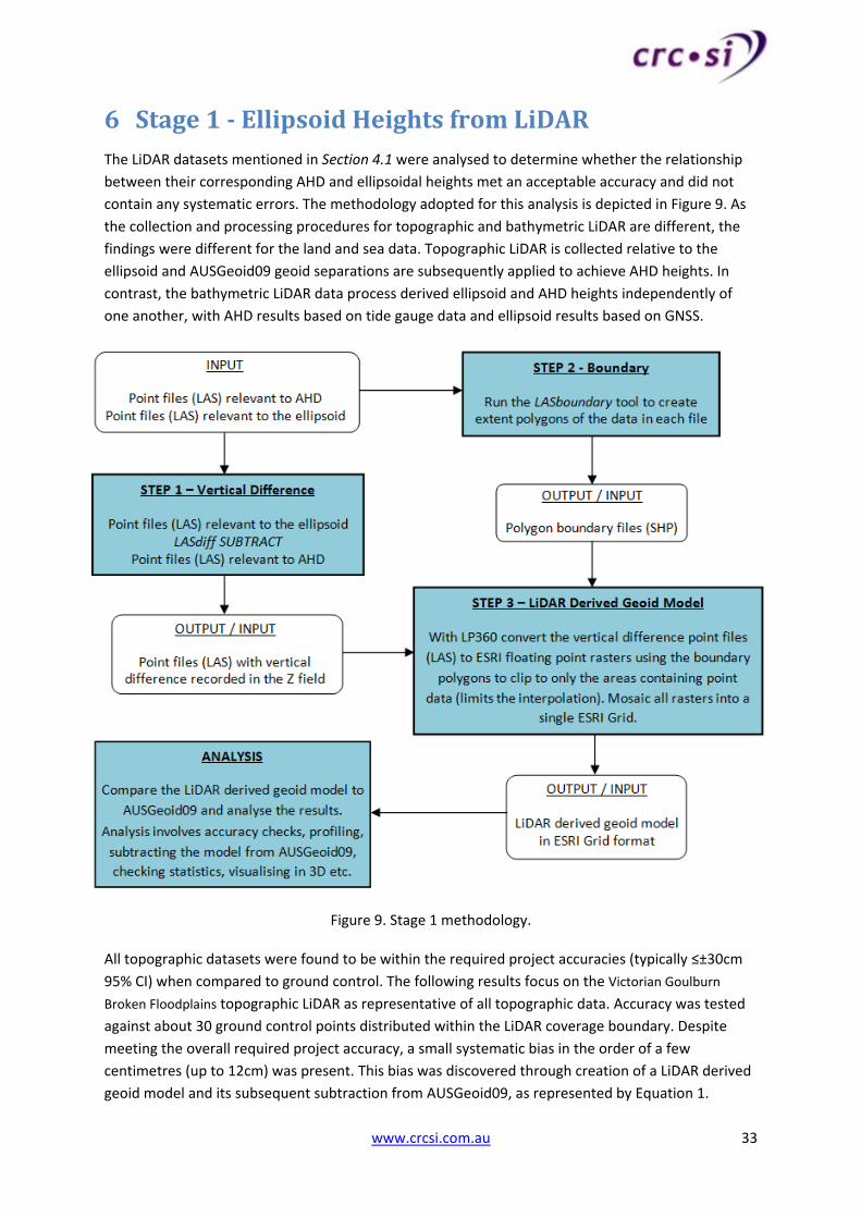
Stage 1 ‐ Ensure that ellipsoid‐based topographic and bathymetric LiDAR data can be
consistently and accurately produced in Australia.
Stage 2 ‐ Develop an ellipsoid‐based vertical datum transformation approach for land and near‐
shore elevation data, involving the development of a Demonstration Tool.
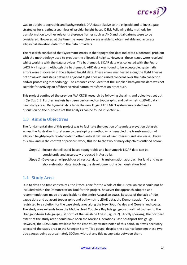
1.4 StudyArea
Due to data and time constraints, the littoral zone for the whole of the Australian coast could not be
included within the Demonstration Tool for this project, however the approach adopted and
recommendations made are applicable to the entire Australian coast. Because of the lack of tide
gauge data and adjacent topographic and bathymetric LiDAR data, the Demonstration Tool was
restricted to a solution for the case study area along the New South Wales and Queensland coasts.
The study area extends from the Middle Head Cobblers Bay tide gauge just north of Sydney, to the
Urangan Storm Tide gauge just north of the Sunshine Coast (Figure 2). Strictly speaking, the northern
extent of the study area should have been the Marine Operations Base Southport tide gauge.
However, the LiDAR data available for the case study existed north of this point, so it was necessary
to extend the study area to the Urangan Storm Tide gauge, despite the distance between these two
tide gauges being approximately 300km, without any tide gauge data between them.
www.crcsi.com.au 15
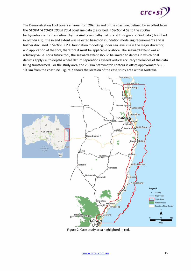
The Demonstration Tool covers an area from 20km inland of the coastline, defined by an offset from
the GEODATA COAST 1000K 2004 coastline data (described in Section 4.5), to the 2000m
bathymetric contour as defined by the Australian Bathymetric and Topographic Grid data (described
in Section 4.5). The inland extent was selected based on inundation modelling requirements and is
further discussed in Section 7.2.4. Inundation modelling under sea level rise is the major driver for,
and application of the tool, therefore it must be applicable onshore. The seaward extent was an
arbitrary value. For a future tool, the seaward extent should be limited to depths in which tidal
datums apply i.e. to depths where datum separations exceed vertical accuracy tolerances of the data
being transformed. For the study area, the 2000m bathymetric contour is offset approximately 30 ‐
100km from the coastline. Figure 2 shows the location of the case study area within Australia.
Figure 2. Case study area highlighted in red.
www.crcsi.com.au 16
2 BackgroundConcepts
2.1 AustralianTideGauges
Tide gauges provide an important record of coastal sea level. Tide gauge installations are usually
placed on piers and, as depicted in Figure 3 and Figure 4, consist of elements such as (PCTMSL,
2011);
A data recorder (short term recording device)
At least one water level sensor (there are a number of different types)
A method of communicating readings to users
A method of independently checking the height and time (e.g. a tide staff and clock)
A station height datum which water level heights are measured relative to
A tide gauge benchmark of known elevation relative to the station height datum as well as a
number of recovery benchmarks
Ideally devices for measuring wind speed, air and water temperature, and atmospheric
pressure so these environmental influences on the water level can be eliminated
More recently a permanent GNSS receiver to determine ellipsoidal height
The station height datum is an arbitrary value unique to each station, usually defined by the zero of
the first tide staff installed. It is established at an elevation below which the water is never expected
to fall. The station height datum is referenced to the tide gauge benchmark and is held constant.
Water level sensors continuously record the height of the water level with respect to the station
height datum allowing derivation of MSL and other tidal datums as required. To calculate MSL,
known as the ‘still water’ level, continuous measurements are averaged for a sufficient time period
to allow high frequency motions (e.g. wind waves) and periodic changes (e.g. tides) to be eliminated
(PSMSL, 2012). It is important to note that tidal datum heights vary spatially and temporally (refer to
Section 12.2).
Figure 3. Example of a common tide gauge measurement
system (CU, 2011).
Figure 4. SEA‐Level Fine Resolution Acoustic Measuring Equipment (SEAFRAME)1, Hillarys, WA (PCTMSL, 2011).
1 The NTC maintains 14 standard SEAFRAME stations (plus port operators own two supplementary stations) which
measure sea level very accurately. This SEAFRAME network is of a world leading standard.
www.crcsi.com.au 17
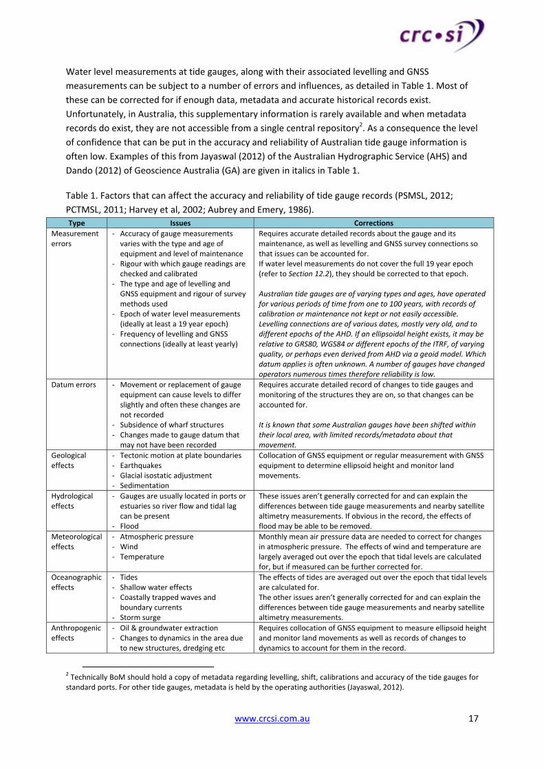
Water level measurements at tide gauges, along with their associated levelling and GNSS
measurements can be subject to a number of errors and influences, as detailed in Table 1. Most of
these can be corrected for if enough data, metadata and accurate historical records exist.
Unfortunately, in Australia, this supplementary information is rarely available and when metadata
records do exist, they are not accessible from a single central repository2. As a consequence the level
of confidence that can be put in the accuracy and reliability of Australian tide gauge information is
often low. Examples of this from Jayaswal (2012) of the Australian Hydrographic Service (AHS) and
Dando (2012) of Geoscience Australia (GA) are given in italics in Table 1.
Table 1. Factors that can affect the accuracy and reliability of tide gauge records (PSMSL, 2012;
PCTMSL, 2011; Harvey et al, 2002; Aubrey and Emery, 1986).
Type Issues Corrections
Measurement errors
‐ Accuracy of gauge measurements varies with the type and age of equipment and level of maintenance
‐ Rigour with which gauge readings are checked and calibrated
‐ The type and age of levelling and GNSS equipment and rigour of survey methods used
‐ Epoch of water level measurements (ideally at least a 19 year epoch)
‐ Frequency of levelling and GNSS connections (ideally at least yearly)
Requires accurate detailed records about the gauge and its maintenance, as well as levelling and GNSS survey connections so that issues can be accounted for. If water level measurements do not cover the full 19 year epoch (refer to Section 12.2), they should be corrected to that epoch. Australian tide gauges are of varying types and ages, have operated for various periods of time from one to 100 years, with records of calibration or maintenance not kept or not easily accessible. Levelling connections are of various dates, mostly very old, and to different epochs of the AHD. If an ellipsoidal height exists, it may be relative to GRS80, WGS84 or different epochs of the ITRF, of varying quality, or perhaps even derived from AHD via a geoid model. Which datum applies is often unknown. A number of gauges have changed operators numerous times therefore reliability is low.
Datum errors ‐ Movement or replacement of gauge equipment can cause levels to differ slightly and often these changes are not recorded
‐ Subsidence of wharf structures ‐ Changes made to gauge datum that may not have been recorded
Requires accurate detailed record of changes to tide gauges and monitoring of the structures they are on, so that changes can be accounted for. It is known that some Australian gauges have been shifted within their local area, with limited records/metadata about that movement.
Collocation of GNSS equipment or regular measurement with GNSS equipment to determine ellipsoid height and monitor land movements.
Hydrological effects
‐ Gauges are usually located in ports or estuaries so river flow and tidal lag can be present
‐ Flood
These issues aren’t generally corrected for and can explain the differences between tide gauge measurements and nearby satellite altimetry measurements. If obvious in the record, the effects of flood may be able to be removed.
Meteorological effects
‐ Atmospheric pressure ‐ Wind ‐ Temperature
Monthly mean air pressure data are needed to correct for changes in atmospheric pressure. The effects of wind and temperature are largely averaged out over the epoch that tidal levels are calculated for, but if measured can be further corrected for.
Oceanographic effects
‐ Tides ‐ Shallow water effects ‐ Coastally trapped waves and boundary currents
‐ Storm surge
The effects of tides are averaged out over the epoch that tidal levels are calculated for. The other issues aren’t generally corrected for and can explain the differences between tide gauge measurements and nearby satellite altimetry measurements.
Anthropogenic effects
‐ Oil & groundwater extraction ‐ Changes to dynamics in the area due to new structures, dredging etc
Requires collocation of GNSS equipment to measure ellipsoid height and monitor land movements as well as records of changes to dynamics to account for them in the record.
2 Technically BoM should hold a copy of metadata regarding levelling, shift, calibrations and accuracy of the tide gauges for standard ports. For other tide gauges, metadata is held by the operating authorities (Jayaswal, 2012).
www.crcsi.com.au 18
A significant issue affecting access to Australian tide gauge data is the lack of a central repository.
Data is currently held by the operators responsible for each gauge. A wide variety of institutions
operate the gauges including the National Tidal Centre (NTC), the AHS, the Australian Maritime
Safety Authority (AMSA), as well as many port authorities and state agencies. This makes collating
the data and calculating ellipsoidal MSL heights for Australian tide gauges a significant challenge in
its own right. The NTC is the primary source of tide tables, tidal streams and tidal constituents for
Australia and manage the national data archive for sea levels and tides. However, they only hold
data for major ports and do not currently act as a national repository for all Australian tide gauge
data. It is unclear what percentage of tide gauge data the NTC hold but using the Queensland coast
as an example, approximately 700 gauges exist while the NTC hold data just for the 34 major ports.
In comparison, the US has the Center for Operational Oceanographic Products and Services (CO‐OPS)
database, a publicly accessible website which makes available all coastal oceanographic products
and services. In the UK case, tide gauge data is accessible through the United Kingdom Hydrographic
Office (UKHO) which supplies onshore tide gauge data via the Admiralty Tide Tables (ATT) and also
holds data from offshore gauges (Turner et al, 2010). The tide gauge infrastructure and management
systems in Australia are not sufficient for a project such as this when compared to those in the US
and UK.
It should be noted that the AHS and the Intergovernmental Committee on Surveying and Mapping
(ICSM) Permanent Committee on Tides and Mean Sea Level (PCTMSL) have a joint project to collate
the ellipsoidal heights, levelling connections and tidal heights of continuously operated coastal tide
gauges which include major and some secondary ports. Uncertainties will be calculated for existing
data, and tide gauges with missing ellipsoidal heights, levelling connections or tidal heights will be
identified. However, there are 1000s of additional secondary tide gauges that are not incorporated
in this project. The project has been running for at least 5 years and remains ongoing with
completion expected by the end of 2012 (Jayaswal, 2012).
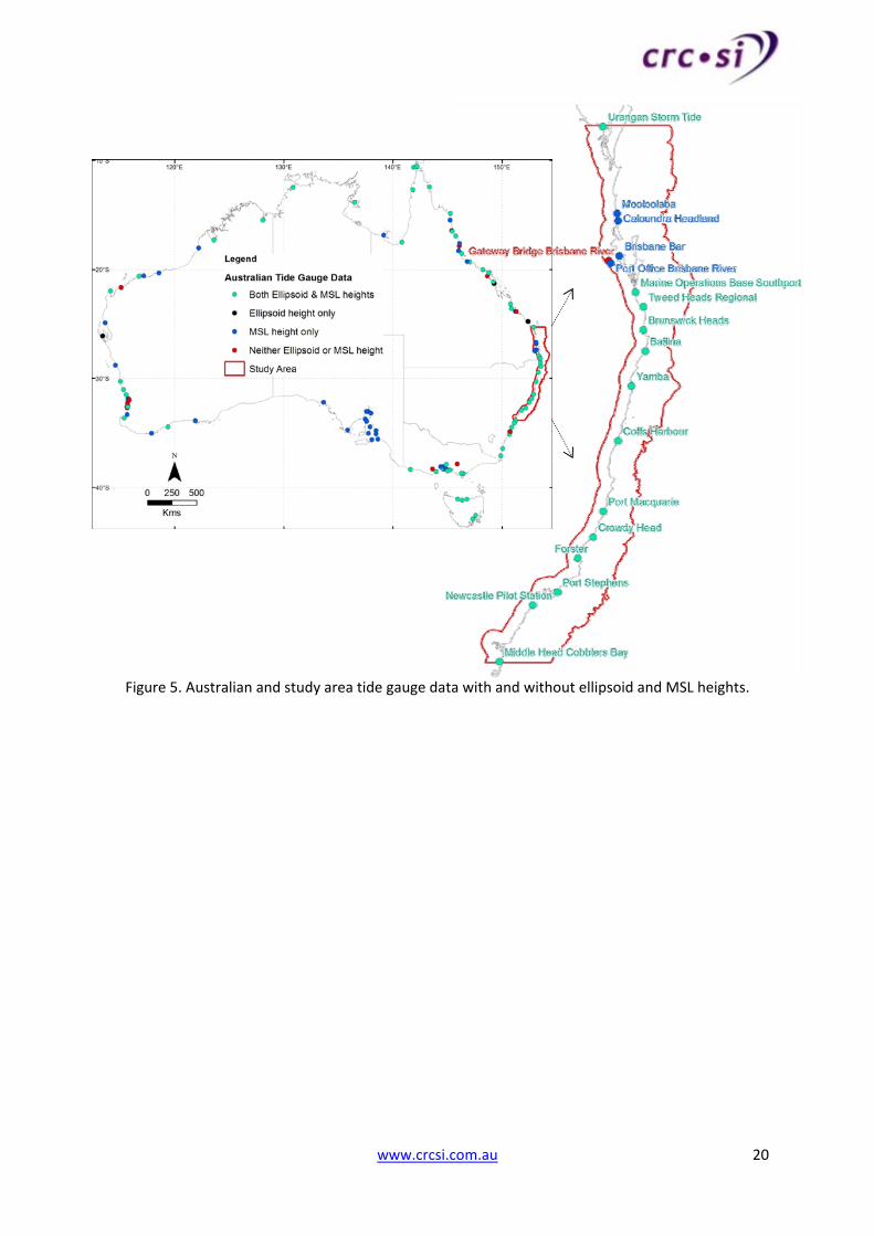
The AHS supplied the collated tide gauge data for the purposes of this project. This included 131
continuously operating coastal tide gauges around Australia including on islands, within rivers, and
Antarctic gauges. Of these, 111 have MSL values and 71 of these also have ellipsoid heights. Of the
71 gauges with the required data, after those in Antarctica and on distant islands are excluded, 67
remain (the quality of which is unknown) sparsely distributed along the nearly 36,000km of
Australian mainland coastline (60,000km including islands) (Figure 5). This is in contrast to the 1,987
gauges available for the about 8,200km of contiguous US coast for VDatum, and the 880 gauges to
represent around 18,000km of UK coastline (31,000km including major islands) for VORF. There
were 13 tide gauges with the required data available in the study area spread over a distance of
greater than 1,000km. These approximate coastline lengths illustrate the dramatic differences in the
density of tide gauges per kilometre of coastline.
Of the 67 Australian gauges, there are none in South Australia and in other areas there can be 100s
to 1000s of kilometres between gauges. The values of and relationships between tidal datums are
only known at the point locations of tide gauges where they are measured. At all locations other
than tide gauges, tidal datums must be estimated via modelling (refer to Sections 12.1 & 12.2).
Therefore a greater density of gauges leads to greater accuracy in modelling tidal datum surfaces.
This is especially true in areas of complex coastline such as rivers and bays. When transferring a tidal
www.crcsi.com.au 19
datum along the coast, the AHS recommends a maximum distance of 16km between gauges where
tidal conditions vary gradually, and 1.6km where conditions vary rapidly. The currently available
Australian gauges are too sparse to accurately model tidal datums around Australia. This assumption
is tested in (Section 7.2.1).
A fundamental requirement of this project is the derivation of ellipsoid MSL heights at tide gauges.
As mentioned, the AHS ICSM PCTMSL project provided this project with the data for continuously
operating coastal tide gauges around Australia (further discussed in Section 4.3). The data comes
from 19 different sources. Tidal datum, ellipsoid and AHD heights were provided adjusted relative to
LAT at the current National Tidal Datum Epoch (NTDE) of 1992‐2011 (refer to Section 12.2).
However, in a lot of cases there was missing information. For the study area (Figure 1), ellipsoidal
MSL heights were required for tide gauges from north of Sydney (the Middle Head Cobblers Bay
gauge), to just north of the Sunshine Coast (Urangan Storm Tide gauge). Five of the 18 gauges in this
area were missing ellipsoid heights, one of which was also missing a MSL height (Figure 5). It was not
possible to acquire or derive this missing data during the project.
Australian tide gauges with both MSL and ellipsoid height values are sparse. The data and metadata
are of unknown/varying quality and are difficult to access because there is no central repository. As
a result of these constraints, an accurate and reliable transformation tool which provides full
coverage of the Australian coast could not be produced unless the density and metadata is improved
for the tide gauge network. This project has produced a Demonstration Tool for a Map Grid of
Australia (MGA) Zone 56 study area as proof of the concept and recommendations have been made
about the need for improved tide gauge records. The procedure required to build the vertical datum
transformation tool for other areas of the Australian coastline is described in Appendix J.
www.crcsi.com.au 20
Figure 5. Australian and study area tide gauge data with and without ellipsoid and MSL heights.
www.crcsi.com.au 21
2.2 OtherBackgroundConcepts
In order to understand the approach adopted for coastal vertical datum transformation, there are a
number of additional background concepts that need to be understood. A summary of these
concepts follows and further information is contained in Appendix A. The concepts include;
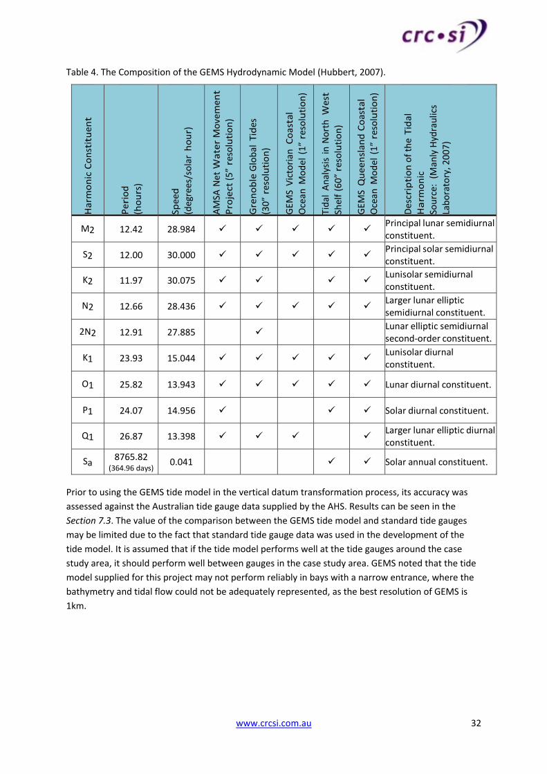
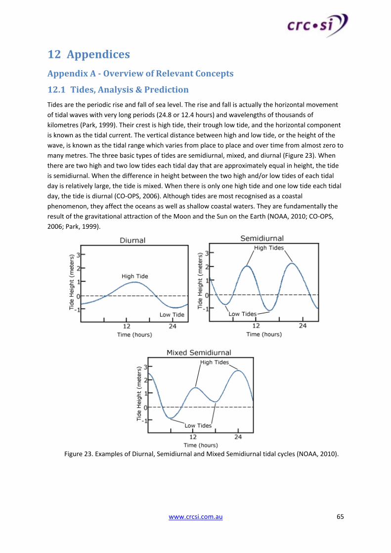
Tides, Analysis & Prediction
Tidal Datums & Models
Satellite Altimetry
Satellite Altimetry Derived Mean Sea Surface
Mean Dynamic Topography
Permanent Tide System
Spectral Content
The relevant marine reference surfaces are primarily tidal datums which can be determined at tide
gauges by averaging a particular phase of tide such as Mean High Water Springs (MHWS) or taking
the extreme values for LAT or Highest Astronomical Tide (HAT) (Section 12.1). However, at locations
other than tide gauges, modelling is required. Statistical modelling (interpolation/extrapolation) is
generally acceptable in the vicinity of primary tide gauges but elsewhere hydrodynamic models are a
more reliable way of estimating tide height. Hydrodynamic models are costly to build and there are
very few currently available. In Australia, Global Environmental Modelling Solutions (GEMS) is one of
only a very limited number of organisations that has developed a national tide model with a
resolution of better than 100km (Section 5.4). GEMS is the tide model used in the Demonstration
Tool and is discussed in Section 5.4. However GEMS could be replaced with a more accurate model
should one become available.
Satellite altimetry determines sea surface height relative to an ellipsoid. It provides centimetre
accurate measurements in the open oceans, but is less reliable near the coast. Satellite altimetry
should be used with caution within 22km of the Australian coastline and rejected entirely within
4km (Deng et al, 2010) (Section 12.3). A Mean Sea Surface (MSS) is a secondary gridded product of
satellite altimetry that represents the same physical variable as tide gauge MSL measurements. The
accuracy of a MSS is degraded from the original accuracy of altimetry sea surface height
measurements, to around three to ten centimetres (worse at the coast) (Andersen, 2012), due to
the additional data processing required to produce a MSS. Ellipsoidal MSL tide gauge measurements
can therefore be used to enhance a satellite altimetry derived MSS at the coast. The MSS used must
match the epoch and ellipsoid of the tide gauge data (Section 12.4).
A MSS comprises the geoid and Mean Dynamic Topography (MDT). MDT is the difference between
the geoid and the sea surface due to wind, atmospheric pressure, water temperature, salinity, and
currents. The determination of MDT around Australia would add to the understanding of the
relationships between vertical datums. It was not used to implement the transformation approach,
although is recommended for future development of a high accuracy tool. MDT was modelled as
part of the US and UK projects. If MDT is calculated with the direct method (MSS minus geoid), the
four issues to be considered are the ellipsoid, permanent tide system, spectral content (Section
12.7), and time period used (Section 12.5). It should be noted that development of a MDT should not
difference MSL and AUSGeoid09 heights. As AUSGeoid09 was warped to fit MSL, it largely contains
www.crcsi.com.au 22
MDT (Featherstone and Filmer, 2012) and would produce values typically smaller than true MDT. To
produce a MDT for Australia via the direct method, a geoid such as the Earth Gravitational Model
2008 (EGM08) or the gravimetric only component of AUSGeoid09 would be required.
The permanent earth tide is the tidal deformation of the Earth’s crust. The modelling of this
deformation has led to three definitions of the permanent earth tide; tide‐free, mean‐tide, and zero‐
tide systems. Corrections for the permanent tide system are intended to improve the precision of
geodetic measurement. When combining heights from various sources, they should all be relative to
the same permanent tide system to maximise precision. Equations and software are available to
convert the permanent tide system of relevant data. The Demonstration Tool adopts the tide‐free
system (Section 12.6).
3 ReviewofInternationalProjects
3.1 OverviewofProjects
A number of institutions have developed or are in the process of developing vertical datum
separation models. These have either been initiated for hydrographic purposes to enable the use of
GNSS for referencing depth measurements at sea, or, to enable the creation of seamless coastal
datasets. Canada surveyed many tide stations with GNSS and used hydrodynamic modelling and
satellite altimetry to produce ellipsoidal separation models in the early to mid 1990s (FIG, 2006;
Wells et al, 2004). France undertook the ‘BATHYELLI’ project in 2005 to develop ellipsoidal
separation models again using altimetry, tide gauge observations, and hydrodynamic modelling
(Pineau‐Guillou and Dorst, 2011). However, it is the more notable examples in the US and UK which
are discussed in more detail in this report.
The US, UK and Australian projects are summarised in Table 2. More extensive information on the
US VDatum and the UK VORF projects can be found in Appendix B. The following section discusses
the Australian situation with comparison made to the US and UK activities. The biggest impediment
to Australia, in adopting a methodology for vertical datum transformation, is the lack of quality tide
gauge data. Despite this, a broad approach has been developed similar to that of VORF, although
initiated for reasons akin to VDatum (refer to Appendix B).
www.crcsi.com.au 23
Table 2. Summary of Projects Reviewed. Refer to Appendix B Section 12.8 for further information.
US VDatum UK VORF Australia
Project Aim To support a seamless
bathymetric ‐ topographic digital elevation model (DEM).
Primarily navigational objectives i.e. to improve marine safety. Also for improved efficiency of hydrographic surveying etc.
To facilitate the creation of seamless DEMs spanning the land‐sea interface to study the
impacts of sea level rise.
Project Length 13 years 3 years 1 year to date
No. of Datums 36 24 6
Accuracy Evaluated in terms of the standard deviations.
10cm in coastal waters and 15cm in the open ocean (one standard
deviation). Unknown
Grid Resolution E.g. 0.05 degrees in latitude & 0.025 degrees in longitude.
Gridded at 0.008 degree intervals with patches of 0.003 degrees.
Demo Tool ‐ one minute resolution (~1‐2km).
Extent 1‐2km inland of the MHW to 25
nautical miles (46.3km) seaward.
UK and Irish continental shelves (not on land).
20km inland of the MHW coastline to the 2000m bathymetric contour.
Approach Minimum spanning tree Ellipsoid‐based Ellipsoid‐based
Modelling the difference between MSL and the geoid
TSS ‐ vertical separation between the orthometric height system NAVD88
geopotential surface and LMSL. Generated using tide gauge NAVD88 values & observed
tidal datums, plus hydrodynamic modelling.
SST – vertical separation between MSL and the OSGM05 geoid.
Generated by subtracting a tide gauge enhanced satellite
altimetry derived MSS from OSGM05.
MDT – N/A for Demo Tool. Fundamental approach ‐
vertical separation between MSL & the EGM2008 geoid.
Generated by subtracting a tide gauge enhanced satellite
altimetry derived MSS from EGM2008.
No. of Tide Gauges
1,987 880 67 (currently)
Modelling Tidal Datums
Existing hydrodynamic models and specially developed TCARI spatial interpolation technique.
Optimal combination of tide gauge tidal levels, hydrodynamic modelling, and satellite altimetry derived global ocean tide models.
GEMS hydrodynamic model. Other models can replace GEMS and/or specific
interpolation technique/s may need to be developed.
Permanent Tide System
Tide‐free Tide‐free Tide‐free
3.2 TheAustralianSituation
Australia has fewer applicable vertical datums than the UK or the US but a greater length of
coastline. The two most relevant vertical reference systems on land are the AHD and the GRS80
ellipsoid realised through the Geocentric Datum of Australia 1994 (GDA94)3. WGS84, other
realisations of ITRF, and the Australian National Spheroid (ANS) could also be considered but these
are excluded from this project for the reasons explained below.
The ANS was the ellipsoid behind Australia’s previous geodetic datum (AGD66/84). This datum is
now obsolete and therefore not considered further. There is a misconception that GDA94, WGS84
and ITRF are identical ‘for all practical purposes’. Although this remains a reasonable assumption for
low accuracy (~ >1m) applications, it was strictly only true in 1994 when GDA94 was realised. GDA94
is a static datum and since 1994, ITRF and WGS84 have gradually diverged from GDA94 due to the
tectonic motion of the Australian plate, and the ongoing refinement of the ITRF and WGS84 (GA,
2012). Although WGS84 and various realisations of ITRF are sometimes used in Australia, for the
Demonstration Tool, the ellipsoidal reference system of choice is limited to GRS80 realised as GDA94
as this is the official national datum.
3 GDA94 is the current geodetic datum in Australia. It based on ITRF92, realised at 1 January 1994.
www.crcsi.com.au 24
The horizontal coordinates of input data must also be in the applicable GDA94 MGA Zone. The
reasons for this are that GDA94 is the national datum of Australia and the majority of Australian
elevation data is referenced to MGA. If users possess elevation data relative to another reference
frame such as ITRF 2000, they will be required to pre‐transform to GDA94 using the parameters
provided on the GA website4. There is an intention to move Australia to a dynamic version of GDA in
2020 with the associated ellipsoidal height datum replacing AHD (Dando, 2012). ‘Working surfaces’
between the new ellipsoidal reference surface and AHD (equivalent to AUSGeoid09) as well as a
conventional geoid will be provided. If this intention is carried out, the transformation tool would
need to accommodate the change and incorporate the ‘working surfaces’.
In the marine environment, there are a greater number of vertical datums to consider. A list of tidal
datums as defined by the AHS tidal glossary is provided in Table 14 with those considered in this
project being LAT, MSL, MHWS, and HAT. Variations from the AHS definitions may occur in state
legislation however the AHS definitions have been adopted. In addition to the four tidal datums,
GRS80 ellipsoidal heights as mentioned above, and CD are applicable offshore. CD is the traditional
surface to refer depths to on a nautical chart. A CD is generally a tidal datum derived from a phase of
the tide, commonly LAT. CD on all current Australian nautical charts is LAT (Martin and Broadbent,
2004) predominantly for the current epoch 1992‐2011 however some of the charts first published on
LAT are still on the old epoch 1980‐1999. The first chart published on LAT in Australia was around
1994 based on a decision made by the AHS to meet technical Resolution A2.5 of the IHO and
standardise the CD in use (FIG, 2006). The CD in use before LAT was an approximation of Indian
Spring Low Water while port charts used an arbitrary port datum. Currently, the intention is to retain
CD as LAT 1992‐2011 until there is a LAT epoch that is different to the current epoch by +/‐ 0.1m.
This is not within the next 5‐10 years (Jayaswal, 2012). However, there is some debate around this as
when MSL is adjusted for sea level rise, high water predictions can be higher than HAT.
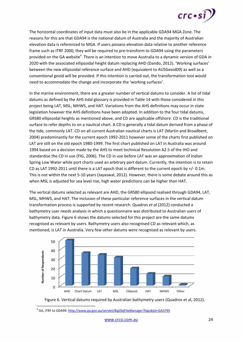
The vertical datums selected as relevant are AHD, the GRS80 ellipsoid realised through GDA94, LAT,
MSL, MHWS, and HAT. The inclusion of these particular reference surfaces in the vertical datum
transformation process is supported by recent research. Quadros et al (2012) conducted a
bathymetry user needs analysis in which a questionnaire was distributed to Australian users of
bathymetry data. Figure 6 shows the datums selected for this project are the same datums
recognised as relevant by users. Bathymetry users also recognised CD as relevant which, as
mentioned, is LAT in Australia. Very few other datums were recognised as relevant by users.
Figure 6. Vertical datums required by Australian bathymetry users (Quadros et al, 2012).
4 GA, ITRF to GDA94: http://www.ga.gov.au/servlet/BigObjFileManager?bigobjid=GA3795
0
10
20
30
40
50
AHD Chart Datum LAT MSL Ellipsoid HAT MHWS Other
Number of Respondents
www.crcsi.com.au 25
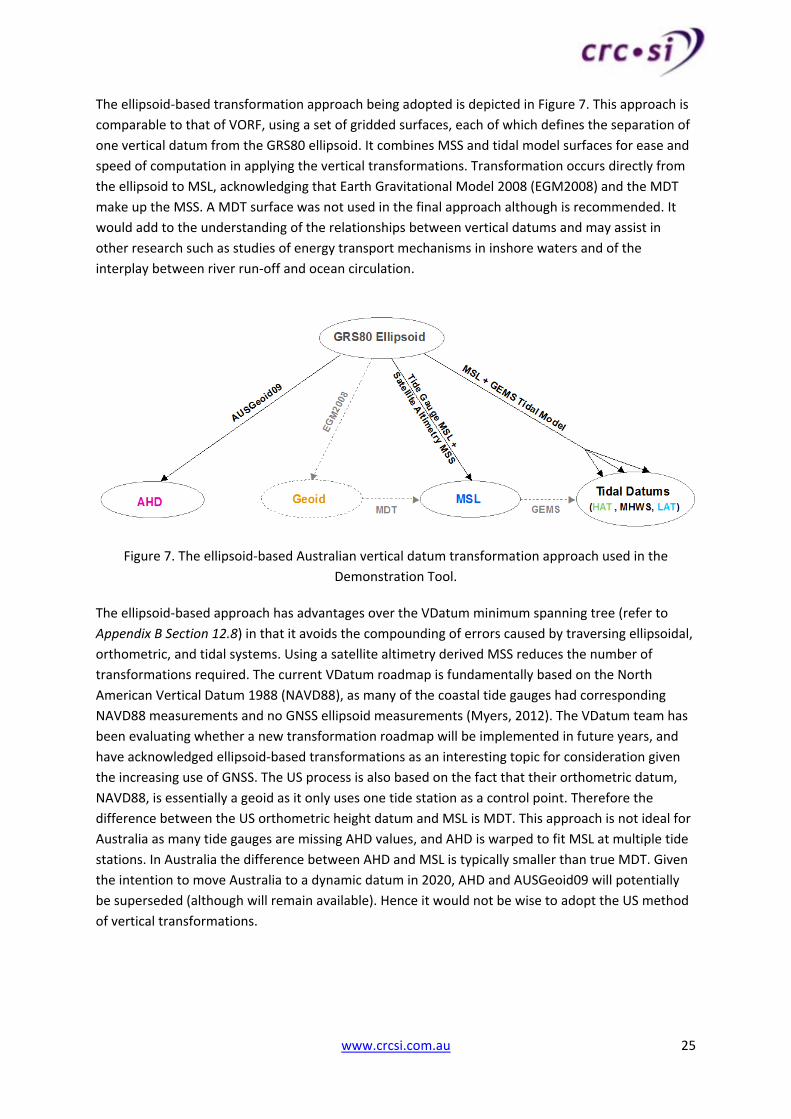
The ellipsoid‐based transformation approach being adopted is depicted in Figure 7. This approach is
comparable to that of VORF, using a set of gridded surfaces, each of which defines the separation of
one vertical datum from the GRS80 ellipsoid. It combines MSS and tidal model surfaces for ease and
speed of computation in applying the vertical transformations. Transformation occurs directly from
the ellipsoid to MSL, acknowledging that Earth Gravitational Model 2008 (EGM2008) and the MDT
make up the MSS. A MDT surface was not used in the final approach although is recommended. It
would add to the understanding of the relationships between vertical datums and may assist in
other research such as studies of energy transport mechanisms in inshore waters and of the
interplay between river run‐off and ocean circulation.
Figure 7. The ellipsoid‐based Australian vertical datum transformation approach used in the
Demonstration Tool.
The ellipsoid‐based approach has advantages over the VDatum minimum spanning tree (refer to
Appendix B Section 12.8) in that it avoids the compounding of errors caused by traversing ellipsoidal,
orthometric, and tidal systems. Using a satellite altimetry derived MSS reduces the number of
transformations required. The current VDatum roadmap is fundamentally based on the North
American Vertical Datum 1988 (NAVD88), as many of the coastal tide gauges had corresponding
NAVD88 measurements and no GNSS ellipsoid measurements (Myers, 2012). The VDatum team has
been evaluating whether a new transformation roadmap will be implemented in future years, and
have acknowledged ellipsoid‐based transformations as an interesting topic for consideration given
the increasing use of GNSS. The US process is also based on the fact that their orthometric datum,
NAVD88, is essentially a geoid as it only uses one tide station as a control point. Therefore the
difference between the US orthometric height datum and MSL is MDT. This approach is not ideal for
Australia as many tide gauges are missing AHD values, and AHD is warped to fit MSL at multiple tide
stations. In Australia the difference between AHD and MSL is typically smaller than true MDT. Given
the intention to move Australia to a dynamic datum in 2020, AHD and AUSGeoid09 will potentially
be superseded (although will remain available). Hence it would not be wise to adopt the US method
of vertical transformations.
www.crcsi.com.au 26
Australia is also unable to adopt one of the methods employed by the UK in which the datums of
some tide stations without a direct GNSS observation were connected to the European Terrestrial
Reference Frame 1989 (ETRF89) (a realisation of GRS80) by applying the OSGM02 geoid model. In
Australia’s case this would require the application of AUSGeoid09 to reliable AHD heights at stations
with missing ellipsoid heights. Thirty three of the supplied tide gauges are missing AHD heights and
those that are available are without metadata and considered generally unreliable as mentioned in
Section 2.1, so this method would not be acceptable. As the UK had metadata for their tide gauges,
they were able to acquire or directly commission GNSS observations where levelling heights (or
OSGM02) were unreliable (Iliffe et al, 2007).
Given the current lack of high quality tide gauge data in Australia, the transformation methodology
will be kept fairly broad for the Demonstration Tool which will act as a proof of concept rather than
an accurate transformation solution. There is little advantage to developing complex methodologies
based on current data which may prove invalid when denser, more accurate data is available.
Comprehensive methods for aligning the epoch of all tide gauge MSL values, such as the spatial‐
temporal correlation model used by VORF, are not developed. Currently, if observations span more
than one year they are generally assumed equivalent to the 19 year epoch and no corrections are
applied. This is because observations of greater than one year include seasonal variation in mean sea
level (harmonic constituent Sa) which has a period of about one year and is quite significant in
Australian waters. If observations span less than a year, a correction for seasonal variation may be
applied because sea level heights in winter can vary significantly from those in summer (Dando,
2012). This approach is accepted at this stage. Similarly, a simple method of interpolation between
tide gauge ellipsoidal MSL values along the coast is adopted, rather than developing a complex
method such as VDatum’s Tidal Constituent And Residual Interpolation (TCARI) or the specific
algorithms created by VORF for different types of coastal topography. Section 7.2 discusses the
interpolation methodology in more detail.
4 Data
4.1 LiDARData
The LiDAR data as described in Table 3 was obtained in the LiDAR LAS file format for this project. All
data supplied in both AHD and ellipsoid reference systems were analysed as part of Stage 1 of the
project. The demonstration of the software tool in the study area as part of Stage 2 of the project
used the Sunshine Coast datasets.
Table 3. LiDAR data obtained for the project.
Project Year Topo/Bathy Provider Reference System
Victorian Goulburn Broken
Floodplains 2010 Topographic Fugro Spatial AHD and Ellipsoid
Victorian Goulburn Broken
Floodplains 2011 Topographic Photomapping Services AHD and Ellipsoid
Sunshine Coast 2009 Topographic Schlencker Mapping Pty Ltd AHD
Sunshine Coast 2012 Bathymetric Fugro LADS AHD and Ellipsoid
www.crcsi.com.au 27
4.2 TheEarthGravitationalModel2008
EGM20085 can be accessed via the National Geospatial‐Intelligence Agency EGM Development Team
website. If a MDT were to be created for the transformation process, EGM2008 would be used to
transform input ellipsoid to geoid heights, as well as subtracted from the integrated MSS to
determine MDT values. AUSGeoid09 would not be used as it is warped to fit AHD which means the
difference between AUSGeoid09 and MSL is arbitrarily smaller than true MDT. EGM2008 is complete
to spherical harmonic degree and order 2159 and uses the tide‐free permanent tide system (NG‐IA,
2010). It is available in formats including an Environmental Systems Research Institute (ESRI) GRID
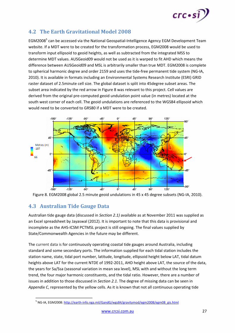
raster dataset of 2.5minute cell size. The global dataset is split into 45degree subset areas. The
subset area indicated by the red arrow in Figure 8 was relevant to this project. Cell values are
derived from the original pre‐computed geoid undulation point value (in metres) located at the
south west corner of each cell. The geoid undulations are referenced to the WGS84 ellipsoid which
would need to be converted to GRS80 if a MDT were to be created.
Figure 8. EGM2008 global 2.5 minute geoid undulations in 45 x 45 degree subsets (NG‐IA, 2010).
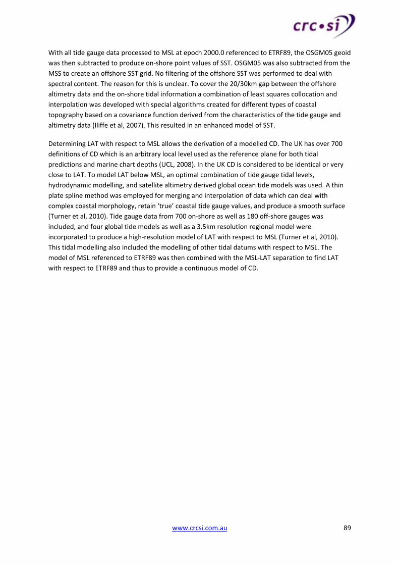
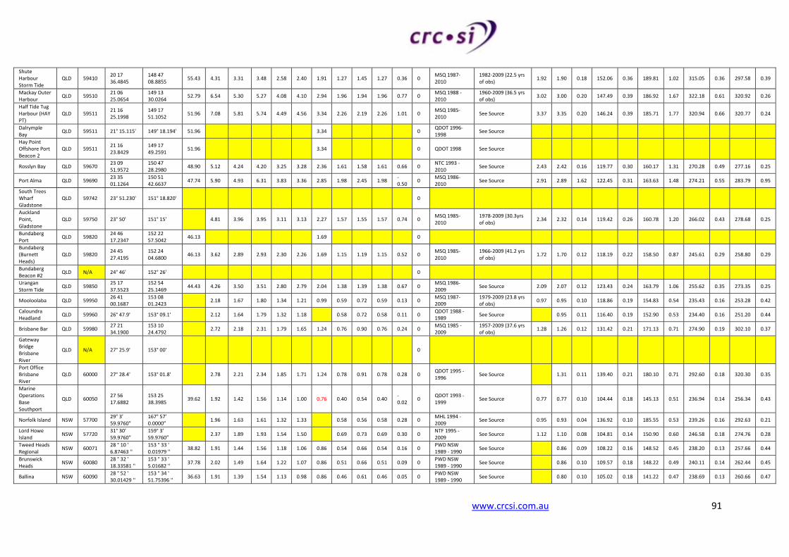
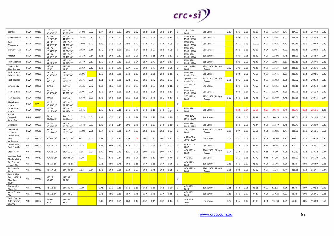
4.3 AustralianTideGaugeData
Australian tide gauge data (discussed in Section 2.1) available as at November 2011 was supplied as
an Excel spreadsheet by Jayaswal (2012). It is important to note that this data is provisional and
incomplete as the AHS‐ICSM PCTMSL project is still ongoing. The final values supplied by
State/Commonwealth Agencies in the future may be different.
The current data is for continuously operating coastal tide gauges around Australia, including
standard and some secondary ports. The information supplied for each tidal station includes the
station name, state, tidal port number, latitude, longitude, ellipsoid height below LAT, tidal datum
heights above LAT for the current NTDE of 1992‐2011, AHD height above LAT, the source of the data,
the years for Sa/Ssa (seasonal variation in mean sea level), MSL with and without the long term
trend, the four major harmonic constituents, and the tidal ratio. However, there are a number of
issues in addition to those discussed in Section 2.1. The degree of missing data can be seen in
Appendix C, represented by the yellow cells. As it is known that not all continuous operating tide
The DTU10 MSS is available in the mean‐tide system, relative to the Topex/Poseidon ellipsoid, and
the epoch 1993‐2009. For the purposes of the Demonstration Tool, this epoch was considered the
same as the NTDE used for the tide gauge data. The two epochs are similar and are centred over the
same period. The DTU10 MSS required conversion of its ellipsoid and tide system to the common
systems chosen. The GUT software (described in Section 5.3) was used to accurately convert the
ellipsoid and tide system.
The below GUT command line functions were used as a step by step workflow to achieve the two
conversions. Following the GUT conversions, the netCDF output file was imported into ArcGIS and
projected to GDA94 MGA Zone 56.
1. gut changeellipse_gf ‐InFile MSS_DTU_10_2M.nc ‐Ellipse GRS80 ‐OutFile MSSDTU10_GRS80.nc
2. gut changetide_gf ‐InFile MSSDTU10_GRS80.nc ‐OutFile MSSDTU10_GRS80_TF.nc ‐T tide‐free
The following sections discuss the four elements of the integrated MSS which are;
A tide gauge derived coastal ellipsoid‐based MSS extending 4km offshore
The satellite altimetry derived DTU10 MSS extending from 22km offshore to the open
ocean extent of the study area
Interpolation across the 4‐22km offshore satellite altimetry zone of caution between the
tide gauge MSS and the DTU10 MSS, rejecting low accuracy (error >0.03m) altimetry
data as defined by DTU10ERR
Extrapolation of the tide gauge MSS from the coastline to 20km inland
7.2.1 TideGaugeDerivedMeanSeaSurface
As mentioned in Section 12.3, Deng et al (2002) conducted a study of the contamination of satellite
altimetry data close to the coast of Australia. They recommended that data be used with caution for
distances less than about 22km from the coastline, and rejected altogether within 4km. Following
these recommendations, only the coastal tide gauge ellipsoidal MSL data was used within 4km of the
coastline. The UK also based their zone of exclusion of altimetry data on the work of Deng et al
(2002). VORF resolved to use only tide gauge data within 14km of the coast, purely satellite altimetry
outside a 30km buffer of the coast, and a combination of the two in between (Iliffe et al, 2007). For
this project, in order to ensure satellite altimetry data has no influence within its zone of exclusion,
the tide gauge data were first interpolated/extrapolated into a surface extending from the coastline
to 4km offshore. This gave the tide gauge data equal weighting to the altimetry in the latter
www.crcsi.com.au 40
interpolation across the 4‐22km zone of caution and resulted in a smoother integrated MSS than if
only the individual tide gauge points were used.
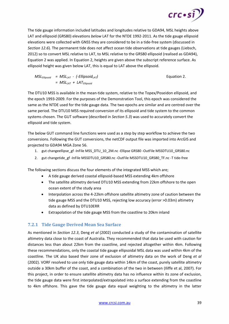
Before interpolating the tide gauge data, the behaviour of the sea surface along the east coast was
analysed. Values of EGM08 at each tide gauge location were subtracted from the tide gauge
ellipsoidal MSL to produce GPS‐geoid MDT point values. Figure 14 and Figure 15 show a linear
regression of the GPS‐geoid MDT as a function of latitude for the tide gauges along the east coast of
Australia. The regression line in Figure 14 has a slope of 49mm/degree of latitude and an R2 value of
0.2962. The removal of two outliers (perhaps due to errors in MSL or ellipsoid height) results in
Figure 15, with a slope of 25mm/degree and an R2 value of 0.5668. The limited sample of data
indicates some degree of correlation between MDT and latitude, and a North‐South slope in MDT,
which has been shown by others such as Featherstone and Filmer (2012). It should be noted that this
GPS‐geoid method of calculating MDT is adversely affected by the limitations of geoid models in the
coastal zone which can cause noise in the MDT values. Also, the tide gauge MSL values were not IB
corrected for the MDT calculation. As mean atmospheric pressure tends to decrease towards the
equator, it could account for some of the north‐south slope in the MDT. However Featherstone and
Filmer (2012) showed the IB influence to be ‐2.8mm/degree which is much smaller than the slope of
MDT.
Figure 14. GPS‐geoid MDT (metres) plotted against latitude (degrees) for all east coast tide
gauges. Study area gauges shown in black.
www.crcsi.com.au 41
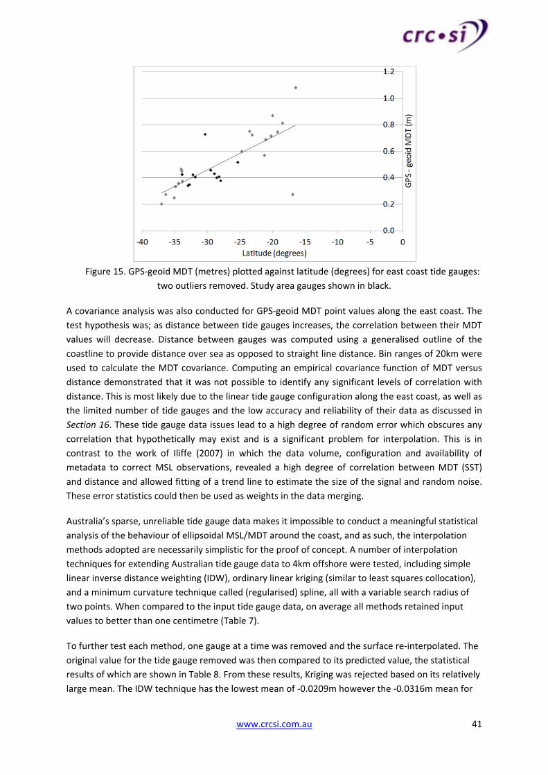
Figure 15. GPS‐geoid MDT (metres) plotted against latitude (degrees) for east coast tide gauges:
two outliers removed. Study area gauges shown in black.
A covariance analysis was also conducted for GPS‐geoid MDT point values along the east coast. The
test hypothesis was; as distance between tide gauges increases, the correlation between their MDT
values will decrease. Distance between gauges was computed using a generalised outline of the
coastline to provide distance over sea as opposed to straight line distance. Bin ranges of 20km were
used to calculate the MDT covariance. Computing an empirical covariance function of MDT versus
distance demonstrated that it was not possible to identify any significant levels of correlation with
distance. This is most likely due to the linear tide gauge configuration along the east coast, as well as
the limited number of tide gauges and the low accuracy and reliability of their data as discussed in
Section 16. These tide gauge data issues lead to a high degree of random error which obscures any
correlation that hypothetically may exist and is a significant problem for interpolation. This is in
contrast to the work of Iliffe (2007) in which the data volume, configuration and availability of
metadata to correct MSL observations, revealed a high degree of correlation between MDT (SST)
and distance and allowed fitting of a trend line to estimate the size of the signal and random noise.
These error statistics could then be used as weights in the data merging.
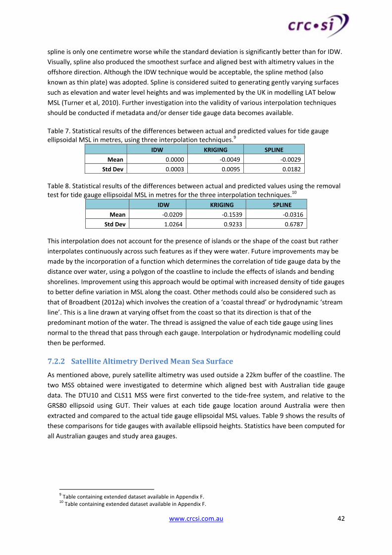
Australia’s sparse, unreliable tide gauge data makes it impossible to conduct a meaningful statistical
analysis of the behaviour of ellipsoidal MSL/MDT around the coast, and as such, the interpolation
methods adopted are necessarily simplistic for the proof of concept. A number of interpolation
techniques for extending Australian tide gauge data to 4km offshore were tested, including simple
linear inverse distance weighting (IDW), ordinary linear kriging (similar to least squares collocation),
and a minimum curvature technique called (regularised) spline, all with a variable search radius of
two points. When compared to the input tide gauge data, on average all methods retained input
values to better than one centimetre (Table 7).
To further test each method, one gauge at a time was removed and the surface re‐interpolated. The
original value for the tide gauge removed was then compared to its predicted value, the statistical
results of which are shown in Table 8. From these results, Kriging was rejected based on its relatively
large mean. The IDW technique has the lowest mean of ‐0.0209m however the ‐0.0316m mean for
www.crcsi.com.au 42
spline is only one centimetre worse while the standard deviation is significantly better than for IDW.
Visually, spline also produced the smoothest surface and aligned best with altimetry values in the
offshore direction. Although the IDW technique would be acceptable, the spline method (also
known as thin plate) was adopted. Spline is considered suited to generating gently varying surfaces
such as elevation and water level heights and was implemented by the UK in modelling LAT below
MSL (Turner et al, 2010). Further investigation into the validity of various interpolation techniques
should be conducted if metadata and/or denser tide gauge data becomes available.
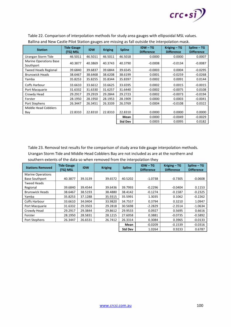
Table 7. Statistical results of the differences between actual and predicted values for tide gauge ellipsoidal MSL in metres, using three interpolation techniques.9
IDW KRIGING SPLINE
Mean 0.0000 ‐0.0049 ‐0.0029
Std Dev 0.0003 0.0095 0.0182
Table 8. Statistical results of the differences between actual and predicted values using the removal test for tide gauge ellipsoidal MSL in metres for the three interpolation techniques.10
IDW KRIGING SPLINE
Mean ‐0.0209 ‐0.1539 ‐0.0316
Std Dev 1.0264 0.9233 0.6787
This interpolation does not account for the presence of islands or the shape of the coast but rather
interpolates continuously across such features as if they were water. Future improvements may be
made by the incorporation of a function which determines the correlation of tide gauge data by the
distance over water, using a polygon of the coastline to include the effects of islands and bending
shorelines. Improvement using this approach would be optimal with increased density of tide gauges
to better define variation in MSL along the coast. Other methods could also be considered such as
that of Broadbent (2012a) which involves the creation of a ‘coastal thread’ or hydrodynamic ‘stream
line’. This is a line drawn at varying offset from the coast so that its direction is that of the
predominant motion of the water. The thread is assigned the value of each tide gauge using lines
normal to the thread that pass through each gauge. Interpolation or hydrodynamic modelling could
then be performed.
7.2.2 SatelliteAltimetryDerivedMeanSeaSurface
As mentioned above, purely satellite altimetry was used outside a 22km buffer of the coastline. The
two MSS obtained were investigated to determine which aligned best with Australian tide gauge
data. The DTU10 and CLS11 MSS were first converted to the tide‐free system, and relative to the
GRS80 ellipsoid using GUT. Their values at each tide gauge location around Australia were then
extracted and compared to the actual tide gauge ellipsoidal MSL values. Table 9 shows the results of
these comparisons for tide gauges with available ellipsoid heights. Statistics have been computed for
all Australian gauges and study area gauges.
9 Table containing extended dataset available in Appendix F. 10 Table containing extended dataset available in Appendix F.
www.crcsi.com.au 43
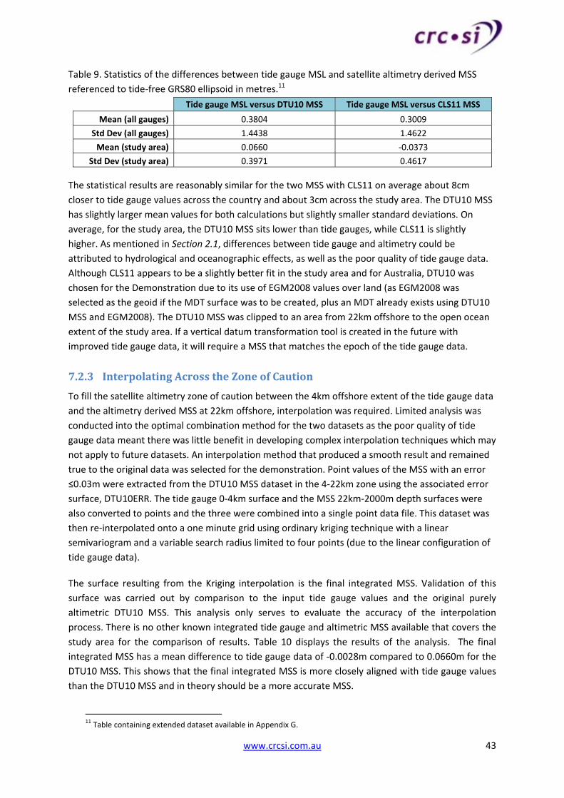
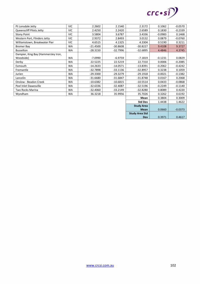
Table 9. Statistics of the differences between tide gauge MSL and satellite altimetry derived MSS
referenced to tide‐free GRS80 ellipsoid in metres.11
Tide gauge MSL versus DTU10 MSS Tide gauge MSL versus CLS11 MSS
Mean (all gauges) 0.3804 0.3009
Std Dev (all gauges) 1.4438 1.4622
Mean (study area) 0.0660 ‐0.0373
Std Dev (study area) 0.3971 0.4617
The statistical results are reasonably similar for the two MSS with CLS11 on average about 8cm
closer to tide gauge values across the country and about 3cm across the study area. The DTU10 MSS
has slightly larger mean values for both calculations but slightly smaller standard deviations. On
average, for the study area, the DTU10 MSS sits lower than tide gauges, while CLS11 is slightly
higher. As mentioned in Section 2.1, differences between tide gauge and altimetry could be
attributed to hydrological and oceanographic effects, as well as the poor quality of tide gauge data.
Although CLS11 appears to be a slightly better fit in the study area and for Australia, DTU10 was
chosen for the Demonstration due to its use of EGM2008 values over land (as EGM2008 was
selected as the geoid if the MDT surface was to be created, plus an MDT already exists using DTU10
MSS and EGM2008). The DTU10 MSS was clipped to an area from 22km offshore to the open ocean
extent of the study area. If a vertical datum transformation tool is created in the future with
improved tide gauge data, it will require a MSS that matches the epoch of the tide gauge data.
7.2.3 InterpolatingAcrosstheZoneofCaution
To fill the satellite altimetry zone of caution between the 4km offshore extent of the tide gauge data
and the altimetry derived MSS at 22km offshore, interpolation was required. Limited analysis was
conducted into the optimal combination method for the two datasets as the poor quality of tide
gauge data meant there was little benefit in developing complex interpolation techniques which may
not apply to future datasets. An interpolation method that produced a smooth result and remained
true to the original data was selected for the demonstration. Point values of the MSS with an error
≤0.03m were extracted from the DTU10 MSS dataset in the 4‐22km zone using the associated error
surface, DTU10ERR. The tide gauge 0‐4km surface and the MSS 22km‐2000m depth surfaces were
also converted to points and the three were combined into a single point data file. This dataset was
then re‐interpolated onto a one minute grid using ordinary kriging technique with a linear
semivariogram and a variable search radius limited to four points (due to the linear configuration of
tide gauge data).
The surface resulting from the Kriging interpolation is the final integrated MSS. Validation of this
surface was carried out by comparison to the input tide gauge values and the original purely
altimetric DTU10 MSS. This analysis only serves to evaluate the accuracy of the interpolation
process. There is no other known integrated tide gauge and altimetric MSS available that covers the
study area for the comparison of results. Table 10 displays the results of the analysis. The final
integrated MSS has a mean difference to tide gauge data of ‐0.0028m compared to 0.0660m for the
DTU10 MSS. This shows that the final integrated MSS is more closely aligned with tide gauge values
than the DTU10 MSS and in theory should be a more accurate MSS.
11 Table containing extended dataset available in Appendix G.
www.crcsi.com.au 44
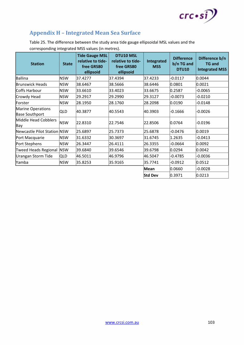
Table 10. Analysis of the difference between tide gauge ellipsoidal MSL and corresponding integrated MSS values (in metres).12
Tidal gauge MSL subtract MSS
DTU10 MSS Final Integrated MSS
Mean 0.0660 ‐0.0028
Standard Deviation 0.3971 0.0213
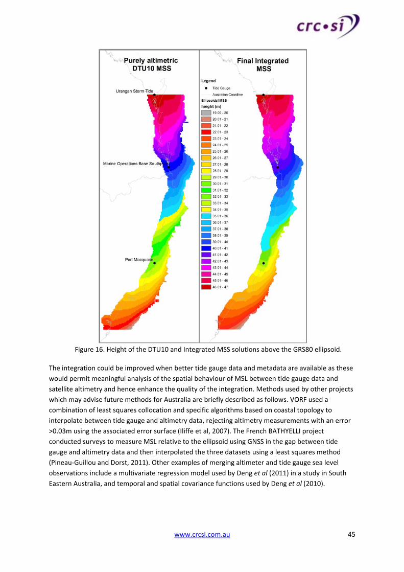
The final form of the MSS within the study area is shown in Figure 16. The surfaces are similar
although the finer resolution of the integrated MSS is apparent, along with a different height pattern
as a result of the assimilated tide gauge data. There are two notable differences. Firstly, between the
Marine Operations Base Southport gauge just south of South Stradbroke Island and the Urangan
Storm Tide gauge at the northern extent of the study area, there is a different spatial pattern of
heights when compared to the DTU10 MSS. As there are no tide gauges between these locations (an
approximately 300km linear distance), the form of the integrated MSS in this area cannot be relied
upon. Additional tide gauge data is required to improve the accuracy of the integrated MSS in this
region.
The second major disparity is in the region centred on the Port Macquarie gauge where higher
values in the integrated MSS dip further south than in the DTU10 MSS. When considering the study
area gauges, the difference between ellipsoidal MSL and the DTU10 MSS for Port Macquarie is
significantly higher than for any other gauge, with a value of 1.2635m compared to the mean of
0.0660m (Appendix G). This difference is most likely because the Port Macquarie gauge is protected
from some of the general ocean effects due to its position just south west of Lady Nelson Wharf and
may also be highly influenced by the Hastings River. As mentioned in Table 1, hydrological and
oceanographic effects such as these can explain differences between tide gauge and satellite
altimetry data. As these issues can’t generally be corrected for, gauges experiencing these kinds of
effects could have a weighting applied to limit their influence on the interpolation. Alternatively,
such gauges could be removed from the interpolation if temporary gauges could be established in
nearby open coast locations, or fixed to the sea floor offshore outside the range of shallow water
effects. As the Demonstration Tool is simply a proof of concept, the Port Macquarie gauge was not
removed from the integrated surface. Ultimately, increased density of tide gauge data in this region
would prevent the influences of this tide gauge due to its position, from being propagated beyond
the area it directly affects. This would improve the accuracy of modelled MSL.
12 Table containing extended dataset available in Appendix H.
www.crcsi.com.au 45
Figure 16. Height of the DTU10 and Integrated MSS solutions above the GRS80 ellipsoid.
The integration could be improved when better tide gauge data and metadata are available as these
would permit meaningful analysis of the spatial behaviour of MSL between tide gauge data and
satellite altimetry and hence enhance the quality of the integration. Methods used by other projects
which may advise future methods for Australia are briefly described as follows. VORF used a
combination of least squares collocation and specific algorithms based on coastal topology to
interpolate between tide gauge and altimetry data, rejecting altimetry measurements with an error
>0.03m using the associated error surface (Iliffe et al, 2007). The French BATHYELLI project
conducted surveys to measure MSL relative to the ellipsoid using GNSS in the gap between tide
gauge and altimetry data and then interpolated the three datasets using a least squares method
(Pineau‐Guillou and Dorst, 2011). Other examples of merging altimeter and tide gauge sea level
observations include a multivariate regression model used by Deng et al (2011) in a study in South
Eastern Australia, and temporal and spatial covariance functions used by Deng et al (2010).
www.crcsi.com.au 46
7.2.4 OnshoreExtrapolation
As the vertical datum transformation tool is intended to facilitate the integration of topographic and
bathymetric data, the vertical transformations need to extend onshore. Although tidal datums have
no physical meaning onshore, they do become relevant for example if the land is inundated by
floods or tides in the case of storm surge or seal level rise, or for the processing of LiDAR data to
determine shorelines. The VORF project did not extend onshore, as navigational objectives drove
and funded the work. The US did extrapolate their tidal datums inland to a distance of 1‐2km, and
plan to enhance VDatum by extending these further inland (NOAA, 2011). For the Demonstration
Tool, MSL has been extrapolated to a distance of 20km inland to enable inundation modelling. The
generally accepted elevation extent for coastal inundation modelling in Australia is ten metres above
MSL. Although the 20km distance selected is conservative, it should encompass the majority of the
Australian coast within the ten metre elevation extent.
The extrapolation was achieved as part of the kriging process discussed in Section 7.2.3 by defining
the extent as a 20km inland offset from the coastline. As no sea level data exists between the coast
and this 20km offset, technically extrapolation occurred in this region. For the demonstration,
kriging was deemed an acceptable extrapolator, with other methods tested returning very similar
results. GEMS is capable of modelling over land (for the purpose of inundation), so the other tidal
datums were simply offset from MSL without the need for extrapolation.
There are a number of issues with extrapolating tidal datums inland. Spatial variations in tidal
datums near the shore can influence the method of approximating their extension inland. For
example, in Figure 17 the locations starred in red present potential problems because they are close
to two different bodies of water for which different heights may represent the same tidal datums.
This issue could be addressed by using breaklines and/or an algorithm for distance over sea.
However if tidal datums are spatially uniform, extrapolation can usually be done by assuming an
average constant datum difference or by using an interpolation method. In Australia’s case (as
discussed in Section 7.2.1), the variability of tidal datums along the coast and between different
coastal regimes (e.g. river, bay, ocean, tidal flats, etc.) is smooth enough to allow interpolation to be
used as an extrapolator for the Demonstration Tool. Closer investigation of the validity of using
interpolation methods to extrapolate tidal datums inland for the Australian coast should occur in the
future when denser tide gauge data are available.
Figure 17. Locations starred in red that are potential problems for inland tidal datum extrapolation.
www.crcsi.com.au 47
7.3 EllipsoidtoTidalDatums
Transformations to the tidal datums LAT, MHWS, and HAT were achieved via the GEMS
hydrodynamic model discussed in Section 5.4. The GEMS model was tested against current tide
gauge data by running the tide gauge coordinates through GEMS. Before GEMS results could be
compared to tide gauge values of LAT, MHWS, and HAT, the tide gauge data had to be converted so
they were relative to MSL rather than LAT. Equations 3‐3.2 were used, where the subscript is the
reference surface that heights are relative to.
LATMSL = ‐ MSLLAT Equation 3.
MHWSMSL = MHWSLAT ‐ MSLLAT ...3.1
HATMSL = HATLAT ‐ MSLLAT ...3.2
Table 11 shows the results of these comparisons for tide gauges with available tidal datum heights.
Statistics were computed separately for all gauges and study area gauges. Three possible outliers can
be seen in Appendix H highlighted in pink, all of which are in Queensland, north of the study area. It
is known that GEMS has not been properly calibrated in northern Queensland but as this is outside
the study area, it has no impact on the Demonstration Tool. When compared to current tide gauge
data across Australia, GEMS performed best for LAT, with a mean of ‐13cm. On average GEMS
results put LAT and MHWS below tide gauge values and HAT above. Statistics for study area gauges
are similar to the statistics for all gauges for the datums HAT and LAT, while results for MHWS are
significantly better with a study area mean of ‐2cm. The reason for this is not clear although, it is
perhaps linked to GEMS not being calibrated in some places outside the study area which may affect
MHWS more than HAT and LAT as it is an average value as opposed to an extreme. GEMS generally
produces results within 10‐20cm of current tide gauge values. Although the GEMS tidal model may
be able to be improved and updated with more recent bathymetry in some areas, it performs
reasonably well when compared to current Australian tide gauge information and hence was utilised
in the demonstration vertical datum transformation tool.
Table 11. Differences between tide gauge tidal datums relative to MSL & GEMS results in metres. 13
Tidal gauge datum values subtract GEMS results
HAT LAT MHWS
Mean (all) 0.21 ‐0.13 ‐0.15
Standard Deviation (all) 0.46 0.46 0.39
Study Area Mean 0.22 ‐0.15 ‐0.02
Study Area Standard Deviation 0.32 0.22 0.21
To develop the ellipsoidal tidal datum separation surfaces, a point grid with one kilometre spacing
was generated for the study area. Ideally this point spacing should be closer to 100m to capture all
coastal variation in the tidal datums however to save time and processing, a larger value was
selected given the MSS grid has only been developed at one minute resolution (~1‐2km). The grid of
point ‘stations’ was run through GEMS to produce MSL to LAT, MHWS and HAT offsets for each
point. These offsets were interpolated into gridded surfaces using the spline minimum curvature
technique as used for the coastal MSL interpolation. Each tidal surface was then individually added
to the final integrated MSS to produce three gridded ellipsoidal tidal datum separation surfaces to
the centimetre level for use in the transformation tool. As GEMS is capable of producing output over
13 Table containing extended dataset available in Appendix I.
www.crcsi.com.au 48
land (for the purposes of inundation modelling), no extrapolation of the tidal surfaces was required.
By producing these separation surfaces, the GEMS model does not have to be integrated into the
Demonstration Tool which saves significant time in the transformation process, as GEMS executes
slowly.
The results for the HAT tidal datum are shown in Figure 18. The interpolated output from GEMS is on
the left, and interestingly, reveals a pattern of circles along the coast. These circles are centred on
tide gauges which suggests that, contrary to the information available, GEMS has a statistical model
component which matches to the tide gauges as opposed to purely being a physical model which
uses boundary conditions to replicate the tidal behaviour within the area of applicability. A pure
physical model would not take tide gauge data as direct input, but use it only for calibration. The
pattern produced by GEMS, aside from the circles, is strange and can only be attributed to the inner
workings of the model itself. The same pattern was found for the LAT and MHWS results and carries
through to the final separation surfaces. GEMS has been used for the Demonstration Tool but these
results provide further impetus to source an improved model/s for any future vertical datum
transformation tool.
Figure 18. Results for HAT. The left image is the interpolated GEMS HAT above MSL output, and the
right image is the final separation surface HAT relative to the GRS80 ellipsoid (in metres).
Pattern of tide gauge circles carry through to the final separation surfaces.
www.crcsi.com.au 49
7.4 TheDemonstrationTool
The Demonstration Tool was developed in the Python 2.5 programming language and runs as an
ArcToolbox geoprocessing script with an ArcInfo license of ArcGIS 10.0 or with the Spatial Analyst
and 3D Analyst extensions. A package of data and tools are required for the operation of the tool,
and must all be located within one folder and named exactly as described in inverted commas
below. A sample of this data for the project study area is supplied however the user can supply data
for other areas of Australia which can be produced following the steps in Appendix J. The folder
location of this data or Demonstration Tool Data Package (DTDP) is an input requirement for the tool
and must contain;
The ESRI GRID format vertical separation surfaces (sample data supplied was developed as
part of the project for the MGA Z56 study area discussed in Section 7)
o ellipsoid‐MSL – “integmss”
o ellipsoid‐LAT – “ell_lat”
o ellipsoid‐MHWS – “ell_mhws”
o ellipsoid‐HAT – “ell_hat”
o ellipsoid‐AHD – “ausgeoid09”
A polygon shapefile describing the extent of the transformation surfaces named
“StudyArea_bound.shp” (sample data supplied)
The LAStools; “lasboundary.exe”, “lasclip.exe” and “lasmerge.exe”. These are not supplied
with the sample DTDP as may require licensing as discussed in Section 5.1. They must be
obtained to use the tool.
Also supplied with the sample DTDP is an example input LAS file (“SunshineBathy2011‐C2‐
ELL_5137053_56_0001_0001.las”) and an ESRI GRID raster DEM file (“e513705201005”) with which
to test as input to the tool. Rasters of other formats can also be used as input. These files are both in
MGA Z56. The LAS file is relevant to the ellipsoid and the raster to AHD. The tool is provided “as‐is”
and is licensed under ‘Attribution‐ShareAlike 3.0 Australia (CC BY‐SA 3.0)’ meaning users are free to
copy, distribute, display, and perform the work, to make derivative works, and to make commercial
use of the work. However, if users alter, transform, or build upon this work, they may distribute the
resulting work only under a licence identical to this one and must give the original author credit.
If problems are experienced with the tool, some issues to be aware of are as follows. The use of
LAStools may mean there is a limit to the size of LAS files that can be processed (you may receive
warnings during processing). The spatial reference of rasters must be defined using the ESRI
convention for the MGA projection otherwise the tool will fail. It may be best to avoid spaces and
long path names for the tool and input files. When a raster file is input, the process may produce a
lock file that cannot be removed until the software is exited (an ESRI bug). If the tool claims it cannot
create an output, exit ArcMap, then re‐open it to re‐run the tool. This unfortunately means the tool
cannot be run in batch mode for raster files. It can however be run in batch mode for LAS files.
www.crcsi.com.au 50
Figure 19 outlines the transformation process applied by the tool. The majority of Australian
elevation data exist in MGA projected coordinates and the study area falls within MGA Zone 56.
Therefore the Demonstration Tool requires the horizontal coordinates of input data to be in GDA94
MGA Zone 56 unless the user is providing their own separation surfaces in another MGA Zone. In the
unlikely scenario that data are not in an MGA Zone, pre‐transformation to this system is required. A
tool that covers the entire Australian coast would ideally be capable of accepting either GDA94 or
MGA coordinates, to deal with projects that cross zones or to avoid horizontal transformation of
data which is in one zone before input.
Figure 19. Overview of the Demonstration Tool vertical datum transformation process
www.crcsi.com.au 51
Figure 20 shows the transformation tool’s interface. Six inputs are required to perform the
transformation. The user must provide either a LAS file or raster file in one of the first two input
boxes. When one of these files is selected, the other box is disabled. The tool then requires the user
to enter the MGA Zone of input data (56 if using the supplied DTDP), the vertical datum of the input
data (which must be one of the relevant six), as well as the desired output vertical datum (which also
must be one of the six). As these must be different, the vertical datum selected as input is excluded
from the output datum options. The user is also required to identify two directories. These include
where to save the transformed file, and the location of the DTDP. In this mode the tool only
transforms one LAS or GRID file at a time however it can be run in ‘Batch’ mode (for LAS files) as with
other geoprocessing tools to process multiple files. In this way the tool can be run once for a project
containing many tiles.
Figure 20. Demonstration Tool interface and example input.
The average processing times for the Demonstration Tool are shown in Table 12. The tool performs
efficiently for raster files with little increase in processing time when two transformations are
required. The processing times for LAS files are longer as they are not a native ArcGIS format and
require more complex scripting. When a LAS file requires two transformations, the processing time
almost doubles. This could be reduced using alternate scripting methods but was not necessary for
the Demonstration Tool which simply proves the concept. Although the Demonstration Tool has a
number of limitations (discussed in Section 8), it can be considered functional in areas close to the
tide gauges that were used in its development, where the tidal regime does not change significantly
from that at the tide gauge.
Table 12. Average processing times of the Demonstration Tool using a 1x1km bathymetric LiDAR
data tile (average 5m point spacing which is about 40,000 points per tile) for both LAS and GRID files.
Input Data Type Number of Transformations Average Processing Time
LAS 1 15 seconds
LAS 2 30 seconds
ESRI GRID 1 5 seconds
ESRI GRID 2 6 seconds
www.crcsi.com.au 52
8 Discussion
8.1 DemonstrationToolConsiderations
An accurate and effective vertical datum transformation tool cannot be produced for the Australian
continent with the currently available tide gauge data. A Demonstration Tool has been produced for
a study area in MGA Zone 56. The problems with using coastal tide gauge data to enhance an
altimetry derived MSS for Australia are primarily associated with; the limited number of gauges
around the coast available to accurately describe ellipsoidal MSL, the number of existing gauges
which are missing MSL data and/or direct GNSS observed connections to GRS80, and the lack of
metadata to determine the reliability and accuracy of available tide gauge records. In addition,
gauge records are of different vintages and gauges have operated for various periods of time from
one, up to about one hundred years. However this is potentially less of an issue, as Iliffe et al (2007)
have demonstrated that by modelling spatial‐temporal correlation of MSL, tide gauge observations
over short epochs and of various vintages can be reliably corrected to the current epoch.
Although there are currently only 67 gauges with the required data available to this project, Jayaswal
(2012) indicated that thousands of additional secondary tide gauges exist nationally. The number of
gauges available to the work currently underway by Broadbent (2012a) for the Queensland Climate
Change Centre of Excellence (QCCCE) exhibits this. The Centre is undertaking a project to improve
coastal mapping for climate change response which involves identifying and prioritising coastal
locations for the collection of tidal, bathymetric and storm tide information, as well as modeling
HAT. Approximately 700 gauges were available along the Queensland coast, but only about 200 of
these had sufficient precision for the purposes of the project. Figure 21 shows the approximately
200 tide gauges in Queensland with HAT elevations being used by the QCCCE project. As there is no
central repository for Australian tide gauge data, this data was not available to this project. It is
highly likely that most of these gauges do not have ellipsoid heights or adequate metadata. Despite
having access to about 700 gauges, the Queensland project has identified large sections of the coast
which require additional tide gauge information to accurately model HAT (Figure 22). The
requirement for additional data was based on priorities assigned for the vulnerability of the coastal
communities and lands to inundation by the sea.
www.crcsi.com.au 53
Figure 21. The approximately 200 tide gauges (red) with HAT values used in the QCCCE project
(Broadbent, 2012a).
Figure 22. The areas of Queensland coastline requiring additional tide gauge readings ‐ highlighted in
red and green. Yellow areas are deemed to have sufficient data (Broadbent, 2012a).
‐ Zones requiring
additional tide gauge
data (red & green)
‐ Areas with sufficient data
www.crcsi.com.au 54
If denser tide gauge data with the required ellipsoidal and MSL heights and metadata was available,
it would be possible to develop comprehensive methods for interpolation, integration, and
extrapolation of the enhanced MSS. Denser coastal tide gauge records would also allow meaningful
statistics to be derived for the spatial behaviour of coastal MSL and hence more accurate coastal
interpolation methods could be developed. If detailed metadata was available for each tide gauge,
corrections could be applied for issues in Table 1 such as vertical land movement. Metadata would
also enable accuracy statistics for ellipsoid and MSL heights to be derived and used as weightings to
better represent MSL in coastal interpolation, especially with increased density of gauges. Improved
gauge data may also permit meaningful analysis of the spatial behaviour of MSL between tide gauge
data and satellite altimetry and hence enhance the integration process.
As the current accuracy of tide gauge data is unknown and there is no other known integrated tide
gauge and altimetric MSS available that covers the study area for the comparison of results, the
accuracy of the final MSS used in the Demonstration Tool cannot be readily determined. Results
have been compared to the original tide gauge values and these compared to the difference
between the satellite only MSS and tide gauge values, but this analysis only serves to evaluate the
accuracy of the interpolation process. The accuracy of the final MSS near the coast is dependent
upon the accuracy of the input data. Given the issues identified with Australian tide gauge data
including that gauge accuracies are currently unknown (Section 2.1), the final integrated MSS is only
considered suitable for the proof of concept. It will be necessary to ensure that the epoch of the
altimetric MSS employed in any future tool aligns with the NTDE of improved tide gauge data. If a
MSS of equivalent epoch is not freely available, one may have to be commissioned or produced by
someone with the necessary experience. The UK for example, commissioned the DNSC06 satellite
altimetry derived MSS from the DTU especially for the VORF project (Iliffe et al, 2007).
The GEMS tidal model used in the Demonstration Tool would not be suitable in its current form as
part of an effective vertical datum transformation tool. GEMS study area results indicate that it is
statistically forced to match tide gauge values as opposed to being a more accurate physical
hydrodynamic model (Section 12.2). Physical models replicate known tidal behaviour based on the
physical laws of fluid dynamics. They use boundary conditions (constraints at the limits of the model)
to model water flow inwards from the boundaries. Tide gauge data are not usually input but are
used to calibrate these models. Hence the circular tide gauges pattern resulting from GEMS indicates
it is not a pure physical model. GEMS performance is also limited in bays with a narrow entrance,
where the bathymetry and tidal flow are not adequately represented, as GEMS only has a maximum
resolution of 1km. Furthermore, the tidal model has not been completely calibrated in the northern
part of Queensland and Western Australia. For a future transformation tool it may be necessary to
update GEMS or acquire another tidal model/s with improved currency, accuracy, and resolution
which are preferably pure physical models. For example, Luciano Mason from the Australian
Maritime College has developed three hydrodynamic models that cover the entire coast of
Queensland (Broadbent, 2012b). It is unknown whether local models exist to cover the remainder of
Australia. There is also a NTC Australian regional model (ORSOM) that could be investigated.
Although the application of hydrodynamic models is potentially the most accurate approach to
determining tidal datums, in practice they are typically very expensive and require a long time
(months to years) to develop to the required accuracy for vertical datum transformations (refer to
www.crcsi.com.au 55
Section 12.2). Where high accuracy hydrodynamic models are unavailable and unfeasible to develop,
it may be necessary to consider alternative methods. For example, the coastal thread method of
Broadbent (2012a) (refer to Section 7.2.1), or the TCARI method of spatial interpolation used by the
VDatum project which was developed so that existing gauge and historical data could be utilised
rapidly (in the order of months) (refer to Section 12.8).
8.2 AdditionalConsiderations
The Demonstration Tool produced is a proof of concept which requires data and software
improvements before it can be considered an accurate vertical transformation tool. For the
production of effective vertical datum transformation software there are a number of additional
considerations. The resolution of the transformation grids needs to be fine enough to represent the
coastal features in complex regions of the coast. For example, a narrow barrier island may have tidal
datum values on the ocean side quite different to those on the landward side. If the grid resolution is
greater than the width of the island, the required detail would be lost. Although high resolution may
be required in areas of complex coastal topography, it is unnecessary in the open ocean. When
choosing grid resolution, it is also necessary to consider the overall size of datasets and the required
processing time as this can be significant. In computing the final sea surface topography (SST –
referred to as MDT in this project) over the whole UK continental shelf, it took the equivalent of 150
desktop machines 12 hours (Iliffe et al, 2007). Therefore, to balance these factors, creating grids of
variable cell size should be considered. For example, the resolution of VORF’s grids is 0.008 degree
with patches of 0.003 degrees where there is complex coastal topography.
Accounting for the effects of complex coastal topography and near shore islands or reefs should also
be considered when interpolating/extrapolating tide gauge values. Currently, the Demonstration
Tool does not specifically account for the presence of islands or the shape of the coast but rather
interpolates/extrapolates continuously across such features. Using a polygon of the coastline to
determine the correlation of tide gauge data by the distance over sea only, may improve results by
including the effects of islands and bending shorelines. For example, VDatum’s TCARI used a set of
weighting functions to quantify the local contributions from each of the tide gauges in a manner that
considered distances between stations by over‐water paths only and thus included the effects of
land. VORF also found an improved pattern of correlation between tide gauges using distance over
sea only as opposed to straight line distance (which could cross land). Interpolation taking into
account land, may only be feasible for Australia with a denser network of tide gauge data to better
represent the coastal MSS, as with currently available data, gauges can be thousands of kilometres
apart.
A number of Australia’s tide gauges are quite a distance up rivers. For example, the Perth Swan
River, Yarra River, Gateway Bridge and Port Office Brisbane River gauges are tens of kilometres
inland from the coast. If the vertical datum transformation approach is applied around Australia,
care should be taken in using the data from gauges so far from the coast. None of the gauges
mentioned currently have both ellipsoid and MSL values so their behaviour in comparison to coastal
gauges has not been analysed. However, MSL will behave differently in a river when compared to
the open sea so it may be appropriate to prevent gauges a certain distance inland from the coast
from propagating their values outside the mouth of the river. For example, the UK excluded points
www.crcsi.com.au 56
more than two kilometres from the open sea from contributing to ocean MSL (Iliffe et al, 2007). This
is a sensible approach that could be adopted for Australia.
An important component of an effective transformation tool is the associated accuracy of the
transformations it performs. If an application requires a common vertical reference for the
integration of elevation data, its accuracy requirement is innately high. Therefore transformations
must not introduce significant errors. Errors may arise from inaccuracies in the gridded separation
surfaces used in the datum transformations (e.g. AUSGeoid09), in the scripted method of applying
the transformations, in the source data used to create the separation surfaces (e.g. tide gauge data),
as well as measurement errors in user input elevation data. The only transformation that currently
has an associated error is ellipsoid to AHD as it has been determined that AUSGeoid09 has an
accuracy of 0.03m across most of Australia (GA, 2012). As the other four separation surfaces
incorporate tide gauge data which currently has no metadata or associated errors, the accuracy of
these transformations cannot be determined. If tide gauge accuracies were available, the cumulative
uncertainties of the separation grids could be determined using; the error surface provided with the
DTU10 MSS, by testing GEMS (or any tidal model) against tide gauge data (with known errors), and
by estimating errors in interpolation/extrapolation and application of transformations. This would
allow the approximation of spatially varying errors across the study area. It is important to provide a
vertical accuracy statement with transformed data so the user is aware of limitations.
Even if a common vertical reference is accurately established for datasets before integration into a
seamless elevation surface, vertical datum reconciliation will not solve all the problems of data
integration. Users should be aware of other issues causing data mismatches such as differences in
collection sensor used, horizontal coordinate system, the season of collection, the dates of collection
and whether any significant events have occurred between collection dates to alter elevations, the
vertical and horizontal accuracy requirements of the various datasets, the density of elevation data
in the various datasets, and the extent of overlap of the datasets (NOAA, 2007). Most of these issues
can be partially or fully resolved using appropriate data preparation and gridding techniques that
suit the application. For detailed information around the integration of multi‐resolution DEMs,
recent research by Ravanbakhsh and Fraser (2012) can be consulted.
Caution must also be applied when using tidal datums that have been extrapolated inland for
flooding or sea level studies. If, subsequent to production of a vertical datum transformation tool,
sea level changes in a region, the tides will also change due to new areas being flooded or dried. The
local tide patterns used to construct the tidal datums may then no longer be completely applicable if
significant changes occur. This provides impetus for the update and maintenance of a vertical datum
transformation tool however caution would still be required between reviews. The ellipsoid to MSL
separation surface would require update upon change to the NTDE used for tide gauge data. Hence
the other tidal surfaces would require update as a change to the NTDE would signify a sea level
change and consequently a change to the coastal tidal regime. The transformation from ellipsoid to
AHD would need to be updated if further updates are made to AUSGeoid. However, if the intention
to move Australia to a dynamic version of GDA in 2020 with the associated ellipsoidal height datum
replacing AHD is carried out, the transformation tool would need to accommodate the change.
www.crcsi.com.au 57
9 ConclusionA broad approach has been developed for Australia, which will enable the transformation of
ellipsoid height related data to other vertical datums of user interest (and vice versa), and hence
facilitate the creation of seamless height datasets across the Australian littoral zone. However, the
tide gauge data and metadata available in Australia are not adequate for a project such as this when
compared to those in the US and UK. This hinders the determination of a detailed and
comprehensive transformation approach as well as its immediate implementation for the entire
Australian coastline. The general approach identified for vertical datum transformation in Australia
requires:
Horizontal coordinates of input data in the applicable GDA94 MGA Zone
Input data in any of the six relevant vertical datums
Ellipsoid based MSL heights at tide gauges to enhance satellite altimetry derived MSS
Modelling of other tidal datums through hydrodynamic modelling
Using AUSGeoid09 to transform to AHD from the GRS80 ellipsoid
The results from Stage 1 of the project illustrate that although Australian LiDAR data providers are
consistently producing both topographic and bathymetric ellipsoidal and AHD data to satisfy project
specifications, there remain systematic errors in the data collection and processing techniques which
impact the topographic and bathymetric data products. As the collection and processing procedures
for topographic LiDAR are different to those of bathymetric LiDAR, the form and magnitude of the
errors vary. However, because the data are within the required accuracy tolerances, current
techniques are accepted. Users of the vertical datum transformation tool should be aware that any
errors present in input ellipsoidal LiDAR data will carry through to outputs when transforming the
vertical datum.
The major hindrance to developing a vertical datum transformation approach for Australia is the
available tide gauge data and metadata. The main issues are:
The limited number of gauges around the coast available to accurately describe coastal
ellipsoidal MSL.
The number of existing gauges which are missing MSL data and/or direct GNSS observed
connections to GRS80.
The lack of metadata to determine the reliability and accuracy of available tide gauge
records.
For the above reasons, an accurate and effective vertical datum transformation tool cannot be
readily produced. For a tool to be considered ‘accurate’, it would need to retain the original accuracy
of the input data or maintain it to a degree quantifiable within acceptable tolerances. To be
considered ‘effective’, a tool requires a dense network of tide gauges which accurately represent the
spatial behaviour of coastal MSL. The issues of grid resolution in complex coastal regions, and the
effects of such complex coastal topographies, near shore islands, reefs and rivers on the
interpolation/extrapolation of MSL should also be addressed in detail. Although not considered
‘accurate’ or ‘effective’, the Demonstration Tool developed proves the concept, with gridded
separation surfaces created for the study area allowing five transformations between: ellipsoid‐MSL,
ellipsoid‐LAT, ellipsoid‐MHWS, ellipsoid‐HAT, and ellipsoid‐AHD and vice versa.
www.crcsi.com.au 58
10 RecommendationsThe recommendations for future research and development of a high accuracy vertical datum
transformation tool in Australia are as follows;
Collate all existing tide gauge data and metadata.
Create a central repository for Australian tide gauge data and metadata which would
implement standards for the detail of data and metadata required. Failing a national
repository, state/territory centralised repositories are recommended.
Conduct a survey of the ellipsoid height of all tide gauges with GNSS and obtain missing
MSL values.
Establish a denser network of tide gauge data (new gauges only require a month of data
before utilisation if seasonal variation is corrected for and a method applied to align
them with the required epoch).
Produce a satellite altimetry derived MSS matching the NTDE of tide gauge data.
Undertake further testing of AUSGeoid09 at the coast and offshore.
When improved tide gauge data is available, perform analysis to determine the best
methods for aligning the epoch of tide gauge MSLs, coastal tide gauge interpolation,
integration with satellite altimetry, and onshore extrapolation.
Develop improved hydrodynamic model/s and/or alternative interpolation methods for
modelling tidal datums.
Raise the level of awareness amongst the spatial, coastal, and hydrographic industries in
Australia of the importance of tide gauge data for vertical datum transformation.
If the above mentioned recommendations are implemented, it will be possible to develop a more
accurate and effective vertical datum transformation tool for the Australian coast using the
approach developed by this project.
* Discussions with the ICSM PCTMSL revealed there is a lack of funding and resources available to
achieve the above mentioned recommendations. However, the ICSM PCTMSL supports ongoing
development and recommended the production of a coarse vertical datum transformation tool using
currently available data (an outcome from PCTMSL 45th meeting held in Adelaide October 2012).
Such a tool will initially provide national coverage at a coarse level which will then enable
improvement in high priority areas via focused efforts to collect additional data. A coarse vertical
datum transformation tool is currently in development through the CRCSI and ICSM PCTMSL and will
be available via the ICSM webpage around mid 2013.
www.crcsi.com.au 59
11 ReferencesAndersen, O. B., Vest, A.L., and Knudsen, P. (2006) The KMS04 Multi‐Mission Mean Sea Surface. In: P. Knudsen (ed) Proceedings of the Workshop: GOCINA, Improving Modelling of Ocean Transport and Climate Prediction in the North Atlantic Region Using GOCE Gravimetry. Luxembourg, Cah. Cent. Eur. Geodyn. Seismol. 25, p.103– 106.
Andersen, O. B., and Knudsen, P. (2009) DNSC08 mean sea surface and mean dynamic topography. Journal of Geophysical Research, 114.
Andersen, O. B. of DTU DNSC (2012). Personal Communication [Email] 17 January 2012.
Aubrey, D.G., and Emery, K.O. (1986) Australia: An Unstable Platform for Tide‐Gauge Measurements of Changing Sea Levels. The Journal of Geology, 94(5), 699‐712.
ANZLIC the Spatial Information Council (2008) National Elevation Data Framework: The Shared Digital Representation of Australia’s Landform and Seabed – Science Case. Canberra, ACT.
Archiving, Validation and Interpretation of Satellite Oceanographic data (AVISO) (2012) Altimetry [online]. Ramonville St‐Agne, France. Available from: http://www.aviso.oceanobs.com/en/altimetry/index.html [accessed 23 December 2011]
Bingham, R.J. and Haines, K. (2006) Mean dynamic topography: intercomparisons and errors. Philisophical Transactions of the Royal Society A, 364, 903‐916.
Bingham, R.J., Haines, K., and Hughes, C.W. (2010) Calculating the Ocean’s Mean Dynamic Topography from a Mean Sea Surface and a Geoid. Journal of Atmospheric and Oceanic Technology, 25, 1808‐1822.
Broadbent, G.J., (2012a) HAT for Emergency Response: Proceedings of the 2012 QLD Hydrography – Coping with Nature Seminar held at the Department of Public Works. Brisbane, Australia.
Broadbent, G.J. of QCCCE (2012b) Personal Communication [In person] 10 May 2012.
Brown, N., Featherstone, W.E., and Hu, G. (2010) AUSGeoid09: Improving the Access to Australia’s Vertical Datum: Proceedings of the 2010 FIG Congress held at the Sydney Convention and Exhibition Centre. Sydney, Australia.
Brown, N.J., Featherstone, W.E., Hu, G., and Johnston, G.M. (2011) AUSGeoid09: a more direct and more accurate model for converting ellipsoidal heights to AHD heights. Journal of Spatial Science, 56(1), 27‐37.
Center for Operational Oceanographic Products and Services (CO‐OPS) (2006) Understanding Tides. Silver Spring, USA.
Center for Operational Oceanographic Products and Services (CO‐OPS) (2007) A Comparison of Discrete Tidal Zoning and Tidal Constituent and Residual Interpolation (TCARI) Methodologies For Use in Hydrographic Sounding Reduction. Silver Spring, MD, USA.
Council of Australian Governments (COAG) (2007) National Climate Change Adaptation Framework. Canberra, ACT.
Dando, N. of Geoscience Australia (2011) Personal Communication [Phone and Email] 8 March 2012.
www.crcsi.com.au 60
Deng, X., Featherstone, W.E., Hwang, C., and Berry, P.A.M. (2002) Estimation of Contamination of ERS‐2 and POSEIDON Satellite Radar Altimetry Close to the Coasts of Australia. Marine Geodesy, 25, 249‐271.
Deng, X., and Featherstone, W.E. (2006) A coastal retracking system for satellite radar altimeter waveforms: Application to ERS‐2 around Australia. Journal of Geophysical Research, 111.
Deng, X., Coleman, R., Featherstone, W.E., and Ridgway, K.R. (2009) Assessment of Geoid Models Offshore Western Australia Using In‐Situ Measurements. Journal of Coastal Research, 25(3), 581‐588.
Deng, X., Griffin, K., Ridgway, J.A., Church, J.A., Featherstone, W.E., White, N., and Cahill, M. (2010) Satellite Altimetry for Geodetic, Oceanographic, and Climate Studies in the Australian Region. In S. Vignudelli et al. (eds), Coastal Altimetry. Berlin, Springer‐Verlag.
Deng, X., Anderson, O.B., and Cheng, Y. (2011) Sea level change from altimetry and tide gauges in South Eastern Australia: Proceedings of the 2011 Ocean Surface Topography Science Team Meeting held at the Manchester Grand Hyatt Hotel. San Diego, USA.
Department of Climate Change and Energy Efficiency (DCCEE) (2009) Climate Change Risks to Australia’s Coast: A First Pass National Assessment. ACT, Department of Climate Change.
Dodd, D., Mills, J., Battilana, D., and Gourley, M. (2010) Hydrographic Surveying Using the Ellipsoid as the Vertical Reference Surface: Proceedings of the 2010 FIG Congress held at the Sydney Convention and Exhibition Centre. Sydney, Australia.
Ekman, M. (1989) Impacts of Geodynamic Phenomena on Systems for Height and Gravity. Bulletin Geodesique, 63, 281‐296.
European Space Agency Earthnet Online (ESA) (2011) GUT Tutorial M.H. Rio (Ed) [online]. Available from: https://earth.esa.int/web/guest/software‐tools/gut/about‐gut/overview [accessed 12 January 2012].
Featherstone, W.E. (1997) On the Use of the Geoid in Geophysics: A Case Study Over the North‐West of Australia. Exploration of Geophysics, 28(1), 52‐57.
Featherstone, W.E. (2006) Height Systems and Vertical Datums: a Review in the Australian Context. Spatial Science, 51(1), 21‐41.
Featherstone, W.E. and Filmer, M.S. (2012) The north‐south tilt in the Australian Height Datum is explained by the ocean’s mean dynamic topography. Journal of Geophysical Research, 117, doi:10.1029/2012JC007974.
Featherstone, W.E., Kirby, J.F., Hirt, C., Filmer, M.S., Claessens, S.J., Brown, N.J., Hu, G., and Johnston, G.M. (2010) The AUSGeoid09 model of the Australian Height Datum. Journal of Geodesy, 85, 133‐150.
Geoscience Australia (GA) (2004) GEODATA COAST 100K Product User Guide. Canberra, Geoscience Australia.
Geoscience Australia (GA) (2009) Australian Bathymetry and Topography Grid Report. Canberra, Geoscience Australia.
www.crcsi.com.au 61
Geoscience Australia (GA) (2012) Applying Geoscience to Australia’s most important challenges [online]. Available from: http://www.ga.gov.au/index.html [accessed 5 March 2012].
Harvey, N., Belperio, A., Bourman, R., and Mitchell, W. (2002) Geological, isostatic and anthropogenic signals affecting sea level records at tide gauge sites in southern Australia. Global and Planetary Change, 32, 1‐11.
Hirt, C. (2011) Assessment of EGM2008 over Germany using accurate quasigeoid heights from vertical deflections, GCG05 and GPS/levelling. Zeitschrift für Geodäsie, Geoinformation und Landmanagement.
Howlett, C. (2009) VORF: A model for surveying to the ellipsoid: Proceedings of the 2009 Hydrographic Society Meeting held at the Carmelite Hotel. Scotland.
Hubbert, G.D. (2007) Personal Communication, Melbourne, 8 June 2007. Cited in: Quadros, Nathan (2009) A New Approach to Delineating the Littoral Zone for an Australian Marine Cadastre. Unpublished PhD. Thesis, University of Melbourne.
Ihde, J. (2007) Consideration of a Global Vertical Reference System (GVRS) in the IERS Conventions: Proceedings of the 2007 IERS Workshop on Convention. Sevres, France. Available from: http://home.comcast.net/~dmilbert/softs/solid.htm#link4 [accessed 14 December 2011].
Iliffe, J.C., Ziebart, M.K., and Turner, J.F. (2007) A New Methodology for Incorporating Tide Gauge Data in Sea Surface Topography Models. Marine Geodesy, 30, 271‐296.
International Federation of Surveyors (FIG) (2006). Publication No. 37: FIG Guide on the development of a Vertical Reference Surface for Hydrography. Copenhagen, Denmark.
Isenburg, M. of LAStools ‐ efficient tools for LiDAR processing http://lastools.org/ (2011). Personal Communication [Email] 3 August 2011.
Jayaswal, Z. of Australian Hydrographic Service (2011) Personal Communication [Phone and Email] 6 March 2012.
Karimi, R., and Ardalan, A.A. (2010) An alternative direct method towards mean dynamic topography computations. Ocean Dynamics, 60, 555‐562.
Knudsen, P., Bingham, R., and Andersen O. (2011) A global mean dynamic topography and ocean circulation using a preliminary GOCE gravity model. Journal of Geodesy, 85, 861‐879.
Liebsch, G. of the German Federal Agency for Cartography and Geodesy (2012). Personal Communication [Email] 15 March 2012.
Martin, R.J., and Broadbent, G.J. (2004). Chart Datum for Hydrography. The Hydrographic Journal, 112, 9‐14.
Makinen, J. (2008) The treatment of the permanent tide in EUREF products: Proceedings of the 2008 EUREF Symposium. Brussels, Belgium.
Maximenko, N., Niiler, P., Rio, M.H., Melnichenko, O., Centurioni, L., Chambers, D., Zlotnicki, V., and Galperin, B. (2009) Mean Dynamic Topography of the Ocean Derived from Satellite and Drifting Buoy Data Using Three Different Techniques. Journal of Atmospheric and Oceanic Technology, 26, 1910‐1919.
www.crcsi.com.au 62
Milbert, D. (2012) Solid Earth Tide [online]. Available from: http://home.comcast.net/~dmilbert/softs/solid.htm#link4 [accessed 10 January 2012].
Mitchell, B. of National Tidal Centre (2012) Personal Communication [In person] 19 October 2012.
Mitchum, G.T. (1998) Monitoring the Stability of Satellite Altimeters with Tide Gauges. Journal of Atmospheric and Oceanic Technology, 15, 721‐730.
Myers, E. of NOAA Vdatum (2012). Personal Communication [Email] 21 January 2012.
National Aeronautics and Space Agency (NASA) (1991) Consideration of Permanent Tidal Deformation in the Orbit Determination and Data Analysis for the Topex/Poseidon Mission. Greenbelt, USA.
National Aeronautics and Space Agency (NASA) (1998) The Development of the Joint NASA GSFC and the National Imagery and Mapping Agency (NIMA) Geopotential Model EGM96. Maryland, USA.
National Geospatial‐Intelligence Agency (NG‐IA) (2010) Earth Gravitational Model 2008 (EGM2008) [online]. Available from: http://earth‐info.nga.mil/GandG/wgs84/gravitymod/egm2008/ [accessed 29 November 2011]
National Oceanic and Atmospheric Administration (NOAA) (1998) Our Restless Tides [online]. Washington, USA. Available from: http://www.co‐ops.nos.noaa.gov/restles1.html [accessed 6 February 2012]
National Oceanic and Atmospheric Administration (NOAA) (2007). Topographic and Bathymetric Data Considerations: Datums, Datum Conversion Techniques, and Data Integration. South Carolina, USA.
National Oceanic and Atmospheric Administration (NOAA) (2010) Ocean Service Education: Tides and Water Levels [online]. Washington, USA. Available from: http://oceanservice.noaa.gov/education/tutorial_tides/welcome.html [accessed 6 February 2012]
National Oceanic and Atmospheric Administration (NOAA) (2011) Vertical Datum Transformation: Integrating America’s Elevation Data [online]. Available from: http://vdatum.noaa.gov/ [accessed 5 March 2012]
National Oceanic and Atmospheric Administration (NOAA) (2012) How Hydrodynamic Models Are Used [online]. Washington, USA. Available from: http://www.nauticalcharts.noaa.gov/csdl/learn_models.html [accessed 6 February 2012]
National Tidal Centre (NTC) (2012) Bureau of Meteorology, National Tidal Centre [online]. Available from: http://www.bom.gov.au/oceanography/projects/ntc/ntc.shtml [accessed 22 May 2012]
Park, Dave (ed) (1999) Waves, Tides and Shallow‐water Processes. Oxford, The Open University.
Parker, B. (2002) The Integration of Bathymetry, Topography and Shoreline and the Vertical Datum Transformations behind it. International Hydrographic Review, 3(3).
Permanent Committee on Tides and Mean Sea Level (PCTMSL) (2011) Australian Tides Manual version 4.1. Commonwealth of Australia.
www.crcsi.com.au 63
Permanent Service for Mean Sea Level (PSMSL) (2012) Sea Level Training and Information [online]. Liverpool, UK. Available from: http://www.psmsl.org/train_and_info/ [accessed 8 November 2011]
Pineau‐Guillou, L., and Dorst, L. (2011) Creation of vertical reference surfaces at sea using altimetry and GPS. Annales hydrographiques, 8.
Poutanen, M., Vermeer, M., and Makinen, J. (1996) The permanent tide in GPS positioning. Journal of Geodesy, 70, 499‐504.
Quadros, N.D. and Collier, P.A. (2009) Acquiring and Integrating Bathymetric LiDAR: Developing a Seamless Coastal DEM from Topographic and Bathymetric LiDAR Data. Hydro International, 13, 1.
Quadros, N.D., Collier, P.A., and Keysers, J.H. (2012) Bathymetry User Needs Analysis: Investigating the needs and challenges of near‐shore bathymetry users, particularly in regard to coastal modellers. Report prepared for the Commonwealth Government of Australia DCCEE by the CRCSI (in preparation).
Ravanbakhsh, M. and Fraser, C.S. (2012) A comparative study of DEM registration approaches. Submitted for publication in the Australian Journal of Spatial Science (under review).
Ravanbakhsh, M. and Fraser C. S. (2012) DEM registration based on mutual information. Accepted for oral presentation at the ISPRS congress 2012.
Rio, M.H., and Hernandez, F. (2004) A mean dynamic topography computed over the world ocean from altimetry, in situ measurements, and a geoid model. Journal of Geophysical Research, 109.
Rio, M.H., Schaeffer, P., Lemoine, J.M., and Hernandez, F. (2005) The estimation of the ocean Mean Dynamic Topography through the combination of altimetric data, in‐situ measurements and GRACE geoid: From global to regional studies: Proceedings of the 2005 GOCINA international workshop. Luxembourg.
Rio, M.H., Guinehut, S., and Larnicol, G. (2011) New CNES‐CLS09 global mean dynamic topography computed from the combination of GRACE data, altimetry, and in situ measurements. Journal of Geophysical Research, 116.
Rosmorduc, V., Benveniste, J., Bronner, E., Dinardo, S., Lauret, O., Maheu, C., Milagro, M., and Picot, N. (2011) Radar Altimetry Tutorial [online]. Benveniste and Picot (Eds), France. Available from: http://www.altimetry.info [accessed 20 December 2011].
Schaeffer, P., Faugere, Y., Legeais, J.F., and Picot, N. (2011) The CNES CLS 2011 Global Mean Sea Surface: Proceedings of the 2011 Ocean Surface Topography Science Team Meeting held at the Manchester Grand Hyatt Hotel. San Diego, USA.
Seager, J. (2011a) Comparison of WA topographic LIDAR data sets. Unpublished report prepared for Landgate by the CRCSI.
Seager, J. (2011b) Comparison of WA bathymetric LIDAR data sets. Unpublished report prepared for Landgate by the CRCSI.
Sideris, M.G. et al (2007) Observing our changing earth: The Permanent Tide in Height Systems: Proceedings of the 2007 International Association of Geodesy General Assembly. Perugia, Italy.
www.crcsi.com.au 64
Smith, D.A. (1997) The Impact of the Permanent Tide on GEOID96, G96SSS and NAVD88: Proceedings of the 1997 Spring Meeting of the American Geophysical Union. Maryland, USA.
Tenzer, R., Vatrt, V., and Abdalla, A. (2011) Assessment of the LVD offsets for the normal‐orthometric heights and different permanent tide systems – a case study of New Zealand. Applied Geomatics, 3, 1‐8.
Todd, P. of Queensland Government (2012). Personal Communication [Email] 11 May 2012.
Todd, P., Martin, R.J., and Broadbent, G.J. (2004) Infrastructure Supporting Mapping of Tidal Planes and Lines: Proceedings of the 2004 Trans Tasman Surveyors Conference. Auckland, New Zealand.
Turner, J.F., Iliffe, J.C., Ziebart, M.K., Wilson, C., and Horsburgh, K.J. (2010) Interpolation of Tidal Levels in the Coastal Zone for the Creation of a Hydrographic Datum. Journal of Atmospheric and Oceanographic Technology, 27, 605‐613.
University College London (UCL) (2008) VORF Research Summary [online]. Available from: http://www.cege.ucl.ac.uk/research/geomatics/vorf [accessed 16 January 2012]
University of Colorado Sea Level Research Group (CU) (2011) Tide Gauge Sea Level [online]. Colorado, USA. Available from: http://sealevel.colorado.edu/content/tide‐gauge‐sea‐level [accessed 2 November 2011]
Vianna, M.L., Menezes, V.V., and Chambers, D.P. (2007) A High Resolution Satellite‐Only GRACE‐based Mean Dynamic Topography of the South Atlantic Ocean. Geophysical Research Letters.
Vinogradov, S.V., and Ponte, R.M. (2011) Low‐frequency variability in coastal sea level from tide gauges and altimetry. Journal of Geophysical Research, 116.
Wells, D., Kleusburg, A., and Vanicek, P. (2004) A seamless vertical‐reference surface for acquisition, management and display (ECDIS) of hydrographic data. Report prepared for the Canadian Hydrographic Service by the Department of Geodesy and Geomatics Engineering, University of New Brunswick, Canada.
Ziebart, M. of UCL VORF (2012). Personal Communication [Email] 16 January 2012.
www.crcsi.com.au 65
12 Appendices
AppendixA‐OverviewofRelevantConcepts
12.1 Tides,Analysis&Prediction
Tides are the periodic rise and fall of sea level. The rise and fall is actually the horizontal movement
of tidal waves with very long periods (24.8 or 12.4 hours) and wavelengths of thousands of
kilometres (Park, 1999). Their crest is high tide, their trough low tide, and the horizontal component
is known as the tidal current. The vertical distance between high and low tide, or the height of the
wave, is known as the tidal range which varies from place to place and over time from almost zero to
many metres. The three basic types of tides are semidiurnal, mixed, and diurnal (Figure 23). When
there are two high and two low tides each tidal day that are approximately equal in height, the tide
is semidiurnal. When the difference in height between the two high and/or low tides of each tidal
day is relatively large, the tide is mixed. When there is only one high tide and one low tide each tidal
day, the tide is diurnal (CO‐OPS, 2006). Although tides are most recognised as a coastal
phenomenon, they affect the oceans as well as shallow coastal waters. They are fundamentally the
result of the gravitational attraction of the Moon and the Sun on the Earth (NOAA, 2010; CO‐OPS,
2006; Park, 1999).
Figure 23. Examples of Diurnal, Semidiurnal and Mixed Semidiurnal tidal cycles (NOAA, 2010).
www.crcsi.com.au 66
Both the Moon and Sun affect the tides, but as the Moon is much closer to the Earth it has more
than twice the effect of the Sun, even though it is much smaller (NOAA 2010; CO‐OPS, 2006). The
Earth and the Moon revolve together around their common centre of mass. The gravitational
attraction between the two bodies is balanced exactly, at the centre of mass of the individual
bodies, by the centrifugal force produced by their individual revolutions around their common
centre of mass. However, the forces are not balanced on the Earth’s surface. The centrifugal force
has exactly the same magnitude and direction at all points on the Earth’s surface, whereas the
gravitational force exerted by the moon varies in magnitude with distance from the moon, and
direction as it points towards the moons centre of mass (Park, 1999). The result is known as the tide‐
producing force and is demonstrated in Figure 24. On the side of the earth facing the moon, a tide‐
producing force acts in the direction of the moon's gravitational attraction, while on the side of the
earth directly opposite the moon, the tide‐producing force is in the direction of centrifugal force, or
away from the moon, creating an ellipsoidal tidal potential envelope. This theory is known as
equilibrium tidal theory and assumes a water covered Earth with no land masses.
Figure 24. An example of the tide‐producing forces (not to scale) for a hypothetical water‐covered
Earth (Park, 1999).
www.crcsi.com.au 67
The relative positions and orientations of the Earth and Moon (and Sun) vary according to a number
of regular cycles and cause variations in the tide. Two important variations are caused by the Lunar
Declination Effect, and Lunar Phase Effect. The Lunar Declination Effect results in the three basic
types of tide as demonstrated in Figure 25. The plane of the Moon’s orbit is at an angle to the
Earth’s equator which is called the declination. If the moon is over the equator, as in the dotted
lines, the height of the tide at A would be the same as at A’ 12 hours later (semidiurnal), but if the
moon is at high declination, differences between the heights of two daily tides of the same phase
begin to occur. This can be seen in the different magnitude of the arrows at B and B’ resulting in a
mixed tide, and the fact that C’ is outside the tidal potential envelope resulting in a diurnal tide. The
Lunar Phase Effect results in Spring and Neap tides. When the Earth, Moon and Sun align, the solar
tide has an additive effect on the lunar tide creating maximum high tides and minimum low tides
both known as Spring tides. A week later when the Sun and Moon are at right angles, the solar tide
partially cancels the lunar tide creating moderate tides known as neap tides (Park, 1999; NOAA,
1998).
Figure 25. The Moon’s declination effect (NOAA, 1998).
Tides are one of the most accurately predictable natural phenomena. Their fundamental cause, the
astronomy of the Earth‐Moon‐Sun system, is known very accurately, and oceanographers have
developed a detailed understanding of wave dynamics and the response of the ocean to the tide‐
generating forces. However, the observed tide at gauges differs from the theoretical equilibrium
tide as the observed tide cannot be entirely described by the fundamental forces of the Moon and
Sun. Although gravity between the celestial bodies provides the driving force for tides, the rotation
of the Earth, interaction of tidal waves, the size and shape of the ocean basins (bathymetry), bottom
friction, turbulence, viscosity of the water, and local coastal circumstances such as weather and the
shape of the coastline, play an important role in altering the tidal range, interval between high and
low water, and times of arrival of the tides (CO‐OPS, 2006; NOAA, 1998). These factors can create
complex tidal patterns that vary spatially and temporally. Every location has unique circumstances,
so every location has a unique tidal pattern. Therefore the equilibrium theory is not sufficient for
predicting tides; a dynamic model is used (Park, 1999).
www.crcsi.com.au 68
The dynamic theory of tides was developed in the eighteenth century by Pierre‐Simon Laplace and
others. The model describes the tide in terms of the influencing factors, of which there are as many
as 390, including the fundamental forces and factors of local control. Each factor is called a partial
tide or harmonic constituent and for any coastal location has a particular amplitude and phase (Park,
1999), described by Figure 26. Harmonic analysis (tidal analysis) is the practical application of the
dynamic theory of tides and is the process of breaking down a complex wave form as observed at a
tide gauge, into its sinusoidal components or harmonic constituents. The four harmonic constituents
defined in Table 13 are the most important and dominant (PCTMSL, 2011). Given a set of amplitudes
and phases determined via tidal analysis for a location, tidal predictions of the height and time of
arrival of the tide can be made for that location using the constituents. The computations for the
tidal predictions are much simpler than for the tidal analysis that created the amplitudes and phases.
Figure 26. Phase lag and amplitude for a particular harmonic constituent (CO‐OPS, 2006).
Table 13. Major tidal constants or harmonic constituents of the tide (PCTMSL, 2011).
Constant Definition
Major Diurnal Constants
O1 Principal Lunar diurnal constituent
K1 Principal Lunisolar diurnal constituent
Major Semi‐Diurnal Constants
M2 Principal Lunar semidiurnal constituent arising from the Earth with respect to the Moon
S2 Principal Lunisolar semidiurnal constituent arising from the Earth with respect to the Sun
This section has provided a brief general overview of tides. Much more can be learnt about tides,
tidal analysis and prediction from sources such as Our Restless Tides14, by the National
Oceanographic and Atmospheric Administration (NOAA), and the Australian Tides Manual15 by the
PCTMSL which also provides links to many other sources of information.
‐ Landward limit of the tidal interface. Chart datum for high tide (clearances). ‐ Limit of landward extent of tidal water under normal atmospheric circumstances.
‐ Highest Astronomical Tide: The highest level of water which can be predicted to occur under any combination of astronomical conditions.
MHWS (and MHHW)
‐ Tidal datum for cadastral (boundary) purposes for some jurisdictions (eg New Zealand, Queensland).
‐ Mean High Water Springs (MHWS): The average of all high water observations at the time of spring tide over a period time (preferably 19 years). Applicable in semi‐diurnal waters only. ‐ Mean Higher High Water (MHHW): The mean of the higher of the two daily high waters over a period of time (preferably 19 years). Applicable in mixed and diurnal waters.
MHW
‐ Common law datum for cadastral (land boundary) purposes. Used in Australia unless amended by legislation (as in Queensland for example). ‐ Frequently used as the coastal limit on topographic mapping.
‐ Mean High Water (MHW): The average of all high waters observed over a sufficiently long period.
MSL ‐ Average limit of the tides. ‐ Mean Sea Level (MSL): The arithmetic mean of hourly heights of the sea at the tidal station observed over a period of time (preferably 19 years).
MLWS (and MLLW)
‐ Mean Low Water Springs (MLWS): The average of all low water observations at the time of spring tide over a period of time (preferably 19 years). Applicable in semi‐diurnal waters only. ‐ Mean Lower Low Water (MLLW): The mean of the lower of the two daily low waters over a period of time (preferably 19 years). Applicable in mixed and diurnal waters.
MLW ‐ Has been used as the limit of Australian States as the definition of 'low water'.
‐ Mean Low Water: A tidal level. The average of all low waters observed over a sufficiently long period.
LAT
‐ Chart low water datum. ‐ Baseline for the purposes of defining Australia's maritime boundaries in compliance with the UN Convention on the Law of the Sea.
‐ Lowest Astronomical Tide (LAT): The lowest tide level which can be predicted to occur under average meteorological conditions and under any combination of astronomical conditions.
www.crcsi.com.au 70
Tidal datums can also be described using harmonics, as the observed tide is the sum of a number of
harmonic constituents. The set of tidal harmonics Equations (4 ‐ 4.7) below, are from the ANTT and
can be considered convenient simplifications as they only use the four constituents described in
Table 13. To derive tidal datum heights at locations other than tide gauges, modelling is required.
In the following harmonic descriptions of tidal datums from the ANTT, Z0 represents MSL, and the
other symbols are the major harmonic constants Table 13.
For semi‐diurnal ports:
Mean High Water Springs: MHWS = Z0 + (M2 + S2) Equation 4.
Mean High Water Neaps: MHWN = Z0 + (M2 ‐ S2) ...4.1
Mean Low Water Springs: MLWS = Z0 ‐ (M2 + S2) ...4.2
Mean Low Water Neaps: MLWN = Z0 – (M2 ‐ S2) ...4.3
For diurnal ports:
Mean Higher High Water: MHHW = Z0 + (M2 + K1 + O1) ...4.4
Mean Lower High Water: MLHW = Z0 + (M2 ‐ (K1 + O1)) ...4.5
where; phi is latitude. h1 and h2 are elevations for ellipsoids 1 and 2, respectively. a1 and a2 are equatorial radii of ellipsoids 1 and 2, respectively. b1 and b2 are polar radii of ellipsoids 1 and 2, respectively.
The following figures (Figure 41 to Figure 44) show the Sunshine Coast and WA bathymetric LiDAR AHD and ellipsoid surfaces. The two Sunshine Coast surfaces exhibit the same degree of error (roughness), while the WA surfaces show the errors (spikes) were larger in the ellipsoidal data.
Figure 41. Stage 1 Sunshine Coast bathymetric LiDAR AHD surface.