Atmos. Meas. Tech., 8, 2359–2369, 2015

www.atmos-meas-tech.net/8/2359/2015/

doi:10.5194/amt-8-2359-2015

© Author(s) 2015. CC Attribution 3.0 License.

Vertical level selection for temperature and trace gas profile

retrievals using IASI

R. A. Vincent1,2, A Dudhia1, and L. J. Ventress1

1Atmospheric, Oceanic and Planetary Physics, Clarendon Laboratory, Parks Road, Oxford, OX1 3PU, UK2Air Force Institute of Technology, Wright-Patterson Air Force Base, Ohio, 45433, USA

Correspondence to: R. A. Vincent (vincent@atm.ox.ac.uk)

Received: 30 January 2015 – Published in Atmos. Meas. Tech. Discuss.: 9 March 2015

Revised: 6 May 2015 – Accepted: 17 May 2015 – Published: 8 June 2015

Abstract. This work presents a new iterative method for op-

timally selecting a vertical retrieval grid based on the loca-

tion of the information while accounting for inter-level corre-

lations. Sample atmospheres initially created to parametrise

the Radiative Transfer Model for the Television Infrared Ob-

servation Satellite Operational Vertical Sounder (RTTOV)

forward model are used to compare the presented iterative

selection method with two other common approaches, which

are using levels of equal vertical spacing and selecting lev-

els based on the cumulative trace of the averaging kernel

matrix (AKM). This new method is shown to outperform

compared methods for simulated profile retrievals of temper-

ature, H2O, O3, CH4, and CO with the Infrared Atmospheric

Sounding Interferometer (IASI). However, the benefits of us-

ing the more complicated iterative approach compared to the

simpler cumulative trace method are slight and may not jus-

tify the added effort for the cases studied, but may be useful

in other scenarios where temperature and trace gases have

strong vertical gradients with significant estimate sensitiv-

ity. Furthermore, comparing retrievals using a globally opti-

mised static grid vs. a locally adapted one shows that a static

grid performs nearly as well for retrievals of O3, CH4, and

CO. However, developers of temperature and H2O retrieval

schemes may at least consider using adaptive or location spe-

cific vertical retrieval grids.

1 Introduction

Retrieved profiles of temperature and composition from

nadir-viewing instruments are often presented on a grid much

finer than can be justified given the actual vertical resolution

of the measurements. Therefore, we propose a method to de-

termine the optimal subset of vertical levels from a fine ver-

tical grid by selecting levels according to their contribution

to the degrees of freedom that come from the signal (DFS)

rather than the a priori (Rodgers, 2000).

When designing a retrieval scheme, it is useful first to de-

termine the subset of coarse vertical levels that efficiently

contribute to the estimate. By reducing the number of at-

tempted estimates, the retrieval relies less on formal prior

knowledge and becomes more sensitive to the true state.

There are also computational benefits during the retrieval due

to the improved conditioning of the problem, possibly faster

convergence and greater tolerance of ad hoc assumptions in

the a priori.

Consider, for example, the Infrared Atmospheric Sound-

ing Interferometer (IASI) level two (L2) product; where tem-

perature, water vapour, and ozone profiles are presented on

a vertical grid of 100 pressure levels ranging from surface

pressure up to 0.016hPa, an altitude of approximately 80km

(August et al., 2012). While vertical resolution at this scale

is highly desirable, retrievals can only be performed on such

fine grid spacing at the expense of heavy dependence on the

a priori estimate or other constraints.

Post-processing methods are developed to reduce the re-

liance upon a priori information. Possible a priori sources in-

clude Numerical Weather Prediction (NWP) data and chem-

ical transport models such as the Goddard Earth Observing

System Chemical transport model (GEOS-Chem; Bey et al.,

2001). While similar sources are generally of high quality,

modelling artefacts do appear in atmospheric retrievals. For

example, Bowman et al. (2006) recognised during the devel-

opment of the Tropospheric Emission Spectrometer (TES)

Published by Copernicus Publications on behalf of the European Geosciences Union.

2360 R. A. Vincent et al.: Vertical level selection for IASI profile retrievals

retrieval method that the full state vector grid (67 levels) used

in calculating radiative transfer may be too fine for the pur-

poses of a retrieval. They therefore decided upon a coarser

retrieval grid of 14 pressure levels. However, since the DFS

in their methane retrieval ranged from 0.5 to 2.0 (Payne et al.,

2009), the subsequent grid was still too fine for methane and

discontinuities in volume mixing ratio (VMR) were observed

(Brasseur et al., 1998). To improve the TES results, Payne

et al. (2009) remapped the estimates to a single “representa-

tive tropospheric VMR” level that effectively removed a pri-

ori artefacts from the retrieval.

Previous work by von Clarmann and Grabowski (2007);

Ceccherini et al. (2009), and Joiner and Da Silva (1998) show

that post-processing can transform a regularised retrieval to

a maximum likelihood estimate of the atmospheric state. The

two ideas of using a coarse retrieval grid to constrain the so-

lution set and reducing a priori in the estimate can be com-

bined and implemented during the retrieval algorithm, while

minimising the loss of information.

The presented work is applied to profile retrievals of tem-

perature, H2O, O3, CH4, and CO using IASI. However, this

methodology can be readily applied to other infrared atmo-

spheric nadir sounding instruments, e.g. TES, Atmospheric

InfraRed Sounder (AIRS; Aumann et al., 2003), and Cross-

track Infrared Sounder (CrIS; Han et al., 2013) as well as dif-

ferent species. Comparisons between the new vertical selec-

tion method and two other common methods are presented.

Section 2 outlines the theoretical basics of optimal estima-

tion and the constraint mapping process necessary to under-

stand vertical grid selection. Section 3 describes the proposed

vertical selection method as well as the two simpler alterna-

tive methods. Available methods are analysed and compared

in Sect. 4, while Sect. 5 discusses the trade-off between using

a globally constructed vertical grid vs. atmosphere specific

grids. Finally, conclusions are summarised in Sect. 6.

2 Theoretical background

Atmospheric profile retrievals with a nadir viewing satellite

tend to be significantly ill-conditioned. In other words, the at-

tempted number of estimated parameters (n) is greater than

the DFS. Therefore, constraints must be applied to stabilise

the retrieval. Constraints in vector and matrix form can be

chosen in a variety of ways (Kulawik et al., 2006). When con-

straints are applied to an ill-conditioned problem, the a priori

information inevitably becomes an artefact of the resulting

estimate (Rodgers, 2000). At this point the designer of the

retrieval has two choices, (1) tolerate artefacts from the a pri-

ori or (2) move to a representation that is better conditioned.

This section reviews inverse theory, applied to ill-

conditioned atmospheric sounding. While there are at least

two separate notations commonly used, we adopt the nota-

tion consistent with Rodgers (2000), where numerous deriva-

tions supporting the following discussion can be found.

2.1 Optimal estimation

When the radiative transfer function is sufficiently linear

about a reference state vector (x0) of length n, the forward

model (F ) can be linearised according to

y−F (x0)=K(x− x0)+ ε, (1)

where y is the measured spectrum of length m, x is the true

state to be estimated, and ε is the error in the measured sig-

nal relative to the forward model. Furthermore, K ∈ Rm×n,

referred to as the Jacobian matrix, is defined to be a matrix

of partial derivatives such that Kij = ∂Fi (x)/∂xj .

Solutions to Eq. (1) can be estimated in the maximum

a posteriori framework (a.k.a. optimal estimation) by con-

sidering a linearisation about an a priori reference state (xa).

Estimates of an atmospheric state (x̂) are given by

x̂ = xa+

(KTS−1

ε K+S−1a

)−1

KTS−1ε (y−F (xa))

= xa+G(y−F (xa)) , (2)

where G is referred to as the gain matrix. The covariance ma-

trix of the stochastic error in the measurements is denoted as

Sε . Since raw spectra from a Fourier transform spectrometer

(FTS) such as IASI are generally uncorrelated, Sε has zeroes

in the off-diagonal elements while the diagonal elements are

the variances of the signal at that spectral position. However,

because IASI spectra are apodized (Amato et al., 1998), off-

diagonal spectral correlations are thus introduced into Sε .

The term a priori is meant to include both a mean state,

xa, and its covariance, Sa. Inverting Sa in Eq. (2) applies a

“soft” constraint upon the solution, penalising estimates that

deviate greatly from the profile provided in the prior esti-

mate. One method to determine Sa for atmospheric tempera-

ture and trace gases is to download analysis data from a NWP

source and calculate statistical covariances from a global en-

semble or about the local region considered. However, sta-

tistical covariances calculated this way may not be invertible

if the ensemble does not contain enough truly independent

sample atmospheres. In this case, S−1a might be replaced with

an alternative method, such as Twomey–Tikhonov regulari-

sation, where smoothness constraints are imposed by consid-

ering first and second derivatives of the profile and treated as

tuning parameters (Kulawik et al., 2006). While such meth-

ods are common, they include less prior knowledge in the

sense that higher-order physical correlations are intentionally

ignored and suggest that the dimensionality of the retrieval

should be reduced to improve the condition of the inverse

problem.

Diagnostic information about the retrieval is succinctly

contained in a unitless n× n matrix known as the averaging

kernel matrix (AKM), defined as

A=GK=∂x̂

∂x. (3)

Atmos. Meas. Tech., 8, 2359–2369, 2015 www.atmos-meas-tech.net/8/2359/2015/

R. A. Vincent et al.: Vertical level selection for IASI profile retrievals 2361

In this case, the rows of A correspond to the retrieved profile

levels and can be thought of as smoothing functions ideally

peaking at the referenced level, but with finite widths pro-

viding a measure of vertical resolution. Columns of A depict

the response of the retrieval to δ-function perturbations in the

true state profile levels. Furthermore, Eq. (2) can be rewritten

in the more insightful but less practical form,

x̂ = (In−A)xa+Ax+Gε, (4)

where In is the identity matrix with n diagonal elements.

Written this way, it becomes clear that the estimate of state,

x̂, is a weighted average of the true state and the prior state.

Ideally, A approaches the identity matrix and no prior state

appears in the estimate. However, this is seldom the case for

nadir viewing unless performing a maximum likelihood re-

trieval where there is by definition no a priori information.

Repeated analysis of A can be unwieldy when developing

a retrieval algorithm. Therefore, a scalar “figure of merit” is

often desirable that allows for multiple matrices of A to be

compared in a straightforward manner. The DFS is one such

possible metric and is calculated by taking the trace of the

averaging kernel matrix,

ds = Tr (A) . (5)

Perfectly conditioned inverse problems will have DFS values

equal to the number of state parameters, n.

2.2 Constraint mapping

Solutions to ill-conditioned inverse problems can be im-

proved by simply reducing the number of estimated param-

eters. However, information content may be lost if the re-

trieved state is reduced too much. Therefore, as the original

parameter space is reduced, the information content should

be monitored in a consistent mathematical way. This is done

by defining operators that map the retrieval between the orig-

inal and reduced state space.

Consider two vertical grids for the problem of retrieving

atmospheric profiles. First, a fine grid from the discretisation

of the full state vector, x, chosen with enough vertical resolu-

tion to accurately calculate the equations of radiative transfer.

Second, a coarser grid on which the retrieval is carried out,

here on referred to as the retrieval grid (z ∈ Rl), where l < n.

A coarser retrieval grid is necessary when the DFS are sig-

nificantly less than n, in order to improve the condition of the

retrieval. Mapping from the fine to the coarse grid imposes a

“hard” constraint, where only solutions to the reduced repre-

sentation are considered.

For convenience we apply a linear mapping from the re-

trieval to the fine grid so that

x =Wz. (6)

Here W ∈ Rn×l is a mapping matrix that is commonly

a piecewise linear interpolation operator. In fact, W could

be any general linear transformation that maps the full state

vector to a reduced retrieval vector, such as a truncated right

singular vector matrix of A or the signal to noise matrix (Cec-

cherini et al., 2009; Rodgers, 2000). While singular value de-

composition methods guarantee maximum retention of DFS,

they transfer the full state vector into a reduced space that has

no direct physical meaning. Here we apply linear interpola-

tion to maintain a physical link between elements of the state

vector and levels in the atmosphere.

To transform the a priori to the retrieval state space, the

following averaging operation is required,

z=W∗x, (7)

where W∗ is the pseudo inverse of W. While there are infinite

ways in which W∗W= Il , the most common is to define W∗

in the least-squares sense,

W∗ =(WTW

)−1WT. (8)

With these operators, any number of mathematical transfor-

mations are possible that interpolate or average parameters

between the fine and coarse grids. However, care must be

taken that such operations have sound physical reasoning.

For example, the prior covariance of the retrieval can be ex-

pressed on the coarse retrieval grid

Sza =W∗SaW∗T, (9)

but interpolating Sza to a finer grid cannot be assumed valid if

the prior covariance is only known on the coarse grid. This is

because off-diagonal elements in Sa represent physical cor-

relations between various pressure levels and may not follow

Gaussian statistics (von Clarmann, 2014).

More rigorous derivations and discussions of mapping be-

tween states can be found in Worden et al. (2006), Bowman

et al. (2006), and Rodgers (2000, ch. 10). Summarising the

key mapping relationships relevant to this application, the

following list is helpful:

{m× l} Kz =KxW, (10)

{l×m} Gz =

(KTz S−1

ε Kz+S−1za

)−1

KTz S−1

ε , (11)

{n× n} Ax =WGzKx =GxKx, (12)

{l× l} Az =GzKxW=W∗AxW. (13)

While the retrieval is performed on the coarse grid, the result-

ing atmospheric profile is interpolated to the fine grid provid-

ing the final estimate. Therefore, when calculating the DFS

in Eq. (5) we must use the true averaging kernel, Ax , and

not Az. Alternatively, one could also retrieve coarse pertur-

bations to a fine grid profile (x0) to ensure sharp features,

such as the tropopause, were maintained. In which case, these

mapping relationships still hold true.

www.atmos-meas-tech.net/8/2359/2015/ Atmos. Meas. Tech., 8, 2359–2369, 2015

2362 R. A. Vincent et al.: Vertical level selection for IASI profile retrievals

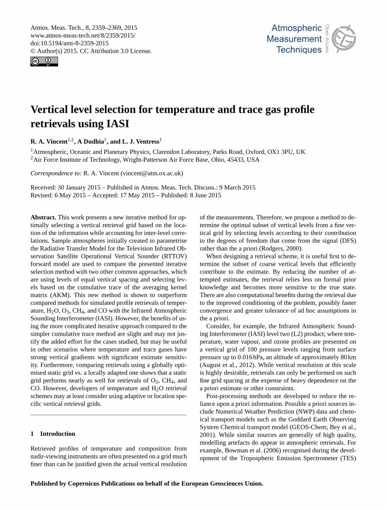
Figure 1. AKM columns are plotted for a sample temperature re-

trieval with IASI using a fine vertical grid (black) compared to

a coarser grid (grey) selected using the iterative vertical selection

method. Note that the pressure axis changes from linear to logarith-

mic above 100hPa (dashed line).

3 Profile level selection

From inspection of Eqs. (11) and (12), selecting an appro-

priate vertical grid depends upon three things; (1) the radia-

tive response of the atmosphere, (2) the spectral resolution

and noise characteristics of the observation instrument, in

this case IASI, and (3) the chosen prior covariance matrix,

Sa. Since IASI is already designed and collecting data, the

only free parameter is the prior covariance. Therefore, it is

important to consider that Sa should be decided upon before

attempting to optimise a retrieval grid.

When determining a coarse retrieval grid the number and

location of profile levels can be chosen in an ad hoc man-

ner or decided based upon the distribution of information in

the profile. The DFS is a natural scalar metric of informa-

tion to use when constructing and comparing different ver-

tical grids, because it can be directly compared to the num-

ber of attempted retrieval levels. When the DFS is approxi-

mately equal to the number of levels, then little prior knowl-

edge appears in the estimate. Other possible scalar metrics of

information include the Shannon information content and the

trace of the Fisher information matrix (Rodgers, 2000, ch. 2).

For this particular application the DFS is the most appropri-

ate. With this in mind, three vertical level selection methods

are described, ranging from the simple to the complex.

3.1 Equal spacing

The simplest possible selection method is to segment the at-

mosphere into layers of equal thickness. Levels of equal pres-

sure may be used for better tropospheric sensitivity, or levels

of equal height for stratospheric sensitivity. Nadir-viewing

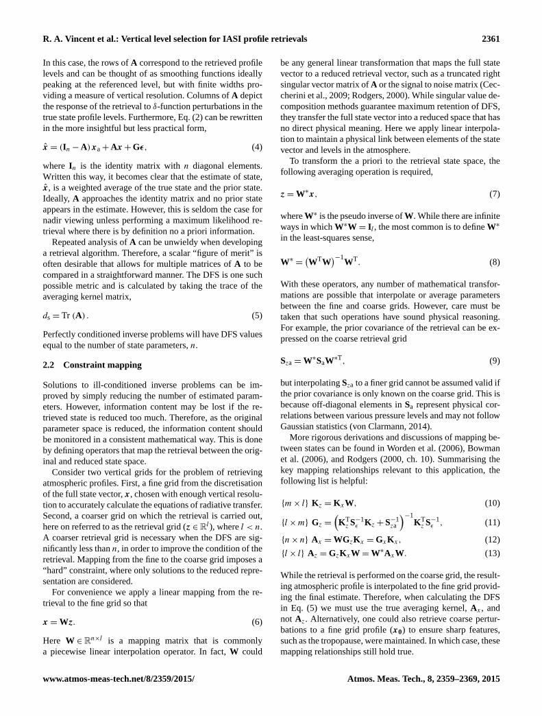
Figure 2. DFS for a temperature retrieval with IASI vs. both ranked

atmospheric pressure levels and ranked spectral channels from the

CO2 spectrum. The black lines show contours of number of pres-

sure levels and the coloured highlight lines show contours of integer

DFS.

instruments such as IASI are typically more sensitive to the

troposphere, so equal pressure spacing will be assumed for

these comparisons, even though it is clearly inappropriate for

species with stratospheric concentrations such as ozone.

3.2 Cumulative trace

Alternatively, a vertical selection method proposed by von

Clarmann and Grabowski (2007) originally for removing

hidden a priori from retrieved estimates is commonly used

(Payne et al., 2009). This method utilises the vertical distri-

bution of the DFS through the profile on the fine grid. From

the averaging kernel matrix, A, the cumulative trace is calcu-

lated as a function of the vertical axis, showing the contribu-

tion of each level to the total DFS of the retrieval. Next, the

cumulative trace is segmented into equal spacings of number

l and the selected coarse vertical levels interpolated from this

curve. The resulting coarse pressure grid is thus irregularly

spaced based on the vertical density of the DFS.

While using the diagonal of A is a clear improvement over

equal pressure spacings, ignoring the off-diagonal sensitivi-

ties is a concern. This is because the original AKM expressed

on the fine grid is likely to change morphology as levels are

combined; hence the impact on the diagonal will not gener-

ally be the simple cumulation assumed. As a result, the ver-

tical partitioning of DFS for a given atmospheric profile re-

trieved over, for example, 100 levels may differ from a 10

level retrieval due to correlations between levels introduced

both spectrally and with Sa. Thus, a vertical selection method

is desired that accounts for off-diagonal changes in Ax dur-

ing the selection process.

Atmos. Meas. Tech., 8, 2359–2369, 2015 www.atmos-meas-tech.net/8/2359/2015/

R. A. Vincent et al.: Vertical level selection for IASI profile retrievals 2363

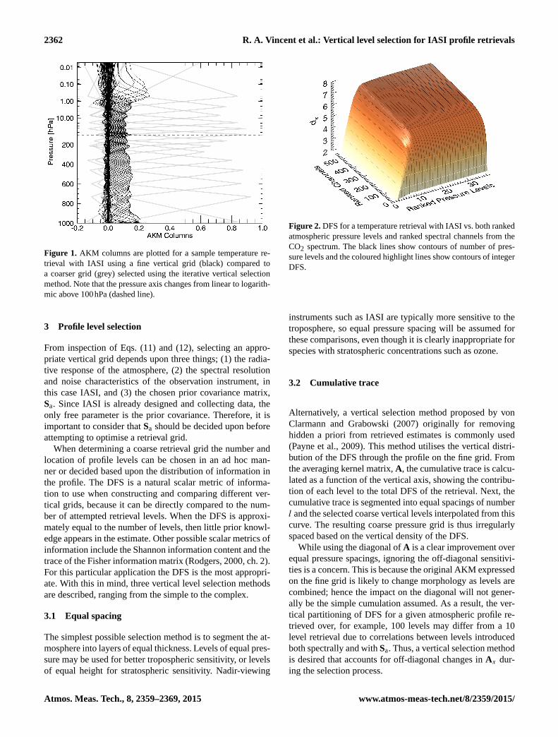
Figure 3. Simulated IASI spectrum showing the spectral ranges

considered in this study, which are typical for temperature and trace

gas profile retrievals with this instrument.

3.3 Iterative selection

The proposed vertical selection method is outlined as fol-

lows.

1. Calculate the DFS on the fine grid by making W= In.

Doing so sets the coarse grid equal to the fine grid.

2. Next, a single level is removed by modifying W in ac-

cordance with the chosen interpolating method. In this

case, the piecewise linear method is used for simplicity.

3. The resulting DFS from removing that level are deter-

mined from Eqs. (12) and (5). Each possible level is re-

moved individually and its effect on the DFS noted. The

removed level that decreased the DFS the least is then

discarded. Removed levels are merged into neighbour-

ing levels by redefining the W matrix.

4. This process is repeated to find the second-least im-

portant level until all vertical levels have been ranked

and discarded down to the two levels that contribute the

most to the DFS.

Following this method results in a ranking of the vertical lev-

els on the fine grid that can be truncated to produce an op-

timal representation on the retrieval grid for any number of

levels.

To visualise the effect, Fig. 1 shows the columns of two

AKMs for a temperature retrieval with IASI using part of the

CO2 spectral feature between 675 and 800 cm−1. The smaller

amplitude responses are for a retrieval on a fine 100 level

pressure grid. While the larger more peaked responses are for

a 15 level grid (ds ≈ 12) chosen using this iterative selection

method. Figure 1 highlights a fundamental trade-off inherent

to constrained retrievals with fixed information content: more

parameters can be retrieved with less sensitivity to the true

state or fewer estimates attempted with greater sensitivity to

the true state.

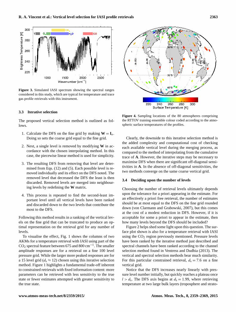
Figure 4. Sampling locations of the 80 atmospheres comprising

the RTTOV training ensemble colour coded according to the atmo-

spheric surface temperatures of the profiles.

Clearly, the downside to this iterative selection method is

the added complexity and computational cost of checking

each available vertical level during the merging process, as

compared to the method of interpolating from the cumulative

trace of A. However, the iterative steps may be necessary to

maximise DFS when there are significant off-diagonal sensi-

tivities in A. In the absence of off-diagonal sensitivities, the

two methods converge on the same coarse vertical grid.

3.4 Deciding upon the number of levels

Choosing the number of retrieval levels ultimately depends

upon the tolerance for a priori appearing in the estimate. For

an effectively a priori free retrieval, the number of estimates

should be at most equal to the DFS on the fine grid rounded

down (von Clarmann and Grabowski, 2007), but this comes

at the cost of a modest reduction in DFS. However, if it is

acceptable for some a priori to appear in the estimate, then

how many levels beyond the DFS should be included?

Figure 2 helps shed some light upon this question. The sur-

face plot shown is also for a temperature retrieval with IASI

using the CO2 region previously mentioned. Pressure levels

have been ranked by the iterative method just described and

spectral channels have been ranked according to the channel

selection method found in Ventress and Dudhia (2013). The

vertical and spectral selection methods bear much similarity.

For this particular constrained retrieval, ds = 7.6 on a fine

vertical grid.

Notice that the DFS increases nearly linearly with pres-

sure level number initially, but quickly reaches a plateau once

l > ds. The DFS axis begins at ds = 1.99, where retrieving

temperature at two large bulk layers (troposphere and strato-

www.atmos-meas-tech.net/8/2359/2015/ Atmos. Meas. Tech., 8, 2359–2369, 2015

2364 R. A. Vincent et al.: Vertical level selection for IASI profile retrievals

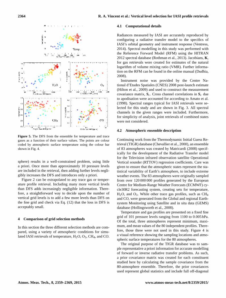
Figure 5. The DFS from the ensemble for temperature and trace

gases as a function of their surface values. The points are colour

coded by atmospheric surface temperature using the colour bar

shown in Fig. 4.

sphere) results in a well-constrained problem, using little

a priori. Once more than approximately 10 pressure levels

are included in the retrieval, then adding further levels negli-

gibly increases the DFS and introduces only a priori.

Figure 2 can be extrapolated to any trace gas or temper-

ature profile retrieval. Including many more vertical levels

than DFS adds increasingly negligible information. There-

fore, a straightforward way to decide upon the number of

vertical grid levels is to add a few more levels than DFS on

the fine grid and check via Eq. (12) that the loss in DFS is

acceptably small.

4 Comparison of grid selection methods

In this section the three different selection methods are com-

pared, using a variety of atmospheric conditions for simu-

lated IASI retrievals of temperature, H2O, O3, CH4, and CO.

4.1 Computational details

Radiances measured by IASI are accurately reproduced by

configuring a radiative transfer model to the specifics of

IASI’s orbital geometry and instrument response (Ventress,

2014). Spectral modelling in this study was performed with

the Reference Forward Model (RFM) using the HITRAN

2012 spectral database (Rothman et al., 2013). Jacobians, K,

for gas retrievals were created for estimates of the natural

logarithm of volume mixing ratio (VMR). Further informa-

tion on the RFM can be found in the online manual (Dudhia,

2008).

Instrument noise was provided by the Centre Na-

tional d’Etudes Spatiales (CNES) 2008 post-launch estimate

(Hilton et al., 2009) and used to construct the measurement

covariance matrix, Sε . Cross channel correlations in Sε due

to apodisation were accounted for according to Amato et al.

(1998). Spectral ranges typical for IASI retrievals were se-

lected for this study and are shown in Fig. 3. All spectral

channels in the given ranges were included. Furthermore,

for simplicity of analysis, joint retrievals of combined states

were not considered.

4.2 Atmospheric ensemble description

Continuing work from the Thermodynamic Initial Guess Re-

trieval (TIGR) database (Chevallier et al., 2000), an ensemble

of 83 atmospheres was created by Matricardi (2008) specif-

ically for the development of the Radiative Transfer model

for the Television infrared observation satellite Operational

Vertical sounder (RTTOV) regression coefficients. Care was

given to ensure that the atmospheric states represent the sta-

tistical variability of Earth’s atmosphere, to include extreme

weather events. The 83 atmospheres were originally sampled

from over 120 000 000 profiles generated by the European

Centre for Medium-Range Weather Forecasts (ECMWF) cy-

cle30R2 forecasting system, creating sets for temperature,

H2O, and O3. While other trace gas profiles, such as CH4

and CO, were generated from the Global and regional Earth-

system Monitoring using Satellite and in situ data (GEMS)

database (Hollingsworth et al., 2008).

Temperature and gas profiles are presented on a fixed fine

grid of 101 pressure levels ranging from 1100 to 0.005hPa.

Of the total, three atmospheres represent minimum, maxi-

mum, and mean values of the 80 independent profiles. There-

fore, those three were not used in this study. Figure 4 is

a visual reference showing the sampling locations and atmo-

spheric surface temperatures for the 80 atmospheres.

The original purpose of the TIGR database was to sam-

ple representative a priori information for accurate modelling

of forward or inverse radiative transfer problems. As such,

a prior covariance matrix was created for each constituent

studied here by calculating the sample covariance from the

80-atmosphere ensemble. Therefore, the prior covariances

used represent global statistics and include full off-diagonal

Atmos. Meas. Tech., 8, 2359–2369, 2015 www.atmos-meas-tech.net/8/2359/2015/

R. A. Vincent et al.: Vertical level selection for IASI profile retrievals 2365

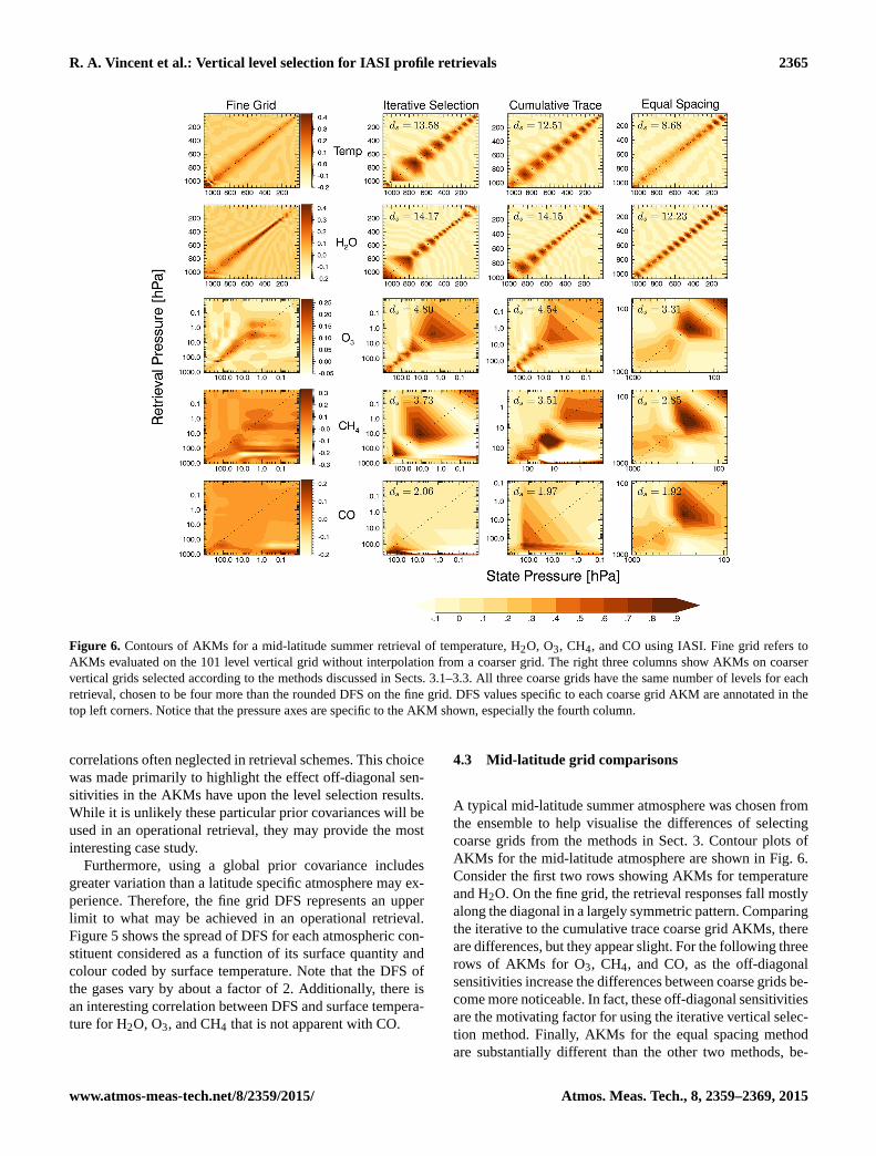
Figure 6. Contours of AKMs for a mid-latitude summer retrieval of temperature, H2O, O3, CH4, and CO using IASI. Fine grid refers to

AKMs evaluated on the 101 level vertical grid without interpolation from a coarser grid. The right three columns show AKMs on coarser

vertical grids selected according to the methods discussed in Sects. 3.1–3.3. All three coarse grids have the same number of levels for each

retrieval, chosen to be four more than the rounded DFS on the fine grid. DFS values specific to each coarse grid AKM are annotated in the

top left corners. Notice that the pressure axes are specific to the AKM shown, especially the fourth column.

correlations often neglected in retrieval schemes. This choice

was made primarily to highlight the effect off-diagonal sen-

sitivities in the AKMs have upon the level selection results.

While it is unlikely these particular prior covariances will be

used in an operational retrieval, they may provide the most

interesting case study.

Furthermore, using a global prior covariance includes

greater variation than a latitude specific atmosphere may ex-

perience. Therefore, the fine grid DFS represents an upper

limit to what may be achieved in an operational retrieval.

Figure 5 shows the spread of DFS for each atmospheric con-

stituent considered as a function of its surface quantity and

colour coded by surface temperature. Note that the DFS of

the gases vary by about a factor of 2. Additionally, there is

an interesting correlation between DFS and surface tempera-

ture for H2O, O3, and CH4 that is not apparent with CO.

4.3 Mid-latitude grid comparisons

A typical mid-latitude summer atmosphere was chosen from

the ensemble to help visualise the differences of selecting

coarse grids from the methods in Sect. 3. Contour plots of

AKMs for the mid-latitude atmosphere are shown in Fig. 6.

Consider the first two rows showing AKMs for temperature

and H2O. On the fine grid, the retrieval responses fall mostly

along the diagonal in a largely symmetric pattern. Comparing

the iterative to the cumulative trace coarse grid AKMs, there

are differences, but they appear slight. For the following three

rows of AKMs for O3, CH4, and CO, as the off-diagonal

sensitivities increase the differences between coarse grids be-

come more noticeable. In fact, these off-diagonal sensitivities

are the motivating factor for using the iterative vertical selec-

tion method. Finally, AKMs for the equal spacing method

are substantially different than the other two methods, be-

www.atmos-meas-tech.net/8/2359/2015/ Atmos. Meas. Tech., 8, 2359–2369, 2015

2366 R. A. Vincent et al.: Vertical level selection for IASI profile retrievals

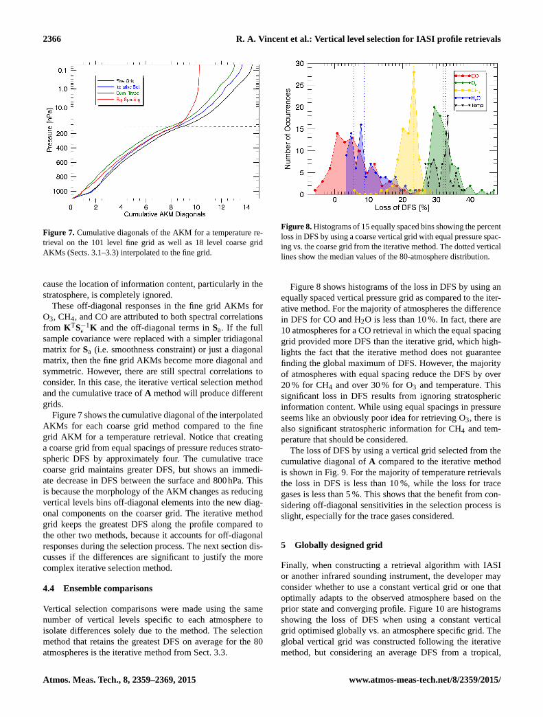
Figure 7. Cumulative diagonals of the AKM for a temperature re-

trieval on the 101 level fine grid as well as 18 level coarse grid

AKMs (Sects. 3.1–3.3) interpolated to the fine grid.

cause the location of information content, particularly in the

stratosphere, is completely ignored.

These off-diagonal responses in the fine grid AKMs for

O3, CH4, and CO are attributed to both spectral correlations

from KTS−1ε K and the off-diagonal terms in Sa. If the full

sample covariance were replaced with a simpler tridiagonal

matrix for Sa (i.e. smoothness constraint) or just a diagonal

matrix, then the fine grid AKMs become more diagonal and

symmetric. However, there are still spectral correlations to

consider. In this case, the iterative vertical selection method

and the cumulative trace of A method will produce different

grids.

Figure 7 shows the cumulative diagonal of the interpolated

AKMs for each coarse grid method compared to the fine

grid AKM for a temperature retrieval. Notice that creating

a coarse grid from equal spacings of pressure reduces strato-

spheric DFS by approximately four. The cumulative trace

coarse grid maintains greater DFS, but shows an immedi-

ate decrease in DFS between the surface and 800hPa. This

is because the morphology of the AKM changes as reducing

vertical levels bins off-diagonal elements into the new diag-

onal components on the coarser grid. The iterative method

grid keeps the greatest DFS along the profile compared to

the other two methods, because it accounts for off-diagonal

responses during the selection process. The next section dis-

cusses if the differences are significant to justify the more

complex iterative selection method.

4.4 Ensemble comparisons

Vertical selection comparisons were made using the same

number of vertical levels specific to each atmosphere to

isolate differences solely due to the method. The selection

method that retains the greatest DFS on average for the 80

atmospheres is the iterative method from Sect. 3.3.

Figure 8. Histograms of 15 equally spaced bins showing the percent

loss in DFS by using a coarse vertical grid with equal pressure spac-

ing vs. the coarse grid from the iterative method. The dotted vertical

lines show the median values of the 80-atmosphere distribution.

Figure 8 shows histograms of the loss in DFS by using an

equally spaced vertical pressure grid as compared to the iter-

ative method. For the majority of atmospheres the difference

in DFS for CO and H2O is less than 10 %. In fact, there are

10 atmospheres for a CO retrieval in which the equal spacing

grid provided more DFS than the iterative grid, which high-

lights the fact that the iterative method does not guarantee

finding the global maximum of DFS. However, the majority

of atmospheres with equal spacing reduce the DFS by over

20 % for CH4 and over 30 % for O3 and temperature. This

significant loss in DFS results from ignoring stratospheric

information content. While using equal spacings in pressure

seems like an obviously poor idea for retrieving O3, there is

also significant stratospheric information for CH4 and tem-

perature that should be considered.

The loss of DFS by using a vertical grid selected from the

cumulative diagonal of A compared to the iterative method

is shown in Fig. 9. For the majority of temperature retrievals

the loss in DFS is less than 10 %, while the loss for trace

gases is less than 5 %. This shows that the benefit from con-

sidering off-diagonal sensitivities in the selection process is

slight, especially for the trace gases considered.

5 Globally designed grid

Finally, when constructing a retrieval algorithm with IASI

or another infrared sounding instrument, the developer may

consider whether to use a constant vertical grid or one that

optimally adapts to the observed atmosphere based on the

prior state and converging profile. Figure 10 are histograms

showing the loss of DFS when using a constant vertical

grid optimised globally vs. an atmosphere specific grid. The

global vertical grid was constructed following the iterative

method, but considering an average DFS from a tropical,

Atmos. Meas. Tech., 8, 2359–2369, 2015 www.atmos-meas-tech.net/8/2359/2015/

R. A. Vincent et al.: Vertical level selection for IASI profile retrievals 2367

Figure 9. Histograms of 15 equally spaced bins showing the percent

loss in DFS by creating a coarse vertical grid from the cumulative

trace of A vs. the coarse grid from the iterative method. The dotted

vertical lines show the median values of the 80-atmosphere distri-

bution.

Table 1. Summaries of the ensemble results from Figs. 8–10. The

second column shows the ensemble mean DFS for each retrieval

using the iterative method. The last three columns show the median

percent loss of DFS for the histograms displayed.

Eq PRE Diag(A) Global

Retrieval ds [%loss] [%loss] [%loss]

Temperature 15.7 32.6 8.6 12.1

H2O 13.8 8.7 1.5 12.1

O3 5.1 32.0 4.2 2.5

CH4 3.8 23.1 3.8 2.1

CO 2.9 5.8 2.5 2.3

mid-latitude, polar summer, and polar winter atmosphere as

the metric of quality.

Notice that the median DFS losses are less than 3 % for

O3, CH4, and CO. However, there are long tails extending

past 10 % for the more extreme atmospheres. Additionally,

temperature and H2O show DFS loss values between 10

and 20 %, suggesting that the vertical location of informa-

tion varies more significantly than the other gases considered.

Therefore, an adaptive atmosphere specific vertical grid may

improve retrievals of temperature and water vapour from an

information perspective. However, the practicalities of im-

plementing an adaptive grid may make this increase in DFS

an undesirable trade-off when attempting to produce time av-

eraged or cross-platform analyses.

To summarise Figs. 8–10, the ensemble median values are

shown in Table 1 along with the mean DFS values for the

referenced iterative selection method.

Figure 10. Histograms of 15 equally spaced bins showing the loss

in DFS by using a constant globally optimised vertical grid vs. an

atmosphere specific grid. The dotted vertical lines show median val-

ues of the 80-atmosphere distribution, where the temperature and

H2O medians overlay each other.

6 Conclusions

When retrieving atmospheric profiles of temperature and

trace gases from infrared spectral radiances, it is important to

consider where in the vertical profile the estimates are made.

A new iterative method for selecting a vertical grid was pro-

posed and shown to outperform previously used selection

methods by accounting for correlations and sensitivities be-

tween different vertical levels. Other compared methods of

establishing a vertical grid coarser than the radiative transfer

grid were using levels equally spaced in pressure and select-

ing levels by interpolating along the cumulative diagonal of

the fine grid AKM.

The 80-atmosphere ensemble created to parametrise RT-

TOV was used to systematically compare the different ver-

tical grid selection methods for temperature, H2O, O3, CH4,

and CO. For the majority of atmospheres, using a vertical

grid with equal pressure spacings resulted in a 20–40 % loss

of DFS for temperature, O3, and CH4. Median DFS losses

for H2O and CO were less than 10 %. In general, this shows

that a significant proportion of DFS can be retained by con-

sidering the vertical location of the information content as

opposed to choosing a vertical grid based on convenience.

Comparing to the cumulative diagonal of A method shows

that greater DFS can be achieved with the iterative method,

but median losses are less than 5 % for the trace gases and

less than 10 % for temperature retrievals. This slight reduc-

tion in DFS is unlikely to affect the quality of retrievals

in a noticeable way for the majority of atmospheric cases.

Therefore, the simpler and less expensive method of inter-

polating along the cumulative diagonal of A will likely be

sufficient, except for possibly extreme atmospheric scenarios

with high inter-level correlations.

www.atmos-meas-tech.net/8/2359/2015/ Atmos. Meas. Tech., 8, 2359–2369, 2015

2368 R. A. Vincent et al.: Vertical level selection for IASI profile retrievals

Finally, much effort is spent making retrieval schemes run

faster. Naturally, one would prefer to design a coarse verti-

cal grid just once and apply that to all scenarios, rather than

optimise a grid for each retrieved atmosphere. This depends

upon the variability of vertical information content. The me-

dian loss of DFS for O3, CH4, and CO when using a globally

optimised grid vs. an atmosphere specific grid was less than

3 %. For the majority of atmospheres, using a static grid re-

sults in a negligible retrieval difference for these three gases.

However, the loss of DFS for temperature and H2O is more

appreciable, greater than 10 %, implying the location of ver-

tical information is more variable than the other trace gases

considered. Whether or not to account for information vari-

ability with temperature and H2O ultimately depends upon

the motivation for computation speed and tolerance of the

DFS reductions presented.

Acknowledgements. Portions of this work were funded by the

United States Air Force. The views expressed in this article are

those of the author and do not reflect the official policy or position

of the United States Air Force, Department of Defense or the US

Government.

Edited by: A. Butz

References

Amato, U., De Canditiis, D., and Serio, C.: Effect of apodization on

the retrieval of geophysical parameters from Fourier-transform

spectrometers, Appl. Optics, 37, 6537–6543, 1998.

August, T., Klaes, D., Schlüssel, P., Hultberg, T., Crapeau, M., Ar-

riaga, A., O’Carroll, A., Coppens, D., Munro, R., and Calbet, X.:

IASI on Metop-A: operational level 2 retrievals after five years

in orbit, J. Quant. Spectrosc. Ra., 113, 1340–1371, 2012.

Aumann, H., Chahine, M., Gautier, C., Goldberg, M., Kalnay, E.,

McMillin, L., Revercomb, H., Rosenkranz, P., Smith, W.,

Staelin, D., Strow, L., and Susskind, J.: AIRS/AMSU/HSB on

the Aqua mission: Design, science objectives, data products,

and processing systems, IEEE T. Geosci. Remote, 41, 253–264,

2003.

Bey, I., Jacob, D. J., Yantosca, R. M., Logan, J. A., Field, B. D.,

Fiore, A. M., Li, Q., Liu, H. Y., Mickley, L. J., and

Schultz, M. G.: Global modeling of tropospheric chemistry with

assimilated meteorology: model description and evaluation, J.

Geophys. Res.-Atmos., 106, 23073–23095, 2001.

Bowman, K. W., Rodgers, C. D., Kulawik, S. S., Worden, J.,

Sarkissian, E., Osterman, G., Steck, T., Lou, M., Eldering, A.,

Shephard, M., Brown, P., Rinsland, C., Gunson, M., and Beer, R.:

Tropospheric emission spectrometer: retrieval method and error

analysis, IEEE T. Geosci. Remote, 44, 1297–1307, 2006.

Brasseur, G., Hauglustaine, D., Walters, S., Rasch, P., Müller, J.-F.,

Granier, C., and Tie, X.: MOZART, a global chemical transport

model for ozone and related chemical tracers: 1. Model descrip-

tion, J. Geophys. Res.-Atmos., 103, 28265–28289, 1998.

Ceccherini, S., Raspollini, P., and Carli, B.: Optimal use of the infor-

mation provided by indirect measurements of atmospheric verti-

cal profiles, Opt. Express, 17, 4944–4958, 2009.

Chevallier, F., Chédin, A., Chéruy, F., and Morcrette, J.-J.: TIGR-

like atmospheric-profile databases for accurate radiative-flux

computation, Q. J. Roy. Meteor. Soc., 126, 777–785, 2000.

Dudhia, A.: Reference Forward Model (RFM), available at: http:

//www.atm.ox.ac.uk/RFM (last access: January 2015), 2008.

Han, Y., Revercomb, H., Cromp, M., Gu, D., Johnson, D.,

Mooney, D., Scott, D., Strow, L., Bingham, G., Borg, L.,

Chen, Y., DeSlover, D., Esplin, M., Hagan, D., Jin, X., Knute-

son, R., Motteler, H., Predina, J., Suwinski, L., Taylor, J., To-

bin, D., Tremblay, D., Wang, C., Wang, L., Wang, L., and Za-

vyalov, V.: Suomi NPP CrIS measurements, sensor data record

algorithm, calibration and validation activities, and record data

quality, J. Geophys. Res.-Atmos., 118, 12734–12748, 2013.

Hilton, F., Atkinson, N., English, S., and Eyre, J.: Assimilation of

IASI at the Met Office and assessment of its impact through ob-

serving system experiments, Q. J. Roy. Meteor. Soc., 135, 495–

505, 2009.

Hollingsworth, A., Engelen, R., Benedetti, A., Dethof, A., Flem-

ming, J., Kaiser, J., Morcrette, J., Simmons, A., Textor, C.,

Boucher, O., Chevallier, F., Rayner, P., Elbern, H., Eskes, H.,

Granier, C., Peuch, V.-H., Rouil, L., and Schultz, M. G.: Toward

a monitoring and forecasting system for atmospheric composi-

tion: the GEMS project, B. Am. Meteorol. Soc., 89, 1147–1164,

2008.

Joiner, J. and Da Silva, A.: Efficient methods to assimilate remotely

sensed data based on information content, Q. J. Roy. Meteor.

Soc., 124, 1669–1694, 1998.

Kulawik, S. S., Osterman, G., Jones, D. B., and Bowman, K. W.:

Calculation of altitude-dependent Tikhonov constraints for TES

nadir retrievals, IEEE T. Geosci. Remote, 44, 1334–1342, 2006.

Matricardi, M.: The generation of RTTOV regression coefficients

for IASI and AIRS using a new profile training set and a new

line-by-line database, ECMWF Research Dept, Reading, UK,

Tech. rep., Tech. Memo., 564, available at: http://www.ecmwf.

int/publications (last access: February 2015), 2008.

Payne, V. H., Clough, S. A., Shephard, M. W., Nassar, R., and Lo-

gan, J. A.: Information-centered representation of retrievals with

limited degrees of freedom for signal: application to methane

from the Tropospheric Emission Spectrometer, J. Geophys. Res.,

114, D10307, doi:10.1029/2008JD010155, 2009.

Rodgers, C. D.: Inverse Methods for Atmospheric Sounding: The-

ory and Practice, vol. 2, World Scientific, Singapore, 2000.

Rothman, L., Gordon, I., Babikov, Y., et al.: The HITRAN2012

molecular spectroscopic database, J. Quant. Spectrosc. Ra., 130,

4–50, 2013.

Ventress, L.: Atmospheric sounding using IASI, PhD thesis, Oxford

University, Oxford, 2014.

Atmos. Meas. Tech., 8, 2359–2369, 2015 www.atmos-meas-tech.net/8/2359/2015/

R. A. Vincent et al.: Vertical level selection for IASI profile retrievals 2369

Ventress, L. and Dudhia, A.: Improving the selection of IASI chan-

nels for use in numerical weather prediction, Q. J. Roy. Meteor.

Soc., 140, 2111–2118, doi:10.1002/qj.2280, 2013.

von Clarmann, T.: Smoothing error pitfalls, Atmos. Meas. Tech., 7,

3023–3034, doi:10.5194/amt-7-3023-2014, 2014.

von Clarmann, T. and Grabowski, U.: Elimination of hidden a priori

information from remotely sensed profile data, Atmos. Chem.

Phys., 7, 397–408, doi:10.5194/acp-7-397-2007, 2007.

Worden, J., Bowman, K., Noone, D., Beer, R., Clough, S., Elder-

ing, A., Fisher, B., Goldman, A., Gunson, M., Herman, R., Ku-

lawik, S. S., Lampel, M., Luo, M., Osterman, G., Rinsland, C.,

Rodgers, C., Sander, S., Shephard, M., and Worden, H.: Tropo-

spheric Emission Spectrometer observations of the tropospheric

HDO/H2O ratio: Estimation approach and characterization, J.

Geophys. Res., 111, D16309, doi:10.1029/2005JD006606, 2006.

www.atmos-meas-tech.net/8/2359/2015/ Atmos. Meas. Tech., 8, 2359–2369, 2015