Very high-frequency radar mapping of surface currents - Oceanic...

IEEE JOURNAL OF OCEANIC ENGINEERING, VOL. 27, NO. 2, APRIL 2002 155

Very High-Frequency Radar Mapping ofSurface Currents

Lynn K. Shay, Thomas M. Cook, Hartmut Peters, Arthur J. Mariano, Robert Weisberg, P. Edgar An,Alexander Soloviev, and Mark Luther

Abstract—An ocean surface current radar (OSCR) in thevery high frequency (VHF) mode was deployed in South FloridaOcean Measurement Center (SFOMC) during the summer of1999. During this period, a 29-d continuous time series of vectorsurface currents was acquired starting on 9 July 1999 and ending7 August 1999. Over a 20-min sample interval, the VHF radarmapped coastal ocean currents over a 7.5 km 8 km domainwith a horizontal resolution of 250 m at 700 grid points. A totalof 2078 snapshots of the two-dimensional current vectors wereacquired during this time series and of these samples, only 69samples (3.3%) were missing from the time series. During thisperiod, complex surface circulation patterns were observed thatincluded coherent, submesoscale vortices with diameters of 2 to3 km inshore of the Florida Current. Comparisons to subsurfacemeasurements from moored and ship-board acoustic Dopplercurrent profiles revealed regression slopes of close to unity withbiases ranging from 4 to 8 cm s 1 between surface and subsurfacemeasurements at 3 to 4 m beneath the surface. Correlation coef-ficients were 0.8 or above with phases of 10 to 20 suggestiveof an anticylconic veering of current with depth relative to thesurface current. The radar-derived surface current field providedspatial context for an observational network using mooring-, ship-and autonomous underwater vehicle-sensor packages that weredeployed at the SFOMC.

Index Terms—ADCP, coastal ocean circulation, current profiles,surface currents, VHF radar, vortices.

I. INTRODUCTION

A CCURATE measurement of ocean surface currents hasbeen one of the more elusive phenomena to confront

ocean scientists. Given increased national attention to thecoastal ocean and in the planned networking of coastal oceanobservatories, the acquisition of the highest quality surfacecurrent data is required to provide spatial context for theemerging suites ofin situ instrumentation. Furthermore,long-term monitoring of the surface circulation would provideimportant data to study its impact on societally relevant issuessuch as search and rescue operations, coastal pollution fromsewage plants, transport of harmful algae blooms, oil spills and

Manuscript received December 18, 2000; revised October 15, 2001.This work was supported by the Ocean Modeling Program under GrantN00014-98-1-0818.

L. K. Shay, T. M. Cook, H. Peters and A. J. Mariano are with the Divisionof Meteorology and Physical Oceanography, Rosenstiel School of Marine andAtmospheric Science, University of Miami, Miami, FL 33149 USA (e-mail:[email protected]).

R. Weisberg and M. Luther are with the Department of Marine Science, Uni-versity of South Florida, St. Petersburg, FL 33701 USA.

P. E. An is with the Division of Ocean Engineering, Florida Atlantic Univer-sity, Dania Beach, FL 33004 USA.

A. Soloviev is with the Department of Oceanography, NOVA SoutheasternUniversity, Dania Beach, FL 33004 USA.

Publisher Item Identifier S 0364-9059(02)03374-5.

its mitigation, beach erosion and renourishment, and air–seainteraction studies.

One of the more promising techniques that has evolved overthe past four decades is the Doppler radar technique [1]. Radarsignals are backscattered from the moving ocean surface by res-onant surface waves of one-half the incident radar wavelength.This Bragg scattering effect results in two discrete peaks in theDoppler spectrum [2]. In the absence of a surface current, spec-tral peaks are symmetric about the Bragg frequency () offsetfrom the origin by an amount proportional to 2 , whererepresents the linear phase speed of the surface wave andisthe radar wavelength. If there is an underlying surface current,Bragg peaks in the Doppler spectra are displaced by an amountof , where is the radial component of cur-rent along the direction of the radar. Thus, to resolve the two-di-mensional (2-D) current fields, two radar stations are requiredwhere their separation determines the domain of the mapped re-gion. While the accuracy of the measurement is a maximum foran angle of intersection of 90between the two radar beams, theerror in resolving the current vectors increases as the intersec-tion angle departs from this optimal value.

The concept of using high frequency (HF) and very highfrequency (VHF) radar pulses to probe ocean surface currentshas received considerable attention in coastal oceanographic ex-periments in Europe and the United States [3], [4]. The twosystems that have been used are the Coastal Ocean DynamicsApplications Radar (CODAR) [5] and the Ocean Surface Cur-rent Radar (OSCR) [6], [7]. More recently, a WEllen RAdar(WERA) system has been developed that also utilizes phased-array technology [8]. While all these systems are based on res-onant Bragg backscatter, there is a fundamental difference inthe methodology used to isolate the ocean area where scatteringoccurs. The OSCR system utilizes an 85-m-long 16- (HF) or32- (VHF) element phased-array antennae to achieve a narrowbeam, electronically steered over the illuminated ocean area(Table I). The beamwidth is a function of the radar wavelengthdivided by the length of the phased array, which is 7for the HFmode and 3.5 for VHF mode. By contrast, CODAR utilizesa three-element crossed-loop/monopole antennae system anddirection-finding techniques that are easily deployed in small,confined areas compared to the beach real estate required forthe length of the phased array. The azimuthal resolution of thecurrent field is based on a least-squares fit of the Fourier seriesto the data [9]. Thus, the current resolution tends to be more sen-sitive to beam patterns in direction-finding algorithms.

In a comprehensive review of the HF radar issues [3], theoret-ical and observed beam patterns were compared for a 16-element

0364-9059/02$17.00 © 2002 IEEE

156 IEEE JOURNAL OF OCEANIC ENGINEERING, VOL. 27, NO. 2, APRIL 2002

phasedarray.Forabeamsteeredat22relativetothephasedarray,observed side lobes in the beam pattern were typically 20–25 dBless than theoretical side lobes in the beam pattern. Observed andtheoretical peaks were equal at 22, suggesting that the surfacecurrent measurements were well resolved. As all HF-radar an-tennaesystemshaveacharacteristicbeampattern,environmentalfactors such as salinity and moisture and path length from theantennae to the sea influence the beam pattern. In addition, forlarger phased arrays, the beach terrain may under some condi-tions constrain the angle of the boresite, which directly impactsthe beam intersectionangles and the resolutionof the surface cur-rent vector. Within this framework, phased array systems (i.e.,OSCR,WERA) tomeasuresurfacecurrents tend tobemorehard-ware intensive whereas crossed-looped monopole antennae sys-tems (i.e., CODAR) requires more software manipulations to de-termine current speed and direction.

While HF-radar techniques to measure surface currentshave existed for several years, little attention has focused onthe comparisons to conventional oceanographic measurementtechniques, except for tidal bands [6], [10]. Recently, surfacecurrents have been compared to subsurface currents from bothfixed and moving platforms during a series of experimentsusing phased-array technology [7], [11]–[14]. Point-by-pointcomparisons have revealed both similarities and differencesbetween surface and subsurface current signals. For example,rms differences have ranged between 7 to 15 cms dependingon the depth of the subsurface measurement. In the NSF andONR sponsoredDuck94experiment, comparisons to a vectormeasuring current meter (VMCM) at 4 m beneath the surfaceindicated an rms difference of 7 cms over a range of 1m s current from a 29-d time series. Given the VMCM’smeasurement accuracy of about 2 cms [15], the accuracy forthe surface currents was about 5 cms , consistent with themanufacturer’s cited values (see Table I). Although differencesstill remain, radar-derived surface current measurementsrepresent the integral of currents in the top meter (or less) ofthe water column ( ) [2] where winds and waves impactsurface currents and near-surface shears. An important issueemerging from recent radar studies is that mooring data repre-sents a point measurement whereas radar-derived estimates areaveraged over areas with dimensions of 0.6 to 4 kmfor theVHF and HF radars, respectively.

In the VHF mode ( 49.95 MHz), comparisons to subsur-face measurements have been generally lacking due in part to itsunder utilization in coastal experimentation. In the VHF modeof OSCR, the radar wavelength is 5.9 m corresponding to aBragg wavelength of 2.95 m. The highest spatial resolution forthis mode is 250 m, which makes the use of VHF radar partic-ularly attractive for bays and ports as well as monitoring sur-face circulation around sewage effluent regions [16]. Measure-ments from a 3-month deployment of a VHF profiler in the equa-torial Pacific Ocean revealed complex surface current patternsthat contained both short- and long-time scale variability [17].Recent surface current observations using VHF radar revealedcomplex surface current patterns in the South Florida OceanMeasurement Center (SFOMC) where coherent, submesoscalevortices had diameters of 2 to 3 km just inshore of the FloridaCurrent (FC) [18]. These high-resolution surface current obser-

TABLE IRSMAS OSCR SYSTEM CAPABILITIES AND

SPECIFICATIONSFOR THEVHF MODE

vations provided spatial context for autonomous underwater ve-hicles (AUVs), a series of upward-looking acoustic Doppler cur-rent profiler (ADCP) from moorings and ship-based ADCP andconductivity-temperature-depth (CTD) measurements (Fig. 1).This experimental approach provided a multiple-scale nestingof relevant submesoscale variability in a coastal ocean subjectto large relative vorticity changes across the shelf break asso-ciated with FC intrusions [19]. The longer-term significance ofthis approach provides a strategy for coastal ocean studies forthe planned networking of observatories using emerging mea-surement technologies.

In the following manuscript, these surface current observa-tions from VHF radar are described and used to characterizethe coastal ocean environment at the SFOMC. Measurementsfrom both moored and ship-board ADCPs are directly comparedto these surface velocity measurements to establish the levelof consistency between observing platforms. During quiescentatmospheric conditions, this approach provided data to examinethe temporally evolving spatial current patterns at unprecedentedresolution just inshore of the FC. Accordingly, the experimentaldesign using the VHF radar is described in Section II. Prevailingcoastal conditions are given in Section III. In Section IV, adetailed comparison is given between surface observations andmoored and ship-based ADCP’s from July 1999 experiment.Results are discussed in Section V with concluding remarks.

II. VHF RADAR MEASUREMENTS

An experiment was conducted in the summer of 1999 in theSFOMC. In this section, the VHF radar approach is describedwithin the context of experimental design and spectral dataquality of the observed surface current signals.

SHAY et al.: VHF RADAR MAPPING OF SURFACE CURRENTS 157

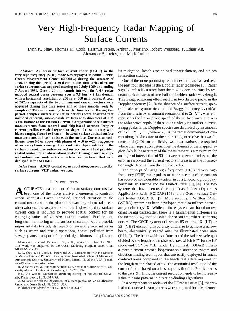
Fig. 1. VHF radar domain (circles) relative to USF/NOVA ADCP moorings (triangles: 50-m mooring at cell 244 is depicted as a red triangle), US navy ADCPs(boxes), and ship track (heavy black line). Inset provides the sampling positions of the ship from five cruises during the month-long experiment. Bottom topographyis contoured at 10-m intervals to 50 m, then contoured at 50 m thereafter. Master and slave sites (heavy solid circles) were located at John U. Lloyd State Park andHollywood Beach, respectively.

A. Experimental Design

The OSCR radar system was deployed in the SFOMC for afour-dimensional ocean current experiment starting on 25 Juneand ending 10 August 1999. During this period, a 29-d contin-uous time series of vector surface currents was acquired startingon 9 July and ending 7 August 1999 at 20-min intervals. Thesystem consisted of two VHF radar transmit/receive stations op-erating at 49.945 MHz that sensed the electromagnetic signalsscattered from surface gravity waves with wavelengths of 2.95m. The VHF radar system mapped coastal ocean currents overa 7.5 km 8 km domain with a horizontal resolution of 250m at 700 grid points (Fig. 1). Radar sites were located in JohnU. Lloyd State Park (adjacent to the US Navy Surface WeaponsCenter Facility) (master: N, W) and an ocean-front site in Hollywood Beach, FL (slave: N, W),equating to a baseline distance of 6.7 km. Each site consistedof a four-element transmit and thirty-element receiving array(spaced 2.95 m apart) oriented at an angle of 37(SW-NE atmaster) and 160(SE-NW at slave).

Effective ranges of the HF and VHF modes of this pulsedradar differ significantly. As shown in Table I, the pulse repe-tition rates ( ) is 80 s and pulse duration for pulses ( )in VHF mode is 1.667 s. Accordingly, the estimated effectiverange is

(1)

where is the speed of light (2.999810 m s ) [20]. For ex-ample, the VHF mode range is approximately 11 km while theeffective range for the HF mode (25.4 MHz) is 44 km for thepresent OSCR configuration. These effective values are also im-portant to the baseline separation distances. In the VHF mode,the baseline distances must be between 3–7 km to optimize theacquisition of the 2-D vector currents. By contrast, separationdistances for an HF mode deployment are typically 20 to 35 kmdepending upon the configuration. In the 1994 Florida Keys ex-periment, for example, the baseline distance was about 38 kmbetween two radar sites [12].


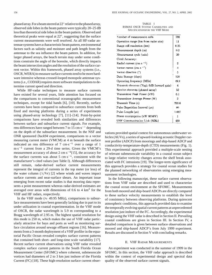
Fig. 2. Doppler spectrum from the 4-D current experiment at cell 300showing the spectral peaks in power (dB) relative to the frequency (Hz). Braggfrequencies are depicted as�� at 0.72 Hz as well as the frequency offset (��).The spectrum was smoothed using a nine point running average correspondingto 0.024 Hz. Frequency offsets of the spectral peaks for the advancing andreceding wave field correspond to the radial current. Second-order returnscontains information about the waves.

B. Bragg Backscatter

The corresponding Bragg frequency is

(2)

where is the acceleration of gravity (9.81 ms ) and ifthe frequency of the radar (49.945 MHz). The resultant Braggfrequency is 0.721 Hz as shown in Fig. 2. Frequency offsetsfrom the first-order Bragg peak ( ) are propor-tional to the radial current for a wave advancing (positive) orreceding (negative) from the radar station (i.e., ,where is the radial component of current along the direc-tion of the radar). Given the range in the Doppler spectrum of

1.5 Hz, the maximum resolvable radial current is4.4ms .In the present context, the maximum current for the FC is ex-pected to be 2 to 2.5 ms , well below this threshold in theDoppler spectrum. Notice that the first-order returns are abovethe noise floor of the Doppler spectra (140 dB) for both ad-vancing and receding waves. To obtain a 2-D vector current atthe 700 cells, two transmit and receive stations are required to re-solve the Doppler spectra as described elsewhere [20] and henceradial current measurements.

C. Radial and Vector Currents

Central to constructing reliable vector current fields from ra-dial measurements is the intersection angle between the radialsemanating from the master and slave stations (Fig. 3). Intersec-tion angles crucially depend on the beach topography, which

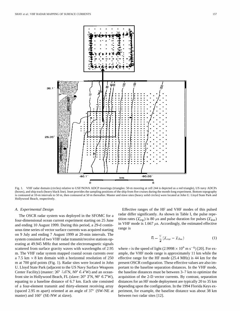
Fig. 3. Intersection angles () between the master and slave radial beams ateach of the 700 OSCR cells. The contour interval is at 10intervals labeled at20 increments.

sets the geometrical constraints of the phased array. In this VHFdomain, optimal intersections angles, defined here as

, encompassed nearly the entire domain except forthe grid points closest to the shore and those just beyond the40 limits in the northeast and southeast corners of the domain.These outer limits were at the maximum range of the master andslave radar stations of 11 km noted above. Thus, physical sig-nificance of the measurements in these areas will be avoided.

The Geometric Dilution Of Precision (GDOP) is used toquanitatively examine the spatial dependence of the observedcurrent differences based on geometrical contraints. Usingthe radar’s mean look direction () and the half-angle ()between intersecting beams [14], expressions for the error inthe along-shelf () and cross-shelf () current components are

(3)

(4)

where represent rms current differences. The GDOP valueis thus defined as the ratios of and for the along-shelf and cross-shelf currents, respectively. Over the VHF radardomain as shown in Fig. 4, the GDOP value ranged from 0.75to 2. In the core of the domain where a large fraction of thesubsurface measurements were acquired, the GDOP for boththe along-shelf () and cross-shelf () currents was unity. Closeto the coast, however, there was a large gradient in the GDOPincreasing from 1 to 2 over a 1.5-2-km (6 to 8 cells) distanceas intersection angles approached the limits (as suggested byFig. 3).

An example of the two radial current plots (master and slave)and the corresponding vector current is shown in Fig. 5. The


Fig. 4. GDOP for the along-shelf (red) and cross-shelf (blue) currents relativeto the cells in the VHF radar domain.

master radial current map indicated a current toward the south-east. On the periphery of this structure, radial currents were di-rected toward the radar site, indicating advancing peaks in theDoppler spectra. Radial currents from the slave station also in-dicated a southwest current in the same regime where masterradial currents were toward the southeast [Fig. 5(b)]. In the cen-tral and southern portions of the VHF radar domain, the radialcurrent field indicated flows in opposite directions with flowstoward and away from the radar over the inner and outer partsof the radar domain, respectively. However, unless radial cur-rents are in the same general directions of the prevailing currentfield, it is difficult to intrepret radial current patterns within thecontext of physical processes. It is more appropriate to convertradial currents to a 2-D current vector consisting of two carte-sian current components.

As each OSCR cell (250 m 250 m) has its own uniquebearing and distance from each site (i.e., Fig. 3), the cross-shelfcurrent at any given cell is

(5)

and the along-shelf current is

(6)

where represent radial currents and represent bearingangles relative to the boresites from the master(m) and slave(s)stations, respectively [21]. As shown in Fig. 5(c), the vector cur-rent field ( ) is constructed from (5) and (6) basedon observed radial currents (5a,b) and bearing angles. For thisparticular snapshot, these data indicated a submesoscale vortex(radius of 1.25 km) rotating cyclonically. Offshore of the vortexwas the inshore edge of the FC where surface currents exceeded

Fig. 5. Maps of a) master radial current, b) slave radial current, and c) vectorcurrent (cm s ) from 0400 GMT 26 June 1999. The scale of the current isgiven in a).

50 cms . Inshore of the vortex, a predominant southward cur-rent of 20 to 30 cms was observed, suggesting fairly compli-cated physical processes over the inner to middle shelf.

D. Spectral Data Quality and Return

Over the course of the experiment, a total of 2078 sampleswas acquired from 0320 GMT 9 July (YearDay 191) until 2340GMT 6 August (YD 220) yielding a 29-d time series. Of the2078 samples, only 69 samples were missing from the vectortime series, equating to a 3.3% loss of the 20 minute snapshots.Previous HF radar experiments have typically yielded data re-turns of 93% to 97% [7], [11], [12]. Thus, these experimental re-sults using the VHF mode were on the higher end of the limitswith respect to overall data return relative to previous experi-mental results.

As shown in [22], the spectral quality index takes into consid-eration: the size of the largest peak (in decibels); the number ofBragg peaks in the spectrum (either 2,1,0); the Bragg ratio (dif-ference between positive Bragg peak and negative Bragg peakin decibels where the smaller the Bragg ratio, the higher thequality number); the width of the largest Bragg peak (the topquality numbers (7,8,9) require that least one Bragg peak spans0.022 Hz in frequency space); and the error in the Bragg peakseparation. This index is an integer in the range of 0 to 9, where9 being the highest quality index. During the course of this ex-periment, this spectral quality index from both the master andslave radar stations ranged between 3 to 7 (Fig. 6). Notice thathigher spectral quality from each site was closest to the coastas signal strength of ground wave signals is a function of bothtransmit frequency and sea water conductivity. As frequencyincreases, transmitted signals attenuate quicker than those oflower frequencies [3]. Of equal importance, the conductivity of


Fig. 6. Spectral quality numbers from a) master and b) slave stations basedupon the spectral data in the Doppler spectra and c) the signal strength (dB)along a radial emanating from the master site (solid line in panel a). Highspectral data quality number corresponds to good separation between thefirst-order peaks and the noise floor and well-defined Bragg ratios. Notice thatin the far-field relative to the master and slave stations (10–11 km) the spectralquality numbers and signal strength decrease to 3 and�120 dB.

the sea surface plays an important role in ground wave propa-gation. As conductivity increases, signal attenuation decreasesexponentially with distance offshore. This is precisely why HFradar techniques attenuate by 40 dB after just a few kilometersover fresh water. Based on CTD measurements from the moor-ings and theR/V Stephan[23], the corresponding conductivitiesexceeded 5.5 m , providing a good conducting plane forground wave propagation. Even in the far-field, typically 10 kmfrom the radar sites, spectral data quality decreased only to 3,which was sufficient to resolve the currents. Along one of theradial legs, the signal-to-noise ratio (SNR), defined as the differ-ence between the strength of the Bragg peak and the noise floor,decreased by about 30 dB from the coast to the far-field [seeFig. 6(c)]. As spectral quality indicies decrease toward unity,current signals cannot be resolved from the Bragg peaks in thespectra and are eliminated from further analysis. Here, as thespectral quality index remained at 3 or above, radar-derived cur-rents were of sufficient quality to warrant a detailed compar-ison to subsurface current observations from the mooring andship-based measurements.

III. OBSERVATIONS

A. Atmospheric Conditions

Prevailing atmospheric conditions during the experimentwere relatively calm as indicated by near-surface wind andpressure records from a Coastal Marine Automated Network(CMAN) station at Fowey Rocks ( N, W), whichwas located approximately 70 km south of the domain. Asshown in Fig. 7, 40-h low-pass filtered surface winds wereonshore ranging between 3 to 7 ms . On YD 202, surfacewinds reversed to a southerly then to an offshore wind as the

Fig. 7. Forty-hour low-pass filtered a) surface wind (m s) and b) surfacepressure (mb) from hourly observations at the CMAN station at Fowey Rockslocated south of the VHF radar domain in July–August 1999. Surface windwas placed into an oceanographic context and then rotated 90cyclonically. Apositive value for the wind represents offshore flows whereas a negative valuerepresents onshore surface winds.

pressure decreased from 1023 to 1012 mb over a 10-d period[Fig. 7(b)]. During this weak pressure change, surface windswere 4 to 6 ms . Averaged over the month time series,the mean wind speed was 4.5 ms directed toward 210T.Meteorological conditions at the Lake Worth CMAN station( N, W, not shown) were similar to these obser-vations from Fowey Rocks. Based upon these data, the meanwind-induced surface current was estimated to be 6 cm sfor an Ekman depth of 30 m. Theoretically, the steady-state,wind-induced surface flows should be directed 45to the rightthe wind; however, in this case, the mean coastal currents weredirected toward the north opposing the mean wind direction.

Surface wave measurements at the NOVA/USF mooring in11 m of water revealed significant wave heights of 1 m or lessduring the first half of July where the surface gravity waves hadperiods between 4–6 s. Based on the deep-water dispersion re-lation, these waves had horizontal wavelengths of about 40 mfor a 5-s wave. The estimated Stokes drift at the surface was5–6 cms for a mean wind speed of 4.5 ms [21]. Given avertical dependence of where is the wavenumber of thedominant wave ( m), the estimated current differencefor this Stokes wave component was less than 1 cms mbetween the surface and 4-m depth. Thus, during the observa-tional period, surface winds and waves did not appear to sig-nificantly impact the surface velocity field compared to oceanicforcing induced by the FC intrusions across the shelf break.

B. Surface Current Observations

An example of the observed surface current variability isshown in Fig. 8 over a 3-d period, including FC intrusions.On 18 July (YD 200), surface velocities exceeded 1.4 msbetween 5 to 7 km offshore with a large surface current gradientnear the shelf break. Closer to the coast, surface currents wereweaker with velocities of 20 to 30 cms . Over the next 8


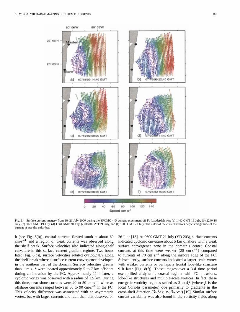
Fig. 8. Surface current imagery from 18–21 July 2000 during the SFOMC 4-D current experiment off Ft. Lauderdale for: (a) 1440 GMT 18 July, (b) 2240 18July, (c) 0020 GMT 19 July, (d) 1140 GMT 20 July, (e) 0600 GMT 21 July, and (f) 1500 GMT 21 July. The color of the current vectors depicts magnitude of thecurrent as per the color bar.

h [see Fig. 8(b)], coastal currents flowed south at about 60cm s and a region of weak currents was observed alongthe shelf break. Surface velocities also indicated along-shelfcurvature in this surface current gradient regime. Two hourslater [Fig. 8(c)], surface velocities rotated cyclonically alongthe shelf break where a surface current convergence developedin the southern part of the domain. Surface velocities greaterthan 1 ms were located approximately 5 to 7 km offshoreduring an intrusion by the FC. Approximately 11 h later, acyclonic vortex was observed with a radius of 1.5 km. Duringthis time, near-shore currents were 40 to 50 cms whereasoffshore currents ranged between 80 to 90 cms in the FC.This velocity difference was associated with an asymmetricvortex, but with larger currents and radii than that observed on

26 June [18]. At 0600 GMT 21 July (YD 203), surface currentsindicated cyclonic curvature about 5 km offshore with a weaksurface convergence zone in the domain’s center. Coastalcurrents at this time were weaker (20 cms ) comparedto currents of 70 cm s along the inshore edge of the FC.Subsequently, surface currents indicated a larger-scale vortexwith weaker currents or perhaps a frontal lobe-like structure9 h later [Fig. 8(f)]. These images over a 3-d time periodexemplified a dynamic coastal regime with FC intrusions,lobe-like structures and multiple-scale vortices. In fact, theseenergetic vorticity regimes scaled as 3 to 4(where is thelocal Coriolis parameter) due primarily to gradients in thecross-shelf direction ( ) [19]. Similar surfacecurrent variability was also found in the vorticity fields along


Fig. 9. a) Time-averaged mean current (arrows) superposed on covariance of the observed surface flows and standard deviations of b) cross-shelf and c) along-shelfsurface currents estimated from the 29-day mean current in a). Color bar depicts the covariance estimates (cm� s ) and standard deviations (cm�s ). Noticethat the along-shelf standard deviation (panel c) is 2 to 5 times larger than in the cross-shelf direction (panel b).

the Florida Keys during an HF radar experiment in May 1994[12].

To further illustrate this spatial surface current variability, thetime-averaged mean, covariance, and standard deviations wereestimated from the 29-d time series (Fig. 9). Time-averagedmean flows were aligned in the along-shelf direction and op-posed the mean surface winds as noted above. Beyond the shelfbreak, northward currents exceeded 50 cms , consistent withthe close proximity of the FC to the coast. Inside the shelf break,mean flows were considerably weaker with currents of 10 to 20cm s , generally directed toward the north. In the central por-tion of the mapped domain, the covariance between the cross-shelf and along-shelf flows revealed an elongated regime wherecovariance estimates were less than100 cm s due in part tothe observed cyclonically rotating vortices and lobe-like struc-tures (i.e., Fig. 8). The covariance between the cross-shelf andalong-shelf currents was positive surrounding this covarianceminima where values exceeded 100 cms along the easternedge of the vortex region. Standard deviations for the cross-shelf[Fig. 9(b)] and the along-shelf [Fig. 9(c)] currents differed by afactor of 2 to 5 depending on their location. For example, alongthe inner and outer edge of this covariance minima, cross-shelfstandard deviations were a maximum of 12 to 14 cms com-pared to 40 and 70 cms in the along-shelf current’s standarddeviation. These time-averaged estimates of the surface currentstatistical properties suggests substantial cross-shelf variabilityin the along-shelf surface current structure, particularly in thevortex-dominated regime. One possibility is that this regime wasdominated by wave-like features [19].

C. Ship-Based Measurements

Ship-based ADCP measurements of horizontal current pro-files with an RDI 5-beam, 600-kHz broad-band ADCP and ofthe stratification with an Ocean Sensors (OS500) CTD were

acquired from theR/V Stephanduring AUV operations. TheADCP was deployed over the starboard side of theR/V Stephan.Shipborne CTD and ADCP measurements were acquired overa rectangular box pattern (see Fig. 1). The eastern, north–southleg of the ship track was positioned beyond the shelf break (co-incident with thethird reef) because high horizontal and verticalshear tended to occur beyond or just east of the shelf break. Thetypical ship speed along the transects was 1.5 ms such thatthe ship track boxes required 1.5 to 3 h to complete.

As shown in Fig. 10, the ADCP was set to 1-m bins, pro-ducing a vertical range of about 35 m depth. Bottom trackingwas possible at depths up to 85 m. Note that all observations(15-s ensemble averages) had valid bottom tracking and dif-ferential GPS (DGPS) navigation data were logged along withthe ADCP output. Two cross-shelf sections of the along-shelfflow indicated the extreme oceanic conditions that frequentlyoccurred in this regime. Relatively weak southward flow wasobserved over the shelf and shelf break at 0400 GMT 16 Julywith weak vertical current shear of 10s . Fifteen hours later(1900 GMT), the FC intruded over the shelf as upper ocean cur-rents increased to 80 cms [upper right edge of Fig. 10b)]although there was still southward flow of 20 cms over theinner-shelf [Fig. 10(b)]. With the FC so close to the shelf, strongvertical shears were also evident in the ADCP measurements.Such flow reversals occurred both on relatively long-time scalesof days and relatively short-time scales of 3, 10, and 27 h. Theseship-board measurements revealed complicated and highly in-termittent FC forcing events across the shelf break that affectedthe coastal circulation.

D. Moored Measurements

The University of South Florida (USF) and NOVA South-eastern University deployed three moored ADCP arrays in theSFOMC as shown in Fig. 1. These profilers sampled the current


Fig. 10. Cross-shelf sections of the along-shelf currents from the shipboard 600 kHz ADCP on theR/V Stephan: (a) 16 July 1999, 0403 GMT and (b) 16 July1999, 1849 GMT. The latitude of the data is 26.053N. Velocity is contoured at 10 cm�s intervals. The zero velocity contour is a heavy, dark line.

structure at 15-min intervals from an upward-looking 300-kHzADCP at the 11-m mooring and two downward-looking600-kHz ADCPs at 20- and 50-m depths. The bin size at the11- and 20-m moorings was set to 0.5 m while a bin size of1 m was used at the 50-m mooring. In addition, microcatswere deployed at both the NE and SW moorings to measuretemperature, conductivity, salinity, and density fields at 5-minintervals at several vertical levels. Data acquisition started on25 June at the 11-m mooring and on 15 July (YD 197) at the NEand SW mooring sites. For the purposes of this manuscript, the50-m mooring ADCP measurements acquired near the center ofthe radar domain will be used in the comparisons below wherethe GDOP was unity in both current directions (see Fig. 4).

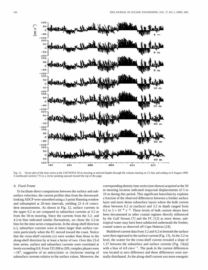
As shown in Fig. 11, coherent structure was observedthroughout the water column in July and early August wherethe current ranged from 50 to 100 cms . Initially, anear-daily oscillatory current of 20 to 30 cms was observedwith larger currents near the surface. Near YD 201, currentsthroughout the column indicated an along-shelf flow of 30cm s toward the south. The current structure then reversedto a predominate, northward along-shelf current until aboutYD 206 when the current became oscillatory with amplitudesexceeding 50 cms . Subsequently, an FC intrusion wasobserved between YD 210 to 213 over the 50-m isobath. Thecurrent during this time was in the along-shelf direction withweak cross-shelf flows. Upper ocean currents approached 100cm s , that decreased to about 40 cms near the bottom.Strong oscillatory currents were also evident after this FCintrusion. Over the 23 days of coincident measurements, thecurrents seemed to bepredominantlybarotropic with relativelyweak cross-shelf flows.

RMS differences between adjacent ADCP bins were exam-ined from 3 to 40 m (not shown) to understand subsurface cur-

rent variability. For the cross-shelf current, bin-to-bin variabilitywas 2 to 3 cms in the upper 10 m, decreasing to 2 cmsat depth. By contrast, bin-to-bin variability was 5 to 7 cmsin the upper 10 m for the along-shelf current, decreasing to 3cm s below 10 m. As suggested by ship-board measurements,this variability is relevant to the comparisons to the surface cur-rents discussed below.

IV. COMPARISONS

Observations described in Section III indicated sufficient ve-racity to warrant a comparison between the radar-derived sur-face signals and subsurface measurements from the ADCP onthe mooring (fixed frame) and theR/V Stephan(moving frame).To place these comparisons into context of other radar deriveddata sets, published analysis techniques will be used to examinethe differences. The difference here is that the spatial resolu-tion of the surface current is now 250 m vice 1.2 km, yieldinga significantly higher resolution surface velocity field that re-solved submesoscale processes. One statistical measure of thecorrelation between two differing measurements is the complexcorrelation coefficient

(7)

and the complex phase angle

(8)

where represents an average (based uponpoints) [23]for the surface () and subsurface () currents. This phase anglerepresents the average cyclonic angle of the subsurface currentvector with respect to the surface current vector.


Fig. 11. Vector plot of the time series at the USF/NOVA 50-m mooring at selected depths through the column starting on 15 July and ending on 8 August 1999.A northward current (T) is a vector pointing upward toward the top of the page.

A. Fixed Frame

To facilitate direct comparisons between the surface and sub-surface velocities, the current profiler data from the downward-looking ADCP were smoothed using a 3-point Hanning windowand subsampled at 20-min intervals, yielding 23 d of coinci-dent measurements. As shown in Fig. 12, surface currents inthe upper 0.2 m are compared to subsurface currents at 3.2 mfrom the 50-m mooring. Since the currents from the 3.2- and4.2-m bins indicated similar fluctuations, we chose the 3.2-mbins for the time series comparisons. In the along-shelf direction( ), subsurface currents were at times larger than surface cur-rents particularly when the FC moved toward the coast. Noticethat the cross-shelf currents () were weaker than those in thealong-shelf direction by at least a factor of two. Over this 23-dtime series, surface and subsurface currents were correlated atlevels exceeding 0.8. From YD 208 to 209, complex phases were

16 , suggestive of an anticyclonic or clockwise veering ofsubsurface currents relative to the surface values. Moreover, the

corresponding density time series (not shown) acquired at the 50m mooring location indicated isopycnal displacements of 5 to10 m during this period. This significant baroclinicity explainsa fraction of the observed differences between a fresher surfacelayer and more dense subsurface layers where the bulk currentshear between 0.2 m (surface) and 3.2 m depth ranged from0.2 to 5 10 s . These levels of bulk current shears havebeen documented in other coastal regimes directly influencedby the Gulf Stream [7] and the FC [12] as more dense, sub-tropical water may have been subducted underneath the fresher,coastal waters as observed off Cape Hatteras [24].

Multilevel current data from 3.2 and 4.2 m beneath the surfacewere then regressed to the surface current (Fig. 13). At the 3.2-mlevel, the scatter for the cross-shelf current revealed a slope of1.37 between the subsurface and surface currents [Fig. 13(a)]with a bias of 4.8 cms . The peak in the current differenceswas located at zero difference and these differences were nor-mally distributed. As the along-shelf current was more energetic


Fig. 12. Comparison of OSCR-derived surface and subsurface (3.2 m) current time series from a downward-looking ADCP attached to a surface mooring alongthe 50 m isobath deployed by USF/NOVA for: (a) along-shelf component (cm s), (b) cross-shelf component (cm�s ), (c) bulk current vector shear (�10 s )defined as the current differences within panels a and b divided by a depth difference of 3 m and (d) daily complex correlation coefficients ( ) and phase angles(�( ): located at the top of the bars) relative to the surface velocity. A negative phase implies an anticyclonic current veering with depth.

than the cross-shelf current, the bias was 8.9 cms with a slopeof unity [Fig. 13(b)]. The frequency distribution in this case sug-gested a slight positive shift of 5 cms in the current differ-ences. Similar results were also apparent in the comparisons at4.2 m where the cross-shelf current bias was 3.8 cms with aslope of 1.31 [Fig. 13(c)]. By contrast, along-shelf current dif-ferences indicated a bias of 8.4 cms again with a slope of 1[Fig. 13(d)]. These results suggest that the measurements in theupper few meters of the water column at the 50-m mooring werequanitatively consistent with surface currents.

Surface velocities at the 50-m mooring (i.e., cell 244 depictedas a red triangle in Fig. 1) were used to estimate the complexcorrelation and phase as per (7) and (8) averaged over the 29-dtime series at each of the radar cells. As shown in Fig. 14, cor-relation coefficients were elongated in the along-shelf direc-tion with a maximum of 1 at the 50 m mooring. Notice themarked spatial change in the correlation coefficient in the cross-shelf direction. Correlation indices decreased by 0.2 kminthe onshore direction, whereas in the offshore direction, thecorrelation coefficient decreased by only 0.1 km. Given thepresence of the FC and its influence on the coastal ocean, thelarger correlation gradient was in the onshore direction. Com-

Fig. 13. Scatter diagrams (left) histograms (right) for the comparisons ofsurface and subsurface currents at the 50-m mooring at 3.2 m (panels a,b) and4.2 m (panels c,d).

plex phase angles ranged from25 in the southwestern portionof the domain compared to 10in the northwestern part of thedomain. The phase angles revealed an anticyclonic veering of


Fig. 14. a) Complex correlation and b) phase () relative to the OSCR cell 244 (red tirangle in Fig. 1) corresponding to the 50 m USF mooring for the 29-d timeseries. The correlation coefficient is contoured at 0.1 intervals and the complex phase is contoured at 2.5increments.

TABLE IIAVERAGED DIFFERENCEBETWEEN THESURFACE AND SUBSURFACECURRENTS

(3 M, 4 M, AND DEPTH-AVERAGED) FOR SPEED(V ), DIRECTION (� ),EAST–WEST (u ) COMPONENT, NORTH–SOUTH (v ) COMPONENT,

COMPLEX CORRELATION COEFFICIENT ( ), PHASE (�) AND THE RMS

DIFFERENCES IN THEEAST–WEST(u ) AND NORTH–SOUTH (v )VELOCITY COMPONENTSBASED ON MOORING AND SHIP TRANSECTDATA

DURING THE JULY 1999 EXPERIMENT AT SFOMC

the current vector except in the northwest quadrant where thephase angle veered in the cyclonic direction relative to the sur-face velocity at 50 m. While the mooring comparisons showedreasonably good correlation indices, the surface velocity struc-ture was highly variable and required cross-shelf measurementsfrom ship, mooring or AUV platforms to resolve submesoscalecurrent structure [18], [19].

Averaged current differences from 23 d of coincident mea-surements are listed in Table II. In terms of current speeds, therewas a 11.7-cms difference between the surface and 3.2-mvalue. This difference decreased to about 8.7 cms at 4.2-mdepth. The difference between the depth-averaged and the sur-face currents was slightly less, suggesting the relative impor-tance of the depth-averaged flows [19]. Similarly, the differ-ences in the current direction were 13 to 14at both 3 and4 m beneath the surface. Regardless of the 3.2-m, 4.2-m, ordepth-averaged comparisons to the surface flow, correlation co-efficients exceeded 0.8 with complex phases of1 to 2 . Ofparticular importance here, rms differences ranged between 13to 22 cms for the velocity components. Given the bin-to-bin

current variability in the ADCP measurements of 3 to 7 cmsin the upper 10 m, these rms differences actually ranged be-tween 10 to 15 cm s , consistent with previous findings. More-over, these rms current differences may not necessarily repre-sent just measurement error. Measurement error for the radar-derived currents has been cited to be between 4–5 cms whilemeasurement error for ADCP-derived currents is 1 to 2 cms .Thus, a large fraction of these differences may be associatedwith the geophysical variability as observed in previous sets ofradar-derived surface current measurements. These VHF radar-derived surface velocities were reliable and reflective of a highlyenergetic coastal regime influenced by the FC at the SFOMC.

B. Moving Frame

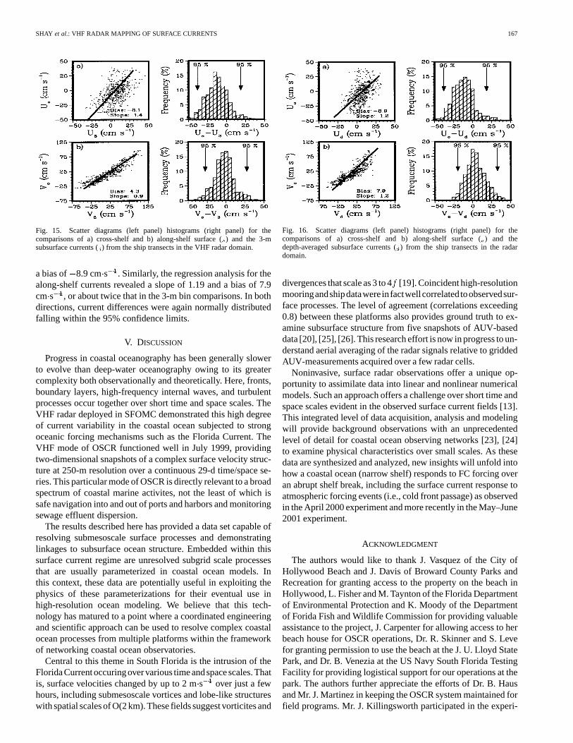
Downward-looking ADCP profiles and CTD measurementsfrom the R/V Stephanwere also acquired during the experi-ment from several days of measurements. Of particular interestis to examine the 3-m bin data and the depth-averaged flows interms of correlating the signals to the radar-derived signals. Theclosest radar measurement in time and space to each ship pro-file was used in these comparisons following [14]. As shownin Fig. 15, comparisons at the 3-m bin revealed similar regres-sion slopes in both the cross-shelf and along-shelf directions.In the cross-shelf direction, for example, the slope was about1.4 with a bias of 8.1 cm s . However, the scatter was muchgreater than that observed at the mooring site as reflected by the10 cms current differences in the histograms. The scatter inthe along-shelf current direction was also much less and moreconsistent with mooring results. For these data, the slope ap-proached unity with a bias of 4.3 cms . In both cases, currentdifferences were normally distributed falling within a 95% con-fidence band as in the mooring data.

Given the relatively shallow depths along the ship transects,the ADCP current profiles were vertically averaged and com-pared to the surface current as shown in Fig. 16. There was lessscatter ( 20 cms ) in the cross-shelf direction than in the 3-mcomparison and the slope of the regression curve was 1.18 with


Fig. 15. Scatter diagrams (left panel) histograms (right panel) for thecomparisons of a) cross-shelf and b) along-shelf surface () and the 3-msubsurface currents () from the ship transects in the VHF radar domain.

a bias of 8.9 cms . Similarly, the regression analysis for thealong-shelf currents revealed a slope of 1.19 and a bias of 7.9cm s , or about twice that in the 3-m bin comparisons. In bothdirections, current differences were again normally distributedfalling within the 95% confidence limits.

V. DISCUSSION

Progress in coastal oceanography has been generally slowerto evolve than deep-water oceanography owing to its greatercomplexity both observationally and theoretically. Here, fronts,boundary layers, high-frequency internal waves, and turbulentprocesses occur together over short time and space scales. TheVHF radar deployed in SFOMC demonstrated this high degreeof current variability in the coastal ocean subjected to strongoceanic forcing mechanisms such as the Florida Current. TheVHF mode of OSCR functioned well in July 1999, providingtwo-dimensional snapshots of a complex surface velocity struc-ture at 250-m resolution over a continuous 29-d time/space se-ries. This particular mode of OSCR is directly relevant to a broadspectrum of coastal marine activites, not the least of which issafe navigation into and out of ports and harbors and monitoringsewage effluent dispersion.

The results described here has provided a data set capable ofresolving submesoscale surface processes and demonstratinglinkages to subsurface ocean structure. Embedded within thissurface current regime are unresolved subgrid scale processesthat are usually parameterized in coastal ocean models. Inthis context, these data are potentially useful in exploiting thephysics of these parameterizations for their eventual use inhigh-resolution ocean modeling. We believe that this tech-nology has matured to a point where a coordinated engineeringand scientific approach can be used to resolve complex coastalocean processes from multiple platforms within the frameworkof networking coastal ocean observatories.

Central to this theme in South Florida is the intrusion of theFloridaCurrentoccuringovervarious timeandspacescales.Thatis, surface velocities changed by up to 2 ms over just a fewhours, including submesoscale vortices and lobe-like structureswith spatial scales of O(2 km). These fields suggest vorticites and

Fig. 16. Scatter diagrams (left panel) histograms (right panel) for thecomparisons of a) cross-shelf and b) along-shelf surface () and thedepth-averaged subsurface currents () from the ship transects in the radardomain.

divergences that scale as 3 to 4[19]. Coincident high-resolutionmooringandshipdatawereinfactwellcorrelatedtoobservedsur-face processes. The level of agreement (correlations exceeding0.8) between these platforms also provides ground truth to ex-amine subsurface structure from five snapshots of AUV-baseddata [20], [25], [26]. This research effort is now in progress to un-derstand aerial averaging of the radar signals relative to griddedAUV-measurements acquired over a few radar cells.

Noninvasive, surface radar observations offer a unique op-portunity to assimilate data into linear and nonlinear numericalmodels. Such an approach offers a challenge over short time andspace scales evident in the observed surface current fields [13].This integrated level of data acquisition, analysis and modelingwill provide background observations with an unprecedentedlevel of detail for coastal ocean observing networks [23], [24]to examine physical characteristics over small scales. As thesedata are synthesized and analyzed, new insights will unfold intohow a coastal ocean (narrow shelf) responds to FC forcing overan abrupt shelf break, including the surface current response toatmospheric forcing events (i.e., cold front passage) as observedin the April 2000 experiment and more recently in the May–June2001 experiment.

ACKNOWLEDGMENT

The authors would like to thank J. Vasquez of the City ofHollywood Beach and J. Davis of Broward County Parks andRecreation for granting access to the property on the beach inHollywood, L. Fisher and M. Taynton of the Florida Departmentof Environmental Protection and K. Moody of the Departmentof Forida Fish and Wildlife Commission for providing valuableassistance to the project, J. Carpenter for allowing access to herbeach house for OSCR operations, Dr. R. Skinner and S. Levefor granting permission to use the beach at the J. U. Lloyd StatePark, and Dr. B. Venezia at the US Navy South Florida TestingFacility for providing logistical support for our operations at thepark. The authors further appreciate the efforts of Dr. B. Hausand Mr. J. Martinez in keeping the OSCR system maintained forfield programs. Mr. J. Killingsworth participated in the experi-


ment as part of a summer internship at RSMAS. Insightful com-ments by the anonymous reviewers improved the manuscript.

REFERENCES

[1] D. D. Crombie, “Doppler spectrum of sea echo at 13.56 Mc. s,” Na-ture, vol. 175, no. 4459, pp. 681–682, 1955.

[2] R. H. Stewart and J. W. Joy, “HF radio measurements of surface cur-rents,”Deep-Sea Res., vol. 21, pp. 1039–1049, 1974.

[3] K.-W. Gurgel, H.-H. Essen, and S. P. Kingsley, “High frequencyradars: limitations and recent developments,”Coastal Eng., vol. 37, pp.201–218, 1999.

[4] J. D. Paduan and H. C. Graber, “Introduction to high frequency radar:Reality and myth,”Oceanography, vol. 10, no. 4, pp. 36–39, 1997.

[5] D. E. Barrick, “First order theory and analysis of MF/HF/VHF scatterfrom the sea,”IEEE Trans. Antennas Propagat., vol. 20, pp. 2–10, 1992.

[6] D. Prandle, “The fine-structure of nearshore tidal and residual circu-lations revealed by HF radar surface current measurements,”J. Phys.Oceanogr., vol. 17, no. 1, pp. 231–245, 1987.

[7] L. K. Shay, H. C. Graber, D. B. Ross, and R. D. Chapman, “Mesoscaleocean surface current structure detected by HF radar,”J. Atmos. Ocean.Technol., vol. 12, no. 4, pp. 881–900, 1995.

[8] K.-W. Gurgel, G. Antonischki, H.-H. Essen, and T. Schlick, “Wellenradar (WERA): a new ground wave HF radar for remote sensing,”Coastal Eng., vol. 37, pp. 219–234, 1999.

[9] B. J. Lipa and D. E. Barrick, “Least-squares methods for the extractionof surface currents from CODAR crossed loop data: Application at AR-SLOE,” IEEE J. Ocean Eng., vol. OE-8, pp. 226–253, 4 1983.

[10] J. D. Paduan and L. K. Rosenfield, “Remotely sensed surface cur-rents in Monterey Bay from shore-based HF radar (Coastal OceanDynamics Application Radar),”J. Geophys. Res., vol. 101, no. 9, pp.20 669–20 686, 1996.

[11] L. K. Shay, S. J. Lentz, H. C. Graber, and B. K. Haus, “Current structurevariations detected by high frequency radar and vector measuring currentmeters,”J. Atmos. Oceanic. Technol., vol. 15, no. 1, pp. 237–256, 1998.

[12] L. K. Shay, T. N. Lee, E. J. Williams, H. C. Graber, and C. G. H. Rooth,“Effects of low frequency current variability on submesoscale near-iner-tial vortices,”J. Geophys. Res., vol. 103, no. 9, pp. 18 691–18 714, 1998.

[13] L. K. Shay, T. M. Cook, Z. Hallock, B. K. Haus, H. C. Graber, and J.Martinez, “The strength of theM tide at the chesapeake bay mouth,”J. Phys. Oceanogr., vol. 31, no. 2, pp. 427–449, 2001.

[14] R. D. Chapman, L. K. Shay, H. C. Graber, J. B. Edson, A. Karachintsev,C. L. Trump, and D. B. Ross, “On the accuracy of HF radar surface cur-rent measurements: Intercomparisons with ship-based sensors,”J. Geo-phys. Res., vol. 102, no. 8, pp. 18 737–18 748, 1997.

[15] R. Weller and R. E. Davis, “A vector measuring current meter,”Deep-Sea Res., vol. 27A, pp. 575–582, 1980.

[16] P. Broche, J. C. Crochet, J. L. de Maistre, and P. Forget, “VHF radar forocean surface current and sea state remote sensing,”Radio Sci., vol. 22,pp. 69–75, 1987.

[17] B. B. Balsley, A. C. Riddle, W. L. Ecklund, and D. A. Carter, “Sea sur-face currents in the equatorial pacific from VHF radar backscatter obser-vations,”J. Atmos. Oceanic Technol., vol. 4, no. 3, pp. 530–535, 1987.

[18] L. K. Shay, T. M. Cook, B. K. Haus, J. Martinez, H. Peters, A. J. Mariano,P. E. An, S. Smith, A. Soloviev, R. Weisberg, and M. Luther, “VHF radardetects oceanic submesoscale vortex along the Florida coast,”EOS, vol.81, no. 19, pp. 209–213, 2000.

[19] H. Peters, L. K. Shay, A. J. Mariano, and T. M. Cook, “Current observa-tions over a narrow shelf with large ambient vorticity,”J. Geophys. Res..

[20] N. J. Peters and R. A. Skop, “Measurements of ocean surface currentsfrom a moving ship using VHF radar,”J. Atmos. Oceanic Tech., vol. 14,no. 3, pp. 676–694, 1997.

[21] H. C. Graber, B. K. Haus, R. D. Chapman, and L. K. Shay, “HF radarcomparisons with moored estimates of current speed and direction Ex-pected differences and implications,”J. Geophys. Res., vol. 102, no. 8,pp. 18 749–18 766, 1997.

[22] B. K. Haus, H. C. Graber, L. K. Shay, S. Nikolic, and J. Martinez, “1998:Ocean Surface Current Observations With HF Doppler Radar During theCope-1 Experiment,” University of Miami, Miami, FL, RSMAS Tech.Rep. 95-010.

[23] P. K. Kundu, “Ekman veering observed near the ocean bottom,”J. Phys.Oceanogr., vol. 6, no. 2, pp. 238–242, 1976.

[24] G. W. Marmorino, C. Y. Shen, C. L. Trump, N. Allan, F. Askari, D. B.Trizna, and L. K. Shay, “An occluded coastal ocean front,”J. Geophys.Res., vol. 103, no. 10, pp. 21 587–21 600, 1998.

[25] T. B. Curtin, J. G. Bellingham, J. Catipovic, and D. Webb, “Autonomousoceanographic sampling networks,”Oceanography, vol. 6, no. 3, pp.86–94, 1993.

[26] E. An, M. Dhanak, L. K. Shay, S. Smith, and J. VanLeer, “Coastaloceanography using autonomous underwater vehicles,”J. Atmos.Oceanogr. Tech., vol. 18, no. 2, pp. 215–234, 2001.

Lynn K. (Nick) Shay received the B.S. degree fromthe Florida Institute of Technology in 1976 and theM.S. and Ph.D. degrees from the US Naval Postgrad-uate School, Monterey, CA, in 1983 and 1987, re-spectively, all in physical oceanography.

He is currently an Associate Professor in the Di-vision of Meteorology and Physical Oceanographyat the University of Miami’s Rosenstiel Schoolof Marine and Atmospheric Science, Miami, FL.His research interests include: experimental andtheoretical investigations of the ocean response

and coupled air-sea interactions during strong atmospheric forcing events,the dynamics of ocean mixed layers and satellite and high-frequency radarstudies to examine surface processes and their relationship to subsurfaceocean structure. He has participated in several recent experiments includingthe ONR/NASA Surface Wave Dynamics Experiment, NSF/NOAA CoupledOcean-Atmosphere Experiments in support of the United States WeatherResearch Program, ONR High Resolution Remote Sensing and 4-D CurrentExperiments. Recently, he lead the aircraft oceanographic component in thejoint NSF/NOAA Eastern Pacific Investigation of Climate experiment. He hasauthored and co-authored over eighty peer-reviewed publications and reports.

Dr. Shay is a member of the American Meteorological Society and the Amer-ican Geophysical Union.

cThomas M. Cook recieved the B.S. degree in atmospheric sciences from

Rutgers University, New Brunswick, NJ, in 1992 and the M.S. degree in phys-ical oceanography from Rosenstiel School of Marine and Atmospheric Science,University of Miami, Miami, FL, in 2000.

He is currently a Research Associate at the Rosenstiel School of Marine andAtmospheric Science specializing in nearshore and coastal oceanography, tidalcirculation, and HF-radar measurement techniques.

Hartmut Peters received the B.S., M.S., and Ph.D.degrees in oceanography under the tutelage ofGünther Dietrich, Drs. Lorenz Magaard and GeroldSiedler from Kiel University in Germany.

He held a postdoctoral position at the AppliedPhysics Laboratory, University of Washington,followed by a tenured position as Assistant Professorat the State University of New York at Stony Brook.He is now a Research Associate Professor at theRosenstiel School of Marine and AtmosphericScience, University of Miami, Miami, FL. His

interest is in the observation and modeling of small-scale processes in oceansand coastal waters, in turbulence and internal waves, and in their interactionswith larger-scale currents.

Arthur J. Mariano was born in Bayonne, NJ. Hereceived the B.S. degrees (with highest honors) inmarine science and mathematics from Stockton StateCollege and the Ph.D. degree in physical oceanog-raphy under the guidance of Dr. Tom Rossby fromthe University of Rhode Island, Providence.

He held a postdoctoral position with Dr. AllanRobinson at Harvard University, Cambridge, MA,and then with Dr. Otis Brown at the RosenstielSchool of Marine and Atmospheric Science,

University of Miami, Miami, FL, where he is a Professor in the Division ofMeteorology and Physical Oceanography. His research interests are data anal-ysis and assimilation methods, ocean surface currents, meso-scale variability,and the analysis of ocean dynamics from Lagrangian observations.


Robert H. Weisbergreceived the B.S. degree in ma-terial science and engineering from Cornell Univer-sity, Ithaca, NY, in 1969 and the M.S. and Ph.D. de-grees in physical oceanography from the Universityof Rhode Island, Providence, in 1972 and 1975, re-spectively.

He is a Professor of Physical Oceanography in theCollege of Marine Science at University of SouthFlorida. He is an experimental physical oceanog-rapher with research interests in the circulationand air-sea interactions that occur in the equatorial

regions of the world’s oceans and on continental shelves and estuaries. He hasauthored or co-authored over 70 papersin professional journals. As directorof the Ocean Circulation Group at USF, his present emphasis is on real-timeand recording physical oceanographic measurements, analyses, and modelsof the west Florida continental shelf with applications to processes of societalimportance.

Dr. Weisberg is a member of Sigma Xi, the American Geophysical Union,the American Meteorological Society, and The Oceanography Society.

P. Edgar An received the B.S.E.E. degree fromthe University of Mississippi in 1985, the M.S.E.E.degree from the University of New Hampshire in1988, and the Ph.D. degree from the University ofNew Hampshire in 1991.

Since then he has been a Post-Doctoral Fellow inthe Department of Aeronautics and Astronautics atthe University of Southampton, U.K., working on theEuropean Prometheus project. In 1994, he joined theDivision of Ocean Engineering at Florida AtlanticUniversity (FAU), Dania Beach, as a Visiting Faculty

Member. His areas of interest are autonomous underwater vehicles, navigation,control, modeling and simulation, neuro-fuzzy systems. He became an assistantprofessor at FAU in 1995, and is currently an associate Professor at FAU. Hispublication record includes more than 70 journal and conference papers inthese research areas. His areas of interest are autonomous underwater vehicles,control, navigation, modeling and simulation, system architecture, and design.

Dr. An is a recipient of the 1998 FAU Researcher of the Year award for theAssistant Professor level. He is a member of Sigma Xi.

Alexander Solovievreceived the Diploma of Engi-neer from the Moscow Institute of Physics and Tech-nology in 1976 and the Candidate of Sciences andDoctor of Sciences degrees from the former SovietAcademy of Sciences in 1979 and 1992, respectively.

He is an Associate Professor at the Nova South-eastern University’s Oceanographic Center, DaniaBeach, FL. He was previously a Visiting Scientist atthe University of Hawaii and a Scientist in the twoleading research institutions of the former SovietAcademy of Sciences: P.P. Shirshov Institute of

Oceanology and A.M. Oboukhov Institute of Atmospheric Physics. His primaryinterest is upper ocean turbulent boundary layer and coastal circulation. Heparticipated in several major air–sea interaction experiments (POLYMODE,JASIN, FGGE, TOGA COARE, GasEx-98) and is the author and co-author ofmore than 50 research articles.

Mark E. Luther received the B.S. degrees inphysics and mathematics, the M.S. degree in phys-ical oceanography, and the Ph.D. degree in physicaloceanography from the University of North Carolinaat Chapel Hill in 1976, 1980, and 1982, respectively.

He is an Associate Professor, University of SouthFlorida College of Marine Science, St. Petersburg.His research involves the development of numericalmodels of ocean currents and processes and theirapplication to various problems ranging from waterquality in Tampa Bay to variability in large-scale

ocean circulation and its relation to climate change. Most of his work involvescombining real-time ocean observations with numerical models of oceanprocesses to provide “hindcasts” of past conditions, “nowcasts” of presentconditions, or forecasts of future conditions. He presently serves on the U.S.Global Ocean Observing System (US-GOOS) Steering Committee and is theUS National Delegate to the International Association for Physical Sciences ofthe Ocean (IAPSO).

Date post:	28-Mar-2020
Category:	Documents
Upload:	others
View:	11 times
Download:	0 times

Very high-frequency radar mapping of surface currents - Oceanic...

Documents