Viability Analysis of Multi-fishery

REGULAR A RTI CLE

Viability Analysis of Multi-fishery

C. Sanogo • S. Ben Miled • N. Raissi

Received: 16 February 2012 / Accepted: 20 February 2012 / Published online: 4 March 2012

� Springer Science+Business Media B.V. 2012

Abstract This work is about the viability domain corresponding to a model of

fisheries management. The dynamic is subject of two constraints. The biological

constraint ensures the stock perennity where as the economic one ensures a mini-

mum income for the fleets. Using the mathematical concept of viability kernel, we

find out a viability domain which simultaneously enables the fleets to exploit the

resource, to ensure a minimum income and stock perennity.

Keywords Fishing management � Viability kernel � Sustainable exploitation

strategy

1 Introduction

According to recent studies (Assessment 2005) exploited renewable resources are

under extreme worldwide pressure. In particular for halieutic resources, three

C. Sanogo

LIRNE, Mathmatics Engineering Team, Ibn Tofail University, Kenitra, Morocco

e-mail: [email protected]

S. Ben Miled

ENIT-LAMSIN, Tunis el Manar University, Tunis, Tunisia

S. Ben Miled (&)

Pasteur Institute of Tunis, 13, place Pasteur, Belvedere, B.P. 74, 1002 Tunis, Tunisia


N. Raissi

LAA, Mohamed V University, Rabat, Morocco


123

Acta Biotheor (2012) 60:189–207

DOI 10.1007/s10441-012-9153-5

quarters of the worldwide fish stocks are sub-exploited or over-exploited (FAO

2004). Hence, fishing management policies should include some interaction

problems between that involves different stakeholders interest. Stakeholders are

multiple and resource conservation objective seems a priori in opposition with their

objectives profitability.

The question that arises is for which conditions is it possible to keep functioning

several fleets? Clark (1990) considered a model of games dynamic where actors

were two fleets. The model analysis shows that the less efficient fleet is compelled to

leave the fishery. Raissi (2001) mentions a regulator that aimed to protect the

interests of one of the two fleets in activity. Using multilevel optimization the author

has obtained the same conclusion as Clark (1990).

For a sustainable management, it would be relevant to underline the existence of

stakeholders’ common interests: cohabitation and a sustainable activity are incon-

testably the main goal of every actor. We will use in this work the viability theory

approaching this problematic.

Bene et al. (2001) considered a model with one fleet, using the mathematical

concept of viability kernel. Authors reveal situations and management options

which guarantee a perennial system.

Doyen and Pereau (2009) give insights on the complex equilibrium between

coalitions structure and resource stock to avoid bio-economic collapses. Authors

show that the stability of coalition occurs for a high levels of stock, using the game

theory and viability approach. By contrast, for lower levels of resource, the most

efficient user plays the role of a dictator.

Mullon and Freon (2006) have considered a model with several fleets and several

landing markets. The analysis of the model showed that the cohabitation between

the different fleets is possible.

In this work, we consider a model which describes the dynamics of a fish

population exploited by two fleets. Our aim is to find out a viability domain that

ensures the stock sustainability, a minimum income for the fleets and the

cohabitation. From a mathematical point of view, we should determine a set of

initial conditions (stock, fishing efforts) from which admissible and viable strategies

of exploitation are elaborated for different fleets.

The work is organized as follows: In Sect. 2, we describe the dynamics of the

system. Section 3 deal with the identification of viability constraints and the

determination of viability kernel associated to each fleet. The intersection of

viability kernel corresponding to each fleet is determined in Sect. 4. Finally Sect. 5

provides with a general conclusion of our work.

2 Model Description

We consider a model which describes the dynamic of fish population exploited by

two fleets of different characteristics. The dynamic of the population is controlled

by the variation rates of the fishing efforts E1 and E2. Following (Clark 1990), the

dynamic of the resource can be written as follows:

190 C. Sanogo et al.

123

_XðtÞ ¼ FðXðtÞÞ � q1E1ðtÞXðtÞ � q2E2XðtÞ;_E1ðtÞ ¼ u1ðtÞ;_E2ðtÞ ¼ u2ðtÞ;

Xð0Þ ¼ X0; E1ð0Þ ¼ E01; E2ð0Þ ¼ E02:

8>><

>>:

ð1Þ

where X(t) is the exploited stock biomass at time t C 0 and X0 correspond to the

initial biomass, Ei(t) is the fishing effort for fleet i at time t, ui(t) is the variation rate

of the fishing effort Ei(t) at time t. The variation rate of the fishing effort can be

interpreted as an investment rate of fleet i in activity, qi is the catchability coefficient

of fleet i for i [ {1,2}. We suppose, that the natural growth rate of the resource is

represented by a logistic law:

FðXÞ ¼ rX 1� X

K

� �

where K is carrying capacity of the environment.

For the fleet i, i [ {1, 2}, the discount rate di, the fish unit price pi and the unit

cost of fishing effort ci are supposed to be constant and non-negative. The net

benefit generated by the exploitation has the following expression (Jerry and Raissi,

2001), for i [ {1,2}

PðuiÞ ¼Zþ1

0

exp�di t ðpiqiXðtÞ � ciÞEiðtÞ � uið Þdt; ð2Þ

u�i � uiðtÞ� uþi ; u�i \0; uþi [ 0

The maximization problem of profit must be inevitably hierarchically organized

to define the order of the priorities of every fleet.

In their work, Clark (1990) and Raissi (2001) showed that the less efficient fleet

ended up by leaving the fishing activity.

The maximization of the net benefit generated by the exploitation (2) leads

systematically to the exclusion of the less efficient fleet.

To maintain the two fleets in activity, it is necessary to replace the maximization

objective by a set of constraints ensuring a minimal income for each fleet and

maintaining the stock sustainable. In the next paragraph we will analyze the

compatibility of the dynamical system (1) with these new constraints.

3 Viability Analysis

In this section we identify the viability constraints and determine the viability kernel

associated to each fleet. In other words, we determine for every fleet, the set of

initial conditions (stock, efforts) in which viable and sustainable strategies of

exploitation are elaborated.

3.1 Viability Constraints

We study the viability property of (1) in relation to three constraints:

Viability Analysis of Multi-fishery 191

123

1. The first constraint is an ecological one ensuring a minimum stock level,

r1 : Xmin�X�K:

2. The second one is an economic matter ensuring a minimum income Li for

fishermen at each time,

r2 : ðpiqiX � ciÞEi � uþi � Li� 0; with i 2 f1; 2g

this constraint is verified for all ui(t) B ui?.

3. For the third it stems from the technical constraint, the fishing efforts are non-

negatives and constrained by a limited capacity,

r3 : 0�Ei�Emaxi with i 2 f1; 2g:

After that, we should define a set of constraints imposed to fleets and we shall

determine the viability kernel associated to each fleet compared to the following set:

Ki ¼ðX;E1;E2Þ=ðpiqiX � ciÞEi � uþi � Li;

Xmin\X�K; 0�E1�Emax1 ; 0�E2�Emax

2

� �

Where for all i 2 f1; 2g;Ki represents the set of constraints associated to fleet i.First, we will work in dimension two, as if only one fleet is in activity. Then we will

use these results in the dynamical analysis in dimension three by including the second

fleet. Let’s define the projection of Ki; in the phase plane (X, Ei), (i [ {1, 2}),

projðKiÞ ¼ðX;EiÞ=ðpiqiX � ciÞEi � uþi � Li;

Xmin\X�K; 0�Ei�Emaxi

� �

:

Some elementary geometric considerations bring insight to understand the role of

the parameters in the consistency between constraints and controlled dynamics.

Indeed, let us note by Di the curve defined by:

Di ¼ X;ðuþi þ LiÞðpiqiX � ciÞ

� �

=Xmin\X�K

� �

:

This curve describes levels of stock-effort for which the fleet i has a minimal

income Li, with i [ {1,2}. Below, Di the minimal income Li is not guaranteed for

the fleet i.The identification of the viable equilibrium points is an essential stage in the

determination of viability kernel. These viable equilibrium points verify constraints

imposed by the dynamical system. In the following, we denote the set of equilibrium

points in the phase plane (X, Ei), i [ {1, 2} by,

I i ¼ X;r

qi1� X

K

� ��

=Xmin\X�K

� �

;

If

pi þci

qiK

� �2

[ 4pi

rK

cir

qiþ uþi þ Li

� �

; i 2 f1; 2g; ð3Þ


123

then the following polynomial admits two positive roots Xi,min* and Xi,max

* ,

� pir

KX�2 þ r pi þ

ci

qiK

� �

X� � cir

qiþ uþi þ Li

� �

ð4Þ

We denote by Ei,min* (resp. Ei,max

* )the corresponding fishing effort of Xi,min* (resp.

Xi,max* ).

If, for all i [ {1, 2},

pi þci

qiK

� �2

�4pi

rK

cir

qiþ uþi þ Li

� �

¼ 0;

then the polynomial (4) admits a positive root X*; we denote also Ei* the fishing

effort corresponding to X* (Fig. 1).

Remark 1 We suppose Xmin sufficiently small and K sufficiently high to ensure

X*, Xi,min* and Xi,max

* i [ {1, 2} viability.

3.2 Viability Kernel of Fleets

The goal of this part is to find out for E2 = 0, the compatibility of controlled

dynamics (1) and the set of constraints projðK1Þ: Also, we will determine in this

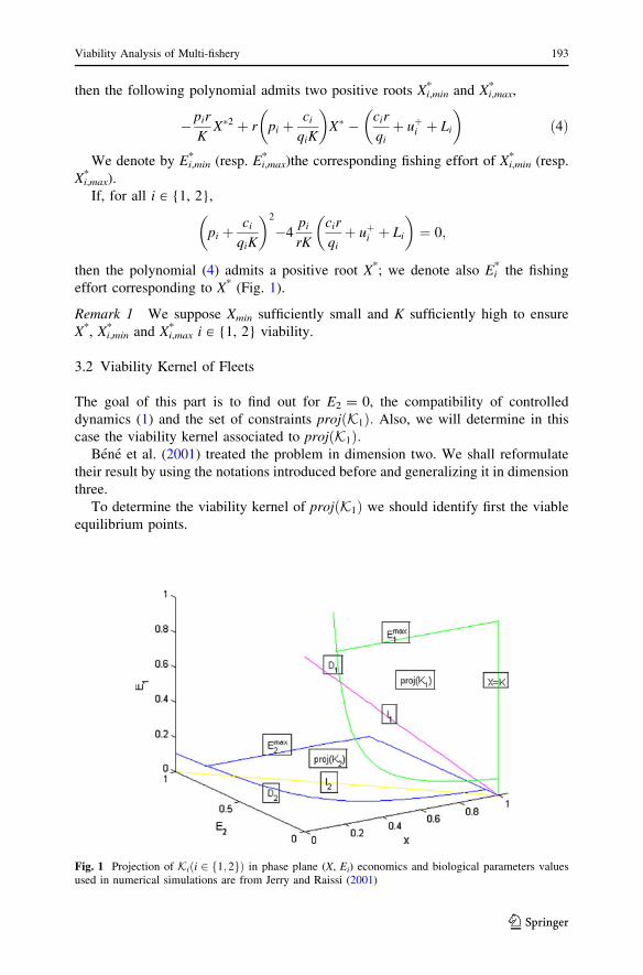
case the viability kernel associated to projðK1Þ:Bene et al. (2001) treated the problem in dimension two. We shall reformulate

their result by using the notations introduced before and generalizing it in dimension

three.

To determine the viability kernel of projðK1Þ we should identify first the viable

equilibrium points.

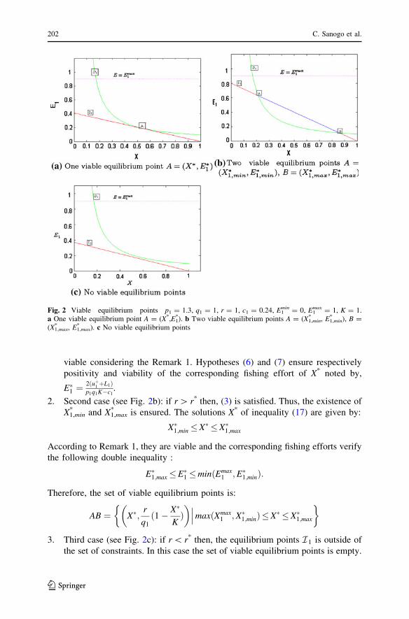
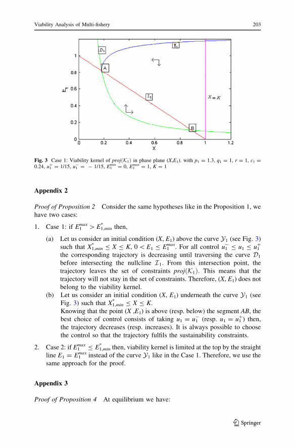
Fig. 1 Projection of Kiði 2 f1; 2gÞ in phase plane (X, Ei) economics and biological parameters valuesused in numerical simulations are from Jerry and Raissi (2001)


123

3.2.1 Viable Equilibrium Points in the Phase Plane (X, E1)

The projection of (1) in phase plane (X, E1) is given by:

_X ¼ FðXÞ � q1E1X_E1 ¼ u1ðtÞ

Xð0Þ ¼ X0; E1ð0Þ ¼ E01:

8<

:ð5Þ

Existence of viable equilibrium points corresponding to (5) are obtained by the

following proposition. Proof of this proposition is left in the ‘‘Appendix 1’’

Proposition 1 Under following conditions:

K [ maxc1

p1q1

;c2

p2q2

� �

ð6Þ

Emaxi � 2ðuþi þ LiÞ

piqiK � ci; i 2 f1; 2g ð7Þ

r� r� ¼ 4p1q21Kðuþ1 þ L1Þ

ðc1 � p1q1KÞ2ð8Þ

Emax1 �E�1;max ð9Þ

and if (3) is fulfilled, then the set of viable equilibrium points correspondingto (5) is given by the segment AB, where

AB ¼ X�;r

q1

1� X�

K

� ��

maxðXmax1 ;X�1;minÞ�X� �X�1;max

��

� �

and Xmax1 ¼ K 1� q1Emax

1

r

� �is the biomass level when E1 = E1

max.

Remark 2 The condition (6) is equivalent to K piqi [ ci, with i [ {1,2} this is a

condition of fishing activity viability, it indicates that the fleet participates in fishing

activity only if the minimum income is ensured.

The condition (7) indicates that at equilibrium the fishing effort must not exceed

the limit capacity imposed. Otherwise, the fleet is forced to leave fishery.

The conditions (8) and (9) play important roles in the determination of viability

kernel. The first one gives us a minimal intrinsic growth rate r* below which the activity

of fishing is not viable the second reveals to us a minimum threshold of effort E1,max* .

3.2.2 Calculation of Kernel Viability of projðK1Þ

In this paragraph we have to characterize the viability kernel of projðK1Þ noted by

ViabðprojðK1ÞÞ and defined by,

ViabðprojðK1ÞÞ ¼ ðX;E1Þ9u1ð:Þwith u�1 � u1ðtÞ� uþ1 such that the solution

ðXð:Þ;E1ð:ÞÞ of ð5Þ starting at ðX;E1Þ stays in projðK1Þ

��

� �


123

Proposition 2 Under the same hypotheses in (1) one of the two following casesoccurs:

1. Case 1: if E1max [ E1,min

* , then

ViabðprojðK1ÞÞ ¼ ðX;E1ÞX�1;min�X�K; and ðX;E1Þ

is between the curvesD1 and Y1

��

� �

where Y1 ¼ ðXð:Þ;E1ð:ÞÞis solution of the following Cauchy problem,

_X ¼ �FðXÞ þ q1E1X_E1 ¼ �u�1

X0 ¼ X�1;min; E0 ¼ E�1;min:

8<

:

2. Case 2: if E1max B E1,min

* , then,

ViabðprojðK1ÞÞ ¼ ðX;E1ÞXmax

1 �X�K; if E1�Emax1 and

ðX;E1Þ is above curveD1

��

� �

Proof See ‘‘Appendix 2’’. h

Remark 3 The curve Y1 defines the upper boundary of the viability kernel,

Y1represents the states of the system where it is necessary to change the control and

thus fishing effort in order to prevent the system from leaving the set of the

constraints.

We have made the same work with the fleet 2 by considering that E1 = 0, in the

same way we obtain the following results:

Proposition 3 Under hypotheses (3), (6) and (7) and under the followingconditions:

r� r0� ¼ 4p2q22Kðuþ2 þ L2Þ

ðc2 � p2q2KÞ2

Emax2 �E�2;max

the set of viable equilibrium points is given by:

A0B0 ¼ X�;r

q2

1� X�

K

� ��

maxðX0max;X�2;minÞ�X�X�2;max

��

� �

and the viability kernel ViabðprojðK2ÞÞ is given by:


* then,

ViabðprojðK2ÞÞ ¼ ðX;E2ÞX�2;min�X�K; and ðX;E2Þ

is between the curvesY2 andD2

��

� �

where Y2 ¼ ðXð:Þ;E2ð:ÞÞ is solution following Cauchy problem,


123

_X ¼ �FðXÞ þ q2E2X_E2 ¼ �u�2

E0 ¼ E�2;min; X0 ¼ X�2;min

8<

:


* then

ViabðprojðK2ÞÞ ¼ ðX;E2ÞX�2;min�X�K; if 0\E2�Emax

2 andðX;E2Þ is above curve D2:

��

� �

3.2.3 Viable Equilibrium Points in Space (X, E1, E2)

After having determined the viability kernel of constraint sets K1 and K2 in the

phase planes (X, E1) and (X, E2), it remains to find out the viability kernel

corresponding to each set of constraints in space (X, E1, E2).

In the space (X, E1, E2) the goal is to determine the compatibility of controlled

dynamics (1) and the set of constraints K1: Also, we will determine the viability

kernel of K1: First, we should identify the viable equilibrium points.

To avoid the exclusion of one of the two fleets, it is necessary to compel the

fishing efforts to remain upper a positive quantity and lower than a limited capacity.

For fleet 2 this limit is given by:

E��2 ¼r

q2

1� c1

p1q1K

� �

�

ffiffiffiffiffiffiffiffiffiffiffiffiffiffiffiffiffiffiffiffi

ðuþ1 þ L1Þrp1K

s !

:

As in Sect. 3.1, the identification of viable equilibrium points is a fundamental

stage in the determination of the viability kernel. It involves the determination of the

set of equilibrium points in the space (X, E1, E2):

P ¼ X;1

q1

r 1� X

K

� �

� q2E2

� �

;E2

� �

=Xmin\X�K; 0�E2�Emax2

� �

:

In Sect. 3.1, for E2 = 0 we had the curve D1: In this section for E2 varying from a

minimal value to a maximal one we have a surface defined by:

D1;s ¼ X;ðuþ1 þ L1Þðp1q1X � c1Þ

;E2

� �

=X��1;min�X�K; 0�E2�E��2

� �

:

Below surface D1;s the minimal income Li, i [ {1, 2}, is not guaranteed for

fleets.

Still in the setting of geometric considerations let us define the surfaces Ks and

E1,smax which delimit the set of constraints K1:

Ks ¼ ðK;E1;E2Þ= 0�E1�Emax1 ; 0�E2�Emax

2

�;

Emax1;s :¼ ðX;Emax

1 ;E2Þ=X��1;min�X�K; 0�E2�E��2

n o:

If


123

p1ðr � q2E�2Þ þc1r

q1K

� �2

[ 4p1r

K

c1

q1

ðr � q2E�2Þ þ ðuþ1 þ L1Þ� �

; ð10Þ

then the following polynomial

� p1r

KX�2 þ p1ðr � q2E�2Þ þ

c1r

q1K

� �

X� � c1

q1


ð11Þ

two positive roots:

X��1;min ¼K

2rp1


q1K

� �

�ffiffiffiffiDp� �

and

X��1;max ¼K

2rp1


q1K

� �

þffiffiffiffiDp� �

with,

D ¼ p1ðr � q2E�2Þ þc1r

q1K

� �2

�4p1r

K

c1

q1


:

We denote by,

E��1;min ¼1

q1

ð1� q2E�2Þ �1

2p1q1


q1K

� �

�ffiffiffiffiDp� �

resp:E��1;max ¼ 1q1ð1� q2E�2Þ � 1

2p1q1p1ðr� q2E�2Þ þ c1r

q1K

� �þ

ffiffiffiffiDp� ��

the corre-

sponding fishing effort of X1,min** (resp. X1,max

** ).

If,


q1K

� �2

¼ 4p1r

K

c1

q1


then the polynomial 11 admits a positive root:

X�� ¼ K

2

c1

p1q1Kþ

ffiffiffiffiffiffiffiffiffiffiffiffiffiffiffiffi

uþ1 þ L1

rp1K

s !

þ c1

2p1q1

:

We also denote by E��1 ¼ r2q1

ffiffiffiffiffiffiffiffiffiffiffiffiffiðuþ

1þL1Þ

rp1K

q

the corresponding fishing effort of X**.

Remark 4 As in dimension two, we suppose that Xmin sufficiently small and

K sufficiently high such that,

Xmin�X��1;min�K and Xmin�X��1;max�K:

The set of viable equilibrium points for fleet 1 is given by the following

proposition, the proof is left in the ‘‘Appendix 3’’:


123

Proposition 4 Under hypothesis (10) and if

1 [1

2

ffiffiffiffiffiffiffiffiffiffiffiffiffiffiffiffiffiffiffi

ðuþi þ LiÞrpiK

s

; ði 2 f1; 2gÞ ð12Þ

E2�E��2 ; ð13ÞEmax

1 �E��1;max: ð14Þ

then the set of viable equilibrium points is given by:

ABC ¼ X�;1

q1

rð1� X�

KÞ � q2E�2

� �

;E�2

� �maxðXmax

1 ;X��1;minÞ�X� �X��1;max;0�E�2 �E��2

��

� �

where Xmax1 ¼ K 1� 1

r ðq1Emax1 þ q2E��2 Þ

� :

Remark 5 As in dimension 2, the condition (12) indicates that no fleet exploits the

fishery if the minimum income is not ensured and (14) reveal that E1,max** is the

minimal threshold of effort for the fleet 1 (Fig. 4).

3.2.4 The Viability Kernel of K1

Let us define the viability kernel of K1:

ViabðK1Þ ¼ ðX;E1;E2Þ9uið:Þwith u�i � uiðtÞ� uþi i 2 f1; 2g so that

the solution ðXð:Þ;E1ð:Þ;E2ð:ÞÞ of :ð1Þstarting at ðX;E1;E2Þ stay inK1

��

8<

:

9=

;

ViabðK1Þ is given by the following proposition which proof is left in the ‘‘Appendix

4’’

Proposition 5 Under hypothesis (10) and conditions (12), (13) and (14), one ofthe following cases occurs:


** then,

ViabðK1Þ ¼ ðX;E1;E2ÞX��1;min�X�K; and ðX;E1;E2Þ isbetween the surfacesD1;s andY1;s

��

� �

where Y1;s ¼ ðXð:Þ;E1ð:Þ;E2ð:ÞÞ is solution of the following Cauchy problem :

_X ¼ �FðXÞ þ q1E1X þ q2E2X;_E1 ¼ �u�1 ;_E2 ¼ �u�2 ;

X0 ¼ X��1;min; E0;1 ¼ E��1;min for all 0�E0;2�E��2 :

8>><

>>:

ð15Þ


** then,

ViabðK1Þ ¼ ðX;E1;E2ÞXmax

1 �X�K; and ðX;E1;E2Þ isbetween the surfacesD1;s andEmax

1;s :

��

� �


123

In the same way as previously, we determine the viability kernel associated to

fleet 2 given by the following proposition (Fig. 5),

Proposition 6 Under hypotheses (10), (12) and following conditions:

E1�E��1Emax

2 �E��2;max:

�

ð16Þ

The set of viable equilibrium points is given by:

A0B0C0 ¼ X�;E�1;1

q2

r 1� X�

K

� �

� q2E�1

� �� maxðXmax

2 ;X��2;minÞ�X�X��2;max;0�E1�E��1

��

� �

where Xmax2 ¼ K 1� 1

r ðq1E��1 þ q2Emax2 Þ

� :

For fixed E1, the set ViabðK2Þ is given by one of two following cases:


** then,

ViabðK2Þ ¼ ðX;E1;E2ÞX��2;min�X�K; and ðX;E1;E2Þ is

between surfacesD2;s and Y2;s

��

� �

where Y2;s ¼ ðXð:Þ;E1ð:Þ;E2ð:ÞÞ is solution of the following Cauchy problem,

_X ¼ �FðXÞ þ q1E1X þ q2E2X;_E1 ¼ �u�1 ;_E2 ¼ �u�2 ;

Xð0Þ ¼ X0;E1ð0Þ ¼ E0;1;E2ð0Þ ¼ E0;2;

8>><

>>:

with, X0 ¼ X��2;min;E0;2 ¼ E��2;min; 0�E01�E��1 :


** then,

ViabðK2Þ ¼ ðX;E1;E2ÞXmax

2 �X�K; and ðX;E1;E2Þ isbetween surfacesD2;s and Emax

2;s

��

� �

with,

D2;s ¼ X;E1;ðuþ2 þ L2Þðp2q2X � c2Þ

� �

=X��2;min�X�K; 0�E1�E��1

� �

;

Emax2;s ¼ ðX;E1;E

max2 Þ=X��2;min�X�K; 0�E1�E��1

n o:

4 Intersection of the Two Viability Kernels K1 and K2

In this section, we determine the intersection of the viability kernels K1 and K2; in

which the two fleets can exploit the resource simultaneously without violating the

constraints. It is convenient to give the following definitions:

– E1,s** = {(X, E1

**, E2)/ X2,min** B X B K, 0 B E2 B E2

max}


123

– E2,s** = {(X, E1, E2

**)/ X1,min** B X B K, 0 B E1 B E1

max}.

The intersection of ViabðK1Þ with ViabðK2Þ is given by the following

proposition, the proof is left in the ‘‘Appendix 5’’:

Proposition 7 Under hypotheses (10), (12) and under conditions (13),(14)

and (16) the viability kernel is given according to the following cases:

1. Case 1: if E2** [ E2,min

** and E1** [ E1,min

**

ViabðK1Þ \ ViabðK2Þ ¼ ðX;E1;E2ÞmaxðX��1;min;X

��2;minÞ�X�K; ðX;E1;E2Þ

is above surfaces D1;s; D2;s

and bellow surfacesY1;s; Y2;s

��

8<

:

9=

;

2. Case 2: if E1** [ E1,min

** and E2** B E2,min

** ,



is above surfacesD1;s;D2;s

and below surfacesY1;s; E��2;s

��

8<

:

9=

;

3. Case 3: if E��1 �E��1;min andE��2 [ E��2;min;



is above surfacesD1;sD2;s

and below surfaces E��1;s; Y2;s

��

8<

:

9=

;

4. Case 4: if E1** B E1,min


** ,



is above surfacesD1;sD2;s

and below surfaces E��1;s; E��2;s

��

8<

:

9=

;

5 Conclusion and Discussion

In this work, we were looking for the management of sustainable exploitation of

renewable resources. Usually, one is inclined towards looking for the optimization

of the net income generated by the exploitation and/or stabilizing the production.

Such objectives allow to elaborate optimal strategies of exploitation. Nevertheless,

directives inspired by such studies are rarely directly applied in practice, especially

in the fishermen community. Asking fishermen to follow a precise strategy for

reaching desired objectives without taking into account external environment is of

course unrealistic.

In this work, we revisited in a new structure based on the concept of viability the

classical bioeconomic models elaborated by Clark (1990). The dynamics is

controlled by the variation of the fishing effort rather than the fishing effort and is

submitted to the constraints that ensure the system viability.


123

The main goal of this study is not to maximize the income generated by the

exploitation, but to analyze the compatibility between the constraints and the

controlled dynamics. We used the viability analysis to build domain of viability

which is the set of initial conditions (efforts, stock) from which the system evolves

without violating the constraints. The viability kernel allows both of the fleets to

exploit the resource simultaneously and guarantees a minimum profit while

maintaining the stock above a minimal level of biomass. In particular for fishery

model, it goes through the introduction of effort and biomass minimal thresholds

and thus aims at reconciling ecological and economical objectives.

Indeed, the use of viability theory permitted us to find out a viability domain in

which the conservation of the resource and the exploitation activity are ensured. In

other terms it allowed us to characterize satisfactory management policies. Several

fleets with different characteristics can exploit the resources simultaneously and of

them will generate at least a minimal income.

These results are obtained in the setting where the natural growth rate of the

resource is represented by a logistic law. It is clear that in this study the model is built

on simplistic hypotheses. However, we showed that Li;E��i ; ði 2 f1; 2gÞ;and r* play

together a crucial role in the vacuity of viability kernel. In further we aim to include the

fact that the fishing efforts vary according to the investment. We hope to incorporate

the dynamics of price and the demand in order to make the model more realistic.

Generally, we believe that the viability approach may provide an interesting

analytical framework to address some of the issues experienced in natural resource

management and sustainable development.

Acknowledgements We would like to thank the two anonymous referees for their helpful comments.

Appendix 1

Proof of Proposition 1 The equilibrium points of (5) are X = 0 and

X� ¼ K 1� q1E�1r

� �

:

It is easy to see that X = 0 is not viable. The equilibrium points (X*, E1*) Must verify

the constraints r1, r2 and r3.

The expression of constraint r2 compared to X* is

ðp1q1X� � c1ÞE�1 � uþ1 � L1

which can be written according to X* as follows

� p1r

KX�2 þ r p1 þ

c1

q1K

� �

X� � c1r

q1

þ uþ1 þ L1

� �

� 0: ð17Þ

The resolution of this inequality depends on the position of r with respect to r*:

1. First case (see Fig. 2a): if r = r*, then (3) is satisfied and the inequality (17) is

reduced in a quadratic equation admitting a double root X� ¼ K2þ c1

2p1q1which is


123

viable considering the Remark 1. Hypotheses (6) and (7) ensure respectively

positivity and viability of the corresponding fishing effort of X* noted by,

E�1 ¼2ðuþ

1þL1Þ

p1q1K�c1.

2. Second case (see Fig. 2b): if r [ r* then, (3) is satisfied. Thus, the existence of

X1,min* and X1,max

* is ensured. The solutions X* of inequality (17) are given by:

X�1;min�X� �X�1;max

According to Remark 1, they are viable and the corresponding fishing efforts verify

the following double inequality :

E�1;max�E�1 �minðEmax1 ;E�1;minÞ:

Therefore, the set of viable equilibrium points is:

AB ¼ X�;r

q1

ð1� X�

KÞ

� �

maxðXmax1 ;X�1;minÞ�X� �X�1;max

��

� �

3. Third case (see Fig. 2c): if r \ r* then, the equilibrium points I1 is outside of

the set of constraints. In this case the set of viable equilibrium points is empty.

Fig. 2 Viable equilibrium points p1 = 1.3, q1 = 1, r = 1, c1 = 0.24, E1min = 0, E1

max = 1, K = 1.a One viable equilibrium point A = (X*,E1

*). b Two viable equilibrium points A = (X1,min* , E1,min

* ), B =(X1,max

* , E1,max* ). c No viable equilibrium points


123

Appendix 2

Proof of Proposition 2 Consider the same hypotheses like in the Proposition 1, we

have two cases:


* then,

(a) Let us consider an initial condition (X, E1) above the curve Y1 (see Fig. 3)

such that X1,min* B X B K, 0 \ E1 B E1

max. For all control u1- B u1 B u1

?

the corresponding trajectory is decreasing until traversing the curve D1

before intersecting the nullcline I1: From this intersection point, the

trajectory leaves the set of constraints projðK1Þ: This means that the

trajectory will not stay in the set of constraints. Therefore, (X, E1) does not

belong to the viability kernel.

(b) Let us consider an initial condition (X, E1) underneath the curve Y1 (see

Fig. 3) such that X1,min* B X B K.

Knowing that the point (X ,E1) is above (resp. below) the segment AB, the

best choice of control consists of taking u1 = u1- (resp. u1 = u1

?) then,

the trajectory decreases (resp. increases). It is always possible to choose

the control so that the trajectory fulfils the sustainability constraints.


* then, viability kernel is limited at the top by the straight

line E1 = E1max instead of the curve Y1 like in the Case 1. Therefore, we use the

same approach for the proof.

Appendix 3

Proof of Proposition 4 At equilibrium we have:

Fig. 3 Case 1: Viability kernel of projðK1Þ in phase plane (X,E1). with p1 = 1.3, q1 = 1, r = 1, c1 =0.24, u1

? = 1/15, u1- = - 1/15, E1

min = 0, E1max = 1, K = 1


123

rX 1� XK

� � q1E1ðtÞXðtÞ � q2E2XðtÞ ¼ 0;

u1 ¼ 0;u2 ¼ 0:

8<

:

It is easy to see that X = 0 is not viable. The other equilibrium points of (1) belong

to the plane whose equation is:

X� ¼ �K

rq1E�1 þ K 1� q2E�2

r

� �

ð18Þ

These equilibrium points (X*, E1*, E2

*) are viable if they verify constraints

r1, r2, r3.

The expression of the constraint r2 is :

� p1rK X�2 þ p1ðr � q2E�2Þ þ c1r

q1K

� �X� � c1

q1ðr � q2E�2Þ þ ðuþ1 þ L1Þ

� �� 0: ð19Þ

For all E2* fixed, the resolution of this inequality depends on the position of E2

*

relatively to E2**.

1. First case : if E2* = E2

** then, hypothesis (10) is satisfied. It implies that the

associated equation (19) admits only one positive root,

X�� ¼ K

2

c1

p1q1Kþ

ffiffiffiffiffiffiffiffiffiffiffiffiffiffiffiffi

uþ1 þ L1

rp1K

s !

þ c1

2p1q1

;

and E��1 ¼ r2q1

ffiffiffiffiffiffiffiffiffiffiffiffiffiðuþ

1þL1Þ

rp1K

q

is the corresponding effort of fleet 1. Therefore, there is only

one stationary point (X**, E1** , E2

**) its viability is ensured by hypothesis (12).

2. second case : if E2* \ E2

** the hypothesis (12) ensures the existence of

X1,min** , X1,max

** as the smallest and the biggest solution of equation (19)

respectively. The other solutions verify the following double inequality :

X��1;min�X� �X��1;max

Fig. 4 Set of viable equilibrium points in space (X, E1, E2) p1 = 1.3, q1 = 1, r = 1, c1 = 0.24,E1

min = 0, E1max = 1, E2

min = 0, E2max = 1, 2, K = 1


123

and are viable according to Remark 3. By using (18) the expression of the fishing

effort of fleet 1 corresponding to X* is:

E�1 ¼1

q1

r 1� X�

K

� �

� q2E�2

� �

:

Therefore, the set of viable stationary points is given by ABC.

3. Third case : if E2* [ E2

** then, the plane Pis underneath surface D1s: Therefore,

no stationary point belongs to the set of constraint. Finally, the set of viable

stationary points is empty.

Appendix 4

Proof of Proposition 5 For all 0 B E2 B E2** we have,


** ,

(a) Let us consider an initial condition (X, E1, E2) above surface Y1;s such that

X1,min* B X B K. For all control u1

- B u1 B u1? the solution of the

dynamical system (1) decreases until traversing surface D1;s before

intersecting the surface P: From this intersection point with the surface

D1;s the trajectory leaves the set of constraints K1: Therefore (X, E1, E2)

does not belong to the viability kernel.

(b) Let us consider an initial condition (X, E1, E2) between surfaces D1;s and

Y1;s such that X1,min** B X B K.

Above the surface ABC one takes u1 = u1- then, for all admissible control

u2 the trajectory solution of dynamical system (1) decreases until

traversing surface ABC. Underneath surface ABC one take u1 = u1? then

the corresponding trajectory increases with respect to X and to E1 until

crossing the surface ABC. Therefore, there always exists a control choice

Fig. 5 Viability kernel of K1 in space (X, E1, E2). p1 = 1.3, q1 = 1, r = 1, c1 = 0.24, u1? =

1/15, u1- = - 1/15, E1

min = 0, E1max = 1, E2

min = 0, E2max = 1, 2, K = 1


123

to ensure that the trajectory fulfils the sustainability constraints. Finally,

(X, E1, E2) belongs to viability kernel.


** then viability kernel is different from the previous case

by the surface E1,smax which delimits it at the top instead of the surface Y1;s:

Therefore, the same argument for the proof of Case 1 is valid in this case.

Appendix 5

Proof of Proposition 7

1. Case 1: if E��2 [ E��2;min and E��1 [ E��1;min

(a) Let us consider an initial condition (X, E1, E2) above surfaces Y1;s and

Y2;s such that max(X1,min** , X2,min

** ) B X B K. For all control u�i � ui� uþi ;ði 2 f1; 2gÞ the solution of dynamical system (1) decreases until traversing

one of the surfaces D1;s or D2;s and leaves one of the sets of constraints K1

or K2 before intersecting surface P: Therefore, (X, E1, E2) does not

belong to viability kernel.

(b) Let us consider an initial condition (X, E1, E2) above surfaces D1;s; D2;s

and underneath surfaces Y1;s; Y2;s; such that max(X1,min** , X2,min

** ) B

X B K. Above surface ABC \ A0B0C0; we take ui ¼ u�i ; ði 2 f1; 2gÞthe solution of dynamical system (1) decreases until crossing surface

ABC \ A0B0C0: Underneath this intersection we take ui ¼ uþi ; ði 2f1; 2gÞ the corresponding trajectory increases until traversing surface

ABC \ A0B0C0: Therefore, there always exists a choice of control that

maintains the trajectory in the constraints domain.

2. Case 2: if E��1 [ E��1;min and E��2 �E��2;min

We notice that the viability kernel is different from the one in Case 1. by

surface E2,s** which delimits it in top instead of Y2;s:

3. Case 3: if E��1 �E��1;min and E��2 [ E��2;min

In this case we find that the viability kernel is different from the one in Case 1.

by surface E1,s** which replaces the limit surface Y1;s:

4. Case 4: if E1** B E1,min


**

The viability kernel is different from the viability kernel of Case 1. this time by

two surfaces E2,s** and E1,s

** . The first (resp. the second) appears instead of Y2;s

(resp. Y1;s). Therefore, we use the same argument in Case 1 for the proofs of

these three last cases.

References

Assessment ME (2005) Ecosystems and human well-being: biodiversity synthesis. http://www.millen

niumassessment.org/proxy/document.354.aspx


123

http://www.millenniumassessment.org/proxy/document.354.aspx

http://www.millenniumassessment.org/proxy/document.354.aspx

Bene C, Doyen L, Gabay D (2001) A viability analysis for a bio-economic model. Ecol Econ

36(3):385–396. ISSN 0921-8009

Clark C (1990) Mathematical bioeconomics: the optimal management of renewable resources. 2nd edn.

Wiley, New York

Doyen L, Pereau J (2009) Sustainable coalitions in the commons. Cahiers du GREThA

FAO (2004) The state of world fisheries and aquaculture. Technical guidelines for Responsible Fisheries

4, Suppl 2, FAO

Jerry M, Raissi N (2001) A policy of fisheries management based on continous fishing effort. J Biol Syst

9(4):247–254. ISSN 0218-3390

Mullon C, Freon P (2006) Prototype of an integrated model of the worldwide system of small pelagic

fisheries. In: Climate change and the economics of the world’s fisheries: examples of small pelagic

stocks. Edward Elgar Publishing, pp 262–295. ISBN 1845424476

Raissi N. (2001) Features of bioeconomics models for the optimal management of a fishery exploited by

two different fleets. Nat Resour Model 14(2): 287–310. ISSN 1939-7445


123

Date post:	26-Aug-2016
Category:	Documents
Upload:	n
View:	214 times
Download:	1 times

Viability Analysis of Multi-fishery

Documents