Page 1
Department of Mechanical and Aerospace Engineering
Viability of river source heat pumps for
district heating
Author: Andrew Lyden
Supervisor: Dr Nicolas Kelly
A thesis submitted in partial fulfilment for the requirement of the degree
Master of Science
Sustainable Engineering: Renewable Energy Systems and the Environment
2015
Page 2
Copyright Declaration
This thesis is the result of the author’s original research. It has been composed by the
author and has not been previously submitted for examination which has led to the
award of a degree.
The copyright of this thesis belongs to the author under the terms of the United
Kingdom Copyright Acts as qualified by University of Strathclyde Regulation 3.50.
Due acknowledgement must always be made of the use of any material contained in,
or derived from, this thesis.
Signed: Andrew Lyden Date: 04/09/2015
Page 3
Abstract
This project aims to investigate the viability of implementing a river source heat pump
which is capable of driving a district heating network. The heat sources most currently
used in the UK are typically the air and the ground. Water is widely available in urban
areas of the UK and is capable of delivering large quantities of heat. Using a heat
pump, this heat has the potential to be used to drive a district heating network.
A generic methodology was developed to aid the investigation. The value in this tool
is its ability to be applied to areas throughout the UK. The methodology covers the
core aspects of technical, environmental and economic. The River Clyde running
through Glasgow was chosen as the case study for the investigation. The suitability of
the river was analysed and a demand/supply matching model was created in an Excel
spreadsheet to consider technical aspects of the heat pump. The method for
identifying potential areas near to the Clyde was applied to choose a suitable location.
Environmental concerns were analysed in terms of impact assessment, CO2 equivalent
emissions and air quality. A financial model was created using a discount cash flow
method, allowing for comparisons between different heating configurations. These
were gas boilers only, gas boilers and conventional electric heating, CHP only and the
river source heat pump and CHP.
The River Clyde was found to be suitable for a large heat delivery, with a proposed
heat pump of 6.65 MW. The method for identification of a district heating site
identified a large part of the Merchant City, which could potentially benefit from
district heating. The demand/supply matching model produced a variety of interesting
technical results, importantly showing that an annual heat demand of 40 GWh is a
good match for the proposed heat pump. Environmentally the hybrid system of river
source heat pump and CHP provided the lowest CO2 emissions in the long term, with
CHP only having the lowest only for the current year, 2015. A move away from gas
heating systems resulted in better air quality, reducing both NOx and CO emissions.
Economically the CHP and river source heat pump provided the lowest payback
period of 9.79 years, when upgrading from gas boilers, and 5.36 years, when
upgrading from a gas and conventional electric hybrid heating system.
Page 4
Acknowledgements
I’d like to thank my supervisor Dr. Nick Kelly for his help with this thesis. I would
also thank all of the staff involved with the running of the course and to all my fellow
students on the course who helped make this a very enjoyable year.
Thank you to my family and friends for their continued support.
Page 5
Table of Contents 1. Introduction ...................................................................................................... 1
1.1. Aim .................................................................................................................. 2
1.2. Objectives ........................................................................................................ 2
1.3. Overview ......................................................................................................... 3
2. Heat Pumps ....................................................................................................... 4
2.1. Thermodynamics ............................................................................................. 5
2.2. Performance .................................................................................................... 7
2.3. Types of heat pump ......................................................................................... 9
Open-loop systems ............................................................................. 11 2.3.1.
Closed-loop systems ........................................................................... 12 2.3.2.
2.4. Refrigerant fluids ........................................................................................... 13
2.5. Hybrid systems .............................................................................................. 16
2.6. Applications .................................................................................................. 17
2.7. Case study: Shettleston Mine-water Heat Pump ........................................... 18
3. District Heating .............................................................................................. 20
3.1. Principles ....................................................................................................... 21
3.2. Methods of heating ........................................................................................ 21
3.3. Distribution systems ...................................................................................... 22
3.4. Case study: Drammen, Norway .................................................................... 23
4. Methodology ................................................................................................... 25
4.1. River properties ............................................................................................. 25
Flow rate ............................................................................................. 25 4.1.1.
Water temperature .............................................................................. 27 4.1.2.
4.2. River source heat pump ................................................................................. 30
Heat pump sizing ................................................................................ 30 4.2.1.
Case studies: Large-scale water source heat pumps ........................... 33 4.2.2.
COP seasonal variation model ........................................................... 36 4.2.3.
4.3. District heating .............................................................................................. 38
Heat map site identification ................................................................ 38 4.3.1.
Demand profile ................................................................................... 42 4.3.2.
4.4. Demand/Supply matching ............................................................................. 46
Heating system configuration ............................................................. 46 4.4.1.
Technical outcomes ............................................................................ 47 4.4.2.
Page 6
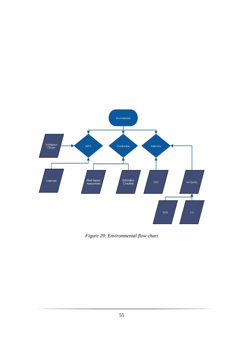
4.5. Environmental ............................................................................................... 49
SEPA regulations ............................................................................... 49 4.5.1.
Construction ....................................................................................... 51 4.5.2.
Emissions and air quality ................................................................... 52 4.5.3.
4.6. Economic ....................................................................................................... 56
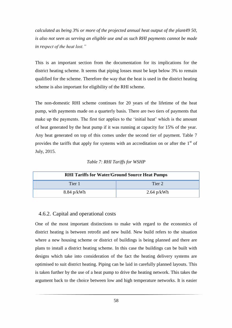
Renewable Heat Incentive (RHI) ....................................................... 56 4.6.1.
Capital and operational costs .............................................................. 58 4.6.2.
Financial model .................................................................................. 61 4.6.3.
5. Results & Analysis ......................................................................................... 65
5.1. River Clyde suitability .................................................................................. 65
5.2. Heat pump size .............................................................................................. 67
5.3. District heating site ........................................................................................ 68
5.4. Demand/Supply matching ............................................................................. 72
5.5. Environmental impact ................................................................................... 77
5.6. Economic comparisons ................................................................................. 82
6. Conclusions ..................................................................................................... 87
6.1. Methodology ................................................................................................. 87
6.2. Results & Analysis ........................................................................................ 89
6.3. Further research ............................................................................................. 92
7. References ....................................................................................................... 93
Page 7
List of figures
Figure 1: Heat pump schematic (Tuohy, 2008) ............................................................. 5
Figure 2: Simple vapour-compression component cycle, T-S diagram for cycle
(Tuohy, 2008), (Moran, 2015) ....................................................................................... 5
Figure 3: Realistic vapour-compression cycle, with heat exchanger (Tuohy, 2008) ..... 6
Figure 4: Relationship between COP and outlet temperature (Mathissen, 2011).......... 8
Figure 5: Closed-loop water source heat pump graphic (KensaHeatPumps, 2015) .... 12
Figure 6: Comparison of refrigerants (IndustrialHeatPumps, 2012) ........................... 14
Figure 7: Monthly variations of gas and electricity demands (Harrison, 2011) .......... 16
Figure 8: Simple schematic of district heating (SmartHeat, 2012) .............................. 20
Figure 9: Drammen typical day heating demand profile (Hoffman, 2011) ................. 24
Figure 10: River flow rate, River Don ......................................................................... 26
Figure 11: Flow rate exceedance curve, River Don ..................................................... 27
Figure 12: Example river temperature plot .................................................................. 28
Figure 13: River properties flow diagram .................................................................... 29
Figure 14: Duindorp, with heat pump arrangement (Stoelinga, 2009) ........................ 33
Figure 15: Kingston Heights heat pump system (Smith, 2014) ................................... 34
Figure 16: Largest water heat pump in the world, Värtan Ropsten (Nowacki, 2014) . 35
Figure 17: Seasonal variation of COP, River Clyde .................................................... 36
Figure 18: River source heat pump flow diagram ....................................................... 37
Figure 19: Heat Map Scotland: Overview of Scotland ................................................ 39
Figure 20: Glasgow heating demand map ................................................................... 40
Figure 21: Heat map, low-carbon technologies, yellow: ASHP, green: Biomass ....... 41
Figure 22: Heat map, social housing and district heating icons .................................. 41
Figure 23: Residential thermal demand profile ........................................................... 43
Figure 24: Commercial thermal demand profile .......................................................... 43
Figure 25: Office thermal demand profile ................................................................... 44
Figure 26: District heating flow diagram ..................................................................... 45
Figure 27: CAR authorisation process ......................................................................... 50
Figure 28: Glasgow, example annotated piping network ............................................ 51
Figure 29: Environmental flow chart ........................................................................... 55
Figure 30: Economic flow chart .................................................................................. 64
Page 8
Figure 31: Flow exceedance curve for the River Clyde .............................................. 66
Figure 32: Monthly temperature data, Clyde Sea (ScottishGovernment, 2012) .......... 67
Figure 33: Central Glasgow heating demands ............................................................. 68
Figure 34: Proposed area for district heating ............................................................... 69
Figure 35: Social housing percentage for proposed area ............................................. 70
Figure 36: Thermal demand profile of proposed site ................................................... 71
Figure 37: Electricity consumption vs. Annual demand .............................................. 72
Figure 38: Percentage of capacity of WSHP used vs. Annual demand ....................... 73
Figure 39: Capacity of CHP required vs. Annual demand .......................................... 74
Figure 40: Percentage of demand provided by WSHP vs Annual demand ................. 75
Figure 41: Distribution systems vs. Annual Demand .................................................. 76
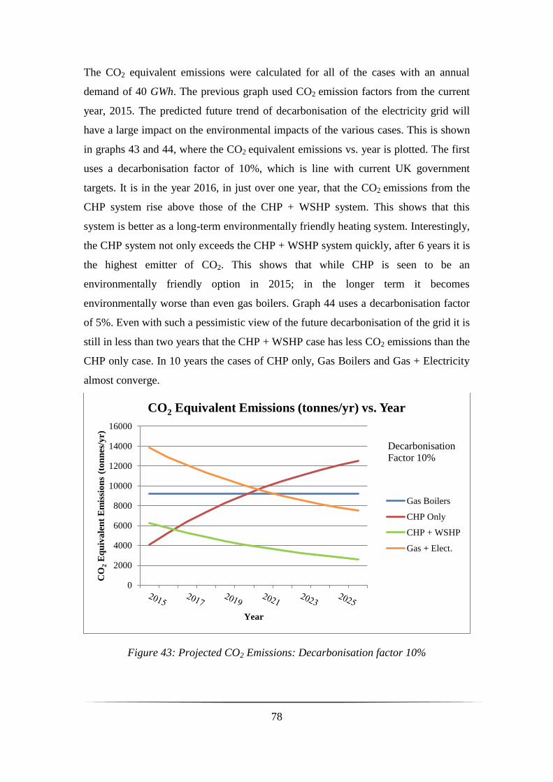
Figure 42: Comparison of cases: CO2 emissions vs. Annual demand ......................... 77
Figure 43: Projected CO2 Emissions: Decarbonisation factor 10%............................. 78
Figure 44: Projected CO2 Emissions: Decarbonisation factor 5%............................... 79
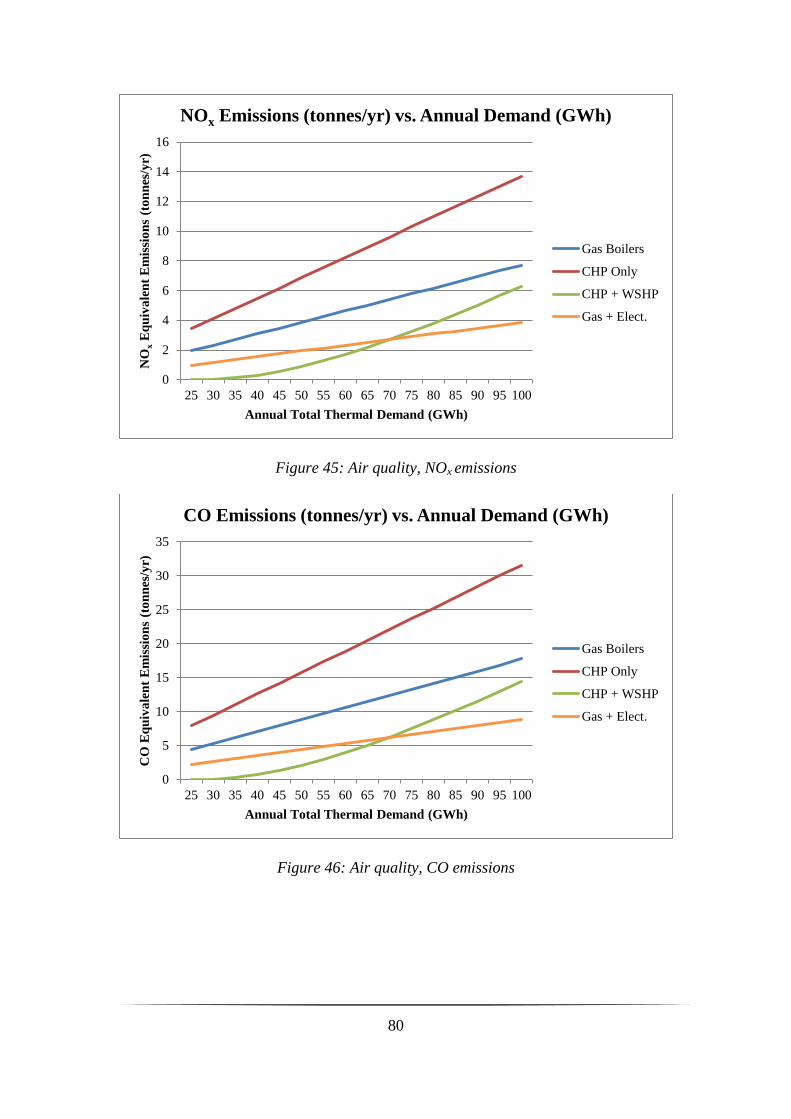
Figure 45: Air quality, NOx emissions ......................................................................... 80
Figure 46: Air quality, CO emissions .......................................................................... 80
Figure 47: CO2 emissions: Distribution systems ......................................................... 81
Figure 48: With and without RHI payments comparison ............................................ 82
Figure 49: Annual savings of cases vs. Annual demand ............................................. 83
Figure 50: Distribution systems: Annual cost vs. Annual demand .............................. 84
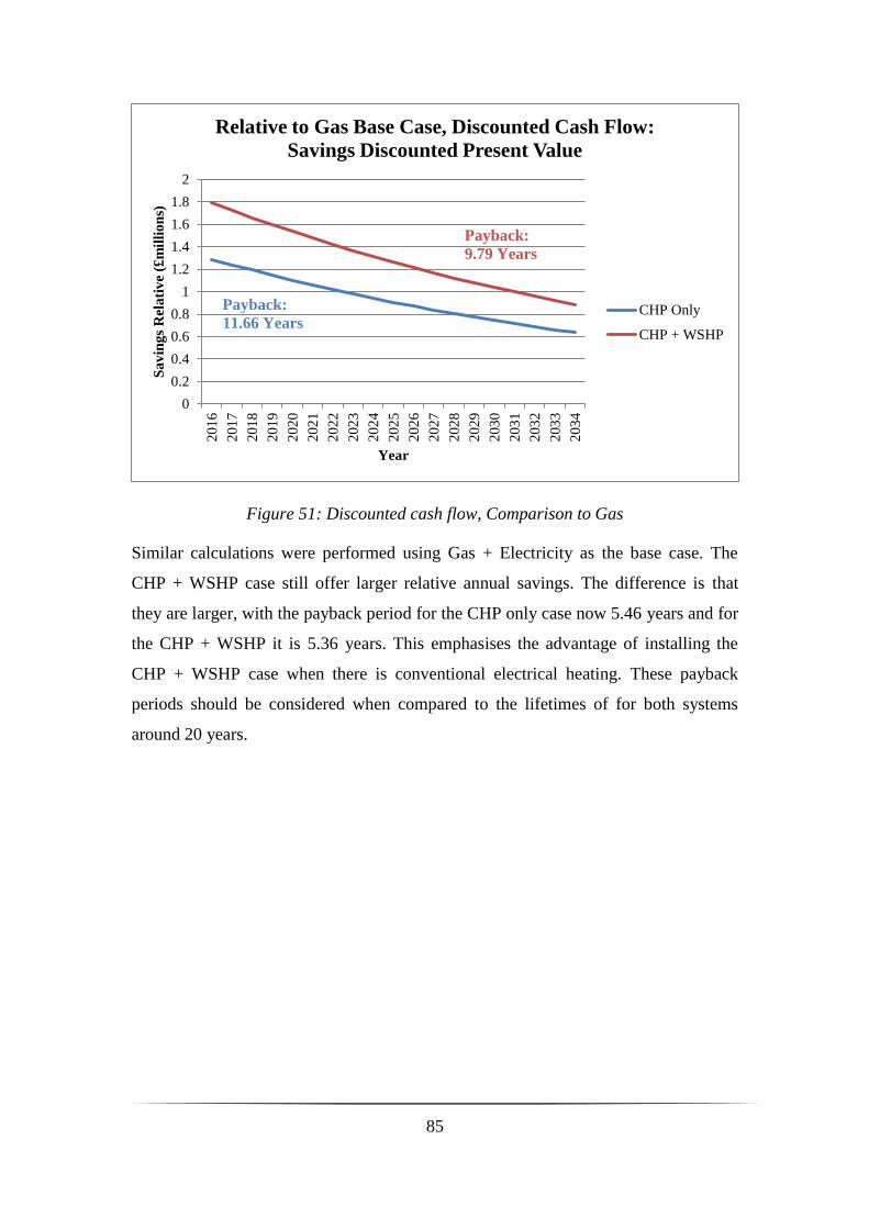
Figure 51: Discounted cash flow, Comparison to Gas ................................................ 85
Figure 52: Discounted cash flow, Comparison to Gas + Elec. .................................... 86
Page 9
List of tables
Table 1: Comparison of GSHP and ASHP. Help from (Wu, 2009) ............................ 10
Table 2: Thermal demand characteristics of building class ......................................... 42
Table 3: Heating system configurations of the four cases ........................................... 47
Table 4: Environmental checklist for piping ............................................................... 52
Table 5: CO2 equivalent emission factors for gas ........................................................ 53
Table 6: NOX and SOX emission factors for gas (USEPA, 1995) ............................. 54
Table 7: RHI Tariffs for WSHP ................................................................................... 58
Table 8: Heat pump: Capital costs ............................................................................... 59
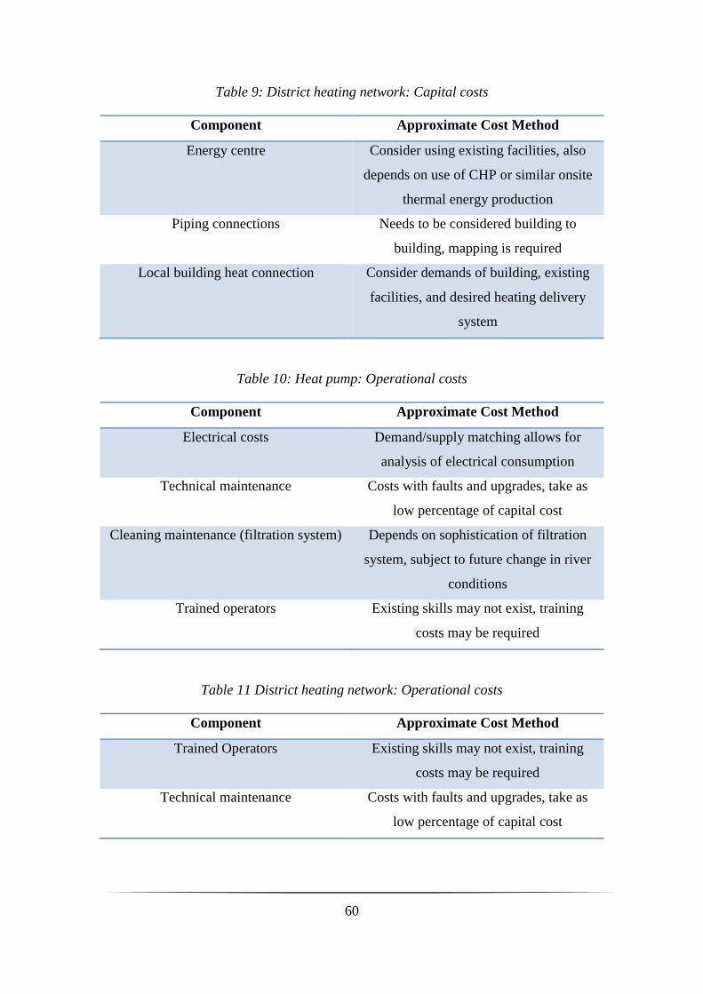
Table 9: District heating network: Capital costs .......................................................... 60
Table 10: Heat pump: Operational costs ...................................................................... 60
Table 11 District heating network: Operational costs.................................................. 60
Table 12: Estimations for costs .................................................................................... 61
Table 13: Gas and electricity prices ............................................................................. 61
Page 10
1
1. Introduction
Heating currently makes up a large proportion of the energy use worldwide,
particularly in countries with milder climates such as the UK. Recently there has been
a concentrated effort at increasing the sustainability of the net energy used. This has
seen great advances in the installation of large capacities of wind farms and solar
power as well as the development of ever maturing technologies such as tidal and
wave power devices. This has led to a trend of decarbonisation of the electricity grid,
which should continue due to direct governmental intervention, rising fossil fuel costs
and cheaper available renewable energy. Despite this, there has not been the same
drive towards sustainability in the heating sector.
There have been improvements in energy efficiency standards for buildings, with ever
tightening government legislation causing great reductions in energy use for newly
constructed buildings. Legislation does however lag for the current building stock so
that improvements can still be made in this area, particularly with projections
predicting 85% of the current housing stock in the UK will remain by 2050 (Kannan
& Strachan, 2009). Even if standards for energy efficient buildings improve there will
still be a vast requirement for heating.
Currently the heating demand of the UK is met primarily by gas, supplemented by
electricity and oil. Heat pumps have the potential to provide a low-carbon solution for
the provision of heat. The sources of heat for heat pumps are low grade and are
widely available in urban areas. Currently the greatest uptake of this technology has
been with ground and air sourced heat pumps. These utilise the solar heat absorbed by
both the earth and the atmosphere. The heat pump provides a way of promoting this
low-grade heat up to useful temperatures capable of providing space heating and
direct water heating.
Water sourced heat pumps transfer the vast heat available from the abundant sources
of water which intertwine with the cities and towns of the UK. From coastal towns on
Page 11
2
the sea, to inland towns built up alongside lakes, to ex-mining towns sitting above
now-abandoned mine shafts, some of which have filled with temperate groundwater,
to aquifers underground scattered all over the UK’s fractured geological crust, to the
fast-flowing rivers so many cities have built up alongside. The potential for heating
from these sources of heating is immense. Instead of having to ship gas hundreds of
miles from distant countries at large carbon expense, heat pumps provide a means of
locally sourcing a low-carbon, sustainable source of heating.
1.1. Aim
Glasgow sandwiches the River Clyde as well as many other smaller rivers such as the
River Kelvin. The Clyde splits the city through dense urban and industrial sites, many
of which have large heating demands. The aim of this thesis will be to investigate the
aspects involved with implementing a large heat pump using the River Clyde, which
is capable of providing a substantial amount of heat via a district heating network.
The proposed network will draw a large proportion of its heat from the river source
heat pump.
1.2. Objectives
The main objectives of the project are outlined below:
Developing a generic methodology capable of investigating the viability of
river source heat pumps driving a district heating network, addressing
technical, environmental and economic aspects
Building an Excel spreadsheet model capable of performing demand/supply
calculations for river source heat pumps
Investigation into the viability of the River Clyde as a heat source
Analysis of the technical aspects of a river source heat pump on the River
Clyde
Analysis of the various environmental advantages and disadvantages of a river
source heat pump with district heating in Glasgow
Page 12
3
Determining the economic viability of a river source heat pump to provide
district heating to an area of central Glasgow
1.3. Overview
In section 2, Heat Pumps, the thermodynamic background of heat pumps will be
presented along with factors regarding performance. It will discuss various types of
heat pumps and include technical information regarding the impact of the choice of
refrigerant fluid. This is followed by sub-sections on how heat pumps perform with
other heating devices and also where their application is suitable. The section
concludes with a case study on the Shettleston Mine-water Heat Pump.
Section 3 introduces the facets of district heating, explaining the principles and what
heating systems they use. It ends with the case study of a heat pump driven district
heating scheme, Drammen, Norway.
In section 4, Methodology, the generic methodology capable of investigating the
viability of river source heat pumps driving a district heating network is presented. It
considers analysis of the proposed river as well as the technical details of the heat
pump involved. Mapping techniques and technical considerations of district heating
are then discussed. The method for developing the demand/supply matching Excel
spreadsheet is argued, with the following two sub-sections outlining the
environmental and economic considerations which require deliberation.
The Results and Analysis of section 5 applies the methodology outlined to the case of
the River Clyde, Glasgow.
Section 6, Conclusions, brings the various discussions and analysis throughout the
thesis together, including suggestions for further areas of research.
Page 13
4
2. Heat Pumps
Heat can never pass from a colder to a warmer body without some other change,
connected therewith, occurring at the same time.
Clausius statement
According to the Clausius statement of the 2nd
law of thermodynamics it is impossible
for heat to flow from an area of low temperature to an area of high temperature
without the aid of an external force. This is obvious from real life experience as when
a hand touches a hot object, for example boiling water, the person feels a dramatic
(and painful) flow of heat from the higher temperature water to the lower temperature
surface of the hand. It is never the case that the heat flows from the hand to the
boiling water.
This fundamental law does, however, include the possibility for heat to flow from
cold to hot with the aid of an external force. This may seem an odd concept but it is
one used by an essential kitchen appliance. Fridges facilitate the flow of heat from a
cool body, the food inside, to a warmer body, the room of the kitchen. This is possible
due to the electrical work performed by the fridge; the electricity acts as the external
force required by the Clausius statement. Essentially the fridge uses electricity to
transfer heat from your butter to warm up your kitchen.
The obvious goal of the fridge is for keeping food cool and the fact that the kitchen
area is heated up in the process is merely a by-product. Using the same
thermodynamic cycle it is possible to provide additional heat to a warmer place from
a cooler place, where this time the cooling of the cool place is the by-product. These
devices are known as heat pumps and also require an external force to operate. Figure
1 below is a simple schematic outlining the thermodynamic processes of a heat pump.
(Cengel, Boles, & Kanoğlu, 2002)
Page 14
5
Figure 1: Heat pump schematic (Tuohy, 2008)
2.1. Thermodynamics
Heat pumps use the same thermodynamic cycle as refrigerators: the vapour-
compression cycle. The simplest form of this cycle uses 4 basic components: a
compressor, an evaporator, an expansion valve and a condenser. The left of figure 2
shows how these connect to form the cycle.
Figure 2: Simple vapour-compression component cycle, T-S diagram for cycle
(Tuohy, 2008), (Moran, 2015)
A fluid passes through the 4 points shown on the left figure. The fluid changes from a
saturated vapour at point 1 to a superheated vapour at point 2 as it goes through the
compressor. Note that it is in the compressor that the electrical work is input. Once
the fluid is a superheated vapour it passes through a condenser which cools the fluid
Page 15
6
to a saturated liquid state at point 3. This is the process by which heat is taken from
the cycle and transferred to the area to be warmed. An expansion valve is then used
between points 3 and 4 to reduce the pressure of the fluid and change the state to
liquid-vapour. Heat is taken into the cycle via the evaporator. Between points 4 and 1
the evaporator uses the heat from a cooler area to change the fluid to a saturated
vapour, and thus ready to enter the compressor to restart the cycle.
The cycle outlined is the ideal one and presumes a perfect, reversible compression
stage. In a real, practical cycle the compression is irreversible meaning the
compressor is required to perform additional work. This can be seen on the P-S
diagram, Figure 3, where the entropy of the practical cycle at point 2 is larger than in
the ideal case, denoted by the point 2s. Another real characteristic of the cycle is
additional sub-cooling of the fluid leaving the condenser as seen by the movement of
point 3 on the same figure. While the evaporator can be exposed to various
conditions, it is necessary for the compressor to work with solely dry vapour making
sub-cooling an essential component. It can be achieved via a heat exchanger between
the fluid leaving the condenser and the evaporator. This more realistic process is
shown in figure 3, along with the P-S diagram.
There are many further considerations to be made with regards to maximising the
performance for a vapour-compression cycle. A flooded or liquid overfeed evaporator
arrangement can improve the heat transfer ability, as opposed to a dry expansion
Figure 3: Realistic vapour-compression cycle, with heat exchanger (Tuohy, 2008)
Page 16
7
evaporator. The work input required by the compressor can also be reduced by using a
multi-stage compression scheme. This introduces a lower, intermediate pressure
which means a reduced pressure ratio across the compressor. This in turn reduces the
work required by the compressor, leading to an increased level of performance.
(Tuohy, 2008)
2.2. Performance
The level of performance for a heat pump is measured by its Coefficient of
Performance (COP). It is defined as the ratio of the useful heating provided to the
electrical input. Note that this is the COP specifically for a heat pump, for a
refrigerator the COP is the ratio of the cooling provided to the electrical input. As
explained earlier, it is simply the desired goal which sets these devices apart. The
previous sub-section ended with a discussion of improvements for the vapour-
compression cycle. The successes of such modifications are explicitly quantified by
whether they increase or decrease the COP of the system. This is an important
measure of the viability of a heat pump system. The UK government is currently
running the Renewable Heat Incentive (RHI), a subsidy for which water source heat
pumps qualify. A requirement to qualify for this is a COP of 2.9, conveying the
importance set against COP. (OFGEM, 2015b)
However, one of the most fundamental factors affecting the COP is the temperature
difference between the environments where heat is being transferred from and where
the heat is going to. For illustration, the COP for a heat pump using the ideal Carnot
cycle can be expressed as
𝐶𝑂𝑃 = 𝑇𝐶𝑜𝑙𝑑
𝑇𝐻𝑜𝑡 − 𝑇𝐶𝑜𝑙𝑑
Where TCold is the temperature of the cold area where heat is being extracted from and
THot is the temperature of the hot area heat is being transferred to. It can be seen that
minimising the difference between the hot area and cold area will result in an
improved COP. (Sonntag, Borgnakke, Van Wylen, & Van Wyk, 1998)
Page 17
8
Another useful measure of the performance of a heat pump can be found by
calculating the Seasonal Performance Factor (SPF). This is defined as the ratio of the
total useful heating provided over a year to the total electrical consumption. This is
useful because the COP of a heat pump is not a temporally static figure. Various
conditions depending on an individual heat pump can affect the day-to-day and
season-to-season COP. The SPF provides a more insightful measure of how a heat
pump is performing under different conditions. (Herold, Radermacher, & Klein, 1996)
An important characteristic for the COP of a heat pump is its variation with respect to
the outlet temperature from the heat pump. Figure 4 illustrates this inverse linear
relationship as well as the reduction of COP in relation to the ambient air temperature
(this is a generic relationship which is relevant for the temperature of any source, i.e.
applicable to water source heat pumps). Note in the graph the term ‘Entering Water
Temperature’ is equivalent to outlet temperature.
Figure 4: Relationship between COP and outlet temperature (Mathissen, 2011)
Page 18
9
This is important because it shows how useful it is to have a heating scheme which
can work with low temperatures so that the heat pump can perform even more
efficiently. (Mathissen, 2011)
2.3. Types of heat pump
The sources of heat for heat pumps are most commonly air, ground and water. Air-
source heat pumps have heat exchangers exposed to the outside environment and
transfer the heat from the air. Ground-source heat pumps consist of heat exchangers
buried in the earth and transfer the heat from there. This thesis concentrates on the
potential of water sourced heat pumps, where the heat exchangers transfer the heat
from a body of water.
In literature water source heat pumps are often referred to as surface water GSHPs
(ground-sourced heat pumps) due to their similarity in function to common GSHPs,
and typically air-sourced heat pumps are abbreviated to ASHP. For clarity this thesis
will refer to water source heat pumps as WSHPs to differentiate them from GSHPs.
The distinct value of a WSHP is in the heat transfer coefficients. Water has a
particularly high convective heat transfer coefficient of 1200 W/m2K, which is for
water flowing in a tube (EngineersEdge, 2015). Compare this to air with a convective
heat transfer coefficient of 100 W/m2K, which is for air travelling at a moderate speed
over a surface (EngineersEdge, 2015), and to the ground conduction heat transfer
coefficient of 1 W/mK, for a moist area (EngineeringToolbox, 2015). Note that air and
water transfer heat by convection, radiation and conduction while the ground does not
transfer heat via the convection process. Water source heat pumps can therefore have
a heat transfer coefficient a factor of up to 10 times larger than those of air or ground
source heat pumps.
Heat transfers more quickly through a wet surface than a dry one. This is why it is
generally desirable to place GSHPs in places with abundant water such to increase
their efficiency. Some of the comparative pros and cons of ground and air source heat
pumps are outlined in table 1.
Page 19
10
WSHPs utilise the low-grade heat of ground water or surface water. Surface water
sources can be rivers, lakes, streams or seawater. Ground water is found beneath the
Earth’s surface in fractured rock spaces (aquifers) or in soil pockets. Reaching
aquifers can require expensive drilling. However, during large construction projects,
in certain geographical areas, these are often exposed. Another possible source is
mine-water. (David Banks, 2012)
GSHP ASHP
Pros Cons Pros Cons
More efficient,
stable temperatures
underground
More upfront cost,
need for drilling
and heat exchanger
underground
More flexible,
system can easily
provide heating in
winter and cooling in
summer
Less efficient,
large seasonal air
temperature
variations
Better visually, out
of sight and silent
Large disruption,
lots of construction
work needed
Easier construction,
no groundwork
necessary
More
maintenance
needs, possibility
of freezing in
winter
Possibility for
using ground as
thermal store
Less upfront cost, no
need for drilling
More visual
impact, visible
and occasional
noise problems
Less maintenance,
heat pump
protected from
elements
underground
More possibility
for vandalism
Table 1: Comparison of GSHP and ASHP. Help from (Wu, 2009)
Page 20
11
Open-loop systems 2.3.1.
Open-loop heat pumps involve the physical abstraction of water from the source and
directly passing it through the heat exchanger where the heat is extracted. When using
a groundwater source, a suitable aquifer is required such that there is a reliable and
usable flux of water so that an extraction well can be built. In reality, to have
sufficient knowledge of the suitability of an underground aquifer requires a specialist
hydrogeologist. The design component of the extraction well requires planning for the
depth of the well as depths of aquifers range from a few metres to 100s of metres, the
diameter of the well which constrains the size of the pump which can be inserted, the
yield of the well which will be dictated by the heat pump size, and the physical
properties of what needs to be drilled which greatly effects the economics. The water
is then either returned to the aquifer or disposed of. For heat pumps utilising surface
water, naturally, there is no need for an extraction well. Water is pumped directly
from the source to the heat exchanger and then returned to source at a lowered
temperature.
These offer high efficiencies as they do not require an intermediate heat transfer
carrier, the heat is transferred directly from the water. The lack of requirement for this
intermediate stage reduces the capital cost of the system and the simplicity of the
system provides a lower risk of damage to the piping. Care must be taken depending
on the conditions of the water that is being pumped into the heat exchanger. A
filtration system may be needed to protect the heat exchanger from damaging debris.
This increases the required maintenance and power consumption. Therefore an added
design consideration in a preliminary feasibility study would be the water cleanliness
quality. There is also additional power consumption arising from the necessary
pumping of the water. Environmentally open-loop systems can have a direct impact,
this is because the water is being physically moved meaning that living creatures can
be drawn into the pump. (David Banks, 2012)
Page 21
12
Closed-loop systems 2.3.2.
The other system which can be used for WSHPs are closed-loop systems. They
consist of big plates or lattices which are submerged in the water. These use an
intermediate heat transfer stage to transfer heat directly from the water source,
requiring no pumping. This involves an intermediate fluid which is commonly an
antifreeze solution, although it can be a variety of chemicals including ammonia and
glycol.
Figure 5: Closed-loop water source heat pump graphic (KensaHeatPumps, 2015)
They are generally installed as either horizontal or vertical loops, and due to this their
environmental interaction is limited to the water being exposed to these loops.
However, the intermediate fluid if leaked can have potentially damaging effects. Their
design is primarily specified by the properties of the body of water they are to be used
in, with the design generally requiring less maintenance than an open-loop system.
They are more susceptible to damage in rivers than open-loop systems as the
submerged components are liable to float away with high flow rates. In rivers which
are used for shipping the plates are exposed to damage from passing boats. (Russo &
Civita, 2009)
Page 22
13
2.4. Refrigerant fluids
Refrigerants are one of the most important parts of a heat pump and the choice of
which one to use has both significant technical and environmental impacts. In the
function of a heat pump it is the refrigerant which takes the energy from the heat
sources and delivers it to the heat exchanger to be used. Common refrigerants used in
heat pumps, and fridges, also have a high possible global warming impact. Making
the right choice of refrigerant is vital in determining the feasibility of any heat pump
system.
The condensation pressure of refrigerants varies with temperature and this variation is
unique for different refrigerants. Some refrigerants will stop working at too very high
temperatures because the pressure becomes excessive, which can cause damage to the
heat pump’s components. Contrastingly low pressure can also cause risks as the
volume which needs to be swept increases which means that larger, more expensive
heat pump components are needed. Figure 6 graphically shows the relationship
between pressure and temperature for an array of refrigerants. When a refrigerant’s
line on the graph stops, this means that it has reached its supercritical stage. Beyond
the pressure and temperature at this point there is a transition from the liquid to the
gaseous state. This means that only some refrigerants will work for large heat pumps
which require high operating temperatures. Different refrigerants will result in
different COP, and the heat pump system must be designed with this in mind to
achieve optimal results.
Page 23
14
Refrigerants are also prone to leaking into the environment from the heat pump. They
each leak with their own characteristics and, importantly, have varying impacts on
global warming. The leakage occurs during the operation of the heat pump while there
is another risk of escaping refrigerant during disposal after the lifetime of the heat
pump. The impact on the climate due to refrigerant leakage is not negligible compared
with the electricity use. It is estimated 25-30% of total impact is due to refrigerant
leakage for a 56 kWe system which assumes 40-50 percent of the refrigerant is
recovered. (Meacock, 2013)
Two widely used working fluids are CFCs and HFCFs, and they historically offer the
potential for the highest operational COP. These are particularly harmful to the
climate and there is ongoing research into the replacement of the use of these. Balance
is needed between optimising the heat pump via the choice of an effective refrigerant
which raises the COP of the system and the negative climatic impacts these
refrigerants have. There are a number of natural refrigerants which can be, and have
been, used in modern heat pump systems.
CO2, perhaps surprisingly, offers a climate friendly alternative to CFCs and HFCFs as
its climatic impact is in the order of thousands of times lower. It is easy to use with
other substances and technology has advanced such that the high pressures necessary
for CO2 to be used in heat pumps is readily available. Heat pumps which use CO2
should be designed carefully to take into account its specific thermodynamic
Figure 6: Comparison of refrigerants (IndustrialHeatPumps, 2012)
Page 24
15
characteristics. If this is done then the COP reduction normally associated with using
non-CFCs or non-HFCFs can be minimised. CO2 offers a real technically suitable
alternative while vastly reducing the climatic impact.
Hydrocarbons have similar properties to HCFCs and therefore offer a potential
alternative. However, often hydrocarbons, such as propane, are highly flammable and
require a secondary loop for safety reasons to be implemented in the heat pump. This
has the unappealing result of reducing the COP by about 20%. Hydrocarbons are
commonly used in domestic refrigeration.
Water as a refrigerant is very desirable in terms of its climatic impact. It is one of the
oldest used chemicals in refrigeration. Technical problems associated with the heat
pump design do arise due to high specific volume at low temperatures. Ammonia is
another abundant substance capable of acting as the working fluid. It is
environmentally friendly and capable of achieving comparable COPs. The main issue
is that ammonia is highly flammable. Therefore there needs to be a lot of safety
precautions taken in order to design a heat pump which will operate safely. Ammonia
is also a toxic substance. (Stoecker, 1998)
The factors of climate impact, system performance and cost need to be weighed up to
ultimately decide which working fluid should be used in the heat pump. This is a part
of what will ultimately result in the final design of a heat pump and should be taken
early on such that the heat pump is optimised to work with a specific refrigerant.
Page 25
16
2.5. Hybrid systems
Heating demands vary seasonally and as such any potential heat pump needs to be
sized appropriately to obtain the highest possible SPF. Figure 7 shows an example
heating demand over a year. This U-shape trend can be found in a wide variety of
demand profiles and is therefore a useful starting point when sizing a base load
provider such as a heat pump. The easiest solution is to size the heat pump to the
minimum heating demand such that the heat pump provides the entire heating
requirement when the heating load is lowest. This solution requires the need for
external provision of heat.
The purpose of this discussion has been to introduce the important notion of heat
pump hybrid systems. To ensure that the peak heating demand is met throughout the
year devices capable of dispatchable heat production is required. It is also possible to
use renewable heating devices which require no fuel. This means that efficient use of
their output is less important.
The common devices capable of delivering dispatchable heat are commonly gas
boilers, biomass boilers, diesel generators and electrical heating. Gas boilers are the
most commonly used as the systems are cheap to install, expertise is widespread and
the fuel is easily obtained through the gas network. Due to the desire to switch to
Figure 7: Monthly variations of gas and electricity demands (Harrison, 2011)
Page 26
17
sustainable options increasingly common dispatchable heating devices are bio boilers.
These are designed to burn bio materials such as wood chips, biogases or industrial
waste. These fuels are seen as more sustainable than using fossil fuels like oil or gas.
Electrical heating is one of the most costly ways of heating but remains widespread,
particularly in older buildings. More modern hybrid systems involve solar heating and
desalination processes. (Chua, Chou, & Yang, 2010)
2.6. Applications
Heat pumps can be used to provide heating for individual homes. In the UK GSHPs
and ASHPs are slowly growing in popularity with people looking for alternatives to
conventional fossil fuel boilers to heat their individual homes. The trend is most
common for homes which are off the gas network (Caird, Roy, & Potter, 2012). This
is because it is much easier for the economics of heat pumps to beat those of electrical
heating. At the domestic level gas boilers are still seen as the economical choice of
heating. One of the main reasons for this is that for a heat pump to perform at a high
COP the outlet temperature should be as low as possible. Current housing stock is
poor at maximising the space heating provided and as such radiators need to be
provided with very high temperatures (around 75 degrees) to heat a home
comfortably. Heat pumps work better with large radiators or ideally underfloor
heating. These types of systems can provide comfortably heated homes at low
operating temperatures. For new build homes it is easier to install these heating
systems and therefore often heat pumps are economically, as well as environmentally,
the best choice. For providing direct hot water high temperatures are necessary. This
is because of the risk of legionella bacteria thriving in water tanks between 20 and 45
degrees. The bacteria do not survive above 60 degrees so for these health reasons hot
water should be raised above this temperature (Borella et al., 2004). Heat pumps can
provide the temperatures required, but at the cost of a lowered COP.
High temperature heat pumps are becoming more common. This is despite the
thermodynamic relationship that a higher required temperature delivery results in a
less efficient heat pump, and that it is always important to keep this temperature at a
minimum. Industrial sites generally require high temperature delivery and therefore
Page 27
18
heat pumps are not seen as the obvious solution. However, in hybrid schemes it is
possible for heat pumps to provide a base heating load and then to use biomass or gas
boilers to top up the temperature. This helps reduce the emissions associated with the
heat being delivered.
2.7. Case study: Shettleston Mine-water Heat Pump
There are numerous examples of working water source heat pumps in the UK. In
Glasgow a successful example is the heat pump at the social housing scheme
Shettleston, in the East End. The housing scheme, consisting of 16 flats and houses,
was built with sustainability as an overarching aim and features a number of ‘green’
innovations. Of particular interest is the heating scheme used. The heat pump which
utilises the water from an abandoned mineshaft provides low-temperature heating,
with the heating systems in the flats and houses incorporating low-temperature
radiators and underfloor heating to accommodate this.
An open-loop heat pump is used to draw water from the disused mine 90m below the
surface. Due to the abundance of connected mines which replenish the water between
them the extracted water keeps a steady temperature of 12°C. The heat pumps
upgrade the water to higher temperatures, which is stored in a thermal tank from
which the water is then pumped to the individual domestic heating systems. It is a
hybrid system where solar heating panels further increase the temperature to 55
degrees and there is a backup 90 kW electric heater (though this has only been used
twice in 5 years).
Economically the novel heating system has been successful with average heating bills
of £440 per annum. Compare this to the average of £700 for a Scottish family. The
main difficulty that has been experienced pertains to the filtering of the mine-water.
The filtration system had to be replaced with a more sophisticated one soon after
installation, and water filters need to be serviced weekly to avoid blocking with iron
oxide. This project has been accepted as a success and governmental reports cite it as
a positive example of a water source heat pump.
Page 28
19
The Shettleston case study shows how water source heat pumps can viably be used to
provide heating to a group of homes, more commonly known as a district heating
scheme. (D Banks, Pumar, & Watson, 2009) ("Glenalmond Street Housing
Shettleston, Glasgow, Case Study," 2015)
Page 29
20
3. District Heating
Two distinct visions of the future of heating and cooling for buildings exist, with both
of them focussing on improving the sustainability and efficiency of current methods.
One focusses on buildings themselves, particularly a move to low-energy buildings.
These could be passive houses where no heating or cooling is required. A possible
future situation could be that through heat generating devices incorporated into
buildings, such as solar thermal collectors, houses have a surplus of heat. The
buildings would generate more heat than they require. A problem with this vision is
the prediction of the future housing stock. It is estimated that 85% of the current
housing stock will remain in the UK by 2050 (Kannan & Strachan, 2009). It is easier
to build a passive house from scratch than to add retrofit improvements to an old
building so it becomes passive. Therefore, while this vision may prove possible in the
long-term, in the medium-term it is essential to find solutions to the heating problem.
The second vision consists of widespread district heating schemes offering a method
of bringing together sustainable, low carbon heat. Renewable systems such as large-
scale heat pumps, as is the focus here, geothermal energy and large-scale solar
thermal collectors can be combined with heat from places which are currently rarely
taken advantage of: power plants, waste facilities, distilleries, and a whole assortment
of industries. (Harvey, 2006)
Figure 8: Simple schematic of district heating (SmartHeat, 2012)
Page 30
21
3.1. Principles
District heating is the method of providing centralised heating to a group of buildings,
industrial and/or domestic. Pipes carry hot water which has been heated using a
centralised heating source, in a network to the buildings. Such schemes are currently
scarce in the UK but are more prevalent in European countries; in Denmark 60% of
heating comes from district heating (Lund, Möller, Mathiesen, & Dyrelund, 2010). In
the UK it is more common to have gas piped to individual buildings which then use
boilers to provide hot water.
District heating networks consist of three principle components. The first is the
district heating plant, which is the source of the heat. This heat is then transported
around the district through the second component which is a series of twin pipes; one
pipe delivering the heated water and the other returning cooled water. The third
component is the buildings themselves which provide the heating demand of the
system.
3.2. Methods of heating
Conventional district heating systems use CO2 emitting fossil fuels such as gas
boilers. More novel solutions involve an assortment of heating sources. Many cities
contain industrial sites which produce excess heat, which is most commonly disposed
of through cooling towers and reservoirs. This could be used essentially as free heat.
District heating provides a way for this heat to be delivered to homes. It also allows
for the implementation of renewable heating solutions. Biomass boilers are becoming
increasingly popular as a form of providing industrial scale heat and power. In cities
there is often an abundance of waste biomass material to be burned, providing a
sustainable heating option. It is difficult to follow the traditional model of buildings
having individual boilers when using biomass as this would require the delivery or
collection of large amounts of biomass every day. It is simpler to provide a centralised
boiler which burns the biomass and provides heating to the district.
The options discussed such as biomass boilers and gas boilers provide the scheme
with the possibility for not only heating but power too. Combined heat and power
Page 31
22
(CHP) increases the efficiency of using boilers. In stand-alone power plants
(essentially large boilers) there is a large amount of heat generated along with the
production of power. By taking the boilers to a smaller scale, or taking the waste heat
directly, into district heating schemes the efficiency of the boilers is increased. This is
a distinct advantage of using CHP over large power plants where the excess heat is
disposed of. (Harvey, 2006)
3.3. Distribution systems
District heating distribute heat either via water or steam. Older systems have tended to
use steam whereas modern systems use water, therefore the focus will be on water
distribution systems. The reason for this shift is down to improved efficiency.
Distribution systems for district heating usually consist of two concurrent pipes
delivering and returning heated and cooled water. An imposing technical problem for
using heat pumps is that they work less efficiently when the required water
temperature delivered in the network is high. Therefore the choice of temperature has
a dramatic effect on the suitability of a water source heat pump. Two primary choices
are available. One is to use a high temperature heating network such that the heat
delivered to each load of the network is immediately useable. This is the network in
use at Drammen, where the heat pump delivers high temperature water. The heat
pump there has been designed to sufficiently to still have a high COP, showing that it
is possible to deliver high temperatures along with high performance. The alternative
is for the network to deliver low temperature water, and then for the individual loads
to have their own heat pump or alternative to increase the temperature to meet their
requirements. This has the advantage of being able to cater for a larger variety of
unique thermal demands, while maintaining a high COP for the heat pump. It is
particularly advantageous where the buildings use heating delivery systems suited to
low temperature water delivery such as underfloor heating. Most of the current
housing stock do not have such heating delivery systems installed and usually require
high temperature water to satisfy their heating delivery systems. In simplistic terms it
is beneficial to employ a high temperature district heating network for areas where the
current building stock is expected to remain and to use a low temperature district
heating network for new build schemes.
Page 32
23
A novel idea slowly gaining recognition in literature is the idea of combining heating
and cooling in one integrated thermal network. The cooled return water would act as
the cooling delivery pipe. This provides the opportunity to gain more heat into the
network as cooling can be thought of as simply taking heat from another source. This
would add another layer of complexity and as the methodology presented is quite UK-
centric, where cooling needs are smaller than most countries, it is deemed to be
outside the scope for this thesis. This, however, may be a short-lived assumption as
current trends suggest that cooling is the fastest growing energy intensive process in
the UK, primarily due to the growth of computing facilities such as datacentres which
require huge levels of energy for cooling.
3.4. Case study: Drammen, Norway
Drammen is a town around 50km from the capital of Norway, Oslo and has a
population of over 60,000 people. In recent years the town has undergone
redevelopment with a new hospital, housing, hotels, shopping centre and ice rink
having been built. To further renovate the town the district heating system powered by
biomass boilers was upgraded to a heat pump district heating system.
In 2011 Star Refrigeration built the heat pump consisting of three systems which
combine to deliver 15 MW of thermal heat. In addition there are two 30 MW gas
boilers to provide back up. The heat pump provides 85% of the hot water required by
the town.
Figure 9 shows a typical daily variation of the heating demand profile of the town.
The blue block shows the heating provided by the heat pump, with the remainder of
the load supplemented by the gas boiler. The heat pump provides a steady power
output up to its 15 MW capacity. The temperature of the water supplied is
proportional to the heat demand. In the summer when there is the minimum heat
demand the supply temperature is 75°C and in the winter when there is the peak heat
Page 33
24
demand the supply temperature is as high as 120°C. The temperature of the return
water is more consistent, around 60°C for the entire year.
The source of the heat for the heat pump is sea water. A unique characteristic of the
fjord which Drammen sits upon is the steep gradient at which the sea level drops from
the coastline. At the depths of around 40m the water has a steady temperature and is
independent of the air temperature which can fluctuate between +20 degrees Celsius
and -20 degrees Celsius.
The expectation of the heat pump was a SPF of 2.85 but, unusually for new
technologies, the operating SPF is 3.15, exceeding expectations. Star Refrigeration
estimates that using heat pumps as the base load in the district heating scheme, as
opposed to conventional gas, provides savings of £1,042,289 annually. These
technical and economic results outline the strong performance of utilising water
source heat pumps in a district heating scheme. It suggests that the UK can also
benefit from the widespread introduction of such schemes using the vast natural water
resources available near to the countries’ dense urban areas. (Hoffman, 2011), (Ayub,
2015)
Figure 9: Drammen typical day heating demand profile (Hoffman, 2011)
Page 34
25
4. Methodology
The methodology will outline the steps necessary to perform an investigation into the
viability of a generic river source heat pump driven district heating scheme. It will
focus on the core features: technical, environmental and economic. A flow diagram
will be developed to provide a visual aid which brings together the different
considerations required. Each section ends with the appropriate flow diagram. This
methodology will be applied to an area of central Glasgow utilising a water source
heat pump on the River Clyde to drive a district heating network.
4.1. River properties
Technically when looking at the feasibility of implementing a heat pump into a
specific river the two most important characteristics are the water temperature and the
river flow rates. This data can be obtained from local environmental government
organisations where available. However, this data is usually gathered in data centres
away from the prospective location of the heat pump on the river. River flow rates
depend on the topology of the river bed but with large volume rivers this difference
may be negligible. The water temperature is dependent on the depth at which the
probe measures, with the temperature more steady (less dependent on air
temperatures) at lower depths. This makes heat pumps which use water at lower
depths more feasible. Independent measurements should be taken to improve the
accuracy of the analysis. Both flow rates and water temperature is dependent on tidal
influences. This thesis will not discuss this in detail as the dependency is taken to be
inherent to the methods of data acquisition described. There will also be
environmental impacts on the river as a result of installing a heat pump. These will be
discussed in detail in “Section 4.5.2 Construction”.
Flow rate 4.1.1.
A typical flow rate graph showing the daily flow rates of the river Don at Parkhill is
Figure 10. There are large variations in the flow rates, probably due to heavy rainfall.
There is also a general trend of higher flow rates in winter than in summer, which is to
Page 35
26
be expected due to higher temperatures causing higher evaporation. These are general
trends to be found in rivers in the UK.
It is more useful to display the data in accordance with the percentage of time that a
certain flow rate is exceeded. This provides a method of analysing suitable extraction
levels for a heat pump and can be seen in figure 11. The flow rate required by the heat
pump can be used to check for what percentage of the time that flow rate is exceeded.
This gives the percentage of time that the heat pump can produce heat and what
restrain the river flow rate has on the output of the heat pump.
Figure 10: River flow rate, River Don
Page 36
27
Data provided over longer periods of time provide a more reliable curve. The data in
this example is from a 45 year period, and this is typically what is available from the
National River Flow Archive (NRFA) for flow rates (NRFA, 2015). This is a robust
period of time to extrapolate future flow rate availability. The above analysis method
does not account for the seasonal variation of heat pump use. In reality in summer
months the heat pump will be less in use while concurrently the flow rate will be
lower. This means that the exceedance curve obtained from the entire year will be
artificially lower than the exceedance curve which accounts for the winter months
when the heat pump will be more in use.
Water temperature 4.1.2.
Water temperature data from a prospective river source is required to determine the
change in temperature which is possible. This is limited by the need to avoid freezing
conditions. If the heat pump reduces the temperature of the water to 0°C or below
then freezing of the water will occur. To avoid this it is necessary to ensure that
historical temperature data is obtained and analysed to identify by what temperature it
is possible to reduce the water by before freezing occurs. Another important reason is
that the river temperature determines the temperature at which the refrigerant
evaporates, which has a large effect on the possible COP of the system. It is desirable
Figure 11: Flow rate exceedance curve, River Don
Page 37
28
to achieve this at a high a temperature as possible. Higher river temperatures lead to
higher COP heat pumps.
This data is not as easily obtained from environmental agencies as with river flow
rates. Taking temperature readings from places further way can provide at least an
intuitive guide as to river suitability. As with flow rates the suggested method is to
take readings at the particular location of the potential heat pump. It is also ideal to
take temperature readings from different locations on the river to identify trends and
finally the location on the river with the highest temperature. The readings should be
taken at as low a level in the river as possible, because this is where the heat pump
should be situated to give as steady temperatures as possible.
Figure 12 is an example of the data which can be used to analyse river temperatures
over a year period. The generic trend of seasonal variations is explicit, with summer
temperatures exceeding those in winter. This variation should be minimised at lower
depths in the river, making high temperature, deep rivers a prudent choice for heat
pumps.
Figure 12: Example river temperature plot
Page 38
29
Figure 13: River properties flow diagram
Page 39
30
4.2. River source heat pump
The heat which can be drawn from a river is determined by one of the fundamental
equations of thermodynamics.
𝑄𝑖𝑛 = 𝑚 ̇ 𝜌 𝐶𝑝 ∆𝑇
Here 𝑄𝑖𝑛 refers to the heat which is drawn into the heat pump, J, 𝑚 ̇ is the mass flow
of water, m3/s, 𝜌 is the density of the fluid water, kg/m
3, 𝐶𝑝 is the heat capacity of the
water, J/K, and ∆𝑇 is the temperature difference between the water entering and
exiting the heat pump, °C.
The mass flow is determined by the flow rates outlined in the previous river properties
section. This equation emphasises the point that fast flowing rivers have greater
potential because they can deliver higher quantities of heat. The equation also raises
the importance of being able to lower the temperature of the river water by as much as
possible. This again returns to the river properties, as the lowest river temperatures in
winter will negate attempts to have a large temperature differential.
In a feasibility study the next step is to design the heat pump to fit both the demand
profile of the heating and the quantity of heat available from the river. This thesis will
look at implementing the heat pump which delivers the most heat to a thermal
network. That means that this section looks at how to install the heat pump which
delivers the most heat. This avoids the need to integrate a pre-defined thermal
network at this stage. The district heating network will later be identified to fit the
heat pump.
Heat pump sizing 4.2.1.
It is important to optimise the size of the heat pump based on the energy available
from the river. In reality to minimise cost it is important to consider various ways of
minimising the size of the heat pump to increase the efficiency with which it can use
the energy from the river. The capital cost of heat pumps generally outweighs
conventional heating with the savings coming from reduced energy use. Carefully
sizing a heat pump can reduce capital cost. The performance of certain components or
the design of how they go together is beyond the scope of this thesis but is an area
Page 40
31
which is being researched extensively. Instead, this thesis will examine a limited
number of potential options to help with reducing the size, and hence the capital cost,
of a heat pump.
Diurnal thermal energy storage
Heat pumps can provide a more steady heating output at a smaller size if they are
coupled with a thermal energy storage device. This is because they do not need to
boost or reduce heat production to the same degree due to fluctuations in the heat
demand profile. These fluctuations can be as simple as seasonal or night time
variations. Thermal energy storage can be utilised to “fill the gap” during peaks or to
be filled during periods of low demand; the heat pump can work at a much more
constant level. Importantly this level can be lower than the peak heating load because
of the thermal storage’s ability to “fill the gap”. Thermal energy storage need not
simply be a conventional water tank. Thermal mass can be added to buildings in walls
or floors such that the heating demand of the homes themselves can be more stable. It
is also possible to use rock beds or phase change materials as an alternative to water
tanks. However water tanks do offer a tried and tested method of storing heat and is
likely to be the most appealing option. If the storage device is carefully controlled
such that it is regularly emptied, it can negate much of the losses which arise from
problems such as heat leakage. Another benefit to be gained is that the timing of heat
production is further under user control. Often it is profitable to take advantage of
cheaper night time tariffs to use electricity, meaning using heat pumps at night would
lead to cheaper heat production. (Zalba, Marı́n, Cabeza, & Mehling, 2003) (Hasnain,
1998)
Seasonal underground storage
It is possible to engineer heat pumps such that they are reversible. This means that it
is possible for them to provide heating and cooling. This opens the possibility for a
novel method of storing heat. In a typical UK climate heating is required in winter and
cooling in the summer, therefore it is seasonally dependent. When providing cooling
in the summer, the heat pump must move the heat to somewhere. This could be
underground. This is a particularly useful method for storage with GSHPs as the
Page 41
32
boreholes are already there to dump heat underground. It could be useful for water
source heat pumps too if there is sufficient need for cooling in the summer. It does
require the extra capital cost for digging underground, and essentially adding a GSHP
to assist the WSHP. Another problem is that heat pumps are usually optimised in
design to provide either heating or cooling, by including a reversibility function the
efficiency, and therefore COP, of the heat pump is lowered for both, and consequently
overall. Additional analysis is required to compare these economic and technical
advantages and disadvantages to determine whether seasonal underground storage is a
worthwhile additional feature to help with minimising the size of the heat pump.
(Reuss, Beck, & Müller, 1997)
Technology-assisted heat pumps
Heat pumps can be designed to meet the entire heating load required. Due to the
capital intensive nature of heat pumps it is better to use them to provide a part of the
heating demand and install additional heating technologies to meet the variations that
come from hourly, daily and seasonal differences. As has been discussed there are
storage options which allow for the heat pump to overcome these fluctuations without
additional heat producing technology. Installed systems are often hybrid systems
which provide a top up to the heat pump’s base load. A more extensive discussion is
included in “Section 2.5 Hybrid Systems”. This section is included to ensure that as
part of any methodology for heat pump sizing that care is taken to analyse what
technologies are paired with the heat pump. This is important particularly in all the
three core sections of economical, technical and environmental. Economically it is
useful to optimise the size of the heat pump and therefore savings can be made from
how well the additional technologies can meet fluctuations, negating the need for an
oversized heat pump to compensate. The choice of fuel from the additional heating
device impacts on the overall environmental impact of the hybrid heating system too.
Some heating technologies have a much higher CO2 emission rate than others and
therefore care is needed. (Ben-Yaacov, Wiener, & Lampert, 2013)
Page 42
33
Case studies: Large-scale water source heat pumps 4.2.2.
The purpose of this section is to look at more specific examples which utilise rivers,
or similar seawater, as their source of water and which can apply for use on a generic
river. The previous case studies gave a general overview of how heat pumps and
district heating can be used in tandem to provide a novel heating solution. The case
studies presented in this section focus on the heat pump technology currently in use,
and how they can be applied to future projects. The focus will be on the technical
aspects of the design of the heat pumps, such that they can be used to provide realistic
technical details for later modelling. In a real-life feasibility study it would require an
in depth design process to decide the technical details of a heat pump which is
optimised to suit the specific situation.
Duindorp open loop seawater heating plant, Hague, Holland
In the district of Duindorp in the city of Hague, Holland there is a district heating
system which is driven by an open-loop seawater heat pump maintaining a flow
temperature of 11°C in the distribution network. Then in each individual household
there is a heat pump which increases the temperature to around 65°C for hot water
and 45°C for space heating. The system delivers 2.7MW and uses ammonia as the
working fluid. Capital cost was around £6 million with operating costs of around
£300k per year. Both energy and carbon dioxide emissions are estimated to have been
halved as compared to having high efficiency gas boilers. (Stoelinga, 2009)
Figure 14: Duindorp, with heat pump arrangement (Stoelinga, 2009)
Page 43
34
Kingston Heights open loop water source heat pump system
Kingston Heights is a housing development with an emphasis on eco-friendly living.
They employ a heat pump which extracts water from the nearby River Thames and in
combination with the whole system provides 2.3 MW of heat to 137 apartments and a
142 bedroom hotel.
The capital cost of the system was £2.5 million but the developers are confident that
incentives, reduced operating costs and reduced energy use ensure that the project is
economically viable and not simply part of an environmental agenda. Water is raised
to a temperature of around 45°C through a series of stages. The complexity of this
system gives a disadvantage of potential efficiency losses. (Smith, 2014)
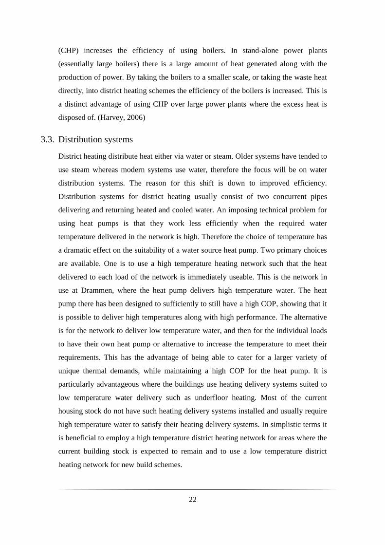
Värtan Ropsten, Stockholm
Largest water source heat pump in the world with a capacity of 180 MW, this is a
seawater heat pump which was completed in 1988. It uses 8 separate heat pump units
which each use the refrigerant R134a haloalkane. This refrigerant is very harmful to
the environment, being hazardous and having a global warming impact 1,410 times
larger than CO2. The system is highly capable of providing a variable output. Each
unit has a 30MW capacity and an ability to downgrade output to 10% of capacity. The
Figure 15: Kingston Heights heat pump system (Smith, 2014)
Page 44
35
heat is fed into the Stockholm district heating scheme with water return and supply
temperatures being around 57°C and 80°C. (Nowacki, 2014)
Figure 16: Largest water heat pump in the world, Värtan Ropsten (Nowacki, 2014)
Page 45
36
COP seasonal variation model 4.2.3.
The seasonal variation in river temperature causes changes in the COP of the
heat pump. A simple model in Excel was created to simulate this variation. It was
assumed that the heat pump is designed to provide the mean COP at the mean river
temperature, and then the COP varies linearly with respect to the variations in
temperature. The variation is taken to be 5% of designed COP per degree variation.
This means that an increase in water temperature by one degree results in a 5%
increase in COP and similarly a one degree decrease results in a 5% decrease in COP.
Figure 17 displays the variation of the COP against the difference between the water
temperature and the annual mean water temperature. Taking the average of this
seasonally varying COP over the entire year gives the SPF. The heat pump design
ultimately dictates the COP variation and instead of modelling this tests could be
performed by the manufacturer to determine sensitivity.
2.5
2.6
2.7
2.8
2.9
3
3.1
3.2
3.3
3.4
3.5
6 5 4 3 2 1 0
CO
P
Δ Mean Temperature
COP vs. Δ Mean Temperature
Figure 17: Seasonal variation of COP, River Clyde
Page 46
37
Figure 18: River source heat pump flow diagram
Page 47
38
4.3. District heating
In the previous sections some technical aspects of a WSHP have been detailed as well
as a look at a few case studies which detail some characteristics of water source heat
pumps in various parts of the world. The design process also depends on the demand
profile the heat pump is accommodating for. Heat pumps can be used to heat an
assortment of needs: individual homes, large tenement blocks, distilleries,
government/council buildings, universities, etc. District heating can be used to
provide a method of connecting the thermal requirements of all of these. This results
in a collective demand profile which needs to be met. As has been discussed, the best
heating system for district heating is likely to be a hybrid system, consisting of
different heating devices. This means that along with the river source heat pump there
will be additional devices covering variability in the load and to provide back up.
Modelling is required to investigate the best fit for a variety of heating configurations
and will be performed by developing an Excel spreadsheet. This will primarily be
used as an exercise in demand/supply matching to examine the various benefits of
different heating supply options.
Determining the demand profile for a district heating scheme can be complicated and
in the following sections a methodology for identifying a potential area suitable for
district heating and producing a basic demand profile for that area will be outlined.
The methodology presented here is not for an accurate prediction of the actual future,
past or present demand profile, but for providing a demand profile realistic enough to
provide useful insight. This section concludes with the relevant flow diagram.
Heat map site identification 4.3.1.
In an effort to promote the implementation of low-carbon heating solutions the
Scottish Government developed an interactive heat map “to visualise and assess who
needs heat, where sources of heat might come from and how these can be connected
in an efficient way to reduce the cost of heat supply and the carbon intensity of heat
generation.” (HeatMap, 2015) It is a Geographical Information Systems (GIS) tool,
containing large datasets capable of providing greater understanding of the potential
for alternative heating. It is a map of Scotland with tools for overlaying information
Page 48
39
regarding heat demand, current heat supplies, geothermal opportunities, social
property ownership percentage and current district heating schemes. The underlying
motivation is to provide a tool capable of highlighting the socio-economic benefits,
which are widely available, of transforming away from traditional methods of heating
to modern, low-carbon ways of heating.
It is most useful for identifying where concentrated areas of heat demand exist. These
are areas which have the greatest potential for installation of district heating. In the
context of river source heat pumps it should be used for identifying the areas along
rivers which suit the capabilities of a heat pump driven district heating scheme.
Figure 19: Heat Map Scotland: Overview of Scotland
Page 49
40
Figure 19 is a snapshot from the heat map providing an overview of the heating
demands spread across the entire country. The scale runs from grey to blue to red,
with red and grey corresponding to a large heating requirement and virtually non-
existent heating demand respectively. It is immediately obvious that the central belt
and east coast regions of Scotland, where most of the population resides, have the
highest density of heating demand.
Figure 20 zooms up on central Glasgow showing the heating demand at the lowest
possible scale of 50 m2. This conveys then resolution power of the heat map. It is
possible to, with a reasonable degree of accuracy, map out areas near to the River
Clyde which are most suitable for district heating. There is a zone selection function
which calculates the total annual heating demand in a user defined area. This allows
selection of a suitable area with a heating demand which a river source heat pump can
drive a district heating scheme for.
Figure 20: Glasgow heating demand map
Page 50
41
The map also contains other valuable tools. It can show where there are installed low-
carbon energy supplies, as shown in figure 21. Another tool displays the operational
(pink) and in development (green) district heating schemes, with the size of the icon
denoting the relative size of the scheme. The percentage of social housing in an area is
shown in the same figure, 22, and is useful because generally district heating is easier
to be agreed upon in these areas.
Figure 21: Heat map, low-carbon technologies, yellow: ASHP, green: Biomass
Figure 22: Heat map, social housing and district heating icons
Page 51
42
Demand profile 4.3.2.
Once an area has been selected from the heat map the next step is to produce a
demand profile over a year. The heat map only provides an annual heating
requirement, which is useful to give a very basic notion of the size of heat pump
which is required. However, it is necessary to consider the seasonal, daily and hourly
fluctuations which will characterise the heating demand profile. This is done by
attempting to distinguish different classes of heating demands in the selected zone.
The chosen classes were domestic dwelling, offices, and retail. Some buildings are
unique so should be treated as an individual class. For a real feasibility study it would
be necessary to attempt to contact the relevant authorities and businesses to obtain a
more accurate heating profile. The heating demand is usually separated between hot
water and space heating. This analysis aims to provide an overview of total heating
requirements, so shall combine the two indiscriminately. Table 2 outlines the various
characteristics of the classes of building.
Table 2: Thermal demand characteristics of building class
Residential Commercial Office
Heating demand zero
during night: 00:00 →
06:00
Heating demand zero
during evening and night:
19:00 → 08:00
Heating demand zero
during evening, afternoon
and night: 12:00 → 07:30
Fairly constant demand:
06:00 → 00:00
Reducing demand from:
08:00 → 19:00
Sharp rise and fall to peak
at 09:30 from 07:30 →
12:00
Gradual seasonal variation Gradual seasonal variation Distinct seasonal variation
Page 52
43
The following graphs show a typical day demand for each of the building classes,
illustrating further the characteristics outlined in Table 2. Note that the residential
profile is based on a three bedroom house. The demands were obtained from the Merit
demand/matching software with half hourly time-steps over a whole year.
0
0.5
1
1.5
2
2.5
3
3.5
4
4.5
0.5 4.5 8.5 12.5 16.5 20.5
Th
erm
al
Dem
an
d (
kW
h)
Half-hour
Day Residential 3 Bedroom Thermal Demand Profile
Figure 23: Residential thermal demand profile
0
0.1
0.2
0.3
0.4
0.5
0.6
0.5 4.5 8.5 12.5 16.5 20.5
Th
erm
al
Dem
an
d (
kW
h)
Half-hour
Day Commercial Thermal Demand Profile
Figure 24: Commercial thermal demand profile
Page 53
44
These demand profiles then need to be accumulated to provide a representation of the
district heating network. The first step is to find the total annual demand of the
proposed area. The heating demands should then be normalised to each other based on
their individual total annual demand. This is because in their original format they all
have different individual total annual demands. The relative ratios of the building
classes should then be estimated based on any information regarding the proposed
area that can be obtained. For example if it is estimated that there is equal proportion
of the three classes then there is a 33.33 : 33.33 : 33.33 relative ratio. The normalised
building classes can then be scaled up such that they account for the total annual
demand of the proposed district scheme. The problem here is that it assumes that each
house will use heat at the exact same time and they will all use a peak heat load at the
same time. In reality the accumulation of thermal demands causes a smoothing of the
demand profile. This is because individual buildings will have slightly different
demand profiles and the differences combine to result in a smoothing effect. To
simulate this, a moving average over 36 half-hour data points is taken. This provides a
demand profile which maintains the characteristics of the individual profiles, while
accounting for the inherent reduced variability of scaling the demand up to the district
scheme level.
0
100
200
300
400
500
600
700
800
0.5 4.5 8.5 12.5 16.5 20.5
Th
erm
al
Dem
an
d (
kW
h)
Half-hour
Day Office Thermal Demand Profile
Figure 25: Office thermal demand profile
Page 54
45
Figure 26: District heating flow diagram
Page 55
46
4.4. Demand/Supply matching
In order to suitably combine the heat pump and the district heating demand it is
necessary to perform demand/supply matching. This was done through the
development of an Excel spreadsheet which essentially compares the supply, the
heating system, and the demand, the district heating. The methodologies for
developing profiles for the district heating demand and the supply profile of the heat
pump have been described earlier. The purpose of the Excel is to bring these two
profiles together. The heating system configuration will be set up in the spreadsheet
and are defined in the following section. A number of technical outcomes are used to
help with sizing a demand to fit the heat pump.
Heating system configuration 4.4.1.
Four heating system configurations were used in the analysis to provide comparisons.
The first two cases do not employ a district heating scheme, individual buildings
provide their own heating through individual heating systems. The other two cases do
have district heating. These incur 2.5% losses due to the piping systems involved.
The base case uses gas boilers to provide all the heating needs. This is taken as the
base case because it is the most common heating setup in the UK. It is easy to set up
as it is presumed that all of the heating needs are met by the individual boilers. They
are high efficiency boilers with η = 80%. (Sun, Wang, & Sun, 2004)
The second base case is a 50:50 mix of individual boilers and electrical heating.
Electrical heating is still prevalent in many outdated homes and therefore needs to be
considered. It is taken that electrical heaters are 100% efficient. This neglects the
inefficient methods by which electrical heaters are employed in homes.
The third case employs solely gas-powered CHP devices. It is assumed that they have
sufficient output variability to meet any change in demand. The heat leads the power
meaning that the power produced by the plants is the by-product and does not try and
match actual electrical demands. It is assumed that all the power produced by the
CHP can be used. The ratio of heat to power was 2:1. This means that for every 2 kWh
Page 56
47
of heat produced, 1 kWh of power is also produced. The efficiency of the CHP is
taken to be 75%. (CarbonTrust, 2010)
The fourth case is made up of a river source heat pump and CHP. The CHP has the
same characteristics as the third case. The technical parameters of the WSHP is
determined by following the methodology given in section ‘4.2 River source heat
pumps’, and is dictated by the specifics of the river, technical limitations, and the
district heating scheme demand needs. Table 3 outlines the technical characteristics of
all four configurations.
Table 3: Heating system configurations of the four cases
Base Case 1 Base Case 2 Case 1 Case 2
Configuration Indiv. Gas
Boilers
Indiv. Gas
Boilers +
Elect. Heating
CHP Only WSHP + CHP
Efficiency 80% 80% + 100% 75% N/A% + 75%
Piping Losses 0% 0% 2.5% 2.5%
To model the effect of choosing between high or low temperature distribution
systems, two different COPs were used in the following demand/supply matching
analysis. For a high temperature distribution system a COP of 3.0 was used and for
the low temperature one a COP of 3.5 was used. These are based on comparative
COPs from case studies and the requirement to qualify for the Renewable Heat
Incentive (RHI) which requires a COP of at least 2.9.
Technical outcomes 4.4.2.
A number of technical outcomes are produced from the Excel spreadsheet to aid the
sizing of the demand to fit the heating system configuration. A simple technical
outcome will be the net electricity consumed by the heating configuration including
the heat pump.
Page 57
48
The average percentage of the capacity of the heat pump utilised (A.C.F.) provides an
insight into whether the heat pump is the correct size to fit various demands. This is
calculated using the following equation.
𝐴. 𝐶. 𝐹. (%) = (𝐻𝑒𝑎𝑡 𝑝𝑢𝑚𝑝 𝑝𝑟𝑜𝑣𝑖𝑠𝑖𝑜𝑛 𝐻𝑒𝑎𝑡 𝑝𝑢𝑚𝑝 𝑐𝑎𝑝𝑎𝑐𝑖𝑡𝑦 𝑜𝑢𝑡𝑝𝑢𝑡) × 100⁄
17520 (= 𝑛𝑢𝑚𝑏𝑒𝑟 𝑜𝑓 ℎ𝑎𝑙𝑓 − ℎ𝑜𝑢𝑟𝑠 𝑖𝑛 𝑎 𝑦𝑒𝑎𝑟)
The percentage of the annual demand provided by the heat pump (P.H.P) gives
another insight into the utilisation of the heat pump device itself. It is calculated using
this equation.
𝑃. 𝐻. 𝑃. (%) = (𝐻𝑒𝑎𝑡 𝑝𝑢𝑚𝑝 𝑝𝑟𝑜𝑣𝑖𝑠𝑖𝑜𝑛 𝐷𝑒𝑚𝑎𝑛𝑑)⁄ × 100
17520 (= 𝑛𝑢𝑚𝑏𝑒𝑟 𝑜𝑓 ℎ𝑎𝑙𝑓 − ℎ𝑜𝑢𝑟𝑠 𝑖𝑛 𝑎 𝑦𝑒𝑎𝑟)
The heating system configuration with the heat pump also includes CHP. It is
important to keep track of what size of CHP is required to compliment the heat pump.
This is done by evaluating the size of CHP unit required by examining the peak load
over the year and including a safety 10% to ensure that the heating demand in an
atypical year can still be met. It is calculated using the equation below.
𝑆𝑖𝑧𝑒 𝐶𝐻𝑃 (𝑀𝑊) = 1.1 × 2 × 𝑀𝑎𝑥 𝐶𝐻𝑃 𝑜𝑣𝑒𝑟 𝑒𝑣𝑒𝑟𝑦 ℎ𝑎𝑙𝑓 − ℎ𝑜𝑢𝑟 𝑜𝑓 𝑡ℎ𝑒 𝑦𝑒𝑎𝑟
1000
Note that in this equation the need for the factor of 2 is to account for the fact that the
timescale is in half-hours.
Page 58
49
4.5. Environmental
One of the main motivations for considering heat pumps is that they are perceived to
be more environmentally friendly than other forms of heating. This section will set
out a methodology for determining the various environmental impacts associated with
heat pumps and district heating networks. It will discuss the legislation and
organisations which must be consulted with regard to the use of water by the heat
pump. The impacts surrounding the construction of the district heating network will
be detailed with a view to formulating a method for mitigating and eliminating such
impacts. Then the issue of air quality and emissions will be addressed and the
procedure for quantifying these will be developed. Addressing the core environmental
principles allow for the formulation of the environmental methodology capable of
further investigating the viability of a district heating network driven by a river source
heat pump.
SEPA regulations 4.5.1.
The principle government body in charge of regulating, improving and protecting
environmental issues in Scotland is the Scottish Environmental Protection Agency
(SEPA) (SEPA, 2015). This means that water issues, and in particular those
pertaining to water source heat pumps, come under SEPA’s jurisdiction. The Water
Environment (Controlled Activities) (Scotland) Regulations 2011 covers the level of
authorisation required for any projects which involve the use of natural water. These
regulations are also known as CAR. Figure 27 outlines the authorising process which
must be followed.
The important areas from the regulations relevant to water source heat pumps are
required licences and subsistence charges. If the scheme abstracts water in excess of
2,000m3
per day then the project requires a ‘Complex License’. This involves a fee of
£2,934 and an application procedure lasting four months. For the pipework and heat
pump structure an ‘Engineering Licence’ would be required as a separate licence from
the ‘Complex Licence’. The fee for this would be £2,000. Subsistence charges can be
avoided by ensuring that the heat pump returns the water it extracts to the same
Page 59
50
location. This should be incorporated into the design of the heat pump to avoid this
extra fee and to ensure compliance of the project with SEPA.
Figure 27: CAR authorisation process
Page 60
51
Construction 4.5.2.
The construction of both the heat pump and district heating network pose a large a
number of potential environmental issues. The main problem comes from the
expensive and far-spread pipe work which needs to be laid out to both take the heat
from the heat pump to the district heat network and for the district heat network itself.
If the central district heating centre is not located at the heat pump then piping will be
required to connect the two. Mapping (for example Google Maps) can be used to
identify an ideal network path as well as a number of alternatives. An example
network is shown in figure 28. Note that bridges are useful for piping across a river.
Then the paths should be analysed from an environmental perspective considering the
brief checklist provided in table 4. This can be performed on foot and ensuring
photographs are taken to assess any issues.
Figure 28: Glasgow, example annotated piping network
Page 61
52
Table 4: Environmental checklist for piping
Heat pump District heating
Routing should use bridges to cross rivers Possible traffic disruption if follows roads
Historical consultation Historical consultation
Drift deposits Disruption to public
Solid deposits Distance from centre
Existing ground conditions Land use
A full environmental impact assessment would be required to determine the full
significance of the various potential impacts. This brief method provides a simple
method for determining the obvious impacts at an early feasibility stage.
Emissions and air quality 4.5.3.
The CO2 equivalent savings are calculated by comparing the CO2 equivalent
emissions of both the energy used by a heat pump and CHP system and that of the
solely CHP system to the base case of individual gas boilers. The first system will use
more electricity than gas, with the heat pumps COP determining CO2 equivalent
savings. The CHP only system will provide CO2 equivalent savings through the
additional production of electricity. The base case will be used to determine the
savings. The following equation defines how CO2 equivalent savings, in kg/yr, are
calculated.
𝐶𝑂2 𝑆𝑎𝑣𝑖𝑛𝑔𝑠 =(𝐸𝐵𝑎𝑠𝑒) × (𝛼𝑔𝑎𝑠)
𝜂𝑏𝑜𝑖𝑙𝑒𝑟− 𝐸𝑚.𝑒𝑚𝑏.− (𝐸𝐶𝑎𝑠𝑒) × (𝛼𝑔𝑎𝑠) − (𝐸𝑔𝑟𝑖𝑑) × (𝛽𝑔𝑟𝑖𝑑)
Where 𝐸𝐵𝑎𝑠𝑒 is the thermal energy produced by the gas used by the base case, in
kWh/yr, 𝛼𝑔𝑎𝑠 is the mass of carbon dioxide equivalent emitted per kWh for natural
gas, in kg, 𝜂𝑏𝑜𝑖𝑙𝑒𝑟 is the efficiency of the individual gas boilers, 𝐸𝑚.𝑒𝑚𝑏. is the
embodied emissions of the chosen case, in kWh, 𝐸𝐶𝑎𝑠𝑒 is the thermal energy of gas
consumed in the chosen case, in kWh/y, 𝐸𝑔𝑟𝑖𝑑 is the net electricity imported to the grid
Page 62
53
(accounting for exports), in kWh, and 𝛽𝑔𝑟𝑖𝑑 is the mass of carbon dioxide equivalent
emitted per kWh for electricity.
The embodied emissions accounts for the carbon dioxide equivalent emissions
associated with the construction and materials involved with the cases. This can prove
particularly difficult as it requires the energy used to build materials for devices and
even then the materials used for a device are not easily obtained. Construction carbon
dioxide equivalent emissions are also difficult to obtain as construction time can vary
even for the same project and there is rarely any monitoring of emissions on-site.
These figures should be obtained where possible.
The CO2 equivalent emissions factors, 𝛼𝑔𝑎𝑠 and 𝛽𝑔𝑟𝑖𝑑, can be obtained from the
Department of Environment, Food & Rural Affairs (DEFRA) who provide a large
variety of emission factors for greenhouse gas reporting (DEFRA, 2015). These are
the figures from the 2015 update. These figures are provided so that companies can
calculate and report their own emissions.
Table 5: CO2 equivalent emission factors for gas
It is important to note that these figures represent the carbon dioxide equivalent factor.
This is the combination of all the emissions which contribute to global warming and
equating them to CO2. According the Kyoto Protocol there are 7 contributory
greenhouse gases: carbon dioxide (CO2), methane (CH4), nitrous oxide (N2O),
hydrofluorocarbons (HFCs), perfluorocarbons (PFCs), sulphur hexafluoride (SF6),
and nitrogen trifluoride (NF3). Each of these has an equivalence factor to CO2 which
is treated as the base measurement for global warming impact.
The UK currently has targets to decarbonise the grid; they are committed to a
greenhouse gas emission reduction of 45% by 2020 and 80% by 2050 (NationalGrid,
2015). This needs to be included in the analysis of carbon savings. It will be presumed
𝜶𝒈𝒂𝒔 𝜷𝒈𝒓𝒊𝒅
0.18445 kg/kWh 0.46219 kg/kWh
Page 63
54
that there will be a linear 12% reduction in the CO2 equivalent emission factor
annually. This means that by 2021 there will 47% reduction in the factor from 2015.
This assumption, perhaps optimistically, expects that governmental targets will be met
in the projected timeframe.
The carbon dioxide equivalent factor does include the effect of a number of global
warming impact greenhouse gases. It is also useful to consider the possible reduction
of emissions which effect air quality. For this section it will be assumed that the
electricity consumption has no effect on air quality, as often the producers of the
electricity are situated away from major cities. Nitrogen oxides and carbon monoxide
are the two emission products which are useful as measures of air quality. Table 6
provides the emission factors for NOX and CO from gas combustion.
Table 6: NOX and SOX emission factors for gas (USEPA, 1995)
NOX CO
0.000062 kg/kWh 0.000142 kg/kWh
Page 64
55
Figure 29: Environmental flow chart
Page 65
56
4.6. Economic
The viability of any project ultimately is decided based on the economics of the
project. Many sustainable projects only go ahead because of expected returns due to
prospects such as incentives or reduced energy cost. Often projects will still go ahead
if there is a large reduction in emissions or environmental impact as this can benefit
companies in reaching overarching goals. This section will discuss the methodology
involved with analysing the financial aspect of installing a district heating network
driven by a river source heat pump. It will detail the eligibility and benefits of the
governmental incentive scheme, the Renewable Heat Incentive. There will be
discussion of the considerations involved with capital costs for both the heat pump
and the district heating network, as well as potential savings (or costs) from
considering operational costs. All of these considerations will be brought together to
perform the economic modelling to investigate the financial viability of a project.
Renewable Heat Incentive (RHI) 4.6.1.
One of the reasons that low-carbon heating technologies are becoming a viable option
in the UK was the introduction of the Renewable Heat Incentive (RHI). This is an
incentive which pays based on how much heat is produced. There are currently two
levels of incentive; non-domestic and domestic. OFGEM outlines a few different
general guidelines to decide which scheme your system would be eligible for.
(OFGEM, 2015a) The following list outlines some of the factors involved.
The renewable heating system heats one home which has an Energy
Performance Certificate then it is likely domestic scheme
Renewable heating system for commercial, public or industrial then likely
non-domestic
“… organisations with district heating schemes where one heating system
serves multiple homes.”
Page 66
57
The last bullet point is the most important in the context of the type of district heating
scheme this thesis looks at. Most similar prospective projects should fall under the
non-domestic scheme.
There are further requirements for a water source heat pump project to qualify for the
RHI.
Minimum COP of 2.9
Minimum SPF of 2.5
Reversible heat pumps can only measure the heating, not cooling
Heat pumps to be sized based on design conditions
For multiple heat pumps, the heat drawn from the water must be measured
Electrical consumption of the heat pump must be monitored
Can only extract heat from natural sources such as solar energy stored
naturally (excluding solar collectors), heat from space heating or cooling or
generally any heat from processes other than heat generation
The last bullet point contains a very important distinction which is underlined. It is
specified that the heat which the heat pump draws upon cannot be from a heat
generation source and must come from natural processes. This means that waste heat
from CHP, industrial processes or power plant thermal excesses cannot be used to
form part of the heat from which the heat pump draws. Care therefore must be taken
that any prospective heat pump does not include waste heat from industrial processes.
The COP and SPF of heat pumps could potentially be increased dramatically if this
was allowed due to the increased temperature of the water. It is uncertain if this is to
be reviewed at a later date with increased pressure to utilise wasted thermal heat.
“5.23. If accredited on or after 24 September 2013, heat loss through external heat
distribution piping (e.g. to transport heat between buildings, or between a standalone
boiler and a building) where the piping is not ‘properly insulated’ or where the piping
is more than 10m in length and the average annual heat loss from the piping is
Page 67
58
calculated as being 3% or more of the projected annual heat output of the plant49 50,
is also not seen as serving an eligible use and as such RHI payments cannot be made
in respect of the heat lost.”
This is an important section from the documentation for its implications for the
district heating scheme. It seems that piping losses must be kept below 3% to remain
qualified for the scheme. Therefore the way that the heat is used in the district heating
scheme is also important for eligibility of the RHI scheme.
The non-domestic RHI scheme continues for 20 years of the lifetime of the heat
pump, with payments made on a quarterly basis. There are two tiers of payments that
make up the payments. The first tier applies to the ‘initial heat’ which is the amount
of heat generated by the heat pump if it was running at capacity for 15% of the year.
Any heat generated on top of this comes under the second tier of payment. Table 7
provides the tariffs that apply for systems with an accreditation on or after the 1st of
July, 2015.
Table 7: RHI Tariffs for WSHP
Capital and operational costs 4.6.2.
One of the most important distinctions to make with regard to the economics of
district heating is between retrofit and new build. New build refers to the situation
where a new housing scheme or district of buildings is being planned and there are
plans to install a district heating scheme. In this case the buildings can be built with
designs which take into consideration of the fact the heating delivery systems are
optimised to suit district heating. Piping can be laid in carefully planned layouts. This
is taken further by the use of a heat pump to drive the heating network. This takes the
argument back to the choice between low and high temperature networks. It is easier
RHI Tariffs for Water/Ground Source Heat Pumps
Tier 1 Tier 2
8.84 p/kWh 2.64 p/kWh
Page 68
59
to construct buildings with heating delivery systems which suit low temperature
district heating networks. This can help reduce the costs associated with the project.
For retrofit it is more expensive to install the heating delivery systems suited to low
temperature heating networks. This means the financial analysis required for such
systems generally should be specific to the existing buildings, as these buildings could
have widely ranging costs for retrofit heating systems. It is easier to consider the
economics of high temperature heating networks for these buildings. This is because
no adjustments are needed for the heating delivery systems.
The costs involved with the cases to be examined broadly fit into three categories:
capital, operational and incentives. A list of the capital costs associated with the heat
pump and the district heating network are given in tables 8 and 9, and operational
costs in tables 10 and 11. They are accompanied by methods for approximating the
cost. Incentives are made up solely by the RHI payments described in the appropriate
section.
Table 8: Heat pump: Capital costs
Component Approximate Cost Method
Heat pump Consider size, use case studies for
comparisons
Pumping system Analyse the required pumping depth of
the river, try to minimise
Building centre Local building heat connection
Electrical connections Analyse the electrical consumption
requirement
Landscaping Depends on the piping work required to
move the heat, river crossings need to be
considered
Licences See the section 4.5.1 SEPA regulations
Design Costs for designing the system
Page 69
60
Table 9: District heating network: Capital costs
Component Approximate Cost Method
Energy centre Consider using existing facilities, also
depends on use of CHP or similar onsite
thermal energy production
Piping connections Needs to be considered building to
building, mapping is required
Local building heat connection Consider demands of building, existing
facilities, and desired heating delivery
system
Table 10: Heat pump: Operational costs
Component Approximate Cost Method
Electrical costs Demand/supply matching allows for
analysis of electrical consumption
Technical maintenance Costs with faults and upgrades, take as
low percentage of capital cost
Cleaning maintenance (filtration system) Depends on sophistication of filtration
system, subject to future change in river
conditions
Trained operators Existing skills may not exist, training
costs may be required
Table 11 District heating network: Operational costs
Component Approximate Cost Method
Trained Operators Existing skills may not exist, training
costs may be required
Technical maintenance Costs with faults and upgrades, take as
low percentage of capital cost
Page 70
61
The methodology proposed regarding the capital and operational costs is useful where
data is available. These would be taken from contact with manufacturers to obtain
specific costs for each of the sections. This proved difficult to achieve in this project.
Particularly difficult to find was operational costs. These have been assumed to be the
same as if using gas boilers because it is assumed that they are a relatively low cost.
As an alternative to the methodology the capital costs are estimated based on the
previous case studies discussed. These estimates are given in table 12.
Table 12: Estimations for costs
Heat Pump District Heating CHP
Capital Cost £1.25 million/MW £2.5million £800 k/MW
Financial model 4.6.3.
The Excel spreadsheet used to perform the technical and environmental components
was also used to develop a financial model. Each of the heating system configurations
were examined from an economical perspective. A result obtained from the technical
analysis is the total electricity and gas consumption. These were then multiplied by
the cost per kWh of each of the respective energy sources. The addition of these two
provides the annual energy cost. This process is applied to each case to obtain the
energy cost of each per annum. Table 13 gives the electricity and gas prices used.
Table 13: Gas and electricity prices
Gas Price, pence per kWh Electricity Price, pence per kWh
0.034 0.1
For the case of the CHP and WSHP the RHI payment can be subtracted from the
costs. This was calculated using the two tier system outlined in the section 4.6.1
Renewable Heat Incentive (RHI). The logic used to calculate the RHI payment is
given below.
Page 71
62
𝐼𝐹 (𝐻𝑒𝑎𝑡 𝑓𝑟𝑜𝑚 ℎ𝑒𝑎𝑡 𝑝𝑢𝑚𝑝 𝑎𝑛𝑛𝑢𝑎𝑙)
≥ (15% 𝑜𝑓 ℎ𝑒𝑎𝑡 𝑐𝑎𝑝𝑎𝑐𝑖𝑡𝑦 𝑤𝑜𝑟𝑘𝑖𝑛𝑔 𝑎𝑙𝑙 𝑦𝑒𝑎𝑟)
𝑇𝐻𝐸𝑁 (𝑇𝑖𝑒𝑟 1 𝑝𝑟𝑖𝑐𝑒) × (15% 𝑜𝑓 ℎ𝑒𝑎𝑡 𝑐𝑎𝑝𝑎𝑐𝑖𝑡𝑦 𝑤𝑜𝑟𝑘𝑖𝑛𝑔 𝑎𝑙𝑙 𝑦𝑒𝑎𝑟)
𝐼𝐹𝑁𝑂𝑇 𝑇𝐻𝐸𝑁 (ℎ𝑒𝑎𝑡 𝑓𝑟𝑜𝑚 ℎ𝑒𝑎𝑡 𝑝𝑢𝑚𝑝 𝑎𝑛𝑛𝑢𝑎𝑙) × (𝑇𝑖𝑒𝑟 1 𝑝𝑟𝑖𝑐𝑒)
+
𝐼𝐹 (ℎ𝑒𝑎𝑡 𝑓𝑟𝑜𝑚 ℎ𝑒𝑎𝑡 𝑝𝑢𝑚𝑝 𝑎𝑛𝑛𝑢𝑎𝑙)
≤ (15% 𝑜𝑓 ℎ𝑒𝑎𝑡 𝑐𝑎𝑝𝑎𝑐𝑖𝑡𝑦 𝑤𝑜𝑟𝑘𝑖𝑛𝑔 𝑎𝑙𝑙 𝑦𝑒𝑎𝑟)
𝑇𝐻𝐸𝑁 𝑧𝑒𝑟𝑜
𝐼𝐹𝑁𝑂𝑇 𝑇𝐻𝐸𝑁 ((ℎ𝑒𝑎𝑡 𝑓𝑟𝑜𝑚 ℎ𝑒𝑎𝑡 𝑝𝑢𝑚𝑝 𝑎𝑛𝑛𝑢𝑎𝑙)
− (15% 𝑜𝑓 ℎ𝑒𝑎𝑡 𝑐𝑎𝑝𝑎𝑐𝑖𝑡𝑦 𝑤𝑜𝑟𝑘𝑖𝑛𝑔 𝑎𝑙𝑙 𝑦𝑒𝑎𝑟)) × (𝑇𝑖𝑒𝑟 2 𝑝𝑟𝑖𝑐𝑒)
A relative saving was found by comparing the costs to the two base cases for the CHP
only and CHP + WSHP cases. These savings were then used in a discounted cash
flow (DCF) model(Olsson & Levin, 2015). This model is uses the concept of time
value of money to provide a more realistic view of the savings possible by
implementing a project. Future expected savings are discounted to account for the
perspective that future cash flows are worth less than cash flows closer to the present.
The following equation calculates the discounted present value (DPV), the discounted
future cash flow.
𝐷𝑃𝑉 = 𝐹𝑉
(1 + 𝑟)𝑡
Where FV is the expected cash flow value in a future block of time, r is the discount
rate, and t is the years in the future that the cash flow is expected to occur. This
formula was used for each year and then each case was summed to calculate the DPV
for a certain number of years. Generally the lifetime of a WSHP is expected to be at
least 20 years, so this is the number used in the financial model. A discount factor of
4% was used. Comparing the DPV over the whole 20 years to the capital cost for each
of the cases means that a payback period can be calculated. Payback periods are an
essential part of the feasibility of any project so that investors can know when to
expect their investments to being to bring cash flows.
Page 72
63
Each of the cases was compared using the above financial model. This methodology,
in conjunction with the technical methodology, allows for a variety of different
possible heating configurations to be compared. Importantly it allows for the
inspection of the feasibility of a river source heat pump from a financial perspective.
Page 73
64
Figure 30: Economic flow chart
Page 74
65
5. Results & Analysis
The developed methodology will now be applied to an area of Glasgow using the
River Clyde as the source of heat for the heat pump. The focus is on the core areas of
technical, environmental and economic. The suitability of the River Clyde will be
assessed and the size of heat pump which could be used will be calculated. The
Scotland Heat Map will be used to identify an area of Glasgow potentially suited for a
large district heating scheme, with emphasis on exploring which size of demand fits
well with the proposed heat pump. The modelling focusses on demand/supply
matching for various heating system configurations and proposed sizes of district
heating demand. An assessment of the environmental impacts and economic
comparisons will help determine the various pros and cons of the different heating
system configurations, particularly the WSHP and CHP hybrid system.
5.1. River Clyde suitability
A large dataset obtained from SEPA from 01/10/1963 to 30/09/2014 from the Clyde
at Daldowie station was used to produce the flow rate exceedance curve. This is
shown in graph 31. The percentage of time, over the dataset period, a large range of
flow rates are exceeded is plotted against the flow rate to be exceeded. It was decided
that a flow rate of 8 m3/s was the highest suitable flow rate that could be used for the
heat pump. This is because the curve begins to dip below 99% beyond this point and
since the heat pump needs to provide heat for most of the year in a climate such as
Scotland’s, anything below 99% would have a dramatic effect on the ability of the
heat pump to deliver. Since it is unfeasible to take all of the 8 m3/s flow and also that
there is little guidance from SEPA on abstraction allowances, it was assumed that for
the River Clyde the maximum extraction would be 10%. This means that the heat
pump can utilise a flow rate of 0.8 m3/s.
It should be noted that the Clyde at Daldowie station is not located in the centre of
Glasgow. It is closer to the outskirts of the city. Therefore there is a risk that the flow
exceedance curve is unreliable. It has been assumed that the topology of the river is
relatively unchanging through the city, meaning that the flow rate is also reasonably
constant and so the data from Daldowie can be representative of the data in the centre.
Page 75
66
As suggested earlier, it is important to take independent measurements at the
proposed site to achieve the highest accuracy.
The River Clyde is a large, fast flowing river, and thus the high level of flow rate
found for 99% of the time makes it particularly useful for a river source heat pump.
Its location running through the heart of Glasgow provides ample opportunity for the
use of a district heating scheme.
It is more difficult to obtain useful data concerning the river temperature. SEPA does
take water temperature measurements at some of their river stations, but this data was
not available for the River Clyde. Instead the Clyde Sea temperatures were obtained
to provide an insight into what the temperatures can be found on the River Clyde.
Graph 32 displays the monthly average temperatures found in the Clyde Sea. The red
line and the blue line denote the temperatures found at the surface layer (0-10m) and
the bottom layer (40m-seabed). Given the uncertainty of assuming correlation
between the Clyde Sea temperature and that of the River Clyde the lower temperature
bottom layer data was used. With these temperatures, the River Clyde appears highly
0
10
20
30
40
50
60
70
80
90
100
1 5 9
13
17
21
25
29
33
37
41
45
49
53
57
61
65
69
73
77
81
85
89
93
97
101
105
109
113
Per
cen
tag
e o
f ti
me
the
flo
w r
ate
is
exce
eded
Flow rate (m3/s)
Percentage of time over the dates 01/10/1963 to 30/09/2014 the
flow rate (m3/s) is exceeded
99% of the time, 8 m3 /s flow rate
Figure 31: Flow exceedance curve for the River Clyde
Page 76
67
promising as a source for the heat pump. Since temperatures do not dip below 6°C, a
ΔT of 4°C would be possible. Given the uncertainty of the data being used, a more
conservative ΔT of 2°C was assumed possible. This is in line with WSHPs currently
in use.
5.2. Heat pump size
The following equation can be used to calculate the heat which can be drawn from the
river and used by the heat pump.
𝑄𝑖𝑛 = 𝑚 ̇ 𝜌 𝐶𝑝 ∆𝑇
From the previous results regarding the River Clyde the flow rate is 0.8 m3/s and the
ΔT is 2°C. The density of water is 1000 kg/m3 and the specific heat capacity is 4200
J/ kg °C (M. J. Moran, Shapiro, Boettner, & Bailey, 2010).
𝑄𝑖𝑛 = 0.8 × 1000 × 4200 × 2 = 6720000 𝑊
Accounting for the 99% availability of the 8 m3/s flow rate introduced a factor of
0.99.
= 6720000 × 0.99 = 6.65 𝑀𝑊
Therefore the proposed heat pump size is 6.65 MW. This is realistic when compared
to the case studies of functioning heat pumps. The heat pump system in the town of
Drammen delivers 15 MW of heat, and that consists of three components. A 6.65 MW
size is comparable to the 5 MW individual system currently operating at Drammen,
suggesting that this is a feasible size. A heat pump delivering 6.65 MW of thermal
power over a year could provide 58.3 GWh. In combination with another heating
Figure 32: Monthly temperature data, Clyde Sea (ScottishGovernment, 2012)
Page 77
68
device, a hybrid system could provide even more heat than this. The chosen heat
pump would use an open-loop design because of the size of the River Clyde.
5.3. District heating site
The Scotland heat map was used to identify a possible area of central Glasgow near
the River Clyde which could benefit from district heating. Figure 33 is a screenshot of
the centre of Glasgow with the heating demands overlaid. There are a number of areas
with a large proportion of red squares, which signify a large heating demand.
A number of different areas could be suited for district heating. These are close to the
river meaning that potential losses from piping are minimised. Figure 34 shows the
site which was chosen as a potential location for the district heating scheme. It covers
a large part of the Merchant City area of Glasgow, including a shopping centre, St
Enoch’s, a subway station, the courts, and City Halls. This area also has an abundance
of streets connecting in an organised, grid fashion. This would be useful for planning
the layout of the piping networks. There is also often ongoing construction, with old
buildings being replaced by modern ones. This means that the impact of additional
disruption from the construction of the scheme would be lessened. The number of
buildings which will not be replaced outweighs the number that will. In terms of the
Figure 33: Central Glasgow heating demands
Page 78
69
distribution system of the network, it would be sensible to employ a high temperature
system capable of satisfying the needs of the heating delivery systems of older
buildings. The proposed area also contains a large stretch of the River Clyde. This is
useful for broadening the potential locations for the heat pump, increasing the
likelihood of finding a suitable site.
The heat map provides the annual demand of a selected area. The proposed area has
an annual demand of 104 GWh. This is just under twice the heat pump’s maximum
output of 58.3 GWh in a year. It is unrealistic to assume that the entire heating
demand will be connected to the district heating scheme. Graph 35 shows the overlay
of the social housing percentage of the proposed area. Areas of darker blue have a
higher percentage of social housing. Compared to other areas of Glasgow this is
relatively low. This is a weakness of choosing this area for district heating as with
social housing it is easier to find an agreement to connect to the network. This means
that the real heating demand of the district heating network will be significantly less
than the total of the area. In the technical, environmental and economic analysis a
range from 25 to 100 GWh annual demands was compared. This gave an indication of
what annual demand will suit the proposed heat pump.
Figure 34: Proposed area for district heating
Page 79
70
The ratio of building classes is required to develop the thermal demand profile for the
proposed area. This was done by inspection both through maps and through
familiarity of the area. It was estimated that the ratio of residential : commercial :
offices is 50 : 20 : 30. This is a rough estimate. A proper, detailed inspection of maps
of the area is required to obtain a more accurate ratio. However, for the purposes of
this investigation, where the demand profile will not be drastically different with a
different choice of ratio, the estimated was deemed sufficiently realistic.
Figure 36 is the resulting demand profile from following the methodology. The blue
line is the un-averaged demand profile and the red line is where a 36 moving average
has been applied. It is apparent that the choice of moving average provides a
smoother, more realistic demand profile. Daily characteristics are evident with half-
hourly variations still visible and the seasonal variation is also apparent as the profile
exhibits the characteristic U-shape over the year. There is a minimum in summer and
a maximum in the winter.
Figure 35: Social housing percentage for proposed area
Page 80
71
These results convey the suitability of the heat map as a tool for identifying potential
areas for district heating. It does not have the data to provide an accurate profile for
the demand, but by giving the annual demand it offers a basis for developing an
adequate demand profile for use in investigating river source heat pumps in district
heating.
0
5000
10000
15000
20000
25000
30000
35000
Ha
lf-h
ou
rly
th
erm
al
ener
gy
dis
tric
t u
se (
kW
h)
Half Hour
Half-hourly thermal energy district use (kWh) vs
Half-hours for one year
Figure 36: Thermal demand profile of proposed site
Page 81
72
5.4. Demand/Supply matching
The developed demand profile was then used in the Excel spreadsheet to perform
demand/supply matching. The different heating system configurations were compared
using the technical outcomes outlined in the methodology, with special importance for
comparing these systems to the river source heat pump and CHP hybrid system.
Emphasis was placed on analysing the performance of the configurations for different
total annual demands.
An important part of the reason for the promotion of using heat pumps is to move
thermal energy production away from reliance on gas and onto electricity. Heat
pumps then have the advantage over conventional electrical heating with COPs in
excess of 100%. Graph 37 shows the net electricity consumption of the gas and
electricity case and the WSHP and CHP case against the total annual demand of the
district heating scheme.
Figure 37: Electricity consumption vs. Annual demand
For the Gas and Electricity case the trend is linear, as total annual demand increases
the annual electricity consumption proportionally increases. A different trend occurs
with the WSHP and CHP case. For total annual demands up to 40 GWh the electicity
-20.00
-10.00
0.00
10.00
20.00
30.00
40.00
50.00
60.00
25 30 35 40 45 50 55 60 65 70 75 80 85 90 95 100
Net
an
nu
al
ele
ctri
city
co
nsu
mp
tio
n (
GW
h)
Total Annual Demand (GWh)
Net Electricity Consumption (GWh) vs. Total Annual
Demand (GWh)
WSHP + CHP
Gas + Elect.Maximal electricity use
Zero consumpion
Page 82
73
consumption increases. Beyond this the trend reverses and it decreases, with an
inverse linear relationship forming for total annual demands larger than 55 GWh.
In the model the heat pump is always the same size but the CHP varies depending on
what demand the heat pump cannot cover. Therefore for low demands the heat pump
is being utilised more and more, until it cannot provide any more of the heat and the
CHP must be increased to compensate. This results in a larger use of CHP, and
consequently a larger production of electricity. At 80 GWh the electricity produced
becomes larger than the electricity consumed by the heat pump. It appears that the
maximal use of electricity over gas is around 40 GWh.
It is difficult to conclude at which annual demand the heat pump’s use is maximised.
One of the technical outcomes, which helps achieve this, was to calculate the average
capacity of the WSHP used over a year. Graph 38 shows this as a percentage against
the total annual demand.
Figure 38: Percentage of capacity of WSHP used vs. Annual demand
The average capacity used increases as the total annual demand increases. This is
logical because there will be more half-hours where the demand is larger when the
0
10
20
30
40
50
60
70
80
90
100
25 30 35 40 45 50 55 60 65 70 75 80 85 90 95 100
Av
era
ge
cap
aci
ty o
f W
SH
P u
sed
ov
er a
yea
r
(%)
Total Annual Demand (GWh)
Average capacity of WSHP used over a year (%) vs.
Total Annual Demand (GWh)
Page 83
74
annual demand is larger. This means the heat pump is required to produce more heat,
despite the concurrent increasing size of the CHP.
It appears ideal to try and optimise the average capacity used, so this would lead to
the conclusion that a higher total annual demand is desrieable. However, the size of
the CHP required increases accordingly with a higher total annual demand. Graph 39
shows the capacity of CHP required against the total annual demand. The linear
relationship has a steep gradient. This means an increase in the total annual demand
has a large effect on the size of the CHP necessary to meet the demand. A 5 GWh
increase in total annual demand results in an increase of 1.5 MW of required CHP
capacity. Installing a CHP unit so large such that it dwarfs the size of the WSHP
defies the reasoning for including the WSHP at all. It is important that the WSHP
provides a large proportion of the annual heat demand.
Figure 39: Capacity of CHP required vs. Annual demand
0
5
10
15
20
25
25 30 35 40 45 50 55 60 65 70 75 80 85 90 95 100
Ca
pa
city
of
CH
P R
equ
ired
(M
W)
Total Annual Demand (GWh)
Capacity of CHP Required (MW) vs. Total Annual
Demand (GWh)
gradient = 1.5 MW/GWh
Page 84
75
Figure 40: Percentage of demand provided by WSHP vs Annual demand
Graph 40 helps by showing the percentage of the annual demand which is met by the
WSHP against the total annual demand. For a low demand of 25 GWh the entire
annual demand can met by the heat pump with this dropping to 65.8% for a demand
of 100 GWh.
In reality the heat pump will only be able to vary its output to a limited degree which
affects the COP of performance. From this point of view it is important to choose an
annual demand such that the heat pump provides a large proportion of the heat, but
not all. Such a system is acting more like a real one would, with the heat pump
providing the base load and the CHP meeting the fluctations.
The low temperature and high temperature distribution systems were also compared
for different total annual demands. Graph 41 shows this comparison with the
electricity consumption of both plotted against the total annual demand. Since the low
temperature system has a higher COP it is logical that it requires smaller electricity
consumption annually. This confirms the logic that low temperature systems perform
better technically.
0
20
40
60
80
100
120
25 30 35 40 45 50 55 60 65 70 75 80 85 90 95 100
Per
cen
tag
e o
f D
ema
nd
Met
by
WS
HP
(%
)
Total Annual Demand (GWh)
Percentage of Demand Provided by WSHP (%) vs.
Total Annual Demand (GWh)
100%
65.8%
Page 85
76
Figure 41: Distribution systems vs. Annual Demand
-20
-15
-10
-5
0
5
10
15
25 30 35 40 45 50 55 60 65 70 75 80 85 90 95 100
Net
Ele
ctri
city
Co
nsu
mp
tio
n (
GW
h)
Total Annual Demand (GWh)
Comparison of distribution systems: Low temperature
and High temperature
Low Temperature
High Temperature
Page 86
77
5.5. Environmental impact
SEPA regulations state that if the abstraction rate exceeds 2,000 m3 per day a
‘Complex Licence’ is required. Using the 0.8 m3/s flow rate gave a daily flow rate of
68,120 m3/s. This is far in excess of SEPA guidelines, meaning that a ‘Complex
Licence’ is required.
The environmental methodology also sets out a rough environmental impact
assessment process. This was not carried out for this project, but it is possible that this
could be a potential barrier. There were also no embodied emissions calculations
performed for this project. This was due to insufficient data.
Graph 42 displays the CO2 equivalent emissions versus the annual total demand. The
order of the cases in terms of CO2 emissions from lowest to highest is as follows:
CHP only, CHP + WSHP, Gas Boilers and Gas + Electricity. This is because the CHP
generates electricity along with heat, resulting in a reduction in the electricity
imported and hence the net CO2 emissions. All the cases have a simple linear
relationship to the annual demand, with the highest gradients belonging to the highest
emitters.
Figure 42: Comparison of cases: CO2 emissions vs. Annual demand
0
5000
10000
15000
20000
25000
30000
35000
40000
25 30 35 40 45 50 55 60 65 70 75 80 85 90 95 100
CO
2 E
qu
iva
len
t E
mis
sio
ns
(to
nn
es/y
r)
Annual Total Thermal Demand (GWh)
CO2 Equivalent Emissions (tonnes/yr) vs. Annual
Demand (GWh)
Gas Boilers
CHP Only
CHP + WSHP
Gas + Elect.
Page 87
78
The CO2 equivalent emissions were calculated for all of the cases with an annual
demand of 40 GWh. The previous graph used CO2 emission factors from the current
year, 2015. The predicted future trend of decarbonisation of the electricity grid will
have a large impact on the environmental impacts of the various cases. This is shown
in graphs 43 and 44, where the CO2 equivalent emissions vs. year is plotted. The first
uses a decarbonisation factor of 10%, which is line with current UK government
targets. It is in the year 2016, in just over one year, that the CO2 emissions from the
CHP system rise above those of the CHP + WSHP system. This shows that this
system is better as a long-term environmentally friendly heating system. Interestingly,
the CHP system not only exceeds the CHP + WSHP system quickly, after 6 years it is
the highest emitter of CO2. This shows that while CHP is seen to be an
environmentally friendly option in 2015; in the longer term it becomes
environmentally worse than even gas boilers. Graph 44 uses a decarbonisation factor
of 5%. Even with such a pessimistic view of the future decarbonisation of the grid it is
still in less than two years that the CHP + WSHP case has less CO2 emissions than the
CHP only case. In 10 years the cases of CHP only, Gas Boilers and Gas + Electricity
almost converge.
Figure 43: Projected CO2 Emissions: Decarbonisation factor 10%
0
2000
4000
6000
8000
10000
12000
14000
16000
CO
2 E
qu
iva
len
t E
mis
sio
ns
(to
nn
es/y
r)
Year
CO2 Equivalent Emissions (tonnes/yr) vs. Year
Gas Boilers
CHP Only
CHP + WSHP
Gas + Elect.
Decarbonisation
Factor 10%
Page 88
79
With the commitment of the UK government to the decarbonisation of the electrical
grid it appears essential for heating systems to move away from gas and to electrical
based systems, if they wish to reduce CO2 emissions. WSHPs provide the best system
for making the most of the electricity that is used to provide heat.
Figure 44: Projected CO2 Emissions: Decarbonisation factor 5%
The move away from gas to electricity also helps with air quality. Graph 45 and 46
show the NOx and CO emissions of the different cases for annual demands. They both
follow the same trend with the only difference being that there is a higher factor of
CO emissions. CHP is the worst offender in terms of air quality. This is because both
the gas and electricity are being produced in the city. Using more electricity is better
as can be seen with the Gas + Electricity and WSHP + CHP cases being the lowest
offenders for air quality. The WSHP + CHP case has lower emissions than the Gas +
Electricity case up to 70 GWh. This highlights the idea that using CHP causes worse
problems than the other heating devices.
0
2000
4000
6000
8000
10000
12000
14000
16000
CO
2 E
qu
iva
len
t E
mis
sio
ns
(to
nn
es/y
r)
Year
CO2 Equivalent Emissions (tonnes/yr) vs. Year
Gas Boilers
CHP Only
CHP + WSHP
Gas + Elect.
Decarbonisation
Factor 5%
Page 89
80
Figure 45: Air quality, NOx emissions
Figure 46: Air quality, CO emissions
0
2
4
6
8
10
12
14
16
25 30 35 40 45 50 55 60 65 70 75 80 85 90 95 100
NO
x E
qu
iva
len
t E
mis
sio
ns
(to
nn
es/y
r)
Annual Total Thermal Demand (GWh)
NOx Emissions (tonnes/yr) vs. Annual Demand (GWh)
Gas Boilers
CHP Only
CHP + WSHP
Gas + Elect.
0
5
10
15
20
25
30
35
25 30 35 40 45 50 55 60 65 70 75 80 85 90 95 100
CO
Eq
uiv
ale
nt
Em
issi
on
s (t
on
nes
/yr)
Annual Total Thermal Demand (GWh)
CO Emissions (tonnes/yr) vs. Annual Demand (GWh)
Gas Boilers
CHP Only
CHP + WSHP
Gas + Elect.
Page 90
81
The low temperature and high temperature distribution systems were also compared
with respect to their CO2 equivalent emissions, as shown in graph 47. The results
confirm the expectation that low temperature distribution systems will have lower
emissions due to the higher COP.
Figure 47: CO2 emissions: Distribution systems
0
2000
4000
6000
8000
10000
12000
14000
16000
25 30 35 40 45 50 55 60 65 70 75 80 85 90 95 100CO
2 E
qu
iva
len
t E
mis
sio
ns
(to
nn
es/y
r)
Annual Demand (GWh)
CO2 Equivalent Emissions for High Temperature and
Low Temperature Distribution Systems
Low
Temperature
High
Temperature
Page 91
82
5.6. Economic comparisons
The RHI payments have a large impact on the economic viability of the WSHP.
Graph 48 shows the difference in annual cost vs the total annual demand. With the
RHI payments instead of an annual cost there is a payment for annual demands under
60 GWh. To illustrate the difference, for an annual demand of 40 GWh there is an RHI
payment of £1.50 million. The viability of a WSHP is therefore heavily dependent on
this payment. This raises the question of over reliance on this payment. If for some
reason this government subsidy is scrapped or if it is vastly reduced, then the
economics of a WSHP becomes uncertain.
Figure 48: With and without RHI payments comparison
The annual costs of implementing the two cases, CHP + WSHP and CHP only, were
compared to the annual costs of the two base cases, Gas only and Gas + Electricity, to
calculate the relative annual savings. The annual savings relative to the base cases vs.
the total annual demand are shown in graph 49. Greater savings are to be made
upgrading from the Gas + Electricity case than the Gas only case. For higher total
annual demands the savings when upgrading from Gas + Electricity increases at a
-0.50
0.00
0.50
1.00
1.50
2.00
2.50
25 30 35 40 45 50 55 60 65 70 75 80 85 90 95 100
An
nu
al
Co
st (
£m
illi
on
s)
Total Annual Demand (GWh)
With/Without RHI Payments: Annual Cost (£millions)
vs. Total Annual Demand (GWh)
Non-RHI
RHI£1.50 million
Page 92
83
larger rate than the Gas only base case. For both comparisons the CHP + WSHP case
results in larger savings than the CHP only case.
Figure 49: Annual savings of cases vs. Annual demand
The environmental results favoured a move towards electric forms of heating.
Economically it is possible to obtain larger savings by moving away from electrical
heating, but only in the case of conventional electrical heating. It is better to use
WSHPs compared to CHP. This analysis only looks at the savings which can be made
each year, later analysis will include the capital costs to present results which are
better suited to investigating financial availability.
Graph 50 compares the annual costs of the low and high temperature distribution
systems. The low temperature system always has an annual cost lower than that of the
high temperature system. It is interesting how much of a difference there is. The low
temperature system provides payments, as opposed to costs, for annual demands
lower than 90 GWh compared to 55 GWh for the high temperature system. For a 40
GWh annual demand there is a £190,000 saving.
0.00
1.00
2.00
3.00
4.00
5.00
6.00
7.00
8.00
25 30 35 40 45 50 55 60 65 70 75 80 85 90 95 100An
nu
al
Sa
vin
gs
Rel
ati
ve
to B
ase
ca
se
(£m
illi
on
s)
Total Annual Demand (GWh)
Annual Savings Relative to Gas Base Case and
Gas+Elec. Base Case (£millions) vs. Total Annual
Demand (GWh)
CHP Only
CHP + WSHP
CHP Only
CHP + WSHPGas Base
Case
Gas+Elec.
Base Case
Page 93
84
This suggests that the difference paying the extra cost for a low temperature
distribution system could be worthwhile. Due to difficulty in estimating the cost
difference between the systems this analysis was not included, but would be an
interesting avenue for future work. It does show the economic value that district
heating has for new build areas. It makes sense to design homes to suit a distribution
system which also suits district heating, to ensure that this form of heating delivery is
optimised. This is an area worthy of further research.
The discount cash flow model was applied to each of the cases for a total annual
demand of 40 GWh. Graph 51 shows the discounted present savings vs the year for
the two cases CHP only and CHP + WSHP relative to the gas base case. The relative
savings are always larger for the CHP + WSHP system than for the CHP only system.
This model allows for the calculation of the number of payback years. For the CHP
only case there was a payback period of 11.66 years and for the CHP + WSHP there
was a payback period of 9.79 years. This is despite the CHP + WSHP having higher
capital costs. Because of the higher annual savings the payback period is still smaller
than that for CHP only.
-0.5
-0.4
-0.3
-0.2
-0.1
0
0.1
0.2
0.3
0.4
0.5
25 30 35 40 45 50 55 60 65 70 75 80 85 90 95 100
An
nu
al
cost
(£
mil
lio
ns)
Total Annual Demand (GWh)
Low-T and High-T Distribution Systems: Annual cost
(£millions) vs. Total Annual Demand (GWh)
Low-T
High-T
£190,000
Figure 50: Distribution systems: Annual cost vs. Annual demand
Page 94
85
Figure 51: Discounted cash flow, Comparison to Gas
Similar calculations were performed using Gas + Electricity as the base case. The
CHP + WSHP case still offer larger relative annual savings. The difference is that
they are larger, with the payback period for the CHP only case now 5.46 years and for
the CHP + WSHP it is 5.36 years. This emphasises the advantage of installing the
CHP + WSHP case when there is conventional electrical heating. These payback
periods should be considered when compared to the lifetimes of for both systems
around 20 years.
0
0.2
0.4
0.6
0.8
1
1.2
1.4
1.6
1.8
2
201
6
201
7
201
8
201
9
202
0
202
1
202
2
202
3
202
4
202
5
202
6
202
7
202
8
202
9
203
0
203
1
203
2
203
3
203
4
Sa
vin
gs
Rel
ati
ve
(£m
illi
on
s)
Year
Relative to Gas Base Case, Discounted Cash Flow:
Savings Discounted Present Value
CHP Only
CHP + WSHP
Payback:
9.79 Years
Payback:
11.66 Years
Page 95
86
Figure 52: Discounted cash flow, Comparison to Gas + Elec.
0
0.5
1
1.5
2
2.5
3
3.5
201
6
201
7
201
8
201
9
202
0
202
1
202
2
202
3
202
4
202
5
202
6
202
7
202
8
202
9
203
0
203
1
203
2
203
3
203
4
Sa
vin
gs
Rel
ati
ve
(£m
illi
on
s)
Year
Relative to Gas+Elec. Base Case, Discounted Cash
Flow: Savings Discounted Present Value
CHP Only
CHP + WSHP
Payback:
5.36 Years
Payback:
5.46 Years
Page 96
87
6. Conclusions
The main aim of this thesis was to investigate the different aspects concerning large
heat pumps capable of driving a district heating network, and particularly at the case
of implementing one on the River Clyde in Glasgow. The success of the methodology
and the results obtained from it are discussed here. The thesis ends with a section on
suggestions of further work which could be done in this area.
6.1. Methodology
The methodology developed proved to be an apt tool for investigating the case of the
River Clyde, Glasgow. The section concerning the properties of the river provides
useful suggestions for how to best utilise a river as a heat source. The method of
obtaining and analysing the flow rate data is thorough enough to be applied to most
rivers in the UK. The method suggested to obtain the river temperature data is useful
for when this elusive data is unavailable. There could be a more thorough description
of the best practice for performing the required work to obtain the river temperatures.
This applies for the flow rate too.
The heat pump sizing section of the methodology describes a variety of methods for
reducing the size of the heat pump. This section could be developed to include a
model for designing a heat pump, as this is what is required to properly size a heat
pump. This was outside the scope of this project. The following section detailing
more case studies regarding heat pumps is vital without the necessary method of heat
pump design. This is so that realistic estimates of a proposed heat pump can be made.
Ideally, this section would be used to validate the results of a heat pump design
model. For the purposes of this thesis it was sufficient to obtain the relevant technical
characteristics of a heat pump from the case studies. A COP seasonal variation model
was described to account for the seasonal variation in the performance of the heat
pump. It is a simply model, with simplistic assumptions. However, it proved useful as
a means to include this characteristic of heat pump performance, without having the
specifics of the heat pump design. Further work could be performed to more
accurately model this.
Page 97
88
The next section of the methodology described identifying a potential district heating
site and a method of developing an appropriate thermal demand profile. The heat map
proved to be a useful tool for identifying potential areas through high resolution data
on demands and additional tools capable of showing relevant information. Once a site
was selected then the method for generating the demand profile was effective. A
whole thesis could be dedicated to the specifics of generating accurate demand
profiles, but the developed method provided a way of providing a sufficiently realistic
method to be used to test the validity of a WSHP. There could especially be
improvements to the number of building classes included, as it is unrealistic to fit
certain buildings into a choice of only three categories. More data could be included
into the heat map such as seasonal, or even daily, variations of certain areas, or access
to the types of buildings in a certain area. This sub-section ends with the description
of the model used to model the effect of the choice between high and low temperature
distribution system. The reality of this area of district heating is highly complex, and
outside the scope of this project. The model provided a useful method of inspecting
the general difference.
The demand/supply matching required the development of an Excel spreadsheet
model. This model essentially compares the demand of the district heating scheme
and the thermal supply of different heating configurations, four of which were chosen.
The choice of configurations were useful to see how a WSHP could perform in a
hybrid system, as it is unlikely a heat pump would be designed to provide all the
demand. It is also unlikely that the CHP would be used as the only form of top up to
the heat pump. More configurations should be analysed with particular interest in
solar-assisted heat pumps. The model itself would benefit from including a form of
control scheme. This will discussed further in the Further Research section.
The environmental section provided a worthwhile guide for investigating these
concerns. The regulation description is thorough and provides specific details
regarding relevant aspects. The construction section gives a rough environmental
checklist for assessing the environmental impact. For an initial feasibility stage this is
sufficient, but it would be necessary to carry out a much more specific analysis of the
Page 98
89
impacts for a later stage. These specifics are too in-depth for the scope of this thesis.
The carbon emissions and air quality calculations set out provide an effective way of
quantifying these particular environmental aspects. The one area which could be
expanded upon is calculating the embodied emissions associated with construction.
The requirement is for details regarding the components and materials used in
construction of both the heat pump and the district heating.
The economic section begins with a comprehensive description of the RHI regulations
relevant to the project. The capital and operational costs are then discussed, assigning
an approximate cost method to the various components associated with the heat pump
and district heating network. This method is cumbersome, however provides an
effective way of calculating costs in the absence of real data. Even this method
requires a level of data which is difficult to obtain so an alternative is provided using
estimations based on previous case studies. This is adequate for investigating the
economic factors. The financial model uses well sourced electricity and gas prices,
and thorough calculations with the discount cash flow model.
There are limitations to the methodology which this thesis presents. However, they
are often overcome by sensible estimations and alternative, albeit simpler, methods.
The methods proposed are generally applicable to rivers, particularly those in
Scotland. It achieves the objective of developing a generic methodology capable of
investigating the viability of river source heat pumps driving a district heating
network, while addressing technical, environmental and economic aspects.
6.2. Results & Analysis
The River Clyde was found to be a suitable source of heat for a heat pump capable of
driving a district heating network. The analysis of the flow rate showed how the river
is a fast flowing river with more than enough volume to provide for a large-scale heat
pump. The river temperature data used was for the Clyde Sea and therefore very
conservative measures were taken with respect to the viability of this aspect of the
river. Judging by the Clyde Sea temperatures it is possibly feasible for the River
Clyde to provide a higher ΔT than assumed, and therefore a higher heat input. Work
Page 99
90
should be done to take the necessary measurements to confirm this. The proposed heat
pump was sized to 6.65 MW which compared to previous case studies is suitable for
district heating.
The heating map was used to identify a prospective are for district heating on the
River Clyde. A number of potential sites could have been chosen since the river runs
through the centre of the city, highlighting the viability of this river. The thermal
demand profile was developed, and had all the desired characteristics to represent a
district heating demand.
The demand/supply matching technical analysis illuminated many of the aspects
relevant to hybrid heating system configurations. It showed that heat pumps are a
great method of using electricity more efficiently. The proposed heat pump did
require large capacity CHP when the district heating demand was chosen to be too
large. Low temperature distribution systems were confirmed as the technically best
choice for heat pumps.
For the current year, 2015, the results showed that CHP only systems provide the
lowest CO2 equivalent emissions. However, when looking to the future with a
decarbonised grid it is apparent that the CHP quickly falls behind the WSHP + CHP
system, eventually becoming the worst offender for CO2 emissions. Even in the
pessimistic view of the future decarbonisation of the grid CHP becomes the worst
offender well within its lifetime. The WSHP + CHP system has a much better
environmental future. CHP is often seen as a low-carbon, environmentally friendly
choice. This only holds for the present and in the future district heating networks may
be left with a relatively worse CO2 emitting heating system due to short-sightedness.
For heating to become a low-carbon intensive process then there should be a move
away from gas-based heating systems to electrical based heating systems. This is
particularly true for heat pumps which provide a much more efficient use of the
electricity than conventional electrical heating. The support for this move is
strengthened by the results on air quality, where the systems featuring electrical
Page 100
91
driven heating outperform those using gas. As expected low temperature distribution
systems also emit lower CO2 emissions than high temperature distribution systems.
The RHI payments were shown to have a large impact on the economic viability of
the WHSP, raising questions on the risk involved with over-reliance. Economically it
was found that CHP only and WSHP + CHP invoke superior savings relative to gas
only or gas and electricity. This suggested a move away from electrical heating.
However, the system with the WSHP provides greater savings, suggesting that
efficient use of electricity to provide heating can even beat gas. The low temperature
distribution system again proved the better choice by having lower annual costs than
the high distribution system. What was particularly interesting was the size of the
difference. It suggests that further work should be done to consider the advantages
involved with retrofitting buildings to accommodate this distribution system. The
discount cash flow model showed that short payback periods, relative to the lifetimes
of the systems, can be possible. The system including the WSHP has the shortest
payback period, despite the highest capital cost. This conveys the savings possible by
implementing, not only a district heating scheme, but one which uses a river source
heat pump to provide a large proportion of the heat.
The results and analysis required to meet the objectives were successful. They showed
how a district heating system driven by a river source heat pump in Glasgow on the
River Clyde can be technically, environmentally and economically viable. There are
issues, highlighted throughout the discussion, which may affect the conclusions being
drawn in this thesis. But it appears that heat pumps and district heating can play a
valuable role in the UK to push for more sustainable, low-carbon heating.
Page 101
92
6.3. Further research
A number of areas for further research arose during the carrying out of this project
and some are listed below.
Multiple WSHPs
For numerous district heating schemes in a city to be heated by WSHP the possible
cumulative impacts between them needs to be considered. There will be a number of
environmental issues, particularly with the river having a higher risk of freezing and
overuse.
Cooling and Heating Thermal Network
Cooling is becoming a more intensive energy requirement as facilities such as
datacentres become more commonplace. Thermal networks with heat pumps provide
a possible avenue to provide cooling as well as heating. Heat pumps have to cool
water in order to heat water in another place, meaning both can be done
simultaneously. Work could be done into the integration of these into a combined
thermal network.
Operational control scheme
Control of when the heat pump is used, or when it is better to use another heating
system depending on the time of day or electricity price or a number of factors, could
lead to higher use of the heat pump. Work should be done to develop such a scheme
capable of controlling the operation to analyse potential technical, environmental and
economic gains.
Thermal Storage
Storage was discussed as an option as a way to optimise the size of the heat pump.
This could be incorporated into the demand/supply matching model, with a view to
analysing an array of possible options.
Page 102
93
7. References
Ayub, Z. (2015). World's Largest Ammonia Heat Pump (14 MWh) for District
Heating in Norway–A Case Study. Heat Transfer Engineering(just-accepted),
00-00.
Banks, D. (2012). An introduction to thermogeology: ground source heating and
cooling: John Wiley & Sons.
Banks, D., Pumar, A. F., & Watson, I. (2009). The operational performance of
Scottish minewater-based ground source heat pump systems. Quarterly
Journal of Engineering Geology and Hydrogeology, 42(3), 347-357.
Ben-Yaacov, Y., Wiener, H., & Lampert, S. (2013). Hybrid heating system: Google
Patents.
Borella, P., Montagna, M. T., Romano-Spica, V., Stampi, S., Stancanelli, G., Triassi,
M., . . . Tatò, D. (2004). Legionella infection risk from domestic hot water.
Emerging infectious diseases, 10(3), 457.
Caird, S., Roy, R., & Potter, S. (2012). Domestic heat pumps in the UK: user
behaviour, satisfaction and performance. Energy Efficiency, 5(3), 283-301.
CarbonTrust. (2010). Introducting combined heat and power Retrieved 09/08, 2015,
from
https://www.carbontrust.com/media/19529/ctv044_introducing_combined_hea
t_and_power.pdf
Cengel, Y. A., Boles, M. A., & Kanoğlu, M. (2002). Thermodynamics: an
engineering approach (Vol. 5): McGraw-Hill New York.
Chua, K., Chou, S., & Yang, W. (2010). Advances in heat pump systems: A review.
Applied Energy, 87(12), 3611-3624.
DEFRA. (2015). Greenhouse Gas Conversion Factor Repository Retrieved 29/08,
2015, from http://www.ukconversionfactorscarbonsmart.co.uk/
EngineeringToolbox. (2015). Thermal Conductivity of some common Materials and
Gases Retrieved 10/08, 2015, from
http://www.engineeringtoolbox.com/thermal-conductivity-d_429.html
EngineersEdge. (2015). Convective Heat Transfer Coefficients Table Chart Retrieved
12/08, 2015, from
https://www.engineersedge.com/heat_transfer/convective_heat_transfer_coeffi
cients__13378.htm
. Glenalmond Street Housing Shettleston, Glasgow, Case Study. (2015). In T. L. o.
Sustainability (Ed.).
Page 103
94
Harrison, J. (2011). The role of Micro CHP within a decarbonizing energy system
Retrieved 01/07, 2015, from http://www.cospp.com/articles/print/volume-
12/issue-4/features/the-role-of-micro-chp-within-a-decarbonizing-energy-
system.html
Harvey, L. (2006). A Handbook on LowEnergy Buildings and District Energy
Systems–Fundamentals. Techniques and Examples, Earthscan.
Hasnain, S. (1998). Review on sustainable thermal energy storage technologies, Part
I: heat storage materials and techniques. Energy Conversion and Management,
39(11), 1127-1138.
HeatMap. (2015). Scotland Heat Map Retrieved 03/09, 2015, from
http://heatmap.scotland.gov.uk/
Herold, K. E., Radermacher, R., & Klein, S. A. (1996). Absorption chillers and heat
pumps: CRC press.
Hoffman, K. P., David. (2011). Ammonia Heat Pumps for District Heating in Norway
- a case study The Institute Of Refrigeration.
IndustrialHeatPumps. (2012). Refrigerants, from
http://www.industrialheatpumps.nl/en/how_it_works/refrigerants/
Kannan, R., & Strachan, N. (2009). Modelling the UK residential energy sector under
long-term decarbonisation scenarios: Comparison between energy systems and
sectoral modelling approaches. Applied Energy, 86(4), 416-428.
KensaHeatPumps. (2015). Pond mats Retrieved 22/07/2015, 2015, from
http://www.kensaheatpumps.com/the-technology/heat-sources-collectors/non-
tidal-water/pond-mats/
Lund, H., Möller, B., Mathiesen, B. V., & Dyrelund, A. (2010). The role of district
heating in future renewable energy systems. Energy, 35(3), 1381-1390.
Mathissen, T. (2011). Energy Saving Heat Pump Water Heating Solutions Retrieved
15/07/2015, 2015, from http://www.nyle.com/downloads/Water-Heating-
Summary.pdf
Meacock, H. (2013). Refrigeration processes: a practical handbook on the physical
properties of refrigerants and their applications (Vol. 12): Elsevier.
Moran. (2015) Retrieved 01/08/2015, 2015, from
http://www.wiley.com/college/moran/CL_0471465704_S/user/tutorials/tutoria
l11/tut11d_parent.html
Moran, M. J., Shapiro, H. N., Boettner, D. D., & Bailey, M. B. (2010). Fundamentals
of engineering thermodynamics: John Wiley & Sons.
Page 104
95
NationalGrid. (2015). Climate Change Retrieved 01/08, 2015, from
http://www2.nationalgrid.com/responsibility/how-were-doing/grid-data-
centre/climate-change/
Nowacki, J.-E. (2014). Large Water Source Heat Pumps – The Swedish Experience:
NeoEnergy.
NRFA. (2015). National River Flow Archive Retrieved 13/08, 2015, from
http://nrfa.ceh.ac.uk/
OFGEM. (2015a). Non-domestic Renewable Heat Incentive (RHI).
OFGEM. (2015b). Non-Domestic RHI Guidance Volume One: Eligibility and How to
Apply (Version 4).
Olsson, P., & Levin, J. (2015). Discounted Cash Flow Models. Wiley Encyclopedia of
Management.
Reuss, M., Beck, M., & Müller, J. (1997). Design of a seasonal thermal energy
storage in the ground. Solar energy, 59(4), 247-257.
Russo, S. L., & Civita, M. V. (2009). Open-loop groundwater heat pumps
development for large buildings: a case study. Geothermics, 38(3), 335-345.
ScottishGovernment. (2012). The Environment of the Clyde Sea. Scottish Marine and
Freshwater Science, 3.
SEPA. (2015). Water Environment (Controlled Activities) (Scotland) Regulations
2011.
SmartHeat. (2012). Centralized heat supply Retrieved 20/07, 2015, from
http://en.smartheatgroup.com/solution/Districtheating/index.html
Smith, A. (2014). CIBSE Case Study: Open Water Source Heat Pump Development.
CIBSE Journal.
Sonntag, R. E., Borgnakke, C., Van Wylen, G. J., & Van Wyk, S. (1998).
Fundamentals of thermodynamics (Vol. 6): Wiley New York.
Stoecker, W. F. (1998). Industrial refrigeration handbook (Vol. 10): McGraw-Hill
New York.
Stoelinga, P. (2009). Sea Water Heating Plant. Paper presented at the KIMO
Conference.
Sun, Z., Wang, R., & Sun, W. (2004). Energetic efficiency of a gas-engine-driven
cooling and heating system. Applied thermal engineering, 24(5), 941-947.
Page 105
96
Tuohy, P. (2008). Energy Systems Analysis.
USEPA. (1995). AP-42 Compilation of Air Pollutant Emission Factors. Volume 1:
Stationary and Point Emission Sources.
Wu, R. (2009). Energy efficiency technologies–air source heat pump vs. ground
source heat pump. Journal of Sustainable Development, 2(2), p14.
Zalba, B., Marı́n, J. M., Cabeza, L. F., & Mehling, H. (2003). Review on thermal
energy storage with phase change: materials, heat transfer analysis and
applications. Applied thermal engineering, 23(3), 251-283.