Page 1
The Pennsylvania State University
The Graduate School
College of Engineering
VIBRATION REDUCTION OF SANDWICH COMPOSITES
VIA 3-D MANUFACTURED ACOUSTIC METAMATERIAL CORES
A Thesis in
Aerospace Engineering
By
Tianliang Yu
Submitted in Partial Fulfillment
of the Requirements
for the Degree of
Master of Science
August 2015
Page 2
ii
The thesis of Tianliang Yu was reviewed and approved* by the following:
George A. Lesieutre
Professor and Head of the Department of Aerospace Engineering
Thesis Advisor
Stephen C. Conlon
Associate Professor of Aerospace Engineering
Sr. Research Associate, PSU Applied Research Lab
Michael M. Micci
Professor of Aerospace Engineering and Director of Graduate Studies
*Signatures are on file in the Graduate School.
Page 3
iii
ABSTRACT
Sandwich panels are often used as aerospace structures where high stiffness-to-weight is
required, such as aircraft fuselage shells. Interior noise reduction in aircraft using such panels is a
challenge because acoustic attenuation is reduced for light, stiff composite structures, especially
those manufactured to have fewer mechanical joints. Conventional strain-based damping
approaches are not effective over a broad range of operating temperatures, and are also reduced in
effectiveness by the presence of tensile pressure loads.
Acoustic meta-materials offer an approach to reducing the dynamic response of, and noise
transmission through, sandwich panels. The key concept underlying this approach is to consider
the meta-materials as a highly-distributed system of tuned vibration absorbers that introduces one
or more stop bands in which range the response of the global structure is reduced. The resonance
frequencies of the absorber system may be tuned to match an excitation frequency (or a range of
excitation frequencies) and / or to match one or more global resonance frequencies.
Using the assumed-modes method, a meta-material system was designed to be integrated
into the honeycomb core of a representative sandwich panel. To determine the dynamic response
of the global sandwich panel, the meta-material system was modeled as an effective distributed
complex mass.
The cores for two sandwich panels were fabricated using 3-D printing technology, using a
stiff polymer for the baseline honeycomb core, and a combination of a stiff and soft/lossy polymers
for the meta-material-augmented core. The two cores were characterized statically to determine
effective elastic properties, and dynamically to determine the natural frequencies and loss factors
of the meta-material system. Unidirectional carbon-fiber face sheets were bonded to both cores to
construct sandwich panels. The sandwich panels were tested dynamically for two different
boundary conditions, cantilevered and free-free. Experimental results confirmed that the vibration
absorbers reduced the peak responses near the natural frequencies of the meta-material system;
multiple well-separated local modes of the meta-material system turned out to be significant.
Future work will address broadband damping by tuning the local natural frequencies of the
meta-material system over a range of design frequencies, and distributing the mass of the system
optimally over the global sandwich panel for the modes of interest.
Page 4
iv
TABLE OF CONTENTS
LIST OF FIGURES ................................................................................................................. vi
LIST OF TABLES ................................................................................................................... viii
ACKNOWLEDGEMENTS ..................................................................................................... ix
Chapter 1 Introduction ............................................................................................................ 1
1.1 Motivation and Background ....................................................................................... 1 1.1.1 Damping of Sandwich Composites ................................................................. 1 1.1.2 Acoustic Metamaterials ................................................................................... 3 1.1.3 Additive Manufacturing .................................................................................. 4
1.2 Objectives................................................................................................................... 4
Chapter 2 Analytical Model Development ............................................................................. 6
2.1 Vibration Analysis Using the Assumed Modes Method ............................................ 6 2.1.1 Assumed Modes .............................................................................................. 6 2.1.2 Potential Energy .............................................................................................. 8 2.1.3 Kinetic Energy................................................................................................. 13 2.1.4 Virtual Work ................................................................................................... 14 2.1.5 Equations of Motion ........................................................................................ 15 2.1.6 Modal Analysis via Eigenvalue Problem ........................................................ 18 2.1.7 Direct Frequency Response ............................................................................. 18
2.2 Model of Vibration Absorbers ................................................................................... 19 2.2.1 Two-DOF Vibration Model............................................................................. 20 2.2.2 Bridge Beam with Central Mass ..................................................................... 21 2.2.3 Distributed Tuned Mass Absorbers ................................................................. 25
2.3 Summary .................................................................................................................... 26
Chapter 3 Prototype Fabrication and Model Prediction .......................................................... 28
3.1 Design of the Specimens ............................................................................................ 28 3.1.1 Honeycomb Core ............................................................................................. 28 3.1.2 Vibration Absorber .......................................................................................... 29 3.1.3 Face Sheets ...................................................................................................... 30
3.2 Manufacturing of Honeycomb Cores ......................................................................... 31 3.3 Model Prediction ........................................................................................................ 32
3.3.1 Natural frequencies of Absorbers .................................................................... 32 3.3.2 Frequency Response of Sandwich Panel ......................................................... 35
3.4 Sandwich Panel Fabrication ....................................................................................... 36
Chapter 4 Experiment and Results .......................................................................................... 38
4.1 Evaluating Elastic Properties ..................................................................................... 38 4.1.1 Effective Elastic Properties of the Core .......................................................... 39
Page 5
v
4.1.2 Vibration Test for Cores .................................................................................. 41 4.2 Vibration Tests of Sandwich Panels .......................................................................... 48
4.2.1 Shaker-excited Cantilevered Sandwich Panel ................................................. 48 4.2.2 Shaker-excited Free-free Sandwich Panel ....................................................... 52
Chapter 5 Conclusions and Future Work ................................................................................ 55
5.1 Summary .................................................................................................................... 55 5.1.1 Dynamic Model for Metamaterial Absorber System ...................................... 55 5.1.2 Design and Manufacturing of the Specimen ................................................... 56 5.1.3 Experimental Test Validation .......................................................................... 56
5.2 Recommendations and Future Work .......................................................................... 57 5.2.1 Model Development ........................................................................................ 57 5.2.2 Specimen Design ............................................................................................. 58
Appendix MATLAB Codes .................................................................................................... 59
1. Assumed Modes Model ............................................................................................... 59 1.1 Mode shapes of “spring-pinned” sandwich panels ............................................. 59 1.2 Frequency responses of “spring-pinned” sandwich panels ................................ 63 1.3 Frequency responses of cantilevered sandwich panels ...................................... 66 1.4 Mode shapes of cantilevered cores ..................................................................... 69 1.5 Frequency responses of cantilevered cores ........................................................ 71
2. Finite Element Method Model ..................................................................................... 74 3. Elastic Properties Evaluation ....................................................................................... 76
3.1 Main program ..................................................................................................... 76 3.2 Least squares function ........................................................................................ 76
References ................................................................................................................................ 78
Page 6
vi
LIST OF FIGURES
Figure 1.1: Viscoelastic layer in the face sheet laminate [3] ................................................... 2
Figure 2.1: Transverse motion of a cantilever plate, specifically a cantilever sandwich
panel ....................................................................................................................... 7
Figure 2.2: “Spring-pinned” plate with base excited motion ................................................... 16
Figure 2.3: Two-DOF mass-in-mass model ............................................................................. 20
Figure 2.4: Bridge beam with central mass vibration absorber ............................................... 22
Figure 3.1: The baseline honeycomb core without absorbers (units in mm) ........................... 29
Figure 3.2: Design drawing of the honeycomb core with metamaterial absorbers (units in
mm) ........................................................................................................................ 30
Figure 3.3: (a)Objet 260 Connex 3-D printer and (b)3-D printed honeycomb cores with
and without absorber system .................................................................................. 31
Figure 3.4: Modal frequencies and corresponding mode shapes of the vibration absorber
given by the FEM model using 400 elements ........................................................ 33
Figure 3.5: Modal frequencies and corresponding mode shapes of the vibration absorber
given by ANSYS .................................................................................................... 34
Figure 3.6: Prediction of frequency response function for the perfect cantilevered
sandwich panel with unidirectional carbon fiber face sheets of various
thicknesses .............................................................................................................. 36
Figure 3.7: Finishing sandwich panels: Honeycomb cores bonded with unidirectional
carbon fiber face sheets .......................................................................................... 37
Figure 4.1: Static test set-up for the honeycomb core .............................................................. 40
Figure 4.2: Data analysis of static test in the location A1 ........................................................ 40
Figure 4.3: Dynamic test set-up for the honeycomb core ........................................................ 42
Figure 4.4: Overview of the vibration testing table: (a) facilities distribution (b) signal
generator (c) LDV controller .................................................................................. 42
Figure 4.5: GUI of Modal Impact, the LabVIEW code used to collect data ........................... 43
Figure 4.6: Status-checking window of the Modal Impact while collecting data .................... 44
Figure 4.7: Experimental frequency response comparison for two honeycomb cores alone ... 45
Page 7
vii
Figure 4.8: Numerical results for honeycomb core without absorbers: first 6 modal
frequencies and their corresponding mode shapes ................................................. 46
Figure 4.9: FRF comparison between experiment and simulation for the core with
absorbers system ..................................................................................................... 46
Figure 4.10: Vibration test set-up for cantilevered boundary condition .................................. 49
Figure 4.11: LabVIEW set-up for vibration test of sandwich panels in the cantilevered
boundary condition ................................................................................................. 50
Figure 4.12: Comparison of the FRFs acquired from (a) the experiment and (b) the model .. 51
Figure 4.13: Overall comparison of the FRFs acquired from the experiment and the
model ...................................................................................................................... 52
Figure 4.14: Vibration test set-up for the free-free boundary condition .................................. 53
Figure 4.15: Frequency response comparison for vibration test of sandwich panels in the
free-free boundary condition .................................................................................. 54
Page 8
viii
LIST OF TABLES
Table 3.1: Mechanical properties of unidirectional carbon fiber plate .................................... 31
Table 3.2: Material Properties of the honeycomb core and vibration absorbers [22] .............. 32
Table 3.3: Comparison of modal frequencies prediction of the vibration absorber between
MATLAB and ANSYS .......................................................................................... 35
Table 4.1: Experimental data of displacement divided by force in the static test (Unit:
mm/N) .................................................................................................................... 41
Table 4.2: Error (absolute value of [Experimental-Analytical]) of displacement divided
by force in the static test ......................................................................................... 41
Table 4.3: Comparison of model-predicted and experimentally-obtained natural
frequencies for the baseline core and the core with absorber ................................. 47
Table 4.4: Overall size and mass of the sandwich panel specimens ........................................ 48
Page 9
ix
ACKNOWLEDGEMENTS
I would like to thank my advisor, Dr. George Lesieutre, for his consistent guidance and
support. His sharp mind and profound knowledge was a great source of my inspiration through this
work. His help to me was much beyond the research. I’m so grateful for his encouragement and
kindness which was spring water in a desert for me in my very first experience studying on the
other side of the earth. I also would like to appreciate Dr. Stephen Conlon for his guidance on the
vibration test data post-processing and the suggestions on the thesis.
I thank my roommate Mengyao Zhu for his support in all I do and advice when needed. I
do want to thank all of my friends for their support, encouragement and consistent prayer for me.
I would like thank my parents, for encouraging me throughout, despite the distance.
Finally, thanks to be God, for his unfailing love and daily sufficient grace more than I can
ever deserve.
Page 10
1
Chapter 1
Introduction
Sandwich composites have become more and more popular in the aerospace industry in
recent decades, because of their excellent mechanical and chemical properties. Vibration damping
is a critical issue that need to be addressed for sandwich composites, which have rather poor noise,
vibration and harshness (NVH) properties. However, conventional viscoelastic methods for
introducing damping into sandwich composites are inadequate. This thesis aims to find an
alternative solution to reduce vibration of sandwich panels by implementing acoustic metamaterial
cores manufactured by 3-D printing technology. This chapter introduces the motivation of the study
and the background of the sandwich panel damping, the acoustic metamaterials, and the 3-D
printing technology, and then presents the objectives of the thesis.
1.1 Motivation and Background
1.1.1 Damping of Sandwich Composites
A typical sandwich composite, as the name implies, consists of two thin and stiff face
sheets sandwiching a lightweight core, which is usually made from foam or honeycomb structure.
The ASTM (American Society for Testing and Materials) standards define a sandwich structure as
follows: “a laminar construction comprising a combination or alternating dissimilar simple or
composite materials assembled and intimately fixed in relation to each other so as to use the
properties of each to attain specific structural advantages for the whole assembly.” [1] Through
decades of development, various types of sandwich composites with different face sheets and core
materials are employed in practice.
Page 11
2
Sandwich composites have certain excellent mechanical and chemical properties, such as
high stiffness-to-weight and strength-to-weight ratios, and strong resistance to corrosion. Recently,
it has been a trend to employ sandwich composites in the structures of transportation vehicles,
especially in aerospace structural components where lightweight structures are required. However,
a poor ability to reduce vibration and noise due to a high stiffness-to-weight ratio is a significant
problem for sandwich composites. [2] Improved damping in sandwich composites can help reduce
vibrating response and noise transmission.
The most common used method to increase damping in sandwich composites is
incorporating a viscoelastic material layer between face sheets, where the transverse shear stress is
high. Figure 1.1 illustrates a face sheet containing a viscoelastic layer. However, like all the
viscoelastic damping treatments, low temperature makes the damping material glassy and stiff, with
a low damping loss factor. Also, the performance of viscoelastic damping is reduced at high
temperatures. Meanwhile, the effectiveness of the viscoelastic damping is reduced by the presence
of tensile pressure loads.
Conventional methods for introducing damping into sandwich panels can often be
inadequate. This thesis explores a novel solution applying metamaterials concepts in combination
with 3-D manufacturing to reduce the dynamic response of light, stiff sandwich panels.
Figure 1.1: Viscoelastic layer in the face sheet laminate [3]
Page 12
3
1.1.2 Acoustic Metamaterials
The first appearance of the word “metamaterial” in literature was in 2000 when Smith et
al. published their paper on a structured material with simultaneously negative permeability and
permittivity at microwave frequencies [4]. Many experts in the field prefer to put terms like
“properties not observed in nature or the constituent materials” in the definition of metamaterial
[5]. The concept that a material can have both effective negative permittivity and negative
permeability and hence resulting in a negative refractive index was first introduced for dealing with
electromagnetic waves. Unfortunately, because the wavelength in electromagnetic field is short
(nanoscale), manufacturing subunits of such sizes is a big challenge. More recently, the analogy
between acoustic and electromagnetic waves has attracted the interests of researchers to develop
metamaterials dealing with mechanical waves which are generally much longer than
electromagnetic waves, hence reducing difficulties of manufacturing [6] [7]. Similar to
electromagnetic metamaterials, through properly tailoring the geometries, acoustic metamaterials
are capable of exhibiting novel properties, including two negative effective parameters, density and
bulk modulus, albeit over limited frequency ranges [8] [9] [10] [11].
With these properties, metamaterials offer promise for the development of acoustic
absorbers and new vibration damping mechanisms. A metamaterial core with vibration absorbers
could be effective in the presence of tensile pressure loads where other approaches are significantly
degraded. Previous work on acoustic metamaterial absorbers is mostly theoretical, and is based on
so-called “stop band” behavior [12] [13] [14]. This thesis aims to develop an appropriate analytical
model, and also to demonstrate the feasibility of the approach through manufacturing, and testing
of prototypes.
Page 13
4
1.1.3 Additive Manufacturing
The novel properties of metamaterials are not revealed by their chemical constitution, but
the geometry of their sub-structures. How to fabricate geometrically-complex sub-structures is a
big challenge for engineers. Additive manufacturing or 3-D printing, opens up a potential path to
the implementation of these metamaterials [15]. Additive processes are used in 3-D printing, in
which successive layers of material are laid down under computer control, which makes it possible
to “print” a model with complicated geometry. The model is usually created with a CAD package,
so 3-D printing is very designer-friendly. In this thesis, an Objet Connex 3-D printer, a commercial
multi-material 3-D printer, was used to print the metamaterial core.
1.2 Objectives
The goal of this thesis is to design and manufacture a sandwich panel with an acoustic
metamaterial core which could efficiently reduce the dynamic response in important frequency
ranges. A summary of the key issues addressed in the thesis are:
Develop a dynamic model for modal analysis of a sandwich panel, in which the dynamic
behavior of a metamaterial core is included.
Design a vibration absorber system and its base structure, a honeycomb core, to match the
local resonance frequencies with the global resonance or excitation frequency.
Manufacture baseline and metamaterial prototype cores based on the design using 3-D
printing technology.
Statically and dynamically characterize the honeycomb cores to evaluate their elastic and
dynamic properties.
Page 14
5
Incorporate the cores into sandwich panels and conduct vibration tests to verify the
effectiveness of the metamaterial core and to validate the accuracy of the dynamic model.
Equation Chapter 2 Section 1
Page 15
6
Chapter 2
Analytical Model Development
The prediction of the performance of the metamaterial core vibration absorbers requires a
dynamic model. This chapter develops the structural dynamics model for the sandwich panel. A
non-dimensional assumed modes method is applied for modal analysis. The resonance frequencies
of the vibration absorbers are additionally determined by using the Finite Element Method. Finally,
the vibration absorbers are included as a part of the model of the sandwich panel structure by
treating the absorbers as an effective complex mass.
2.1 Vibration Analysis Using the Assumed Modes Method
The clamped-free-free-free (CFFF) boundary condition, which is notionally easy to
implement in the laboratory, is considered for the vibration analysis. However, the exact solution
for CFFF plate transverse vibration is more complicated than desired for design use [16]. Since the
focus of the thesis is not to study the cantilever plate vibration problem itself, the assumed modes
method is employed to seek an approximate solution for the problem.
2.1.1 Assumed Modes
For a CFFF plate or a cantilever plate, as shown in Figure 2.1, the geometric boundary
conditions are
𝑤(0, 𝑦, 𝑡) = 0, 𝑤′(0, 𝑦, 𝑡) = 0 (2.1)
A set of polynomials are suitable admissible functions to for this problem:
Page 16
7
𝜙𝑥𝑟(𝑥) = (
𝑥
𝑎)𝑟+1
, 𝑥 ∈ [0, 𝑎]
𝜙𝑦𝑠(𝑥) = (𝑦
𝑏)𝑠−1
, 𝑦 ∈ [−𝑏
2,𝑏
2]
} 𝑟, 𝑠 ∈ ℤ+ (2.2)
The time variable is assumed to be independent from the spatial variables. Therefore the
transverse displacement as a function of time and spatial coordinates are discretized into the product
of three separated functions of time and space respectively, shown as following
𝑤(𝑥, 𝑦, 𝑡) = ∑∑𝑞𝑟𝑠(𝑡)𝜙𝑥𝑟(𝑥)𝜙𝑦𝑠(𝑦)
𝑆
𝑠=1
𝑅
𝑟=1
(2.3)
where 𝑞𝑟𝑠(𝑡) is a generalized time coordinate, 𝑅 and 𝑆 are the total numbers of the assumed
spatial mode shapes, the length (𝑥) and the width (𝑦) directions, respectively.
Reorder to obtain a single index for the spatial shapes
𝜙𝑘(𝑥, 𝑦) = 𝜙𝑥𝑟(𝑥)𝜙𝑦𝑠(𝑦)
𝑘 = (𝑟 − 1)𝑆 + 𝑠 (2.4)
Figure 2.1: Transverse motion of a cantilever plate, specifically a cantilever sandwich panel
Page 17
8
𝑤(𝑥, 𝑦, 𝑡) = ∑𝑞𝑘(𝑡)𝜙𝑘(𝑥, 𝑦)
𝐾
𝑘=1
𝑜𝑟 𝑖𝑛 𝑚𝑎𝑡𝑟𝑖𝑥 𝑓𝑜𝑟𝑚 = {𝜙(𝑥, 𝑦)}𝑇{𝑞(𝑡)}
(2.5)
A next step is to assume that the generalized coordinates {𝑞(𝑡)} are harmonic
𝑞𝑘(𝑡) = 𝑞∗𝜓(𝑡) = 𝑞∗𝑒𝑖𝜔𝑡 (2.6)
where 𝑞∗ is a generalized coordinate independent of time, yielding
𝜕2𝑞(𝑡)
𝜕𝑡2= −𝜔2𝑞∗𝑒𝑖𝜔𝑡 = −𝜔2𝑞(𝑡) (2.7)
2.1.2 Potential Energy
In this thesis, no multi-physical problem is addressed, so the structural strain is the only
source of the potential energy. Generally, the strain energy of a structure with no in-plane load is
𝑈 = 1
2∫ 𝜎𝑖𝑗휀𝑖𝑗𝑑𝑉𝑉
(2.8)
For a sandwich panel with two face sheets of thickness 𝑡 and core thickness ℎ, as shown in Figure
2.1, and neglecting the shear deformation of the core, the total strain energy is
𝑈 =1
2∫ ∫ (𝜎𝑖𝑗휀𝑖𝑗)𝑘𝑑𝐴𝑑𝑧
𝐴
𝑡+ℎ/2
−𝑡−ℎ/2
=1
2∫ ∫ (𝜎𝑥𝑥휀𝑥𝑥 + 𝜎𝑦𝑦휀𝑦𝑦 + 𝜎𝑥𝑦휀𝑥𝑦)𝑘𝑑𝐴𝑑𝑧
𝐴
𝑡+ℎ/2
−𝑡−ℎ/2
(2.9)
For the orthotropic lamina, the stresses in terms of tensor strains are given by the plane stress
relation in principle coordinates:
{
𝜎1𝜎2𝜏12} = [
𝑄11 𝑄12 0𝑄12 𝑄22 00 0 𝑄66
] {
휀1휀2휀12} (2.10)
Page 18
9
where 𝜎1 and 𝜎2 are the normal stresses, 𝜏12 is the shear stress. And 휀1 and 휀2 are the normal strains,
and 휀12 is the shear strain [17]. The 𝑄𝑖𝑗 are the components of the lamina stiffness matrix, which
are related to the mechanical properties (𝐸1, 𝐸2, 𝐺12, 𝜐12, 𝜐21 ) by
𝑄11 = 𝐸1
1 − 𝜐12𝜐21, 𝜐21 =
𝐸2𝐸1𝜐12
𝑄12 = 𝜐12𝐸2
1 − 𝜐12𝜐21
𝑄22 = 𝐸2
1 − 𝜐12𝜐21𝑄66 = 𝐺12
(2.11)
For a lamina with orientation angle, 𝜃, the transformation matrix, [𝑇], is introduced to describe the
stress-strain relationship in the non-principle coordinates.
[𝑇] = [𝑐𝑜𝑠2𝜃 𝑠𝑖𝑛2𝜃 2𝑐𝑜𝑠𝜃𝑠𝑖𝑛𝜃𝑠𝑖𝑛2𝜃 𝑐𝑜𝑠2𝜃 −2𝑐𝑜𝑠𝜃𝑠𝑖𝑛𝜃
−𝑐𝑜𝑠𝜃𝑠𝑖𝑛𝜃 𝑐𝑜𝑠𝜃𝑠𝑖𝑛𝜃 𝑐𝑜𝑠2𝜃 − 𝑠𝑖𝑛2𝜃
] (2.12)
{
𝜎𝑥𝑥𝜎𝑦𝑦𝜏𝑥𝑦
} = [𝑇]−1[𝑄][𝑇] {
휀𝑥𝑥휀𝑦𝑦𝛾𝑥𝑦 2⁄
} (2.13)
and
{
𝜎𝑥𝑥𝜎𝑦𝑦𝜏𝑥𝑦
} = [
�̅�11 �̅�12 �̅�16�̅�12 �̅�22 �̅�26�̅�16 �̅�26 �̅�66
] {
휀𝑥𝑥휀𝑦𝑦𝛾𝑥𝑦
} (2.14)
where the �̅�𝑖𝑗 are defined as follows:
�̅�11 = 𝑄11𝑐𝑜𝑠4𝜃 + 𝑄22𝑠𝑖𝑛
4𝜃 + 2(𝑄12 + 2𝑄66)𝑠𝑖𝑛2𝜃𝑐𝑜𝑠2𝜃
�̅�12 = (𝑄11 + 𝑄22 − 4𝑄66)𝑠𝑖𝑛2𝜃𝑐𝑜𝑠2𝜃 + 𝑄12(𝑠𝑖𝑛
4𝜃 + 𝑐𝑜𝑠4𝜃)
�̅�22 = 𝑄11𝑠𝑖𝑛4𝜃 + 𝑄22𝑐𝑜𝑠
4𝜃 + 2(𝑄12 + 2𝑄66)𝑠𝑖𝑛2𝜃𝑐𝑜𝑠2𝜃
�̅�16 = (𝑄11 − 𝑄12 − 2𝑄66)𝑠𝑖𝑛𝜃𝑐𝑜𝑠3𝜃 − (𝑄22 − 𝑄12 − 2𝑄66)𝑐𝑜𝑠𝜃𝑠𝑖𝑛
3𝜃
�̅�26 = (𝑄11 −𝑄12 − 2𝑄66)𝑐𝑜𝑠𝜃𝑠𝑖𝑛3𝜃 − (𝑄22 − 𝑄12 − 2𝑄66)𝑠𝑖𝑛𝜃𝑐𝑜𝑠
3𝜃
�̅�66 = (𝑄11 + 𝑄22 − 2𝑄12 − 2𝑄66)𝑠𝑖𝑛2𝜃𝑐𝑜𝑠2𝜃 + 𝑄66(𝑠𝑖𝑛
4𝜃 + 𝑐𝑜𝑠4𝜃)
(2.15)
Page 19
10
Based on small deflection assumption, we have
휀𝑥𝑥 = 휀𝑥𝑥0 + 𝑧𝜅𝑥𝑥
휀𝑦𝑦 = 휀𝑦𝑦0 + 𝑧𝜅𝑦𝑦
휀𝑥𝑦 = 휀𝑥𝑦0 + 𝑧𝜅𝑥𝑦
(2.16)
where the strains on the middle surface 휀𝑥𝑥0 , 휀𝑦𝑦
0 and 휀𝑥𝑦0 are zero in this case that tangential
displacements along x and y directions are zero, and the curvatures of the middle surface are
𝜅𝑥𝑥 = −𝜕2𝑤
𝜕𝑥2, 𝜅𝑦𝑦 = −
𝜕2𝑤
𝜕𝑦2, 𝜅𝑥𝑦 = −2
𝜕2𝑤
𝜕𝑥𝜕𝑦 (2.17)
Substitute Equation 2.16 and 2.17 into Equation 2.15, we find the relationship between the stress
and the transverse displacement as follows, where the subscript 𝑘 refers to the 𝑘th lamina.
{
𝜎𝑥𝑥𝜎𝑦𝑦𝜎𝑥𝑦
}
𝑘
= −𝑧 [
�̅�11 �̅�12 �̅�16�̅�12 �̅�22 �̅�26�̅�16 �̅�26 �̅�66
]
𝑘
{
𝜕2𝑤
𝜕𝑥2
𝜕2𝑤
𝜕𝑦2
2𝜕2𝑤
𝜕𝑥𝜕𝑦}
(2.18)
Now it is helpful to introduce the laminate bending stiffness which is given by
𝐷𝑖𝑗 = ∫ (�̅�𝑖𝑗)𝑘𝑧2𝑑𝑧 =
𝑡/2
−𝑡/2
1
3∑(�̅�𝑖𝑗)𝑘(𝑧𝑘
3 − 𝑧𝑘−13 )
𝑁
𝑘=1
(2.19)
where the subscripts 𝑖, 𝑗 = 1,2 𝑜𝑟 6, and 𝑧𝑘 represents the coordinate value of the 𝑘th ply upper
side. For a sandwich panel with two identical face sheets of thickness 𝑡, and a core with thickness
ℎ, the bending stiffnesses of the sandwich panel are
𝐷𝑖𝑗 =2
3𝑄𝑖𝑗[(𝑡 + ℎ/2)
3 − (ℎ 2⁄ )3] (2.20)
Therefore Equation 2.9 could be written as
Page 20
11
𝑈 =1
2∫ [𝐷11 (
𝜕2𝑤
𝜕𝑥2)
2
+ 𝐷22 (𝜕2𝑤
𝜕𝑦2)
2
+ 2𝐷12𝜕2𝑤
𝜕𝑥2𝜕2𝑤
𝜕𝑦2+ 4𝐷66 (
𝜕2𝑤
𝜕𝑥𝜕𝑦)
2
] 𝑑𝐴𝐴
(2.21)
Then rewrite Equation 2.21 in terms of generalized coordinates and assumed displacement shape
functions, using Equation 2.5
𝑈 =1
2{𝑞}𝑇 [∫ (𝐷11
𝜕2{𝜙}
𝜕𝑥2𝜕2{𝜙}𝑇
𝜕𝑥2+ 𝐷22
𝜕2{𝜙}
𝜕𝑦2𝜕2{𝜙}𝑇
𝜕𝑦2+ 𝐷12
𝜕2{𝜙}
𝜕𝑥2𝜕2{𝜙}𝑇
𝜕𝑦2𝐴
+𝐷12𝜕2{𝜙}
𝜕𝑦2𝜕2{𝜙}𝑇
𝜕𝑥2+ 4𝐷66
𝜕2{𝜙}
𝜕𝑥𝜕𝑦
𝜕2{𝜙}𝑇
𝜕𝑥𝜕𝑦)𝑑𝐴] {𝑞}
(2.22)
where {𝑞} and {𝜙} are the 𝐾 × 1 vectors of generalized coordinates and the assumed displacement
shape functions, and the subscript 𝑇 is the transpose operator. In the energy-based assumed modes
method, the terms in the square bracket corresponds to the stiffness matrix [𝐾]:
𝑈 =1
2{𝑞}𝑇[𝐾]{𝑞} (2.23)
For the mode shapes used in the cantilever plate in Equation 2.2, it is necessary to change the
indices and express the elements of the stiffness matrix as follows
[𝐾]𝑘𝑙 = [𝐾]𝑟𝑠𝑟′𝑠′
𝑘 = (𝑟 − 1)𝑆
𝑙 = (𝑟′ − 1)𝑆 (2.24)
where 𝑘 and 𝑙 are the indices of the combined assumed mode shapes 𝜙(𝑥, 𝑦) (as in Equation 2.4),
and 𝑟, 𝑠, 𝑟′ and 𝑠′ are the indices of the single assumed mode shapes 𝜙𝑥(𝑥) and 𝜙𝑦(𝑦) respectively
(as in Equation 2.2). According to Equation 2.22, the stiffness matrix is
[𝐾]𝑟𝑠𝑟′𝑠′ = ∫ (𝐷11(𝜙𝑥,𝑟′′ 𝜙𝑦,𝑠)(𝜙𝑥,𝑟′
′′ 𝜙𝑦,𝑠′) + 𝐷22(𝜙𝑥,𝑟𝜙𝑦,𝑠′′ )(𝜙𝑥,𝑟′𝜙𝑦,𝑠′
′′ )𝐴
+𝐷12(𝜙𝑥,𝑟′′ 𝜙𝑦,𝑠)(𝜙𝑥,𝑟′𝜙𝑦,𝑠′
′′ ) + 𝐷12(𝜙𝑥,𝑟𝜙𝑦,𝑠′′ )(𝜙𝑥,𝑟′
′′ 𝜙𝑦,𝑠′)
+4𝐷66(𝜙𝑥,𝑟′ 𝜙𝑦,𝑠
′ )(𝜙𝑥,𝑟′′ 𝜙𝑦,𝑠′
′ )) 𝑑𝐴
(2.25)
Page 21
12
Substituting the assumed mode shape functions into Equation 2.25 gives
[𝐾]𝑟𝑠𝑟′𝑠′ = ∫ (𝐷11𝑟(𝑟 + 1)𝑟′(𝑟′ + 1)
𝑎4(𝑥
𝑎)𝑟+𝑟′−2
(𝑦
𝑏)𝑠+𝑠′−2
𝐴
+𝐷22(𝑠 − 1)(𝑠 − 2)(𝑠′ − 1)(𝑠′ − 2)
𝑏4(𝑥
𝑎)𝑟+𝑟′+2
(𝑦
𝑏)𝑠+𝑠′−6
+𝐷12𝑟(𝑟 + 1)(𝑠′ − 1)(𝑠′ − 2)
𝑎2𝑏2(𝑥
𝑎)𝑟+𝑟′
(𝑦
𝑏)𝑠+𝑠′−4
+𝐷12(𝑠 − 1)(𝑠 − 2)𝑟′(𝑟′ + 1)
𝑎2𝑏2(𝑥
𝑎)𝑟+𝑟′
(𝑦
𝑏)𝑠+𝑠′−4
+4𝐷66(𝑟 + 1)(𝑠 − 1)(𝑟′ + 1)(𝑠′ − 1)
𝑎2𝑏2(𝑥
𝑎)𝑟+𝑟′
(𝑦
𝑏)𝑠+𝑠′−4
)𝑑𝐴
(2.26)
For a rectangular plate of size 𝑎 × 𝑏, the area integral is
∫ 𝑑𝐴𝐴
= ∫ ∫ 𝑑𝑦𝑑𝑥𝑏/2
−𝑏/2
𝑎
0
(2.27)
Substitution of the area integral into Equation 2.26 yields
[𝐾]𝑟𝑠𝑟′𝑠′ = 𝐼1 + 𝐼2 + 𝐼3
𝐼1 = ∫ ∫ 𝐷11𝑟(𝑟 + 1)𝑟′(𝑟′ + 1)
𝑎4(𝑥
𝑎)𝑟+𝑟′−2
(𝑦
𝑏)𝑠+𝑠′−2
𝑑𝑦𝑑𝑥𝑏/2
−𝑏/2
𝑎
0
𝐼2 =
𝐼3 =
∫ ∫ 𝐷22(𝑠 − 1)(𝑠 − 2)(𝑠′ − 1)(𝑠′ − 2)
𝑏4(𝑥
𝑎)𝑟+𝑟′+2
(𝑦
𝑏)𝑠+𝑠′−6
𝑑𝑦𝑑𝑥𝑏/2
−𝑏/2
𝑎
0
∫ ∫ {𝐷12 [𝑟(𝑟 + 1)(𝑠′ − 1)(𝑠′ − 2)
𝑎2𝑏2+(𝑠 − 1)(𝑠 − 2)𝑟′(𝑟′ + 1)
𝑎2𝑏2]
𝑏/2
−𝑏/2
𝑎
0
+4𝐷66(𝑟 + 1)(𝑠 − 1)(𝑟′ + 1)(𝑠′ − 1)
𝑎2𝑏2} (𝑥
𝑎)𝑟+𝑟′
(𝑦
𝑏)𝑠+𝑠′−4
𝑑𝑦𝑑𝑥
(2.28)
Finally, integrating over 𝑥 and 𝑦 results
Page 22
13
[𝐾]𝑟𝑠𝑟′𝑠′ = 𝐼1 + 𝐼2 + 𝐼3
𝐼1 = {𝐷11𝑟(𝑟 + 1)𝑟′(𝑟′ + 1)
(𝑟 + 𝑟′ − 1)(𝑠 + 𝑠′ − 1)
𝑏
𝑎3(1
2)𝑠+𝑠′−2
𝑠 + 𝑠′ 𝑒𝑣𝑒𝑛
0 𝑠 + 𝑠′ 𝑜𝑑𝑑
𝐼2 =
𝐼3 =
𝑤ℎ𝑒𝑟𝑒 𝐶 =
{𝐷22
(𝑠 − 1)(𝑠 − 2)(𝑠′ − 1)(𝑠′ − 2)
(𝑟 + 𝑟′ + 3)(𝑠 + 𝑠′ − 5)
𝑎
𝑏3(1
2)𝑠+𝑠′−6
𝑠 + 𝑠′ 𝑒𝑣𝑒𝑛 & 𝑠, 𝑠′ > 2
0 𝑠 + 𝑠′ 𝑜𝑑𝑑 𝑜𝑟 𝑠 ≤ 2 𝑜𝑟 𝑠′ ≤ 2
{𝐶1
𝑎𝑏(1
2)𝑠+𝑠′−6
𝑠 + 𝑠′ 𝑒𝑣𝑒𝑛 & 𝑠, 𝑠′ > 1
0 𝑠 + 𝑠′ 𝑜𝑑𝑑 𝑜𝑟 𝑠 = 1 𝑜𝑟 𝑠′ = 1
𝐷12𝑟(𝑟 + 1)(𝑠′ − 1)(𝑠′ − 2) + (𝑠 − 1)(𝑠 − 2)𝑟′(𝑟′ + 1)
(𝑟 + 𝑟′ + 1)(𝑠 + 𝑠′ − 3)
+4𝐷66(𝑟 + 1)(𝑠 − 1)(𝑟′ + 1)(𝑠′ − 1)
(𝑟 + 𝑟′ + 1)(𝑠 + 𝑠′ − 3)
(2.29)
Note that the elements of the stiffness matrix are zero when 𝑠 + 𝑠′are odd: when one of 𝑠 and 𝑠′ is
odd and the other is even. Hence the corresponding assumed functions are odd and even functions.
The coupling between these two assumed shapes are canceled out by the symmetry of the geometry,
thus the corresponding elements are zero.
2.1.3 Kinetic Energy
The kinetic energy for the transverse motion of a sandwich plate is
𝑇 =1
2∫ 𝜌 (
𝜕𝑤
𝜕𝑡)2
𝑉
𝑑𝑉 =1
2∫ (2𝜌𝑝𝑙𝑦𝑡 + 𝜌𝑐𝑜𝑟𝑒ℎ) (
𝜕𝑤
𝜕𝑡)2
𝑑𝐴𝐴
(2.30)
Rewrite Equation 2.30 in terms of generalized coordinates and assumed displacement shape
functions as
𝑇 =1
2{�̇�}𝑇 [∫ (2𝜌𝑝𝑙𝑦𝑡 + 𝜌𝑐𝑜𝑟𝑒ℎ){𝜙}{𝜙}
𝑇𝑑𝐴𝐴
] {�̇�} (2.31)
Page 23
14
The kinetic energy can be written in terms of mass matrix and generalized coordinates, where the
terms
in square brackets in Equation 2.31 is the mass matrix
𝑇 =1
2{�̇�}𝑇[𝑀]{�̇�} (2.32)
Following the procedure in Section 2.1.2, inserting the assumed mode shapes into Equation 2.31
yields the elements of mass matrix
[𝑀]𝑟𝑠𝑟′𝑠′ = ∫ (2𝜌𝑝𝑙𝑦𝑡 + 𝜌𝑐𝑜𝑟𝑒ℎ) (𝑥
𝑎)𝑟+𝑟′+2
(𝑦
𝑏)𝑠+𝑠′−2
𝑑𝐴𝐴
(2.33)
Integrating over the rectangular area of the plate (Equation 2.27) gives the final form of the mass
matrix
[𝑀]𝑟𝑠𝑟′𝑠′ = {(2𝜌𝑝𝑙𝑦𝑡 + 𝜌𝑐𝑜𝑟𝑒ℎ)𝑎𝑏
(𝑟 + 𝑟′ + 3)(𝑠 + 𝑠′ − 1)(1
2)𝑠+𝑠′−2
𝑠 + 𝑠′ 𝑒𝑣𝑒𝑛
0 𝑠 + 𝑠′ 𝑜𝑑𝑑
(2.34)
2.1.4 Virtual Work
The external transverse load, 𝑃, associate with the shaker at the base in the test, is now
considered. Assuming the load acts through some virtual displacement 𝛿𝑤(𝜉, 𝜂), where (𝜉, 𝜂) are
the coordinates of the location where the load acts, it does virtual work 𝛿𝑊
𝛿𝑊 = 𝑃𝛿𝑤(𝜉, 𝜂) (2.35)
Once again, substitution of the assumed mode shapes yields an expression in terms of the virtual
generalized coordinates
𝛿𝑊 = {𝛿𝑞}𝑇𝑃{𝜙(𝜉, 𝜂)} (2.36)
Rewriting the expression in terms of generalized forces {𝐹}
Page 24
15
𝛿𝑊 = {𝛿𝑞}𝑇{𝐹} (2.37)
{𝐹} is proportional to the transverse load 𝑃 times the displacement at the load application point for
each assumed mode. The general expression for the elements of {𝐹} is
{𝐹}𝑟𝑠 = 𝑃 (𝜉
𝑎)𝑟+1
(𝜂
𝑏)𝑠−1
(2.38)
Note that {𝐹} is a set of linear functions of 𝑃. In another words, 𝑃 is multiplied by a set of constant
factors.
2.1.5 Equations of Motion
With knowledge of the potential energy, the kinetic energy and the virtual work,
application of Hamilton’s Principle, yields discretized equations of motion. Hamilton’s Principle
may be stated as:
∫ (𝛿𝑊 + 𝛿𝑇 − 𝛿𝑈)𝑑𝑡 = 0𝑡2
𝑡1
(2.39)
Substituting Equation 2.23, 2.32 and 2.37, the discretized equations of motion (EOMs) are found
as
[𝑀]{�̈�} + [𝐾]{𝑞} = {𝐹} (2.40)
Equation 2.40 is a general form of the EOMs in the absence of damping.
It is convenient to design the experiment in the lab to provide a base excitation involving
lateral motion of the clamped end. This kind of base motion can be considered equivalently as an
external force. It could be described as a rigid body mode 𝜙1 = 1, and could be included in the
assumed mode formulation associated with a corresponding generalized coordinate 𝑞1.
Page 25
16
Meanwhile, in practice the clamp cannot perfectly restrain the rotational freedom, or in
other words, the boundary condition is not cantilevered with zero slope, but more likely to be
“spring-pinned”. Therefore a rotational spring with stiffness 𝜅 is introduced in the model as shown
in Figure 2.2. The rotational motion could be described as a rotational mode 𝜙2 = 𝑥 𝑎⁄ , and could
be included in the assumed mode formulation associated with the corresponding generalized
coordinate 𝑞2. The potential energy of the spring is
𝑈𝑠𝑝𝑟𝑖𝑛𝑔 =1
2𝜅 [𝜕𝑤(0, 𝑦)
𝜕𝑥]2
=1
2{𝑞}𝑇 [𝜅
𝜕{𝜙2(0, 𝑦)}
𝜕𝑥
𝜕{𝜙2(0, 𝑦)}𝑇
𝜕𝑥] {𝑞} (2.41)
where 𝜕𝑤(0,𝑦)
𝜕𝑥 is the base slope, and deformation of the rotational spring. The updated equations of
motion is derived as
[
𝑀 𝑀1𝑘 𝑀2𝑘𝑀1𝑘𝑇 𝑀11 𝑀12
𝑀2𝑘𝑇 𝑀12 𝑀22
] {
�̈��̈�1�̈�2
} + [𝐾 0 00 0 00 0 𝐾22
] {
𝑞𝑞1𝑞2} = {
𝐹𝐹1𝐹2
} (2.42)
where the subscripts 11 represents the rigid-body terms only, 22 represents the rotational terms
only, 12 represents the coupling terms between the rigid-body mode and the rotational mode. The
subscripts 1𝑘 represent the coupling terms between the rigid-body mode and the polynomial modes,
while the subscripts 2𝑘 represent the coupling terms between the rotational mode and the
polynomial modes. They are determined explicitly as
Figure 2.2: “Spring-pinned” plate with base excited motion
Page 26
17
𝑀1𝑘 = ∫ (2𝜌𝑝𝑙𝑦𝑡 + 𝜌𝑐𝑜𝑟𝑒ℎ){𝜙1}{𝜙}𝑇𝑑𝐴
𝐴
= {(2𝜌𝑝𝑙𝑦𝑡 + 𝜌𝑐𝑜𝑟𝑒ℎ)𝑎𝑏
(𝑟 + 2)𝑠(1
2)𝑠−1
𝑠 𝑖𝑠 𝑜𝑑𝑑
0 𝑠 𝑖𝑠 𝑒𝑣𝑒𝑛
(2.43)
𝑀11 = ∫ (2𝜌𝑝𝑙𝑦𝑡 + 𝜌𝑐𝑜𝑟𝑒ℎ){𝜙1}{𝜙1}
𝑇𝑑𝐴𝐴
= (2𝜌𝑝𝑙𝑦𝑡 + 𝜌𝑐𝑜𝑟𝑒ℎ)𝑎𝑏
(2.44)
𝑀2𝑘 = ∫ (2𝜌𝑝𝑙𝑦𝑡 + 𝜌𝑐𝑜𝑟𝑒ℎ){𝜙2}{𝜙}𝑇𝑑𝐴
𝐴
= {(2𝜌𝑝𝑙𝑦𝑡 + 𝜌𝑐𝑜𝑟𝑒ℎ)𝑎𝑏
(𝑟 + 3)𝑠(1
2)𝑠−1
𝑠 𝑖𝑠 𝑜𝑑𝑑
0 𝑠 𝑖𝑠 𝑒𝑣𝑒𝑛
(2.45)
𝑀12 = ∫ (2𝜌𝑝𝑙𝑦𝑡 + 𝜌𝑐𝑜𝑟𝑒ℎ){𝜙1}{𝜙2}
𝑇𝑑𝐴𝐴
=1
2(2𝜌𝑝𝑙𝑦𝑡 + 𝜌𝑐𝑜𝑟𝑒ℎ)𝑎𝑏
(2.46)
𝑀22 = ∫ (2𝜌𝑝𝑙𝑦𝑡 + 𝜌𝑐𝑜𝑟𝑒ℎ){𝜙2}{𝜙2}
𝑇𝑑𝐴𝐴
=1
3(2𝜌𝑝𝑙𝑦𝑡 + 𝜌𝑐𝑜𝑟𝑒ℎ)𝑎𝑏
(2.47)
𝐾22 = 𝜅
𝜕{𝜙2(0, 𝑦)}
𝜕𝑥
𝜕{𝜙2(0, 𝑦)}𝑇
𝜕𝑥
=𝜅
𝑎2
(2.48)
Page 27
18
2.1.6 Modal Analysis via Eigenvalue Problem
Modal frequencies and the corresponding mode shapes can be found by posing and solving
an eigenvalue problem. Recalling Equation 2.40, in the absence of external loads gives the free
vibration EOMs
[𝑀]{�̈�} + [𝐾]{𝑞} = 0 (2.49)
Substitution of Equation 2.7 yields the eigenvalue problem
[𝐾]{𝑞} = 𝜔2[𝑀]{𝑞} (2.50)
The MATLAB code for solving the eigenvalue problem is found in Appendix Section 1.1. The
solutions of the eigenvalue problem will be used in Chapter 4 for obtaining the analytical modal
frequencies and mode shapes.
2.1.7 Direct Frequency Response
Another aspect of interest of the plate vibration is the frequency response. It can be
addressed directly without first solving the structural dynamics eigenvalue problem.
Recalling the discretized equations of motion (Equation 2.40), for the case of harmonic
forcing at radian frequency Ω, Equation 2.40 can be rewritten as
[𝑀]{�̈�} + [𝐾]{𝑞} = {𝑄}𝑒𝑖Ω𝑡 (2.51)
where {𝑄}𝑒𝑖Ω𝑡 = {𝐹}. Neglecting the initial condition response, the response of the general
coordinates {𝑞} will also be harmonic, but not necessarily in phase with the forcing. We can
eliminate the explicit time dependence
[−Ω2[𝑀] + [𝐾]]{𝑞∗} = {𝑄} (2.52)
where {𝑞∗} is the response.
Page 28
19
As discussed in Section 2.1.4, {𝐹} = 𝑃{𝜙(𝜉, 𝜂)}, so {𝑄} can be written in terms of a single
scalar input, 𝑢, which is the magnitude of the harmonic force
{𝑄} = 𝑢{𝜙(𝜉, 𝜂)}
𝑃 ≡ 𝑢𝑒𝑖Ω𝑡 (2.53)
[−Ω2[𝑀] + [𝐾]]{𝑞∗} = 𝑢{𝜙(𝜉, 𝜂)} (2.54)
Given a value of the forcing frequency, Equation 2.54 can be solved to yield {𝑞∗}
{𝑞∗} = [−Ω2[𝑀] + [𝐾]]−1{𝜙(𝜉, 𝜂)}𝑢 (2.55)
For a single scalar output of interest, the transverse displacement at the location (𝑥0, 𝑦0), can be
written as
𝑤(𝑥0, 𝑦0) = {𝜙(𝑥0, 𝑦0)}
𝑇{𝑞∗}
= {𝜙(𝑥0, 𝑦0)}𝑇[−Ω2[𝑀] + [𝐾]]
−1{𝜙(𝜉, 𝜂)}𝑢
(2.56)
Then the frequency response function from the input 𝑢 to the output 𝑤(𝑥0, 𝑦0) can be found as
𝑤(𝑥0, 𝑦0)
𝑢(Ω) = {𝜙(𝑥0, 𝑦0)}
𝑇[−Ω2[𝑀] + [𝐾]]−1{𝜙(𝜉, 𝜂)} (2.57)
This results will be used for evaluating the elastic properties of the cores and predicting the
frequency response in the vibration test for the cores and the sandwich panels, which will be further
discussed in Chapter 4. And the MATLAB code for solving the problem is found in Appendix
Section 1.2.
2.2 Model of Vibration Absorbers
The acoustic meta-materials are considered as a highly-distributed system of tuned
vibration absorbers in this thesis. The objective of introducing the vibration absorbers is to reduce
vibration response of the sandwich panel. However, the damping effect cannot be captured by
Page 29
20
adding a damping term [𝐶]{�̇�} into the EOMs. In this section, models for both the vibration
absorbers and a sandwich panel with distributed vibration absorbers are developed.
2.2.1 Two-DOF Vibration Model
First of all, consider a simple vibration model with two-degree-of-freedom (2-DOF)
analyzed by Sun et al [12] as shown in Figure 2.3.
The 2-DOF system, a base mass 𝑚1 connecting to another mass 𝑚2 with a spring 𝑘2, is driven by
a force input 𝐹. The equation of motion for the system in the matrix form are
[𝑚1 00 𝑚2
] {�̈�1�̈�2} + [
𝑚1 00 𝑚2
] {𝑢1𝑢2} = {
𝐹0} (2.58)
where 𝑢1 and 𝑢2 are functions of time that represent the responses of 𝑚1 and 𝑚2. Assuming the
force 𝐹 is harmonic in time with a frequency Ω, so that
𝐹 ≡ 𝐹0𝑒
𝑖Ω𝑡, 𝑖 ≡ √−1
{�̈�1�̈�2} = −Ω2 {
𝑢1𝑢2} ≡ −Ω2 {
𝑎1𝑎2} 𝑒𝑖Ω𝑡
(2.59)
Figure 2.3: Two-DOF mass-in-mass model
Page 30
21
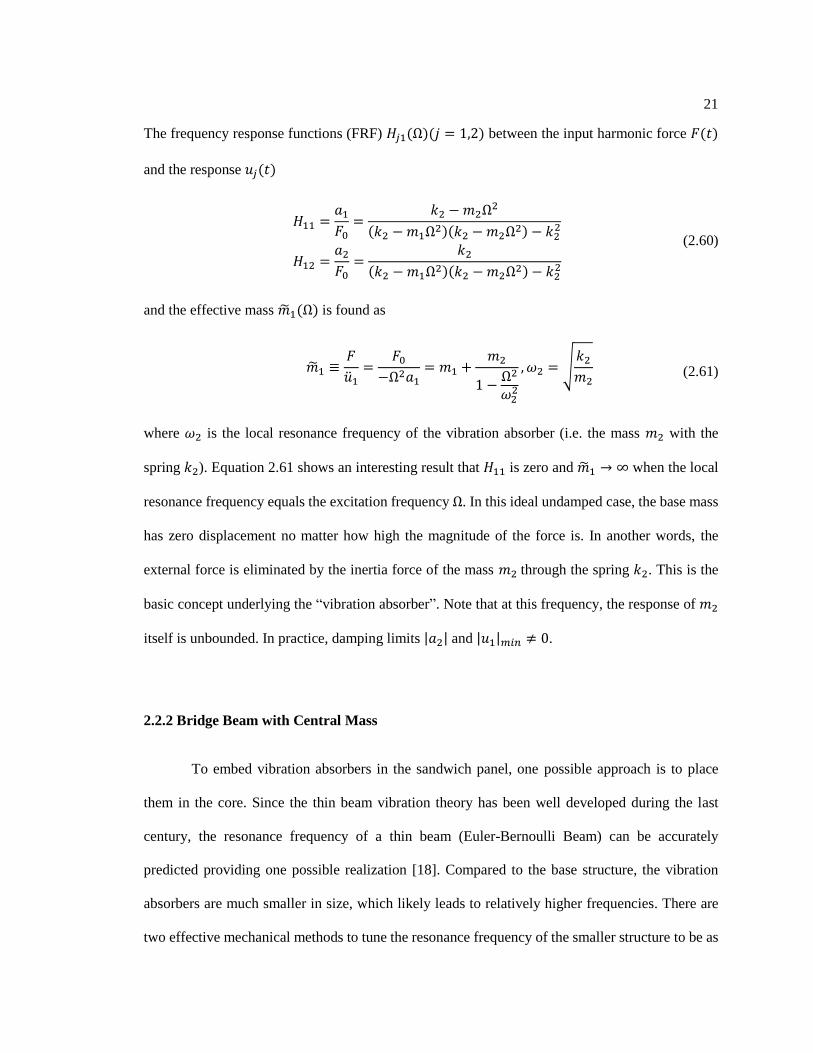
The frequency response functions (FRF) 𝐻𝑗1(Ω)(𝑗 = 1,2) between the input harmonic force 𝐹(𝑡)
and the response 𝑢𝑗(𝑡)
𝐻11 =𝑎1𝐹0=
𝑘2 −𝑚2Ω2
(𝑘2 −𝑚1Ω2)(𝑘2 −𝑚2Ω
2) − 𝑘22
𝐻12 =𝑎2𝐹0=
𝑘2(𝑘2 −𝑚1Ω
2)(𝑘2 −𝑚2Ω2) − 𝑘2
2
(2.60)
and the effective mass �̃�1(Ω) is found as
�̃�1 ≡𝐹
�̈�1=
𝐹0−Ω2𝑎1
= 𝑚1 +𝑚2
1 −Ω2
𝜔22
, 𝜔2 = √𝑘2𝑚2
(2.61)
where 𝜔2 is the local resonance frequency of the vibration absorber (i.e. the mass 𝑚2 with the
spring 𝑘2). Equation 2.61 shows an interesting result that 𝐻11 is zero and �̃�1 → ∞ when the local
resonance frequency equals the excitation frequency Ω. In this ideal undamped case, the base mass
has zero displacement no matter how high the magnitude of the force is. In another words, the
external force is eliminated by the inertia force of the mass 𝑚2 through the spring 𝑘2. This is the
basic concept underlying the “vibration absorber”. Note that at this frequency, the response of 𝑚2
itself is unbounded. In practice, damping limits |𝑎2| and |𝑢1|𝑚𝑖𝑛 ≠ 0.
2.2.2 Bridge Beam with Central Mass
To embed vibration absorbers in the sandwich panel, one possible approach is to place
them in the core. Since the thin beam vibration theory has been well developed during the last
century, the resonance frequency of a thin beam (Euler-Bernoulli Beam) can be accurately
predicted providing one possible realization [18]. Compared to the base structure, the vibration
absorbers are much smaller in size, which likely leads to relatively higher frequencies. There are
two effective mechanical methods to tune the resonance frequency of the smaller structure to be as
Page 31
22
low as those of the larger structure, which are reducing the stiffness, and increasing mass. In this
thesis, both methods are utilized; a “bridge beam” structure with centered mass is proposed as the
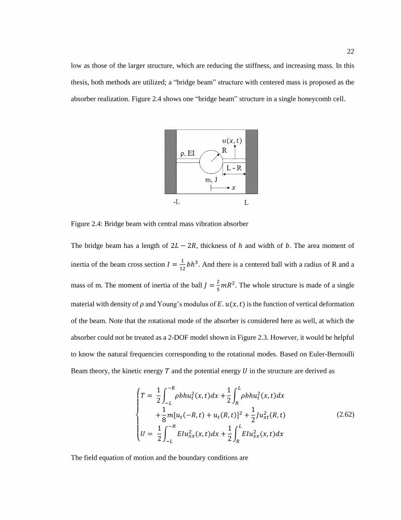
absorber realization. Figure 2.4 shows one “bridge beam” structure in a single honeycomb cell.
The bridge beam has a length of 2𝐿 − 2𝑅, thickness of ℎ and width of 𝑏. The area moment of
inertia of the beam cross section 𝐼 =1
12𝑏ℎ3. And there is a centered ball with a radius of R and a
mass of m. The moment of inertia of the ball 𝐽 =2
5𝑚𝑅2. The whole structure is made of a single
material with density of 𝜌 and Young’s modulus of 𝐸. 𝑢(𝑥, 𝑡) is the function of vertical deformation
of the beam. Note that the rotational mode of the absorber is considered here as well, at which the
absorber could not be treated as a 2-DOF model shown in Figure 2.3. However, it would be helpful
to know the natural frequencies corresponding to the rotational modes. Based on Euler-Bernoulli
Beam theory, the kinetic energy 𝑇 and the potential energy 𝑈 in the structure are derived as
{
𝑇 =
1
2∫ 𝜌𝑏ℎ𝑢𝑡
2(𝑥, 𝑡)𝑑𝑥 +−𝑅
−𝐿
1
2∫ 𝜌𝑏ℎ𝑢𝑡
2(𝑥, 𝑡)𝑑𝑥𝐿
𝑅
+1
8𝑚[𝑢𝑡(−𝑅, 𝑡) + 𝑢𝑡(𝑅, 𝑡)]
2 +1
2𝐽𝑢𝑥𝑡
2 (𝑅, 𝑡)
𝑈 =1
2∫ 𝐸𝐼𝑢𝑥𝑥
2 (𝑥, 𝑡)𝑑𝑥 +1
2∫ 𝐸𝐼𝑢𝑥𝑥
2 (𝑥, 𝑡)𝑑𝑥𝐿
𝑅
−𝑅
−𝐿
(2.62)
The field equation of motion and the boundary conditions are
Figure 2.4: Bridge beam with central mass vibration absorber
Page 32
23
𝜌𝑏ℎ𝑢𝑡𝑡(𝑥, 𝑡) + 𝐸𝐼𝑢𝑥𝑥𝑥𝑥(𝑥, 𝑡) = 0, ∀𝑥 ∈ (−𝐿,−𝑅) ∪ (𝑅, 𝐿)
𝑢(−𝐿, 𝑡) = 0∗, 𝑢(𝐿, 𝑡) = 0∗
𝑢𝑥(−𝑅, 𝑡) − 𝑢𝑥(𝑅, 𝑡) = 0∗, 𝑢(𝑅, 𝑡) − 𝑢(−𝑅, 𝑡) − 2𝑅𝑢𝑥(𝑅, 𝑡) = 0
∗
𝑢𝑥(−𝐿, 𝑡) = 0∗, 𝑢𝑥(𝐿, 𝑡) = 0
∗
1
2𝑚[𝑢𝑡𝑡(−𝑅, 𝑡) + 𝑢𝑡𝑡(𝑅, 𝑡)] + 𝐸𝐼[𝑢𝑥𝑥𝑥(𝑅, 𝑡) − 𝑢𝑥𝑥𝑥(−𝑅, 𝑡)] = 0
𝐽𝑢𝑥𝑡𝑡(𝑅, 𝑡) + 𝐸𝐼{𝑅[𝑢𝑥𝑥𝑥(𝑑, 𝑡) + 𝑢𝑥𝑥𝑥(−𝑅, 𝑡)] + 𝑢𝑥𝑥(−𝑅, 𝑡) − 𝑢𝑥𝑥(𝑅, 𝑡)} = 0
(2.63)
where the geometric boundary conditions are labeled with a “*”.
The geometric boundary conditions are fairly complicated on their own, hence the
development of a good set of assumed modes is difficult. However, the Finite Element Method
(FEM) can be used to model the absorber. A set of cubic interpolation shape functions are used to
approximate the transverse motion of a beam element.
𝑢(𝑒)(𝜉) = [1 − 3𝜉2 + 2𝜉3, 𝜉 − 2𝜉2 + 𝜉3, 3𝜉2 − 2𝜉3, −𝜉2 + 𝜉3] [
𝑢1𝑢2𝑢3𝑢4
]
(𝑒)
𝑤ℎ𝑒𝑟𝑒 𝜉 ∈ [0,1]
(2.64)
𝑢(𝑒)(0) = 𝑢1
(𝑒), 𝑢(𝑒)(1) = 𝑢3
(𝑒)
𝑢𝜉(𝑒)(0) = 𝑢2
(𝑒), 𝑢𝜉(𝑒)(1) = 𝑢4
(𝑒) (2.65)
where the superscript (𝑒) refers to the element number, and the subscript 𝜉 refers to the derivative
with respect to 𝜉. Equation 2.65 gives a result that 𝑢1(𝑒)
and 𝑢2(𝑒)
represent the displacement and
slope of the left node, while 𝑢3(𝑒)
and 𝑢4(𝑒)
represent the displacement and slope of the right node.
A few steps of derivation give the stiffness matrix and the mass matrix for a single element.
Page 33
24
[𝐾](𝑒) =(𝐸𝐼)(𝑒)
(𝐿(𝑒))3[
12 6 −12 66 4 −6 2−126
−62
12−6
−64
]
[𝑀](𝑒) = 𝜌(𝑒)𝐿(𝑒) [
13/35 11/210 9/70 −13/42011/210 1/105 13/420 −1/2109/70
−13/42013/420−1/140
13/35−11/210
−11/2101/105
]
(2.66)
where 𝐿(𝑒) is the length of the element, (𝐸𝐼)(𝑒) is the product of the Young’s modulus and the area
moment of inertia, and 𝜌(𝑒) is the density per unit length of the element. The next step is to
assemble the element matrices into global matrices. If there are 2𝑁 elements in the model, the total
number of nodes is 2𝑁 + 2, and the global mass matrix [𝑀] would be a (4𝑁 + 4) × (4𝑁 + 4)
matrix
[𝑀] =
[ 𝑀11
(1)𝑀12(1)
𝑀13(1)
𝑀14(1)
𝑀21(1)
𝑀22(1)
𝑀23(1)
𝑀24(1)
𝑀31(1)
𝑀32(1)
𝑀33(1)+𝑀11
(2)𝑀34(1)+𝑀12
(2)𝑀13(2)
𝑀14(2)
𝑀41(1)
𝑀42(1)
𝑀43(1)+𝑀21
(2)
𝑀31(2)
𝑀41(2)
𝑀44(1)+𝑀22
(2)𝑀23(2)
𝑀24(2)
𝑀32(2)
𝑀33(2)+𝑀11
(3)𝑀34(2)+𝑀12
(3)
𝑀42(2)
𝑀43(2)+𝑀21
(3)𝑀44(2)+𝑀22
(3)
⋯ 0
⋮ ⋱ ⋮0 ⋯ ]
(2.67)
The assembly procedure is also applicable to the global stiffness matrix [𝐾]. The next step
is to address the boundary condition. The mass of the ball 𝑚 is added to the term [𝑀]𝑁,𝑁 since
[𝑀]𝑁,𝑁 represents the mass of the center node. And the moment of inertia of the ball 𝐽 is added to
the term [𝑀]𝑁+1,𝑁+1 since [𝑀]𝑁+1,𝑁+1 represents the inertia of the center node. Then eliminating
the first two rows and columns, and the last two rows and columns for both matrices reflects the
cantilevered boundary conditions for both ends of the beam. Now the size of the global matrices is
4𝑁 × 4𝑁.
Page 34
25
With the global stiffness and mass matrices determined, the resonance frequencies of the
vibration absorbers can be found by solving the same eigenvalue problems described by Equation
2.50.
2.2.3 Distributed Tuned Mass Absorbers
Zapfe and Lesieutre presented a model for the application of highly distributed tuned mass
absorbers to a beam [19]. In the frequency domain, let 𝑠 = 𝑖Ω, the “effective mass” of the absorbers
can be expressed as
𝑀𝑒𝑓𝑓(𝑠) =∑𝑚𝑗
(𝑚𝑗𝑘𝑗) 𝑠2 + 1
𝑁
𝑗=1
(2.68)
where 𝑘𝑗 and 𝑚𝑗 are the stiffness and mass of the 𝑗th absorber. Note that if the resonance frequency
of the absorber 𝜔𝑗 = √𝑘𝑗
𝑚𝑗≫ the forcing frequency Ω, the denominator of the right hand side of
Equation 2.68 is almost 1, thus the effective mass is simply the summation of the mass of N
absorbers. If Ω ≫ 𝜔𝑗, the denominator of the right hand side will be much larger than one, which
means that the masses are effectively motionless, and the system behaves like N parallel springs.
Damping in the springs can be modeled by replacing the stiffness of the absorber by a complex
quantity, giving
𝑘𝑗∗ = 𝑘𝑗(1 + 𝑖𝜂𝑗) (2.69)
where 𝜂𝑗 is the loss factor of the spring material.
Substituting Equation 2.69 into Equation 2.68 provides the frequency-dependent effective
mass for a collection of inertial absorbers
Page 35
26
𝑀𝑒𝑓𝑓(𝑖Ω) =∑𝑚𝑗𝜔𝑗
2(1 + 𝑖𝜂𝑗)
𝜔𝑗2(1 + 𝑖𝜂𝑗) − Ω
2
𝑁
𝑗=1
(2.70)
Evidently, the effective mass would be a complex quantity. In this thesis, all the absorbers
are considered to be the same and are uniformly distributed, so Equation 2.70 can be rewritten in
terms of effective mass per unit volume, or effective density
𝜌𝑒𝑓𝑓(Ω) =𝑀𝑒𝑓𝑓(Ω)
𝑎𝑏ℎ=
𝑁
𝑎𝑏ℎ
𝑚𝜔2(1 + 𝑖𝜂)
𝜔2(1 + 𝑖𝜂) − Ω2 (2.71)
where 𝑎 and 𝑏 are the length and width of the sandwich panel, and ℎ is the thickness of the
honeycomb core. Then inserting the complex effective mass of the absorbers into the mass matrix
as developed in Section 2.1.3 yields a complex mass matrix that is a function of the forcing
frequency Ω
[𝑀]𝑟𝑠𝑟′𝑠′(Ω) = {{2𝜌𝑝𝑙𝑦𝑡 + [𝜌𝑐𝑜𝑟𝑒 + 𝜌𝑒𝑓𝑓(Ω)]ℎ}𝑎𝑏
(𝑟 + 𝑟′ + 3)(𝑠 + 𝑠′ − 1)(1
2)𝑠+𝑠′−2
𝑠 + 𝑠′ 𝑒𝑣𝑒𝑛
0 𝑠 + 𝑠′ 𝑜𝑑𝑑
(2.72)
Following the same procedure developed in Section 2.1.7, the frequency response function
from an input force to an output displacement is readily found.
2.3 Summary
In this chapter, an assumed modes model was developed based on Euler-Bernoulli Beam
theory for analyzing the dynamic behaviors of the perfect cantilevered plate and the “spring-
pinned” plate. Solving the eigenvalue problem shown in Equation 2.50 yields the analytical modal
frequencies and mode shapes of a plate, which will be used in Chapter 4. The frequency response
function shown in Equation 2.57 will be used for evaluating the elastic properties of the cores and
Page 36
27
predicting the frequency response in the vibration test for the cores and the sandwich panels in
Chapter 3.
The Finite Element Method was used to study the natural frequencies and mode shapes of
the vibration absorbers. The vibration absorbers were included in the plate model by treating them
as a complex effective density, which is a function of the excitation frequency. Inserting the
effective density into the mass matrix of the assumed modes model yields a complex mass matrix
shown in Equation 2.72. The updated EOM with the complex mass matrix will be used for
predicting the frequency responses of the core and the sandwich panel with the vibration absorbers
system.
Equation Chapter (Next) Section 1
Page 37
28
Chapter 3
Prototype Fabrication and Model Prediction
3.1 Design of the Specimens
With the model developed in Chapter 2, the size and mechanical properties of the sandwich
panel prototypes, and their parts (honeycomb cores, vibration absorbers system and face sheets)
can be determined. Two prototypes were designed: one used the baseline honeycomb core, and the
other one used the same honeycomb core with the addition of the vibration absorber system.
3.1.1 Honeycomb Core
Honeycomb cores are commonly used in sandwich composites for their light weight and
quasi-isotropic mechanical properties. The original idea for the design is to tune the first modal
frequency of both the sandwich panels and the vibration absorbers into 500 Hz. The size of the
sandwich panel was prescribed as 200 mm × 100 mm. So a design of the baseline honeycomb core
is given as shown in Figure 3.1. The size of each single cell is large enough to accommodate a
bridge beam absorber, which ideally has a first modal frequency of 500 Hz. The core consists seven
rows, each of which includes 11 or 12 hexagon cells. The side length of the centerline of the cell is
10 mm, the height of the cell is 20 mm, and the thickness of the wall is 1 mm.
Page 38
29
3.1.2 Vibration Absorber
As discussed in Section 2.2.2, the “bridge-beam” structures with center mass are being
used as the absorbers to reduce the vibration response. Figure 3.2 shows the honeycomb core with
the vibration absorbers, which are highly distributed in the core -- each cell contains one absorber.
The radius of the central ball is 4.42 mm, the width and thickness of the beam are 1 mm and 2 mm
respectively, and the length of the whole “bridge” is 18.84 mm. Note that the orientations of two
adjacent absorbers in the same row are always different, which makes the absorbers system quasi-
isotropic. It was found in the later experiment that the natural frequencies for the absorbers was
lower than predicted because of the inaccuracy of the model. Meanwhile, the natural frequencies
of the cantilevered sandwich panel were also lower than predicted, because the poor
implementation of the cantilevered boundary condition decreased the stiffness of the structure,
Figure 3.1: The baseline honeycomb core without absorbers (units in mm)
Page 39
30
hence reduced the natural frequencies. Therefore, the frequencies of the global structure and those
of the local structure still match fairly well, though there are certain biases.
3.1.3 Face Sheets
Both isotropic and anisotropic materials could be candidates for the face sheets. However,
to minimize the weight of the face sheets, a unidirectional carbon fiber composite, which is very
stiff in the X direction and much less stiff in the Y direction, is most suitable. Table 3.1 shows the
mechanical properties of the unidirectional carbon fiber used in this research, which was provided
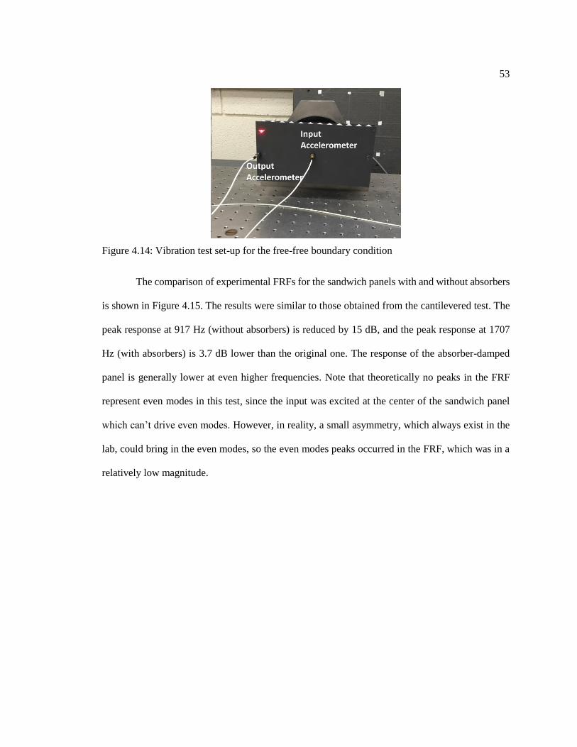
by ACP Composites, Inc [20].
Figure 3.2: Design drawing of the honeycomb core with metamaterial absorbers (units in mm)
Page 40
31
3.2 Manufacturing of Honeycomb Cores
Based on the solidwork drawing shown in Figure 3.1 and 3.2, two honeycomb cores were
manufactured using 3-D printing technology. Figure 3.3 (a) shows the printer used in the research,
the Objet 260 Connex 3-D printer, which is able to print using two different materials (usually one
stiff, and the other soft) simultaneously.
Figure 3.3 (b) shows the printed honeycomb cores; B is the baseline core and A is the one
with absorber system. Table 3.2 provides the material properties of the polymers that comprise the
Table 3.1: Mechanical properties of unidirectional carbon fiber plate
Property Density Young’s
Modulus 0˚
Young’s
Modulus 90˚
In-plane Shear
Modulus
Major Poisson’s
Ratio
Value 1.6 g/cm3 135 GPa 10 GPa 5 GPa 0.3
Figure 3.3: (a)Objet 260 Connex 3-D printer and (b)3-D printed honeycomb cores with and without
absorber system
Page 41
32
core. Both DM 8510 and DM 9860 are mixtures of two materials, TangoBlackPlus and VeroWhite,
which are commercial digital materials developed based on Objet PolyJetTM Technology. DM 8510
is the white material, rigid and ABS-like, consisting of more VeroWhite, while DM 9860 is the
black material, flexible and rubber-like, consisting of more TangoBlackPlus.
The data sheet for PolyJetTM materials provides the hardness of DM 9860, but does not
give the Young’s modulus. The Young’s modulus of DM 9860 is calculated from the empirical
formula for elastomers derived by Gent [21]
𝐸 = 0.0981(56 + 7.62336𝑆)
0.137505(254 − 2.54𝑆) (3.1)
where 𝐸 is the Young’s modulus in MPa and 𝑆 is the Shore A hardness.
3.3 Model Prediction
3.3.1 Natural frequencies of Absorbers
With the knowledge of the parameters, the FEM model developed in Section 2.2.2 was
coded in MATLAB, and the first 4 natural frequencies and their corresponding mode shapes are
shown in Figure 3.4. The detail of the code is in Appendix Section 2.
Table 3.2: Material Properties of the honeycomb core and vibration absorbers [22]
Properties Honeycomb
Core
Vibration
Absorbers
Material name DM 8510 DM 9860
Hardness (Shore A) N/A 60
Young’s modulus (MPa) 2350 3.605
Density (g/cm3) 1.16 1.13
Total mass (g) 63.35 35.84
Page 42
33
ANSYS was also used for modal analysis of the vibration absorber [23]. 10-Node
tetrahedral structural solid elements were used to mesh the structure. Figure 3.5 shows the first 4
modal frequencies in transverse motion and their corresponding mode shapes. Other in-plane
modes and twisting modes also exist, but are not shown here since they are irrelevant to the
reduction of transverse vibration of the sandwich panel. The transverse movement of the ball is
most significant in the first mode shape. The ball is rotating or not moving much in the other mode
shapes. Therefore, the absorber system would likely be most effective in reducing transverse
vibration around the frequency of 84.52 Hz. The effective density of the absorber system in
Equation 2.71 is distributed in a somewhat ad hoc method as shown in Equation 3.2:
Figure 3.4: Modal frequencies and corresponding mode shapes of the vibration absorber given by
the FEM model using 400 elements
0 0.002 0.004 0.006 0.008 0.01 0.012 0.014 0.016 0.018-1
-0.8
-0.6
-0.4
-0.2
0
0.2
0.4
0.6
0.8
1Vibration Absorber FEM 400 Elements Mode Shapes
x
W
Mode 1 95.09Hz
Mode 2 306.55Hz
Mode 3 2709.64Hz
Mode 4 2819.19Hz
Page 43
34
𝜌𝑒𝑓𝑓 = ∑𝑟𝑛𝜌𝑒𝑓𝑓
4
𝑛=1
(𝜔𝑛) (3.2)
where 𝑛 is the mode number, 𝜔𝑛 is the natural frequency of the 𝑛th mode, and 𝑟𝑛 is a distribution
factor: 𝑟1 = 7/10, 𝑟2 = 1/10, 𝑟3 = 1/5, 𝑟4 = 0, so that ∑ 𝑟𝑛4𝑛=1 = 1. The 2nd and 4th modes of the
absorber are rotational modes, which should be treated as an effective inertia in the global plate
model. The thin plate assumption is used for the global plate model in which only lateral motion is
considered, so 𝑟2 and 𝑟4 should be zero in this model. However, there are some damping effects
observed in the experimental data brought by the rotational modes of the absorbers, albeit small
ones. To describe the damping effects in this effective mass model, 𝑟2 is assigned as a non-zero
small number.
Figure 3.5: Modal frequencies and corresponding mode shapes of the vibration absorber given by
ANSYS
Page 44
35
Note that the modal frequencies from ANSYS are lower than the ones from MATLAB,
especially for the higher modes, as shown in Table 3.3. The main reason is because shear
deformation, which is not negligible for higher modes, is included in the ANSYS analysis, but not
in the model in MATLAB. The ANSYS results would be used in the following chapters, since it is
more accurate.
3.3.2 Frequency Response of Sandwich Panel
The model developed in Chapter 2 yields frequency response functions for a perfectly
cantilevered sandwich panel with the face sheet thickness varying from 0.014 inch to 0.034 inch,
as shown in Figure 3.6. The loss factor of the absorbers is prescribed as a typical number, 0.5. The
first two peak responses are reduced by the absorbers for all different thicknesses. Three thicknesses
were available from ACP, 0.014 inch, 0.022 inch and 0.03 inch. In the first glance, 0.014 inch might
be the best choice for the largest reduction of the first peak response. However, considering the
reality that the cantilevered boundary condition could never be perfect, which makes the natural
frequency of the sandwich panel lower than predicted, a thickness of 0.03 inch was chosen to
counteract the expected bias of the model.
Table 3.3: Comparison of modal frequencies prediction of the vibration absorber between
MATLAB and ANSYS
Modal
number MATLAB ANSYS Mode shape
1 95.09 Hz 84.52 Hz Translation
2 306.55 Hz 194.28 Hz Rotation
3 2709.64 Hz 1981.2 Hz Translation
4 2819.19 Hz 2032.3 Hz Rotation
Page 45
36
3.4 Sandwich Panel Fabrication
Two pieces of 0.03-inch-thick unidirectional carbon fiber face sheets were bonded to each
side of both the baseline core and the core with absorber system. The adhesive used here was 3MTM
Scotch-WeldTM Epoxy DP 190 Translucent, which has an overlap shear strength of 800 psi on an
aluminum surface after curing for 24 hours, according to the technical data sheet [24]. To decrease
the potential damping added by the adhesive, the adhesive film was smeared on the surface of the
face sheet as thinly as possible. Face sheets were bonded to one side of both cores first and, after 3
days for curing, face sheets were bonded to the other sides as well. The upper two pictures in Figure
3.7 show the cores with face sheets bond on one side, and the lower two pictures shows the finished
sandwich panels.
Figure 3.6: Prediction of frequency response function for the perfect cantilevered sandwich panel
with unidirectional carbon fiber face sheets of various thicknesses
102
103
104
-150
-100
-50
0
50
|Mag| (d
B)
Frequency (Hz)
Face Sheet Thickness 0.014 inch
With absorber
Without absorber
102
103
104
-150
-100
-50
0
50
|Mag| (d
B)
Frequency (Hz)
Face Sheet Thickness 0.018 inch
With absorber
Without absorber
102
103
104
-150
-100
-50
0
50
|Mag| (d
B)
Frequency (Hz)
Face Sheet Thickness 0.022 inch
With absorber
Without absorber
102
103
104
-150
-100
-50
0
50
|Mag| (d
B)
Frequency (Hz)
Face Sheet Thickness 0.026 inch
With absorber
Without absorber
102
103
104
-150
-100
-50
0
50
|Mag| (d
B)
Frequency (Hz)
Face Sheet Thickness 0.03 inch
102
103
104
-150
-100
-50
0
50
|Mag| (d
B)
Frequency (Hz)
Face Sheet Thickness 0.034 inch
With absorber
Without absorber
With absorber
Without absorber
Page 46
37
Equation Chapter (Next) Section 1
Figure 3.7: Finishing sandwich panels: Honeycomb cores bonded with unidirectional carbon fiber
face sheets
Page 47
38
Chapter 4
Experiment and Results
Experiments are essential to evaluate and to validate the vibration reduction effectiveness
of the absorber system. The chapter describes a static test that was used to evaluate the effective
elastic properties of the cores, and then addresses a vibration test that was used to determine the
natural frequencies of the cores for validating the accuracy of the model. Next, the vibration
experiments for the sandwich panels under various boundary conditions are presented, explaining
how data was obtained and analyzed to generate experimental FRFs. The previously determined
elastic properties were used in the model developed in Chapter 2 to generate simulation results.
Finally, the experimental FRFs and the simulated FRFs are compared.
4.1 Evaluating Elastic Properties
In Chapter 2, the meta-material absorbers are modeled as an effective added distributed
complex mass. Similarly, the honeycomb core could be considered as an isotropic plate with
effective Young’s modulus and Poisson’s ratio. The wall of the honeycomb core is fairly thick, so
the deflection from the shear deformation is neglected here. This section describes the static tests
used to evaluate the effective elastic properties of the core. To validate the isotropic plate model,
dynamic tests for the core were then conducted to provide the frequency response functions (FRFs),
which were compared with the numerical FRFs derived from the model.
Page 48
39
4.1.1 Effective Elastic Properties of the Core
Recalling the direct frequency response in Section 2.1.7, Equation 2.57 also holds for the
static case, in which the mass matrix term could be eliminated. So Equation 2.57 becomes
𝑤(𝑥0, 𝑦0) = {𝜙(𝑥0, 𝑦0)}
𝑇{𝑞∗}
= {𝜙(𝑥0, 𝑦0)}𝑇[𝐾]−1{𝜙(𝜉, 𝜂)}𝑢
(4.1)
where (𝑥0, 𝑦0) is the output location, and 𝑤 is the output displacement. (𝜉, 𝜂) is the input location,
and 𝑢 is the magnitude of the input force. Dividing 𝑢 in each side of Equation 4.1 yields
𝑤
𝑢= {𝜙(𝑥0, 𝑦0)}
𝑇[𝐾]−1{𝜙(𝜉, 𝜂)} (4.2)
For an isotropic plate, [𝐾] is a function of Young’s modulus and Poisson’s ratio. Therefore, solving
the least squares problem
minimize𝐸,𝜈
𝑓(𝐸, 𝜈) =1
𝑁√∑[(
𝑤
𝑢)𝑒− (
𝑤
𝑢)𝑎]2
𝑁
(4.3)
is a way to establish the effective Young’s modulus 𝐸 and effective Poisson’s ratio 𝜈. The subscript
𝑒 represents the experimental value, and 𝑎 represents the analytical value, while 𝑁 is the size of the
data set.
Based on Equation 4.3, a static test was set up as shown in Figure 4.1. The core was
cantilevered off the test table. A weight was hung from the core, serving as a vertical load, and a
linear variable differentiable transformer (LVDT) measured the transverse displacement of the
core. In total, 40 set of data were collected for 4 different applied load locations and 10 different
LVDT measurement locations. Figure 4.2 shows an example of data analysis in the location A1; a
straight line was fit from the set of force and displacement data, and the slope 0.4007 (mm/N) was
the experimentally-established value of 𝑤
𝑢.
Page 49
40
Using the data listed in Table 4.1, the effective Young’s modulus and Poisson’s ratio of
the honeycomb core were found to be: 𝐸𝑒𝑓𝑓 = 18.84𝑀𝑃𝑎, and 𝜐𝑒𝑓𝑓 = 0.322. The MATLAB code
for evaluating 𝐸𝑒𝑓𝑓 and 𝜐𝑒𝑓𝑓 is shown in Appendix Section 3. Substituting 𝐸𝑒𝑓𝑓 and 𝜐𝑒𝑓𝑓 back
into the model, the proportional errors of the analytical data are listed in Table 4.2. The arithmetic
mean of the error is 0.036 mm/N, which is fairly small relative to the majority of the data.
Figure 4.1: Static test set-up for the honeycomb core
Figure 4.2: Data analysis of static test in the location A1
y = 0.4007x - 0.0003
0
0.05
0.1
0.15
0.2
0.25
0.3
0.35
0.4
0.45
0 0 . 2 0 . 4 0 . 6 0 . 8 1 1 . 2
DIS
PLA
CEM
ENT(
MM
)
FORCE(N)
Page 50
41
4.1.2 Vibration Test for Cores
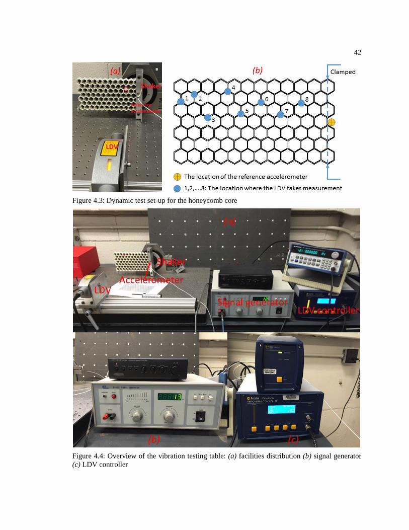
The vibration test was set up as shown in Figure 4.3 (a). The core was clamped and bolted
to the shaker, which was driven by a white noise signal during the test. An accelerometer was
attached at the center of the clamp to measure the input acceleration. And a Laser Doppler
Vibrometer (LDV) was used to measure the velocity of particular points on the core. The test was
repeated 8 times to collect data from different positions on the core as shown in Figure 4.3 (b). And
Figure 4.4 provides an overview of the test matrix for the vibration test.
Table 4.1: Experimental data of displacement divided by force in the static test (Unit: mm/N)
1 2 3 4 5 6 7 8 9 10
A 0.4007 0.4448 0.4009 0.1931 0.2519 0.0039 0.0755 0.0315 0.1473 0.324
B 0.5499 0.8985 0.627 0.2834 0.486 0.0015 0.0852 0.0477 0.2815 0.5971
C 0.0784 0.128 0.0686 0.0344 0.0706 0.0006 0.0172 0.0137 0.0541 0.0746
D 1.0878 0.6448 0.7989 0.4599 0.3493 0.0122 0.1786 0.0457 0.1389 0.5996
Table 4.2: Error (absolute value of [Experimental-Analytical]) of displacement divided by force in
the static test
1 2 3 4 5 6 7 8 9 10
A 0.031 0.015 0.011 0.039 0.019 0.001 0.031 0.002 0.020 0.021
B 0.130 0.129 0.014 0.063 0.024 0.001 0.060 0.000 0.002 0.014
C 0.052 0.020 0.057 0.042 0.028 0.000 0.020 0.003 0.016 0.042
D 0.172 0.083 0.045 0.020 0.080 0.008 0.017 0.004 0.091 0.011
Page 51
42
Figure 4.3: Dynamic test set-up for the honeycomb core
Figure 4.4: Overview of the vibration testing table: (a) facilities distribution (b) signal generator
(c) LDV controller
Page 52
43
A LabVIEW code named Modal Impact was used to collect the data. Figure 4.5 shows the
Graphical User Interface (GUI) of the “setup” code. The original data collected from each channel
were all time-domain data. The code transformed the time-domain data into frequency-domain
data, Auto Power Spectra, using a Fast Fourier Transformation (FFT). In a single test, data were
collected in 8 seconds, and repeated 20 times, using averaging to eliminate environmental noise.
The bandwidth was 0-800 Hz. Figure 4.6 shows the “current status” window during the test. The
upper screen shows the time domain data in each channel, while the lower screen shows the
averaged Auto Power Spectra for each channel.
Figure 4.5: GUI of Modal Impact, the LabVIEW code used to collect data
Page 53
44
Post-processing of the data was done by a MATLAB code associated with the Modal
Impact code. It generates a MATLAB figure plotting the frequency response functions (FRFs).
Figure 4.7 shows the comparison between the FRF for the core with absorbers and the FRF for the
baseline core at Location No. 2, near the free end, for which the frequency responses were clearest.
The output is the velocity measured by the LDV, while the input is the acceleration measured by
the accelerometer. Note that all the response peaks for the core with the absorber system were
reduced compared to those for the baseline core, which indicates the efficiency of the absorber
system in a broadband sense. For the excitation frequencies below or much higher than the absorber
resonance frequencies, the modal frequencies were lower for the core with absorber system,
because the absorber system adds mass to the structure which would reduce the frequencies. For
the excitation frequencies close to the absorber resonance frequencies, it is hard to tell whether the
mass effect, the absorber system behaves like distributed mass, or the stiffness effect, the absorber
system behaves like parallel springs, is more significant.
Figure 4.6: Status-checking window of the Modal Impact while collecting data
Page 54
45
Using the model developed in Chapter 2, modal frequencies and frequency responses were
also predicted. Figure 4.8 shows the model results for the modal frequencies and their
corresponding mode shapes.
Figure 4.7: Experimental frequency response comparison for two honeycomb cores alone
0 50 100 150 200 250 300 350 400 450 50010
1
102
103
104
105
106
Frequency (Hz)
Magnitude (
Outp
ut/
Input)
Frequency Response Function
Baseline Core
Core With Absorber
Absorber Resonance
Page 55
46
Figure 4.9 compares the predicted FRF to the experimental FRF. Various values of loss
factor, from 0.1 to 0.5, had been tried to compare the reduction of multiple peak responses acquired
Figure 4.8: Numerical results for honeycomb core without absorbers: first 6 modal frequencies and
their corresponding mode shapes
Figure 4.9: FRF comparison between experiment and simulation for the core with absorbers system
00.1
-0.05
0
0.05
-0.6
-0.4
-0.2
0
0.2
Frequency31.7944Hz
00.1
0.2-0.1
0
0.1
-5
0
5
x 10-4Frequency120.7325Hz
00.1
0.2-0.1
0
0.1
-0.04
-0.02
0
0.02
0.04
Frequency199.2551Hz
00.1
0.2
-0.1
-0.05
0
0.05
0.1
-2
0
2
x 10-4Frequency398.5897Hz
0
0.1
0.2
-0.1
0
0.1-1
0
1
2
x 10-3Frequency558.0847Hz
0
0.1
0.2
-0.1
0
0.1-1
0
1
2
3
x 10-4Frequency691.4536Hz
50 100 150 200 250 300 350 400 450 50010
2
103
104
105
106
Frequency (Hz)
Magnitude (
Outp
ut/
Input)
Frequency Response Function
Experiment
Simulation, loss factor = 0.3
Page 56
47
from the simulation to those acquired from the experiment. It is found that the usage of loss factor
𝜂 = 0.3 yields the peak responses reduction most close to those of the experiment. Meanwhile, the
model-predicted frequencies match the experiment very well in the range of 0-350 Hz. The
experimental FRF is lower than predicted over 350 Hz. One possible reason is that material
damping of the absorbers has greater impact for higher modes.
Table 4.3 lists and compares the modal frequencies obtained from the model and the
experiment. For the baseline core, the model predictions of the pure bending modal frequencies
were very accurate, with error less than 5%. But the prediction for other modes, such as a twisting
mode, had fairly large error. The two peaks in the experimental FRF between 200 Hz and 300 Hz
are not listed in Table 4.3, for these frequencies were confirmed as natural frequencies of the test
bed, which vibrated at large amplitude for input sine signals at these two frequencies.
In summary, the vibration test verified that the effective elastic properties gleaned from the
static test are accurate. And the assumed plate model is valid to analyze the vibration behavior of
the core for the lower modes, which suggests that the model would be also valid for analysis of the
sandwich panel.
Table 4.3: Comparison of model-predicted and experimentally-obtained natural frequencies for the
baseline core and the core with absorber
Modal
Number
Baseline Core Core with Absorber
Model Experiment Error Model Experiment Error
1 31.8 33.3 -4.50% 25 20.2 23.76%
2 120.7 77.8 55.14% 79 87.3 -9.51%
3 199.3 193.5 3.00% 115 117.2 -1.88%
4 398.6 419.0 4.87% 160 167.5 -4.48%
5 558.1 550.0 1.45% 419 375 11.74%
6 691.5 587.0 17.80%
Page 57
48
4.2 Vibration Tests of Sandwich Panels
Vibration tests were further conducted for the finished sandwich panels under various
boundary conditions. First, tests were done under a cantilevered boundary condition, excited by a
white noise signal impact to a shaker. The FRFs acquired from the experiments were compared
with the model-predicted FRFs. Finally, the test procedure was repeated under different free-free
boundary conditions. The experimental FRFs are discussed, although no accurate model prediction
was made. Table 4.4 shows the overall size and mass of the two sandwich panel specimens under
two boundary conditions.
4.2.1 Shaker-excited Cantilevered Sandwich Panel
The test was set up as shown in Figure 4.10. All the facilities used in the core testing were
also used in this test, and were arranged just as shown in Figure 4.4. Similarly, the sandwich panel
was clamped and bolted to the shaker, which a white noise signal to excite the root of the sandwich
panel. An accelerometer attached to the center of the clamp measured the input acceleration, while
another accelerometer attached at the tip of the panel measured the output acceleration. An LDV
Table 4.4: Overall size and mass of the sandwich panel specimens
Properties Sandwich panel
with baseline core
Sandwich panel with
vibration absorbers
Length in the cantilevered test
(mm) 156.69 156.69
Length in the free-free test
(mm) 208.85 208.85
Width (mm) 111.15 111.15
Thickness (mm) 21.52 21.52
Mass (g) 119.95 155.79
Effective density (g/cm3) 0.240 0.311
Page 58
49
system measured of the velocity at a corner of the panel. Figure 4.11 shows the parameter set-up
of the LabVIEW code. The channels collected time signal data for 5.12 seconds with a bandwidth
of 5000 Hz and the data were transformed into the frequency domain data using FFT software. The
process was repeated 40 times and the results averaged to eliminate environmental noise.
Figure 4.10: Vibration test set-up for cantilevered boundary condition
Page 59
50
The experimental FRFs were derived from the data collected by the two accelerometers,
and the magnitude was converted into dB.
𝑀𝑎𝑔 = 20log |𝑜𝑢𝑡𝑝𝑢𝑡
𝑖𝑛𝑝𝑢𝑡| (4.4)
Data taken with the LDV were very fuzzy in the high frequency range, so they were not used. Since
the clamp could not provide a perfect cantilevered boundary condition, the “spring-pinned” model
developed in Section 2.15 was used for analysis. The stiffness of the spring was prescribed as 3500
Nm to match the predicted first modal frequency with the experimentally-determined one.
The comparisons of the experimental FRFs and model FRFs for both sandwich panels are
shown in Figure 4.12 and Figure 4.13. The phases of the FRFs were “unwrapped” for clarity. The
four vertical dashed lines represent the four modal frequencies of the absorber system as shown in
Figure 3.5. For the sandwich panel without absorbers, the model matches the experiment very well
in the range from 200Hz to 2000Hz. On the model FRF, the reduction in peak response at the 355
Figure 4.11: LabVIEW set-up for vibration test of sandwich panels in the cantilevered boundary
condition
Page 60
51
Hz mode depends significantly on the value of 𝑟2 in Equation 3.2, which could be adjusted to match
the experimental result. On the experimental FRF, the two peaks lower than 200 Hz in the
experimental results likely represent resonance frequencies associated with the test table. For the
sandwich panel with absorbers, the peak responses near the natural frequencies of the meta-material
system are reduced; the peak response at 355Hz (without absorbers) is reduced by 15 dB, and the
peak response at 1835Hz (without absorbers) is separated into two peaks which are 7.3dB and
31.6dB lower than the original one. The absorber system is less effective at 1835 Hz, because 1835
Hz is close to the natural frequencies of two higher modes of the absorber, in which the center mass
is not moving very much. For frequencies higher than 2000Hz, no dramatic reduction was observed,
but the curve was much smoother, with almost no significant peaks.
Figure 4.12: Comparison of the FRFs acquired from (a) the experiment and (b) the model
102
103
-60
-40
-20
0
20
40
60
Frequency (Hz)
Magnitude (
dB
)
(a)
102
103
-60
-40
-20
0
20
40
60
Magnitude (
dB
)
Frequency (Hz)
(b)
Experiment No Absorber
Experiment With Absorber
Absorbers Resonance
Model With Absorber
Model No Absorber
Absorbers Resonance
15dB
31.6dB
7.3dB
11dB
Page 61
52
4.2.2 Shaker-excited Free-free Sandwich Panel
The vibration test was also conducted under free-free boundary conditions, although no
specific dynamic model was developed in the thesis; the polynomial assumed modes were not well
suited for use into free-free boundary condition. So the purpose of this test was to assess the
effectiveness of the metamaterial core in various frequency ranges. The back of the sandwich panel
was glued to a bolt which was screwed to the shaker as shown in Figure 4.14. The LabVIEW
parameters and the testing procedure were the same as those used for the cantilevered test.
Figure 4.13: Overall comparison of the FRFs acquired from the experiment and the model
102
103
-60
-40
-20
0
20
40
60
Frequency (Hz)
Magnitude (
dB
)
102
103
-2000
-1500
-1000
-500
0
500
Frequency (Hz)
Phase (
degre
e)
Experiment No Absorber
Experiment With Absorber
Model With Absorber
Model No Absorber
Absorbers Resonance
Page 62
53
The comparison of experimental FRFs for the sandwich panels with and without absorbers
is shown in Figure 4.15. The results were similar to those obtained from the cantilevered test. The
peak response at 917 Hz (without absorbers) is reduced by 15 dB, and the peak response at 1707
Hz (with absorbers) is 3.7 dB lower than the original one. The response of the absorber-damped
panel is generally lower at even higher frequencies. Note that theoretically no peaks in the FRF
represent even modes in this test, since the input was excited at the center of the sandwich panel
which can’t drive even modes. However, in reality, a small asymmetry, which always exist in the
lab, could bring in the even modes, so the even modes peaks occurred in the FRF, which was in a
relatively low magnitude.
Figure 4.14: Vibration test set-up for the free-free boundary condition
Page 63
54
Figure 4.15: Frequency response comparison for vibration test of sandwich panels in the free-free
boundary condition
102
103
-40
-20
0
20
40
Frequency(Hz)
Magnitude(d
B)
102
103
-1500
-1000
-500
0
500
Frequency(Hz)
Phase(d
egre
es)
Experiment No Absorber
Experiment With Absorber
Absorbers Resonance
3.7dB15dB
Page 64
55
Chapter 5
Conclusions and Future Work
5.1 Summary
This research addressed the design and demonstration of an acoustic meta-material
absorber system for reducing the dynamic response of, and noise transmission through, sandwich
panels in important frequency ranges. First, dynamic models for an absorber as well as for sandwich
panels with and without the absorber system were developed. Next, honeycomb cores with and
without the meta-material absorber system were manufactured using 3D printing, and characterized
statically and dynamically. Prototype sandwich panels were then manufactured according to a
design based on the dynamic model. Finally, vibration tests demonstrated that the meta-material
absorber system effectively reduces the vibration response at key design frequencies, typically by
3.7 - 15dB.
5.1.1 Dynamic Model for Metamaterial Absorber System
A polynomial assumed-modes plate model was presented to describe the motion of the
sandwich panel. Shear deformation and material damping are neglected in the model. A finite
element method implemented in MATLAB was used to predict the resonance frequency of the
vibration absorbers, and was validated by ANSYS results. In the plate dynamic model, the
absorbers are considered as a distributed complex mass which depends on the excitation frequency.
Page 65
56
5.1.2 Design and Manufacturing of the Specimen
The geometry and size of the honeycomb cores, absorbers, and face sheets were designed
with reference to the dynamic model. The cores for two sandwich panels were 3D-printed using a
stiff polymer for the baseline honeycomb core, and a combination of stiff and soft/lossy polymers
for the meta-material-augmented core. These cores were characterized statically to determine their
effective elastic properties, and then dynamically to determine the natural frequencies and loss
factors of the meta-material system. Unidirectional carbon-fiber face sheets were bonded on each
side of both cores to construct sandwich panels, which are the finished prototypes.
5.1.3 Experimental Test Validation
Vibration tests for the sandwich panel prototypes were conducted under two different
boundary conditions. For the cantilevered sandwich panel without absorbers, the model matches
the experiment very well in the frequencies range from 200Hz to 2000Hz. For the sandwich panel
with absorbers, the peak responses near the natural frequencies of the meta-material system were
reduced significantly. For the frequencies higher than 2000Hz, no dramatic reduction was observed,
but the curve was much smoother, with almost no discernable peaks.
For the other free-free boundary condition, the experimental FRF shows a similar trend,
namely that the peak responses near the local natural frequencies are reduced. In conclusion, the
experimental results demonstrated that the acoustic metamaterial core reduced the dynamic
response of the sandwich panels in the designed frequency range: 200 Hz - 2000 Hz, and offer
promise for broad band damping.
Page 66
57
5.2 Recommendations and Future Work
Two major research directions could evolve from the present work. The first one involves
improving the dynamic model, and the second, optimization of the design of the meta-material
absorber system.
5.2.1 Model Development
Since this work represents initial research on this topic, the dynamic model is appropriately
simplified. Material damping is not specifically included in the plate model, though it could be
significant, especially for higher modes. Meanwhile, the sandwich panel is rather thick compared
to the size, thus the Euler-Bernoulli plate assumption might not be accurate. Again for higher
modes, shear deformation could have a large impact on the prediction of modal frequencies. For
these reasons, material damping, shear deformation and potentially rotatory inertia should be added
to the plate model in the future.
The set of polynomial mode shape functions used works well for the cantilevered boundary
condition. But for the other boundary condition, such as free-free, it lacks accuracy. A FEM plate
model would be able to enhance the generality of the model.
The vibration absorbers are presently treated as distributed complex mass, a function of the
excitation frequency, in the dynamic model, and the effect of four absorber modes are considered
in an ad hoc manner. This treatment for the rotational modes of the vibration absorbers in particular
might not be accurate. They should be modeled as distributed effective inertia in the future work.
The effects of multiple absorber modes should be considered using an energy-based approach,
consistent with the assumed-modes method. Furthermore, the damping effects of all the absorbers
are considered to be identical. However, the efficiency of the absorbers might vary depending on
Page 67
58
their orientations and locations, and on the modes of the global structure. In addition, absorbers
could be tuned to different frequencies, and multiple modes of individual absorbers, including
rotational modes, might be effective at damping motions at different frequencies.
5.2.2 Specimen Design
The initial idea for the design was to tune the resonance frequencies of both the local and
global structures to roughly 500 Hz. But an early mistake in programming the MATLAB code
resulted in a initially a wrong prediction for the frequency of the absorbers (The real frequencies
are lower than predicted). This error was not found until the specimens had already been
manufactured. Fortunately, the poor cantilevered boundary condition in the lab reduced the
frequency of the global structure as well, so that the relative error was reduced. So it is useful for
future work to make a design that matches the global frequency or the excitation frequency to the
local frequency more precisely.
In the present work, the absorbers take on different orientations, which makes the absorber
system quasi-isotropic. However, the distribution is not optimized for the most efficient vibration
reduction. Nor is the geometry of the absorber optimized to have minimum weight. These two
perspectives are also promising for future study.
Finally, the absorbers could be tuned into different frequencies. As indicated by Zapfe and
Lesieutre [19], tuning the vibration absorber system over a range of design frequencies would be
helpful to broaden the effective damping band.
Page 68
59
Appendix
MATLAB Codes
1. Assumed Modes Model
1.1 Mode shapes of “spring-pinned” sandwich panels
1.1.1 Main program
%%%%%%%%%%%%%%%%%%%%%%%%%%%%%%%%%%%%%%%%%%%%%%%%%%%%%%%%%%%%%%%%%%%%%%%%%%
% This program solves the eigenvalue problem of the EOM for the
% spring-pinned sandwich panel, and plot the first 6 mode shapes and their
% corresponding natural frequencies.
% by Tianliang Yu
% Last Update May 2015
%%%%%%%%%%%%%%%%%%%%%%%%%%%%%%%%%%%%%%%%%%%%%%%%%%%%%%%%%%%%%%%%%%%%%%%%%%
clear;
global a b h Ec vc;
%a = 199.69e-3;
a = (199.69+4-47)*1e-3;
b = 111.15e-3;
h = 20e-3;
Ec = 18.836e6;
vc = 0.3219;
v12 = .3;
E1 = 135e9;
E2 = 10e9;
G12 = 5e9;
rhosheet = 1.6e3;
rhocore = 2.7291;
rhoB = 1.5437;
rhocore = rhocore + rhoB;
theta = [0;0];
R = 6; S = 6;
%Freq_test = 51.76;
t = 0.03*0.0254;
rhof = rhosheet*t;
rho = rhocore + rhof*2;
kappa = input('Stiffness of the spring = ? Pa');
[ K, M ] = StiffnessAndMassMatrix_spring( E1,E2,G12,v12,t,...
rho,theta,R,S,kappa);
[vv, dd] = eig(M\K);
wn = sort(abs(diag(dd)));
WN = sqrt(wn)/(2*pi);
x = 0:a/50:a;
Page 69
60
y = -b/2:b/20:b/2;
for k = 1:6
Phi = zeros(length(y),length(x));
rr = find(abs(diag(dd))==wn(k));
for r=1:R,
for s=1:S,
m = (r-1)*S + s;
for i = 1:length(x)
for j = 1:length(y)
temp = (x(i)/a)^(r+1)*(y(j)/b)^(s-1);
Phi(j,i) = Phi(j,i) + temp*vv(m,rr);
end
end
end
end
for i = 1:length(x)
for j = 1:length(y)
temp = x(i)/a;
Phi(j,i) = Phi(j,i) + temp*vv(R*S+1,rr);
end
end
figure(ceil(k/9));
if mod(k,6)==0
subplot(2,3,6);
else
subplot(2,3,mod(k,6));
end
surf(x,y,Phi);
title(['Frequency',num2str(WN(k)),'Hz']);
end
1.1.2 D matrix
function [ D ] = Dmatrix( E1,E2,G12,v12,t,theta)
% Dmatrix.m calculate the D matrix of the sandwich composite
% Tianliang Yu
global h Ec vc;
n = length(theta);% theta is a vector represents the plies angel of two
% face sheet in the squence starting from the bottom to the top
% Note: n must be an even number
D = zeros(3,3);
z = zeros(n+2,1);
Gc = Ec/(2*(1+vc)); % Ec, Gc and vc is the Young's modulus, shear stiffness
% and Poisson's ratio of the core
D = 1/3*Qbar(E1,E2,G12,v12,theta(1))*((-h/2)^3-(-h/2-t)^3)...
+1/3*Qbar(Ec,Ec,Gc,vc,0)*((h/2)^3-(-h/2)^3)...
+1/3*Qbar(E1,E2,G12,v12,theta(2))*((h/2+t)^3-(h/2)^3);
end
1.1.3 Q matrix
function [ Qbar ] = Qbar( E1,E2,G12,v12,theta )
% Qbar.m present Qbar matrix of for a given lamina engineering constants
Page 70
61
% Tianliang Yu
v21 = v12*E2/E1;%The Poisson's ratio for applying stress in the 2 direction
Q = zeros(3,3); %Initialize the matrix Q
Q(1,1) = E1/(1-v12*v21); %Q11
Q(1,2) = v12*E2/(1-v12*v21); %Q12
Q(2,1) = Q(1,2); %Q21=Q12
Q(2,2) = E2/(1-v12*v21); %Q22
Q(3,3) = G12; %2*Q66
T1 = Tstress(theta); %The tensor transformation matrix for stress
T2 = Tstrain(theta); %The tensor transformation matrix for strain
Qbar = T1\Q*T2;
end
function [ T ] = Tstrain( theta )
% Tmatrix.m present the tensor transformation matrix
% Tianliang Yu
T = zeros(3,3); %Initialize the matrix Q
T(1,1) = (cos(theta))^2; %T11
T(1,2) = (sin(theta))^2; %T12
T(1,3) = cos(theta)*sin(theta); %T13
T(2,1) = T(1,2); %T21=T12
T(2,2) = T(1,1); %T22=T11
T(2,3) = -cos(theta)*sin(theta); %T23
T(3,1) = -2*cos(theta)*sin(theta); %T31
T(3,2) = 2*cos(theta)*sin(theta); %T32
T(3,3) = (cos(theta))^2-(sin(theta))^2;%T33
end
function [ T ] = Tstress( theta )
% Tmatrix.m present the tensor transformation matrix
% Tianliang Yu
T = zeros(3,3); %Initialize the matrix Q
T(1,1) = (cos(theta))^2; %T11
T(1,2) = (sin(theta))^2; %T12
T(1,3) = 2*cos(theta)*sin(theta); %T13
T(2,1) = T(1,2); %T21=T12
T(2,2) = T(1,1); %T22=T11
T(2,3) = -2*cos(theta)*sin(theta); %T23
T(3,1) = -cos(theta)*sin(theta); %T31
T(3,2) = cos(theta)*sin(theta); %T32
T(3,3) = (cos(theta))^2-(sin(theta))^2;%T33
end
1.1.4 Stiffness and mass matrix
function [ K, M ] = StiffnessAndMassMatrix_spring( E1,E2,G12,...
v12,t,rho,theta,R,S,kappa )
% StiffnessMatrix_spring.m calculate the stiffness and mass matrix of the
% spring-pinned plate
% by Tianliang Yu
% Last updated 04/04/2014
global a b;
N = R*S;
K = zeros(N+1,N+1);
M = zeros(N+1,N+1);
D = Dmatrix( E1,E2,G12,v12,t,theta);
for r=1:R,
Page 71
62
for rp=1:R,
for s=1:S,
for sp=1:S,
I1 = (1/a^3*b*r*rp*((-1/2)^(s+sp)+(1/2)^(s+sp))...
*(r+1)*(rp+1)*2)/((r+rp-1)*(s+sp-1));
J = (a*b*((-1/2)^(s+sp)+(1/2)^(s+sp))*2)/(r+rp+3)/(s+sp-1);
if s < 2 || sp < 2
I2 = 0;
I3_1 = 0;
I3_2 = 0;
I3_3 = 0;
elseif s > 2 && sp > 2
I2 = (a/b^3*((-1/2)^(s+sp)+(1/2)^(s+sp))*(s-2)*...
(s-1)*(sp-2)*(sp-1)*32)/((r+rp+3)*(s+sp-5));
I3_1 = (r*((-1/2)^(s+sp)+(1/2)^(s+sp))*(r+1)*...
(sp*-3+sp^2+2)*8)/(a*b*(r+rp+1)*(s+sp-3));
I3_2 = (rp*((-1/2)^(s+sp)+(1/2)^(s+sp))*(rp+1)*...
(s*-3+s^2+2)*8)/(a*b*(r+rp+1)*(s+sp-3));
I3_3 = (2^(-s-sp)*((-1)^(s+sp)+1)*(r+1)*(rp+1)*...
(s-1)*(sp-1)*8)/(a*b*(r+rp+1)*(s+sp-3));
else
I2 = 0;
I3_1 = (r*((-1/2)^(s+sp)+(1/2)^(s+sp))*(r+1)*...
(sp*-3+sp^2+2)*8)/(a*b*(r+rp+1)*(s+sp-3));
I3_2 = (rp*((-1/2)^(s+sp)+(1/2)^(s+sp))*(rp+1)*...
(s*-3+s^2+2)*8)/(a*b*(r+rp+1)*(s+sp-3));
I3_3 = (2^(-s-sp)*((-1)^(s+sp)+1)*(r+1)*(rp+1)*...
(s-1)*(sp-1)*8)/(a*b*(r+rp+1)*(s+sp-3));
end
m = (r-1)*S + s;
n = (rp-1)*S + sp;
K(m,n) = D(1,1)*I1 + D(2,2)*I2 + D(1,2)*(I3_1+I3_2) + ...
4*D(3,3)*I3_3;
M(m,n) = rho*J;
end
end
end
end
K(N+1,N+1) = kappa*b/a^2;
% kappa is the stiffness of the spring
M(N+1,N+1) = 1/3*rho*a*b;
for r=1:R,
for s=1:S,
m = (r-1)*S + s;
if mod(s,2) == 2
M(m,N+1) = 0;
else
M(m,N+1) = rho*a*b/(s*(r+3))*(1/2)^(s-1);
end
M(N+1,m) = M(m,N+1);
end
end
Page 72
63
1.2 Frequency responses of “spring-pinned” sandwich panels
1.2.1 Main program
%%%%%%%%%%%%%%%%%%%%%%%%%%%%%%%%%%%%%%%%%%%%%%%%%%%%%%%%%%%%%%%%%%%%%%%%%%
% This program plot the frequency response functions of the "pinned-spring"
% sandwich panel with and without vibration absorber systems
% by Tianliang Yu
% Last Updated 05/07/2014
%%%%%%%%%%%%%%%%%%%%%%%%%%%%%%%%%%%%%%%%%%%%%%%%%%%%%%%%%%%%%%%%%%%%%%%%%%
clear;
global a b h Ec vc;
%a = 199.69e-3;
a = (199.69+4-47)*1e-3;
b = 111.15e-3;
h = 20e-3;
Ec = 18.836e6;
vc = 0.3219;
v12 = .3;
E1 = 135e9;
E2 = 10e9;
G12 = 5e9;
rhosheet = 1.6e3;
Thickness = 0.03*2.54e-2;
rhof = rhosheet*Thickness;
%kappa = 1e4;
theta = [0;0];
x0 = 0; y0 = 2e-3;
Pt = input('What is the output point number?');
if Pt == 0,
xi = a-9e-3; lambda = -4e-3;
elseif Pt == 1,
xi = 11/11.5*a; lambda = (3/11-1/2)*b;
elseif Pt == 2,
xi = 10/11.5*a; lambda = (9/11-1/2)*b;
elseif Pt == 3,
xi = 9/11.5*a; lambda = (6/11-1/2)*b;
elseif Pt == 4,
xi = 7.5/11.5*a; lambda = (9.5/11-1/2)*b;
elseif Pt == 5,
xi = 6.5/11.5*a; lambda = (6.5/11-1/2)*b;
elseif Pt == 6,
xi = 5/11.5*a; lambda = (8/11-1/2)*b;
elseif Pt == 7,
xi = 3.5/11.5*a; lambda = (6.5/11-1/2)*b;
elseif Pt == 8,
xi = 2/11.5*a; lambda = (8/11-1/2)*b;
end
rhocore = 2.7291;
rhoB = 1.5437;
%omega = 84.5198*2*pi;
omega = [84.5198; 194.283; 1981.2; 2032.33]*2*pi;
R = 6; S = 6;
%ratio = 10.2/0.02;
%eta = .3;
%%%%
Phi0 = VirtualWork(0,0,R,S);
Page 73
64
Phi1 = VirtualWork(x0,y0,R,S);
Phi2 = VirtualWork(xi,lambda,R,S);
Omega = logspace(1,4,1000);
Omega = Omega*2*pi;
I = sqrt(-1);
colors = ['r','b','g'];
figure();
kappa = 4e3;
for ii = 1:3
eta = 0.1 + ii*0.1;
for kk = 1:2
resp = zeros(length(Omega),1);
Theta = zeros(length(Omega),1);
for k = 1:length(Omega)
rho = rhocore + 2*rhof;
if kk == 1
for i = 1:length(omega)
if i == 1
rat = 7/10;
elseif i == 2
rat = 1/10;
elseif i == 3
rat = 1/5;
else
rat = 0;
end
rho = rho + rat*rhoB*omega(i)^2*(1+I*eta)/(omega(i)^2*...
(1+I*eta)-Omega(k)^2);
end
end
[K,M] = StiffnessAndMassMatrix_spring_basemotion( E1,E2,G12,v12,...
Thickness,rho,theta,R,S,kappa );
tip = Phi2'*(-(Omega(k))^2*M+K)^(-1)*Phi0;
base = Phi1'*(-(Omega(k))^2*M+K)^(-1)*Phi0;
resp(k) = tip/base;
Theta(k) = atan2(imag(resp(k)),real(resp(k)))*180/pi;
end
mag = abs(resp);
subplot(2,3,ii);
%loglog(Omega/(2*pi),mag,colors(kk)); hold on;
plot(Omega/(2*pi),20*log10(mag),colors(kk)); hold on;
xlabel('Frequency (Hz)');
xlim([0,5000])
subplot(2,3,ii+3);
%semilogx(Omega/(2*pi),Theta,colors(kk)); hold on;
plot(Omega/(2*pi),Theta,colors(kk)); hold on;
xlim([0,5000])
ylabel('Phase (degree)'); xlabel('Frequency (Hz)');
end
subplot(2,3,ii)
legend(['With absorber \eta = ',num2str(eta)],'Without absorber',...
'Location','NorthEast');
title(['Spring stiffness ',num2str(kappa),' Nm']);
end
Page 74
65
1.2.2 Stiffness and mass matrix
function [ K, M ] = StiffnessAndMassMatrix_spring_basemotion( E1,E2,G12,...
v12,t,rho,theta,R,S,kappa )
% StiffnessMatrix_spring_basemotion.m calculate the stiffness and mass
% matrix of the spring-pinned plate with the base motion mode
% by Tianliang Yu
% Last Updated 04/04/2014
global a b;
N = R*S;
K = zeros(N+2,N+2);
M = zeros(N+2,N+2);
D = Dmatrix( E1,E2,G12,v12,t,theta);
for r=1:R,
for rp=1:R,
for s=1:S,
for sp=1:S,
I1 = (1/a^3*b*r*rp*((-1/2)^(s+sp)+(1/2)^(s+sp))...
*(r+1)*(rp+1)*2)/((r+rp-1)*(s+sp-1));
J = (a*b*((-1/2)^(s+sp)+(1/2)^(s+sp))*2)/(r+rp+3)/(s+sp-1);
if s < 2 || sp < 2
I2 = 0;
I3_1 = 0;
I3_2 = 0;
I3_3 = 0;
elseif s > 2 && sp > 2
I2 = (a/b^3*((-1/2)^(s+sp)+(1/2)^(s+sp))*(s-2)*...
(s-1)*(sp-2)*(sp-1)*32)/((r+rp+3)*(s+sp-5));
I3_1 = (r*((-1/2)^(s+sp)+(1/2)^(s+sp))*(r+1)*...
(sp*-3+sp^2+2)*8)/(a*b*(r+rp+1)*(s+sp-3));
I3_2 = (rp*((-1/2)^(s+sp)+(1/2)^(s+sp))*(rp+1)*...
(s*-3+s^2+2)*8)/(a*b*(r+rp+1)*(s+sp-3));
I3_3 = (2^(-s-sp)*((-1)^(s+sp)+1)*(r+1)*(rp+1)*...
(s-1)*(sp-1)*8)/(a*b*(r+rp+1)*(s+sp-3));
else
I2 = 0;
I3_1 = (r*((-1/2)^(s+sp)+(1/2)^(s+sp))*(r+1)*...
(sp*-3+sp^2+2)*8)/(a*b*(r+rp+1)*(s+sp-3));
I3_2 = (rp*((-1/2)^(s+sp)+(1/2)^(s+sp))*(rp+1)*...
(s*-3+s^2+2)*8)/(a*b*(r+rp+1)*(s+sp-3));
I3_3 = (2^(-s-sp)*((-1)^(s+sp)+1)*(r+1)*(rp+1)*...
(s-1)*(sp-1)*8)/(a*b*(r+rp+1)*(s+sp-3));
end
m = (r-1)*S + s;
n = (rp-1)*S + sp;
K(m,n) = D(1,1)*I1 + D(2,2)*I2 + D(1,2)*(I3_1+I3_2) + ...
4*D(3,3)*I3_3;
M(m,n) = rho*J;
end
end
end
end
K(N+1,N+1) = kappa*b/a^2;
% kappa is the stiffness of the torsional spring
K(N+2,N+2) = k2/2;
% k2 is the stiffness of the transitional spring
M(N+1,N+1) = 1/3*rho*a*b;
M(N+1,N+2) = 1/2*rho*a*b;
M(N+2,N+1) = 1/2*rho*a*b;
Page 75
66
M(N+2,N+2) = rho*a*b;
for r=1:R,
for s=1:S,
m = (r-1)*S + s;
if mod(s,2) == 2
M(m,N+1) = 0;
M(m,N+2) = 0;
else
M(m,N+1) = rho*a*b/(s*(r+3))*(1/2)^(s-1);
M(m,N+2) = rho*a*b/(s*(r+2))*(1/2)^(s-1);
end
M(N+1,m) = M(m,N+1);
M(N+2,m) = M(m,N+2);
end
end
1.2.3 Virtual work
function [ Phi ] = VirtualWork( x,y,R,S )
% VirtualWork.m calculate the Virtual Work of the unit concentrated load
% applied on the cantilever plate
% Tianliang Yu
% Last Update 02/25/2015
global a b;
N = R*S;
Phi = zeros(N+2,1);
for r=1:R,
for s=1:S,
m = (r-1)*S + s;
Phi(m) = (x/a)^(r+1)*(y/b)^(s-1);
end
end
Phi(N+1) = x/a;
Phi(N+2) = 1;
end
1.3 Frequency responses of cantilevered sandwich panels
1.3.1 Main program
%%%%%%%%%%%%%%%%%%%%%%%%%%%%%%%%%%%%%%%%%%%%%%%%%%%%%%%%%%%%%%%%%%%%%%%%%%%
% This program plot the frequency response of cantilevered sandwich panels
% with unidirectional carbon fiber face sheets of various thicknesses
% by Tianliang Yu
% Last Updated 01/07/2015
%%%%%%%%%%%%%%%%%%%%%%%%%%%%%%%%%%%%%%%%%%%%%%%%%%%%%%%%%%%%%%%%%%%%%%%%%%%
clear;
global a b h Ec vc;
a = 199.69e-3;
b = 111.15e-3;
Page 76
67
h = 20e-3;
Ec = 18.836e6;
vc = 0.3219;
v12 = input('Poisson ratio = ');
E1 = input('E1 = ? GPa: ')*1e9;
E2 = input('E2 = ? GPa: ')*1e9;
G12 = input('G12 = ? GPa: ')*1e9;
rhosheet = input('Density = ? g/cm3: ')*1e3;
theta = [0;0];
x0 = 0; y0 = 1/2*b;
Pt = input('What is the output point number?');
if Pt == 1,
xi = 11/11.5*a; lambda = (3/11-1/2)*b;
elseif Pt == 2,
xi = 10/11.5*a; lambda = (9/11-1/2)*b;
elseif Pt == 3,
xi = 9/11.5*a; lambda = (6/11-1/2)*b;
elseif Pt == 4,
xi = 7.5/11.5*a; lambda = (9.5/11-1/2)*b;
elseif Pt == 5,
xi = 6.5/11.5*a; lambda = (6.5/11-1/2)*b;
elseif Pt == 6,
xi = 5/11.5*a; lambda = (8/11-1/2)*b;
elseif Pt == 7,
xi = 3.5/11.5*a; lambda = (6.5/11-1/2)*b;
elseif Pt == 8,
xi = 2/11.5*a; lambda = (8/11-1/2)*b;
end
rhocore = 2.7291;
rhoB = 1.5437;
omega = 511.45*2*pi;
R = 6; S = 6;
ratio = 10.2/0.02;
%%%%
Phi1 = VirtualWork(x0,y0,R,S);
Phi2 = VirtualWork(xi,lambda,R,S);
Omega = logspace(2,4,1000);
Omega = Omega*2*pi;
I = sqrt(-1);
colors = ['r','g','b'];
figure();
for ii = 1:6
Thickness = (0.018+ii*0.002)*2.54e-2;
rhof = rhosheet*Thickness;
for kk = 1:3
eta = 2*10^(-kk);
resp = zeros(length(Omega),1);
Theta = zeros(length(Omega),1);
for k = 1:length(Omega)
rho = rhocore + 2*rhof + rhoB*omega^2*(1+I*eta)/(omega^2*(1+I*eta)...
-Omega(k)^2);
[ K, M ] = StiffnessAndMassMatrix1( E1,E2,G12,v12,Thickness,rho,...
theta,R,S);
tip = Phi2'*(-(Omega(k))^2*M+K)^(-1)*Phi1;
base = Phi1'*(-(Omega(k))^2*M+K)^(-1)*Phi1;
resp(k) = tip/(base*Omega(k))*ratio;
Theta(k) = atan2(imag(resp(k)),real(resp(k)))*180/pi;
end
mag = abs(resp);
subplot(3,2,ii);
semilogx(Omega/(2*pi),20*log10(mag),colors(kk)); hold on;
Page 77
68
ylabel('|Mag| (dB)'); xlabel('Frequency (Hz)');
end
legend('\eta = 0.5','\eta = 0.05','\eta = 0.005','Location','NorthEast');
title(['Face Sheet Thickness ',num2str(Thickness/2.54e-2),' inch']);
end
1.3.2 Stiffness and mass matrix
function [ K, M ] = StiffnessAndMassMatrix1( E1,E2,G12,v12,t,rho,theta,R,S )
% StiffnessMatrix1.m calculate the stiffness and mass matrix of the
% cantilevered plate with the base motion mode
% by Tianliang Yu
% Last Updated 01/30/2014
global a b;
N = R*S;
K = zeros(N+1,N+1);
M = zeros(N+1,N+1);
D = Dmatrix( E1,E2,G12,v12,t,theta);
for r=1:R,
for rp=1:R,
for s=1:S,
for sp=1:S,
I1 = (1/a^3*b*r*rp*((-1/2)^(s+sp)+(1/2)^(s+sp))...
*(r+1)*(rp+1)*2)/((r+rp-1)*(s+sp-1));
J = (a*b*((-1/2)^(s+sp)+(1/2)^(s+sp))*2)/(r+rp+3)/(s+sp-1);
if s < 2 || sp < 2
I2 = 0;
I3_1 = 0;
I3_2 = 0;
I3_3 = 0;
elseif s > 2 && sp > 2
I2 = (a/b^3*((-1/2)^(s+sp)+(1/2)^(s+sp))*(s-2)*...
(s-1)*(sp-2)*(sp-1)*32)/((r+rp+3)*(s+sp-5));
I3_1 = (r*((-1/2)^(s+sp)+(1/2)^(s+sp))*(r+1)*...
(sp*-3+sp^2+2)*8)/(a*b*(r+rp+1)*(s+sp-3));
I3_2 = (rp*((-1/2)^(s+sp)+(1/2)^(s+sp))*(rp+1)*...
(s*-3+s^2+2)*8)/(a*b*(r+rp+1)*(s+sp-3));
I3_3 = (2^(-s-sp)*((-1)^(s+sp)+1)*(r+1)*(rp+1)*...
(s-1)*(sp-1)*8)/(a*b*(r+rp+1)*(s+sp-3));
else
I2 = 0;
I3_1 = (r*((-1/2)^(s+sp)+(1/2)^(s+sp))*(r+1)*...
(sp*-3+sp^2+2)*8)/(a*b*(r+rp+1)*(s+sp-3));
I3_2 = (rp*((-1/2)^(s+sp)+(1/2)^(s+sp))*(rp+1)*...
(s*-3+s^2+2)*8)/(a*b*(r+rp+1)*(s+sp-3));
I3_3 = (2^(-s-sp)*((-1)^(s+sp)+1)*(r+1)*(rp+1)*...
(s-1)*(sp-1)*8)/(a*b*(r+rp+1)*(s+sp-3));
end
m = (r-1)*S + s;
n = (rp-1)*S + sp;
K(m,n) = D(1,1)*I1 + D(2,2)*I2 + D(1,2)*(I3_1+I3_2) + ...
4*D(3,3)*I3_3;
M(m,n) = rho*J;
end
end
end
end
Page 78
69
for r=1:R,
for s=1:S,
m = (r-1)*S + s;
K(m,N+1) = 0;
if mod(s,2) == 2
M(m,N+1) = 0;
else
M(m,N+1) = rho*a*b/s*(r+2)*(1/2)^(s-1);
end
K(N+1,m) = K(m,N+1);
M(N+1,m) = M(m,N+1);
end
end
K(N+1,N+1) = 0;
M(N+1,N+1) = rho*a*b;
1.3.3 Virtual work
function [ Phi ] = VirtualWork( x,y,R,S )
% VirtualWork.m calculate the Virtual Work of the unit concentrated load
% applied on the cantilever plate
% Tianliang Yu
% 02/25/2015
global a b;
N = R*S;
Phi = zeros(N+1,1);
for r=1:R,
for s=1:S,
m = (r-1)*S + s;
Phi(m) = (x/a)^(r+1)*(y/b)^(s-1);
end
end
Phi(N+1) = 1;
end
1.4 Mode shapes of cantilevered cores
1.4.1 Main program
%%%%%%%%%%%%%%%%%%%%%%%%%%%%%%%%%%%%%%%%%%%%%%%%%%%%%%%%%%%%%%%%%%%%%%%%%%%
% This program solves the eigenvalue problem of the EOM for the
% cantilevered cores, and plot the first 6 mode shapes and their
% corresponding natural frequencies.
% by Tianliang Yu
% Last Updated 01/30/2014
%%%%%%%%%%%%%%%%%%%%%%%%%%%%%%%%%%%%%%%%%%%%%%%%%%%%%%%%%%%%%%%%%%%%%%%%%%%
clear;
global a b h;
a = 199.69e-3;
b = 111.15e-3;
Page 79
70
h = 20e-3;
E = 18.836e6;
v = 0.3219;
rhoA = 2.7291;
rhoB = 1.5437;
rhoA = rhoA + rhoB;
R = 6; S = 6;
%%%%%%%%%%%%%%%%%%%%%%%%%%%%%%%%%%%%%%%%%%%%%%%%%%%%%%%%%%%%%%%%%%%%%%%%%%%
[ K, M ] = StiffnessAndMassMatrix1( v,E,rhoA,R,S);
[vv, dd] = eig(M\K);
wn = sort(abs(diag(dd)));
WN = sqrt(wn)/(2*pi);
x = 0:a/50:a;
y = -b/2:b/20:b/2;
for k = 1:6
Phi = zeros(length(y),length(x));
[cc,rr] = find(abs(dd)==wn(k));
for r=1:R,
for s=1:S,
m = (r-1)*S + s;
for i = 1:length(x)
for j = 1:length(y)
temp = (x(i)/a)^(r+1)*(y(j)/b)^(s-1);
Phi(j,i) = Phi(j,i) + temp*vv(m,rr);
end
end
end
end
figure(ceil(k/6));
if mod(k,6)==0
subplot(2,3,6);
else
subplot(2,3,mod(k,6));
end
surf(x,y,Phi);
title(['Frequency',num2str(WN(k)),'Hz']);
end
1.4.2 Stiffness and mass matrix
function [ K, M ] = StiffnessAndMassMatrix1( v,E,rho,R,S )
% StiffnessMatrix1.m calculate the stiffness and mass matrix of the
% cantilevered cores
% by Tianliang Yu
% Last Updated 01/30/2015
global a b h;
N = R*S;
K = zeros(N,N);
M = zeros(N,N);
for r=1:R,
for rp=1:R,
for s=1:S,
for sp=1:S,
I1 = (1/a^3*b*r*rp*((-1/2)^(s+sp)+(1/2)^(s+sp))...
*(r+1)*(rp+1)*2)/((r+rp-1)*(s+sp-1));
J = (a*b*((-1/2)^(s+sp)+(1/2)^(s+sp))*2)/(r+rp+3)/(s+sp-1);
if s < 2 || sp < 2
Page 80
71
I2 = 0;
I3 = 0;
elseif s > 2 && sp > 2
I2 = (a/b^3*((-1/2)^(s+sp)+(1/2)^(s+sp))*(s-2)*...
(s-1)*(sp-2)*(sp-1)*32)/((r+rp+3)*(s+sp-5));
I3_1 = (r*v*((-1/2)^(s+sp)+(1/2)^(s+sp))*(r+1)*...
(sp*-3+sp^2+2)*8)/(a*b*(r+rp+1)*(s+sp-3));
I3_2 = (rp*v*((-1/2)^(s+sp)+(1/2)^(s+sp))*(rp+1)*...
(s*-3+s^2+2)*8)/(a*b*(r+rp+1)*(s+sp-3));
I3_3 = (2^(-s-sp)*((-1)^(s+sp)+1)*(r+1)*(rp+1)*...
(s-1)*(sp-1)*(1-v)*16)/(a*b*(r+rp+1)*(s+sp-3));
I3 = I3_1 + I3_2 + I3_3;
else
I2 = 0;
I3_1 = (r*v*((-1/2)^(s+sp)+(1/2)^(s+sp))*(r+1)*...
(sp*-3+sp^2+2)*8)/(a*b*(r+rp+1)*(s+sp-3));
I3_2 = (rp*v*((-1/2)^(s+sp)+(1/2)^(s+sp))*(rp+1)*...
(s*-3+s^2+2)*8)/(a*b*(r+rp+1)*(s+sp-3));
I3_3 = (2^(-s-sp)*((-1)^(s+sp)+1)*(r+1)*(rp+1)*...
(s-1)*(sp-1)*(1-v)*16)/(a*b*(r+rp+1)*(s+sp-3));
I3 = I3_1 + I3_2 + I3_3;
end
m = (r-1)*S + s;
n = (rp-1)*S + sp;
K(m,n) = E*h^3/(12*(1-v^2))*(I1+I2+I3);
M(m,n) = rho*J;
end
end
end
end
1.5 Frequency responses of cantilevered cores
1.5.1 Main program
%%%%%%%%%%%%%%%%%%%%%%%%%%%%%%%%%%%%%%%%%%%%%%%%%%%%%%%%%%%%%%%%%%%%%%%%%%
% This program plot the frequency response functions of the "pinned-spring"
% sandwich panel with and without vibration absorber systems
% by Tianliang Yu
% Last Updated 05/07/2014
%%%%%%%%%%%%%%%%%%%%%%%%%%%%%%%%%%%%%%%%%%%%%%%%%%%%%%%%%%%%%%%%%%%%%%%%%%
clear;
global a b h;
a = 199.69e-3;
b = 111.15e-3;
h = 20e-3;
x0 = 0; y0 = 0;
Pt = input('What is the output point number?');
if Pt == 1,
xi = 11/11.5*a; lambda = (3/11-1/2)*b;
elseif Pt == 2,
xi = 10/11.5*a; lambda = (9/11-1/2)*b;
elseif Pt == 3,
xi = 9/11.5*a; lambda = (6/11-1/2)*b;
Page 81
72
elseif Pt == 4,
xi = 7.5/11.5*a; lambda = (9.5/11-1/2)*b;
elseif Pt == 5,
xi = 6.5/11.5*a; lambda = (6.5/11-1/2)*b;
elseif Pt == 6,
xi = 5/11.5*a; lambda = (8/11-1/2)*b;
elseif Pt == 7,
xi = 3.5/11.5*a; lambda = (6.5/11-1/2)*b;
elseif Pt == 8,
xi = 2/11.5*a; lambda = (8/11-1/2)*b;
end
E = 18.836e6;
v = 0.3219;
rhoA = 2.7291;
rhoB = 1.5437;
omega = [95.09; 306.55; 2709.64; 2819.19]*2*pi;
R = 6; S = 6;
ratio = 10.2/0.02;
%%%%
Phi1 = VirtualWork(x0,y0,R,S);
Phi2 = VirtualWork(xi,lambda,R,S);
Omega = 15:1:800;
Omega = 2*pi*Omega;
I = sqrt(-1);
colors = ['r','b','g'];
figure(1); clf;
for kk = 1:2
resp = zeros(length(Omega),1);
theta = zeros(length(Omega),1);
for k = 1:length(Omega)
eta = kk*0.3 - 0.3;
rho = rhoA;
if kk == 2
for i = 1:length(omega)
if i < 3
frac = 1/3;
else
frac = 1/6;
end
rho = rho + frac*rhoB*omega(i)^2*(1+I*eta)/(omega(i)^2*...
(1+I*eta)-Omega(k)^2);
end
end
[ K, M ] = StiffnessAndMassMatrix( v,E,rho,R,S );
tip = Phi2'*(-(Omega(k))^2*M+K)^(-1)*Phi1;
base = Phi1'*(-(Omega(k))^2*M+K)^(-1)*Phi1;
resp(k) = tip/(base*Omega(k))*ratio^2;
theta(k) = atan2(imag(resp(k)),real(resp(k)))*180/pi;
end
mag = abs(resp);
subplot(211);
semilogy(Omega/(2*pi),mag,colors(kk)); hold on;
subplot(212);
plot(Omega/(2*pi),theta,colors(kk)); hold on;
end
subplot(211);
legend('No Absorber','With Absorber','Location','NorthEast');
Page 82
73
1.5.2 Stiffness and mass matrix
function [ K, M ] = StiffnessAndMassMatrix( v,E,rho,R,S )
% StiffnessMatrix.m calculate the stiffness matrix of the cantilever cores
% with the base movement mode
% by Tianliang Yu
% Last Updated 01/07/2015
global a b h;
N = R*S;
K = zeros(N+1,N+1);
M = zeros(N+1,N+1);
for r=1:R,
for rp=1:R,
for s=1:S,
for sp=1:S,
I1 = (1/a^3*b*r*rp*((-1/2)^(s+sp)+(1/2)^(s+sp))...
*(r+1)*(rp+1)*2)/((r+rp-1)*(s+sp-1));
J = (a*b*((-1/2)^(s+sp)+(1/2)^(s+sp))*2)/(r+rp+3)/(s+sp-1);
if s < 2 || sp < 2
I2 = 0;
I3 = 0;
elseif s > 2 && sp > 2
I2 = (a/b^3*((-1/2)^(s+sp)+(1/2)^(s+sp))*(s-2)*...
(s-1)*(sp-2)*(sp-1)*32)/((r+rp+3)*(s+sp-5));
I3_1 = (r*v*((-1/2)^(s+sp)+(1/2)^(s+sp))*(r+1)*...
(sp*-3+sp^2+2)*8)/(a*b*(r+rp+1)*(s+sp-3));
I3_2 = (rp*v*((-1/2)^(s+sp)+(1/2)^(s+sp))*(rp+1)*...
(s*-3+s^2+2)*8)/(a*b*(r+rp+1)*(s+sp-3));
I3_3 = (2^(-s-sp)*((-1)^(s+sp)+1)*(r+1)*(rp+1)*...
(s-1)*(sp-1)*(1-v)*16)/(a*b*(r+rp+1)*(s+sp-3));
I3 = I3_1 + I3_2 + I3_3;
else
I2 = 0;
I3_1 = (r*v*((-1/2)^(s+sp)+(1/2)^(s+sp))*(r+1)*...
(sp*-3+sp^2+2)*8)/(a*b*(r+rp+1)*(s+sp-3));
I3_2 = (rp*v*((-1/2)^(s+sp)+(1/2)^(s+sp))*(rp+1)*...
(s*-3+s^2+2)*8)/(a*b*(r+rp+1)*(s+sp-3));
I3_3 = (2^(-s-sp)*((-1)^(s+sp)+1)*(r+1)*(rp+1)*...
(s-1)*(sp-1)*(1-v)*16)/(a*b*(r+rp+1)*(s+sp-3));
I3 = I3_1 + I3_2 + I3_3;
end
m = (r-1)*S + s;
n = (rp-1)*S + sp;
K(m,n) = E*h^3/(12*(1-v^2))*(I1+I2+I3);
M(m,n) = rho*J;
end
end
end
end
for r=1:R,
for s=1:S,
m = (r-1)*S + s;
K(m,N+1) = 0;
if mod(s,2) == 2
M(m,N+1) = 0;
else
M(m,N+1) = rho*a*b/s*(r+2)*(1/2)^(s-1);
end
K(N+1,m) = K(m,N+1);
Page 83
74
M(N+1,m) = M(m,N+1);
end
end
K(N+1,N+1) = 0;
M(N+1,N+1) = rho*a*b;
end
1.5.3 Virtual work
function [ Phi ] = VirtualWork( x,y,R,S )
% VirtualWork.m calculate the Virtual Work of the unit concentrated load
% applied on the cantilever cores
% by Tianliang Yu
% Last Updated 08/18/2014
global a b;
N = R*S;
Phi = zeros(N+1,1);
for r=1:R,
for s=1:S,
m = (r-1)*S + s;
Phi(m) = (x/a)^(r+1)*(y/b)^(s-1);
end
end
Phi(N+1) = 1;
end
2. Finite Element Method Model
%%%%%%%%%%%%%%%%%%%%%%%%%%%%%%%%%%%%%%%%%%%%%%%%%%%%%%%%%%%%%%%%%%%%%%%%%%
% Finite Element Method calculates the first 4 natural frequencies and
% plot the corrsponding mode shapes of the brige beam
% by Tianliang Yu
% Last Updated 04/20/2015
%%%%%%%%%%%%%%%%%%%%%%%%%%%%%%%%%%%%%%%%%%%%%%%%%%%%%%%%%%%%%%%%%%%%%%%%%%
clear;figure(1);clf;
colors = [ 'b','r','g','k','m' ];
rubberrho = 1.12e3; Y = 3.605072697e6; %Y = 0.1e9;
b = 2e-3;
h = 1e-3; EI = Y*1/12*b*h^3; rho = rubberrho*b*h;
R = 4.39e-3;
ll = 4.57e-3;
L = 2*(R+ll);
Frequency = zeros(1,4);
Mi = [13/35, 11/210, 9/70, -13/420
11/210, 1/105, 13/420, -1/140
9/70, 13/420, 13/35, -11/210
-13/420 -1/140,-11/210, 1/105];
Ki = [12, 6, -12, 6
6, 4, -6, 2
-12, -6, 12, -6
6, 2, -6, 4];
element = 100;
N = 4*element;
Page 84
75
Li = L/N;
M = zeros(2*N+2,2*N+2); K = zeros(2*N+2,2*N+2);
for i = 1:N
x = Li*i; % Global coordinate
if x < ll || x > ll+2*R
EIi = EI;
rhoi = rho;
elseif x >= ll && x < ll+R
r = max(b,sqrt(R^2 - (ll+R-x)^2));
%r = sqrt(R^2 - (ll+R-x)^2);
EIi = Y*pi/4*r^4;
rhoi = rubberrho*pi*r^2;
elseif x >= ll + R && x <= ll + 2*R
r = max(b,sqrt(R^2 - (ll+R-x)^2));
%r = sqrt(R^2 - (ll+R-x)^2);
EIi = Y*pi/4*r^4;
rhoi = rubberrho*pi*r^2;
end
k = 2*i-1; j = 2*i+2;
M(k:j,k:j) = M(k:j,k:j) + rhoi*Li*Mi;
K(k:j,k:j) = K(k:j,k:j) + EIi*Ki/Li^3;
end
% Cantilever BCs: Remove the first two and the last two row and column
M = M(3:2*N,3:2*N);
K = K(3:2*N,3:2*N);
[v,d]=eig(M\K);
ds = abs(sort(diag(abs(d))));
Frequency(1,1:5) = sqrt(ds(1:5))/(2*pi);
xL = linspace(0,L,2000);
xn = 0:Li:L;
v = [zeros(2,2*N-2);v;zeros(2,2*N-2)];
for r = 1:4,
j = find(diag(d)==ds(r));
vec = v(:,j);
Wi = [];
for k = 1:length(xL)-1,
e = floor(xL(k)/Li)+1;
z = (xL(k) - xn(e))/Li;
Wi = [ Wi;
[1-3*z^2+2*z^3,z-2*z^2+z^3,3*z^2-2*z^3,z^3-z^2]*vec(2*e-1:2*e+2)];
end
Wi = [Wi;v(2*N+1,j)];
plot(xL,Wi/max(abs(Wi)),colors(r),'LineWidth',2);
hold on;
end
tlab = ['Vibration Absorber FEM ',num2str(N),' Elements Mode Shapes'];
title(tlab);
text(0,-.9,sprintf('%5.2f, %5.2f, %5.2f, %5.2f Hz',...
sqrt(ds(1:4))/(2*pi)));
xlabel('x'); ylabel('W');
legend('Mode 1','Mode 2','Mode 3','Mode 4','Location','NorthEast');
Page 85
76
3. Elastic Properties Evaluation
3.1 Main program
%%%%%%%%%%%%%%%%%%%%%%%%%%%%%%%%%%%%%%%%%%%%%%%%%%%%%%%%%%%%%%%%%%%%%%%%%%%
% This program solves the minimization problem of the least squares
% The solution yields the effective Young's modulus and Poisson's ratio of
% the cores
% by Tianliang Yu
% Last Updated 08/28/2014
%%%%%%%%%%%%%%%%%%%%%%%%%%%%%%%%%%%%%%%%%%%%%%%%%%%%%%%%%%%%%%%%%%%%%%%%%%%
clear;
t1 = clock;
global a b h;
a = 199.69e-3;
b = 111.15e-3;
h = 2e-2;
R = 7; S = 7;
F = @(x)(AssumedMode(x,R,S));
x0 = [0.1;0.35];
%options = optimset('Display','iter','GradObj','on');
options = optimoptions(@fmincon,'Display','iter','TolFun',1e-10,'TolX',...
1e-10,'TolCon',1e-10);
%options = optimoptions('fminunc','GradObj','on');
A = [-1 0; 1 0];
B = [0; 0.4];
[x,fval] = fmincon(F,x0,A,B,[],[],[],[],[],options);
v = x(1)
E = x(2)*480/h^3
t2 = clock;
etime(t2,t1)
3.2 Least squares function
function [ minsq ] = AssumedMode( x,R,S )
% AssumedMode.m returns the least squares function
% by Tianliang Yu
% Last Updated 08/28/2014
global a b;
M = R*S;
K = StiffnessMatrix( x(1),x(2),R,S );
temp = xlsread('Analysis.xlsx',1);
N = length(temp);
Testnum = 10;
Phi1 = zeros(M,Testnum);
Phi2 = zeros(M,N/Testnum);
slope = zeros(Testnum,N/Testnum);
for k = 1:N,
m = mod(k,Testnum);
n = ceil(k/Testnum);
Page 86
77
if m==0,
m = m + Testnum;
end
x0 = temp(k,1)/11.5*a;
y0 = temp(k,2)/11*b;
xi = temp(k,4)/11.5*a;
eta = temp(k,5)/11*b;
Phi1(:,m) = VirtualWork( x0,y0,R,S );
Phi2(:,n) = VirtualWork( xi,eta,R,S );
slope(m,n) = temp(k,3)/1000;
end
F = Phi1'*(K\Phi2);
model = zeros(N,1);
measure = zeros(N,1);
for k = 1:N,
m = mod(k,Testnum);
n = ceil(k/Testnum);
if m==0,
m = m + Testnum;
end
model(k) = F(m,n);
measure(k) = slope(m,n);
end
A = diag(measure);
%A = eye(N);
minsq = sqrt((model-measure)'*A*(model-measure))/N;
end
Page 87
78
References
[1] "Standard Terminology of Structural Sandwich Constructions," ASTM Standards, 2000.
[2] Z. Li, Vibration and Acoustic Properties of Sandwich Composite Materials, Auburn
University: Ph.D. Thesis, 2006.
[3] A. W. van Vuure, I. Verpoest and F. K. Ko, "Sandwich-fabric panels as spacers in a
constrained layer structural damping application," Composites Part B: Engineering, vol. 32,
no. 1, pp. 11-19, 2001.
[4] D. R. Smith, W. J. Padilla, D. C. Vier, S. C. Nemat-Nasser and S. Schultz, "Composite
Medium with Simultaneously Negative Permeability and Permittivity," Physical Review
Letters, vol. 84, no. 18, 2000.
[5] J. B. Pendry and D. R. Smith, "The Quest for the Superlens," Scientific American, vol. 295,
pp. 60-67, 2006.
[6] M. Wegener, "Metamaterials Beyond Optics," Science, vol. 342, pp. 939-940, 2013.
[7] M. Kadic, T. Bückmann, R. Schittny and M. Wegener, "Metamaterials beyond
electromagnetism," Reports on Progress in Physics, vol. 76, no. 12, 2013.
[8] J. Li and C. T. Chan, "Double-negative acoustic metamaterial," Physical Review E, vol.
70:055602(R), 2004.
[9] T. Brunet, J. Leng and O. Mondain-Monval, "Soft Acoustic Metamaterials," Science, vol.
342, pp. 323-324, 2013.
Page 88
79
[10] S. Yao, X. Zhou and G. Hu, "Experimental study on negative effective mass in a 1-D mass-
spring system," New Journal of Physics, vol. 10, no. 4, 2008.
[11] H. H. Huang and C. T. Sun, "Wave attenuation mechanism in an acoustic metamaterial with
negative effective mass," New Journal of Physics, vol. 11, no. 1, 2009.
[12] H. Sun, X. Du and P. F. Pai, "Theory of Metamaterial Beams for Broadband Vibration
Absorption," Journal of Intelligent Material Systems and Structures, vol. 21, pp. 1085-1101,
2010.
[13] C. C. Claeys, P. Sas and W. Desmet, "On the acoustic radiation efficiency of local resonance
based stop band materials," Journal of Sound and Vibration, vol. 333, p. 3203–3213, 2014.
[14] P. F. Pai, H. Peng and S. Jiang, "Acoustic metamaterial beams based on multi-frequency
vibration absorbers," International Journal of Mechanical Sciences, vol. 79, pp. 195-205,
2014.
[15] A. Czyzewski, "The Engineer," Centaur Communications Ltd, 4 April 2012. [Online].
Available: http://www.theengineer.co.uk/manufacturing/news/3d-printing-method-could-
open-up-path-to-new-metamaterials/1012265.article.
[16] S. Timoshenko and S. Woinowsky-Krieger, Theory of Plates and Shells, New York:
McGraw-Hill, 1959.
[17] R. F. Gibson, Principles of Composite Material Mechanics, Boca Raton: CRC Press, 2012.
[18] S. Timoshenko, History of strength of materials, New York: McGraw-Hill, 1953.
[19] J. A. Zapfe and G. A. Lesieutre, "Broadband Vibration Damping Using Highly Distributed
Tuned Mass Absorbers," AIAA Journal, vol. 35, no. 4, pp. 753-755, 1996.
Page 89
80
[20] I. ACP Composites, "Mechanical Properties of Carbon Fiber Composite Materials,"
December 2014. [Online]. Available: https://www.acpsales.com/upload/Mechanical-
Properties-of-Carbon-Fiber-Composite-Materials.pdf.
[21] A. N. Gent, "On the Relation between Indentation Hardness and Young's Modulus," Rubber
Chemistry and Technology, vol. 31, no. 4, pp. 896-906, 1958.
[22] "PolyJet Digital Materials," [Online]. Available:
http://www.stratasys.com/materials/polyjet/digital-materials.
[23] E. M. Alawadhi, Finite Element Simulations Using ANSYS, Boca Raton: CRC Press, 2010.
[24] "3M Scotch-Weld Epoxy Adhesives DP190 Translucent and Gray Technical Data," April
2010. [Online]. Available: http://multimedia.3m.com/mws/media/66710O/3m-scotch-weld-
epoxy-adhesive-dp190-translucent-gray.PDF&fn=78690029521.PDF.