1

Video Processing from Electro-optical Sensors forObject Detection and Tracking in Maritime

Environment: A SurveyDilip K. Prasad1,∗, Deepu Rajan2, Lily Rachmawati3, Eshan Rajabally4, and Chai Quek2

Abstract—We present a survey on maritime object detectionand tracking approaches, which are essential for the developmentof a navigational system for autonomous ships. The electro-optical(EO) sensor considered here is a video camera that operates in thevisible or the infrared spectra, which conventionally complementradar and sonar and have demonstrated effectiveness for situa-tional awareness at sea has demonstrated its effectiveness over thelast few years. This paper provides a comprehensive overview ofvarious approaches of video processing for object detection andtracking in the maritime environment. We follow an approach-based taxonomy wherein the advantages and limitations of eachapproach are compared.

The object detection system consists of the following modules:horizon detection, static background subtraction and foregroundsegmentation. Each of these has been studied extensively inmaritime situations and has been shown to be challenging due tothe presence of background motion especially due to waves andwakes. The main processes involved in object tracking includevideo frame registration, dynamic background subtraction, andthe object tracking algorithm itself. The challenges for robusttracking arise due to camera motion, dynamic background andlow contrast of tracked object, possibly due to environmentaldegradation. The survey also discusses multisensor approachesand commercial maritime systems that use EO sensors. Thesurvey also highlights methods from computer vision researchwhich hold promise to perform well in maritime EO dataprocessing. Performance of several maritime and computer visiontechniques is evaluated on newly proposed Singapore MarineDataset.

I. INTRODUCTION

Maritime surveillance is a critical part of law enforcementand environment protection for littoral nations. However, withthe growth of commercial ocean liners and other seafaringvessels such as cruise ships, technologies that have beentraditionally deployed for military purposes, e.g. radars andsonars, are found to be of immense utility in providingsupport for navigation as well. The International Regulationsfor Preventing Collisions at Sea 1972 (COLREGs) requiresall ships to be equipped with radars for proper lookout toprovide early warning of potential collision. However, radarmeasurements are sensitive to the meteorological conditionand the shape, size, and material of the targets. Thus, radardata has to be supplemented by other situational awarenesssensors for better collision avoidance and navigation.

1Rolls-Royce@ NTU Corporate Lab, Singapore ∗dilipprasad@gmail.com,2School of Computer Science and Engineering, Nanyang Technological

University, Singapore3Rolls-Royce Pvt. Ltd., Singapore4Rolls Royce plc, Derby, United Kingdom

Situational awareness at sea would undergo a paradigm shiftwith future development of the autonomous ship equipped withnumerous sensors to support advanced decision and remoteoperation [1]. Autonomy in ship navigation would lead toreduction in crew numbers as a result of re-skilling andrelocation of crew to the shore, potentially resulting in lessvigilant look-out. It is imperative that ranging devices areaugmented with other sensors so that fail-safe decisions canbe rapidly taken with high level of confidence.

Electro-optical (EO) sensors are primed to complementranging devices. In this paper, EO sensors imply video camerasoperating in the visible and infrared portions of the electro-magnetic spectrum. Some works [12], [43] even recommendthem as a replacement to ranging devices in special circum-stances such as populated urban maritime scenario. EO sensorsare of interest for two major reasons. Firstly, the image streamsgenerated by them are directly interpretable and intuitive forhuman operators, alleviating the need for specialized training.Secondly, the image streams from them are amenable to imageprocessing and computer vision such that advanced intelli-gence can be generated computationally without significanthuman intervention. Visible range EO sensors benefit from theavailability of color data and high quality optics. On the otherhand, infrared EO sensors benefit from night time visibilityand suppression of highly dynamic regions in the video. Thishelps in the development of robust video processing algorithms[44].

However, there are some disadvantages associated withEO data [45]. Although the atmospheric propagation char-acteristics for long wave infrared spectrum are superior toother visible and infrared frequencies [46], in general, theatmospheric propagation losses restrict the range of the EOsensors to only a few kilometers. Further, EO data processingfor automatic intelligence generation is quite challenging formaritime environment. Some of the challenges are:

• the difficulty in modeling the dynamics of water (includ-ing waves, wakes and foams) for background subtractionand detection of foreground objects,

• variations in object appearances due to distance and angleof viewing, and

• changes in illumination and weather conditions, such asdue to clouds, sunshine, rain, glint, etc.

This paper presents a taxonomic survey of the approachesfor processing EO data acquired from maritime environment.The organization of this survey is given in Fig. 1. Table I

arX

iv:1

611.

0584

2v1

[cs

.CV

] 1

7 N

ov 2

016

2

TABLE ICOMPARISON OF SENSORS USED IN MARITIME SCENARIO FOR SITUATION AWARENESS.

Sensor Distance Advantages/Characteristics Disadvantages� Long range sensing ability ⊗ Needs separate systems for small range detections

Sonar ∼ 1 km � Underwater detection ⊗ Performs poorly for objects with small acoustic[2]−[5] to few � Detects objects with large acoustic signatures signatures (ex. growler, small boats, and debris)

100 km (ex. whales and icebergs) ⊗ Requires specialized user training� Long range sensing ability ⊗ Suffers from minimum range

Radar ∼ 1 km � Detects objects with high radar cross-sections ⊗ Cannot penetrate water[6]−[10] to few (mostly metallic) ⊗ Cannot detect big objects with small radar cross-section [11]

100 kms � Large on-board power supply requirement ⊗ Requires specialized user training� Processes color information ⊗ Sensitive to illumination and weather changes

∼ m to � High resolution, advanced optics available ⊗ Not suitable for night visionVisible range ∼ km � Adaptive to new technology ⊗ Computation intensiveelectro-optical � Uses image processing/computer vision algorithms ⊗ Low range sensing due to atmospheric attenuation[11]− [30] � Naturally intuitive, no need of user training ⊗ Difficult to detect far objects and predict their size and distance

⊗ Difficult to model water dynamics, wakes, and foam� Longer range than visible range EO ⊗ Significantly poorer optics available

∼ m to � Allows night vision ⊗ Saturated images in day timeInfrared range ∼ km � Water appears less dynamic ⊗ Sensitive to illumination and weather changeselectro-optical � Intuitive, no need of user training ⊗ Computation intensive[28]−[42] � Adaptive to new technology ⊗ Difficult to detect far objects and predict their size and distance

� Uses image processing/computer vision algorithms ⊗ Horizon not-well defined in IR images

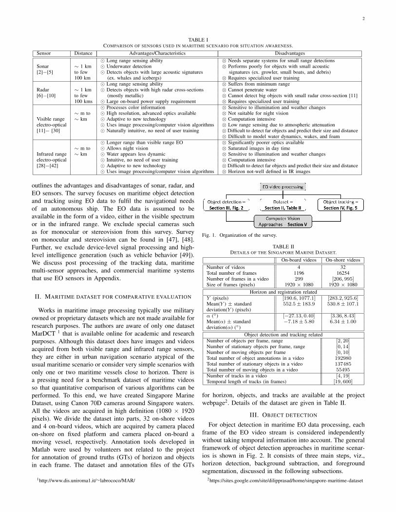
outlines the advantages and disadvantages of sonar, radar, andEO sensors. The survey focuses on maritime object detectionand tracking using EO data to fulfil the navigational needsof an autonomous ship. The EO data is assumed to beavailable in the form of a video, either in the visible spectrumor in the infrared range. We exclude special cameras suchas for monocular or stereovision from this survey. Surveyon monocular and stereovision can be found in [47], [48].Further, we exclude device-level signal processing and high-level intelligence generation (such as vehicle behavior [49]).We discuss post processing of the tracking data, maritimemulti-sensor approaches, and commercial maritime systemsthat use EO sensors in Appendix.

II. MARITIME DATASET FOR COMPARATIVE EVALUATION

Works in maritime image processing typically use militaryowned or proprietary datasets which are not made available forresearch purposes. The authors are aware of only one datasetMarDCT 1 that is available online for academic and researchpurposes. Although this dataset does have images and videosacquired from both visible range and infrared range sensors,they are either in urban navigation scenario atypical of theusual maritime scenario or consider very simple scenarios withonly one or two maritime vessels close to horizon. There isa pressing need for a benchmark dataset of maritime videosso that quantitative comparison of various algorithms can beperformed. To this end, we have created Singapore MarineDataset, using Canon 70D cameras around Singapore waters.All the videos are acquired in high definition (1080 × 1920pixels). We divide the dataset into parts, 32 on-shore videosand 4 on-board videos, which are acquired by camera placedon-shore on fixed platform and camera placed on-board amoving vessel, respectively. Annotation tools developed inMatlab were used by volunteers not related to the projectfor annotation of ground truths (GTs) of horizon and objectsin each frame. The dataset and annotation files of the GTs

1http://www.dis.uniroma1.it/∼labrococo/MAR/

Fig. 1. Organization of the survey.

TABLE IIDETAILS OF THE SINGAPORE MARINE DATASET.

On-board videos On-shore videosNumber of videos 4 32Total number of frames 1196 16254Number of frames in a video 299 [206, 995]Size of frames (pixels) 1920 × 1080 1920 × 1080

Horizon and registration relatedY (pixels) [190.6, 1077.1] [283.2, 925.6]Mean(Y ) ± standard 552.5± 183.9 530.8± 107.1deviation(Y ) (pixels)α (◦) [−27.13, 0.40] [3.36, 8.43]Mean(α) ± standard −7.18± 5.80 6.34± 1.00deviation(α) (◦)

Object detection and tracking relatedNumber of objects per frame, range [2, 20]Number of stationary objects per frame, range [0, 14]Number of moving objects per frame [0, 10]Total number of object annotations in a video 192980Total number of stationary objects in a video 137485Total number of moving objects in a video 55495Number of tracks in a video [4, 19]Temporal length of tracks (in frames) [19, 600]

for horizon, objects, and tracks are available at the projectwebpage2. Details of the dataset are given in Table II.

III. OBJECT DETECTION

For object detection in maritime EO data processing, eachframe of the EO video stream is considered independentlywithout taking temporal information into account. The generalframework of object detection approaches in maritime scenar-ios is shown in Fig. 2. It consists of three main steps, viz.,horizon detection, background subtraction, and foregroundsegmentation, discussed in the following subsections.

2https://sites.google.com/site/dilipprasad/home/singapore-maritime-dataset

3

Fig. 2. General pipeline of maritime EO data processing for object detection.

A. Horizon detection

There are three main approaches for horizon detection −projection based, region based, and hybrid approach. Fig. 3(a)shows three examples of maritime images with horizon. Image1 has two very low contrast targets close to a blurry horizon.Image 2 has horizon characterized by good contrast betweenthe sky and water. Image 3 does not have a well definedhorizon although the presence of the skyline may be a usefulcue for its detection. However, the image suffers from falsehorizontal line created by the wakes of two targets, which islikely to be confused as horizon. Due to a variety of availablecues as well as challenges, we use these images as examples todemonstrate the strengths and weaknesses of different horizondetection methods.

1) Projections from edge map: In these methods, first theedge map of the image is computed using edge detectors [50].It is then projected to another space where prominent linefeatures in the edge map can be identified easily. Typically, theHough and Radon transforms are used for such projections.Given the equation of a line:

x cos(θ) + y sin(θ) = ρ (1)

Each edge pixel with coordinates (x, y) is transformed into acurve in the Hough space (θ, ρ) using the projection [50]:

H(θ, ρ)=

∫∫x,y

(1− δ

(I(x, y)

))δ(x cos θ + y sin θ − ρ) dx dy (2)

where δ represents the Dirac delta function and I(x, y) is theedge map. This is analogous to computing the 2D histogramsof (θ, ρ). Cells in the (θ, ρ) histogram corresponding to fewlargest values of H(θ, ρ) determines the parameters of the line.

The transformation into Radon space is achieved by [50]:

R(θ, ρ) =

∫∫x,y

I(x, y)δ(x cos(θ) + y sin(θ)− ρ) dx dy (3)

Similar to the Hough space, cells in (θ, ρ) with the highestnumber of entries in R(θ, ρ) are the parameters of the line.

While the simplicity of these approaches makes them popu-lar, projective transforms are sensitive to preprocessing such ashistogram equalization and filtering before the extraction of theedge map [50], [51]. Further, they can detect the horizon onlyif it appears as a prominent line feature in the edge map. Thus,as shown in Fig. 3(c,d), both Hough and Radon transformsperform poorly for image 1 but detect the horizon in image2. Although the edge map of image 3 (Fig. 3(b)) does nothave significant features corresponding to the horizon, the cityskyline provides sufficient number of edge pixels parallel andclose to the horizon, enabling a rough detection of horizon.Notably, the wake creates a dark horizontal stripe close tothe targets in image 3 which causes detection of the linecorresponding to the wakes as well.

Fig. 3. Three example images (row a) from [11] and their edge maps (row b)are used for studying the problem of horizon detection. The top 3 candidates,with largest strengths in Hough and Radon spaces are shown in rows (c,d)using colored lines. Average intensity profiles in the vertical direction areshown in (e). The gradients of intensity profiles in (e) are shown in (f).

2) Region based horizon detection: The intensity variationsin the region of the horizon are higher compared to sky orsea regions alone. In Fig. 3(e,f), the mean intensity alongthe vertical axis and its gradient are plotted for images 1−3.The regions of horizon are characterized by significantly largeintensity changes in each of the three images, although theintensity gradient itself is not sufficiently conclusive of thehorizon in image 3. Such localized intensity characteristicsare used for detecting horizon, especially in unmanned aerialvehicles [52], [53], [54]. Quite often, the pixels in an imageare classified as belonging to sky and sea (or ground) [29].

This is a three step procedure. The first step is to use alocal smoothing operator, such as top-hat filter [27], medianfilter [28], mean filter [41], Gaussian filter [55], or standarddeviation filter [41]. The second step is to approximate theselocal statistics with sum of Gaussian functions or polynomialfunctions [17], [32], where each function represents distribu-tion of one region, such as the sea region or the sky region.More complex representations of the regions, such as lineardiscriminant analysis [56], textures [56], covariances [28],[57], and eigenvalues [57], may be used. In the last step, theboundary of two classified regions is identified as horizon. Wenote that region based techniques inherently assume aprioriinformation, such as suitable statistical representations ormachine learning of the trend of intensities at the horizon.

Instead of the second and third steps, Bouma et. al [31] usedhigh intensity gradient to conclude the common boundary ofsea-sky regions and used it as horizon. A more robust versionof this approach employed multi-scale approach [58].III

3) Hybrid methods: The above methods are ineffective forImage 3 in Fig. 3. In such cases, hybrid methods are useful.In the hybrid approach of [60], for each candidate generatedby a projection-based method, the regions above and belowthe candidate line were considered as hypothetical sky andsea regions, and their statistical distributions were computed.The candidate that gives maximum value of the Mahalanobis

4

TABLE IIIHORIZON DETECTION APPROACHES.

Methods Advantages DisadvantagesProjection from edge Radon transform, � Simple ⊗ Sensitive to preprocessingmap [14], [26], [38] Hough transform � Mathematically well-defined ⊗ Work for prominent well-defined linear horizon only

⊗ Horizon may not be the most prominentRegion based Median, correlation, � Work for blurred horizon as well ⊗ Requires statistical apriori knowledge[17], [29], [31], [41] covariance � Suitable for IR images ⊗ Based on statisticsHybrid � More accurate ⊗ More complex[15], [31], [59] �More robust to low-contrast images ⊗ More computation intensive

Fig. 4. Representation of horizon for quantitative comparison of horizondetection approaches is shown in (a). Representative frames from on-boardand on-shore videos are shown in (b,c) respectively.

distance between the distributions of the hypothetical sea andsky regions is chosen as horizon. In [15], local statisticalfeatures were used, but explicit representations of sea andsky regions were not employed. Then, using a set of trainingimages and machine learning techniques, features representinghorizon were learnt directly. Recent algorithms have combinedmulti-scale filtering and projection based approaches for pro-viding state-of-the-art results [61], [62].

4) Comparison of methods for horizon detection: A quali-tative comparison of the methods is provided in Table III. Forquantitative comparison on Singapore Marine dataset, we usethe representation of horizon as shown in Fig. 4(a). Y is thedistance between the center of the horizon and the upper edgeof the frame. α is the angle between the normal to the horizonand the vertical axis of the frame. The ranges and standarddeviations of Y and α are quite large for on-board videos (seeTable II), making them significantly more challenging than on-shore videos. On-board videos are challenging due to presenceof land features very close to horizon, while on-shore videosare also challenging because of the occlusion of horizon byvessels and the presence of wakes in the foreground. Framesfrom both types of videos are shown in Fig. 4(b,c).

We use position error |YGT − Yest| and angular error|αGT − αest| as performance metrics for horizon detection.We provide comparison of Hough transform [28] (referred toas Hough), Radon transform [50] (Radon), mulit-scale medianfilter [31] (MuSMF), Ettinger et. al’s method [53] (ENIW), andFefilatyev et. al’s method [60] (FGSL). Hough and Radon areprojection-based, MuSMF and ENIW are region-based, andFGSL is a hybrid method. We have implemented MuSMF,ENIW, and FGSL since their codes are not available.

The comparison results are given in Table IV. It is notablethat the error in Y is more severe for all the methods ascompared to the error in α. Projection based methods show

TABLE IVQUANTITATIVE COMPARISON OF METHODS FOR HORIZON DETECTION.

THE SMALLEST ERROR IN EACH COLUMN IS INDICATED IN BOLD.Position error Angular error Time/

frame(s)

|YGT − Yest| |αGT − αest|Mean Q25 Q50 Q75 Mean Q25 Q50 Q75

On-board videosHough 219 131 220 295 2.6 0.6 1.7 3.4 0.3Radon 372 213 362 517 40.6 1.5 3.4 87.7 2.7MuSMF 269 156 283 379 1.8 0.5 1.2 2.5 0.9ENIW 120 63 116 166 1.9 0.5 1.2 2.5 hoursFGSL 120 63 117 165 1.8 0.5 1.2 2.5 12.8

On-shore videosHough 208 26 194 354 1.2 0.2 0.7 1.5 0.2Radon 313 28 359 549 32.9 0.2 0.4 88.1 2.0MuSMF 60 25 49 85 1.2 0.2 0.4 1.1 0.9ENIW 121 15 94 163 1.2 0.2 0.4 1.3 hoursFGSL 112 12 91 162 1.2 0.2 0.4 1.1 12.3

poorest performance and statistical methods perform better.MuSMF performs the best for the on-shore videos , FGSLwhich uses both Hough transform and statistical distancemeasure for identifying the horizon performs the best for theon-board videos. MuSMF is parallelizable, with a possibilityof making it about 10 times faster.

B. Static background subtraction

There is a large corpus of works related to backgroundsubtraction that originated from the computer vision commu-nity (see [63] for a review). Maritime background subtractioncan be considered under two scenarios: open seas and closeto port/harbor. In the former, the challenge arises due tothe dynamic nature of the water background in the formof waves, wakes, and debris. In the latter, static structuressuch as buildings or stationary vessels pose a challenge. Thecurrent literature in maritime background subtraction almostexclusively deals with the case of open seas.

The challenge of dynamic background is largely alleviatedif long-wave infrared sensor, such as forward looking infrared(FLIR), is used because it maps the temperature of water,which is relatively uniform despite the dynamicity of water.This suppression of dynamicity occurs to a smaller extent innear-infrared and mid-wave infrared wavelengths [44]. Thus,static background subtraction techniques have better perfor-mance in long-wave infrared regime than in the visible spec-trum. In the following, we describe the various backgroundsubtraction techniques based on background models and theircorresponding learning strategies.

1) Image statistics: Methods in this category use statisticalinformation in a single infrared image. One of the earliermethods is by Bhanu and Holben [15], which modeled animage in terms of gray scale intensity and edge magnitude

5

TABLE VSUMMARY OF STATIC BACKGROUND SUBTRACTION APPROACHES USED IN OBJECT DETECTION.

Approach Model Learning Advantages DisadvantagesSingle imagestatistics [20],[27], [29], [31],[32], [35], [37],[41], [64], [53]

Histogram correlation, polyno-mial functions fitting to stripsparallel to horizon, spatial co-occurrence of intensities, spatialfiltering

No temporal learning, onlyspatial patches/strips are used,initial background typicallylearnt as pixels using spatialstandard deviations

Simple, no learninginvolved, no needof memory

Cannot deal with multi-modal ap-proaches, does not use any form oftemporal information

Gaussian mixturemodel (GMM)[24], [60], [65],[66]

Probability of intensity at a back-ground pixel is a combination ofGaussian functions

Supervised learning usingbackground labelled imagesor videos, adaptive learningcan be used to update GMM

Adapts for multi-modal backgroundand illuminationchanges

Requires supervised learning usinga suitable dataset, adaptive learningmay be complicated

Bayes classifier[21]

Compute the Bayes conditionalprobabilities of the pixel be-ing background (or foreground)given an observed feature vector

Supervised learning through asuitable training dataset

Classification issimple

Learning is complicated and sensi-tive to the training dataset

Feature basedbackgroundclassifier [67]

Compute the feature attributesfor every pixel and determinedistance from pre-learnt classfeatures

Supervised learning of classfeatures using a suitable train-ing dataset with both positiveand negative samples

Robust due to mul-tiple attributes classrepresentation

Computation intensive learning,testing more complex than othermethods above, multi-class mayrepresent wakes, foam, clouds, etc.

with the aim of segmenting the image into foreground andbackground using a relaxation function that gives a lowvalue for background and a high value for the foreground.Similar idea was employed in [68], [69], where, instead of therelaxation function used in [29], confidence maps [68] andchi-squared measure of similarity [69] were used to segmentthe image into background and foreground regions.

Smith and Teal [37] compared the histogram of gray levelintensities in a pixel’s vicinity with a histogram of intensitiesof a reference background. If the histograms were similar,then the pixel was assigned to background. The referencebackground was obtained from the image itself by comput-ing standard deviation over a 3 × 3 window at each pixeland assigning the pixels with less standard deviation as thebackground. The method fails if the reference backgroundis computed incorrectly or if the background has wakes anddebris such that their histograms may not correlate with thereference background histogram.

Van den Broek et. al [32] used horizon to determine thesea and sky regions. It was assumed that intensities in the searegion may vary perpendicular but not parallel to the horizon.Thus, mean and standard deviations of the intensities alongthin strips parallel to the horizon were computed and polyno-mial functions fit upon the mean and standard deviations of thestrips. Similar polynomial fitting was performed for the sky aswell. These polynomial models for sea and sky were then usedto compute a background map and subtract it from the image.This approach removed only low spatial frequency componentfrom the image. Although a more robust approach proposedin [70] was used by [31] for visible range images, naturalhigh spatial frequency components such as due to waves, sun,and clouds were still retained. Gal [71] used a co-occurrencematrix approach to learn sea and sky patterns which weresubtracted from the original image. Fefilatyev et. al [16] usedGaussian low pass filtering in a narrow strip below horizon,followed by a color gradient filter to obtain regions of highcolor variations and finally applied a threshold computed usingOtsu’s method [72] to obtain the background.

Chen at. al [35] considered suppressing repeated spatialpatterns by suppressing peaks in the Fourier transform ofthe image. Spatio-spectral residue and phase map of Fourier

transform of eigenvectors representing 80% of input imagewere used in [20] for background suppression. Multi-scaleapproaches, combined with low-pass filter extracting lowspatial frequencies [73], [74], which are representations ofbackground, have also been found useful. For example, top-hatconvolution filter, which is a low-pass filter, used in a multi-scale approach was shown to be effective in wake suppression[27]. Multi-scale spatio-spectral residue was used in [64].Wang and Zhang [41] used multilevel filter and recursive Otsuapproach [72] to detect and segment very small and either darkor bright targets from images with complex background.

2) Gaussian mixture model (GMM): Although wakes andfoam appear distinct in the visible range images, they arenot entirely suppressed even in infrared images. Thus, thehistograms of both visible and infrared images are invariablymultimodal. Gaussian mixture models (GMM) [75], [76] aresuitable for representing multimodal backgrounds [12], [24],[60], [65], [77]. If a pixel belongs to the background, theprobability P (I) of observing an intensity I at that pixel isgiven as:

P (I) =∑i

wiG(µi, σi) (4)

where G(µi, σi) represents ith Gaussian distribution withmean µi and standard deviation σi, and wi is the weight ofthe ith Gaussian distribution. Fefilatyev et. al [60] representedsky and sea regions as two Gaussian distributions (each beingtrivariate due to the red, green, and blue color channels) fittedwith maximum possible separation between their means. In[24], if the distance of the test pixel’s intensity from the meanof the closest Gaussian distribution was within 2.5 times itsstandard deviation, then the pixel was classified as background.

3) Bayes classifier: Socek et. al [21] used Bayes classifierapproach of [78] for background estimation and suppression.Given the feature vector at a test pixel v(p), if P

(p ∈

B|v(p))> P

(p ∈ F|v(p)

), where B and F indicate

the background and the foreground, then the test pixel wasclassified as the background. The likelihoods P

(v(p)|p ∈ B

)and P

(v(p)|p ∈ F

)were determined through the histogram

of the feature vector, learnt apriori. The supervised learningstrategy enforced that a certain percentage of pixels should beclassified as background using another background estimation

6

TABLE VIQUANTITATIVE COMPARISON OF BACKGROUND SUBTRACTION

APPROACHES FOR ON-SHORE VIDEOS OF SINGAPORE MARINE DATASET.THE BEST VALUES IN EACH COLUMN ARE INDICATED IN BOLD.

Precision (×10−2) Recall (×10−2) Time/frame(ms)Mean Q25 Q50 Q75 Mean Q25 Q50 Q75

Static background subtractionHistComp 0.01 0.00 0.00 0.01 0.06 0.00 0.02 0.05 ∼sStatGMM 0.01 0.00 0.00 0.01 0.08 0.00 0.00 0.03 ∼s

Dynamic background subtractionTempMean 0.07 0.00 0.00 0.00 0.03 0.00 0.00 0.00 43AdaMed 0.25 0.06 0.13 0.26 14.72 6.96 11.00 19.87 61GMM 0.56 0.05 0.29 0.67 9.71 1.91 7.96 13.77 54KDE 0.59 0.08 0.48 0.89 8.93 1.87 9.52 13.31 83OptFlow 11.64 1.65 7.21 14.50 13.35 0.91 6.85 17.99 360IMBS 0.86 0.33 0.62 0.99 7.67 2.23 6.62 11.15 156

CV methods for background subtractionLBP 0.31 0.04 0.27 0.45 3.79 0.67 1.88 4.49 629LBSP 8.00 0.04 3.36 9.29 6.08 0.03 2.73 8.92 589FuzzGMM 0.01 0.00 0.00 0.01 0.06 0.00 0.02 0.05 63FAdaSOM 0.55 0.18 0.32 0.85 11.01 3.07 9.67 13.89 133EigHMM 0.26 0.05 0.14 0.30 14.55 4.68 12.63 18.48 245

method. It was found that the segmented frames containedtoo many noise-related and scattered pixels, which may beseparately classified as outliers and removed, however at theexpense of missing small objects that are few pixels wide.

4) Feature based background classifier: In [67], both fore-ground and background objects were considered as belongingto different known classes, viz., clouds, islands, coastlines,oceanic waves, and ships. It used a total of seven types offeatures, viz., shape compactness, shape convexity, shape rect-angularity or eccentricity, shape moment invariants, wavelet-based features, multiple Gaussian difference features, and localmultiple patterns (discussed more in section V-A7). It alsoconsidered what combinations of features were suitable forimproving the detection accuracy of the different subclasses.

C. Foreground segmentation

In traditional maritime data processing, applying mor-phological operations such as identifying closed boundariesafter background subtraction were considered sufficient forforeground segmentation [21], [23], [79] and the segmentedcontours were used as detected objects. Useful morphologicaloperations for maritime human rescue problem have beenadapted in [79] from [80], [81]. Several interesting edge basedmorphological segmentation techniques for detecting objectshave been discussed in [29]. All are based on consideringobject segmentation as a two-class gray level problem in whichobjects belong to one set of gray levels and the backgroundto the other. A further constraint is that the gradient insidean instance of each class is close to zero and gradients arehigh only along the edges. The underlying assumption inall morphological segmentation approaches is that the objectsare not be occluded and are separate enough such that theirboundaries may not merge.

D. Comparison of static background subtraction techniques

A qualitative comparison is given in Table V. Here, wepresent quantitative comparison of a few static backgroundsubtraction techniques. The foreground is morphologically

Fig. 5. General pipeline of maritime EO data processing for object tracking.

obtained after static background subtraction and enclosed inbounding boxes. They are compared against the boundingboxes of the objects annotated as ground truth. The perfor-mance is evaluated using intersection over union (IOU) ratioof the bounding boxes, defined as

IOU(OGT

i , Odetj

)=

Area(OGT

i ∩Odetj

)Area

(OGT

i ∪Odetj

) (5)

where OGTi and Odet

j are the bounding boxes of ith groundtruth (GT) object and the jth detected object and Area denotesthe number of pixels. If more than one detected objectsoverlap with a GT object, the detected object with maximumoverlap with the GT object is considered associated with theGT and dropped from further associations. The unassociatedobjects or associated objects with IOU less than 0.5 (basedon [82]) are labelled as false positives (FPs). The remainingassociated objects are true positives (TPs). The GT objectsthat are not associated to the any detected objects are labelledfalse negatives (FNs). NTP is the number of TPs in thevideo, analogously for NFP and NFN. Precision and recallare computed as

Precision = NTP/(NTP +NFP) (6)Recall = NTP/(NTP +NFN) (7)

Unfortunately, codes for static background subtraction inmaritime research are not available. We implemented his-togram comparison method (HistComp) of Smith and Teal [37]since sufficient implementation details were available. Further,we implemented a GMM for background subtraction in animage (StatGMM). We used the reference background com-puted in [37] for fitting one GMM each for the red and greencolor channels. Blue channel was not considered since thehistogram of the blue channel’s data is very narrow comparedto the histograms of the other channels for maritime images.Kullback Leibler (KL) divergence [83] of these histogramsfrom the GMMs are determined. In the KL map of each pixel,positive values indicate that the local histograms of the redand green color values are close to the static GMMs. Thisimplementation is intended to serve as the worst performancescenario of GMM for maritime on-shore videos.

The comparison results are presented in Table VI. The his-togram comparison technique of [37] and static GMM performalmost similar, neither providing adequate precision and recall.We note that HistComp was tested on maritime intensity im-ages acquired using low-resolution infrared cameras, and thehigh definition visible range color videos in Singapore-Marinedataset may have caused the poor performance. Similarly, moststatic background subtraction techniques were tested on low-resolution intensity images. Thus, these methods may not besuitable for high-resolution maritime imaging.

7

Fig. 6. The top row shows two consecutive frames and their difference.Second row: result of registration results horizon. Third row: registrationresults using just four fixed points on the shoreline. Fourth row: The fourpoints used for registration in the third row. Saturation and brightness of thedifference images in column (c) have been enhanced for better illustration.SSIM [84] for the image pairs is provided in column (c).

IV. OBJECT TRACKING

In much of the literature related to object tracking inmaritime environment, the problem of object tracking is re-duced to the problem of object detection in every frame. Wedifferentiate between object detection algorithms and objecttracking algorithms in that the latter use (i) temporal informa-tion across frames, e.g. optical flow, and (ii) employ dynamicbackground subtraction algorithms for more robust modelingof the background. A typical pipeline for maritime objecttracking is shown in Fig. 5. Below, we discuss each of themodules in the pipeline.

A. Utility of horizon detection

We discuss the use of horizon detection in object tracking.In object tracking, the main purpose of horizon detection is toallow for registration over consecutive frames and compensatefor the motion of camera or its mounting base (such as due toturbulence of water inducing motion in a boat). Horizon mayalso be used for determining special conditions for detectingobjects close to horizon. For example, [85] used smaller videobricks close to horizon as compared to elsewhere. In somecases, horizon was used as an indicator of the distance betweenthe camera and the vessel being tracked [30] or for motionsegmentation of the vessel [86]. However, sensitivity of thedistance computation to the error in horizon detection wasnoted as severely restrictive in [30], [86].

B. Registration

In maritime scenario, consecutive frames may experiencelarge angular or positional shift. The angular difference maybe due to yaw, roll, and pitch of the vessel. The positional shiftcomes from the fact that the sensor itself is not necessarilymounted at the effective center of motion of the vehicle. If

Fig. 7. Registration using cross-correlation of strip around the horizon. (a)The difference image obtained by registration using horizon only, reproducedfrom Fig. 6. (b) The cross-correlation function of Fefilatyev [59]. (c) Thedifference image after horizontal shift of 48 pixels, identified as the peakin (b). Saturation and brightness of the difference images (a,c) have beenenhanced for better illustration. SSIM [84] for the image pairs is provided.

TABLE VIIQUANTITATIVE EVALUATION OF REGISTRATION APPROACHES ON

ON-BOARD VIDEOS OF SINGAPORE MARINE DATASET.Mean Q25 Q50 Q75 Q90 Time/frame

(ms)Unregistered 0.75 0.66 0.74 0.83 0.98 −Using horizon 0.81 0.75 0.81 0.88 0.94 68Correlation [59] 0.81 0.75 0.81 0.89 0.94 465Feature matching 0.75 0.66 0.73 0.83 1.00 279

the horizon is present, the discrepancy in roll and pitch can becorrected by the change of angle and position of the horizon,respectively. However, the correction of the yaw cannot beachieved. To illustrate this point, consider two consecutiveframes of a video shown in Fig. 6. Horizon based registrationis partially effective (2nd row, 3rd image) but the mismatchalong the horizontal direction indicates that the shift in yawis not corrected. In order to correct for the yaw, we can useadditional features from the scene that can help in registrationas shown in the third row of Fig. 6. However, such featuresare not available in scenes of high seas. Fefilatyev et. al [16],[59] computed normalized cross-correlation in the horizontaldirection along a narrow horizontal strip around the horizon inthe images to be registered. The peaks of the normalized cross-correlation function indicated the amount of shift between thetwo frames. An example is given in Fig. 7.

We present a quantitative comparison of registration tech-niques discussed above on the on-board videos in SingaporeMarine dataset. We used the ground truth of horizon forperforming horizon based registration. For registration usingcorrelation technique of [59], we found that strip of width100 pixels centered at horizon gave the best result. Lastly,we used speeded up robust features (SURF) for registrationusing feature matching. We used all the features that could bematched between a pair of images to perform registration.

We use structural similarity index metric (SSIM) [87] tocompute the similarity between two consecutive frames. It isspecifically suitable for texture matching, and thus a goodmetric for maritime images with dynamic background. Themean SSIM for all the consecutive frame pairs is 0.75, as seenin Table VII. Even the Q25 value of SSIM is 0.66. Registra-tion using horizon and using the cross-correlation technique[59] improves SSIM by 6-7%. However, the Q90 valuesshow a decrease, indicating that some consecutive frames areless similar after registration using horizon only or cross-correlation technique of Fefilatyev et. al [59]. On the otherhand, registration using feature matching hardly improvedSSIM, with improvement appearing in only a few frames as

8

noted from the Q90 value of SSIM. The results indicate thatthe cross-correlation technique [59], although simple, doesnot provide a significant advantage over registration usinghorizon for the current dataset although it was found to beeffective for the videos taken from buoy mounted camera in[59]. We expect that this may be related to either the variety ofstructures seen along the horizon or the angle of the camerawith the sea surface. On the other hand, registration usingSURF features is not effective because of the lack of reliablestationary features in on-board maritime videos.

C. Dynamic background subtraction

As discussed in section III-B, long-wave infrared sensorssuppress dynamicity of water, which is amiss in videosacquired from visible range sensors. If static backgroundmethods are used for such videos, the dynamicity of watercauses incorrect detections. Methods that explicitly modelthe background as being dynamic are more effective in thiscase. Here, we discuss the dynamic background subtractionapproaches used for maritime EO videos processing.

1) Relatively stationary pixels: If a pixel corresponds tosky or water which is relatively stationary in the past fewframes, the temporal distributions of intensities at a pixelover these frames are expected to be unimodal. The meanor median of the distribution is used to determine if thepixel belongs to the background or foreground [18], [37],[88], [89], [90]. A simple threshold approach was used forlearning the background across the frames in [17]. At eachpixel, Lp norm of intensities over a small temporal windowIthresh(x, t) = ‖

(I(x, t′) − I(x, t′)

);∀0 ≤ t − t′ ≤ T‖p was

computed. Here, x and t represent the pixel and the currentframe, T is the size of temporal window, I and I represent theactual and fitted intensities respectively, and ‖ ‖p representsthe Lp norm. The fitted intensity I was obtained by fittinga polynomial over the measured intensities I in the temporalwindow of size T . If

(I(x, t′) − I(x, t′)

)< Ithresh(x, t), the

pixels were assigned to the background.2) Spatio-temporal filtering approaches: Wavelet transfor-

mation was used in [22], [39] for suppressing the background.In [40], wavelet transform and support vector machine on lowfrequency wavelets were used to detect objects, followed bycorrelation over 5 frames, and adaptive segmentation. Lowfrequency wavelets were assumed to contain less informationof clutter and then the uncluttered background would notcorrelate over the frames, thus both clutter and backgroundcould be taken care of.

3) Gaussian mixture models: Gaussian mixture modelshave already been introduced in the context of stationarybackground in section III-B2. In Bloisi and Iocchi [12] fitteda trivariate GMM for RGB values at each pixel over last fewframes. The pixel was labeled as foreground if its RGB valuesdiffered from the GMM by a threshold t that depended uponthe illumination conditions. Gupta et. al [77] also learnt theGaussian model over past few frames only, although usingtime-weighted intensity values. The time weighting allowedfor the GMM to adapt to the changing conditions to asmall extent. A test pixel was classified as background ifthe significance score, proportional to the square of distance

between the intensity of the test pixel and the mean of theGaussian model, was small.

4) Kernel density estimation (KDE): Mittal et. al [19]considered the ocean as dynamic background which wassubtracted to detect people on shore. It used kernel densityestimation (KDE) for background subtraction, in which thebackground model is represented as:

P (It) =1

n

n∑i=1

K(It, κi) (8)

where P (It) is the probability of the intensity at a time tat a given pixel is It, K(I, κ) is the kernel function for theintensity I with kernel parameters specified by κ, and n isthe number of kernels. Typically, single parameter kernels areused. KDE is different from GMM in two respects. First,GMM uses Gaussian kernel whereas KDE allows the kernel tobe asymmetric or have suitable statistical properties. Second,unlike GMM, KDE need not use supervised learning. Typicallyonly a few frames are used for computing the probabilitydistribution and the assumed kernels are fit upon it.

5) Optical flow: Optical flow methods learn the patternsof motion from the videos. The flow vectors computed bycomparing adjacent frames are used to warp each frame withrespect to a reference frame such that stationary componentscan be identified as background. Ablavsky et. al [91] usedoptical flow technique for maritime images, specifically tomodel wakes as background. From a given image frame,pre-learnt motion maps were used to predict next imageframe and correlate it with the actual new frame. The pixelswith high correlation were labelled as background. We notethat optical flow is used as one component in their multi-module interconnected framework for background subtraction.The other components are Bayesian probabilistic backgroundestimation, motion map filter, and coherence analyzer.

6) Multi-step approaches: These approaches combine morethan one technique to achieve better background subtraction.

Independent Multimodal Background Subtraction (IMBS)was proposed by Bloisi et. al [13]. It has three components.The first component is an on-line clustering algorithm. TheRGB values observed at a pixel is represented by histogramsof variable bin size. This allows for modelling of non-Gaussianand irregular intensity patterns. The second component is aregion-level understanding of the background for updating thebackground model. The regions with persistent foreground fora certain number of frames are included as background in theupdated background model. The third component is a noiseremoval module that helps in filtering out false detectionsdue to shadows [92], reflections [93], and boat wakes. Itmodels wakes as outliers of the foreground, forming a secondbackground model specifically for such outliers.

Socek et. al [21] used a four-step process for backgroundextraction: change detection, change classification, foregroundsegmentation, and background model learning and mainte-nance. Change detection was done by subtracting the incomingimage from a reference (pre-learnt) stationary image. Thedetected change image was then analyzed to find if the changescorrelate to the prediction of Bayesian background model [78]or are they likely to be foreground. The regions classified

9

TABLE VIIISUMMARY OF DYNAMIC BACKGROUND SUBTRACTION APPROACHES FOR OBJECT TRACKING.

Approach Model Learning Advantages DisadvantagesRelatively stationarypixels [17], [18], [37],[88]−[90]

Temporal filter extractsstatistical representative ofbackground

Sliding temporal window,change from reference,spatial smoothing

Simple, computation efficient,online learning

Cannot deal with highlydynamic backgrounds, e.g.,wakes

Spatio-temporalfiltering approaches[22], [39], [40]

Background is modelled aslow spatial frequency com-ponent, albeit with temporalvariation

Sliding temporal window andfixed spatial window (blobsor neighborhood) are used forfilter parameters’ update

Simple, online learning, com-putation efficient, robust tosmall dynamics and illumina-tion variation

Cannot deal with highlydynamic backgrounds, e.g.,wakes

GMM [12], [77] Intensities at a pixel as mix-ture of Gaussian distribu-tions

Fitting GMMs on histogramsof intensities over past fewframes

Online, less memory intensive,simple, adaptive

Cannot accommodate complexintensity distributions and sud-den illumination changes

Kernel densityestimation[19]

Background modelled assum of kernels of adaptivespreads

Learnt through fitting overlast few frames

Asymmetric kernels may beused, online learning, fast andadaptive, can deal with smallillumination variations, wakes,and foam better than GMM

Kernels should be good rep-resentative or else several ker-nels may be needed, adaptivenature makes it sensitive tovariations

Optical flow [91] Segment initial background,compare with backgroundpredicted by motion map

Learnt by spatial gradients’patterns over time as veloc-ities

Suitable for wakes, big waves,and clouds

Not suitable for random wavemotion, computation intensive

Multi-stepapproaches [13],[21]

Combination of more than one technique More robust and versatile, of-ten made adaptive and capableof dealing with wakes

Complicated, computation in-tensive, slow due to frequentfeedback —feed-forward steps

as foreground were then used with color-based segmentationapproach to further strengthen the foreground estimation andthus contribute to more robust background detection. Thebackground thus determined was used to update the referencestationary image and the Bayesian background model.

7) Comparison of techniques for dynamic background sub-traction: A qualitative comparison of the dynamic backgroundsegmentation methods is given in Table VIII. In this sec-tion, we compare the performance of dynamic backgroundsubtraction techniques for the on-shore videos in SingaporeMarine dataset. We have used the on-shore videos only toensure that the dynamics correspond to the scene only andnot to the sensor. The metrics and methodology of comparisonare the same as discussed in section III-D. Since the sourcecodes or executables of the methods for maritime dynamicbackground subtraction are not available, with the exceptionof IMBS [13], we have used temporal mean (TempMean)background model implementation of [94] as an example oftechniques that use the concept of relatively stationary pixels,adaptive median filtering (AdaMed) [95] as an example ofspatio-temporal filtering approaches, Gaussian mixture model(GMM) of [96], kernel density estimation (KDE) of [97],Lucas-Kanade approach [98] for optical flow (OptFlow) basedbackground subtraction, and IMBS as an example of multistepapproaches for background subtraction. We used the computervision toolbox of Matlab for optical flow segmentation usingLucas-Kanade [98] approach. The video was scaled down to0.5 times its actual size in pixels before computing the opticalflow. Bounding boxes with dimensions less than 10 pixels inthe scaled down frames were filtered away to suppress themotion due to water. The remaining bounding boxes were usedafter scaling up to the original dimensions. For IMBS [13], wehave used the source code of the authors. For the rest, we haveused the codes in the background subtraction library [94].

The comparison results are shown in Table VI. With theexception of temporal mean approach, the other dynamicbackground subtraction approaches invariably perform betterthan the static background subtraction approaches. Further, the

noticeably better precision of optical flow based approach isattributed to the down-scaling of the frames which suppresseddetection of extremely small spurious characteristic of motionof water and the filtering away of small foreground segmenta-tions. In terms of recall, the adaptive median approach of [95]performs the best, despite being simple. Nevertheless, none ofthe methods provide practically useful precision and recall.

D. Tracking

In a typical object tracking pipeline, objects are extractedby background subtraction and segmented before they aretracked. However, in some cases, tracking is done even withoutsegmenting the background, as discussed in section IV-D6.

1) Basic tracking techniques: Hu et. al [18] formulated theproblems of tracking as computation of an adaptive boundingbox, where the bounding box in current frame is an adaptationof the bounding box in the previous frame within specifiedranges of adaptivity to compensate for the background mis-match between the current and previous frames. Temporal highpass filter (analogous to fast moving objects) of segmentedshapes was used in [23]. Robert-Inacio et. al [44] tested thelocations of the objects in consecutive frames for expectedspeed range. Objects were tracked as long as such speed of theobject persists. Westall et. al [79] used dynamic programmingfor tracking of the objects in the videos.

2) Feature based tracking: Methods in which prominentfeatures of the objects are used for tracking are more suitablefor dealing with occlusion. Bloisi et. al [14] used Haar featuresfor detecting and tracking objects. It is notable that [14]used visible range color images as input and their featuresdetection strategy for color images may not be directly usefulfor IR images. Other key point detectors, such as Harris cornerdetector, were found to be more effective [99].

3) Shape tracking with level-sets: Casting segmentedshapes (shape contours) as level-sets [65], [11] and thenevolving the level-sets over frames has also been found usefulfor tracking. Notably, level-set techniques generally requirethe number of foreground objects and their initial contours to

10

TABLE IXSUMMARY OF TRACKING APPROACHES USED IN MARITIME OBJECT TRACKING.

Approach Model Learning Advantages DisadvantagesBasic trackingtechniques [18],[23], [44], [79]

Adaptive bounding box, Temporalhigh pass filter

Online using a small tem-poral window and memoryof previous tracking

Simple, computation effi-cient, adaptive boundingbox can deal with wakes

Naive, non-predictive

Feature basedtracking [14],[99]

Track features of segmented objects Match features acrossframes

More robust than shapetracking, may allowsome deformation (aspectchange)

Features may not be consis-tently present, selection of ap-propriate features is important,computation intensive

Shape trackingwith level-sets[11], [65]

Segmented shape contours are castinto level sets

Level sets are evolvedthrough the frame

Apriori knowledge not re-quired, but beneficial

Cannot deal with occlusion,sensitive to shape segmenta-tion, computation intensive

Bayesianpredictivenetwork [79]

Features of objects case as state vec-tors of network representing motionmodel

Learning techniques suchas expectation maximiza-tion are used to progres-sively update the network

Predictive nature, learnsmotion adaptively

Requires features as state vari-ables, very computation inten-sive, cannot deal with complexmotion patterns

Kalman filters[12], [16], [26],[60], [100]

Motion model is represented as statevector at a time t, current foregroundsegmentation’s feature is case as inputvector (to update the state vector) andGaussian random motion perturbationis cast as noise (to be filtered)

State vector is updatedfor least square error be-tween the actual measure-ment (input) and the pre-dicted measurement (usingprevious state vector)

Almost real time, can fil-ter away random perturba-tions, can adapt to multi-ple objects, can deal withcomplex motion variationsoccurring slowly

Does not work for complexrandom small motions, needsspecial framework for multipleobject tracking

Optical flow[12], [19]

Computes motion maps or flow vec-tors to determine consistent motionpatterns

Cluster using modified k-means clustering on flowmaps or compute flowequation at each pixel

Wakes and waves are au-tomatically suppressed dueto inconsistent motion pat-terns

Cannot deal with boat maneu-vers and is computation inten-sive

be specified [65], [11]. On one hand, knowing the numberof objects require pre-segmentation of the objects, even ifcrude estimates are used. On the other hand, specifying initialcontours imply that occluded objects may be difficult to dealwith in such techniques. The level-set based approaches canbenefit from some shape prior [65] which may be knownthrough the general geometry knowledge of the expectedobjects (sea vessels of various kinds for maritime problem).

4) Bayesian predictive network: In the Bayesian ap-proaches for tracking, the objects or features in a frame tobe tracked are considered as a state vector of the Bayesiannetwork and the training of a predictive model for transitionbetween states is done to obtain a predictive model [79].Often, once a Bayesian network is trained, it can be usedto predict the state of the next frame given the state(s) inthe previous frame(s). Thus Bayesian networks and hiddenMarkov models are suitable for tracking of objects that havea relatively smooth or predictable motion. They are suitablefor dealing with multiple objects as well as occlusion as theobjects’ locations and features in a frame can be assigned astate variable each while the occlusion can be dealt with dueto the predictive nature of the networks. However, it is difficultto make them adaptive and thus agile to learn complex motioncharacteristics such as some objects becoming stationary forsome time.

5) Kalman filters: Tracking large objects such as ships inport environment was performed using a mixture Kalman filterapproach in [100]. Kalman filters were used in [101], [102] forlearning the motion of the foreground objects. In the originalform, Kalman filters cannot deal with multiple hypotheses, ormultiple object motion tracking simultaneously [103]. Thus, amulti-hypotheses Kalman filter for tracking was proposed in[104] and its optimal implementation was presented in [105].It was found useful in maritime problems [12], [16], [26], [60].

It was reported in [12] that the multi-hypotheses Kalmanfilter approach provides a good balance between computation

load and tracking robustness. We note that Bloisi and Iocchi[12] tested this on high resolution video stream and its validityon lower quality videos is not assured. Wei et. al [26] usedmanually pre-assigned initial tracks and simple Kalman filtersto track the objects instead of multi-hypotheses Kalman filters.

6) Motion segmentation using optical flow approach:Direct foreground tracking without pre-segmenting the fore-ground can be done by ’motion segmentation’. The spatialinformation is incorporated implicitly as the features or pixelswith same motion characteristics are likely to belong to thesame foreground object. Although several motion segmenta-tion approaches are used in the computer vision, as discussedlater in section V-B, methods for maritime EO problem haveused optical flow based motion segmentation only [12], [19].The underlying assumptions in optical flow based techniquesare that the objects are rigid and the motion is smooth.

Bloisi et. al [12] first computed connected segments in theforeground, which are not necessarily the foreground objects.Then, they computed sparse motion maps for each blob. Thewakes and shadows do not have a consistent motion map andthus are suppressed in the optical flow approach. In order todeal with multiple foreground objects in one blob, a modifiedk-means clustering approach was applied on the optical flowmap. First the motion map was over-clustered into manysmall clusters using k-means clustering. Then, the clusterswere iteratively merged till further merging reduced the clusterseparation instead of increasing the cluster separation. Notably,optical flow method fails in boat maneuvers because the opticalflow may detect different directions for the different partsof the boat. Further, two boats having very similar motioncharacteristics and present in one blob cannot be separated byoptical flow as well as k-means clustering.

Mittal et. al [19] computed the optical flow velocity vector fby solving the flow constraint equation ∇g ·f+gt = 0, whereg is the measured value of a color channel, ∇g is the gradientof g, and gt is the temporal derivative of g. This equation was

11

solved at each pixel such that the error in the estimated flowvector f is minimised while satisfying the constraint that thevelocity f is locally constant.

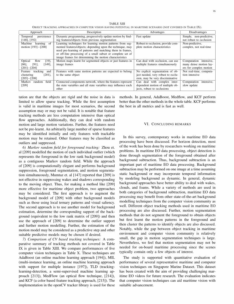
7) Comparison of techniques for tracking: A qualitativecomparison is given in Table IX. Here, we present a per-formance comparison of techniques of tracking on on-shorevideos of Singapore Marine dataset. We have used only on-shore videos so that the performance of tracking is not biaseddue to camera’s motion. Performance metrics for tracking[106], namely precision, recall, multiple object tracking ac-curacy (MOTA), multiple object tracking precision (MOTP),and false alarm rate (FAR) are used, which we describe below.

An ith ground truth (GT) track is represented by its GTbounding box OGT

i,t in frame t. Analogously, Odetj,t denotes

the bounding box of the jth track at time t detected by atracking technique (simply referred to as a tracker). Then,for ith ground truth track and jth detected track, IOU(i, j, t)denotes the value of IOU computed using eq. (5) for the pair(OGT

i,t ,Odetj,t ) at frame t. Matched pairs of ground truth tracks

and detected tracks are determined using Hungarian method[107] with 1− r(i, j, t) as input, where r(i, j, t) is defined as

r(i, j, t) =

{IOU(i, j, t) if IOU(i, j, t) > 0.5

0 otherwise(9)

Hereafter, (i, j) denotes a matched pair of ith ground truthtrack and its corresponding jth detected track. In a frame t, allunmatched ground truth tracks contribute to one false negative(FN) each and all unmatched detected tracks contribute to onefalse positive (FP) each. For the matched tracks, if IOU(i, j, t)is more than 0.5 (based on [106]), the detection is said to betrue positive (TP) for that frame. Otherwise it contributes toa mismatch (MM). Thus, NTP,t, NMM,t , NFP,t, and NFN,t

are the numbers of TPs, mismatches, FPs, and FNs in a framet. Further, total number of matched pairs of ground truth anddetected tracks in a frame t irrespective of the values of IOUis given as NM,t = NTP,t + NMM,t and the total number offrames in the video is denoted as T . Precision, recall, FAR,MOTA, and MOTP are then defined as

Precision =

∑tNM,t∑

t (NM,t +NFP,t)(10)

Recall =

∑tNM,t∑

t (NM,t +NFN,t)(11)

FAR =∑t

NFP,t/T (12)

MOTA = 1−∑

t (NFP,t +NFN,t +NMM,t)∑t (NM,t +NFN,t)

(13)

MOTP =

∑(i,j),t

r ((i, j), t)∑tNM,t

(14)

Precision and recall have their usual range of [0,1] with bestvalues being 1. The unit of FAR is number of false positivesper frame and its value may be any non-negative real number,with 0 being the best value. MOTA may take negative valuesbut has a maximum and best value of 1. MOTP lies in therange [0,1], the best value being 1.

TABLE XQUANTITATIVE EVALUATION OF DIFFERENT TRACKING TECHNIQUES FORON-SHORE VIDEOS OF SINGAPORE MARINE DATASET. THE BEST VALUES

FOR EACH METRIC ARE HIGHLIGHTED USING BOLD FONT.Techniques related to maritime

Metric MST KLT DAOT MOT LKDoG

Precision

Mean 0.57 0.73 0.65 0.01 0.00Q25 0.38 0.60 0.53 0.00 0.00Q50 0.52 0.70 0.65 0.01 0.00Q75 0.83 0.86 0.77 0.01 0.00

Recall

Mean 0.53 0.77 0.68 0.04 0.02Q25 0.31 0.68 0.57 0.0.00 0.00Q50 0.50 0.76 0.68 0.03 0.01Q75 0.77 0.88 0.82 0.06 0.02

MOTA

Mean 0.15 0.47 0.29 -6.45 -11.79Q25 -0.20 0.20 0.07 -8.36 -10.02Q50 0.05 0.45 0.32 -5.43 -8.00Q75 0.59 0.72 0.59 -4.07 -5.67

MOTP

Mean 0.74 0.80 0.68 0.61 0.45Q25 0.71 0.76 0.66 0.59 0.51Q50 0.74 0.81 0.68 0.60 0.55Q75 0.77 0.82 0.69 0.62 0.59

FAR

Mean 3.46 2.70 3.56 46.85 81.10Q25 0.97 0.91 1.16 42.21 46.45Q50 2.66 2.43 2.83 48.73 58.36Q75 5.79 4.40 5.20 52.43 81.17

Time/frame (s) 1.66 0.51 0.73 0.26 1.14Other computer vision techniques

Metric AdaBoost MIL TLD MedFlow KCF

Precision

Mean 0.82 0.62 0.26 0.76 0.86Q25 0.68 0.48 0.16 0.69 0.77Q50 0.86 0.71 0.26 0.75 0.90Q75 0.91 0.78 0.35 0.86 0.96

Recall

Mean 0.83 0.63 0.27 0.77 0.87Q25 0.75 0.48 0.16 0.72 0.79Q50 0.85 0.70 0.27 0.79 0.90Q75 0.92 0.79 0.36 0.84 0.95

MOTA

Mean 0.64 0.23 -0.50 0.52 0.72Q25 0.46 -0.03 -0.71 0.39 0.55Q50 0.66 0.42 -0.49 0.52 0.80Q75 0.83 0.54 -0.30 0.68 0.89

MOTP

Mean 0.79 0.75 0.63 0.79 0.80Q25 0.77 0.69 0.60 0.76 0.78Q50 0.80 0.75 0.63 0.79 0.80Q75 0.82 0.80 0.65 0.83 0.83

FAR

Mean 1.73 3.52 6.56 2.24 1.37Q25 0.70 1.51 4.07 1.17 0.19Q50 1.13 2.45 6.21 1.57 0.91Q75 2.37 4.99 8.53 3.35 2.09

Time/frame (s) 12.03 3.31 42.73 0.42 0.47

We consider one technique per row of Table IX, with theexception of level-set based tracking, for which we could notfind an implementation. We use mean shift tracking3 (MST)[111] as an example of basic tracking techniques, Kanade-Lucas-Tomasi (KLT) feature tracker4 [98], [112] for fea-ture based tracking, distractor-aware online tracking (DAOT5,[113]) for tracking using Bayesian predictive network, motion-based multiple object tracking4 (MOT) using Kalman filter[114] for Kalman filter based tracking, and optical flow basedon Lukas-Kanade difference of Gaussian method4 (LKDoG,[115]). No background subtraction technique has been appliedin order to compare the performance of tracking only. MST,KLT, and DAOT are single object trackers and require initialguess (we used the first bounding box of each GT track). MOT

3https://www.mathworks.com/matlabcentral/fileexchange/35520-mean-shift-video-tracking

4Matlab provided function5Matlab code provided by the authors of [113])

12

TABLE XISUMMARY OF LITERATURE ON OBJECT DETECTION AND TRACKING IN

MARITIME SCENARIO.

Articles YearEO Scene Object Object

sensor detection tracking

Infr

ared

Vis

ible

On

shor

e

Ope

nse

a

Hor

izon

dete

ctio

n

Stat

icba

ckgr

ound

Fore

grou

ndse

gmen

tatio

n

Hor

izon

dete

ctio

n

Reg

istr

atio

n

Dyn

amic

back

grou

nd

Fore

grou

ndtr

acki

ng

Bhanu [29] 1990 • • •Sumimoto [23] 1994 • •Strickland [22] 1997 • •Smith [37] 1999 • •Broek [32] 2000 • • • •Voles [85] 2000 • • •Caspi [108] 2002 • • • • •Ablavsky [91] 2003 • •Mittal [19] 2004 • • •Socek [21] 2005 • • • •Fefilatyev [15] 2006 • • • •Wang [40] 2006 • • •Robert- 2007 • • • • •Inacio [44]Schwering [36] 2007 • • •Bouma [31] 2008 • • • • • •Broek [30] 2008 • • •Zheng [109] 2008 • •Bloisi [12] 2009 • • •Gupta [77] 2009 • • •Haarst [17] 2009 • •Wei [26] 2009 • • • •Fefilatyev [16] 2010 • • • • • • •Zhu [67] 2010 • •Bloisi [14] 2011 • • •Hu [18] 2011 • • • •Szpak [11] 2011 • • •Wang [41] 2011 • • •Broek [99] 2012 • • • •Ren [20] 2012 • •Zhang [66] 2012 • • •Frost [65] 2013 • •Gershikov [28] 2013 • • •Tang [38] 2013 • • •Bloisi [13] 2014 • •Broek [33] 2014 • • • •Broek [34] 2014 • • • •Chen [35] 2014 • • •Tu [39] 2014 • •Wang [24] 2014 • • • •Zhou [27] 2014 • •Babaee [110] 2015 • •Wang [25] 2015 • •

and LKDoG do not require initial guess and track multipleobject simultaneously. The results are presented in Table X.MST, KLT, and DAOT clearly benefit from the initial guessbecause the number of tracks remains close to the actualnumber of ground truth tracks. On the other hand, MOTand LKDoG suffer due to large number of false positives asa consequence of water dynamics. Among MST, KLT, andDAOT, MST performed the best in terms of all the metrics.

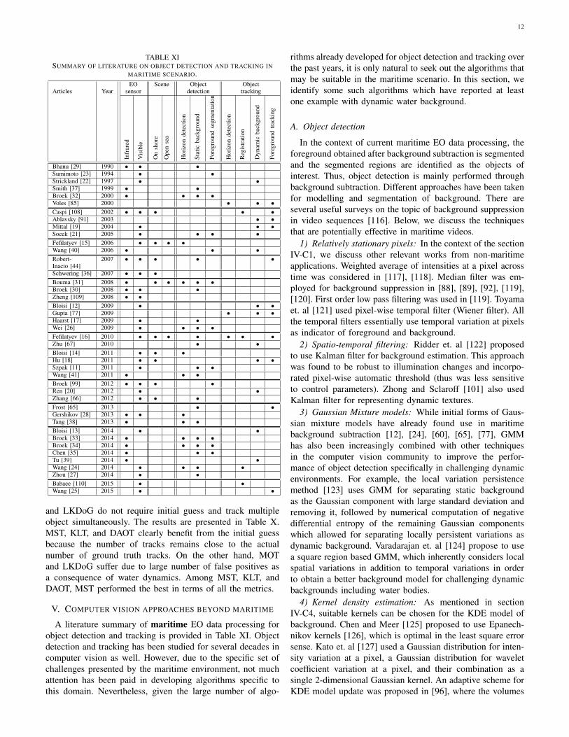
V. COMPUTER VISION APPROACHES BEYOND MARITIME

A literature summary of maritime EO data processing forobject detection and tracking is provided in Table XI. Objectdetection and tracking has been studied for several decades incomputer vision as well. However, due to the specific set ofchallenges presented by the maritime environment, not muchattention has been paid in developing algorithms specific tothis domain. Nevertheless, given the large number of algo-

rithms already developed for object detection and tracking overthe past years, it is only natural to seek out the algorithms thatmay be suitable in the maritime scenario. In this section, weidentify some such algorithms which have reported at leastone example with dynamic water background.

A. Object detection

In the context of current maritime EO data processing, theforeground obtained after background subtraction is segmentedand the segmented regions are identified as the objects ofinterest. Thus, object detection is mainly performed throughbackground subtraction. Different approaches have been takenfor modelling and segmentation of background. There areseveral useful surveys on the topic of background suppressionin video sequences [116]. Below, we discuss the techniquesthat are potentially effective in maritime videos.

1) Relatively stationary pixels: In the context of the sectionIV-C1, we discuss other relevant works from non-maritimeapplications. Weighted average of intensities at a pixel acrosstime was considered in [117], [118]. Median filter was em-ployed for background suppression in [88], [89], [92], [119],[120]. First order low pass filtering was used in [119]. Toyamaet. al [121] used pixel-wise temporal filter (Wiener filter). Allthe temporal filters essentially use temporal variation at pixelsas indicator of foreground and background.

2) Spatio-temporal filtering: Ridder et. al [122] proposedto use Kalman filter for background estimation. This approachwas found to be robust to illumination changes and incorpo-rated pixel-wise automatic threshold (thus was less sensitiveto control parameters). Zhong and Sclaroff [101] also usedKalman filter for representing dynamic textures.

3) Gaussian Mixture models: While initial forms of Gaus-sian mixture models have already found use in maritimebackground subtraction [12], [24], [60], [65], [77], GMMhas also been increasingly combined with other techniquesin the computer vision community to improve the perfor-mance of object detection specifically in challenging dynamicenvironments. For example, the local variation persistencemethod [123] uses GMM for separating static backgroundas the Gaussian component with large standard deviation andremoving it, followed by numerical computation of negativedifferential entropy of the remaining Gaussian componentswhich allowed for separating locally persistent variations asdynamic background. Varadarajan et. al [124] propose to usea square region based GMM, which inherently considers localspatial variations in addition to temporal variations in orderto obtain a better background model for challenging dynamicbackgrounds including water bodies.

4) Kernel density estimation: As mentioned in sectionIV-C4, suitable kernels can be chosen for the KDE model ofbackground. Chen and Meer [125] proposed to use Epanech-nikov kernels [126], which is optimal in the least square errorsense. Kato et. al [127] used a Gaussian distribution for inten-sity variation at a pixel, a Gaussian distribution for waveletcoefficient variation at a pixel, and their combination as asingle 2-dimensional Gaussian kernel. An adaptive scheme forKDE model update was proposed in [96], where the volumes

13

(spreads) of the kernels were made adaptive by changing thenumber of frames considered for the dynamic update.

5) Optical flow: Ross [128] presented an interesting con-cept of texture-and-motion duality in optical flow in orderto extract background. It used the single image segmentationapproach of [129] to get an initial estimate of the background.Optical flow of the segmented regions was computed usingan energy minimization approach [130]. Li and Xu [131]perform optical flow computation directions at the edges ofsuper-pixelated regions to enhance the computation speedwhile allowing the identification of super-pixelated regionsbelonging to the dynamic background owing to the non-uniform flow vectors at their edges.

6) Range model: A simple and popular approach for dy-namic background extraction was considered in [132] whichused a range of intensity values for a given pixel, quantified byminimum and maximum intensity values at a background pixeland maximum intensity difference between two consecutiveframes, denoted as m(x), n(x), d(x), respectively. For findingthe parameters of this model, the pixel’s intensity values ina reasonably long time sequence I(x, t) were used. First, theinstances t′ at which pixel can be considered as stationarywere found as

|I(x, t′)− λ(x)| < 2σ(x) (15)

where λ(x) and σ(x) are the mean and standard devia-tion of I(x, t),∀t. Then, m(x) = min(I(x, t′), n(x) =max(I(x, t′), d(x) = max(|I(x, t′) − I(x, t′ − 1)|) werecomputed. The model parameters may be updated as oftenas needed. Haritaoglu [132] also suggested a technique foridentifying that a moving object in earlier frames has becomea stationary background in later frames.

Kim et. al [133] used a codebook of possible range valuesfor addressing multi-class background. The code of a classwas given by the range parameters discussed above. Thiswas further augmented by average color data, frequency ofoccurrence of the code, and last access of the code.

7) Dynamic textures: Local binary pattern [134] (LBP),either at a single pixel, or a small region around the givenpixel [135], finds a binary number representing the booleanintensity changes in the neighborhood of the chosen pixel.It may be made shift and rotation invariant, as discussed in[134]. The LBP feature vector of a block of pixels in a frameis the histogram of the binary numbers obtained at all thepixels in the block [171]. Over time, one LBP feature vectoris obtained for each frame and the net background featurevector is a weighted combination of feature vectors of the lastK (often heuristically chosen) number of frames. A distancemeasure for decision making and a model update schemeis discussed in [135]. This approach was found useful inapplications involving underwater videos [136], [137]. Localbinary similarity patterns (LBSP) [172] are a variation ofLBP and include spatio-temporal binary similarity metric. Amodification of LBP to deal with flat regions in an image isthe local ternary patterns (LTP), presented and discussed in[135], [138], [139], [140]. Furthermore, [141], [142] proposeda mixture of dynamic textures, analogous to GMM, in orderto allow for modeling of multiple dynamic textures. Mixture

of dynamic textures showed good ability to deal with ocean’sdynamic texture with synthetic translucent objects and flames.

8) Hidden Markov model of dynamic background: HiddenMarkov models (HMM) have two specific advantages ascompared to other modelling approaches [127]. The first isits ability to incorporate temporal continuity. A pixel may beclassified as belonging to background, foreground, or shadowin a particular frame. Nevertheless, it is likely that the pixelwill have the same classification for at least a few continuousframes. This is so either because the object at the pixel isstationary or because the moving object occupies the pixelsfor some number of frames till the object crosses the pixelcompletely. HMM is inherently able to cover both thesepossibilities. Second, HMM does not require a specificallychosen training data. A scenario specific ordinary imagesequence is sufficient for it to learn the hidden states that allowdemarkation between background, foreground, and shadows.Further, it was noted in [116] that HMM approach is veryeffective in dealing with sudden illumination changes andproviding a corrective temporary estimate of the backgroundin such scenario.

Thus, despite being computationally expensive and difficultfor dynamic modification of topology [116], [128], HMM hasattracted a lot of attention for background suppression [21],[143], [144], [145], [146], [162]. One of the most recent worksin this context is [147], which showed some examples of boatsin sea as well. It has many interesting and useful features,which include using dynamic textures [173] for simultaneousforeground-background modelling, augmenting the dynamictextures by introducing spatially smooth segmentation throughHMM [141] and a specially designed expectation maximiza-tion approach with variational constraint.

We briefly discuss the update methods used for learning andupdating the HMMs. Sheikh and Shah [148] used Markovrandom field with maximum-a-posteriori estimation to ob-tain spatial context in a simultaneous foreground-backgroundmodeling approach. Expectation maximization approaches fortraining HMM have been discussed in [143], [174], [175].Stenger et. al [146] designed a dynamic update scheme forHMM which allows for adaptive topology modification of theHMM. Ostendorf and Singer [176] suggested that dynamicadaptation of HMM can be made fast by a state splitting ap-proach. Brand and Kettnaker [177] suggested that an arbitrarilylarge number of states may be initially chosen and then entropybased training of HMM may be used to identify the lessprobable states and iteratively remove them. Wang et. al [178]used an offline Baum Welch algorithm [179] to learn HMM butemployed an online algorithm for background detection andupdating the HMM. Rittscher at. al [144] proposed a schemefor making HMM computationally less expensive and almostreal-time. Brand and Kettnaker [177] and Ostendorf and Singer[176] discussed the optimal choice of number of states ofHMM. Further, some amount of speed up of the HMM updatemay be achieved using subspace based approaches [101],[145].

9) Saliency based approaches for segmenting the back-ground: Wixson [149] used a saliency measure defined onthe cumulative optical flow directions of the moving objects

14

TABLE XIIBACKGROUND SUBTRACTION APPROACHES IN COMPUTER VISION HAVING POTENTIAL IN MARITIME SCENARIO (NOT COVERED IN TABLES V AND VIII).

Approach Description Advantages DisadvantagesRange model [132], [133] Multiple class model, each with a range

of intensitiesSimple, pre-learnt ranges, may be madeadaptive

Not discriminative

Local binary and ternarypatterns [134]−[142]

Background model representing dy-namic textures

Multiple patterns may be learnt for differ-ent dynamic textures such as water, wake,and waves, quite robust, can be learnt andadapted online

Computation intensive

Hidden Markov model[21],[127]−[148]

Local intensities (or other features) asstate vectors in HMM

Uses temporal continuity of classification,does not require any pre-learning

Complex, computation intensive

Saliency based approaches[149]−[152]

Approaches for classifying pixels asbackground based on the used back-ground model

More sophisticated than a simple thresholdor range; can incorporate certain proper-ties for classification, such as discriminativeproperty and surprise

Complex, may be computation in-tensive

Fuzzy classifiers[153]−[156]

Fuzzy techniques for classification ofpixel as background

Needs appropriate fuzzy classifier functionsto be pre-learnt

Complex, needs supervised learn-ing of classifier functions

Subspace basedapproaches [25], [66],[69], [101], [138], [145],[151], [157]−[170]

Learning the background model, com-pactly representing and fast updating ofthe model, finding the overlap of pixelfeatures with the model

Fast, compact, amenable to fast linear pro-gramming

Assume linear separability of data,degrade with large dynamics inbackground

(foreground). It incorporates net flow directions by computingmaximum flow directions and finding observations consistentwith the maximum flow direction. Such saliency measurebased on maximum flow direction may be suitable for singleobject tracking but may need significant modification forincorporating multiple object tracking. On the other hand, Ittiet. al [150] used a surprise based saliency map to segregatethe non-surprising elements as the background (low saliency).It determined a surprising element as an element which hasa large contrast compared to the surrounding pixels. Thecontrast should be consistently present at various length scales.This contrast is referred to as the center-surround difference.Although it can deal with the wavy nature of water to someextent, it is not effective in suppressing the wakes since theyintroduce a high contrast with respect to their surroundings.

Gao et. al [151] modified the saliency approach of [150]by retaining the center-surround and multi-scaling. It useddiscrimination (referred to as discriminant in [151]) betweenintermediate features in the center-surround instead of usingthe direct contrast feature [150] directly. It was tested onvideos of floating bottle and surfer and showed better back-ground identification than [150]. We note that [151] used localternary patterns as the features of the background model.

Mahadevan and Vasconcelos [152] combined the discrim-inant saliency approach of [151] and mixture of dynamictextures [142] for determining spatially normal (high prob-ability distributions) and temporally normal (high probabilityevents) features of the videos with the moving crowd in urbanscenarios. Furthering this concept, Wang et. al [178] proposeda saliency metric called spatiotemporal condition information(SCI). This metric computes the conditional information value(logarithm of conditional probability) of a pixel given thebackground and the spatiotemporal neighborhood of the pixel.Larger value of the conditional information indicates higherlikelihood of the pixel being foreground.

Fang et. al [180] computed two saliency maps, one charac-terizing spatial saliency through proximity and continuity ofa visually salient object region and the other characterizingtemporal saliency which accounts for dynamic backgroundvariation and persistence of local contrast. These maps are

merged by using an adaptive entropy-based uncertainty weigh-ing approach to form the final spatiotemporal saliency map.

Recently, Liu et. al [181] used motion saliency map of [182]to determine the control parameter of the robust principlecomponent analysis [158], which was then used for back-ground subtraction and foreground extraction. In this definitionof motion saliency, the sum of the background motion mapM such as due to water dynamics in maritime scenarioand the stable background map B is said to be a low rankrepresentation of the video V . The background motion mapand the stable background are solved by minimizing the sumof nuclear norm of B and L1 norm of M .

10) Fuzzy classification of background pixels: Fuzzy logicwas used to compute an adaptive threshold for classifying thebackground pixels in complex background in IR images [153],[154], [155]. Although most of the experiments are in urbanand semi-urban land scenarios, the techniques may inspirefurther interesting work in maritime IR images. A combinationof fuzzy neural network and self organizing map [183] wasused in [184]. It is shown to be robust to illumination changesand shadows, a property beneficial for maritime videos. In[185], the usual GMM background model was modified to befuzzy mixture of Gaussian functions.

11) Subspace based approaches in background modellingand subtraction: Spatio-temporal block of images, the collec-tion of all the features of background model and the featureattributes of all the pixels may be represented as matrices.Then matrix decompositions can be used for manipulatingthe data, learning the model, compactly representing and fastupdating the model, as well as finding the overlap of pixelfeatures with the model in a powerful manner.

Thus, subspaces based approaches have been found useful[186] for compact representation of features at pixels beforelearning is performed. These include eigenbackground ap-proach [66], [187], [188], [162], principal component analysis(PCA) [157], [161], [162], robust PCA [158], [189], indepen-dent component analysis [159], [190], and discriminant centersurround [151], [160]. Subspace based learning was usedfor night-time videos as well in [191]. It is anticipated thatthese approaches may be improved by suitable combination of

15

eigenvectors of the data and designing a robust update schemefor the background.

Autoregressive updates of background models is done byidentifying the subspace of consistently recurring backgrounds[101], [138], [121], [163]. Methods in [69], [164], [165]that use correlation or covariance approaches may also beconsidered as subset of approaches that employ backgroundsubspace analyses. Some methods also use sparsity priorsand implement background detection problem as sparse im-age reconstruction problem [145], [166], [167], [168], [169].Alternatively, compressive sampling based approaches can beused to reduce dimensionality of the data before using otherbackground detection techniques for reducing the computa-tional cost [25], [170].

12) Comparison of CV based background substraction tech-niques: A comparative summary of the background sub-traction methods used in computer vision problems, but notcovered in Tables V and VIII, is given in Table XII. Per-formance of five CV based techniques is compared in TableVI. These techniques are LBP [135], LBSP [172], FuzzGMM[185], FAdaSOM [183], and Eigen [162]. LBP and LBSP aredynamic texture approaches, FuzzyGGM is a fuzzy approach,AdaSOM is a neurofuzzy approach, and EigHMM uses acombination of HMM and eigenbackground (subspace basedapproach). The openCV implementations at the backgroundsubtraction library [94] are used for these methods. EigHMMperforms the best in terms of recall and compares well with therecall values of AdaMed, showing good potential for maritimeimages. All methods perform poor in terms of precision,indicating large false positives. However, optimal choice ofcontrol parameters may render LBSP useful. Thus, we thinkthat a combination of LBSP and eigen background may behelpful for maritime images.

B. Object tracking

Here, we discuss the object tracking techniques developedfor non-maritime situations, but hold promise for maritime sce-narios. Sections V-B1 to V-B3 discuss tracking of segmentedobjects while the methods in sections V-B4 to V-B6 do notneed prior segmentation of objects.

1) Foreground models: Many methods represent the fore-ground objects by mixture models such as GMM, local ternarypatterns (LTP), and KDE, similar to the dynamic backgroundmodels. The components of the mixture components are usedas the features [141], [142], [147]. This permits cushion fordeformability, swivel, and small randomness in motion, whichare useful for modelling moving sea vessels. Alternatively,the silhouette of the vessel may be tracked [202], [210].Greenberg et. al [211] used morphological region growing andsegmentation pruning after binarization for detecting objectswith small false alarm rate.

A reverse approach was adopted in [209], [181], inspired by[212]. Zhou et. al [209] approximated the video as a low rankmatrix and all the moving objects as systematic outliers to thelow rank matrix belonging to an outlier support. Similar ideawas used by Zhong and Sclaroff [101] and Liu et. al [181],where foreground objects were considered as outliers to thebackground model corrupting the estimate of the background.

2) Temporal persistence and dynamic programming fortracking: A sophisticated version of dynamic programmingapproach is used in [192], where dynamic programmingupdates the model parameters of the GMM representing thepre-segmented foreground object. A similar approach calledtemporal persistence was proposed in [148], which assumedthat a mobile foreground object would remain in spatialvicinity in consecutive frames and maintain similar color orintensity values. We note that the approach of [148] falls inmotion segmentation category where pre-segmentation of theforeground is not assumed and the persistently mobile Gaus-sian mixtures over a few frames are concluded as foreground.

3) Machine learning for tracking foreground objects: Ma-chine learning techniques such as boosting based unsupervisedor semi-supervised boosting techniques are often used fortracking or motion learning [193], [194], [195], [196], [197].Often, initialization through manual segmentation (such asin [193], [195]) is needed. Boosting approaches are quiteuseful since they can often deal with occlusion intrinsicallyby considering each object’s motion independently [198] andlearning them over a subset or all of the frames. When thesubset of frames is used at a time, often online learning canbe used [194], [195], [197]. Another method is the use ofprincipal component analysis, where a low-dimensional subsetof principal components is updated as new frames arrive [199],[200]. Such approach allows for changes in views or shapes ofthe object with time. This flexibility is often absent in boostingapproaches which match and boost the entire shape. However,boosting can be used with techniques such as multiple instancelearning [197] to allow for deformable object tracking.

4) Optical flow based motion segmentation: Optical flowmethods have been used for motion segmentation as well [19],[91], [149], [201], [202]. They incorporate spatial informationby implying that the features or pixels with same motioncharacteristics are likely to belong to the same foregroundobject. Cues such as normalized color features [19] may beused to augment foreground object detection. Some methods[86], [202], [203] used partitioning of dense optical flowtechnique [204] to deal with large motion variations. Videosare decomposed into different motion layers with distinctmotion characteristics such that each layer has smooth motioncharacteristics and sharp motions appear only at the edges ofmotion layers. Level-set techniques are often found useful forcomputing the dense layers and their boundaries [202].

5) Feature tracking and clustering for foreground tracking:Another class of methods trace the features of the objectsover the frames [201], [205], [206], [207]. For example, sparsefeature points are identified and tracked through out the videoand then spectral [207] or subspace [186] clustering is appliedto identify the clusters of features with same motion character-istics. Object segmentation is done by analysing the quality ofclusters and post-processing [208]. We note that performingobject segmentation after motion segmentation is differentfrom performing tracking of features after object segmentationas discussed in section IV-D2. Motion information is used forobject segmentation in the former while object segmentationis used for extracting motion information in the latter.

Underlying assumptions in feature based motion segmen-

16

TABLE XIIIOBJECT TRACKING APPROACHES IN COMPUTER VISION HAVING POTENTIAL IN MARITIME SCENARIO (NOT COVERED IN TABLE IX).

Approach Description Advantages DisadvantagesTemporal persistence[148], [192]

Dynamic programming, progressively update motion by find-ing features/objects from previous segmentation

Fast update Simple, non-predictive,not robust to occlusion

Machine learning ofmotion [193]−[200]

Learning techniques for learning motion patterns from seg-mented features/objects; depending upon the technique, mayneed pre-learning of patterns and matching them in frames,or off-line processing of a small subset or complete set ofimage frames for determining the motion characteristics

Robust to occlusion, provide com-plete motion characteristics

Non-predictive,complex, not real-time

Optical flow [19],[86], [91], [149],[201]−[204]

Motion maps learnt for segmented objects or just features inimage frames

Can deal with occlusion, can usemultiple features simultaneously

Computation intensive,many dense motion lay-ers for complex motion

Feature tracking andclustering [201],[205]−[208]

Features with same motion patterns are expected to belongto the same object

No explicit segmentation of ob-ject needed, very robust to occlu-sion, may be very discriminative

Not real-time, computa-tion intensive

Markov random field[209]

Connected components network, where the features representthe state variables and all state variables may influence eachother

Can deal with complex inter-dependent motion of multiple ob-jects, robust to occlusions

Computation intensive,slow update

tation are that the objects are rigid and the noise in data islimited to allow sparse tracking. While the first assumptionis valid in maritime images for most scenarios, the secondassumption may or may not be valid. It is notable that featuretracking methods are less computation intensive than opticalflow approaches. Additionally, they can deal with randommotion and large motion variations. Further, the features neednot be pre-learnt. An arbitrarily large number of sparse featuresmay be identified initially and only features with trackablemotion may be retained. Other features may be classified asoutliers and suppressed.

6) Markov random field for foreground tracking: Zhou et.al [209] modelled the motion of each individual outlier (whichrepresents the foreground in the low rank background model)as a contiguous Markov random field. While the approachof [209] is computationally elegant and performs backgroundsuppression, foreground segmentation, and motion segmenta-tion simultaneously, Mumtaz et. al [147] reported that [209] isnot effective in suppressing wakes and shadows correspondingto the moving object. Thus, for making a method like [209]more effective for maritime object problem, two approachesmay be considered. The first approach is to augment thebackground model of [209] with other background modelssuch as those using local ternary patterns and visual saliency.The second approach is to use another model for backgroundestimation, determine the corresponding support of the back-ground (equivalent to the low rank matrix of [209]) and thenuse the approach of [209] to determine the outlier supportand further motion modelling. Further, the estimation of themotion model may be considered as a predictive step and othersuitable predictive models may be chosen if desired.

7) Comparison of CV based tracking techniques: A com-parative summary of tracking methods not covered in TableIX is given in Table XIII. We compare performances of fivecomputer vision techniques in Table X. These techniques areAdaBoost (an online machine learning approach [194]), MIL(multi-instance learning, an online machine learning approachwith support for multiple instance [197]), TLD (tracking-learning-detection, a semi-supervised machine learning ap-proach [213]), MedFlow (an optical flow technique, [214]),and KCF (a color based feature tracking approach, [215]). Theimplementation in the openCV tracker library is used for these

methods. In general, AdaBoost, Medflow, and KCF performbetter than the other methods in the whole table. KCF performsthe best in all metrics and is fast as well.

VI. CONCLUDING REMARKS

In this survey, contemporary works in maritime EO dataprocessing have been discussed. For horizon detection, mostof the work has been done by researchers working on maritimeproblems. In maritime EO data processing, object detection isdone through segmentation of the foreground obtained afterbackground subtraction. Thus, background subtraction is animportant part of maritime EO data processing. Backgroundsubtraction may be performed on one image at a time assumingstatic background or may incorporate temporal informationby modeling background as dynamic. In general, dynamicbackground approaches have better ability to deal with wakes,clouds, and foams. While a variety of methods are used inboth categories of background subtraction, maritime EO dataprocessing may benefit from other state-of-the-art backgroundmodelling techniques from the computer vision community aswell. Different object tracking methods used in maritime EOprocessing are also discussed. Further, motion segmentationmethods that do not segment the foreground to obtain objectsbut first learnt the motion patterns in the foreground andthen cluster the patterns to identify objects are also discussed.Notably, while the gap between object tracking in maritimeenvironment and computer vision community is relativelysmall, the gap in motion segmentation techniques is large.Nevertheless, we feel that motion segmentation may not beneeded for on-board maritime processing since the scenestypically contain only a few objects of interest.

The study is supported with quantitative evaluation ofperformance of several representative maritime and computervision techniques on Singapore Marine Dataset. This datasethas been created with the aim of providing challenging mar-itime EO videos for future research. The evaluation indicatesthat computer vision techniques can aid maritime vision withsuitable advancement.

17

APPENDIX

A. Postprocessing of maritime EO object tracking results

Here, we discuss some useful post-processing of maritimedetection or tracking results. Vessel’s positions and speeds aremore useful in physical units [12], [42]. Bloisi et. al [12]used high mounted stationary cameras such that the heightof the vessels is irrelevant and all the water surface may beconsidered flat and comprising of only lateral coordinates inxy plane. Further, the center of each pixel observed in thecamera was mapped to a physical point through careful andextensive pre-acquisition calibration, which is possible owingto the fixed nature of the cameras. A tracking boat withdifferential global positioning system device (GPS) was usedfor calibration as well as position and velocity tracking testsuch that GPS accuracy of few cm and few cm/sec is achiev-able for position and velocity respectively. This indicates thedifficulty in mapping tracking results to actual physical unitsand highlights the importance of augmenting tracking resultswith information from radar sensors. Nevertheless, for a givencamera’s fixed position and orientation, estimates of pixel todistance relationships may be obtained with limited accuracyand may help in providing comparative or fuzzy informationabout the speed and location of vessels, such as vessels faraway, vessels approaching or receding, closer vessels, and fastmoving vessels. A simplified physical distance mapping wasproposed in [42] and is given as:

d ≈ φR−√

(φR)2 − 2hR (16)

where R is the radius of earth, h is the height of camera, φ isthe angle between the ship and horizon, and all of them arepre-known. Here, it is assumed that the object is at horizon. Fora different point in the space, the angle between the point andthe camera would be different. We note that this approximationis valid for points at far distances only.

It might be of interest to classify the vessels for their shape[67], size, speed, and visibility [11]. Such information mayserve as indicator of the type of boat or vessel. Sometimes,crude or fuzzy classification such as very small (foe example,swimmer and debris), small (for example, jet ski, sail boat,and speed boat), medium (for example, fast boat, fishing boat,and steamers), and large vessels (for example, cruise ship andcargo ship) may suffice. Or, identification of the exact typeand model of the vessel may be considered crucial in militaryor rescue scenarios and surveillance [42], [99]. There are twomajor approaches to classification and identification, which wediscuss below.

The first is the approach of shape library, where segmen-tations of ground truth may be stored as references in thelibrary and segmented shapes may be compared with thestored shapes to classify the segmented shapes [65]. The shapelibrary must be sufficiently generative to be robust enough forreliable detection and sufficiently discriminative to be specificto the vessel type [216]. For each vessel, shapes at differentorientations [30], [99] and spatial resolutions [8] must bestored. Such approaches may require, in addition to the shapelibrary, refined techniques for shape fitting, dominant pointdetections [217], and shape curvature analysis.

The other is a feature based approach in which a vessel isrepresented by a set of features discriminatively representingthe vessel [99]. This approach requires selection of suitablefeatures for shape classification [216]. SIFT features [99],[33], [34], Haar features [14], Fisher vectors [33], [34], andstatistical moments and their variations [30], [33], [34], [67],[77], [99] have been found useful for maritime vessels. It isargued in [99] that simple, though less discriminative, featuressuch as localized moments from the electro-optic images maybe sufficient when the object is at large distances and appearsonly a few pixels wide.

B. Multisensor approaches

In this section, we review algorithms in which EO sensordata is processed in conjunction with other types of sensors,such as radar, sonar, gyroscope, and motion sensors. Althoughthe focus of this survey is on EO sensor data processingalone, we believe it is useful to study the effectiveness ofemploying multiple sensors from other modalities to operatein tandem with EO sensors for tasks such as object detectionand tracking. In particular, motion, gyro, and weather sensorscan augment the EO data processing pipeline as shown in Fig.8. Also, radar and sonar can be used to filter outliers in EOdata processing and vice versa [14].

In marine environment, [110] combined electro-optical andsonar data stereoscopically to perform 3D reconstruction offloating objects. However, the work used a submerged electro-optical camera. Zheng et. al [109] fused images from visibleelectro-optical sensor and IR sensor using discrete wavelettransform in an iterative fusion scheme to generate fusedand pseudocolored images which have more information thanindividual sensors alone. Van den Broek et. al [99] presented asystem architecture for multi-sensor data association. Specif-ically, radar or other spectral detectors were used to locatethe ships and then zoomed-in images from visible or IRcameras were used to classify the ships based on pre-learntdiscriminative feature libraries of the ships. Robert-Inacio et.al [44] combined data from a high definition color imageand a 3-camera IR imaging system for video surveillance ata shore, with the particular intention of detecting terroristthreats. It showed that IR data has higher suppression ofwake and thus enables better background detection, whichwas followed by high definition color data processing forthreat analysis, as discussed in section IV-D1. Caspi and Irani[108] demonstrated that video sequences in a port scenariofrom a visible range and an IR sensor could be aligned byidentifying video tracking features in each sequence and thenfinding point-to-point correspondences between the two setsof features. It may work well for images with similar spatialresolutions, but fail if the resolution scales of the two sensorsare quite different.

Zhang et. al [66] proposed to use rainfall radar, an in-situmulti-probe system equipped with turbidity, dissolved oxygen,temperature, conductivity and depth probes, and a visiblesensor for a port-monitoring scenario. It reported that shipsentering the port often coincide with spikes in data from theturbidity sensor, which are absent for small vessels. Schweringet. al [36] discussed extensively the design requirements and

18

Fig. 8. Flowchart of a multi-sensor processing system.

challenges of an integrated electro-optic system which usesseveral multiband, hyperspectral, IR, visible range, as well asradar sensors to provide a reliable shore system with track-ing, monitoring, and surveillance capabilities. Furthermore, anarchitecture of using EO sensor for maritime vehicle trafficsystem in populated areas is presented in [43] and a practicalaccount of maritime multi-sensor experiments is reported in[218].

C. Commercial maritime systems

Here, we discuss two commercial maritime systems,namely, a Vessel Identification and Positioning System (VIPS)and a patent on anti-collision warning system. Both usemultisensor approach and the EO sensor is used as a part oflarger scheme.

1) Vessel Identification and Positioning System of StratechGroup Limited: VIPS is an integrated on-shore sensor systemdeveloped by Stratech Group Limited6 for locating maritimevessels, estimating their heights and widths, and tracking them.The system uses electronic data from automatic identificationsystem (AIS), radar, and EO sensors. The AIS and radarvideo provide information of potential locations of the vessels.Pre-calibrated electro-optical sensor system then zooms intothe vicinity of coordinates provided by the AIS and theradar. It does so by segmenting small image regions aroundthe coordinates. The segmented region is tracked as well asprocessed to derive height and width information [219].

2) Anti-collision warning system for marine vehicle: Apatent [220] approved in 2010 proposed a vessel-mountedanti-collision warning system which uses the EO sensorscoupled to the compass as the main data source, which isaugmented by AIS and radar for foreground reinforcement(see for example, the multi-sensor flowchart in Fig. 8). Themethod first detects the horizon and looks for an object closeto horizon. Once an object is located, it chooses a smallimage region around it and performs back ground subtractionusing single image statistics (specifically, average intensitythresholding). Using the segmented shape, pre-calibrated EO-sensor grid, and the compass information, the azimuth ofthe object with reference to the vessel and its approximate

6http://www.thestratechgroup.com/iv vips.asp

height are computed. Also, an after-glow pattern (change inintensity of the segmented shape with time) is computed. Thetemporal characteristics of the azimuth, the size, and the after-glow are compared with the reference visible objects’ databaseand dangerous objects’ database to determine whether an anti-collision warning should be generated. The comparison withthe reference databases is done every 30 seconds and thehistory of an object is maintained for 20 minutes. The azimuthand size information can be checked against the AIS and radarsystem, or radar and AIS azimuthal tracks can be used insteadof EO generated tracks.

ACKNOWLEDGEMENT

This work was conducted within Rolls Royce@NTUCorporate Lab with the support of National ResearchFoundation under the CorpLab@University scheme.The Singapore Marine Dataset is available athttps://sites.google.com/site/dilipprasad/home/singapore-maritime-dataset.

REFERENCES

[1] T. Porathe, J. Prison, and M. Yemao, “Situation awareness in remotecontrol centres for unmanned ships,” in Human Factors in Ship Design& Operation, 2014, pp. 93–93.

[2] A. Elfes, “Sonar-based real-world mapping and navigation,” IEEEJournal of Robotics and Automation, vol. 3, no. 3, pp. 249–265, 1987.

[3] R. E. Hansen, “Synthetic aperture sonar technology review,” MarineTechnology Society Journal, vol. 47, no. 5, pp. 117–127, 2013.

[4] J. K. Horne, “Acoustic approaches to remote species identification: areview,” Fisheries Oceanography, vol. 9, no. 4, pp. 356–371, 2000.

[5] M. P. Hayes and P. T. Gough, “Synthetic aperture sonar: a review ofcurrent status,” IEEE Journal of Oceanic Engineering, vol. 34, no. 3,pp. 207–224, 2009.

[6] K. Ward, C. Baker, and S. Watts, “Maritime surveillance radar. Part 1:Radar scattering from the ocean surface,” in IEE Proceedings F Radarand Signal Processing, vol. 137, no. 2, 1990, pp. 51–62.

[7] S. Watts, C. Baker, and K. Ward, “Maritime surveillance radar. Part 2:Detection performance prediction in sea clutter,” in IEE ProceedingsF Radar and Signal Processing, vol. 137, no. 2, 1990, pp. 63–72.

[8] R. Vicen-Bueno, R. Carrasco-Alvarez, M. Jarabo-Amores, J. Nieto-Borge, and M. Rosa-Zurera, “Ship detection by different data selectiontemplates and multilayer perceptrons from incoherent maritime radardata,” IET Radar, Sonar & Navigation, vol. 5, no. 2, pp. 144–154,2011.

[9] G. Pasquariello, G. Satalino, V. La Forgia, and F. Spilotros, “Automatictarget recognition for naval traffic control using neural networks,”Image and Vision Computing, vol. 16, no. 2, pp. 67–73, 1998.

[10] A. M. Ponsford, L. Sevgi, and H. C. Chan, “An integrated maritimesurveillance system based on high-frequency surface-wave radars.2. operational status and system performance,” IEEE Antennas andPropagation Magazine, vol. 43, no. 5, pp. 52–63, 2001.

[11] Z. L. Szpak and J. R. Tapamo, “Maritime surveillance: Tracking shipsinside a dynamic background using a fast level-set,” Expert Systemswith Applications, vol. 38, no. 6, pp. 6669–6680, 2011.

[12] D. Bloisi and L. Iocchi, “ARGOS A video surveillance system forboat traffic monitoring in Venice,” International Journal of PatternRecognition and Artificial Intelligence, vol. 23, no. 07, pp. 1477–1502,2009.

[13] D. D. Bloisi, A. Pennisi, and L. Iocchi, “Background modeling in themaritime domain,” Machine vision and applications, vol. 25, no. 5, pp.1257–1269, 2014.

[14] D. Bloisi, L. Iocchi, M. Fiorini, and G. Graziano, “Automatic maritimesurveillance with visual target detection,” in International Defense andHomeland Security Simulation Workshop, 2011, pp. 141–145.

[15] S. Fefilatyev, V. Smarodzinava, L. O. Hall, and D. B. Goldgof, “Horizondetection using machine learning techniques,” in International Confer-ence on Machine Learning and Applications, 2006, pp. 17–21.

[16] S. Fefilatyev, D. Goldgof, and C. Lembke, “Tracking ships from fastmoving camera through image registration,” in International Confer-ence on Pattern Recognition, 2010, pp. 3500–3503.

19

[17] T. Y. van Valkenburg-van Haarst and K. A. Scholte, “Polynomialbackground estimation using visible light video streams for robustautomatic detection in a maritime environment,” in SPIE EuropeSecurity + Defence, 2009, pp. 748 209:1–8.

[18] W.-C. Hu, C.-Y. Yang, and D.-Y. Huang, “Robust real-time shipdetection and tracking for visual surveillance of cage aquaculture,”Journal of Visual Communication and Image Representation, vol. 22,no. 6, pp. 543–556, 2011.

[19] A. Mittal and N. Paragios, “Motion-based background subtraction usingadaptive kernel density estimation,” in IEEE Conference on ComputerVision and Pattern Recognition, vol. 2, 2004, pp. 302–309.

[20] L. Ren, C. Shi, and R. Xin, “Target detection of maritime search andrescue: Saliency accumulation method,” in International Conference onFuzzy Systems and Knowledge Discovery, 2012, pp. 1972–1976.

[21] D. Socek, D. Culibrk, O. Marques, H. Kalva, and B. Furht, “A hybridcolor-based foreground object detection method for automated marinesurveillance,” in Advanced Concepts for Intelligent Vision Systems,2005, pp. 340–347.

[22] R. N. Strickland and H. I. Hahn, “Wavelet transform methods for objectdetection and recovery,” IEEE Transactions on Image Processing,vol. 6, no. 5, pp. 724–735, 1997.

[23] T. Sumimoto, K. Kuramoto, S. Okada, H. Miyauchi, M. Imade,H. Yamamoto, and T. Kunishi, “Machine vision for detection of therescue target in the marine casualty,” in International Conference onIndustrial Electronics, Control and Instrumentation, vol. 2, 1994, pp.723–726.

[24] Y. Wang, R. Tan, G. Xing, J. Wang, X. Tan, X. Liu, and X. Chang,“Aquatic debris monitoring using smartphone-based robotic sensors,”in International Symposium on Information Processing in SensorNetworks, 2014, pp. 13–24.

[25] Y. Wang, D. Wang, Q. Lu, D. Luo, and W. Fang, “Aquatic debrisdetection using embedded camera sensors,” Sensors, vol. 15, no. 2, pp.3116–3137, 2015.

[26] H. Wei, H. Nguyen, P. Ramu, C. Raju, X. Liu, and J. Yadegar,“Automated intelligent video surveillance system for ships,” in SPIEDefense, Security, and Sensing, 2009, pp. 73 061N:1–12.

[27] J. Zhou, H. Lv, and F. Zhou, “Infrared small target enhancement byusing sequential top-hat filters,” in International Symposium on Opto-electronic Technology and Application, vol. 9301, 2014, pp. 93 011L:1–5.

[28] E. Gershikov, T. Libe, and S. Kosolapov, “Horizon Line Detection inMarine Images: Which Method to Choose?” International Journal onAdvances in Intelligent Systems.

[29] B. Bhanu and R. D. Holben, “Modelbased segmentation of FLIRimages,” IEEE Transactions on Aerospace and Electronic Systems,vol. 26, no. 1, pp. 2–11, 1990.

[30] S. P. van den Broek, H. Bouma, and M. A. Degache, “Discriminatingsmall extended targets at sea from clutter and other classes of boatsin infrared and visual light imagery,” in SPIE Defense and SecuritySymposium, 2008, pp. 69 690B:1–12.

[31] H. Bouma, D.-J. J. de Lange, S. P. van den Broek, R. A. Kemp,and P. B. Schwering, “Automatic detection of small surface targetswith electro-optical sensors in a harbor environment,” in SPIE EuropeSecurity and Defence, 2008, pp. 711 402:1–8.

[32] S. P. Van den Broek, E. J. Bakker, D.-J. de Lange, and A. Theil,“Detection and classification of infrared decoys and small targets ina sea background,” in AeroSense, 2000, pp. 70–80.

[33] S. P. van den Broek, H. Bouma, R. J. den Hollander, H. E. Veerman,K. W. Benoist, and P. B. Schwering, “Ship recognition for improvedpersistent tracking with descriptor localization and compact represen-tations,” in SPIE Security + Defence, 2014, pp. 92 490N:1–11.

[34] S. P. van den Broek, H. Bouma, H. E. Veerman, K. W. Benoist, R. J.den Hollander, and P. B. Schwering, “Recognition of ships for long-term tracking,” in SPIE Defense + Security, 2014, pp. 909 107:1–12.

[35] H. Chen, H. Zhang, J. Li, D. Yuan, and M. Sun, “Real-time automaticsmall infrared target detection using local spectral filtering in thefrequency,” in Optoelectronic Imaging and Multimedia Technology III,vol. 9273, 2014, pp. 92 730E:1–7.

[36] P. B. Schwering, S. P. van den Broek, and M. van Iersel, “EO systemconcepts in the littoral,” in Defense and Security Symposium, 2007, pp.654 230:1–12.

[37] A. Smith and M. Teal, “Identification and tracking of maritime objectsin near-infrared image sequences for collision avoidance,” in Interna-tional Conference on Image Processing and its Applications, 1999.

[38] D. Tang, G. Sun, D.-h. Wang, Z.-d. Niu, and Z.-p. Chen, “Research oninfrared ship detection method in sea-sky background,” in International

Symposium on Photoelectronic Detection and Imaging, 2013, pp.89 072H:1–10.

[39] X. Tu and J. Chen, “Infrared image segmentation by combining fractalgeometry with wavelet transformation,” Sensors & Transducers (1726-5479), no. 11, pp. 230–236, 2014.

[40] Z. Wang, J. Tian, J. Liu, and S. Zheng, “Small infrared target fusiondetection based on support vector machines in the wavelet domain,”Optical Engineering, vol. 45, no. 7, pp. 076 401:1–9, 2006.

[41] X. Wang and T. Zhang, “Clutter-adaptive infrared small target detectionin infrared maritime scenarios,” Optical Engineering, vol. 50, no. 6, pp.067 001:1–12, 2011.

[42] P. J. Withagen, K. Schutte, A. M. Vossepoel, and M. G. Breuers,“Automatic classification of ships from infrared (FLIR) images,” inAeroSense, 1999, pp. 180–187.

[43] D. D. Bloisi, L. Iocchi, D. Nardi, and M. Fiorini, Clean Mobilityand Intelligent Transport Systems. IET, 2015, ch. Integrated visualinformation for maritime surveillance.

[44] F. Robert-Inacio, A. Raybaud, and E. Clement, “Multispectral targetdetection and tracking for seaport video surveillance,” 2007, pp. 169–174.

[45] D. K. Prasad, C. Prasath, D. Rajan, L. Rachmawati, E. Rajabaly, andC. Quek, “Challenges in video based object detection in maritimescenario using computer vision,” in 19th International Conference onConnected Vehicles, 2017.

[46] C. C. Chen, “Attenuation of electromagnetic radiation by haze, fog,clouds, and rain,” DTIC Document, Tech. Rep., 1975. [Online]. Avail-able: http://www.dtic.mil/dtic/tr/fulltext/u2/a011642.pdf

[47] J. Park, J. Kim, and N.-s. Son, “Passive target tracking of marine trafficships using onboard monocular camera for unmanned surface vessel,”Electronics Letters, vol. 51, no. 13, pp. 987–989, 2015.

[48] H. Wang and Z. Wei, “Stereovision based obstacle detection systemfor unmanned surface vehicle,” in IEEE International Conference onRobotics and Biomimetics, 2013, pp. 917–921.

[49] S. Sivaraman and M. M. Trivedi, “Looking at vehicles on the road:A survey of vision-based vehicle detection, tracking, and behavioranalysis,” IEEE Transactions on Intelligent Transportation Systems,vol. 14, no. 4, pp. 1773–1795, 2013.

[50] R. C. Gonzalez and R. E. Woods, Digital image processing. PearsonEducation India, 2009.

[51] G.-Q. Bao, S.-S. Xiong, and Z.-Y. Zhou, “Vision-based horizon ex-traction for micro air vehicle flight control,” IEEE Transactions onInstrumentation and Measurement, vol. 54, no. 3, pp. 1067–1072, 2005.

[52] C. Demonceaux, P. Vasseur, and C. Pegard, “Omnidirectional visionon UAV for attitude computation,” in IEEE International Conferenceon Robotics and Automation, 2006, pp. 2842–2847.

[53] S. M. Ettinger, M. C. Nechyba, P. G. Ifju, and M. Waszak, “Towardsflight autonomy: Vision-based horizon detection for micro air vehicles,”in Florida Conference on Recent Advances in Robotics, 2002, pp. 617–640.

[54] S. Todorovic and M. C. Nechyba, “A vision system for horizon trackingand object recognition for micro air vehicles,” in Florida Conferenceon Recent Advances in Robotics, 2004.

[55] Y. Sheng, X. Yang, D. McReynolds, Z. Zhang, L. Gagnon, and L. Se-vigny, “Real-world multisensor image alignment using edge focusingand Hausdorff distances,” in AeroSense, 1999, pp. 173–184.

[56] S. Todorovic and M. C. Nechyba, “A vision system for intelligentmission profiles of micro air vehicles,” IEEE Transactions on VehicularTechnology, vol. 53, no. 6, pp. 1713–1725, 2004.

[57] S. M. Ettinger, M. C. Nechyba, P. G. Ifju, and M. Waszak, “Vision-guided flight stability and control for micro air vehicles,” AdvancedRobotics, vol. 17, no. 7, pp. 617–640, 2003.

[58] B. M. H. Romeny, Front-end vision and multi-scale image analysis:multi-scale computer vision theory and applications, written in math-ematica. Springer Science & Business Media, 2003, vol. 27.

[59] S. Fefilatyev, “Algorithms for visual maritime surveillance with rapidlymoving camera,” Ph.D. dissertation, University of South Florida, 2012.

[60] S. Fefilatyev, D. Goldgof, M. Shreve, and C. Lembke, “Detectionand tracking of ships in open sea with rapidly moving buoy-mountedcamera system,” Ocean Engineering, vol. 54, pp. 1–12, 2012.

[61] D. K. Prasad, D. Rajan, C. K. Prasath, L. Rachmawati, E. Rajabaly,and C. Quek, “MSCM-LiFe: Multi-scale cross modal linear feature forhorizon detection in maritime images,” in IEEE TENCON. IEEE,2016.

[62] D. K. Prasad, D. Rajan, L. Rachmawati, E. Rajabaly, and C. Quek,“MuSCoWERT: multi-scale consistence of weighted edge radon trans-form for horizon detection in maritime images,” Journal of OpticalSociety of America A, 2016.

20

[63] T. Bouwmans, “Traditional and recent approaches in backgroundmodeling for foreground detection: An overview,” Computer ScienceReview, vol. 11, pp. 31–66, 2014.

[64] Z. Yao, “Small target detection under the sea using multi-scale spectralresidual and maximum symmetric surround,” in International Confer-ence on Fuzzy Systems and Knowledge Discovery, 2013, pp. 241–245.

[65] D. Frost and J.-R. Tapamo, “Detection and tracking of moving objectsin a maritime environment using level set with shape priors,” EURASIPJournal on Image and Video Processing, vol. 2013, no. 1, pp. 1–16,2013.

[66] D. Zhang, E. O’Connor, K. McGuinness, N. E. O’Connor, F. Regan,and A. Smeaton, “A visual sensing platform for creating a smartermulti-modal marine monitoring network,” in ACM International Work-shop on Multimedia Analysis for Ecological Data, 2012, pp. 53–56.

[67] C. Zhu, H. Zhou, R. Wang, and J. Guo, “A novel hierarchical methodof ship detection from spaceborne optical image based on shapeand texture features,” IEEE Transactions on Geoscience and RemoteSensing, vol. 48, no. 9, pp. 3446–3456, 2010.

[68] S. Jabri, Z. Duric, H. Wechsler, and A. Rosenfeld, “Detection andlocation of people in video images using adaptive fusion of color andedge information,” in International Conference on Pattern Recognition,vol. 4, 2000, pp. 627–630.

[69] M. Mason and Z. Duric, “Using histograms to detect and track objectsin color video,” in Applied Imagery Pattern Recognition Workshop,2001, pp. 154–159.

[70] P. Meer, C. V. Stewart, and D. E. Tyler, “Robust computer vision: an in-terdisciplinary challenge,” Computer Vision and Image Understanding,vol. 78, no. 1, pp. 1–7, 2000.

[71] O. Gal, “Automatic obstacle detection for USVs navigation usingvision sensors,” in Robotic Sailing, A. Schlaefer and O. Blaurock, Eds.Springer Berlin Heidelberg, 2011, pp. 127–140.

[72] N. Otsu, “A threshold selection method from gray-level histograms,”IEEE Transactions on Systems, Man, and Cybernetics, vol. 9, no. 1,pp. 62–66, 1979.

[73] X. Hou and L. Zhang, “Saliency detection: A Spectral ResidualApproach,” in IEEE Conference on Computer Vision and PatternRecognition, 2007, pp. 1–8.

[74] C. Guo, Q. Ma, and L. Zhang, “Spatio-temporal saliency detectionusing phase spectrum of quaternion Fourier transform,” in IEEEConference on Computer Vision and Pattern Recognition, 2008, pp.1–8.

[75] C. Stauffer and W. E. L. Grimson, “Adaptive background mixturemodels for real-time tracking,” in IEEE Conference on Computer Visionand Pattern Recognition, vol. 2, 1999.

[76] C. R. Wren, A. Azarbayejani, T. Darrell, and A. P. Pentland, “Pfinder:Real-time tracking of the human body,” IEEE Transactions on PatternAnalysis and Machine Intelligence, vol. 19, no. 7, pp. 780–785, 1997.

[77] K. M. Gupta, D. W. Aha, R. Hartley, and P. G. Moore, “Adaptivemaritime video surveillance,” in SPIE Defense, Security, and Sensing,2009, pp. 734 609:1–14.

[78] L. Li, W. Huang, I. Y. Gu, and Q. Tian, “Foreground object detectionfrom videos containing complex background,” in ACM InternationalConference on Multimedia, 2003, pp. 2–10.

[79] P. Westall, J. J. Ford, P. O’Shea, and S. Hrabar, “Evaluation of maritimevision techniques for aerial search of humans in maritime environ-ments,” in International Conference on Digital Image Computing:Techniques and Applications, 2008, pp. 176–183.

[80] D. Casasent and A. Ye, “Detection filters and algorithm fusion forATR,” IEEE Transactions on Image Processing, vol. 6, no. 1, pp. 114–125, 1997.

[81] S. D. Deshpande, H. E. Meng, R. Venkateswarlu, and P. Chan,“Max-mean and max-median filters for detection of small targets,” inSPIE International Symposium on Optical Science, Engineering, andInstrumentation, 1999, pp. 74–83.

[82] M. Everingham, L. Van Gool, C. K. I. Williams, J. Winn,and A. Zisserman, “The PASCAL Visual Object ClassesChallenge 2012 (VOC2012) Results,” http://www.pascal-network.org/challenges/VOC/voc2012/workshop/index.html.

[83] S. Kullback and R. A. Leibler, “On information and sufficiency,” Theannals of mathematical statistics, vol. 22, no. 1, pp. 79–86, 1951.

[84] Z. Wang, A. C. Bovik, H. R. Sheikh, and E. P. Simoncelli, “Imagequality assessment: from error visibility to structural similarity,” IEEETransactions on Image Processing, vol. 13, no. 4, pp. 600–612, 2004.

[85] P. Voles, A. Smith, and M. K. Teal, “Nautical scene segmentationusing variable size image windows and feature space reclustering,”in European Conference on Computer Vision. Springer, 2000, pp.324–335.

[86] T. Brox, A. Bruhn, and J. Weickert, “Variational motion segmenta-tion with level sets,” in European Conference on Computer Vision.Springer, 2006, pp. 471–483.

[87] Z. Wang, A. C. Bovik, H. R. Sheikh, and E. P. Simoncelli, “Imagequality assessment: from error visibility to structural similarity,” IEEEtransactions on image processing, vol. 13, no. 4, pp. 600–612, 2004.

[88] N. Sang and T. Zhang, “Segmentation of FLIR images by targetenhancement and image model,” in International Symposium on Mul-tispectral Image Processing, vol. 3545, 1998, pp. 274–277.

[89] J. Barnett, “Statistical analysis of median subtraction filtering withapplication to point target detection in infrared backgrounds,” inInfrared Systems and Components, vol. 1050, 1989, pp. 10–18.

[90] P. Voles, M. Teal, and J. Sanderson, “Target identification in a complexmaritime scene,” in IEE Colloquium on Motion Analysis and Tracking,1999.

[91] V. Ablavsky, “Background models for tracking objects in water,” inInternational Conference on Image Processing, vol. 3, 2003, pp. 125–128.

[92] R. Cucchiara, C. Grana, M. Piccardi, and A. Prati, “Detecting movingobjects, ghosts, and shadows in video streams,” IEEE Transactions onPattern Analysis and Machine Intelligence, vol. 25, no. 10, pp. 1337–1342, 2003.

[93] A. L. Rankin, L. H. Matthies, and A. Huertas, “Daytime water detectionby fusing multiple cues for autonomous off-road navigation,” DTICDocument, Tech. Rep., 2004.

[94] A. Sobral, “BGSLibrary: An opencv c++ background subtractionlibrary,” in IX Workshop de Viso Computacional (WVC’2013), 2013, pp.1–16. [Online]. Available: https://github.com/andrewssobral/bgslibrary

[95] N. J. McFarlane and C. P. Schofield, “Segmentation and tracking ofpiglets in images,” Machine vision and applications, vol. 8, no. 3, pp.187–193, 1995.

[96] Z. Zivkovic and F. van der Heijden, “Efficient adaptive density estima-tion per image pixel for the task of background subtraction,” PatternRecognition Letters, vol. 27, no. 7, pp. 773–780, 2006.

[97] A. Elgammal, D. Harwood, and L. Davis, “Non-parametric model forbackground subtraction,” in European Conference on Computer Vision.Springer, 2000, pp. 751–767.

[98] B. D. Lucas, T. Kanade et al., “An iterative image registration techniquewith an application to stereo vision.” in IJCAI, vol. 81, no. 1, 1981,pp. 674–679.

[99] S. P. van den Broek, P. B. Schwering, K. D. Liem, and R. Schleijpen,“Persistent maritime surveillance using multi-sensor feature associationand classification,” in SPIE Defense, Security, and Sensing, 2012, pp.83 920O:1–11.

[100] D. Angelova and L. Mihaylova, “Extended object tracking using MonteCarlo methods,” IEEE Transactions on Signal Processing, vol. 56,no. 2, pp. 825–832, 2008.

[101] J. Zhong and S. Sclaroff, “Segmenting foreground objects from a dy-namic textured background via a robust Kalman filter,” in InternationalConference on Computer Vision, 2003, pp. 44–50.

[102] D. Koller, J. Weber, and J. Malik, Robust multiple car tracking withocclusion reasoning. Springer, 1994.

[103] M. Isard and A. Blake, “Contour tracking by stochastic propagationof conditional density,” in European Conference on Computer Vision,1996, pp. 343–356.

[104] D. B. Reid, “An algorithm for tracking multiple targets,” IEEE Trans-actions on Automatic Control, vol. 24, no. 6, pp. 843–854, 1979.

[105] L. J. Cox and S. L. Hingorani, “An efficient implementation ofReid’s multiple hypothesis tracking algorithm and its evaluation forthe purpose of visual tracking,” IEEE Transactions on Pattern Analysisand Machine Intelligence, vol. 18, no. 2, pp. 138–150, 1996.

[106] K. Bernardin and R. Stiefelhagen, “Evaluating multiple object trackingperformance: the CLEAR MOT metrics,” EURASIP Journal on Imageand Video Processing, vol. 2008, no. 1, pp. 1–10, 2008.

[107] H. W. Kuhn, “The hungarian method for the assignment problem,”Naval research logistics quarterly, vol. 2, no. 1-2, pp. 83–97, 1955.

[108] Y. Caspi and M. Irani, “Spatio-temporal alignment of sequences,” IEEETransactions on Pattern Analysis and Machine Intelligence, vol. 24,no. 11, pp. 1409–1424, 2002.

[109] Y. Zheng, K. Agyepong, and O. Kuljaca, “Multisensory data exploita-tion using advanced image fusion and adaptive colorization,” in SignalProcessing, Sensor Fusion, and Target Recognition, vol. 6968, 2008,pp. 69 681U:1–12.

[110] M. Babaee and S. Negahdaripour, “3D object modeling from 2Doccluding contour correspondences by opti-acoustic stereo imaging,”Computer Vision and Image Understanding, vol. 132, pp. 56–74, 2015.

21

[111] G. R. Bradski, “Computer vision face tracking for use in a perceptualuser interface,” Tech. Rep., 1998. [Online]. Available: http://opencv.jp/opencv-1.0.0 org/docs/papers/camshift.pdf

[112] C. Tomasi and T. Kanade, Detection and tracking of point features.School of Computer Science, Carnegie Mellon Univ. Pittsburgh, 1991.

[113] H. Possegger, T. Mauthner, and H. Bischof, “In defense of color-basedmodel-free tracking,” in IEEE Conference on Computer Vision andPattern Recognition, 2015, pp. 2113–2120.

[114] X. Li, K. Wang, W. Wang, and Y. Li, “A multiple object trackingmethod using kalman filter,” in IEEE International Conference onInformation and Automation, 2010, pp. 1862–1866.

[115] J. L. Barron, D. J. Fleet, and S. S. Beauchemin, “Performance of opticalflow techniques,” International journal of computer vision, vol. 12,no. 1, pp. 43–77, 1994.

[116] S. Y. Elhabian, K. M. El-Sayed, and S. H. Ahmed, “Moving objectdetection in spatial domain using background removal techniques-state-of-art,” Recent patents on computer science, vol. 1, no. 1, pp. 32–54,2008.

[117] A. Cavallaro and T. Ebrahimi, “Video object extraction based onadaptive background and statistical change detection,” in PhotonicsWest 2001-Electronic Imaging, 2000, pp. 465–475.

[118] D. Koller, J. Weber, T. Huang, J. Malik, G. Ogasawara, B. Rao, andS. Russell, “Towards robust automatic traffic scene analysis in real-time,” in International Conference on Pattern Recognition, vol. 1, 1994,pp. 126–131.

[119] A. El Maadi and X. Maldague, “Outdoor infrared video surveillance: Anovel dynamic technique for the subtraction of a changing backgroundof IR images,” Infrared Physics & Technology, vol. 49, no. 3, pp. 261–265, 2007.

[120] B. Shoushtarian and H. E. Bez, “A practical adaptive approach fordynamic background subtraction using an invariant colour model andobject tracking,” Pattern Recognition Letters, vol. 26, no. 1, pp. 5–26,2005.

[121] K. Toyama, J. Krumm, B. Brumitt, and B. Meyers, “Wallflower:Principles and practice of background maintenance,” in InternationalConference on Computer Vision, vol. 1, 1999, pp. 255–261.

[122] C. Ridder, O. Munkelt, and H. Kirchner, “Adaptive background estima-tion and foreground detection using Kalman-filtering,” in InternationalConference on Recent Advances in Mechatronics, 1995, pp. 193–199.

[123] D.-S. Pham, O. Arandjelovic, and S. Venkatesh, “Detection of dynamicbackground due to swaying movements from motion features,” IEEETransactions on Image Processing, vol. 24, no. 1, pp. 332–344, 2015.

[124] S. Varadarajan, P. Miller, and H. Zhou, “Region-based mixture ofgaussians modelling for foreground detection in dynamic scenes,”Pattern Recognition, vol. 48, no. 11, pp. 3488–3503, 2015.

[125] H. Chen and P. Meer, “Robust computer vision through kernel densityestimation,” in European Conference on Computer Vision. Springer,2002, pp. 236–250.

[126] V. A. Epanechnikov, “Non-parametric estimation of a multivariateprobability density,” Theory of Probability & Its Applications, vol. 14,no. 1, pp. 153–158, 1969.

[127] J. Kato, T. Watanabe, S. Joga, R. Jens, and B. Andrew, “An HMM-based segmentation method for traffic monitoring movies,” IEEETransactions on Pattern Analysis and Machine Intelligence, vol. 24,no. 9, pp. 1291–1296, 2002.

[128] M. G. Ross, “Exploiting texture-motion duality in optical flow andimage segmentation,” Ph.D. dissertation, Massachusetts Institute OfTechnology, 2000.

[129] P. F. Felzenszwalb and D. P. Huttenlocher, “Efficient graph-based imagesegmentation,” International Journal of Computer Vision, vol. 59, no. 2,pp. 167–181, 2004.

[130] B. K. Horn and B. G. Schunck, “Determining optical flow,” in 1981Technical Symposium East, 1981, pp. 319–331.

[131] X. Li and C. Xu, “Moving object detection in dynamic scenes basedon optical flow and superpixels,” 2016, pp. 84–89.

[132] I. Haritaoglu, D. Harwood, and L. S. Davis, “W 4: real-time surveil-lance of people and their activities,” IEEE Transactions on PatternAnalysis and Machine Intelligence, vol. 22, no. 8, pp. 809–830, 2000.

[133] K. Kim, T. H. Chalidabhongse, D. Harwood, and L. Davis, “Back-ground modeling and subtraction by codebook construction,” in Inter-national Conference on Image Processing, vol. 5, 2004, pp. 3061–3064.

[134] T. Ojala, M. Pietikainen, and T. Maenpaa, “Multiresolution gray-scaleand rotation invariant texture classification with local binary patterns,”IEEE Transactions on Pattern Analysis and Machine Intelligence,vol. 24, no. 7, pp. 971–987, 2002.

[135] M. Heikkila and M. Pietikainen, “A texture-based method for modelingthe background and detecting moving objects,” IEEE Transactions onPattern Analysis and Machine Intelligence, vol. 28, no. 4, pp. 657–662,2006.

[136] J. Shen, T. Fan, M. Tang, Q. Zhang, Z. Sun, and F. Huang, “A biologicalhierarchical model based underwater moving object detection,” Com-putational and Mathematical Methods in Medicine, pp. 609 801:1–8,2014.

[137] B. Zhong, Y. Chen, Y. Chen, R. Ji, Y. Chen, D. Chen, and H. Wang,“Background subtraction driven seeds selection for moving objectssegmentation and matting,” Neurocomputing, vol. 103, pp. 132–142,2013.

[138] L. Lin, Y. Xu, X. Liang, and J. Lai, “Complex background subtractionby pursuing dynamic spatio-temporal models,” IEEE Transactions onImage Processing, vol. 23, no. 7, pp. 3191–3202, 2014.

[139] X. Tan and B. Triggs, “Enhanced local texture feature sets for facerecognition under difficult lighting conditions,” IEEE Transactions onImage Processing, vol. 19, no. 6, pp. 1635–1650, 2010.

[140] S. Liao, G. Zhao, V. Kellokumpu, M. Pietikainen, and S. Z. Li, “Mod-eling pixel process with scale invariant local patterns for backgroundsubtraction in complex scenes,” in IEEE Conference on ComputerVision and Pattern Recognition, 2010, pp. 1301–1306.

[141] A. B. Chan and N. Vasconcelos, “Layered dynamic textures,” IEEETransactions on Pattern Analysis and Machine Intelligence, vol. 31,no. 10, pp. 1862–1879, 2009.

[142] ——, “Modeling, clustering, and segmenting video with mixtures ofdynamic textures,” IEEE Transactions on Pattern Analysis and MachineIntelligence, vol. 30, no. 5, pp. 909–926, 2008.

[143] N. Friedman and S. Russell, “Image segmentation in video sequences:A probabilistic approach,” in Thirteenth Conference on Uncertainty inArtificial Intelligence, 1997, pp. 175–181.

[144] J. Rittscher, J. Kato, S. Joga, and A. Blake, “A probabilistic backgroundmodel for tracking,” in European Conference on Computer Vision,2000, pp. 336–350.

[145] V. Cevher, M. F. Duarte, C. Hegde, and R. Baraniuk, “Sparse signalrecovery using Markov random fields,” in Advances in Neural Infor-mation Processing Systems, 2009, pp. 257–264.

[146] B. Stenger, V. Ramesh, N. Paragios, F. Coetzee, and J. M. Buhmann,“Topology free hidden Markov models: Application to backgroundmodeling,” in International Conference on Computer Vision, vol. 1,2001, pp. 294–301.

[147] A. Mumtaz, W. Zhang, and A. B. Chan, “Joint motion segmentationand background estimation in dynamic scenes,” in IEEE Conferenceon Computer Vision and Pattern Recognition, 2014, pp. 368–375.

[148] Y. Sheikh and M. Shah, “Bayesian modeling of dynamic scenes forobject detection,” IEEE Transactions on Pattern Analysis and MachineIntelligence, vol. 27, no. 11, pp. 1778–1792, 2005.

[149] L. Wixson, “Detecting salient motion by accumulating directionally-consistent flow,” IEEE Transactions on Pattern Analysis and MachineIntelligence, vol. 22, no. 8, pp. 774–780, 2000.

[150] L. Itti, C. Koch, and E. Niebur, “A model of saliency-based visualattention for rapid scene analysis,” IEEE Transactions on PatternAnalysis and Machine Intelligence, no. 11, pp. 1254–1259, 1998.

[151] D. Gao, V. Mahadevan, and N. Vasconcelos, “On the plausibility of thediscriminant center-surround hypothesis for visual saliency,” Journal ofVision, vol. 8, no. 7, pp. 13:1–18, 2008.

[152] V. Mahadevan and N. Vasconcelos, “Spatiotemporal saliency in dy-namic scenes,” IEEE Transactions on Pattern Analysis and MachineIntelligence, vol. 32, no. 1, pp. 171–177, 2010.

[153] C. Xia, H. Huang, T. Wang, and Z. Lin, “Segmentation of infrared im-age using fuzzy thresholding via local region analysis,” in InternationalCongress on Image and Signal Processing, 2012, pp. 706–710.

[154] J. Xia, J. Sun, F. He, and H. Li, “Segmentation of FLIR images basedon background suppression,” in International Symposium on IntelligentInformation Technology Application, vol. 3, 2008, pp. 311–314.

[155] X. Yang, T. Zhang, and Y. Lu, “Method for building recognitionfrom flir images,” IEEE Aerospace and Electronic Systems Magazine,vol. 26, no. 5, pp. 28–33, 2011.

[156] J.-Y. Chang and J.-L. Chen, “Applying fuzzy logic in the modifiedsingle-layer perceptron image segmentation network,” Journal of theChinese Institute of Engineers, vol. 23, no. 2, pp. 197–210, 2000.

[157] M. Seki, T. Wada, H. Fujiwara, and K. Sumi, “Background subtractionbased on cooccurrence of image variations,” in IEEE Conference onComputer Vision and Pattern Recognition, vol. 2, 2003, pp. 65–72.

[158] F. De la Torre and M. J. Black, “Robust principal component analysisfor computer vision,” in International Conference on Computer Vision,vol. 1, 2001, pp. 362–369.

22

[159] D.-M. Tsai and S.-C. Lai, “Independent component analysis-basedbackground subtraction for indoor surveillance,” IEEE Transactions onImage Processing, vol. 18, no. 1, pp. 158–167, 2009.

[160] W. Kim, C. Jung, and C. Kim, “Spatiotemporal saliency detection andits applications in static and dynamic scenes,” IEEE Transactions onCircuits and Systems for Video Technology, vol. 21, no. 4, pp. 446–456,2011.

[161] P. W. Power and J. A. Schoonees, “Understanding background mixturemodels for foreground segmentation,” in International Conference onImage and Vision Computing New Zealand, 2002, pp. 10–11.

[162] N. M. Oliver, B. Rosario, and A. P. Pentland, “A bayesian computervision system for modeling human interactions,” IEEE Transactions onPattern Analysis and Machine Intelligence, vol. 22, no. 8, pp. 831–843,2000.

[163] A. Monnet, A. Mittal, N. Paragios, and V. Ramesh, “Background mod-eling and subtraction of dynamic scenes,” in International Conferenceon Computer Vision, 2003, pp. 1305–1312.

[164] T. Matsuyama, T. Ohya, and H. Habe, “Background subtraction fornon-stationary scenes,” in Asian Conference on Computer Vision, 2000,pp. 662–667.

[165] C. Guyon, T. Bouwmans, and E.-H. Zahzah, “Foreground detectionvia robust low rank matrix decomposition including spatio-temporalconstraint,” in Asian Conference on Computer Vision Workshops, 2013,pp. 315–320.

[166] V. Cevher, A. Sankaranarayanan, M. F. Duarte, D. Reddy, R. G.Baraniuk, and R. Chellappa, “Compressive sensing for backgroundsubtraction,” in European Conference on Computer Vision. Springer,2008, pp. 155–168.

[167] M. Dikmen and T. S. Huang, “Robust estimation of foregroundin surveillance videos by sparse error estimation,” in InternationalConference on Pattern Recognition, 2008, pp. 1–4.

[168] J. Huang, X. Huang, and D. Metaxas, “Learning with dynamic groupsparsity,” in International Conference on Computer Vision, 2009, pp.64–71.

[169] J. Mairal, R. Jenatton, F. R. Bach, and G. R. Obozinski, “Network flowalgorithms for structured sparsity,” in Advances in Neural InformationProcessing Systems, 2010, pp. 1558–1566.

[170] Y. Shen, W. Hu, J. Liu, M. Yang, B. Wei, and C. T. Chou, “Efficientbackground subtraction for real-time tracking in embedded cameranetworks,” in ACM Conference on Embedded Network Sensor Systems,2012, pp. 295–308.

[171] M. Heikkila, M. Pietikainen, and J. Heikkila, “A texture-based methodfor detecting moving objects,” in British Machine Vision Conference,2004, pp. 1–10.

[172] P.-L. St-Charles and G.-A. Bilodeau, “Improving background subtrac-tion using local binary similarity patterns,” in IEEE Winter Conferenceon Applications of Computer Vision, 2014, pp. 509–515.

[173] G. Doretto, D. Cremers, P. Favaro, and S. Soatto, “Dynamic texturesegmentation,” in International Conference on Computer Vision, 2003,pp. 1236–1242.

[174] R. M. Neal and G. E. Hinton, “A view of the EM algorithm that justifiesincremental, sparse, and other variants,” in Learning in GraphicalModels. Springer, 1998, pp. 355–368.

[175] S. J. Nowlan, Soft competitive adaptation: neural network learningalgorithms based on fitting statistical mixtures. Carnegie MellonUniversity, 1991.

[176] M. Ostendorf and H. Singer, “HMM topology design using maximumlikelihood successive state splitting,” Computer Speech & Language,vol. 11, no. 1, pp. 17–41, 1997.

[177] M. Brand and V. Kettnaker, “Discovery and segmentation of activi-ties in video,” IEEE Transactions on Pattern Analysis and MachineIntelligence, vol. 22, no. 8, pp. 844–851, 2000.

[178] Y. Wang, K.-F. Loe, and J.-K. Wu, “A dynamic conditional random fieldmodel for foreground and shadow segmentation,” IEEE Transactionson Pattern Analysis and Machine Intelligence, vol. 28, no. 2, pp. 279–289, 2006.

[179] L. Rabiner, “A tutorial on hidden Markov models and selected applica-tions in speech recognition,” Proceedings of the IEEE, vol. 77, no. 2,pp. 257–286, 1989.

[180] Y. Fang, Z. Wang, W. Lin, and Z. Fang, “Video saliency incorporatingspatiotemporal cues and uncertainty weighting,” IEEE Transactions onImage Processing, vol. 23, no. 9, pp. 3910–3921, 2014.

[181] X. Liu, G. Zhao, J. Yao, and C. Qi, “Background subtraction based onlow-rank and structured sparse decomposition,” IEEE Transactions onImage Processing, vol. 24, no. 8, pp. 2502–2514, 2015.

[182] Y. Xue, X. Guo, and X. Cao, “Motion saliency detection using low-rank and sparse decomposition,” in IEEE International Conference onAcoustics, Speech and Signal Processing, 2012, pp. 1485–1488.

[183] L. Maddalena and A. Petrosino, “A self-organizing approach to back-ground subtraction for visual surveillance applications,” IEEE Trans-actions on Image Processing, vol. 17, no. 7, pp. 1168–1177, 2008.

[184] ——, “A fuzzy spatial coherence-based approach tobackground/foreground separation for moving object detection,”Neural Computing and Applications, vol. 19, no. 2, pp. 179–186,2010.

[185] F. El Baf, T. Bouwmans, and B. Vachon, “Fuzzy statistical modeling ofdynamic backgrounds for moving object detection in infrared videos,”in 2009 IEEE Computer Society Conference on Computer Vision andPattern Recognition Workshops. IEEE, 2009, pp. 60–65.

[186] R. Vidal, “A tutorial on subspace clustering,” IEEE Signal ProcessingMagazine, vol. 28, no. 2, pp. 52–68, 2010.

[187] H. Sajid and S.-C. S. Cheung, “Background subtraction under suddenillumination change,” in IEEE International Workshop on MultimediaSignal Processing, 2014, pp. 1–6.

[188] H. Sajid and S.-C. Cheung, “Background subtraction for static andmoving camera,” 2015, pp. 4530–4534.

[189] X. Cao, L. Yang, and X. Guo, “Total variation regularized rpca forirregularly moving object detection under dynamic background,” IEEETransactions on Cybernetics, vol. 46, no. 4, pp. 1014–1027, 2016.

[190] Z. Tu, A. Zheng, E. Yang, B. Luo, and A. Hussain, “A biologicallyinspired vision-based approach for detecting multiple moving objectsin complex outdoor scenes,” Cognitive Computation, vol. 7, no. 5, pp.539–551, 2015.

[191] Y. Zhao, H. Gong, L. Lin, and Y. Jia, “Spatio-temporal patches fornight background modeling by subspace learning,” in InternationalConference on Pattern Recognition, 2008, pp. 1–4.

[192] W. E. L. Grimson, C. Stauffer, R. Romano, and L. Lee, “Using adaptivetracking to classify and monitor activities in a site,” in IEEE Conferenceon Computer Vision and Pattern Recognition, 1998, pp. 22–29.

[193] V. Nair and J. J. Clark, “An unsupervised, online learning frameworkfor moving object detection,” in IEEE Conference on Computer Visionand Pattern Recognition, vol. 2, 2004, pp. 317–324.

[194] H. Grabner, M. Grabner, and H. Bischof, “Real-time tracking via on-line boosting,” in British Machine Vision Conference, vol. 1, no. 5,2006, pp. 6:1–10.

[195] H. Grabner, C. Leistner, and H. Bischof, “Semi-supervised on-lineboosting for robust tracking,” in European Conference on ComputerVision, 2008, pp. 234–247.

[196] A. Adam, E. Rivlin, and I. Shimshoni, “Robust fragments-based track-ing using the integral histogram,” in IEEE Conference on ComputerVision and Pattern Recognition, vol. 1, 2006, pp. 798–805.

[197] B. Babenko, M.-H. Yang, and S. Belongie, “Robust object trackingwith online multiple instance learning,” IEEE Transactions on PatternAnalysis and Machine Intelligence, vol. 33, no. 8, pp. 1619–1632, 2011.

[198] K. Okuma, A. Taleghani, N. De Freitas, J. J. Little, and D. G. Lowe, “Aboosted particle filter: Multitarget detection and tracking,” in EuropeanConference on Computer Vision, 2004, pp. 28–39.

[199] D. A. Ross, J. Lim, R.-S. Lin, and M.-H. Yang, “Incremental learningfor robust visual tracking,” International Journal of Computer Vision,vol. 77, pp. 125–141, 2008.

[200] M. J. Black and A. D. Jepson, “Eigentracking: Robust matching andtracking of articulated objects using a view-based representation,”International Journal of Computer Vision, vol. 26, no. 1, pp. 63–84,1998.

[201] R. Vidal and Y. Ma, “A unified algebraic approach to 2-D and 3-Dmotion segmentation,” in European Conference on Computer Vision.Springer, 2004, pp. 1–15.

[202] D. Cremers and S. Soatto, “Motion competition: A variational approachto piecewise parametric motion segmentation,” International Journal ofComputer Vision, vol. 62, no. 3, pp. 249–265, 2005.

[203] T. Amiaz and N. Kiryati, “Piecewise-smooth dense optical flow vialevel sets,” International Journal of Computer Vision, vol. 68, no. 2,pp. 111–124, 2006.

[204] M. J. Black and P. Anandan, “The robust estimation of multiplemotions: Parametric and piecewise-smooth flow fields,” ComputerVision and Image Understanding, vol. 63, no. 1, pp. 75–104, 1996.

[205] R. Tron and R. Vidal, “A benchmark for the comparison of 3-D motionsegmentation algorithms,” in IEEE Conference on Computer Vision andPattern Recognition, 2007, pp. 1–8.

[206] Y. Sheikh, O. Javed, and T. Kanade, “Background subtraction for freelymoving cameras,” in International Conference on Computer Vision,2009, pp. 1219–1225.

23

[207] T. Brox and J. Malik, “Object segmentation by long term analysisof point trajectories,” in European Conference on Computer Vision.Springer, 2010, pp. 282–295.

[208] P. Ochs and T. Brox, “Object segmentation in video: a hierarchicalvariational approach for turning point trajectories into dense regions,”in International Conference on Computer Vision, 2011, pp. 1583–1590.

[209] X. Zhou, C. Yang, and W. Yu, “Moving object detection by detectingcontiguous outliers in the low-rank representation,” IEEE Transactionson Pattern Analysis and Machine Intelligence, vol. 35, no. 3, pp. 597–610, 2013.

[210] M. Bertalmio, G. Sapiro, and G. Randall, “Morphing active contours,”IEEE Transactions on Pattern Analysis and Machine Intelligence,vol. 22, no. 7, pp. 733–737, 2000.

[211] S. Greenberg, R. Yehezkel, Y. Gurevich, and H. Guterman, “NLEBS:Automatic target detection using a unique nonlinear-enhancement-based system in IR images,” Optical Engineering, vol. 39, no. 5, pp.1369–1376, 2000.

[212] E. J. Candes, X. Li, Y. Ma, and J. Wright, “Robust principal componentanalysis?” Journal of the ACM, vol. 58, no. 3, pp. 11:1–11:37, 2011.

[213] Z. Kalal, K. Mikolajczyk, and J. Matas, “Tracking-learning-detection,”IEEE Transactions on Pattern Analysis and Machine Intelligence,vol. 34, no. 7, pp. 1409–1422, 2012.

[214] ——, “Forward-backward error: Automatic detection of tracking fail-ures,” in International Conference on Pattern Recognition, 2010, pp.2756–2759.

[215] M. Danelljan, F. Shahbaz Khan, M. Felsberg, and J. Van de Weijer,“Adaptive color attributes for real-time visual tracking,” in IEEEConference on Computer Vision and Pattern Recognition, 2014, pp.1090–1097.

[216] D. K. Prasad, “Survey of the problem of object detection in realimages,” International Journal of Image Processing, vol. 6, no. 6, pp.441–446, 2012.

[217] D. K. Prasad, M. K. Leung, C. Quek, and S.-Y. Cho, “A novel frame-work for making dominant point detection methods non-parametric,”Image and Vision Computing, vol. 30, no. 11, pp. 843–859, 2012.

[218] L. Elkins, D. Sellers, and W. R. Monach, “The autonomous maritimenavigation (amn) project: Field tests, autonomous and cooperative be-haviors, data fusion, sensors, and vehicles,” Journal of Field Robotics,vol. 27, no. 6, pp. 790–818, 2010.

[219] K. M. D. Chew, “Method and system for surveillance of vessels,” 2011,uS Patent 7,889,232.

[220] P. Waquet, “Anti-collision warning system for marine vehicle and anti-collision analysis method,” 2010, uS Patent 7,679,530.