Video Swin Transformer Ze Liu * 12 , Jia Ning *13 , Yue Cao 1† , Yixuan Wei 14 , Zheng Zhang 1 , Stephen Lin 1 , Han Hu 1† 1 Microsoft Research Asia 2 University of Science and Technology of China 3 Huazhong University of Science and Technology 4 Tsinghua University Abstract The vision community is witnessing a modeling shift from CNNs to Transformers, where pure Transformer architectures have attained top accuracy on the major video recognition benchmarks. These video models are all built on Transformer layers that globally connect patches across the spatial and temporal dimensions. In this paper, we instead advocate an inductive bias of locality in video Transformers, which leads to a better speed-accuracy trade-off compared to previous approaches which compute self-attention globally even with spatial-temporal factorization. The locality of the proposed video architecture is realized by adapting the Swin Transformer designed for the image domain, while continuing to leverage the power of pre-trained image models. Our approach achieves state-of-the-art accuracy on a broad range of video recognition benchmarks, including on action recognition (84.9 top-1 accuracy on Kinetics-400 and 86.1 top-1 accuracy on Kinetics-600 with ∼20× less pre-training data and ∼3× smaller model size) and temporal modeling (69.6 top-1 accuracy on Something-Something v2). The code and models will be made publicly available at https://github.com/SwinTransformer/ Video-Swin-Transformer. 1 Introduction Convolution-based backbone architectures have long dominated visual modeling in computer vi- sion [24, 22, 32, 33, 15, 18]. However, a modeling shift is currently underway on backbone ar- chitectures for image classification, from Convolutional Neural Networks (CNNs) to Transform- ers [8, 34, 28]. This trend began with the introduction of Vision Transformer (ViT) [8, 34], which globally models spatial relationships on non-overlapping image patches with the standard Transformer encoder [38]. The great success of ViT on images has led to investigation of Transformer-based architectures for video-based recognition tasks [1, 3]. Previously for convolutional models, backbone architectures for video were adapted from those for images simply by extending the modeling through the temporal axis. For example, 3D convolu- tion [35] is a direct extension of 2D convolution for joint spatial and temporal modeling at the operator level. As joint spatiotemporal modeling is not economical or easy to optimize, factorization of the spatial and temporal domains was proposed to achieve a better speed-accuracy tradeoff [30, 41]. In the initial attempts at Transformer-based video recognition, a factorization approach is also employed, via a factorized encoder [1] or factorized self-attention [1, 3]. This has been shown to greatly reduce model size without a substantial drop in performance. In this paper, we present a pure-transformer backbone architecture for video recognition that is found to surpass the factorized models in efficiency. It achieves this by taking advantage of the inherent * Equal Contribution. † Equal Advising. The work is done when Ze Liu, Jia Ning and Yixuan Wei are interns at Microsoft Research Asia. Preprint. arXiv:2106.13230v1 [cs.CV] 24 Jun 2021
Transcript
Video Swin Transformer
Ze Liu∗12, Jia Ning∗13, Yue Cao1†, Yixuan Wei14, Zheng Zhang1, Stephen Lin1, Han Hu1†1Microsoft Research Asia
2University of Science and Technology of China3Huazhong University of Science and Technology
4Tsinghua University
Abstract
The vision community is witnessing a modeling shift from CNNs to Transformers,where pure Transformer architectures have attained top accuracy on the majorvideo recognition benchmarks. These video models are all built on Transformerlayers that globally connect patches across the spatial and temporal dimensions. Inthis paper, we instead advocate an inductive bias of locality in video Transformers,which leads to a better speed-accuracy trade-off compared to previous approacheswhich compute self-attention globally even with spatial-temporal factorization.The locality of the proposed video architecture is realized by adapting the SwinTransformer designed for the image domain, while continuing to leverage the powerof pre-trained image models. Our approach achieves state-of-the-art accuracy ona broad range of video recognition benchmarks, including on action recognition(84.9 top-1 accuracy on Kinetics-400 and 86.1 top-1 accuracy on Kinetics-600with ∼20× less pre-training data and ∼3× smaller model size) and temporalmodeling (69.6 top-1 accuracy on Something-Something v2). The code and modelswill be made publicly available at https://github.com/SwinTransformer/Video-Swin-Transformer.
1 Introduction
Convolution-based backbone architectures have long dominated visual modeling in computer vi-sion [24, 22, 32, 33, 15, 18]. However, a modeling shift is currently underway on backbone ar-chitectures for image classification, from Convolutional Neural Networks (CNNs) to Transform-ers [8, 34, 28]. This trend began with the introduction of Vision Transformer (ViT) [8, 34], whichglobally models spatial relationships on non-overlapping image patches with the standard Transformerencoder [38]. The great success of ViT on images has led to investigation of Transformer-basedarchitectures for video-based recognition tasks [1, 3].
Previously for convolutional models, backbone architectures for video were adapted from those forimages simply by extending the modeling through the temporal axis. For example, 3D convolu-tion [35] is a direct extension of 2D convolution for joint spatial and temporal modeling at the operatorlevel. As joint spatiotemporal modeling is not economical or easy to optimize, factorization of thespatial and temporal domains was proposed to achieve a better speed-accuracy tradeoff [30, 41]. Inthe initial attempts at Transformer-based video recognition, a factorization approach is also employed,via a factorized encoder [1] or factorized self-attention [1, 3]. This has been shown to greatly reducemodel size without a substantial drop in performance.
In this paper, we present a pure-transformer backbone architecture for video recognition that is foundto surpass the factorized models in efficiency. It achieves this by taking advantage of the inherent
∗ Equal Contribution. † Equal Advising. The work is done when Ze Liu, Jia Ning and Yixuan Wei are internsat Microsoft Research Asia.
spatiotemporal locality of videos, in which pixels that are closer to each other in spatiotemporaldistance are more likely to be correlated. Because of this property, full spatiotemporal self-attentioncan be well-approximated by self-attention computed locally, at a significant saving in computationand model size.
We implement this approach through a spatiotemporal adaptation of Swin Transformer [28], whichwas recently introduced as a general-purpose vision backbone for image understanding. SwinTransformer incorporates inductive bias for spatial locality, as well as for hierarchy and translationinvariance. Our model, called Video Swin Transformer, strictly follows the hierarchical structure ofthe original Swin Transformer, but extends the scope of local attention computation from only thespatial domain to the spatiotemporal domain. As the local attention is computed on non-overlappingwindows, the shifted window mechanism of the original Swin Transformer is also reformulated toprocess spatiotemporal input.
As our architecture is adapted from Swin Transformer, it can readily be initialized with a strongmodel pre-trained on a large-scale image dataset. With a model pre-trained on ImageNet-21K, weinterestingly find that the learning rate of the backbone architecture needs to be smaller (e.g. 0.1×)than that of the head, which is randomly initialized. As a result, the backbone forgets the pre-trainedparameters and data slowly while fitting the new video input, leading to better generalization. Thisobservation suggests a direction for further study on how to better utilize pre-trained weights.
The proposed approach shows strong performance on the video recognition tasks of action recognitionon Kinetics-400/Kinetics-600 and temporal modeling on Something-Something v2 (abbreviated asSSv2). For video action recognition, its 84.9% top-1 accuracy on Kinetics-400 and 86.1% top-1 accuracy on Kinetics-600 slightly surpasses the previous state-of-the-art results (ViViT [1]) by+0.1/+0.3 points, with a smaller model size (200.0M params for Swin-L vs. 647.5M params forViViT-H) and a smaller pre-training dataset (ImageNet-21K vs. JFT-300M). For temporal modeling onSSv2, it obtains 69.6% top-1 accuracy, an improvement of +0.9 points over previous state-of-the-art(MViT [9]).
2 Related Works
CNN and variants In computer vision, convolutional networks have long been the standard forbackbone architectures. For 3D modeling, C3D [35] is a pioneering work that devises a 11-layerdeep network with 3D convolutions. The work on I3D [5] reveals that inflating the 2D convolutionsin Inception V1 to 3D convolutions, with initialization by ImageNet pretrained weights, achievesgood results on large-scale Kinetics datasets. In P3D [30], S3D [41] and R(2+1)D [37], it is foundthat disentangling spatial and temporal convolution leads to a speed-accuracy tradeoff better thanthe original 3D convolution. The potential of convolution based approaches is limited by the smallreceptive field of the convolution operator. With a self-attention mechanism, the receptive field canbe broadened with fewer parameters and lower computation costs, which leads to better performanceof vision Transformers on video recognition.
Self-attention/Transformers to complement CNNs NLNet [40] is the first work to adopt self-attention to model pixel-level long-range dependency for visual recognition tasks. GCNet [4] presentsan observation that the accuracy improvement of NLNet can mainly be ascribed to its global contextmodeling, and thus it simplifies the NL block into a lightweight global context block which matchesNLNet in performance but with fewer parameters and less computation. DNL [42] on the contraryattempts to alleviate this degeneration problem by a disentangled design that allows learning ofdifferent contexts for different pixels while preserving the shared global context. All these approachesprovide a complementary component to CNNs for modeling long range dependency. In our work, weshow that a pure-transformer based approach more fully captures the power of self-attention, leadingto superior performance.
Vision Transformers A shift in backbone architectures for computer vision, from CNNs to Trans-formers, began recently with Vision Transformer (ViT) [8, 34]. This seminal work has led tosubsequent research that aims to improve its utility. DeiT [34] integrates several training strategiesthat allow ViT to also be effective using the smaller ImageNet-1K dataset. Swin Transformer [28]further introduces the inductive biases of locality, hierarchy and translation invariance, which enableit to serve as a general-purpose backbone for various image recognition tasks.
2
VideosVideo SwinTransformer
Block
Line
ar E
mbe
ddin
g
Video SwinTransformer
Block
Patc
h M
ergi
ng
Video SwinTransformer
Block
Patc
h M
ergi
ng
Video SwinTransformer
Block
Patc
h M
ergi
ng
Stage 1 Stage 2 Stage 3 Stage 4
2 2 6 2
3DPa
tch
Part
itio
n
Figure 1: Overall architecture of Video Swin Transformer (tiny version, referred to as Swin-T).
The great success of image Transformers has led to investigation of Transformer-based architecturesfor video-based recognition tasks [29, 1, 3, 9, 25]. VTN [29] proposes to add a temporal attentionencoder on top of the pre-trained ViT, which yields good performance on video action recognition.TimeSformer [3] studies five different variants of space-time attention and suggests a factorized space-time attention for its strong speed-accuracy tradeoff. ViViT [1] examines four factorized designs ofspatial and temporal attention for the pre-trained ViT model, and suggests an architecture similar toVTN that achieves state-of-the-art performance on the Kinetics dataset. MViT [9] is a multi-scalevision transformer for video recognition trained from scratch that reduces computation by poolingattention for spatiotemporal modeling, which leads to state-of-the-art results on SSv2. All thesestudies are based on global self-attention modules. In this paper, we first investigate spatiotemporallocality and then empirically show that the Video Swin Transformer with spatiotemporal locality biassurpasses the performance of all the other vision Transformers on various video recognition tasks.
3 Video Swin Transformer
3.1 Overall Architecture
The overall architecture of the proposed Video Swin Transformer is shown in Figure 1, whichillustrates its tiny version (Swin-T). The input video is defined to be of size T×H×W×3, consistingof T frames which each contain H×W×3 pixels. In Video Swin Transformer, we treat each 3Dpatch of size 2×4×4×3 as a token. Thus, the 3D patch partitioning layer obtains T
2×H4 ×
W4 3D
tokens, with each patch/token consisting of a 96-dimensional feature. A linear embedding layer isthen applied to project the features of each token to an arbitrary dimension denoted by C.
MLP
LN
3D W-MSA
MLP
LN
LN
3D SW-MSA
MLP
LN
Figure 2: An illustration of two succes-sive Video Swin Transformer blocks.
Following the prior art [30, 41, 13, 12], we do not down-sample along the temporal dimension. This allows us tostrictly follow the hierarchical architecture of the originalSwin Transformer [28], which consists of four stages andperforms 2× spatial downsampling in the patch merginglayer of each stage. The patch merging layer concatenatesthe features of each group of 2×2 spatially neighboringpatches and applies a linear layer to project the concatenatedfeatures to half of their dimension. For example, the linearlayer in the second stage projects 4C-dimensional featuresfor each token to 2C dimensions.
The major component of the architecture is the Video SwinTransformer block, which is built by replacing the multi-head self-attention (MSA) module in the standard Trans-former layer with the 3D shifted window based multi-headself-attention module (presented in Section 3.2) and keepingthe other components unchanged. Specifically, a video trans-former block consists of a 3D shifted window based MSAmodule followed by a feed-forward network, specifically a2-layer MLP, with GELU non-linearity in between. Layer
3
Figure 3: An illustrated example of 3D shifted windows. The input size T ′×H ′×W ′ is 8×8×8, andthe 3D window size P×M×M is 4×4×4. As layer l adopts regular window partitioning, the numberof windows in layer l is 2×2×2=8. For layer l+1, as the windows are shifted by (P2 ,M2 ,M2 )=(2, 2, 2)tokens, the number of windows becomes 3×3×3=27. Though the number of windows is increased,the efficient batch computation in [28] for the shifted configuration can be followed, such that thefinal number of windows for computation is still 8.
Normalization (LN) is applied before each MSA module and FFN, and a residual connection isapplied after each module. The computational formulas of the Video Swin Transformer block aregiven in Eqn. (1).
3.2 3D Shifted Window based MSA Module
Compared to images, videos require a much larger number of input tokens to represent them, as videosadditionally have a temporal dimension. A global self-attention module would thus be unsuitablefor video tasks as this would lead to enormous computation and memory costs. Here, we followSwin Transformer by introducing a locality inductive bias to the self-attention module, which is latershown to be effective for video recognition.
Multi-head self-attention on non-overlapping 3D windows Multi-head self-attention (MSA)mechanisms on each non-overlapping 2D window has been shown to be both effective and efficientfor image recognition. Here, we straightforwardly extend this design to process video input. Given avideo composed of T ′×H ′×W ′ 3D tokens and a 3D window size of P×M×M , the windows arearranged to evenly partition the video input in a non-overlapping manner. That is, the input tokensare partitioned into dT
′
P e×dH′
M e×dW ′
M e non-overlapping 3D windows. For example, as shown inFigure 3, for an input size of 8×8×8 tokens and a window size of 4×4×4, the number of windows inlayer l would be 2×2×2=8. And the multi-head self-attention is performed within each 3D window.
3D Shifted Windows As the multi-head self-attention mechanism is applied within each non-overlapping 3D window, there lacks connections across different windows, which may limit therepresentation power of the architecture. Thus, we extend the shifted 2D window mechanism ofSwin Transformer to 3D windows for the purpose of introducing cross-window connections whilemaintaining the efficient computation of non-overlapping window based self-attention.
Given that the number of input 3D tokens is T ′×H ′×W ′ and the size of each 3D window isP×M×M , for two consecutive layers, the self-attention module in the first layer uses the regularwindow partition strategy such that we obtain dT
′
P e×dH′
M e×dW ′
M e non-overlapping 3D windows. Forthe self-attention module in the second layer, the window partition configuration is shifted along thetemporal, height and width axes by (P2 ,M2 ,M2 ) tokens from that of the preceding layer’s self-attentionmodule.
We illustrate this with an example in Figure 3. The input size is 8×8×8, and the window size is4×4×4. As layer l adopts regular window partitioning, the number of windows in layer l is 2×2×2=8.For layer l + 1, as the windows are shifted by (P2 ,M2 ,M2 )=(2, 2, 2) tokens, the number of windowsbecomes 3×3×3=27. Though the number of windows is increased, the efficient batch computation
4
in [28] for the shifted configuration can be followed, such that the final number of windows forcomputation is still 8.
With the shifted window partitioning approach, two consecutive Video Swin Transformer blocks arecomputed as
zl = 3DW-MSA(LN
(zl−1
))+ zl−1,
zl = FFN(LN
(zl))
+ zl,
zl+1 = 3DSW-MSA(LN
(zl))
+ zl,
zl+1 = FFN(LN
(zl+1
))+ zl+1, (1)
where zl and zl denote the output features of the 3D(S)W-MSA module and the FFN module forblock l, respectively; 3DW-MSA and 3DSW-MSA denote 3D window based multi-head self-attentionusing regular and shifted window partitioning configurations, respectively.
Similar to image recognition [28], this 3D shifted window design introduces connections betweenneighboring non-overlapping 3D windows in the previous layer. This will later be shown to beeffective for several video recognition tasks, such as action recognition on Kinetics 400/600 andtemporal modeling on SSv2.
3D Relative Position Bias Numerous previous works [31, 2, 16, 17] have shown that it can beadvantageous to include a relative position bias to each head in self-attention computation. Thus, wefollow [28] by introducing 3D relative position bias B ∈ RP 2×M2×M2
for each head as
Attention(Q,K, V ) = SoftMax(QKT /√d+B)V, (2)
where Q,K, V ∈ RPM2×d are the query, key and value matrices; d is the dimension of query andkey features, and PM2 is the number of tokens in a 3D window. Since the relative position alongeach axis lies in the range of [−P + 1, P − 1] (temporal) or [−M + 1,M − 1] (height or width), weparameterize a smaller-sized bias matrix B ∈ R(2P−1)×(2M−1)×(2M−1), and values in B are takenfrom B.
3.3 Architecture Variants
Following [28], we introduce four different versions of Video Swin Transformer. The architecturehyper-parameters of these model variants are:
where C denotes the channel number of the hidden layers in the first stage. These four versions areabout 0.25×, 0.5×, 1× and 2× the base model size and computational complexity, respectively. Thewindow size is set to P = 8 and M = 7 by default. The query dimension of each head is d = 32,and the expansion layer of each MLP is set to α = 4.
3.4 Initialization from Pre-trained Model
As our architecture is adapted from Swin Transformer [28], our model can be initialized by its strongpre-trained model on a large-scale dataset. Compared to the original Swin Transformer, only twobuilding blocks in Video Swin Transformers have different shapes, the linear embedding layer in thefirst stage and the relative position biases in the Video Swin Transformer block.
For our model, the input token is inflated to a temporal dimension of 2, thus the shape of the linearembedding layer becomes 96×C from 48×C in the original Swin. Here, we directly duplicate theweights in the pre-trained model twice and then multiply the whole matrix by 0.5 to keep the meanand variance of the output unchanged. The shape of the relative position bias matrix is (2P − 1,2M −1, 2M −1), compared to (2M −1, 2M −1) in the original Swin. To make the relative positionbias the same within each frame, we duplicate the matrix in the pre-trained model 2P − 1 times toobtain a shape of (2P − 1, 2M − 1, 2M − 1) for initialization.
5
Table 1: Comparison to state-of-the-art on Kinetics-400. "384↑" signifies that the model uses a largerspatial resolution of 384×384. “Views” indicates # temporal clip × # spatial crop. The magnitudesare Giga (109) and Mega (106) for FLOPs and Param respectively.
Datasets For human action recognition, we adopt two versions of the widely-used Kinetics [20]dataset, Kinetics-400 and Kinetics-600. Kinetics-400 (K400) consists of ∼240k training videos and20k validation videos in 400 human action categories. Kinetics-600 (K600) is an extension of K400that contains ∼370k training videos and 28.3k validation videos from 600 human action categories.For temporal modeling, we utilize the popular Something-Something V2 (SSv2) [14] dataset, whichconsists of 168.9K training videos and 24.7K validation videos over 174 classes. For all methods, wefollow prior art by reporting top-1 and top-5 recognition accuracy.
Implementation Details For K400 and K600, we employ an AdamW [21] optimizer for 30 epochsusing a cosine decay learning rate scheduler and 2.5 epochs of linear warm-up. A batch size of 64 isused. As the backbone is initialized from the pre-trained model but the head is randomly initialized,we find that multiplying the backbone learning rate by 0.1 improves performance (shown in Tab. 7).Specifically, the initial learning rates for the ImageNet pre-trained backbone and randomly initializedhead are set to 3e-5 and 3e-4, respectively. Unless otherwise mentioned, for all model variants, wesample a clip of 32 frames from each full length video using a temporal stride of 2 and spatial sizeof 224 × 224, resulting in 16×56×56 input 3D tokens. Following [28], an increasing degree ofstochastic depth [19] and weight decay is employed for larger models, i.e. 0.1, 0.2, 0.3 stochasticdepth rate and 0.02, 0.02, 0.05 weight decay for Swin-T, Swin-S, and Swin-B, respectively. Forinference, we follow [1] by using 4× 3 views, where a video is uniformly sampled in the temporaldimension as 4 clips, and for each clip, the shorter spatial side is scaled to 224 pixels and we take 3crops of size 224× 224 that cover the longer spatial axis. The final score is computed as the averagescore over all the views.
For SSv2, we employ an AdamW [21] optimizer for longer training of 60 epochs with 2.5 epochs oflinear warm-up. The batch size, learning rate and weight decay are the same as that for Kinetics. We
6
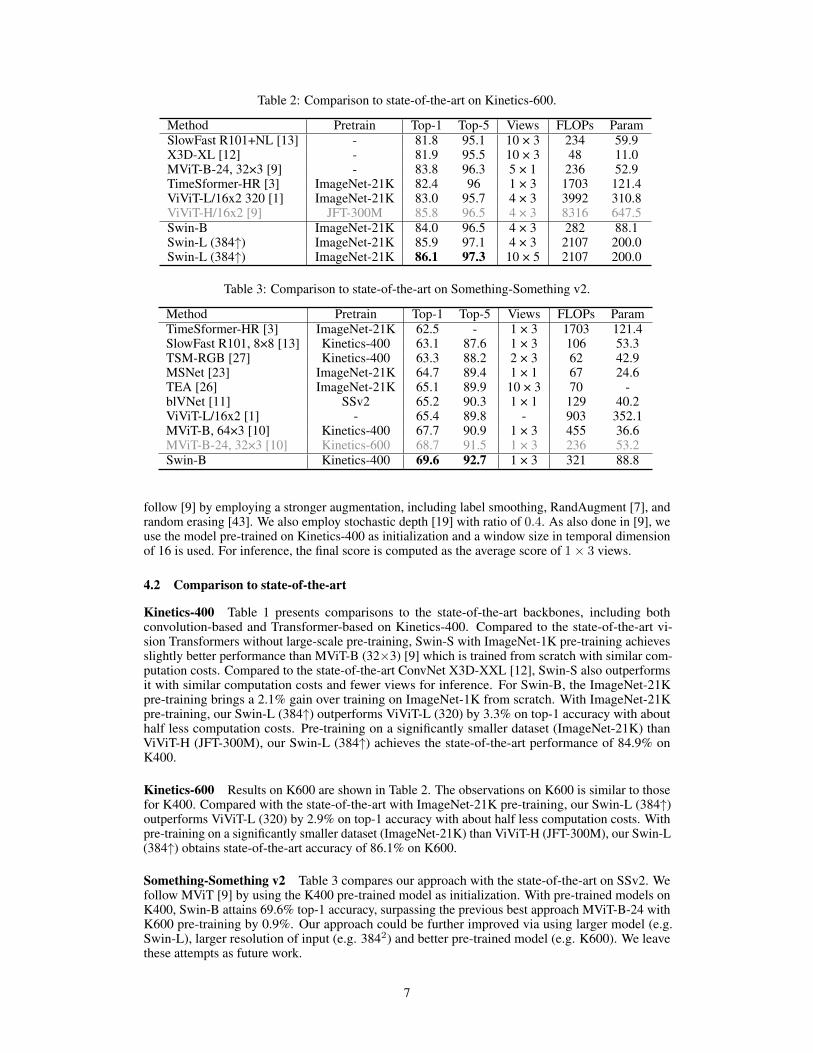
Table 2: Comparison to state-of-the-art on Kinetics-600.
follow [9] by employing a stronger augmentation, including label smoothing, RandAugment [7], andrandom erasing [43]. We also employ stochastic depth [19] with ratio of 0.4. As also done in [9], weuse the model pre-trained on Kinetics-400 as initialization and a window size in temporal dimensionof 16 is used. For inference, the final score is computed as the average score of 1× 3 views.
4.2 Comparison to state-of-the-art
Kinetics-400 Table 1 presents comparisons to the state-of-the-art backbones, including bothconvolution-based and Transformer-based on Kinetics-400. Compared to the state-of-the-art vi-sion Transformers without large-scale pre-training, Swin-S with ImageNet-1K pre-training achievesslightly better performance than MViT-B (32×3) [9] which is trained from scratch with similar com-putation costs. Compared to the state-of-the-art ConvNet X3D-XXL [12], Swin-S also outperformsit with similar computation costs and fewer views for inference. For Swin-B, the ImageNet-21Kpre-training brings a 2.1% gain over training on ImageNet-1K from scratch. With ImageNet-21Kpre-training, our Swin-L (384↑) outperforms ViViT-L (320) by 3.3% on top-1 accuracy with abouthalf less computation costs. Pre-training on a significantly smaller dataset (ImageNet-21K) thanViViT-H (JFT-300M), our Swin-L (384↑) achieves the state-of-the-art performance of 84.9% onK400.
Kinetics-600 Results on K600 are shown in Table 2. The observations on K600 is similar to thosefor K400. Compared with the state-of-the-art with ImageNet-21K pre-training, our Swin-L (384↑)outperforms ViViT-L (320) by 2.9% on top-1 accuracy with about half less computation costs. Withpre-training on a significantly smaller dataset (ImageNet-21K) than ViViT-H (JFT-300M), our Swin-L(384↑) obtains state-of-the-art accuracy of 86.1% on K600.
Something-Something v2 Table 3 compares our approach with the state-of-the-art on SSv2. Wefollow MViT [9] by using the K400 pre-trained model as initialization. With pre-trained models onK400, Swin-B attains 69.6% top-1 accuracy, surpassing the previous best approach MViT-B-24 withK600 pre-training by 0.9%. Our approach could be further improved via using larger model (e.g.Swin-L), larger resolution of input (e.g. 3842) and better pre-trained model (e.g. K600). We leavethese attempts as future work.
7
4.3 Ablation Study
Different designs for spatiotemporal attention We ablate three major designs for spatiotemporalattention: joint, split and factorized variants. The joint version jointly computes spatiotemporalattention in each 3D window-based MSA layer, which is our default setting. The split version addstwo temporal transformer layers on top of the spatial-only Swin Transformer, which is shown to beeffective in ViViT [1] and VTN [29]. The factorized version adds a temporal-only MSA layer aftereach spatial-only MSA layer in Swin Transformer, which is found to be effective in TimeSformer [3].For the factorized version, to reduce the bad effects of adding randomly initialized layers into thebackbone with pre-trained weights, we add a weighting parameter at the end of each temporal-onlyMSA layer which is initialized as zero.
Table 4: Ablation study on different designs for spatiotemporal attention with Swin-T on K400.
Results are shown in Table 4. We can observe that the joint version achieves the best speed-accuracytradeoff. This is mainly because locality in the spatial domain reduces computation for the jointversion while maintaining effectiveness. In contrast, a joint version based on ViT/DeiT would betoo computationally expensive. The split version does not work well in our scenarios. Though thisversion could naturally benefit from the pre-trained model, the temporal modeling of this version isnot as efficient. The factorized version yields relatively high top-1 accuracy but requires many moreparameters than the joint version. This is due the factorized version having a temporal-only attentionlayer after each spatial-only attention layer, while the joint version performs spatial and temporalattention in the same attention layer.
Table 5: Ablation study on temporal dimension of 3D tokens and temporal window size with Swin-Ton K400.
Temporal dimension of 3D tokens We perform an ablation study on the temporal dimension of3D tokens in a temporally global fashion, where the temporal dimension of 3D tokens is equal tothe temporal window size. Results with Swin-T on K400 are shown in Table 5. In general, a largertemporal dimension leads to a higher top-1 accuracy but with greater computation costs and slowerinference.
Temporal window size Fixing the temporal dimension of 3D tokens to 16, we perform an ablationstudy over temporal window sizes of 4/8/16. Results with Swin-T on K400 are shown in Table 5. Weobserve that Swin-T with a temporal window size of 8 incurs only a small performance drop of 0.3compared to a temporal window size of 16 (temporally global), but with a 17% relative decrease incomputation (88 vs. 106). This indicates that temporal locality brings an improved speed-accuracytradeoff for video recognition. If the number of input frames is extremely large, temporal localitywould have an even greater impact.
3D shifted windows Ablations of the 3D shifted windowing approach on Swin-T are reported forK400 in Table 6. 3D shifted windows bring +0.7% in top-1 accuracy, and temporally shifted windowsyield +0.3%. The results indicate the effectiveness of the 3D shifted windowing scheme to buildconnections among non-overlapping windows.
8
Table 6: Ablation study on the 3D shifted window approach with Swin-T on K400.
Top-1 Top-5w. 3D shifting 78.8 93.6w/o temporal shifting 78.5 93.5w/o 3D shifting 78.1 93.3
Ratio of backbone/head learning rate An interesting finding on the ratio of backbone and headlearning rates is shown in Table 7. With a model pre-trained on ImageNet-1K/ImageNet-21K, weobserve that a lower learning rate of the backbone architecture (e.g. 0.1×) relative to that of thehead, which is randomly initialized, brings gains in top-1 accuracy for K400. Also, using the modelpre-trained on ImageNet-21K benefits more from this technique, due to the model pre-trained onImageNet-21K being stronger. As a result, the backbone forgets the pre-trained parameters and dataslowly while fitting the new video input, leading to better generalization. This observation suggests adirection for further study on how to better utilize pre-trained weights.
Table 7: Ablation study on the ratio of backbone lr and head lr with Swin-B on K400.
Initialization on linear embedding layer and 3D relative position bias matrix In ViViT [1],center initialization of the linear embedding layer outperforms inflate initialization by a large margin.This motivates us to conduct an ablation study on these two initialization methods for Video SwinTransformer. As shown in Table 8, we surprisingly find that Swin-T with center initializationobtains the same performance as Swin-T with inflate initialization, of 78.8% top-1 accuracy usingthe ImageNet-1K pre-trained model2 On K400. In this paper, we adopt the conventional inflateinitialization on the linear embedding layer by default.
Table 8: Ablation study on the two initializa-tion methods of linear embedding layer withSwin-T on K400.
Initialization Top 1 Top 5Inflate 78.8 93.6Center 78.8 93.7
Table 9: Ablation study on the two initial-ization methods of 3D relative position biasmatrix with Swin-T on K400.
Initialization Top 1 Top 5Duplicate 78.8 93.6Center 78.8 93.6
For the 3D relative position bias matrix, we also have two different initialization choices, duplicate orcenter initialization. Unlike the center initialization method for linear embedding layer, we initializethe 3D relative position bias matrix by masking the relative position bias across different frameswith a small negative value (e.g. -4.6), so that each token only focuses inside the same frame fromthe very beginning. As shown in Table 9, we find that both initialization methods achieve the sametop-1 accuracy of 78.8% with Swin-T on K400. We adopt duplicate initialization on the 3D RelativePosition Bias matrix by default.
5 Conclusion
We presented a pure-transformer architecture for video recognition that is based on spatiotemporallocality inductive bias. This model is adapted from the Swin Transformer for image recognition, andthus it could leverage the power of the strong pre-trained image models. The proposed approachachieves state-of-the-art performance on three widely-used benchmarks, Kinetics-400, Kinetics-600and Something-Something v2. We made the code publicly available to facilitate future study in thisfield.
2As this observation is inconsistent with that in [1], we will analyze the difference once the code of ViViT isreleased.
9
References[1] Arnab, A., Dehghani, M., Heigold, G., Sun, C., Lucic, M., and Schmid, C. (2021). Vivit: A video
[2] Bao, H., Dong, L., Wei, F., Wang, W., Yang, N., Liu, X., Wang, Y., Gao, J., Piao, S., Zhou, M.,et al. (2020). Unilmv2: Pseudo-masked language models for unified language model pre-training.In International Conference on Machine Learning, pages 642–652. PMLR.
[3] Bertasius, G., Wang, H., and Torresani, L. (2021). Is space-time attention all you need for videounderstanding? arXiv preprint arXiv:2102.05095.
[4] Cao, Y., Xu, J., Lin, S., Wei, F., and Hu, H. (2019). Gcnet: Non-local networks meet squeeze-excitation networks and beyond. In Proceedings of the IEEE/CVF International Conference onComputer Vision (ICCV) Workshops.
[5] Carreira, J. and Zisserman, A. (2017a). Quo vadis, action recognition? a new model andthe kinetics dataset. In proceedings of the IEEE Conference on Computer Vision and PatternRecognition, pages 6299–6308.
[6] Carreira, J. and Zisserman, A. (2017b). Quo vadis, action recognition? a new model andthe kinetics dataset. In proceedings of the IEEE Conference on Computer Vision and PatternRecognition, pages 6299–6308.
[7] Cubuk, E. D., Zoph, B., Shlens, J., and Le, Q. V. (2020). Randaugment: Practical automateddata augmentation with a reduced search space. In Proceedings of the IEEE/CVF Conference onComputer Vision and Pattern Recognition Workshops, pages 702–703.
[8] Dosovitskiy, A., Beyer, L., Kolesnikov, A., Weissenborn, D., Zhai, X., Unterthiner, T., Dehghani,M., Minderer, M., Heigold, G., Gelly, S., Uszkoreit, J., and Houlsby, N. (2021). An image isworth 16x16 words: Transformers for image recognition at scale. In International Conference onLearning Representations.
[9] Fan, H., Xiong, B., Mangalam, K., Li, Y., Yan, Z., Malik, J., and Feichtenhofer, C. (2021a).Multiscale vision transformers. arXiv:2104.11227.
[10] Fan, H., Xiong, B., Mangalam, K., Li, Y., Yan, Z., Malik, J., and Feichtenhofer, C. (2021b).Multiscale vision transformers. arXiv preprint arXiv:2104.11227.
[11] Fan, Q., Chen, C.-F., Kuehne, H., Pistoia, M., and Cox, D. (2019). More is less: Learningefficient video representations by big-little network and depthwise temporal aggregation. arXivpreprint arXiv:1912.00869.
[12] Feichtenhofer, C. (2020). X3d: Expanding architectures for efficient video recognition. InProceedings of the IEEE/CVF Conference on Computer Vision and Pattern Recognition, pages203–213.
[13] Feichtenhofer, C., Fan, H., Malik, J., and He, K. (2019). Slowfast networks for video recognition.In Proceedings of the IEEE/CVF International Conference on Computer Vision, pages 6202–6211.
[14] Goyal, R., Ebrahimi Kahou, S., Michalski, V., Materzynska, J., Westphal, S., Kim, H., Haenel,V., Fruend, I., Yianilos, P., Mueller-Freitag, M., et al. (2017). The" something something"video database for learning and evaluating visual common sense. In Proceedings of the IEEEInternational Conference on Computer Vision, pages 5842–5850.
[15] He, K., Zhang, X., Ren, S., and Sun, J. (2016). Deep residual learning for image recognition. InProceedings of the IEEE conference on computer vision and pattern recognition, pages 770–778.
[16] Hu, H., Gu, J., Zhang, Z., Dai, J., and Wei, Y. (2018). Relation networks for object detection.In Proceedings of the IEEE Conference on Computer Vision and Pattern Recognition, pages3588–3597.
[17] Hu, H., Zhang, Z., Xie, Z., and Lin, S. (2019). Local relation networks for image recognition.In Proceedings of the IEEE/CVF International Conference on Computer Vision (ICCV), pages3464–3473.
10
[18] Huang, G., Liu, Z., Van Der Maaten, L., and Weinberger, K. Q. (2017). Densely connectedconvolutional networks. In Proceedings of the IEEE conference on computer vision and patternrecognition, pages 4700–4708.
[19] Huang, G., Sun, Y., Liu, Z., Sedra, D., and Weinberger, K. Q. (2016). Deep networks withstochastic depth. In European conference on computer vision, pages 646–661. Springer.
[20] Kay, W., Carreira, J., Simonyan, K., Zhang, B., Hillier, C., Vijayanarasimhan, S., Viola, F.,Green, T., Back, T., Natsev, P., et al. (2017). The kinetics human action video dataset. arXivpreprint arXiv:1705.06950.
[21] Kingma, D. P. and Ba, J. (2014). Adam: A method for stochastic optimization. arXiv preprintarXiv:1412.6980.
[22] Krizhevsky, A., Sutskever, I., and Hinton, G. E. (2012). Imagenet classification with deepconvolutional neural networks. In Advances in neural information processing systems, pages1097–1105.
[23] Kwon, H., Kim, M., Kwak, S., and Cho, M. (2020). Motionsqueeze: Neural motion featurelearning for video understanding. In European Conference on Computer Vision, pages 345–362.Springer.
[24] LeCun, Y., Bottou, L., Bengio, Y., Haffner, P., et al. (1998). Gradient-based learning applied todocument recognition. Proceedings of the IEEE, 86(11):2278–2324.
[25] Li, X., Zhang, Y., Liu, C., Shuai, B., Zhu, Y., Brattoli, B., Chen, H., Marsic, I., and Tighe, J.(2021). Vidtr: Video transformer without convolutions. arXiv preprint arXiv:2104.11746.
[26] Li, Y., Ji, B., Shi, X., Zhang, J., Kang, B., and Wang, L. (2020). Tea: Temporal excitation andaggregation for action recognition. In Proceedings of the IEEE/CVF Conference on ComputerVision and Pattern Recognition, pages 909–918.
[27] Lin, J., Gan, C., and Han, S. (2019). Tsm: Temporal shift module for efficient video under-standing. In Proceedings of the IEEE/CVF International Conference on Computer Vision, pages7083–7093.
[28] Liu, Z., Lin, Y., Cao, Y., Hu, H., Wei, Y., Zhang, Z., Lin, S., and Guo, B. (2021). Swin trans-former: Hierarchical vision transformer using shifted windows. arXiv preprint arXiv:2103.14030.
[29] Neimark, D., Bar, O., Zohar, M., and Asselmann, D. (2021). Video transformer network. arXivpreprint arXiv:2102.00719.
[30] Qiu, Z., Yao, T., and Mei, T. (2017). Learning spatio-temporal representation with pseudo-3dresidual networks. In proceedings of the IEEE International Conference on Computer Vision,pages 5533–5541.
[31] Raffel, C., Shazeer, N., Roberts, A., Lee, K., Narang, S., Matena, M., Zhou, Y., Li, W., andLiu, P. J. (2020). Exploring the limits of transfer learning with a unified text-to-text transformer.Journal of Machine Learning Research, 21(140):1–67.
[32] Simonyan, K. and Zisserman, A. (2015). Very deep convolutional networks for large-scaleimage recognition. In International Conference on Learning Representations.
[33] Szegedy, C., Liu, W., Jia, Y., Sermanet, P., Reed, S., Anguelov, D., Erhan, D., Vanhoucke,V., and Rabinovich, A. (2015). Going deeper with convolutions. In Proceedings of the IEEEconference on computer vision and pattern recognition, pages 1–9.
[34] Touvron, H., Cord, M., Douze, M., Massa, F., Sablayrolles, A., and Jégou, H. (2020).Training data-efficient image transformers & distillation through attention. arXiv preprintarXiv:2012.12877.
[35] Tran, D., Bourdev, L., Fergus, R., Torresani, L., and Paluri, M. (2015). Learning spatiotemporalfeatures with 3d convolutional networks. In Proceedings of the IEEE international conference oncomputer vision, pages 4489–4497.
11
[36] Tran, D., Wang, H., Torresani, L., and Feiszli, M. (2019). Video classification with channel-separated convolutional networks. In Proceedings of the IEEE/CVF International Conference onComputer Vision, pages 5552–5561.
[37] Tran, D., Wang, H., Torresani, L., Ray, J., LeCun, Y., and Paluri, M. (2018). A closer look atspatiotemporal convolutions for action recognition. In Proceedings of the IEEE conference onComputer Vision and Pattern Recognition, pages 6450–6459.
[38] Vaswani, A., Shazeer, N., Parmar, N., Uszkoreit, J., Jones, L., Gomez, A. N., Kaiser, Ł., andPolosukhin, I. (2017). Attention is all you need. In Advances in Neural Information ProcessingSystems, pages 5998–6008.
[39] Wang, H., Tran, D., Torresani, L., and Feiszli, M. (2020). Video modeling with correlation net-works. In Proceedings of the IEEE/CVF Conference on Computer Vision and Pattern Recognition,pages 352–361.
[40] Wang, X., Girshick, R., Gupta, A., and He, K. (2018). Non-local neural networks. In Proceed-ings of the IEEE conference on computer vision and pattern recognition, pages 7794–7803.
[41] Xie, S., Sun, C., Huang, J., Tu, Z., and Murphy, K. (2018). Rethinking spatiotemporal featurelearning: Speed-accuracy trade-offs in video classification. In Proceedings of the EuropeanConference on Computer Vision (ECCV), pages 305–321.
[42] Yin, M., Yao, Z., Cao, Y., Li, X., Zhang, Z., Lin, S., and Hu, H. (2020). Disentangled non-localneural networks. In Proceedings of the European conference on computer vision (ECCV).
[43] Zhong, Z., Zheng, L., Kang, G., Li, S., and Yang, Y. (2020). Random erasing data augmentation.In Proceedings of the AAAI Conference on Artificial Intelligence, volume 34, pages 13001–13008.