1 New York City College of Technology Of The City University Of New York Electrical and Telecommunications Engineering Technology Department Sensors and Instruments Course: EET 3120 Section: E260 Experiment 2: Graphical Programming in Lab VIEW Name Busayo Daramola Michaelangelo D. Brown Zeeshan Ahmed
Transcript
1
New York City College of Technology Of The City University Of New York
Electrical and Telecommunications Engineering Technology Department
This lab introduces the idea of a computer graphical programming instrument in the LabVIEW
through building a simple instrument by using some tools from function palette workstation and
controlling it with a LabVIEW program. The lab also gives a short tutorial for LabVIEW
graphical programming and also to wire the circuit into LabVIEW to see how it works
Equipment Desk-top computer
LabVIEW software
Theoretical Background
LabVIEW ties the creation of user interfaces (called front panels) into the development cycle.
LabVIEW programs/subroutines are called virtual instruments (VIs). Each VI has three
components: a block diagram, a front panel and a connector panel. The last is used to represent
the VI in the block diagrams of other, calling VIs. The front panel is built using controls and
indicators. Controls are inputs – they allow a user to supply information to the VI. Indicators are
outputs – they indicate, or display, the results based on the inputs given to the VI. The back
panel, which is a block diagram, contains the graphical source code. All of the objects placed on
the front panel will appear on the back panel as terminals. The back panel also contains
structures and functions which perform operations on controls and supply data to indicators. The
structures and functions are found on the Functions palette and can be placed on the back panel.
Collectively controls, indicators, structures and functions will be referred to as nodes. Nodes are
connected to one another using wires – e.g. two controls and an indicator can be wired to the
4
addition function so that the indicator displays the sum of the two controls. Thus a virtual
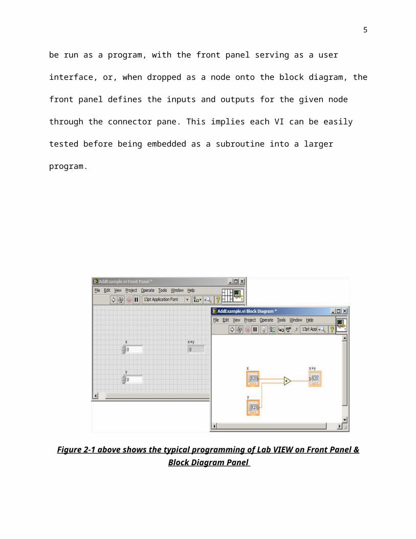
instrument can either be run as a program, with the front panel serving as a user interface, or,
when dropped as a node onto the block diagram, the front panel defines the inputs and outputs
for the given node through the connector pane. This implies each VI can be easily tested before
being embedded as a subroutine into a larger program.
Figure 2-1 above shows the typical programming of Lab VIEW on Front Panel & Block Diagram Panel
5
PROCEDURE
The Voltage.vi
For the first part of the experiment we created a simulation of a voltage ranging from 4.2
to 10. A random number generator was used to generate a number between 0 and 1. This number
was then multiplied by 0.1 and added to 4.2 which resulted in a number in the range of 4.2 to 10.
To build this voltage simulator, the following steps were performed:
1. A Meter indicator was moved from Express>>Numeric Indicators in the Controls Palette
and placed on a blank Panel. It was labeled Voltage. This is shown in Figure 2-2.
2. A Random Number (0-1) function was placed in the Diagram window from the Function
Palette.
3. From Express>>Arithmetic& Comparison>>Express Numeric in the Function Palette,
one multiply function, one Add function, and two Numeric Constant functions were
placed in the Diagram window. The Numeric Constants were given the values 4.2 and
0.1.
4. The connections were made as shown in Figure 2-2.
6
Experimental results:
The Voltage. Vi
This results shows that we have a temperature sensor that gives out voltage that is proportional with the temperature on the Celsius scale by using following equation:
7
Figure 2-2: The Panel and Diagram for the Voltage.vi
Kelvin
Celsius
Fahrenheit
Figure 2-3: Connection of the Fahrenheit case structure
8
Figure 2-4: Connection of the Celsius case structure
9
Figure 2-5: Connection of the Kelvin case structure
Figure 2-6: Editing the Connector
10
V=R∗a+bRandom No. a b Voltage
1 0.4 2.9 2.91 0.5 4 4.21 0.6 4.5 4.9
Figure 2-7: Shows V=R∗a+b = 4.9
V=1∗0.6+4.5 = 4.9
t [ K ]=U [ V ]∗a
Voltage a K05 100 501 100 100
1.5 100 250
Figure 2-8: Shows K=V∗a = 100
V=1∗100 = 100
11
t [℃ ]=U [V ]∗a−273.15
Voltage a b Celsius1 100 273.15 -73.152 100 273.15 -73.153 100 273.15 -73.15
Figure 2-9: Shows
C=V∗a-273.15 = -73.15
C=2∗100−273.15 = -73.15
Conclusion
This experiment introduces my knowledge in the LABVEIW graphical programming son how I
can manipulate and use the LabVIEW to see the relationship between voltage and temperature.
Also, it showed me how to represent the voltage-temperature relationship on the lab view
through graphical representation.
Reference
EET 3120 Sensors and Instruments Laboratory Manual by Professor Viviana Vladutescu, Spring 2015.