View/Open - Oregon State University

AN ABSTRACT OF THE THESIS OF

Andrew W. Strahler for the degree of Master of Science in Civil Engineering

presented on March 14, 2012.

Title: Bearing Capacity and Immediate Settlement of Shallow Foundation on

Clay.

Abstract approved:

Armin W. Stuedlein

Shallow foundations are extensively used to support structures of all

sizes and derive their support from near surface soils. Thus, they are typically

embedded up to a few meters into the soil profile. Designers of shallow

foundations are required to meet two limit states: overall failure of the soil

beneath the foundation (bearing capacity) and excessive settlement. Existing

bearing capacity design methods use an assumed shearing plane within the soil

and perfectly plastic soil behavior to estimate the ultimate resistance available.

The immediate settlement of a shallow foundation is typically approximated

using an elasticity-based method that does not account for actual, nonlinear

soil behavior. A load test database was developed from footing load tests

reported in the literature to assess the accuracy and uncertainty in existing

design methodologies for calculating bearing capacity and immediate

settlement. The assessment of uncertainty in bearing capacity and immediate

settlement was accomplished through the application of a hyperbolic bearing

pressure-displacement model, and the adaptation of the Duncan-Chang soil

constitutive model to footing displacements.

The prediction of bearing capacity using the general bearing capacity

formula was compared to the bearing capacity extrapolated from the load test

database using a hyperbolic bearing pressure-displacement model. On average

the general bearing capacity formula under-predicts the bearing capacity and

exhibits a significant amount of variability. The comparison was used to

develop resistance statistics that were implemented to produce resistance

factors for an LRFD based design approach using AASHTO load statistics.

The Duncan-Chang model was adapted to predict bearing pressure-

displacement curves for footings in the load test database and used to estimate

governing soil parameters. Bearing pressure-displacement curves fitted to the

observed curves were used to back calculate soil stiffness. The soil stiffness

was used with an elasticity-based displacement prediction method to evaluate

the accuracy of the method. Finally, the back-calculated modulus from the

fitted Duncan-Chang model was used to assess the accuracy and uncertainty

associated with the elasticity-based K-factor, a correlation based stiffness

parameter. In general the comparisons indicate that the current design

procedures over-predict the bearing pressure associated with a given

displacement and exhibit a significant amount of uncertainty.

© Copyright by Andrew W. Strahler

March 14, 2012

All Rights Reserved

Bearing Capacity and Immediate Settlement of Shallow Foundations on Clay

by

Andrew W. Strahler

A THESIS

submitted to

Oregon State University

in partial fulfillment of

the requirements for the

degree of

Master of Science

Presented March 14, 2012

Commencement June 2012

Master of Science thesis of Andrew W. Strahler presented on March 14, 2012.

APPROVED:

Major Professor, representing Civil Engineering

Head of the School of Civil and Construction Engineering

Dean of the Graduate School

I understand that my thesis will become part of the permanent collection of

Oregon State University libraries. My signature below authorizes release of my

thesis to any reader upon request.

Andrew W. Strahler, Author

ACKNOWLEDGEMENTS

I would like to first and foremost thank my graduate advisor, Professor

Armin Stuedlein. The completion of this document would not have been

possible without his dedication and due diligence. He has guided me in more

ways than I can count and his patience and support gave me the strength to

push through the hard times.

I am also very grateful for the support and comments provided by my

graduate thesis committee: Professors Edward Dever, Ben Mason and Michael

Olsen. I would also like to thank my friends and family. Their help and

encouragement propelled me to endure this effort. I would also like to thank

the School of Civil and Construction Engineering for their support and

guidance.

TABLE OF CONTENTS

Page

Chapter 1: Introduction ..................................................................................... 1

1.1. Statement of Problem ......................................................................... 1

1.2. Purpose and Scope .............................................................................. 2

1.3. Outline ................................................................................................ 2

Chapter 2: Review of Literature on Immediate Settlement of Shallow

Foundations on Clay ............................................................................... 5

2.1. Introduction ........................................................................................ 5

2.2. Bearing Capacity of Shallow Foundations ......................................... 6

2.2.1. Generalized Bearing Capacity Theory ........................................... 6

2.2.2. Evaluation of Bearing Capacity from Load Test Data ................. 13

2.3. Settlement ......................................................................................... 16

2.3.1. Total Settlement ........................................................................... 17

2.3.2. Distortion Settlement ................................................................... 18

2.4. Selected Aspects of Cohesive Soil Behavior .................................... 19

2.4.1. Stress history ................................................................................ 20

2.4.2. Strain Rate .................................................................................... 21

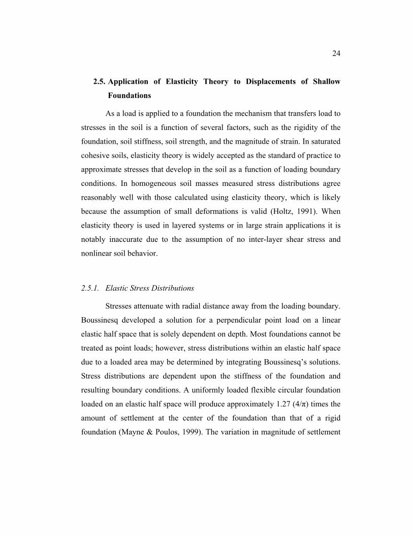
2.5. Application of Elasticity Theory to Displacements of Shallow Foundations ...................................................................................... 24

2.5.1. Elastic Stress Distributions .......................................................... 24

2.5.2. Elasticity-based Distortion Settlement ......................................... 27

2.5.3. Finite Element Analysis-based Approach .................................... 31

TABLE OF CONTENTS (continued)

Page

2.5.4. Use and Limitations of Young’s Modulus in Displacement

Estimation .................................................................................... 34

2.6. Nonlinear Distortion Displacement Models ..................................... 37

2.6.1. Mobilisable Strength Design (MSD) ........................................... 38

2.6.2. Small Strain Stiffness ................................................................... 39

2.6.3. Nonlinear Elastic Perfectly Plastic Soil Behavior Models ........... 41

2.7. Summary of Literature Review ........................................................ 45

Chapter 3: Research Objectives and Program ................................................. 46

3.1. Objectives of this Study .................................................................... 46

3.2. Research Program ............................................................................. 46

Chapter 4: Database of Loading Test Case Histories ...................................... 50

4.1. Introduction ...................................................................................... 50

4.2. Criteria and Selection of Case Histories ........................................... 50

4.3. Case History Index and Overview .................................................... 52

4.3.1. Bangkok, Thailand - 1972 ............................................................ 52

4.3.2. Glasgow, Scotland - 1975 ............................................................ 57

4.3.3. Corvallis, Oregon, U.S.A. - 1975 ................................................. 57

4.3.4. Ottawa, Canada - 1976 ................................................................. 58

4.3.5. Cowden, England - 1980 .............................................................. 58

4.3.6. Haga, Norway - 1982 ................................................................... 59

4.3.7. Bangkok, Thailand - 1984 ............................................................ 59

4.3.8. Alvin, Texas, U.S.A. - 1986 ......................................................... 60

4.3.9. Bothkennar, Scotland - 1993 ........................................................ 60


Page

4.3.10. Bombay, India - 1994 ................................................................... 61

4.3.11. Belfast, Ireland - 2003 .................................................................. 61

4.3.12. Baytown, Texas, U.S.A. - 2010 ................................................... 62

4.4. Summary of Loading Test Database ................................................ 62

Chapter 5: Development of Load Test Database and Methodology ............... 63

5.1. Introduction ...................................................................................... 63

5.2. General Statistical Approach ............................................................ 64

5.3. Development of Soil Profiles ........................................................... 66

5.4. Estimation of Selected Soil Parameters ............................................ 67

5.4.1. Undrained Shear Strength ............................................................ 67

5.4.2. Overconsolidation Ratio .............................................................. 70

5.4.3. Initial Undrained Young’s Modulus ............................................ 72

5.5. Load Test Database .......................................................................... 73

5.6. Summary of Methodology ................................................................ 76

Chapter 6: Uncertainty in Prediction of Bearing Capacity .............................. 77

6.1. Introduction ...................................................................................... 77

6.2. Application and Uncertainty of the Hyperbolic Model to Bearing Pressure-Displacement Curves ......................................................... 77

6.3. Uncertainty in Bearing Capacity using Estimated Undrained Shear Strengths ........................................................................................... 85

6.3.1. Bearing Capacity Predicted Using Estimated Undrained Shear

Strengths ....................................................................................... 86


Page

6.3.2. Effects of Surcharge on Bearing Capacity ................................... 87

6.3.3. Evaluating Predicted Bearing Capacity for Dependency ............. 89

6.3.4. Effect of Undrained Shear Strength on Prediction of Bearing

Capacity using Monte Carlo Simulation ...................................... 90

6.4. Back-Calculation of Undrained Shear Strength using the Hyperbolic Model ................................................................................................ 96

6.5. Summary ......................................................................................... 100

Chapter 7: Uncertainty in Prediction of Displacements ................................ 102

7.1. Introduction .................................................................................... 102

7.2. Development of Proposed Model ................................................... 102

7.3. Application and Validity of the Duncan-Chang Model .................. 106

7.4. Results of Model Application ......................................................... 111

7.4.1. Bearing Pressure-Displacement Curves Using Estimated Stiffness

Parameters (Case 1).................................................................... 112

7.4.2. Back calculation of the Initial Undrained Young’s Modulus (Case

2) ................................................................................................ 116

7.4.3. Elasticity-Based Displacement Prediction (Case 3) ................... 122

7.4.4. Back-calculation of the K-factor (Case 4) ................................. 128

7.5. Summary ......................................................................................... 131

Chapter 8: Calibration of Resistance Factors for the Bearing Capacity

Model .................................................................................................. 133

8.1. Introduction .................................................................................... 133

8.2. Limit State Design .......................................................................... 134


Page

8.3. Statistical Characterization of Resistance Distribution .................. 138

8.4. Resistance Factor Calibration using the Monte Carlo Approach ... 142

8.5. Target Reliability Indices and Calculation of Load and Resistance Factors ............................................................................................ 144

8.6. Summary ......................................................................................... 146

Chapter 9: Summary and Conclusions .......................................................... 147

9.1. Summary ......................................................................................... 147

9.2. Conclusions .................................................................................... 148

9.2.1. Uncertainty in Bearing Capacity Predictions ............................. 148

9.2.2. Uncertainty in Prediction of Bearing Pressure-Displacement ... 149

9.2.3. Proposed Model for Bearing Capacity Prediction ..................... 150

Bibliography .................................................................................................... 152

Appendix A: Soil Profile Database ................................................................. 162

Case History: Bangkok, Thailand - 1972 (Brand, et al., 1972) ................. 163

Case History: Corvallis, Oregon, U.S.A. - 1975 (Newton, 1975) ............ 166

Case History: Ottawa, Canada - 1976 (Bauer, et al., 1976) ...................... 167

Case History: Cowden, England - 1980 (Marsland & Powell, 1980) ....... 168

Case History: Haga, Norway - 1982 (Andersen & Stenhamer, 1982) ...... 169

Case History: Bangkok, Thailand - 1984 (Bergado, et al., 1984) ............. 171

Case History: Alvin, Texas, U.S.A. - 1986 (Tand & Funegard, 1986) ..... 173

Case History: Bothkennar, Scotland - 1993 (Jardine, 1993) ..................... 179


Page

Case History: Belfast, Ireland - 2003 (Lehane, 2003) .............................. 182

Case History: Baytown, Texas, U.S.A. - 2010 (Stuedlein & Holtz, 2010)183

Appendix B: Bearing Pressure-Displacement and Transformed Curves ........ 184

LIST OF FIGURES

Figure Page

Figure 2.2.1. Bearing capacity failure surface in clay......................................... 7

Figure 2.2.2. Bearing capacity failure mechanisms, modified after (Vesic, 1973). ...................................................................................................... 8

Figure 2.2.3. Typical bearing pressure-displacement curves after (Brand, et al., 1972) ..................................................................................................... 14

Figure 2.2.4. Example of Chin load-displacement transformation with data from Figure 2.2.3. ................................................................................. 16

Figure 2.4.1 Normalized undrained shear strength vs. strain rate for re-sedimented Boston Blue Clay after (Sheahan, et al., 1996). ................. 23

Figure 2.5.1. Contact pressures for varying soil and footing rigidity type, from (Holtz, 1991). ........................................................................................ 27

Figure 2.5.2. Linear elastic-perfectly plastic soil behavior. .............................. 28

Figure 2.5.3. Stress distributions in an elastic layer, after (Carrier & Christian, 1978). .................................................................................................... 29

Figure 2.5.4. Burland’s effect of embedment, from (Burland, 1970). .............. 30

Figure 2.5.5. Settlement ratio with applied stress ratio, from (D'Appolonia, et al., 1971). .............................................................................................. 33

Figure 2.5.6. Observed full scale footing displacements compared to displacements predicted after the method of D’Appolonia et al. (1971): (a) large 2.74 m square footing; (b) small 0.76 m circular footing, from (Stuedlein & Holtz, 2010). .................................................................... 34

Figure 2.5.7. Linear elastic vs. nonlinear stress strain behavior. ...................... 35

Figure 2.5.8. Various types of elastic moduli. .................................................. 36

Figure 2.5.9. Variation in K-factor based on OCR and PI, from (Duncan & Buchignani, 1987). ................................................................................ 37

Figure 2.6.1. Illustration of the MSD approach, after (Osman, et al., 2007). ... 39

LIST OF FIGURES (continued)

Figure Page

Figure 2.6.2. Comparison of predicted Elhakim and Mayne q-δ vs. Observed, data from Stuedlein et al. (2010). .......................................................... 41

Figure 2.6.3. Influence factors for distortion settlement, after (Foye, et al., 2008); (a) strip footings; (b) square footings; and (c) rectangular (L/B=2) footings ................................................................................... 43

Figure 2.6.4. (a) Iq computed from soil parameters at the base of a typical footing and (b) Iq computed from average soil parameters (Foye, et al., 2008). .................................................................................................... 43

Figure 2.6.5. Comparison of Foye et al. (2008) method with observed data (Stuedlein & Holtz, 2010) ..................................................................... 44

Figure 3.2.1. Development of soil profiles and bearing capacity model based on the application of the hyperbolic model to q-δ curves. .................... 48

Figure 3.2.2. Flow chart of the research program for the assessment of the Duncan-Chang model. .......................................................................... 49

Figure 5.1.1. Uncertainty in soil property estimates (Kulhawy, 1992). ............ 64

Figure 5.2.1. Conceptual visualization of the defined bias assuming a normal distribution. ........................................................................................... 66

Figure 5.4.1. VST correction factor based on PI, after (Kulhawy & Mayne, 1990). .................................................................................................... 69

Figure 5.4.2. Variation in K-factor based on OCR and PI, from (Duncan & Buchignani, 1987). ................................................................................ 73

Figure 6.2.1. Hyperbolic fitting method applied to footing load test TS-1. ...... 79

Figure 6.2.2. Fitted hyperbolic q-δ curve using method compared to that observed for footing load test TS-1. ...................................................... 80

Figure 6.2.3. Sample and fitted distributions of point biases for the observed and fitted bearing pressures and displacements. ................................... 83


Figure Page

Figure 6.2.4. Sample and fitted distributions of averaged biases for the observed and fitted bearing pressures and displacements. .................... 85

Figure 6.3.1. Sample and fitted distributions of the biases for the observed and predicted bearing capacity. ................................................................... 87

Figure 6.3.2. Traditional bearing capacity versus bearing capacity bias. ......... 90

Figure 6.3.3. CDFs of bearing capacity showing variations in undrained shear strength for Case A. .............................................................................. 94

Figure 6.3.4. CDFs of bearing capacity showing variations in undrained shear strength for Case B. ............................................................................... 95

Figure 6.3.5. Comparison of predicted bearing capacity CDFs at a COV of 30%. ...................................................................................................... 96

Figure 6.4.1. Example of mobilized undrained shear strength curve data for load test TS-1. ....................................................................................... 98

Figure 6.4.2. Distribution of undrained shear strength bias with fitted distributions. ........................................................................................ 100

Figure 7.2.1. Hyperbolic model stress-strain behavior. .................................. 104

Figure 7.2.2. Normalized elastic stress distributions beneath a rigid footing. 105

Figure 7.3.1. Predicted bearing pressure-displacement curve using Duncan-Chang model for load test TS-1. ......................................................... 109

Figure 7.3.2. Stresses beneath a footing calculated using the Duncan-Chang hyperbolic model for TS-1. ................................................................. 110

Figure 7.4.1. Predicted bearing pressure-displacement curve of Case 1a and 1b for load test TS-1. ............................................................................... 113

Figure 7.4.2. Distribution of biases for bearing pressure-displacement curves for Case 1a. ......................................................................................... 115


Figure Page

Figure 7.4.3. Distribution of biases for bearing pressure-displacement curves for Case 1b. ......................................................................................... 115

Figure 7.4.4. Back calculation of initial Young's modulus from Duncan-Chang model using bearing pressure-displacement curves for load test TS-1 (Case 2). .............................................................................................. 117

Figure 7.4.5. Distribution of biases for bearing pressure-displacement curves based on estimated su and back-calculated initial Young’s modulus. . 118

Figure 7.4.6. Distribution of biases for bearing pressure-displacement curves based on back-calculated su and back-calculated initial Young’s modulus. .............................................................................................. 119

Figure 7.4.7 Sample and fitted distributions for the initial Young’s modulus bias. ..................................................................................................... 122

Figure 7.4.8. Comparison of elasticity-based prediction displacement for load test TS-1. .............................................................................................. 123

Figure 7.4.9. Distribution of elasticity-based prediction biases for Case 3a at a displacement of 10 mm. ...................................................................... 125

Figure 7.4.10. Distribution of elasticity-based prediction biases calculated for Case 3b at displacement of 10 mm. .................................................... 126





Figure 7.4.15. Case 4a K-factor bias distribution with fitted distributions. .... 130


Figure Page

Figure 7.4.16. Case 4b K-factor bias distribution with fitted distributions..... 131

Figure 8.2.1. Conceptual illustration of potential probability density functions (PDFs) for load and resistance factors, from (Stuedlein, 2008). ......... 137

Figure 8.2.2. Conceptual illustration of a combined PDF representing the margin of safety and the reliability index, adapted from (Stuedlein, 2008). .................................................................................................. 138

Figure 8.3.1. CDF of standard normal variate as a function of bearing capacity prediction biases. ................................................................................. 140

Figure 8.5.1. Resistance factors for calculating bearing capacity without considering uncertainty in undrained shear strength. .......................... 145

LIST OF TABLES

Table Page

Table 2.2.1. Terzaghi bearing capacity approximations. .................................. 10

Table 2.2.2. Bearing capacity factors. ............................................................... 11

Table 2.2.3. Depth and shape factors. ............................................................... 12

Table 2.3.1. Potential for settlement component, adapted from (Holtz, 1991). 18

Table 4.3.1. Summary of full scale footing load tests. ...................................... 53

Table 5.4.1. Empirical OCR correlations used in statistical approach to estimate OCR profiles. .......................................................................... 70

Table 5.4.2. Statistical results of OCR comparison. ......................................... 71

Table 5.4.3. Expected ranges in saturated unit weight of clay soils based on OCR, from (Stuedlein, 2010) ................................................................ 72

Table 5.5.1. Summary of load test database of shallow footing on clay. .......... 75

Table 6.2.1. Statistical summary of biases for the fitting of the hyperbolic model to observed q-δ curves. ............................................................... 82

Table 6.3.1. Effect of surcharge on bearing capacity estimate. ........................ 88

Table 6.3.2. Monte Carlo simulations conducted to assess uncertainty. ........... 92

Table 6.3.3. Summary of bearing capacity distribution resulting from Case B Monte Carlo simulations. ...................................................................... 93

Table 6.3.4. Comparison of largest and smallest possible bearing capacities. . 94

Table 6.4.1. Summary of undrained shear strength comparison. .................... 100

Table 7.4.1. Summary of analysis methods and comparisons of the Duncan-Chang model. ...................................................................................... 111

LIST OF TABLES (continued)

Table Page

Table 7.4.2. Summary statistics of the Duncan-Chang model application to q-δ curves for Case 1a and 1b. .................................................................. 114

Table 7.4.3. Summary of the bias comparisons for Case 2a and Case 2b. ..... 117

Table 7.4.4. Summary of Case 2 using back-calculated undrained shear strength. ............................................................................................... 121

Table 7.4.5. Statistical summary of the analysis for Case 3. .......................... 124

Table 7.4.6. Summary of the statistical analysis of Case 4a and 4b. .............. 130

Table 8.3.1. Summary of theoretical distribution fitting of the bearing capacity bias distribution. .................................................................................. 139

Table 8.3.2. Final statistics of the adjusted fit-to-tail lognormal bearing capacity model. ................................................................................... 142

Table 8.4.1. Summary of AASHTO loading and bias statistics (Paikowsky, et al., 2004). ............................................................................................ 143

Table 9.2.1. Summary of statistical analyses presented in this study. ............ 151

LIST OF APPENDIX FIGURES

Figure Page

Figure A-1. Undrained shear strength profile for BB load tests in Bangkok, Thailand (Brand, et al., 1972). ........................................................... 163

Figure A-2. Moisture contents profile for BB load tests in Bangkok, Thailand (Brand, et al., 1972). ........................................................................... 164

Figure A-3. Vertical effect stress, preconsolidation stress and OCR profiles for BB load tests in Bangkok, Thailand (Moh, et al., 1969). .................... 165

Figure A-4. Moisture contents profile for ON load tests in Corvallis, Oregon (Newton, 1975). .................................................................................. 166

Figure A-5. Moisture contents, undrained shear strength and vertical stress profile for OB load tests in Ottawa, Canada (Bauer, et al., 1976). .... 167

Figure A-6. Moisture content and undrained shear strength profile for CM load tests in Cowden, England (Newton, 1975). ....................................... 168

Figure A-7. Moisture contents and undrained shear strength profile for HA load tests in Haga, Norway (Andersen & Stenhamer, 1982). ............ 169

Figure A-8. OCR profile for HA load tests in Haga, Norway (Andersen & Stenhamer, 1982). ............................................................................... 170

Figure A-9. OCR profile for RB load tests in Bangkok, Thailand (Bergado, et al., 1984). ............................................................................................ 171

Figure A-10. Vertical and preconsolidation stress profile for RB load tests in Bangkok, Thailand Invalid source specified.. ..................................... 172

Figure A-11. Cone tip resistance profile for TT load tests on site A in Alvin, Texas (Tand & Funegard, 1986). ....................................................... 173

Figure A-12. Moisture content, undrained shear strength and pressuremeter profiles for TT load tests on site A in Alvin, Texas (Tand & Funegard, 1986) ................................................................................................... 174

Figure A-13. Cone tip resistance profile for TT load tests on site B in Alvin, Texas (Tand & Funegard, 1986). ....................................................... 175

LIST OF APPENDIX FIGURES (continued)

Figure Page

Figure A-14. Moisture content, undrained shear strength and pressuremeter profiles for TT load tests on site B in Alvin, Texas (Tand & Funegard, 1986) ................................................................................................... 176

Figure A-15. Cone tip resistance profile for TT load tests on site C in Alvin, Texas (Tand & Funegard, 1986). ....................................................... 177

Figure A-16. Moisture content, undrained shear strength and pressuremeter profiles for TT load tests on site C in Alvin, Texas (Tand & Funegard, 1986) ................................................................................................... 178

Figure A-17. Undrained shear strength profile for TT load tests on site C in Bothkennar, Scotland (Tand & Funegard, 1986). .............................. 179

Figure A-18. Moisture content profiles for BH load test in Bothkennar, Scotland (Hight, et al., 1992). ............................................................. 180

Figure A-19. Vertical, preconsolidation and OCR profiles for BH load test in Bothkennar, Scotland (Hight, et al., 1992). ........................................ 181

Figure A-20. Moisture content profiles for BL load test in Belfast, Ireland (Lehane, 2003). ................................................................................... 182

Figure A-21. Cone tip resistance, moisture content, OCR, and undrained shear strength profiles for TS load tests in Baytown, Texas (Stuedlein & Holtz, 2010). ....................................................................................... 183

Figure B-1. Bearing pressure-displacement and transformed hyperbolic curves for load test BB-1 (Brand, et al., 1972). .............................................. 185





Figure Page


Figure B-6. Bearing pressure-displacement and transformed hyperbolic curves for load test GG-1 (Greenwood, 1975). .............................................. 190

Figure B-7. Bearing pressure-displacement and transformed hyperbolic curves for load test ON-1 (Newton, 1975). .................................................... 191



Figure B-10. Bearing pressure-displacement and transformed hyperbolic curves for load test OB-1 (Bauer, et al., 1976). .................................. 194

Figure B-11. Bearing pressure-displacement and transformed hyperbolic curves for load test OB-2 (Bauer, et al., 1976). .................................. 195

Figure B-12. Bearing pressure-displacement and transformed hyperbolic curves for load test CM-1 (Marsland & Powell, 1980). ...................... 196

Figure B-13. Bearing pressure-displacement and transformed hyperbolic curves for load test HA-1 (Andersen & Stenhamer, 1982). ................ 197

Figure B-14. Bearing pressure-displacement and transformed hyperbolic curves for load test HA-1 (Andersen & Stenhamer, 1982). ................ 198

Figure B-15. Bearing pressure-displacement and transformed hyperbolic curves for load test RB-1 (Bergado, et al., 1984)................................ 199

Figure B-16. Bearing pressure-displacement and transformed hyperbolic curves for load test TT-1 (Tand & Funegard, 1986). .......................... 200

Figure B-17. Bearing pressure-displacement and transformed hyperbolic curves for load test TT-2 (Tand & Funegard, 1986). .......................... 201


Figure Page

Figure B-18. Bearing pressure-displacement and transformed hyperbolic curves for load test TT-3 (Tand & Funegard, 1986). ..................................... 202






Figure B-24. Bearing pressure-displacement and transformed hyperbolic curves for load test BH-1 (Jardine, 1993). ..................................................... 208

Figure B-25. Bearing pressure-displacement and transformed hyperbolic curves for load test BD-1 (Deshmukh & Ganpule, 1994). ............................. 209

Figure B-26. Bearing pressure-displacement and transformed hyperbolic curves for load test BD-1 (Deshmukh & Ganpule, 1994). ............................. 210

Figure B-27. Bearing pressure-displacement and transformed hyperbolic curves for load test BL-1 (Lehane, 2003). ...................................................... 211

Figure B-28. Bearing pressure-displacement and transformed hyperbolic curves for load test TS-1 (Stuedlein & Holtz, 2010). ..................................... 212



LIST OF SYMBOLS Symbol Definition B Footing width Beq Equivalent footing diameter r Equivalent footing radius s Shear strength of soil c' Effective cohesion σ' Effective stress φ' Effective friction angle γ Unit weight of soil γf Shear strain at failure γsat Saturated unit weight of soil Nc, Nq, Nγ Unitless Terzaghi bearing capacity

factors N'c, N'q, N'γ Unitless general bearing capacity

factors λcs, λqs, λγs Footing shape correction factors λcd, λqd, λγd Footing depth correction factors L Footing length Df Depth of footing embedment FS Factor of safety q Equivalent surcharge or bearing

pressure qult Ultimate bearing resistance from general bearing

formula qapp Applied bearing pressure qnet(u) Net ultimate bearing resistance qall(net) Net allowable bearing resistance qb,net Difference between applied pressure and vertical

effective stress at base of footing q*ult Extrapolated bearing capacity qo

ult Ultimate bearing resistance from general bearing formula without surcharge

q*app Extrapolated applied bearing resistance δ Displacement Q Load C1 Slope of hyperbolic transformation C2 Intercept of hyperbolic transformation St Total settlement Si Immediate settlement Sc Primary settlement

LIST OF SYMBOLS (continued) Symbol Definition Ss Secondary settlement su Undrained shear strength su,mob Mobilized undrained shear strength su,ext Extrapolated undrained shear strength su,est Estimated undrained shear strength suVST Undrained shear strength measured

using VST suFIELD Undrained shear strength corrected for plasticity suCPT Undrained shear strength measured

using CPT suUU Undrained shear strength measured

using UU σ'vo Vertical effective stress σ'ho Horizontal effective stress σ'm Mean effective stress σ'vm Maximum past vertical stress σ'vc Vertical consolidation stress σ'p Preconsolidation stress OCR Overconsolidation ratio σ'1/σ'3 Effective stress ratio σ'1 - σ'3 Principal stress difference (σ'1 - σ'3)ult Ultimate principal stress difference εa Axial strain rate εf Strain at failure ρ0.5 Rate sensitivity ρe Elastic settlement Kf Stiffness rigidity Ko Coefficient of lateral earth pressure υs Poisson's ratio of the soil υf Poisson's ratio of the foundation Ef Foundation modulus Es Soil modulus Eo Modulus of the soil at the foundation Eu Undrained Young's modulus Ein Initial Young's modulus Etan Tangent modulus Esec Secant modulus t Footing thickness τf Shear stress at failure

LIST OF SYMBOLS (continued) Symbol Definition IG Gibson influence factor IF Foundation displacement influence

factor μo or IE Burland's embedment correction factor ke Rate of increase of modulus with depth I1 Carrier and Christian stress distribution correction SR Settlement ratio f Initial shear stress ratio PI Plasticity index K Elasticity based k factor γmob Mobilized shear strain γe Engineering shear strain γtl Linear threshold strain Mc, Mcv Displacement coefficient Ncv Bearing capacity coefficient pr Reference stress Go Initial shear modulus A, n, m Unitless PI based parameters Iq Foye's influence factor H Depth to rigid boundary λ

Generalized bias

λ Mean bias λ Compounded biases σ Standard deviation of normal

distribution σln Standard deviation of lognormal

distribution COV Coefficient of variability μVST Bjerrum correction factor for VST qc Cone tip resistance qT Cone tip resistance corrected for pore pressure Nk Cone factor pa Atmospheric pressure LI Liquidity index γsat Saturated unit weight λq Bearing pressure bias λBC Bearing capacity bias λsu Undrained shear strength bias

LIST OF SYMBOLS (continued) Symbol Definition λE Initial undrained Young's modulus bias λe

q Elasticity-based bearing pressure bias λK,E K-factor bias with varying Young's

modulus λK,su K-factor bias with varying undrained shear strength λK Combined K-factor bias pi Cumulative probability based on rank Zi Standard normal variate α Significance level b1 Slope of linear regression for a dependency test b2 Intercept of linear regression for a dependency test COVsu Coefficient of variability in undrained shear strength Δσv Change in vertical stress due to applied

load Δσr Change in radial stress due to applied

load Δσvr Change in stress difference due to

applied load z Depth KDun Duncan-Chang modulus number n Duncan-Chang modulus exponent a, b Duncan-Chang principal stress

coefficients qD

app Bearing pressure calculated using Duncan-Chang model qe

app Bearing pressure calculated using elasticity-based displacement prediction

Ei,BC Initial undrained Young's modulus back calculated using Duncan-Chang model

Ei,est Estimated initial undrained Young's modulus

1

Chapter 1: Introduction

1.1. Statement of Problem

As populations around the world continue to expand, limited areas of

land suitable for construction are being consumed. Subsequently, construction

on less-than desirable subgrades, such as soft saturated clays and silts is

increasing to meet the demands of society. The lack of uncertainty

quantification for the performance of shallow foundations could lead to

catastrophic failures and causes designers to use more expensive techniques,

such as deep foundations or ground improvement, for foundation design.

However, the rising cost of construction materials is encouraging designers to

use shallow foundations more frequently. As a result, it is important to develop

new methods that improve the existing design techniques for shallow

foundations to mitigate both economic and safety concerns.

This study assesses to limit states that shallow foundation designers are

concerned with: (1) bearing failure (an ultimate limit state) and (2) excessive

settlement (a serviceability limit state). Existing methods for the prediction of

bearing failure rely on perfectly plastic soil constitutive behavior, whereas the

determination of immediate settlement (settlement during construction loading)

uses linear elastic soil behavior. As a result settlement estimates based on these

methods do not properly reflect the nonlinear stress-strain behavior of the soil

(Foye, et al., 2008). The design procedures in use today can produce

unreasonable displacement estimates and incorporate a large amount of

uncertainty (Roberts & Misra, 2010). New methods that better represent soil

constitutive behavior are required to develop an improved approximation of

immediate settlement.

2

1.2. Purpose and Scope

This study develops an improved bearing capacity model for shallow

foundations on clays considering actual soil constitutive behavior. This study

will evaluate the applicability of the new model by comparing bearing

capacities extrapolated using pressure-displacement curves produced by footing

load tests to the results of the those predicted using general bearing capacity

formulas. Additionally, the prediction of immediate settlements observed from

footing load tests will be compared to settlements calculated from the

application of a nonlinear constitutive soil model. The research performed in

this study is limited to rigid footings on saturated clay.

1.3. Outline

The focus of the work presented herein concentrates on the settlement

of rigid footings on saturated clay during rapid loading and intends to increase

the understanding of shallow foundations on clay. Chapter 2 provides a detailed

review of the literature of shallow foundations, addressing various aspects such

as the ultimate bearing resistance, settlement of shallow foundations, selected

aspects of clay behavior, application of elasticity theory and nonlinear

distortion models to shallow foundations.

Chapter 3 presents the objective of the study undertaken to reduce the

gaps in the engineering knowledge of shallow foundations on clay. An outline

of the research program to reach the objectives is also provided.

Chapter 4 presents the load test database developed from case histories

available in the literature. A brief overview of each case history discussing

pertinent soil parameters and footing load test procedures is presented.

3

Chapter 5 addresses the development of the soil parameters used in the

analysis. Soil profiles were extracted from the case histories and facilitated the

use of correlations to develop required soil design parameters, such as the

undrained shear strength and the initial undrained Young’s modulus, from vane

shear strength tests and cone penetration tests.

Chapter 6 presents the application of the hyperbolic model to bearing

pressure-displacement curves to extrapolate bearing capacity and quantify the

uncertainty associated with the general bearing formulas. This chapter also

discusses the effects of the incorporation of surcharge on bearing capacity

prediction, and assesses the effects of incorporating uncertainty in undrained

shear strength and capacity models using Monte Carlo simulations. The

application of the general bearing formula to bearing pressure-displacement

curves allowed the estimation of mobilized undrained shear strength and

subsequent extrapolation of undrained shear strength.

Chapter 7 presents the uncertainty associated with the prediction of

immediate displacements using the Duncan-Chang hyperbolic constitutive

model. Bearing pressure-displacement curves were generated for estimated and

undrained shear strengths and compared to that observed. The initial undrained

Young’s modulus was back-calculated using the Duncan-Chang model and

compared to that estimated using relationships recommended in the literature.

This facilitated the back calculation of the elasticity-based K-factor and

subsequent comparison to the estimated K-factor.

Chapter 8 uses the results of the comparison in Chapter 6 to develop a

bearing capacity prediction model using limit state design techniques. Statistics

from a fit-to-tail lognormal bearing capacity distribution were used in a Monte

Carlo simulation to develop resistance factors for a load and resistance factor

design (LRFD) model for target reliability indices.

4

The study is summarized in Chapter 9 where the findings and

conclusions are presented. A complete list of references is provided at the end

of this thesis. Appendix A provides the soil profiles of all of the case histories

in the load test database. Appendix B provides comparisons of observed to

predicted bearing pressure-displacement behavior for footings presented in the

load test database.

5

Chapter 2: Review of Literature on Immediate Settlement of

Shallow Foundations on Clay

2.1. Introduction

Shallow foundations, or spread footings, are used throughout the world

as viable support systems for structures of any size. Spread footings are the

most economical, widely used, and simplest method of foundation support. A

shallow foundation is a type of foundation system in which the following

criteria are met (Vesic, 1973; Das, 2011):

1. Depth of footing embedment, Df, lies between the ground surface or

within the subgrade up to four times its width, B, below the adjacent

grade, and

2. Additional reinforcements, such as piles or aggregate piers, are not

located beneath the footing.

Shallow foundations are typically composed of reinforced concrete and

can be constructed in any shape or size. Designers must evaluate the following

conditions to ensure that the foundation will perform adequately (Das, 2011;

Roberts & Misra, 2010):

1. Safety against overall shear failure in the supporting soil, and

2. Excessive displacements cannot occur.

The first condition is considered the most critical limit state because it

could result in sudden collapse of the structure, and is often referred to as

bearing failure. Although collapse of a structure could occur due to excessive

displacement, it is more likely that an impact to serviceability of the structure,

such as cracking of the walls or difficulty operating doors and windows will

result. This chapter covers these conditions in detail and provides a review of

the general behavior and design of shallow foundations.

6

2.2. Bearing Capacity of Shallow Foundations

Bearing failure is defined as the overall shear failure of the soil

supporting the foundation. Failure can develop suddenly and lead to total

collapse of a structure and loss of life. As a designer, it is paramount that

bearing capacity be evaluated in the design process to prevent collapse. The

existing literature on the bearing capacity of shallow foundations is

comprehensive and well established. The following section will present current

design methodology and practices.

2.2.1. Generalized Bearing Capacity Theory

Bearing capacity theory was originally developed for cohesionless soils

by Pauker (1850) and modified to accommodate cohesive soils by Bell (1915)

and Prandtl (1921). The most well-known bearing capacity theory was

suggested by Terzaghi (1943) and is applicable for rough rigid continuous

foundations. A bilinear failure surface initially proposed by Pauker has been

modified to incorporate radial zones through the use of correction factors. The

more recently developed failure surface has been separated into three zones

(Figure 2.2.1): a triangular active zone that originates directly beneath the

footing, a Prandtl radial zone and a Rankine passive zone (Terzaghi, et al.,

1996). The triangular active zone is the result of active loading forces from the

foundation. The radial shear zone was derived assuming a log spiral slip

surface in cohesionless soils and is often called the transition zone (Perloff &

Baron, 1976). The third and final shear strength zone is termed the Rankine

passive zone, and develops when pressures from loading are transferred to the

confining soil via the transition zone (Das, 2011). In a saturated cohesive soil,

where the effective friction angle is equal to zero, the transition zone reduces to

7

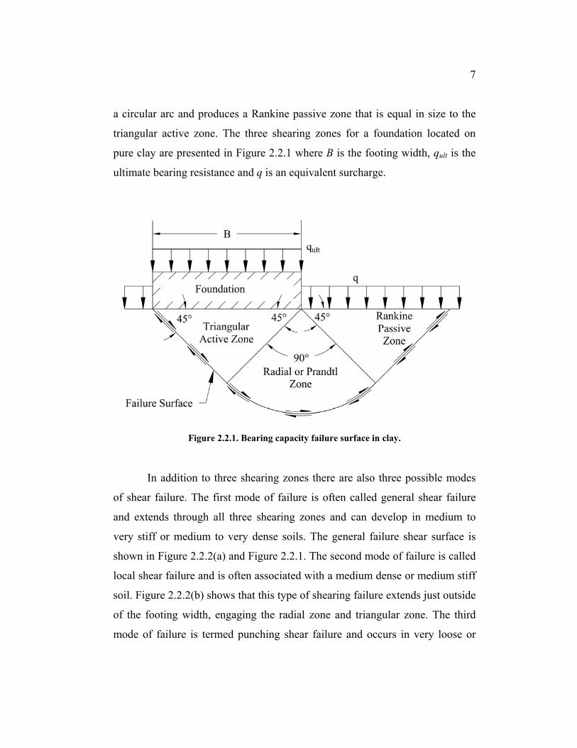
a circular arc and produces a Rankine passive zone that is equal in size to the

triangular active zone. The three shearing zones for a foundation located on

pure clay are presented in Figure 2.2.1 where B is the footing width, qult is the

ultimate bearing resistance and q is an equivalent surcharge.

Figure 2.2.1. Bearing capacity failure surface in clay.

In addition to three shearing zones there are also three possible modes

of shear failure. The first mode of failure is often called general shear failure

and extends through all three shearing zones and can develop in medium to

very stiff or medium to very dense soils. The general failure shear surface is

shown in Figure 2.2.2(a) and Figure 2.2.1. The second mode of failure is called

local shear failure and is often associated with a medium dense or medium stiff

soil. Figure 2.2.2(b) shows that this type of shearing failure extends just outside

of the footing width, engaging the radial zone and triangular zone. The third

mode of failure is termed punching shear failure and occurs in very loose or

8

soft soils in which shearing is limited to the zone of soil directly beneath the

footing as is depicted in Figure 2.2.2(c) (Das, 2011).

Figure 2.2.2. Bearing capacity failure mechanisms, modified after (Vesic, 1973).

General shear failure is the most common mode of failure and is often

the only mode checked in foundation design. Loading of undrained clays are

governed by general shear failure and proper settlement analyses inherently

protect against local and punching shear failures (Coduto, 2001). When

computing bearing capacity it is often assumed that the soil will behave in a

9

rigid-perfectly plastic manner which would produce sudden failure when the

shear strength of the soil is exceeded. Although this idealized analysis ignores

the manner in which capacity develops with displacements, it has historically

provided a good estimate of the ultimate limit state.

Terzaghi (1943) proposed several modifications to approximate bearing

capacity based on a two-dimensional plane strain analysis of a continuous

foundation. The original continuous foundation approximation was developed

assuming a shear failure surface similar to that presented in Figure 2.2.1 where

the shear strength of the soil was defined by the Mohr-Coulomb failure

criterion presented in Equation (2.1):

where is the shear strength of the soil, ′ is the effective cohesion of the soil,

′ is the effective stress at the location of interest, and ′ is the effective

friction angle of the soil.

Terzaghi (1943) modified the two-dimensional analysis to account for

three-dimensional effects of square and circular foundations using empirical

coefficients achieved through model tests. The resulting approximations for

rigid footings are provided in Table 2.2.1 and comprise three capacity

components: (1) capacity due to cohesive soil strength, (2) capacity due to

surcharge strength, and (3) capacity provided by frictional passive soil

pressures. Each capacity component is modified by bearing capacity factors,

which account for geometric variations in the failure surface and are expressed

as a function of the effective friction angle. Foundations that are rapidly loaded

and located on saturated clay are often designed using total stress (ϕ’ = zero)

analyses due to the lack of pore water dissipation and difficulty associated with

predicting pore water pressure generation in the field. When a load is applied to

′ ′ (2.1)

10

a foundation at a rate faster than the soil drainage, the total stress increase in the

soil is equal to the increase in pore water pressure which and depending on the

soil behavior, will alter the available shear strength of the soil.

Table 2.2.1. Terzaghi bearing capacity approximations.

Footing Type Approximation1,2 Eqn.

Continuous 12

(2.2)

Square 1.3 0.4 (2.3)

Circular 1.3 0.3 (2.4)

γ = Unit weight of the soil

Nc, Nq, Nγ = Unitless Terzaghi bearing capacity factors

Subsequent investigators (Hansen, 1970; Vesic, 1973) have developed

additional capacity factors to incorporate variations in foundation shape and

depth which are given by:

where ′ , ′ , ′ are unitless bearing capacity factors, , , are

footing shape correction factors, and , , are footing depth correction

factors. In undrained loading conditions the frictional passive strength provides

12

′ (2.5)

11

no additional foundation capacity. The resulting reduced bearing capacity

equation is given by:

Several different methods exist in the literature to calculate bearing

capacity factors. The research presented in this document utilizes Vesic bearing

capacity (Vesic, 1973), DeBeer shape (De Beer, 1970), and Hansen depth

factors (Hansen, 1970) as shown in Table 2.2.2 and Table 2.2.3. In undrained

capacity analyses where ϕ’ is assumed equal to zero, Equations (2.7) and (2.8)

reduce to 5.14 and 1.0, respectively (Vesic, 1973).

Table 2.2.2. Bearing capacity factors.

Factor Type Factor Formulation Eqn.

Vesic Bearing Capacity

45°′2

(2.7)

′ 1 cot (2.8)

Equation (2.9), presented in Table 2.2.3, represents the increase in

capacity from three-dimensional effects of a square foundation. An increase in

capacity will develop due to an increase in the size of the failure surface when

3-D effects are taken into account; it is important to note that no increase in

capacity will develop from 3-D surcharge effects as is presented in Equation

(2.6)

12

(2.10). The effect of embedment on capacity linearly increases with depth when

Df is shallower than B, until Df exceeds B after which embedment effects

increase hyperbolically to a limiting value. The capacity provided from

surcharge is not modified with increasing embedment depth, as shown in

Equations (2.12) and (2.14).

Table 2.2.3. Depth and shape factors.

Factor Type Factor Formulation Eqn.

Brinch Hansen Shape Factors

1 0.2 (2.9)

1 (2.10)

Brinch Hansen Depth Factors

For 1 1 0.4 (2.11)

1 (2.12)

For 1 1 0.4 tan (2.13)

1 (2.14)

1Note: this quantity in radians. 2L = Length of footing

The bearing capacity analysis presented in Equation (2.6) neglects two

important considerations: the weight of the footing and an applied factor of

safety, FS. The net ultimate bearing resistance, qnet(u), accounts for the weight

of the footing and is given by:

13

(2.15)

where γf is the unit weight of the footing. In practice, displacements need to be

limited; to limit displacements and ensure that failure does not occur an

allowable bearing capacity is typically specified. Equation (2.16) presents the

net allowable bearing pressure:

2.2.2. Evaluation of Bearing Capacity from Load Test Data

Plate or footing load tests are sometimes performed to determine the

bearing capacity of a footing. A footing is loaded at a rapid rate and

displacement, δ, measurements are taken at load increments to develop a load-

displacement curve (Q-δ) or a bearing pressure-displacement (q-δ) curve.

Typical q-δ curves are presented in Figure 2.2.3.

The nonlinearity of q-δ curves makes it difficult to determine the

ultimate bearing pressure, qult. Based on observations of bearing pressure-

displacement behavior, Vesic (1973) suggested that the ultimate bearing

pressure may be obtained at a predefined displacement that ranges between 3

and 7 percent of the footing width up to a maximum value of ten percent in

cases where a maximum value cannot be established with confidence. More

recently, Decourt (1992) suggested 0.75% of the diameter of the footing.

De Beer (1970) proposed a method in which the normalized

displacement (δ/B) versus normalized pressure (q/qult) is plotted on a log-log

scale; this method of plotting produces two approximately linear portions of a

(2.16)

14

q-δ curve. The point of intersection is considered to be the ultimate bearing

pressure. The method proposed by De Beer can produce results that are

dependent on the designer and often produces a range of ultimate values

(Paikowsky & Tolosko, 1999).

Figure 2.2.3. Typical bearing pressure-displacement curves after (Brand, et al., 1972)

Chin (1971) developed a method that assumes the q-δ curve is

hyperbolic. The Chin transformation consists of a plot of the ratio of the square

root of displacement to the applied load, Q, or bearing pressure, q, versus

displacement (Figure 2.2.4). For comparison, the corresponding q-δ curve is

plotted next to the Chin transformation. The initial portion of the Chin curve is

0

5

10

15

20

25

30

35

40

0 50 100 150 200 250

Dis

pla

cem

ent

(mm

)

Bearing Pressure (kPa)

BB1 (1.05 m)

BB2 (0.9 m)

BB3 (0.75 m)

BB4 (0.675 m )

BB5 (0.6 m)

15

commonly ignored due to partial mobilization of soil strength. As load is

applied to the foundation and transferred into the soil, the assumed shear failure

surface begins to develop and transform stresses into strains. At initial strains

the failure surface is only partially mobilized and does not represent the

available capacity of the soil beneath the foundation. When the soil along the

shear failure surface becomes fully mobilized, an approximately linear

relationship develops in the Chin transformation and the ultimate bearing

resistance is reached. A linear regression may be performed to determine a best

fit linear trend; the slope of the linear portion, C1, is inversely proportional to

the ultimate bearing resistance:

1 (2.17)

Hirany and Kulhawy (1988) and Paikowsky and Tolosko (1999)

provide an overview of several other methods, such as Davisson’s Offset

Criterion for driven piles and Brinch Hansen’s method, which are not discussed

herein because they can be subjective and are used for pile load tests. A

preferred ultimate load criterion is independent of experience and is based

solely on a mathematical procedure that will yield consistent results.

Often, due to limitations in reaction capacity and safety, footings are not

loaded to failure, thus it is pertinent to estimate the remaining portion of the q-δ

curve to extrapolate an ultimate bearing resistance. Jeon and Kulhawy (2001)

suggested a hyperbolic relationship to extrapolate the unknown portion of the

q-δ curve with reasonable results. Although extrapolation may produce

reasonable approximations for ultimate bearing pressures, uncertainty that

develops from extrapolation could produce unrealistic q-δ curves and caution

16

must be exercised when producing extrapolated q-δ curves to estimate

displacements.

Figure 2.2.4. Example of Chin load-displacement transformation with data from Figure

2.2.3.

2.3. Settlement

The previous section discussed methods to analyze bearing capacity of

foundations. The second limit state design that geotechnical engineers must

design for is excessive total or differential settlement which may cause lack of

functionality for the supported structure or potentially lead to bearing failure.

0.00

0.05

0.10

0.15

0.20

0.25

0.30

0.35

0.40

0.45

0.50

0

20

40

60

80

100

120

140

160

180

200

0 10 20 30 40

Sq

uare R

oot of δ/q (m

m/k

Pa) 0.5

Bea

rin

g P

ress

ure

(k

Pa)

Displacement (mm)

BB1 (1.05 m)

Initial Chin Transform.

Linear Chin Transform.

17

2.3.1. Total Settlement

The total settlement, St, which can develop beneath a footing, comprises

three components: immediate (or distortion), primary (consolidation), and

secondary (creep) settlement, and is given by:

(2.18)

where is the immediate settlement, is the primary settlement, is the

secondary settlement. In this work the term distortion settlement is used

interchangeably with distortion displacement.

Immediate settlement, often called distortion displacement, is the focus

of this research and is the result of rapid loading. Temporally, primary

settlement occurs after immediate settlement and is the product of water

pressure dissipation from soil pores and simultaneous transfer of the applied

load to the soil skeleton. This type of settlement usually develops over an

extended time period that can range anywhere from several hours to tens of

years for coarse-grained granular soils to fine-grained cohesive soils,

respectively. Some researchers suggest that secondary settlement occurs during

primary settlement in granular soils (Mitchell & Soga, 2005). Secondary

settlement develops after primary consolidation is complete and results from

soil particle reorientation and soil structure deterioration in highly plastic and

organic soils. Each settlement component develops from different mechanisms

and affects each soil type differently. Table 2.3.1 shows the potential for each

settlement component based on soil type.

18

Distortion settlement has the potential to occur in all soil types, whereas

primary and secondary compression settlements vary with soil type. This

research will focus on the distortion settlement of cohesive soils.

Table 2.3.1. Potential for settlement component, adapted from (Holtz, 1991).

Soil Type Si Sc Ss

Sands Yes No No

Clays Possibly Yes Possibly

Organic Soils Possibly Possibly Yes

2.3.2. Distortion Settlement

There are two primary factors that affect the mode of settlement:

hydraulic conductivity, and compressibility. In clean granular soils, primary

settlement develops almost immediately due to its relatively large hydraulic

conductivity. Contrastingly, in a clay layer, primary settlement may take years

to complete. However, in cases where loading is rapid, pore water pressures are

not able to dissipate; therefore the soil structure must resist the applied loads.

This leads to a specific design technique called a total stress approach. This

approach uses undrained soil shear strengths, su, which can be approximated

using field or laboratory tests (Holtz, et al., 2011).

In granular soils, typical construction loading does not occur rapidly

enough to initiate undrained conditions and distortion settlement is the result of

compression, distortion, and reorientation of the soil particles (Foye, et al.,

2008). In general construction, distortion displacement in sands comprises the

19

majority of settlement. In clays, the principal contributor to total settlement is

typically primary settlement, but varies with loading rate, duration of loading,

and stress history. However, there are many cases in which the immediate

settlement has proven to be significant in clays. Two specific cases are when

the mobilized shear stresses exceed approximately 50 percent of the available

shear strength, and in highly plastic clays or organic soils. It has been noted that

the magnitude of immediate settlement can be indicative of the magnitude of

other settlement mechanisms (Foott & Ladd, 1981). Foott & Ladd (1981)

measured an increase in creep settlement in soils that had a significant amount

of immediate settlement.

Additionally, it has been noted that distortion displacement is related to

bearing capacity. As a load is applied to a foundation on saturated clay such

that the soil behaves undrained, displacement will develop to mobilize the shear

strength of the soil. If the applied load is greater than the available shear

strength of the soil, excessive displacement will develop in the form of bearing

failure. Therefore, a model that accurately predicts distortion displacement as a

function of load could also be used to approximate bearing capacity.

2.4. Selected Aspects of Cohesive Soil Behavior

Cohesive soils exhibit stress-strain-strength behavior that depends on

many factors such as stress history, hydraulic conductivity, compressibility, and

strain rate. This section discusses the effect of stress history and strain rate on

general clay behavior and its influence on this research.

20

2.4.1. Stress history

Soil is a non-conservative material, which means it has a “memory” of

previous stresses. When a soil is loaded and unloaded, the soil structure is

altered and will influence the soil’s behavior if it is later reloaded (Holtz, et al.,

2011). The strength and stiffness of clay is largely dependent upon the initial

vertical effective stress, σ’vo, and the preconsolidation pressure, σ’p. The

preconsolidation pressure is defined as the maximum previously applied stress,

and it is found by conducting consolidation tests on specimens. The

overconsolidation ratio, OCR, is a measure of the magnitude of previous

maximum effective stress in relation to the existing effective stress condition

and is given by:

The determination of the preconsolidation pressure is dependent upon

the quality of the soil specimen and consolidation curve that results from a

consolidation test. Foott and Ladd (1974) noted that highly disturbed samples

produced curves that made it difficult to accurately determine the

preconsolidation pressure and recommended the use of a testing procedure

known as Stress History and Normalized Soil Engineering Properties

(SHANSEP), which evaluates the stress history of the soil by comparing the

initial vertical effective stress and different maximum past pressures, σ’vm, to

determine OCR variation throughout the deposit. Plotting the variation in OCR

against the ratio of undrained shear strength to initial vertical effective stress

produces SHANSEP curves that can be used to produce an undrained shear

strength profile (Stuedlein, 2008). The SHANSEP procedural methodology

′′

(2.19)

21

detailed in Foott and Ladd (1974) normalizes soil strength properties and

accounts for variations that develop due to sample disturbance.

2.4.2. Strain Rate

An investigation conducted by Richardson and Whitman (1963) into the

effect of strain rate on the behavior of clay showed that the undrained shear

strength varies with quantity of strain. At axial strains greater than five percent,

an increase in strain rate produces an increase in resistance to compression and

a reduction in pore water pressure buildup, while the effective stress ratio

remains unaffected or exhibits a slight decrease. At small axial strains (i.e. less

than 0.5 percent) an increase in strain rate produces an increase in the effective

stress ratio, σ1/σ3, and the principal stress difference, (σ1-σ3). Richardson and

Whitman (1963) interpreted these results to imply that the strain rate effect at

large strains is related to volume change whereas the increase in strength at

small strains results from distortion of the soil particles. Thus clay soil behavior

is fundamentally different at different strain levels.

Sheahan et al. (1996) investigated the effects of strain rate and stress

history on the undrained shear behavior of saturated clay. Twenty five

specimens of re-sedimented Boston blue clay were subjected to CKoUC triaxial

tests at different strain rates and OCRs using the SHANSEP reconsolidation

procedure. Specimens were consolidated to four OCRs (one, two, four and

eight) and tested at four constant axial strain rates, εa, 0.05, 0.5, 5 and 50

percent/hr. The results of this experimental program indicate that strain rate and

stress history have a large effect on the undrained shear strength of saturated

clay.

The reference strain rate, 0.5 percent/hr., was chosen because a range of

0.5 to 1 percent/hr. is typically recommended in practice. The reference stress-

22

strain curves were than normalized by the maximum vertical effective stress,

σ’vm, to develop normalized stress-strain curves. Typically, the maximum

vertical effective stress is equivalent to the consolidation pressure, σvc,

however, Sheahan performed two tests that were subjected to pre-shear

unloading, and the maximum vertical effective stress was not equivalent to the

consolidation pressure for those two samples.

Sheahan et al. (1996) conducted additional tests at varying strain rates

and OCRs to assess the effect of stress history and strain rate on saturated clay

behavior. The experimental results presented by Sheahan et al. (1996) indicate

that as the strain rate increases the normalized undrained shear strength also

increases. Saturated clays that are subjected to strain rates that are greater than

about ten percent per hour are rate sensitive, regardless of stress history.

Sheahan et al. (1996) also noted that as OCR increases, the effect of strain rate

on undrained shear strength reduces and as the strain rate increases the

undrained shear strength increases proportionally. Additionally, shear strength

of specimens with large OCRs tested at low strain rates may be independent of

strain rate. Sheahan et al. (1996) suggested that a threshold strain rate may exist

and is defined as the strain rate below which the strain rate has little to no effect

on the soil behavior. This could prove to be of importance at low OCRs. The

effect of strain rate on the normalized undrained shear strength or the rate

sensitivity, ρ0.5, is presented in Figure 2.4.1.

The primary mechanism for an increase in strength as strain rate

increases is the development of shear-induced negative pore pressures. In soils

with OCRs less than two, undrained shear strength increases because of the

suppression of induced excess pore pressures and the resulting effect on the

effective stress friction angle. At OCRs approximately greater than two,

23

strength increases because of the formation of negative shear-induced pore

pressures (Sheahan, et al., 1996).

Sheahan et al. (1996) also suggested, based on normalized soil shear

behavior, that the strain at which the peak undrained shear strength occurs is

independent of strain rate and varies for a given OCR. The assumption of peak

strain independency provides a basis for modeling rate dependent stress-strain

behavior using the undrained shear strength and the strain at failure, εf.

Figure 2.4.1 Normalized undrained shear strength vs. strain rate for re-sedimented

Boston Blue Clay after (Sheahan, et al., 1996).

24

2.5. Application of Elasticity Theory to Displacements of Shallow

Foundations

As a load is applied to a foundation the mechanism that transfers load to

stresses in the soil is a function of several factors, such as the rigidity of the

foundation, soil stiffness, soil strength, and the magnitude of strain. In saturated

cohesive soils, elasticity theory is widely accepted as the standard of practice to

approximate stresses that develop in the soil as a function of loading boundary

conditions. In homogeneous soil masses measured stress distributions agree

reasonably well with those calculated using elasticity theory, which is likely

because the assumption of small deformations is valid (Holtz, 1991). When

elasticity theory is used in layered systems or in large strain applications it is

notably inaccurate due to the assumption of no inter-layer shear stress and

nonlinear soil behavior.

2.5.1. Elastic Stress Distributions

Stresses attenuate with radial distance away from the loading boundary.

Boussinesq developed a solution for a perpendicular point load on a linear

elastic half space that is solely dependent on depth. Most foundations cannot be

treated as point loads; however, stress distributions within an elastic half space

due to a loaded area may be determined by integrating Boussinesq’s solutions.

Stress distributions are dependent upon the stiffness of the foundation and

resulting boundary conditions. A uniformly loaded flexible circular foundation

loaded on an elastic half space will produce approximately 1.27 (4/π) times the

amount of settlement at the center of the foundation than that of a rigid

foundation (Mayne & Poulos, 1999). The variation in magnitude of settlement

25

is chiefly due to the change in stress distribution resulting from the bending of

the foundation. The research presented herein will focus on rigid foundations.

Much of the proposed work for settlement calculations were developed

for circular footings. The equivalent circular footing diameter, Beq, may be used

to model square and rectangle foundations by:

4 (2.20)

The rigidity of a foundation is difficult to determine because the

foundation’s flexibility depends on the underlying soil. Borowicka (1936)

proposed that the stiffness of a foundation can be assessed using the soil

modulus and geometric properties of the foundation:

16

11

2 (2.21)

where is the foundation stiffness, is Poisson’s ratio of the soil, is

Poisson’s ratio of the foundation, is Young’s modulus of the foundation,

is Young’s modulus of the soil, and is the foundation thickness.

Brown (1969) proposed an alternate method for approximating the

stiffness of a foundation:

2 (2.22)

26

Mayne & Poulos (1999) differentiated rigid and flexible foundations by

their stiffness characteristics, given by:

Perfectly Rigid Kf > 10

Intermediate Flexibility 0.01 ≤ Kf ≤ 10

Perfectly Flexible 0.01 < Kf

For large stiffness values, the footing can be considered perfectly rigid,

whereas footings with low stiffness values can be considered perfectly flexible.

A perfectly flexible footing will generate uniform contact pressures on the soil

subgrade, whereas rigid footings will develop a uniform displacement profile.

The different contact pressures and displacement profiles that develop with

varying footing stiffness are shown in Figure 2.5.1.

Contact pressures and settlement profiles vary with soil types. It is

assumed that cohesive soils behave as a purely elastic medium, whereas

granular soils derive stiffness and strength from confinement. As a result,

contact pressures at the edge of rigid footing on an elastic medium greatly

exceed those of pressures in a granular soil mass. Contact pressures at the edge

of a rigid footing will increase with applied load until the ultimate shear

strength of the soil is reached. If an elastic medium with an assumed infinite

strength were to be heavily loaded with a large load, the resulting contact

pressures at the edge of the rigid footing would be infinite. In practical cases,

the shear strength, τf = su, of the soil limits the contact pressures.

27

Figure 2.5.1. Contact pressures for varying soil and footing rigidity type, from (Holtz,

1991).

Carrier & Christian (1978) compared elasticity theory-based stress

distributions to stress distributions developed using finite element analyses

(FEA). The comparison of stresses at Df/B between 0.3 and 3, H/B between 0.3

and 10 and L/B between 1 and 5 produced errors that were typically less than

10% and generally less than 20%.

2.5.2. Elasticity-based Distortion Settlement

The previous section discussed stress distributions that develop within

soil due to an applied load. In elastic material the quantity of displacement is

proportional to the applied load or stress. In bearing capacity analyses a linear

elastic-perfectly plastic model is often used to estimate distortion displacement

that will occur prior to bearing failure. Linear elastic-perfectly plastic soil

28

constitutive behavior is characterized as having a perfectly linear elastic portion

until an ultimate resistance is reached, at which point strain develops with no

further increase in stress, as presented in Figure 2.5.2.

Figure 2.5.2. Linear elastic-perfectly plastic soil behavior.

The assumption of linear elastic-perfectly plastic soil behavior greatly

simplifies the computational effort required to predict distortion displacement.

Carrier and Christian (1978) found that the stress distributions developed from

FEA, presented in Figure 2.5.3, used in conjunction with embedment factors

proposed by Burland (1970), presented in Figure 2.5.4, produce the most

reasonable values of displacement and recommended the following average

settlement calculation:

(2.23)

29

where is Burland’s embedment correction, is Carrier and Christian stress

distribution correction. The formulation is generic and assumes the undrained

Poisson’s ratio is 0.5 for clay.

Figure 2.5.3. Stress distributions in an elastic layer, after (Carrier & Christian, 1978).

Building upon earlier work, Mayne and Poulos (1999) developed a

distortion settlement formula for circular foundations that accounts for

variations in Poisson’s ratio, soil modulus variation, foundation rigidity, and

embedment effects is given by

1 (2.24)

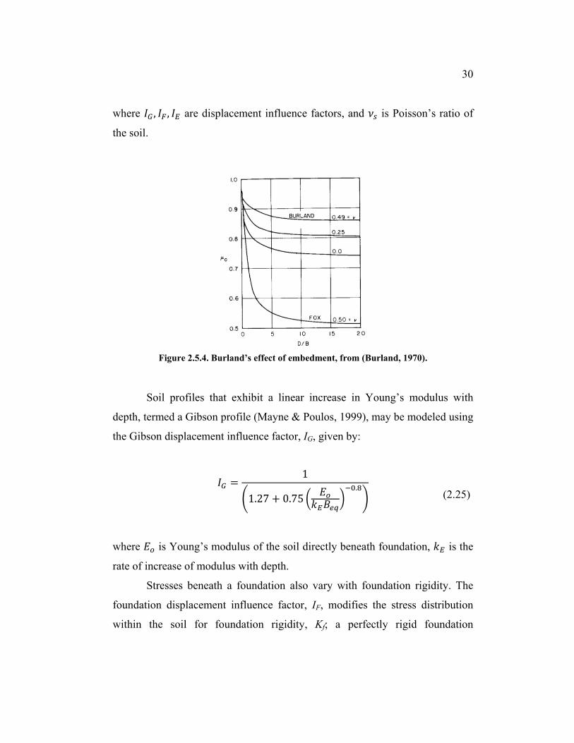
30

where , , are displacement influence factors, and is Poisson’s ratio of

the soil.

Figure 2.5.4. Burland’s effect of embedment, from (Burland, 1970).

Soil profiles that exhibit a linear increase in Young’s modulus with

depth, termed a Gibson profile (Mayne & Poulos, 1999), may be modeled using

the Gibson displacement influence factor, IG, given by:

1

1.27 0.75.

(2.25)

where is Young’s modulus of the soil directly beneath foundation, is the

rate of increase of modulus with depth.

Stresses beneath a foundation also vary with foundation rigidity. The

foundation displacement influence factor, IF, modifies the stress distribution

within the soil for foundation rigidity, Kf; a perfectly rigid foundation

31

approaches π/4, while a perfectly flexible foundation approaches unity (Mayne

& Poulos, 1999). The displacement influence factor is given by:

4

14.6 10

(2.26)

The embedment influence factor, IE, is Burland’s embedment influence

factor previously labeled as μo in Equation (2.23) and presented in Figure 2.5.4.

Regression analyses on Burland’s embedment influence factor performed by

Stuedlein (2010) yielded:

11

3.5 . . 1.6

(2.27)

2.5.3. Finite Element Analysis-based Approach

D’appolonia (1971) performed finite element analyses using a linear

elastic-perfectly plastic soil constitutive model to estimate the settlement ratio,

SR, defined as the ratio of elastic settlement computed without considering local

yield, ρe, to the actual settlement that occurs based on the applied stress ratio,

q/qult. Figure 2.5.5 provides charts for strip foundations to approximate q-δ

curves based on layer thickness, foundation width, and initial shear stress ratio,

f. The initial shear stress ratio relates the applied stresses to the available

strength in the soil and is given by:

′ ′2

12

(2.28)

32

where is the initial shear stress ratio, ′ is the initial vertical effective

stress, ′ is the initial horizontal effective stress, is the Undrained shear

strength of the soil, and is the lateral earth pressure coefficient.

The settlement ratio is combined with conventional elasticity theory

approximations to estimate immediate settlement, as given by:

where is the immediate settlement, is the displacement based on

conventional elastic theory, and is the settlement ratio.

D’Appolonia et al. (1971) noted that the curves presented in Figure

2.5.5 were limited to a homogeneous soil profile exhibiting isotropic undrained

shear strength and loaded with a strip footing. They compared the effect of

strength anisotropy and strength variation on settlement behavior, and found

that strength anisotropy does not have an important effect on immediate

displacement. D’Appolonia et al. (1971) discussed two types of strength

variation: non-homogeneity with respect to modulus and with respect to the

undrained shear strength. Effects of variation in the undrained modulus on q-δ

curves are limited to the stress distribution produced from Boussinesq theory

and are directly proportional to the undrained modulus, Eu. Therefore, Figure

2.5.5 is approximately valid if spatial variations in Eu are accounted for during

computation of elastic displacement, e.

Variation in the initial shear stress ratio and undrained shear strength

affects the shape of settlement curves more than that of undrained modulus.

D’Appolonia et al. (1971) noted that Figure 2.5.5 may be used when the initial

shear stress ratio is averaged over a depth equal to the foundation width.

(2.29)

33

D’Appolonia et al. (1971) also noted very little difference in settlements

between rigid or flexible and strip or circular footings especially if the soil

profile is not highly stratified. Application of Figure 2.5.5 may provide

reasonable approximates of q-δ curves.

Figure 2.5.5. Settlement ratio with applied stress ratio, from (D'Appolonia, et al., 1971).

34

Stuedlein et al. (2010) compared observed q-δ curves to those predicted

using the method proposed by D’Appolonia et al. (1971) and an estimated

elastic modulus (Holtz, 1991). The comparison in Figure 2.5.6 indicates that

the predicted q-δ curves are relatively stiffer than the observed curves and at

larger strains greatly under-predicts the amount of immediate displacement.

This is likely due to the assumption of linear elastic-perfectly plastic soil

behavior used in the FEA to develop Figure 2.5.5.

Figure 2.5.6. Observed full scale footing displacements compared to displacements

predicted after the method of D’Appolonia et al. (1971): (a) large 2.74 m square footing;

(b) small 0.76 m circular footing, from (Stuedlein & Holtz, 2010).

2.5.4. Use and Limitations of Young’s Modulus in Displacement Estimation

The selection and use of a single elastic modulus inherently produces

errors in the predicted stress-strain behavior (Figure 2.5.7). Slight variations in

an elastic modulus could lead to large variations in a predicted q-δ curve,

particularly at larger strains when the ultimate shear strength of the soil has

been exceeded.

35

It is important to note that methods presented in the literature use a

single elastic modulus for soil behavior. Although this can greatly reduce the

computational effort to estimate distortion settlement, it has been shown that

these methods can produce highly variable results (Roberts & Misra, 2010).

The use of a simplified linear elastic-plastic soil constitutive model to predict

nonlinear soil behavior provides intrinsic model errors, and when combined

with inherent soil variability, can produce unreasonable results (Holtz, 1991).

The intrinsic errors propagate throughout the soil profile as the nonlinearity

increases, particularly in overconsolidated soils.

Figure 2.5.7. Linear elastic vs. nonlinear stress strain behavior.

Depending on the design scenario, a designer can select from three

types of Young’s moduli: the initial modulus, Ein, the secant modulus, Esec, and

the tangent modulus, Etan (Figure 2.5.8). The tangent modulus is defined as the

slope at any portion of the stress-strain curve and the secant modulus is defined

as the slope of a line from the origin to any point on the stress-strain curve.

36

Young’s modulus is often characterized by its loading condition and the

primary focus of this research is on the initial undrained Young’s modulus.

The initial undrained Young’s modulus, Eu, is correlated to su (Kulhawy

& Mayne, 1990). Duncan and Buchignani (1987) suggested a relationship using

a K-factor that is based on OCR and PI. The relationship modifies the

undrained shear strength to estimate Eu and K is read from Figure 2.5.9. The

relationship is given by:

Figure 2.5.8. Various types of elastic modulus.

(2.30)

37

Figure 2.5.9. Variation in K-factor based on OCR and PI, from (Duncan & Buchignani,

1987).

2.6. Nonlinear Distortion Displacement Models

Recently, several authors (Osman & Bolton, 2004; Foye, et al., 2008;

Elhakim & Mayne, 2006) have pointed to the limitations of linear elastic-

perfectly plastic model behavior and developed nonlinear distortion

displacement models that attempt to more accurately estimate displacements.

These models typically rely on finite element solutions to produce q-δ curves

and are discussed below.

38

2.6.1. Mobilisable Strength Design (MSD)

Osman & Bolton (2004) presented a method for determining immediate

displacements that uses a defined displacement field with a plastic deformation

mechanism to estimate footing displacements. The defined displacement field

underneath a footing is similar to Figure 2.2.1. The average mobilized shear

strain, γmob, that develops within the mobilized displacement field is derived

from a spatial average of the engineering shear strain, γe, over the entire volume

of the displaced zone. The resulting formulation for the average shear strain

was found to be equal to:

(2.31)

where Mc is 1.33 for square footings and 1.35 for circular footings.

A q-δ relationship was developed through the use of conversion factors

to transform a stress strain curve into a q-δ curve. The stress axis is transformed

into a load axis by multiplying by a bearing capacity coefficient, N’c, and the

strain axis is converted to displacement by dividing it by the displacement

coefficient, Mc. The displacement coefficient was derived analytically using an

upper-bound plasticity solution. The transformation process is presented in

Figure 2.6.1 where Ncv and Mcv are the bearing capacity and displacement

coefficients for a vertical loading case (Osman, et al., 2007).

Although the method proposed by Osman et al. (2007) may be simple

and produce reasonable results, it requires that a triaxial test be conducted on a

high quality specimen taken from a specific depth to produce valid results.

39

Sampling disturbances combined with soil variability will greatly affect the

predicted q-δ response and can yield inaccurate results.

Figure 2.6.1. Illustration of the MSD approach, after (Osman, et al., 2007).

2.6.2. Small Strain Stiffness

Elhakim & Mayne (2006) presented a method that uses small strain

stiffness to predict intermediate and large strain soil characteristics. Small

strain stiffness can be an indicator of overall stiffness, as soils can exhibit linear

elastic behavior at very small strains. Small strain stiffness is only valid when

the strain in the soil has not exceeded the linear threshold strain, γtl, or the strain

at which modulus reduction occurs. The linear threshold strain varies with soil

type, tends to increase with PI, and can range between 0.01 and 0.0001%

(Vucetic, 1994).

In-situ and laboratory tests, such as seismic cone and resonant column

tests, can measure the constitutive soil behavior below the linear threshold

strain. The shear strain at failure, γf, is required to define the point at which an

40

increase in strain will not provide an increase in stress. Elhakim & Mayne

(2006) presented a correlation between the, PI, and failure shear strain for

cohesive soils:

Elhakim and Mayne (2006) adopted a single parameter logarithmic

modulus reduction scheme presented by Puzrin and Burlin (1996) to

extrapolate large strain soil behavior from small strain stiffness parameters. The

adopted model is computationally intensive and may not be applicable to load

tests in which large strains are evident.

As discussed earlier Richardson and Whitman (1963) noted that soil

behavior at small strains is dependent on particle distortion while soil behavior

at large strains is dependent on volumetric distortion. The method proposed by

Elhakim & Mayne (2006) is computationally intensive and assumes that soil

behavior at small strains is comparable to soil behavior at large strains, and this

assumption may not be valid. The comparison presented in Figure 2.6.2 uses

input parameters correlated from cone penetration test (CPT) data to predict q-δ

curves using the method proposed by Elhakim and Mayne (2006) and indicates

that the proposed method produces a much stiffer curve than the observed q-δ

curves.

0.23 (2.32)

41

Figure 2.6.2. Comparison of predicted Elhakim and Mayne q-δ vs. Observed, data from

Stuedlein et al. (2010).

2.6.3. Nonlinear Elastic Perfectly Plastic Soil Behavior Models

Foye et al. (2008) used FEA to develop charts that may be used to

approximate the displacement of a footing. The use of a hyperbolic soil

constitutive model originally developed by Kondner (1963) and later modified

by Viggiani and Atkinson (1995) was employed by Foye et al. (2008). The

modified hyperbolic soil constitutive model is given by:

′ (2.33)

0

100

200

300

400

500

600

700

800

0 50 100 150 200 250

Ap

pli

ed B

eari

ng

Pre

ssu

re (

kP

a)

Displacement (mm)

Predicted Large FootingPredicted Small FootingLarge FootingSmall Footing

42

where is a reference stress typically equal to 1 kPa), ′ is the mean

effective stress, is the initial shear modulus, and , , are unitless PI

based parameters.

The reference strain, pr, is commonly taken as 1 kPa to produce a

unitless stress component. Viggiani and Atkinson (1995) used small-strain

measurements from bender element tests to develop correlations for A, n and m

parameters which depend on the PI of the soil and the current strain. The

Viggiani and Atkinson (1995) correlations are:

3,790.0 . (2.34)

0.109 0.4374 5 (2.35)

0.015 0.1863 5 (2.36)

The charts developed by Foye et al. (2008) are presented in Figure

2.6.3, where qb,net is the difference between the load acting over the footing and

the vertical effective stress in the surrounding soil and H is the depth to a rigid

boundary. The formulation to calculate displacement is:

, (2.37)

where Iq is Foye’s influence factor.

Foye et al. (2008) performed a sensitivity analysis to assess the effects

that varying soil parameters in the FEA have on the influence factor by

comparing soil parameters directly at the base of the footing (Figure 2.6.4a) and

averaging the soil parameters over depths of 2B and B below the footing

(Figure 2.6.4b). This comparison indicates that average soil parameters produce

43

more consistent values of influence factors and variations in soil parameters

will produce conservative estimates of displacement.

Figure 2.6.3. Influence factors for distortion settlement, after (Foye, et al., 2008); (a) strip

footings; (b) square footings; and (c) rectangular (L/B=2) footings

Figure 2.6.4. (a) Iq computed from soil parameters at the base of a typical footing and (b)

Iq computed from average soil parameters (Foye, et al., 2008).

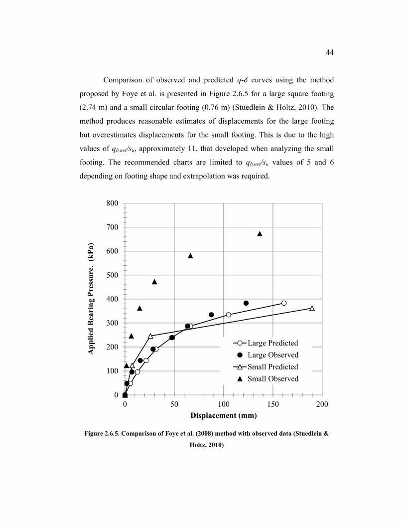
44

Comparison of observed and predicted q-δ curves using the method

proposed by Foye et al. is presented in Figure 2.6.5 for a large square footing

(2.74 m) and a small circular footing (0.76 m) (Stuedlein & Holtz, 2010). The

method produces reasonable estimates of displacements for the large footing

but overestimates displacements for the small footing. This is due to the high

values of qb,net/su, approximately 11, that developed when analyzing the small

footing. The recommended charts are limited to qb,net/su values of 5 and 6

depending on footing shape and extrapolation was required.

Figure 2.6.5. Comparison of Foye et al. (2008) method with observed data (Stuedlein &

Holtz, 2010)

0

100

200

300

400

500

600

700

800

0 50 100 150 200

Ap

pli

ed B

eari

ng

Pre

ssu

re,

(kP

a)

Displacement (mm)

Large Predicted

Large Observed

Small Predicted

Small Observed

45

2.7. Summary of Literature Review

The current state of practice for predicting distortion displacement

assumes that linear elastic, perfectly plastic soil behavior is valid. Accordingly,

current methods do not accurately predict true, nonlinear soil behavior. Slight

variations in estimation of soil parameters may produce unrealistic

displacement estimates due to inherent errors in the predicted linear elastic soil

behavior. Other methods available in the literature are either computationally

intensive or rely on FEAs that assume homogeneous and isotropic soil

conditions and are limited to specific stress conditions. These advanced

methods may not be applicable to realistic scenarios and are limited to generic

soil profiles.

The literature review has discussed the following points that are

pertinent to this research:

1. Structural loads may cause significant distortion settlement in the

underlying soils, which may lead to unacceptable building

performance;

2. The magnitude of distortion displacement may indicate the proximity

of a foundation to bearing capacity failure;

3. Increasing the rate of loading increases the undrained strength of

saturated clays but does not alter the strain at failure;

4. Accepted methods of estimating distortion displacement rely on the

assumption of linear elastic, perfectly plastic soil behavior which can

produce unreasonable results; and

5. Proposed nonlinear methods do not adequately capture true q-δ

behavior and therefore may produce inaccurate estimates of distortion

settlement.

46

Chapter 3: Research Objectives and Program

3.1. Objectives of this Study

The purpose of this study is to quantify the accuracy and uncertainty in

the prediction of bearing capacity and immediate displacement of shallow

foundations on saturated clay. Specific objectives of this research include:

1. Evaluation of the accuracy of common bearing pressure-displacement

models;

2. Comparison of bearing capacity estimated using accepted methods

and capacity extrapolated from bearing pressure-displacement curves;

3. Assessment of the effect of variability in undrained shear strength and

model error associated with traditional approaches for computing

bearing capacity;

4. Comparison of undrained shear strength back-calculated from

calculated and extrapolated bearing capacities;

5. Comparison of actual bearing pressure-displacement curves with

those predicted using the Duncan-Chang model and elasticity theory;

and

6. Calibration of resistance factors for a bearing capacity model that

does not take into account the variability in undrained shear strength.

3.2. Research Program

The research program undertaken to achieve the objectives are

presented in Figure 3.2.1 and Figure 3.2.2, where all variables are defined in

the list of symbols and includes:

47

1. Develop database of footing load tests reported in the literature with

measured and/or estimated undrained shear strength and stiffness

(Chapter 4 and 5);

2. Estimate bearing capacity using accepted bearing capacity formulas

and compare to that determined from bearing pressure-displacement

curves (Chapter 6);

3. Back-calculate undrained shear strength using the Kondner hyperbolic

model and compare to measured and/or estimated values (Chapter 6);

4. Apply the Duncan-Chang hyperbolic model within a linear-elastic

stress field to predict strains and displacements beneath each footing

using stiffness correlation models (Chapter 7);

5. Back-calculate stiffness values using Duncan-Chang hyperbolic

model and compare with correlated values (Chapter 7);

6. Use stiffness values to calculate the bearing pressure required to

produce various amounts of displacement using accepted immediate

settlement estimation methods and compare to the actual

displacements (Chapter 7); and

7. Develop a bearing capacity model and calibrate resistance factors

(Chapter 8).

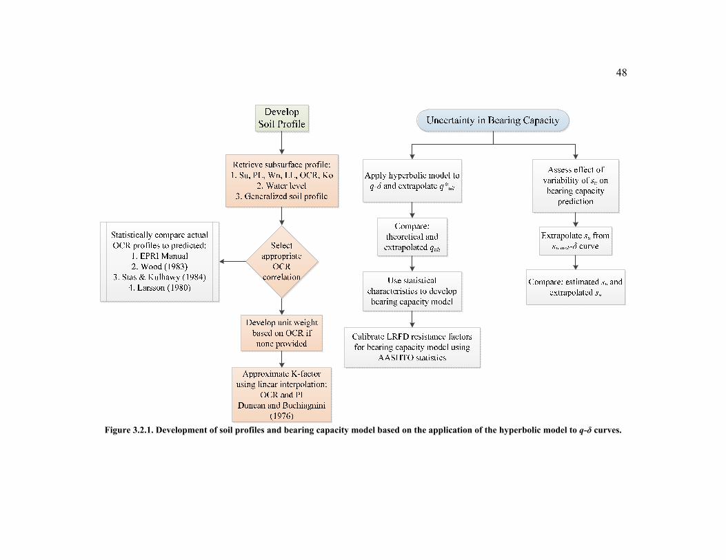
48

Figure 3.2.1. Development of soil profiles and bearing capacity model based on the application of the hyperbolic model to q-δ curves.

49

Figure 3.2.2. Flow chart of the research program for the assessment of the Duncan-Chang model.

50

Chapter 4: Database of Loading Test Case Histories

4.1. Introduction

The completion of the research program discussed in Chapter 3 requires

compiling data from previously performed footing load tests. Numerous case

histories exist in the literature that present bearing pressure-displacement curves

developed from footing load tests for shallow foundations on clay. The available

footing load tests were vetted for quality and compiled into a database. The

footing load test database is discussed and a brief overview of each case history is

presented.

4.2. Criteria and Selection of Case Histories

To evaluate the uncertainty in existing methods and provide the basis for

new models, a database of case histories was developed. The database was

initially populated with 24 case histories and was subsequently reduced to 12 case

histories based on the reporting and quality of particular soil parameters, as

outlined below:

1. Undrained shear strength, su;

2. Water contents and Atterberg limits;

3. Bearing pressure-displacement curves;

4. Loading rate;

5. Foundation size and rigidity.

Specifically, the selection criteria to assemble the database for the present

study include:

1. The soil profile must consist of cohesive soil and act in an undrained

manner;

51

2. The case history providing the load test data must have adequate

supporting test data (e.g., in-situ test information, laboratory test

information, etc.), particularly undrained shear strength;

3. The soil profile must be relatively uniform for the portion of the soil that

is being mobilized by the footing;

4. The load test data must provide information regarding the load test

setup, footing widths, embedment, material, etc.;

5. The footings must be rigid and have a depth of embedment less than 4B;

and,

6. The load test data must have been developed using a maintained load

test.

The data compiled in Table 4.3.1 presents the final 12 case histories vetted

per the criteria outlined above and provides a good start for a load-test database

that may be used for uncertainty quantification. The 12 rejected case histories are

summarized below:

Three case histories where the foundations were found to be flexible

(Schnaid, et al., 1993; Hoeg, et al., 1969; Nordlund & Deere, 1970);

Three case histories where there was a potential for drained loading

(Larsson, 1980; Consoli, et al., 1998; Pile, 1975);

One case history where the depth of embedment is greater than 4B

(Ward, et al., 1965), and

Five case histories that lacked pertinent soil information (Rilling &

Smoltczyk, 1994; Thamm, 1976; Bergfelt, 1956; Milovic, 1965; Han &

Ye, 1991).

52

4.3. Case History Index and Overview

A database index was developed to organize and compile the footings by a

few of the above categories. This is presented in Table 4.3.1, and is followed by

a brief discussion on each of the selected case histories. The quality of data

section of Table 4.3.1 is a subjective assessment of the case history based on the

provided information. It provides a general evaluation of the overall case history

in relation to the rest of the database and provides enough information to

minimize the amount of correlations required to develop required soil

parameters. For example, a “Good” case history would consist of subsurface

explorations well below the zone of loading influence, provide the loading rate,

foundation material, footing embedment, water level, and an OCR profile. A

lower quality case history is still usable but would lack one of these

characteristics and require additional correlations. The subsurface profiles for

each case history are presented in Appendix A, and the bearing pressure-

displacement behavior for each footing load test is presented in Appendix B.

4.3.1. Bangkok, Thailand - 1972

The Chao Praya Plain, located 40 km north of Bangkok, Thailand,

contains deep deposits of soft marine clay (Brand, et al., 1972). The generalized

soil profile consists of light to dark grey, soft clay with a PI of 48 and a liquidity

index (LI) of 0.73. The undrained shear strength was investigated using vane

shear strength tests (VST) and an approximate OCR of 10 was retrieved from

additional studies on the Chao Praya Plain (Moh, et al., 1969). Spread footings are

rare because of the strength and deformation characteristics of the soft clay.

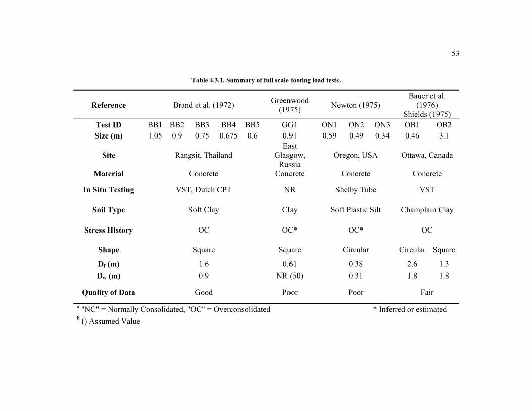
53

Table 4.3.1. Summary of full scale footing load tests.

Reference Brand et al. (1972) Greenwood

(1975) Newton (1975)

Bauer et al. (1976)

Shields (1975) Test ID BB1 BB2 BB3 BB4 BB5 GG1 ON1 ON2 ON3 OB1 OB2 Size (m) 1.05 0.9 0.75 0.675 0.6 0.91 0.59 0.49 0.34 0.46 3.1

Site Rangsit, Thailand East

Glasgow, Russia

Oregon, USA Ottawa, Canada

Material Concrete Concrete Concrete Concrete

In Situ Testing VST, Dutch CPT NR Shelby Tube VST

Soil Type Soft Clay Clay Soft Plastic Silt Champlain Clay

Stress History OC OC* OC* OC

Shape Square Square Circular Circular Square

Df (m) 1.6 0.61 0.38 2.6 1.3

Dw (m) 0.9 NR (50) 0.31 1.8 1.8

Quality of Data Good Poor Poor Fair

a "NC" = Normally Consolidated, "OC" = Overconsolidated * Inferred or estimated b () Assumed Value

54

Table 4.3.1. (continued): Summary of full scale footing load tests.

Reference Marsland & Powell (1980) Andersen and

Stenhamar (1982) Bergado et al. (1984)

Test ID CM1 HA1 HA2 RB1 Size (m) 0.865 1 0.3

Site Cowden, UK Haga, Norway Rangsit, Thailand

Material Steel Plates Steel Plates Concrete

In Situ Testing NR VST CPT

VST, CPT, SPT PMT

Soil Type Glacial Till Medium Stiff OC

Clay Bangkok Clay

Stress History OC* OC OC

Shape Circular Square Circular

Df (m) 3 0 0

Dw (m) 1 10 1

Quality of Data

Fair Good Fair


55


Reference Tand (1986) Hight et al. (1995 & 1997)

Jardine et al. (1993 & 1995)

Test ID TT1 TT2 TT3 TT4 TT5 TT6 TT7 TT8 BH1 Size (m) 0.58 0.58 0.58 0.58 0.58 0.58 0.58 0.58 2.2

Site Texas, USA Bothkennar, UK

Material Steel Plates Concrete

In Situ Testing PM, CPT, PP VST, CPT, SPT

PMT

Soil Type Stiff Sandy Clay Med. Stiff

Silty Clay to Clay

Slickensided Stiff to Very Stiff Clay

Soft Marine to Estuarine Clay

Stress History OC* OC* OC* OC

Shape Circular Square

Df (m) 1.5 0.78

Dw (m) 0.9 0.9 1.1 0.9

Quality of Data Fair Good


56


Reference Deshmukh (1994) Lehane (2003) Stuedlein & Holtz (2010)

Test ID BD1 BD2 BL1 TS1 TS2 TS3 Size (m) 0.6 0.6 2 0.76 0.76 2.74

Site Bombay, India Belfast, Ireland Texas, USA

Material Concrete Concrete Concrete

In Situ Testing SPT, PLT VST CPT

Seismic Wave CPT, SPT

Soil Type Soft Marine Clay Soft Clayey Silt Silty Fat Clay

Stress History OC* NC* OC

Shape Square Square Circular Square

Df (m) 0 1.6 0.61 0.61 0

Dw (m) 0.6 1.4 2.4

Quality of Data Fair Good Good


57

A majority of the foundation support for single and multiple story buildings

consist of grouped short wooden piles driven to depths of 5 to 8 m (Brand, et al.,

1972). Five square footing load tests, ranging in diameter from 0.6 to 1.05

meters, were conducted to provide a baseline to compare the effects short wooden

piles on bearing pressure-displacement curves. A native soil profile from the Chao

Praya plain is presented in Appendix A.

4.3.2. Glasgow, Scotland - 1975

This case history focuses on the effect of gravel piers as a method to

improve the bearing pressure-displacement behavior of clay soils (Greenwood,

1975). A footing load test was conducted at the test site as a baseline to measure

ground improvement methods. Stiff boulder clay underlies softer clays at depths

of about 3 m, for which the PI was approximately 30 with a LI of about 0.1. An

OCR of approximately 3.6 was correlated from a single reported undrained shear

strength value of 44 kPa. (Greenwood, 1975).

4.3.3. Corvallis, Oregon, U.S.A. - 1975

Three, concrete, circular footing tests were conducted on highly plastic

clayey silt in Oregon to assess the bearing pressure-displacement behavior of silts

(Newton, 1975). A limited subsurface investigation was conducted to a depth of

0.59 meters below the ground surface while the depth of the footing was

approximately 0.38 meters below the ground surface. This investigation is

insufficient to fully characterize the soil as stresses from the test will mobilize soil

strength to a depth of approximately 1.2 meters. Results of the investigation

indicate that the soil has a PI of about 8 with a LI of approximately 3.4. An

58

undrained shear strength of 20 kPa was approximated using UU tests while an

OCR of 8 was estimated from correlations (Newton, 1975).

4.3.4. Ottawa, Canada - 1976

The test site is located just outside of Algonquin College in Ottawa,

Canada (Bauer, et al., 1976). The subsurface profile consists of stiff fissured clays

with a desiccated crust to 4 m and bed rock at 18 m. Undrained shear strengths

were determined from VST while pre-consolidation pressures were determined

from oedometer tests. Atterberg limits indicate that the PI is approximately 30

while the LI is about 0.9. The focus of this case history was to analyze and

compare elastic moduli from cyclic testing, discussed in more detail in Chapter 7.

Several steel plate bearing tests were conducted at varying depths to ascertain the

subgrade reaction while a large footing load test was performed at the ground

surface. Settlement monitoring points were installed at specified depths below the

footing to assess the variation of settlement with depth (Bauer, et al., 1976).

4.3.5. Cowden, England - 1980

Several plate load tests of 865 mm in diameter were conducted at depths

ranging from one to eight meters on weathered, brown, stiff fissured till

overlaying un-weathered, dark grey, brown stiff till, in order to characterize the

soil at the site (Marsland & Powell, 1980). A subsurface investigation

approximated a PI of 20, an LI of 0.14, and an OCR of 7. It was assumed that the

water table depth was approximately 50 meters below the ground surface. The

undrained shear strength of the soil was back-calculated from load tests conducted

using a constant rate of penetration (CRP) while a single test was carried out as a

maintained load (ML) test. A primary intent of this case history was to analyze the

59

soil behavior during cyclic loading and compare strain rate effects on bearing

pressure-displacement behavior.

4.3.6. Haga, Norway - 1982

Three static and five cyclic plate load tests were conducted on medium

stiff overconsolidated clay known as the Haga clay formation (Andersen &

Stenhamer, 1982). The primary goal of this case history was to investigate the

reliability of small scale laboratory tests in predicting the in situ static shear

strength of OC clays. The subsurface profile consists of medium stiff clay to a

depth of 10 meters underlain by fine sand. A square footing of 1 meter width was

embedded to a depth of 2.15 m. A subsurface investigation indicated that the soil

beneath the foundation has a PI of 15, a LI of 0.63, and an OCR of 25 (Andersen

& Stenhamer, 1982). No information regarding the water table depth was

provided and it was assumed that the clay was saturated. Pore pressures measured

during loading indicated that water pressure dissipation is small enough to

consider the load tests undrained.

4.3.7. Bangkok, Thailand - 1984

Load tests were performed on the Chao Praya Plain to assess the effect of

granular piles on bearing pressure-displacement behavior of shallow foundations

(Bergado, et al., 1984). To provide a baseline, a single load test was conducted on

the natural soft marine clay. Circular concrete footings of 0.3 meters in diameter

were constructed at the ground surface. A subsurface investigation indicated a

water table of 1 meter depth, an OCR of about 6, a PI of 49 and a LI of 0.28. Vane

shear strength testing provided an undrained shear strength of approximately 38

kPa (Bergado, et al., 1984).

60

4.3.8. Alvin, Texas, U.S.A. - 1986

The results of 9 plate load tests performed at three sites (A, B, and C) in

Alvin, Texas were used to predict bearing capacity from CPT data (Tand &

Funegard, 1986). The subsurface profile consists of a geological formation known

as the Beaumont Clay formation. The upper 1.5 meters is stiff desiccated OC clay

that is subjected to seasonal moisture changes, underlain by stiff to medium stiff

silty clay, and in some cases, the clay exhibited slickensides. All of the footings

were 58 cm in diameter and were embedded to 1.5 meters below the desiccated

layer. The undrained shear strength was correlated with CPT data and calibrated

using UU triaxial tests. For sites A and C the bearing pressure-displacement

curves correspond to the reported subsurface investigation data, whereas the tests

at site B resulted in two distinct bearing pressure-displacement curves from

different soil profiles; however, only one soil profile was provided. The bearing

pressure-displacement curve for area B-2 was not included in this analysis.

Consistency limits indicate that the soil beneath the footing had a PI of 27, a LI of

0.13 and an OCR of 14 (Tand & Funegard, 1986).

4.3.9. Bothkennar, Scotland - 1993

A single square footing, located on the south bank of the Firth of Forth,

with 2.2 meter width, embedded approximately 0.8 meters, and was loaded to

failure (Jardine, 1993). Pore pressure measurements indicate that the loading was

rapid enough to be considered an undrained test. A subsurface investigation

indicated the soil had an OCR of 2.25, a PI of 26, and a LI of 0.43. Undrained

shear strengths were determined from VST (Jardine, 1993). Inclinometers

measured the radial distribution of displacements and indicate that elastic and

nonlinear analyses greatly overestimate the volume of soil experiencing

61

significant movements during loading except those at failure (Jardine, et al.,

1995).

4.3.10. Bombay, India - 1994

The test site is located on the bank of a low lying creek that floods

annually. The 0.6 meter square concrete footings were situated on a subsurface

profile that consists of approximately 4 meters of soft marine clay. A total of 4

plate load tests were conducted at the site, two of them to assess the in-situ soil

characteristics and the others to assess the effect of a 0.6 meter flexible mat. The

two tests conducted on natural soil were performed at two submergence states:

fully submerged and a water table depth of 0.68 meters. Results of a triaxial test

on the soft marine clay indicate an undrained shear strength of 20 kPa while an

OCR of about 5 was estimated using correlations described in Section 5.4.

Atterberg tests provided a PI of 61 and a LI of 0.27 (Deshmukh & Ganpule,

1994).

4.3.11. Belfast, Ireland - 2003

A single square footing load test was conducted on soft estuarine clayey

silt to assess the effect of multi-stage embankment design (Lehane, 2003). The

footing was loaded with kentledge blocks to failure in 5 hours. The subsurface

profile consists of one meter of fill overlying soft estuarine clayey silt to a depth

of approximately 8.5 meters with a water table depth of 1.4 meters. The footing

was embedded to a depth of 1.6 meters below the topsoil. The undrained shear

strength was reported from several different tests: VST, triaxial compression,

triaxial extension, CPT, and direct simple shear tests. However, the VST

undrained shear strength reported for this case history was used to maintain

62

consistency with the database. Additional investigations indicated that the soil had

a PI of 26, an LI of 1.23, and an OCR of 1.5 was estimated using correlations

(Lehane, 2003). Pore water pressures measured during loading indicated that

undrained loading occurred.

4.3.12. Baytown, Texas, U.S.A. - 2010

Three plate load tests were conducted on the Beaumont Clay formation in

Baytown, Texas (Stuedlein & Holtz, 2010). The soil profile consisted of a

desiccated clay crust to a depth of 0.6 meters overlying a slightly silty fat clay

layer from 0.6 to 4 meters. A sandy silt layer existed between 4 and 4.4 meters

and was underlain by a lower slightly silty fat clay layer. Two circular footings of

0.76 meters in diameter embedded 0.61 meters and one 2.74 meter square footing

positioned at the ground surface were loaded to failure.

An estimated undrained shear strength of 70 kPa and an OCR of 19 was

correlated from CPT investigations calibrated using laboratory strength and

oedometer test results. Consistency limits indicate that the soil exhibited an

average PI of 22, and a LI was 0.01. Extensive testing was conducted to estimate

the variation of initial tangent young’s modulus with effective confining pressure.

4.4. Summary of Loading Test Database

The load test database encompasses 12 case histories with a total of 30

footings. Of these 12 case histories, only five were considered to be “good”

quality which indicates a lack of available information for use in practice.

Additionally, the load test database indicates an insufficient number of load tests

performed in normally consolidated clay and with large diameter footings.

63

Chapter 5: Development of Load Test Database and Methodology

5.1. Introduction

An important aspect of this study was to generate appropriate soil

parameters for use in the calculation of capacity while minimizing uncertainty in

those parameters. Information provided in the load test database was used to

approximate the soil parameters required in this study when this information was

not available directly. This was accomplished by the use of empirical correlations,

each with varying amounts of associated transformation uncertainty. Where

possible, the uncertainty was minimized through calibration techniques and

statistical comparisons. Figure 5.1.1 presents the three primary sources of

uncertainty in geotechnical engineering:

1. inherent soil variability;

2. measurement errors, and

3. transformation uncertainties.

The first type of uncertainty is attributed to the spatial variability within

the soil that occurs from geologic processes. The second source is the uncertainty

with random error, instrumentation, procedural, and operator error. Random error

is commonly grouped into this source as it can be reduced by conducting more

tests (Kulhawy, 1992). The third source develops from the correlation or

conversion of testing results into design soil parameters which is performed using

empirical or semi-empirical models or relationships. Once a design parameter has

been selected, additional error arises from the choice of model, say one that

allows estimation of footing capacity using a design undrained shear strength.

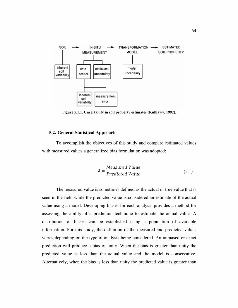
64

Figure 5.1.1. Uncertainty in soil property estimates (Kulhawy, 1992).

5.2. General Statistical Approach

To accomplish the objectives of this study and compare estimated values

with measured values a generalized bias formulation was adopted:

(5.1)

The measured value is sometimes defined as the actual or true value that is

seen in the field while the predicted value is considered an estimate of the actual

value using a model. Developing biases for each analysis provides a method for

assessing the ability of a prediction technique to estimate the actual value. A

distribution of biases can be established using a population of available

information. For this study, the definition of the measured and predicted values

varies depending on the type of analysis being considered. An unbiased or exact

prediction will produce a bias of unity. When the bias is greater than unity the

predicted value is less than the actual value and the model is conservative.

Alternatively, when the bias is less than unity the predicted value is greater than

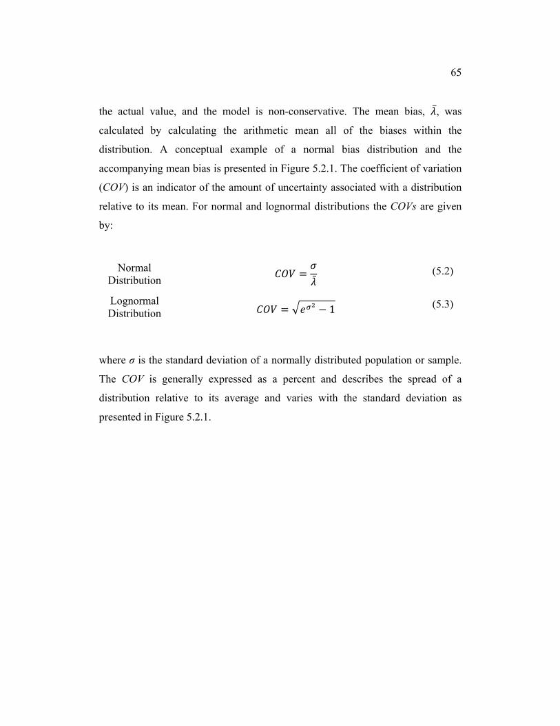
65

the actual value, and the model is non-conservative. The mean bias, , was

calculated by calculating the arithmetic mean all of the biases within the

distribution. A conceptual example of a normal bias distribution and the

accompanying mean bias is presented in Figure 5.2.1. The coefficient of variation

(COV) is an indicator of the amount of uncertainty associated with a distribution

relative to its mean. For normal and lognormal distributions the COVs are given

by:

where σ is the standard deviation of a normally distributed population or sample.

The COV is generally expressed as a percent and describes the spread of a

distribution relative to its average and varies with the standard deviation as

presented in Figure 5.2.1.

Normal Distribution

(5.2)

Lognormal Distribution 1 (5.3)

66

Figure 5.2.1. Conceptual visualization of the defined bias assuming a normal distribution.

5.3. Development of Soil Profiles

Soil profiles for each case history were digitized and a standardized

process for extracting data was developed to accommodate the varying soil types,

stratigraphy, and subsurface investigation procedures. The soil parameters

estimated were extracted from soil profile data to a depth greater than 2B beneath

the base of the footing depth. A discretized soil profile with layer thicknesses of

0.15 meters was developed to minimize the effect of sampling variation on the

soil parameters. From the available soil information, provided at defined depths,

the soil profile was linearly interpolated with depth. In some cases, the subsurface

investigation was not sufficient enough to characterize the soil mobilized during

0 0.5 1 1.5 2

Pd

f

Bias

σ1

σ2

67

load testing. Soil parameters from the above or below soil layer were used in

these instances.

5.4. Estimation of Selected Soil Parameters

The soil parameters required, such as undrained shear strength, OCR, and

elastic modulus were occasionally provided in a case history. In cases where this

soil data was not provided, well established correlations and approximations were

employed to approximate soil parameters. Where possible the selection of

correlations was calibrated to available data to mitigate variability.

5.4.1. Undrained Shear Strength

The majority of case histories provided vane shear strength test (VST) data

to estimate undrained shear strength of the soil profile. Bjerrum (as discussed in

Ladd, et al., 1977) found that undrained shear strengths from the VST should be

corrected for PI according to Figure 5.4.1, and where the vane shear strength is

given as:

(5.4)

where suField is the undrained shear strength in the field, suVST is the undrained

shear strength given by the test, and μVST is the Bjerrum correction factor and is

based on PI.

Das (2011) expressed the Bjerrum correction factor, μVST, Figure 5.4.1

numerically as:

68

1.7 0.54 (5.5)

The correction factor presented by Das (2011) exhibits a large amount of

transformation variability, as shown by the scatter in the data used to develop this

correlation. By visual inspection of Figure 5.4.1, the estimated error of the VST

correction factor is approximately ± 25%; thus, when compounded with inherent

soil variability, this correlation may produce large variations in the undrained

shear strengths.

Tand (1986) provided cone tip resistance data from CPT explorations and

unconsolidated undrained (UU) triaxial tests at selected depths. The undrained

shear strength was correlated to CPT using the procedure given by Kulhawy and

Mayne (1990):

where suCPT is the undrained shear strength correlated from CPT, qc is the cone tip

resistance and Nk is the cone factor (analogous to bearing capacity factor, Nc),

which can vary between 11 and 25, depending on cone and soil type (Das, 2011).

(5.6)

69

Figure 5.4.1. VST correction factor based on PI, after (Kulhawy & Mayne, 1990).

The bearing capacity factor was approximated by rearranging Equation

(5.6) and setting suCPT equal to the undrained shear strength, suUU from UU triaxial

tests, which is given by:

The use of Equation (5.7) indicates that the cone factor is directly related

to the undrained shear strength; as such, the cone factor will contain the inherent

spatial and measurement uncertainty associated with it. As a result the Nk value

varied with depth. For this analysis a bearing capacity factor of 25 was selected as

(5.7)

70

the minimum of the values calculated over the soil profile depth and may present

the largest source of uncertainty in the estimation of undrained shear strength.

5.4.2. Overconsolidation Ratio

Five case histories provided information regarding preconsolidation

pressure, ’p, or OCR. To select the appropriate correlation to approximate OCR

for other case histories, the OCR profiles for these five case histories were

statistically compared to the results of four correlations: Larsson (1980), Wood

(1983), Stas and Kulhawy (1984), and Kulhawy and Mayne (1990). Each

correlation is presented in Table 5.4.1 and the results of the statistical approach

are presented in Table 5.4.2.

Table 5.4.1. Empirical OCR correlations used in statistical approach to estimate OCR

profiles.

Larsson (1980) 0.08 0.055 ∗ ′ (5.8)

Wood (1983) 10. ∗

(5.9)

Stas & Kulhawy (1984) ′

∗ 10 . . ∗(5.10)

EPRI (1990) 3.22′ (5.11)

71

The correlation selected for use in this analysis was Kulhawy and Mayne

(1990) as it produced the mean bias nearest to unity with the smallest standard

deviation. This correlation is given by:

3.22′

(5.12)

Equation (5.12) was applied to case histories where VST data was

provided to approximate OCR. A separate correlation was selected for case

histories that conducted other in-situ tests. The preconsolidation profile for Tand

(1986) was correlated from CPT data using Kulhawy and Mayne (1990), given

by:

′ 0.33′

(5.13)

where qT is the cone tip resistance corrected for pore water pressure. The

substitution of Equation (5.13) into Equation (2.19) produced the assumed OCR

profile.

Table 5.4.2. Statistical results of OCR comparison.

Larsson (1980)

Wood (1983)

Stas & Kulhawy (1984)

EPRI (1990)

Mean Bias 3.12 1.94 1.21 0.79

Standard Deviation 4.88 3.06 2.20 0.59

72

For six case histories, the saturated unit weight of the soil, γsat, was

assumed in order to develop the effective stress profile. Table 5.4.3 presents

approximate saturated unit weights based on consistency and OCR.

Table 5.4.3. Expected ranges in saturated unit weight of clay soils based on OCR, from

(Stuedlein, 2010)

5.4.3. Initial Undrained Young’s Modulus

The relationship suggested by Duncan and Buchignani (1987) was used to

approximate the initial undrained Young’s modulus of the soil which is given by:

where the K-factor presented in Figure 5.4.2 is based on OCR and PI. Additional

information regarding testing procedures or strain level measurements was not

provided along with Figure 5.4.2. By visual inspection of Figure 5.4.2, the K-

factor exhibits significant uncertainty. As a result, a standardized procedure to

calculate the K-factor was established. Figure 5.4.2 was digitized and values of

the K-factor were linearly interpolated between the solid lines based on PI.

OCR γsat

(kN/m3)

Very Soft to Soft 1 14 - 15 Medium Stiff 1.2 – 1.5 15 - 17

Stiff 1.5 - 4 17 - 19 Very Stiff 4 - 20 19 - 21

Hard 20+ 22

(5.14)

73

Figure 5.4.2. Variation in K-factor based on OCR and PI, from (Duncan & Buchignani,

1987).

5.5. Load Test Database

The load test database presented in Table 4.3.1 consists of 12 case

containing 30 individual footing load tests on soils ranging from highly plastic

silts to normally consolidated soft clays. There was only a single soil profile

where the soil stress history corresponded to normally consolidated conditions.

The database consisted of 13 square foundations and 17 circular footings. Two

footings rested on the ground surface while 28 had some amount of embedment.

74

Foundation materials consisted of steel and concrete with 14 footings comprised

of steel and 16 of reinforced concrete.

The estimation of bearing capacity requires the consideration of the

undrained shear strength, su, as discussed in Chapter 2. The relationship between

undrained shear strength and stiffness parameters is well-known and is discussed

in Chapter 5. Pertinent soil parameters and additional values used in this analysis

are compiled in Table 5.5.1. The methods to develop the estimated undrained

shear strength and estimated initial Young’s modulus are discussed in Chapter 5.

Additional parameters presented in Table 5.5.1 are discussed in Chapter 7.

75

Table 5.5.1. Summary of load test database of shallow footing on clay.

Test ID Beq

a (m)

su,estb

(kPa) su,ext

c

(kPa) qd

(kPa)qult

e (kPa)

q*ultf

(kPa) Ei,est

g (MPa)

Ei,bch

(MPa)BB - 1 1.18 20 21 24.4 191 177 1.6 16.3 BB - 2 1.02 20 25 24.4 196 213 2.0 14.8 BB - 3 0.85 20 26 24.4 204 228 2.1 12.7 BB - 4 0.76 21 25 24.4 209 227 2.1 17.4 BB - 5 0.68 21 30 24.4 211 271 2.5 12.6 GG - 1 1.03 44 41 11.3 347 313 18.2 11.0 ON - 1 0.59 20 62 6.4 162 415 27.0 10.0 ON - 2 0.49 20 31 6.4 170 221 14.1 6.3 ON - 3 0.34 20 42 6.4 172 342 17.1 8.7 OB - 1 0.46 74 58 39.7 742 560 13.7 6.2 OB - 2 3.50 108 77 11.8 734 502 11.59 42.6 CM - 1 0.87 139 87 0.0 858 539 34.4 33.0 HA - 1 1.13 48 71 0.0 298 440 19.7 31.7 HA - 2 1.13 48 76 0.0 298 518 21.0 27.5 RB - 1 0.30 38 29 0.0 231 180 4.6 4.7 TT - 1 0.58 44 89 23.9 429 813 16.6 19.2 TT - 2 0.58 44 97 23.9 429 882 18.0 16.8 TT - 3 0.58 44 80 23.9 429 734 15.0 17.6 TT - 4 0.58 45 42 23.9 436 382 11.1 8.0 TT - 5 0.58 45 25 23.9 436 225 6.6 10.0 TT - 6 0.58 67 112 25.9 640 1021 13.1 14.5 TT - 7 0.58 67 105 25.9 640 963 12.3 20.2 TT - 8 0.58 67 92 25.9 640 844 10.8 18.0 BH - 1 2.48 21 30 12.48 160 205 20.7 5.5 BD - 1 0.68 20 31 10.6 175 262 3.9 14.5 BD - 2 0.68 20 44 10.6 175 365 5.4 6.8 BL - 1 2.26 20 15 25.8 186 120 11.4 10.9 TS - 1 0.76 70 93 12.0 582 754 21.0 24.7 TS - 2 0.76 70 95 12.0 582 774 21.6 21.6 TS - 3 3.09 85 92 0.0 526 568 20.9 12.9

a equivalent footing diameter e estimated bearing capacity

b estimated undrained shear strength f bearing capacity extrapolated using hyperbolic modelc extrapolated undrained shear strength g estimated initial Young’s modulus

d effective surcharge at footing depth h back-calculated initial Young’s modulus

76

5.6. Summary of Methodology

The methodology used in this study focused on the development of soil

profiles and parameters from data extracted from the load test database. Data

provided from each case history was correlated to required soil parameters while

variability in the correlations was minimized using calibration techniques. The

uncertainty in prediction of soil parameters is likely quite large due to the

variation in the quality and consistency of the reported subsurface investigations.

Assessment of the uncertainty in prediction quality will be presented in the

subsequent sections.

77

Chapter 6: Uncertainty in Prediction of Bearing Capacity

6.1. Introduction

Uncertainties in the prediction of bearing capacity develop from inherent

spatial variability of the soil, uncertainties that stem from transformation of

measured soil parameters (e.g. PI to su), and errors within the design model. The

statistical approach outlined in Section 5.2 was conducted to assess the effects of

uncertainty in predicted bearing capacity using the bearing capacity formula and

extrapolations from load tests. Additionally, undrained shear strengths mobilized

during load testing were estimated by applying bearing capacity theory to bearing

pressure-displacement curves and compared to the estimated undrained shear

strength.

6.2. Application and Uncertainty of the Hyperbolic Model to Bearing

Pressure-Displacement Curves

A hyperbolic bearing pressure-displacement model was adopted in this

study to assess the bearing capacity of footings. This hyperbolic model is similar

to the Chin method (see Section 2.2.2), and allows the fitting of a hyperbolic

relationship to the q-δ curve using the following steps:

Step 1: Normalize displacements, δ, by the footing width, B, to produce a

pseudo-strain (δ/B) (Uzielli & Mayne, 2011).

Step 2: Divide the pseudo-strain by the applied bearing pressure (δ/B)/qapp at

the observed displacements.

Step 3: Plot the (δ/B)/qapp vs. the pseudo-strain to produce a transformed

representation of the q-δ behavior (e.g. Figure 6.2.1).

78

Step 4: Fit a linear trend to the transformed data ignoring initial points, as

appropriate (Figure 6.2.1).

Step 5: The fitted slope coefficient, C1, is inverted to provide the estimated

ultimate resistance, or bearing capacity.

The initial portion of the transformed curve is ignored as the information

at higher displacements is more representative of “capacity”. A transformed

bearing pressure-displacement curve is presented in Figure 6.2.1 and the

associated predicted and observed q-δ curve is presented in Figure 6.2.2. The

bearing capacity estimated from the resulting transformation is given by the

asymptote implied by the hyperbolic relationship (Kondner, 1963):

where C1 is the slope of the linear portion of the transformation. The bearing

resistance at a given displacement, q*app, calculated using the hyperbolic model:

where C2 is the intercept of the linear portion of the transformed curve presented

in Figure 6.2.1.

The application of the hyperbolic model requires judgment in the selection

of data pairs to be considered in the linear portion of the transformed curve. The

judgment typically is the responsibility of the designer and introduced additional

transformation uncertainty into the analysis. The bearing pressure bias, λq, which

is given as:

∗ 1 (6.1)

∗ (6.2)

79

where qapp is the observed bearing pressure at a given displacement and q*app is

defined in Equation (6.2).

Figure 6.2.1. Hyperbolic fitting method applied to footing load test TS-1.

The hyperbolic model was fitted to the pressure-displacement curves and

the bias was calculated for each q-δ pair in the database (termed point bias), as

well as averaged for a given q-δ curve in its entirety (termed averaged bias). The

0.00E+00

5.00E-05

1.00E-04

1.50E-04

2.00E-04

2.50E-04

3.00E-04

3.50E-04

0.00 0.05 0.10 0.15 0.20 0.25

Nor

mal

ized

Dis

pla

cem

ent/

Ap

pli

ed B

eari

ng

Pre

ssu

re, (δ/

B)/

q app

(1/k

Pa)

Normalized Displacement, δ/B

Linear Trend

Linear Portion

Discarded Points

∗ (6.3)

80

bearing pressure-displacement curves and corresponding transformed curves are

presented in Appendix B.

Figure 6.2.2. Fitted hyperbolic q-δ curve using method compared to that observed for

footing load test TS-1.

Histograms for the point and averaged biases are presented in Figure 6.2.3

and Figure 6.2.4, respectively; normal and lognormal distributions were fitted to

the bias data set for comparison. The mean and standard deviations of the

observed bias data sets were computed and used to produce a theoretical fitted

distribution. The first step in fitting a distribution is to rank the biases from lowest

0

100

200

300

400

500

600

700

800

0 50 100 150 200

Ap

pli

ed B

eari

ng

Pre

ssu

re(k

Pa)

Displacement, δ (mm)

Observed load-disp. data

Predicted using hyperbolic model

81

to highest magnitude and calculate the cumulative probability associated with

each bias value, given by (Allen, et al., 2005):

where i is the rank of each bias and n is the number of observations. A cumulative

distribution function (CDF) can be developed by plotting the data pairs of

cumulative probability of occurrence and ranked bias. The probability is used to

calculate the standard normal variate, Zi, which is given by:

where Φ-1 returns the standard normal variate. The bias value for a theoretical

normal distribution may be calculated using (Allen, et al., 2005):

where and σ are the mean and standard deviation of the bias data set. Data

points that deviate from the distribution calculated using Equation (6.6) indicate a

poor representation of the normal distribution (Figure 6.2.4). The lognormal

distribution is often used to approximate sample distributions and can be

computed using (Allen, et al., 2005):

1

(6.4)

(6.5)

∗ (6.6)

∗ (6.7)

82

where ln and σln are the log mean and log standard deviation of the dataset,

respectively. In some cases a dataset may not be entirely represented by a normal

or lognormal distribution. In these instances, and where some portion of the

distribution must be captured more accurately than other portions, an adjusted or

fit-to-tail distribution may be required; this fitting procedure is discussed in more

detail in Chapter 8.

Allen et al. (2005) recommended that good agreement between theoretical

and observed bias data when a COV of the theoretical model is less than

approximately 20 to 30 percent. The mean bias is defined as the average bias of

the entire distribution and the COV is calculated using Equation (6.3). Mean

bearing pressure biases and COVs are summarized statistically in Table 6.2.1.

Table 6.2.1. Statistical summary of biases for the fitting of the hyperbolic model to observed

q-δ curves.

Bearing Pressure Point Bias Bearing Pressure Averaged Bias

Mean, COV Mean, COV

1.133 41.3% 1.125 22.1%

where:

1 (6.8)

ln 0.5 ∗ (6.9)

83

Figure 6.2.3 presents the histogram and CDF of each bearing pressure-

displacement point, which totals 240 points, and also displays the fitted

theoretical distributions. The normal and lognormal distributions are represented

by the solid and dashed lines, respectively. These distributions may provide a

mean bias ( = 1.13), but do not adequately fit the trend of the bearing pressure-

displacement distribution. The large variability (COV = 41.3 percent) stems from

the tendency for the hyperbolic model to under-predict the initial portion of the q-

δ curve. The first three q-δ points of Figure 6.2.2 provide an example of the

general trend of the model to under-predict q*app for a given displacement at small

displacements, which produces a bias value greater than unity.

Figure 6.2.3. Sample and fitted distributions of point biases for the observed and fitted

bearing pressures and displacements.

Bias

Densi

ty

0.0 1.0 2.0 3.0

01

23

0.0 1.0 2.0 3.0

0.0

0.2

0.4

0.6

0.8

1.0

Bias

CD

F

Normal distribution = solid line, lognormal distribution = dashed line

84

Figure 6.2.4 presents a histogram, containing 30 data bias points, of the

averaged bearing pressure-displacement points and the corresponding fitted

theoretical distributions. By visual inspection of Figure 6.2.3 and Figure 6.2.4 the

point and averaged bearing pressure model were better approximated by

lognormal distributions. Table 6.2.1 indicates that the mean of the averaged bias

was relatively unchanged when compared to that of the point bias ( = 1.13);

however, the variability in the bearing pressure model was significantly reduced

(COV = 22 percent).

The results of the analyses ( = 1.13) indicate that the hyperbolic model

sufficiently predicts the bearing pressure-displacement behavior of shallow

footings in the database and indicates that the actual bearing pressure tends to be

slightly greater on average than those predicted. The 19 percent reduction in

variability that occurs after the point biases are averaged, indicates that

approximately half of the variability associated with the prediction stems from

point to point comparison of the hyperbolic model. The majority of the variability

may be attributed to the lack of fit at the initial portion of the q-δ curve which can

be seen in Figure 6.2.2. This uncertainty likely stems from the initial points that

were discarded during the transformation to capture the bearing pressure at higher

displacements. Nonetheless the hyperbolic model adequately predicts the bearing

pressure-displacement behavior of shallow foundations on undrained clay.

85

Figure 6.2.4. Sample and fitted distributions of averaged biases for the observed and fitted

bearing pressures and displacements.

6.3. Uncertainty in Bearing Capacity using Estimated Undrained Shear

Strengths

The bearing resistance of soil develops as its strength is mobilized along

an assumed shearing plane. The assumed shearing plane is presented in Figure

2.2.1 for footings on clay. The bearing capacity associated with the assumed

failure surface can be approximated using the general bearing capacity formula

[see Equation (2.6)]. The estimated bearing capacity of clays primarily depends

on the undrained shear strength. The use of a single soil parameter reduces the

computational and investigative effort required to estimate bearing capacity.

Bias

Dens

ity

0.5 1.0 1.5 2.0 2.5 3.0

01

23

45

6

0.5 1.0 1.5 2.0 2.5 3.0

0.0

0.2

0.4

0.6

0.8

1.0

Bias

CD

F


86

Therefore, the resulting prediction depends on the variability of that soil

parameter and the bearing capacity model uncertainty. The effects of these

sources of uncertainty/variability are investigated herein.

6.3.1. Bearing Capacity Predicted Using Estimated Undrained Shear Strengths

Bearing capacities were predicted using the general bearing capacity

formula, Equation (2.6), with bearing capacity factors given in Table 2.2.2, and

depth and shape factors given in Table 2.2.3. These were compared to observed

bearing capacities (i.e. extrapolated) developed from the hyperbolic model using

biases. The bias in bearing capacity, λBC, is given as:

where q*ult is the extrapolated bearing capacity and qult is the bearing capacity

predicted using the general bearing capacity formula. The use of the same

procedure as outlined in the previous section to fit normal and lognormal

distributions facilitated determination of the distribution of the bearing capacity

biases. A summary of the results of the fitting procedure and data analysis is

presented in Table 6.3.1.

The mean bias of the bearing capacity model ( = 1.30) indicates that

the bearing capacity predicted using the general bearing capacity formula under-

predicts observed, or extrapolated bearing capacity. The high variability (COV =

39 percent) indicates a significant amount of uncertainty. Figure 6.3.1 presents the

histogram and CDF distributions of the bearing capacity comparison and the

corresponding fitted normal and lognormal distributions. Visual inspection of the

distribution shows that the bearing capacity distribution is more lognormally

∗

(6.10)

87

distributed. It is also important to note that the normal distribution produces

negative bearing capacity values which do not exist. Thus, a lognormal

distribution better represents the bearing capacity bias distribution.

Figure 6.3.1. Sample and fitted distributions of the biases for the observed and predicted

bearing capacity.

6.3.2. Effects of Surcharge on Bearing Capacity

Engineers typically neglect the surcharge component of bearing capacity,

providing a small amount of conservatism by reducing the available bearing

capacity. The effect of neglecting the surcharge was analyzed and compared to

the bearing capacity extrapolated from q-δ curves by computing biases. The bias

calculation for bearing capacity without surcharge, λoBC is given as:

Bias

De

nsi

ty

0.0 0.5 1.0 1.5 2.0 2.5

0.0

0.2

0.4

0.6

0.8

1.0

1.2

0.0 0.5 1.0 1.5 2.0 2.5

0.0

0.2

0.4

0.6

0.8

1.0

Bias

CD

F


88

where N’q, λqs, and λqd are equal to unity according to Table 2.2.3 and all other

symbols are previously defined.

The term of Equation (6.12) is typically referred to as the

surcharge component and only accounts for approximately 15 percent or less of

the bearing capacity for shallow foundations. A statistical comparison of the

bearing capacity biases with and without surcharge was conducted to quantify the

effect of surcharge on bearing capacity. Table 6.3.1 presents a summary of the

comparison and indicates that the incorporation of surcharge provides a better

prediction of the bearing capacity. Removing the surcharge component from the

bearing capacity formula reduced the mean predicted capacity by approximately 5

percent. Thus, providing a larger estimate of bearing capacity using the traditional

method ( = 1.30) compared to the method neglecting surcharge ( = 1.37)

with little change in the variability.

Table 6.3.1. Effect of surcharge on bearing capacity estimate.

Mean Bias 1.30 1.37

COV 39% 38%

∗

(6.11)

where: (6.12)

89

6.3.3. Evaluating Predicted Bearing Capacity for Dependency

The development of a model to predict bearing capacity must take into

account the dependency, or correlation, that exists between the observed and

predicted (nominal) capacities. A zero slope test is often performed to determine

the dependency between two populations by using linear regression techniques to

calculate the slope and intercept of a trend line. The null hypothesis, or primary

argument, of the zero slope test is that the slope of the linear trend is equal to

zero. The slope of the trend line is divided by the standard error to produce a test

statistic, t, which can be compared to the Student’s t distribution to calculate the

probability that the null hypothesis is true. Figure 6.3.2 presents the regression of

nominal (or predicted) bearing capacity against the bias. The slope, b1, of the

regression is -0.0007 while the intercept, b2, is 1.57; the corresponding test

statistic and probability against the null hypothesis, p, are -1.571 and 0.127,

respectively. This indicates that the probability that the slope of the regression is

not equal to zero is approximately 13 percent.

A significance level, α, is defined as the acceptable level of probability

against the null hypothesis (i.e. the maximum p-value allowed). Using a typical

significance level of 0.05 is acceptable for this analysis. Based on these results,

the p-value is greater than our significance value and the slope of the regression

line between the nominal capacity and bias is statistically equivalent to zero (i.e.

we fail to reject the null hypothesis). Thus, it is concluded that the capacity model

does not need to be adjusted to eliminate dependence.

90

Figure 6.3.2. Traditional bearing capacity versus bearing capacity bias.

6.3.4. Effect of Undrained Shear Strength on Prediction of Bearing Capacity

using Monte Carlo Simulation

The Monte Carlo method of simulation is a generic numerical method that

uses many random variables to produce and extrapolate the statistics of a system.

This study used Monte Carlo simulations to evaluate the effect on variability in su

on the bearing capacity of a typical footing. Random variables incorporating the

variability of the undrained shear strength and the uncertainty of the bearing

capacity model were simulated to populate the predicted bearing capacity

distribution and draw inferences about the effect of uncertainty on the bounds of

capacity. The application of the Monte Carlo simulation involves the following

steps (Jones, et al., 2002):

0.0

0.5

1.0

1.5

2.0

2.5

3.0

0 100 200 300 400 500 600 700 800 900 1000 1100

Bea

rin

g C

apac

ity

Bia

s

Traditional Bearing Capacity, qult

Traditional BearingCapacity DataLinear Regression

Mean Bias

λ = 1.57 - 0.0007qult

91

1. Selection of a model that will produce a deterministic solution to a

problem of interest;

2. Decisions regarding which input parameters are to be modeled

probabilistically and the representation of their variability in terms of

probability distributions;

3. Generation of multiple random estimates of input parameters that fit the

appropriate probability distributions and are consistent with the known

or estimated correlation between input parameters;

4. Repeated determination of the deterministic model to develop a

probability density function from which useful statistics can be

approximated.

To assess the effects of uncertainty in undrained shear strength and

bearing capacity model, a typical footing of 2 meters in equivalent diameter with

an embedment depth of 1 meter was modeled. The selected clay soil was

modeled using a saturated unit weight of 17 kN/m3 and an undrained shear

strength of 40 kPa. For this scenario, the estimated bearing capacity is 313 kPa

using the general bearing capacity formula. To assess the impact of variability in

undrained shear strength, 12 Monte Carlo simulations each using 50,000 random

estimates of su were performed. To assess the effect of uncertainty in a bearing

capacity prediction model, Monte Carlo simulations were separated into two cases

with 6 simulations each (Table 6.3.2): Case A neglected the nominal bearing

capacity model uncertainty, and Case B incorporated model uncertainty (Table

6.3.2). To assess the effect of variability in undrained shear strength, the COV in

the undrained shear strength, COVsu, was varied at 5, 10, 20, 30, 50 and 100

percent for each of the cases.

92

Table 6.3.2. Monte Carlo simulations conducted to assess uncertainty.

Case A Case B

Number of Monte Carlo Simulations

6 6

Model Uncertainty BC = 1.0 COV = 0%

BC = 1.30 COV = 39%

COVsu 5, 10, 20, 30, 50, 100%

To compound the uncertainty associated with the undrained shear strength

with the model uncertainty, a first order approach (Allen, et al., 2005) was

adopted:

∗ (6.13)

(6.14)

where is the total bias and COVfinal is the total coefficient of variation.

Cumulative density (CDF) plots of the results were generated to assess the

impact of su variability. The undrained shear strength distribution was assumed to

be lognormal based on work conducted by Phoon and Kulhawy (1999) and Jones

et al. (2002). Table 6.3.3 summarizes the results of Case B. Prior to the

incorporation of model uncertainty, the uncertainty associated with the prediction

of bearing capacity was limited to the variability in the undrained shear strength.

As a result a summary of that analysis is not presented in table form because the

COVsu will be equal to COVBC. As such, COVsu is termed the initial COV while

COVBC is labeled as the resulting variability in bearing capacity prediction due to

93

the incorporation of the model uncertainty. At an initial variability of 5 percent

the resulting uncertainty in bearing capacity increased to 39 percent, whereas at

an initial variability of 100 percent, COVBC increased to 109 percent. This

indicates that the effect of model uncertainty is smaller at larger COVsu.

Table 6.3.3. Summary of bearing capacity distribution resulting from Case B Monte Carlo

simulations.

Undrained Shear Strength COVsu

5% 10% 20% 30% 50% 100%

Standard deviation in Bearing

Capacity(kPa)

123 126 139 156 202 340

COV 39% 40% 44% 50% 64% 109%

In general, as the COVsu ranges from 5 to 100 percent, COVBC ranged

from 39 to 109 percent. The reduction in ranges indicates that incorporation of

model uncertainty reduced the effect of variability in undrained shear strength on

bearing capacity prediction. However, it should be noted that the overall

uncertainty was increased and only the differences in ranges was discussed herein.

Figure 6.3.3 presents CDFs of the Monte Carlo simulations for Case A;

for the simulation where the COVsu = 5 percent, a tight band of bearing capacities

is predicted. For the simulation with a COV of 100 percent, a large range of

predicted bearing capacities was produced, with the largest and smallest estimates

being 25 kPa and 7400 kPa, respectively. Dividing the largest prediction of

bearing capacity resulting from Case A for COVsu of 100 percent (7400 kPa) and

dividing it by the largest prediction for a COVsu of 5 percent (384 kPa) produces

an increase of about 1900 percent. Repeating the same methodology for Case B

yields an increase of 700 percent (Table 6.3.4). The results of this comparison

94

show that the incorporation of model uncertainty greatly increases the range of

predicted bearing capacities.

Table 6.3.4. Comparison of largest and smallest possible bearing capacities.

Case A Case B COV Largest Capacity

100% 7400 10400 5% 380 1480

% Change 1900 700

Figure 6.3.3. CDFs of bearing capacity showing variations in undrained shear strength for

Case A.

0%

10%

20%

30%

40%

50%

60%

70%

80%

90%

100%

0 200 400 600 800 1000 1200

Pro

bab

ilit

y of

Non

-exc

eed

ance

Bearing Capacity (kPa)

COV = 5%

COV = 10%

COV = 20%

COV = 30%

COV = 50%

COV = 100%

95

Figure 6.3.4. CDFs of bearing capacity showing variations in undrained shear strength for

Case B.

By visual inspection of Figure 6.3.3 and Figure 6.3.4, the prediction of the

median bearing capacity (probability of occurrence = 50%) reduces by

approximately 80 kPa as COVsu increases from 5 to 100 percent. A comparison

between the CDFs of the initial and traditional model for a COVsu of 30% is

presented in Figure 6.3.5. The vertical line approximates the predicted bearing

capacity using the general bearing capacity formula (313 kPa) and approximately

45 percent of the predicted bearing capacities are greater than the deterministic

prediction.

0%

10%

20%

30%

40%

50%

60%

70%

80%

90%

100%

0 200 400 600 800 1000 1200

Pro

bab

ilit

y of

Non

-exc

eed

ance


COV = 5%COV = 10%COV = 20%COV = 30%COV = 50%COV = 100%

Case B

96

Figure 6.3.5. Comparison of predicted bearing capacity CDFs at a COV of 30%.

6.4. Back-Calculation of Undrained Shear Strength using the Hyperbolic

Model

General bearing capacity formulas can be applied to bearing pressure-

displacement curves to approximate mobilized undrained shear strengths at a

given displacement. Mobilized undrained shear strengths were calculated by

rearranging Equation (2.6) and substituting the bearing resistance from the

bearing pressure-displacement curves for each displacement. Hence, the

mobilized undrained shear strength can be expressed as:

0%

10%

20%

30%

40%

50%

60%

70%

80%

90%

100%

0 150 300 450 600 750 900 1050 1200

Pro

bab

ilit

y of

Non

-exc

eed

ance


Case A

Case B

Greater than deterministic

97

where all values are previously defined and N’q, λqs, and λqd are equal to unity (see

Table 2.2.3).

The surcharge component, qN’qλqsλqd, develops from the weight of soil

above the foundation depth, q, resisting the upward motion of the mobilized soil

in the Rankine Passive Zone (see Section 2.2.1) as a load is applied. When back-

calculating the undrained shear strength from the general bearing capacity

formula, the strength of interest is produced from soil mobilization along the

failure surface. As a result the surcharge component can be removed, because it

only provides resistance in the form of vertical pressure. However, the additional

soil above the foundation depth does increase the length of the failure plane. This

is accounted for in the depth embedment factor, λcd, applied to the cohesion

component of the general bearing capacity formula. With these assumptions,

equation (6.15) reduces to:

The application of Equation (6.16) to q-δ curves produces mobilized

undrained shear strength (su,mob-δ) curves that are similar in shape to the q-δ

curves. An example for load test TS-1 is presented in Figure 6.4.1. The hyperbolic

model can be used to extrapolate undrained shear strengths (i.e. measured). These

were compared to the undrained shear strengths estimated in Chapter 5 which are

being treated as the predicted value for this comparison. Biases were calculated

by:

, (6.15)

, (6.16)

98

where su,est and su,ext are the estimated and extrapolated undrained shear strengths,

respectively. A summary of the comparison is presented in Table 6.4.1 and

indicates that the estimated undrained shear strength slightly under-predicts

observed (extrapolated) undrained shear strengths ( = 1.10) when compared to

estimated values.

Figure 6.4.1. Example of mobilized undrained shear strength curve data for load test TS-1.

0

10

20

30

40

50

60

70

80

90

0.00 0.05 0.10 0.15 0.20

Mob

iliz

ed U

nd

rain

ed S

hea

r S

tren

gth

, su

.mob

(kP

a)

Normalized Displacement, δ/B

From observed loaddisplacement data

Predicted fromhyperbolic model

,

, (6.17)

99

The variability in the fitted distributions (COV = 39%) likely develops

because the extrapolation produces an undrained shear strength averaged over the

entire assumed shear failure plane while the estimated undrained shear strength

was averaged only over the equivalent footing width, Beq. The application of the

general bearing formula to back-calculate the undrained shear strength provides a

method of estimating the undrained shear strength from footing load tests.

However, by applying the general bearing formula and the hyperbolic model to

extrapolate su,mob-δ curves, the uncertainty for that model or correlation must also

be taken into account when estimating the undrained shear strength. The bearing

capacity model uncertainty was accounted for using Equation (6.13) and Equation

(6.14) discussed in Section 6.3.4.

A mean compounded undrained shear strength bias, , and COV were

estimated and presented in Table 6.4.1. The reduced from 1.10 to 0.85 while

the COV increased from 39 to 55 percent. This indicates that the estimated

undrained shear strengths are lower than the actual (extrapolated) undrained shear

strengths. However, when the model bias and uncertainty are incorporated into

the extrapolation, the estimated undrained shear strengths actually become greater

than those predicted and the estimated undrained shear strengths become non-

conservative.

The procedure outlined in Section 6.3 was followed to develop fitted

distributions to the undrained shear strength distribution and is presented in

Figure 6.4.2. Figure 6.4.2 shows that the undrained shear strength distribution

provides a better fit to a lognormal distribution, which validates the initial

assumption discussed in Section 6.3.1.

100

Table 6.4.1. Summary of undrained shear strength comparison.

Undrained Shear Strength Bias

Mean, COV

Observed 1.10 39%

Compounded 0.85 55%

Figure 6.4.2. Distribution of undrained shear strength bias with fitted distributions.

6.5. Summary

Bearing capacities were extrapolated by applying a hyperbolic model to q-

δ curves produced from footing load tests and were compared to capacities

Bias

Densi

ty

0.0 1.0 2.0 3.0

0.0

0.5

1.0

1.5

2.0

2.5

3.0

0.0 1.0 2.0 3.0

0.0

0.2

0.4

0.6

0.8

1.0

Bias

CD

F


101

predicted using the general bearing capacity formula. A statistical model was

developed to assess the effect of variability in undrained shear strength on bearing

capacity. The application of general bearing capacity formulas to q-δ curves

permitted the back-calculation of mobilized and extrapolated undrained shear

strengths and comparison to estimated strengths. The conclusions stemming from

the work presented in this chapter include:

1. The hyperbolic model accurately predicts q-δ curves produced by footings

on clay with a relatively low amount of uncertainty ( = 1.13, COV = 22

percent).

2. Bearing capacity predicted using the general bearing capacity formula that

incorporates surcharge under-predicts the actual (extrapolated) bearing

capacity with a relatively high amount of uncertainty ( = 1.30, COV =

39 percent).

3. Subtraction of surcharge effects from the general bearing formula reduces

the available bearing capacity by approximately 5 percent and produces a

slightly less accurate prediction ( = 1.37, COV = 39 percent).

4. Predicted bearing capacities are considered to be statistically independent

from the actual (extrapolated) bearing capacities (two sided p-value =

0.13).

5. Model uncertainty greatly increased the variability in bearing capacities

calculated using the general bearing capacity formula.

6. The use of su,mob-δ curves predicts the estimated undrained shear strengths

relatively accurately ( = 0.85), although there is also a relatively high

amount of uncertainty (COV = 55 percent).

102

Chapter 7: Uncertainty in Prediction of Displacements

7.1. Introduction

Prediction of immediate displacements of shallow foundations is primarily

limited to elasticity-based models, which do not account for the soil nonlinearity.

As a result, the combination of inherent soil variability, design parameter

variability, and design model error may produce inaccurate estimates of

immediate settlement estimates. This study assessed the application of a nonlinear

hyperbolic model to improve the prediction of immediate displacements of

foundations on clay, and the uncertainty associated with both the proposed model

and elasticity-based predictions.

7.2. Development of Proposed Model

The Duncan-Chang hyperbolic model (Duncan & Chang, 1970) and is a

convenient and widely accepted nonlinear soil constitutive model. The model is

discussed in detail by Duncan et al. (1980). The Duncan-Chang model expresses

the development of the principal stress difference as a function of axial strain,

initial Young’s modulus, and effective confining pressure. The stress path that

develops below a footing during a load test is similar to an undrained triaxial test

compression stress path (Stuedlein & Holtz, 2010). The available strength beneath

the footing is defined by the effective stress path. The failure criterion is defined

as the point at which the principal stress difference exceeds the available shear

strength. For stress paths the ultimate strength of soil is defined by ultimate

principal stress difference. Setting the ultimate principal stress difference equal to

the undrained shear strength produces the failure criterion:

103

where (σ’1 - σ’3)ult is the principal stress difference at failure.

Work by Kondner (1963) involving uniaxial compression and direct shear

tests indicated that a two-constant hyperbolic model could sufficiently capture

stress-strain behavior of a cohesive soil, as described in Chapter 6. Elasticity-

based prediction methods use a single elastic modulus, as discussed in Section

2.5, whereas the Duncan-Chang model updates the modulus with applied stress as

presented in Figure 7.2.1. The original model developed by Kondner (1963) is

given as:

where ε is the axial strain and Ein is the initial undrained Young’s modulus

(Figure 7.2.1), which depends on confining stress. For drained tests, this value

must be updated with increasing confining stress; however, in undrained tests the

initial undrained Young’s modulus remains constant (Duncan, et al., 1980).

The displacement response of each footing in the load test database was

modeled using the Duncan-Chang model and elasticity theory. The distribution of

stress was generated using elastic stress distributions for rigid footings in

undrained conditions. Thus the relevant parameters are the elastic modulus and

Poisson’s ratio, νs, which is equal to 0.5 for undrained loading of cohesive soils.

During loading, the change in vertical and horizontal stresses, Δσ1 and Δσ3, can be

redefined as the change in vertical and radial stresses, Δσv and Δσr, respectively,

′ ′ 2 (7.1)

1

′ ′

(7.2)

104

by assuming that square footings can be treated as equivalent circles (Davis &

Poulos, 1972). The principal stress difference is therefore given by:

Figure 7.2.2 presents the normalized elastic stress distribution, Δσ/qapp,

that develops beneath the center of a circular footing as a function of depth, z,

normalized by the footing radius, r. The principal stress difference reaches a

maximum value of approximately 0.18 at a normalized depth of unity and

diminished to 0.1 at a normalized depth of about 2.2.

Figure 7.2.1. Hyperbolic model stress-strain behavior.

(7.3)

105

Figure 7.2.2. Normalized elastic stress distributions beneath a rigid footing.

The displacement beneath a footing is calculated by rearranging Equation

(7.2) (Stuedlein & Holtz, 2010) to include the summation of the strains computed

using the Duncan-Chang model:

0

1

2

3

4

5

6

7

8

9

10

0.0 0.1 0.2 0.3 0.4 0.5 0.6

Nor

mal

ized

Dep

th (

z/r)

Normalized Stress Distribution (Δσ/q)

Vertical,

Radial,

Difference,

Δσv

Δσr

Δσvr

106

and computing strains at incremental depths, ΔZj. As the axial strain increases the

stress-strain behavior approaches an asymptote controlled by the principal stress

difference at failure, (σ’1 - σ’3)ult.

Substitution of Equations (7.1) and (7.3) into Equation (7.4) produces an

expression for displacement based on the integration of strains over the entire

depth of interest. This study considered the depth of 4r or 2B for integration of

strains and the displacement resulting from an applied load, δ, can be calculated

using:

7.3. Application and Validity of the Duncan-Chang Model

The proposed Duncan-Chang model can be applied to load-deformation

behavior beneath a footing due to the similarity in the loading condition to a

triaxial compression test. The application of the Duncan-Chang model to footing

load tests requires that the undrained shear strength and initial undrained Young’s

modulus be known for each layer. This is rare in design situations and as a result

the pertinent soil parameters (su, OCR and PI) were averaged over a depth of Beq

(see Chapter 2) below the footing where the majority of the large strains develop.

′ ′

, 1′ ′′ ′

(7.4)

1 2

(7.5)

107

There are several factors that affect the validity of the application of the

Duncan-Chang model. The selection of a single initial Young’s modulus assumes

that the soil remains undrained throughout the entire load test. In a drained test the

initial Young’s modulus will change with change in effective stress based on

work conducted by Duncan and Chang (1970). An expression for the initial

Young’s modulus was developed based on numerous experimental triaxial tests

and is given as (Janbu, 1963):

where Pa is the atmospheric pressure with units matching to σ’3, KDun and n are

the modulus number and modulus exponent, respectively and are determined from

triaxial tests or from an empirical data base provided by Duncan et al. (1980).

Additionally, Duncan et al. (1980) defines the ultimate principal stress difference

as a function of the power law as given by:

where coefficients a and exponent b are determined through triaxial test fitting

procedures. The procedure to fit the coefficients KDun, n, a, and b are detailed in

Duncan and Chang (1970) and Duncan et al. (1980). Equations (7.6) and (7.7)

indicate that the initial undrained Young’s modulus is dependent on the effective

confining stress. For drained soil behavior the effective confining stress varies

with applied load since significant pore water pressures are not generated. The

∗ (7.6)

′ ′ ∗ (7.7)

108

method outlined by Duncan et al. (1980) requires the undrained stress-strain

behavior to estimate the initial Young’s modulus. Unfortunately, very few case

histories provided such information; as a result, the failure criterion defined in

Equation (7.1) was used in this study. For footing load tests the undrained

condition is a function of the loading rate as discussed in Section 2.3.2. In some

case histories a loading rate was not reported and the test was assumed to be

undrained. This assumption may not be true for every case history and could

introduce additional variations into the results.

As bearing pressure is applied to a footing, stresses develop within the soil

mass according to Figure 7.2.2 until the shear stresses exceed the available shear

strengths (Δσvr/2 > su) and violate the validity of the model. At this point the soil

within that layer is considered to have failed. Due to the asymptotic nature of the

adopted constitutive model, this method produces unreasonable displacements as

the applied shear stress approaches the undrained shear strength. To mitigate this

effect, the shear stresses were limited to 99 percent of the available undrained

shear strength (Δσvr/2 < 0.99su). Figure 7.3.1 presents the q-δ curve for footing

load test TS-1 while the remaining q-δ curves of the load test database are

presented in Appendix B. Figure 7.3.2 presents displacements calculated beneath

the footing for each Δz, using the Duncan-Chang model. At higher loads,

incremental soil layers have failed and the displacements increase at a rapid rate.

The dark line indicates the failure of a soil layer (Δσvr/2 > 0.99su) and the

displacements within failed soil layers increases rapidly as greater loads are

applied. Nonetheless, a calibrated nonlinear hyperbolic model can be used to

estimate the pre-failure displacements and stiffness characteristics without a

complicated numerical study.

109

Figure 7.3.1. Predicted bearing pressure-displacement curve using Duncan-Chang model for

load test TS-1.

0

20

40

60

80

100

120

140

160

180

2000 200 400 600 800

Dis

pla

cem

ent

(mm

)

Applied Bearing Pressure (kPa)

Observed from loaddisplacement data

Predicted usingDuncan-Chang Model

110

Figure 7.3.2. Stresses beneath a footing calculated using the Duncan-Chang hyperbolic

model for TS-1.

0

1

2

3

4

5

60 2 4 6 8 10

Nor

mal

ized

Dep

th (

z/r)

Displacement (mm)

123 kPa

246 kPa

362 kPa

472 kPa

581 kPa

673 kPa

Duncan-Chang model isinvalid beyond this point

f(su, Δz, Δσvr)

111

7.4. Results of Model Application

The adopted Duncan-Chang model was applied to the footing load tests

using estimated and back-calculated (presented in Chapter 6.4) undrained shear

strengths to predict bearing pressure-displacement curves, labeled herein as Case

1. Separately, the initial undrained Young’s modulus was back-calculated by

fitting the predicted q-δ curves to the observed q-δ curves, labeled herein as Case

2. Bearing pressures predicted using the elasticity-based method at a given

displacement (see Chapter 2) for estimated and back-calculated initial undrained

Young’s moduli are compared in Case 3. This facilitates the calculation of the

elasticity-based K-factor and subsequent comparisons to the K-factor predicted

using the relationship proposed by Duncan and Buchignani (1987), which is

labeled herein as Case 4. A summary of the analyses presented in this chapter are

given in Table 7.4.1.

Table 7.4.1. Summary of analysis methods and comparisons of the Duncan-Chang model.

Varied input parameter

Produces Comparison:

Case 1a su,est Predicted q-δ curve using Duncan-Chang

model

Effect of su on the q-δ prediction of the

Duncan-Chang model Case 1b su,BC

Case 2a su,est A Duncan-Chang q- δ curve fitted to

observed q-δ curves

Initial and back-calculated undrained

Young's modulus Case 2b su,BC

Case 3a Ein,est Elasticity-based bearing pressure for a given displacement

Bearing pressures at a given displacement

Case 3b Ein,BC

Case 4a Ein Back-calculated K-factors

The effect of su and Ein on the K-factor

Case 4b su

112

7.4.1. Bearing Pressure-Displacement Curves Using Estimated Stiffness

Parameters (Case 1)

Bearing pressure-displacement curves were predicted using the Duncan-

Chang model using estimated undrained shear strengths (Case 1a) and back-

calculated undrained shear strengths (Case 1b). Biases were calculated as:

where λq,est, qD

app,est and λq,BC, qDapp,est are the biases and applied bearing pressures

calculated for Case 1a and Case 1b, respectively.

The pertinent soil parameters for the footing load tests are presented in

Table 5.5.1. The predicted and observed q-δ curves were compared statistically

with biases selected based on the validity of the Duncan-Chang model. Bearing

pressure-displacement points where the Duncan-Chang model was invalid were

omitted. An example comparison of a predicted bearing pressure-displacement

curve calculated for Case 1a and Case 1b of footing TS-1 is presented in Figure

7.4.1.The q-δ curves for the reminder of the database are presented in Appendix

B. The distribution of the calculated biases for Case 1a and 1b are presented in

Figure 7.4.2 and Figure 7.4.3, respectively. During the analysis, it was noted that

the undrained shear strength defines the curvature of the bearing pressure-

displacement curve, and the stiffness value controls the magnitude of the

displacement at a given bearing pressure. This is evident in Figure 7.4.1, where

,

, (7.8)

,

, (7.9)

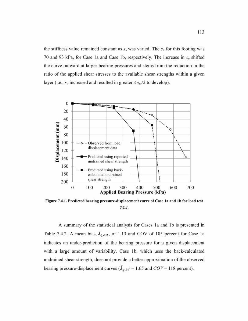
113

the stiffness value remained constant as su was varied. The su for this footing was

70 and 93 kPa, for Case 1a and Case 1b, respectively. The increase in su shifted

the curve outward at larger bearing pressures and stems from the reduction in the

ratio of the applied shear stresses to the available shear strengths within a given

layer (i.e., su increased and resulted in greater Δσvr/2 to develop).

Figure 7.4.1. Predicted bearing pressure-displacement curve of Case 1a and 1b for load test

TS-1.

A summary of the statistical analysis for Cases 1a and 1b is presented in

Table 7.4.2. A mean bias, , , of 1.13 and COV of 105 percent for Case 1a

indicates an under-prediction of the bearing pressure for a given displacement

with a large amount of variability. Case 1b, which uses the back-calculated

undrained shear strength, does not provide a better approximation of the observed

bearing pressure-displacement curves ( , = 1.65 and COV = 118 percent).

0

20

40

60

80

100

120

140

160

180

2000 100 200 300 400 500 600 700

Dis

pla

cem

ent

(mm

)


Observed from loaddisplacement data

Predicted using reportedundrained shear strength

Predicted using back-calculated undrainedshear strength

114

The bias distributions were modeled using normal and lognormal

distributions. The pronounced curvature of the observed distributions indicates

that Case 1a and Case 1b are better modeled as lognormal. By visual inspection of

Figure 7.4.2 and Figure 7.4.3, there is more variability in the q-δ curves for Case

1b that develops from the upper tail of the distribution where bearing pressures

predicted at a given displacement are over-predicted.

Table 7.4.2. Summary statistics of the Duncan-Chang model application to q-δ curves for

Case 1a and 1b.

, ,

Mean COV Mean COV

1.131 105% 1.647 118%

The tendency for the Duncan-Chang model to under-predict the applied

bearing pressure for a given displacement results from the violation of model

validity at higher mobilized shear strengths. As the ratio of the mobilized

undrained shear strength to the ultimate principle stress difference (Δσvr/2su)

approaches unity, the displacements become unreasonable, as discussed in

Section 7.3. This indicates that as shear stresses beneath the foundation develop

the failure criterion the predicted bearing pressures for a given displacement are

less, producing a bias greater than unity.

115

Figure 7.4.2. Distribution of biases for bearing pressure-displacement curves for Case 1a.

Figure 7.4.3. Distribution of biases for bearing pressure-displacement curves for Case 1b.

Bias

Densi

ty

0 2 4 6 8

0.0

0.5

1.0

1.5

2.0

0 2 4 6 80.0

0.2

0.4

0.6

0.8

1.0

Bias

CD

F

Bias

Densi

ty

0 2 4 6 8

0.0

0.5

1.0

1.5

2.0

0 2 4 6 8

0.0

0.2

0.4

0.6

0.8

1.0

Bias

CD

F



116

7.4.2. Back calculation of the Initial Undrained Young’s Modulus (Case 2)

The application of the Duncan-Chang model to a bearing pressure-

displacement curve enables the estimation of an initial Young’s modulus and can

be optimized by minimizing the sum of the square error between the observed and

predicted displacements. Figure 7.4.4 presents an example of a bearing pressure-

displacement curve for footing TS-1 developed from the iterative procedure that

accurately predicts displacements up to bearing pressures of approximately 480

kPa. At this point, the predicted mobilized undrained shear strength becomes

greater than the available undrained shear strength, and the Duncan-Chang model

becomes invalid (i.e. Δσvr/2 > su). The remaining load test database q-δ curves are

presented in Appendix B. The calculation of the initial Young’s modulus was

facilitated by omitting points beyond where the model becomes invalid and

calculated by rearranging Equation (7.5) which is given as:

where Ein is the initial undrained Young’s modulus averaged over a depth Beq.

Biases were calculated using the applied bearing pressure at a given

displacement for the q-δ curves calculated by the Duncan-Chang model using

estimated and back-calculated undrained shear strengths for Case 2a and Case 2b,

respectively. The expression for the bias was defined previously [Equation (7.8)

and Equation (7.9)], and the pertinent soil parameters for the footing load tests are

presented in Table 5.5.1. The accuracy of the Case 2 approach is presented in

Table 7.4.3. A mean bias of 1.11 for Case 2a indicates a slight over-prediction of

1 2

(7.10)

117

the bearing pressure for a given displacement with a large amount of variability

(COV = 105%).

Figure 7.4.4. Back calculation of initial Young's modulus from Duncan-Chang model using

bearing pressure-displacement curves for load test TS-1 (Case 2).

Case 2b was developed using back-calculated undrained shear strength

provides a better approximation of the observed bearing pressure-displacement

curves ( , = 1.00 and COV = 30 percent). This indicates that the application of

the back-calculated undrained shear strength (Case 2b) in the Duncan-Chang

model better fits the curvature of the observed q-δ curves.

Table 7.4.3. Summary of the bias comparisons for Case 2a and Case 2b.

Case 2a Bias, , Case 2b Bias, ,

Mean COV Mean COV

1.114 44% 1.003 30%

0

20

40

60

80

100

120

140

1600 100 200 300 400 500 600 700 800

Dis

pla

cem

ent

(mm

)


Observed loaddisplacement curve

Predicted usingDuncan-Changmodel

118

The statistical comparison of the biases is presented graphically in Figure

7.4.5 and Figure 7.4.6. Normal and lognormal distributions were fitted to the

observed distribution and indicate that the observed distribution is more

lognormal than normal.

Figure 7.4.5. Distribution of biases for bearing pressure-displacement curves based on

estimated su and back-calculated initial Young’s modulus.

It is important to note that the back-calculated initial Young’s modulus is

dependent on the shape of the predicted bearing pressure-displacement curve

which subsequently varies with undrained shear strength. In some cases the

predicted curvature of the bearing pressure-displacement curve was not in

agreement with the observed curvature and in these instances the fitting procedure

Bias

De

nsi

ty

0 1 2 3 4

0.0

0.5

1.0

1.5

2.0

0 1 2 3 4

0.0

0.2

0.4

0.6

0.8

1.0

Bias

CD

F


119

was modified to estimate the initial portion of the q-δ curve. This was done to

focus on the initial stiffness characteristics.

Figure 7.4.6. Distribution of biases for bearing pressure-displacement curves based on back-

calculated su and back-calculated initial Young’s modulus.

Additionally, deviations in the load test data due to other sources of

uncertainty resulted in an increase in the variability in bearing pressure-

displacement prediction as well as the prediction of the initial Young’s modulus.

Nonetheless, the Duncan-Chang model adequately predicts the pre-failure

displacements of the observed bearing pressure-displacement curve and

subsequent initial undrained Young’s modulus.


120

A statistical analysis was conducted to compare the estimated and back-

calculated initial Young’s modulus calculated using the back-calculated undrained

shear strength. The analysis presented herein only presents the results of the back-

calculated initial Young’s modulus using back-calculated undrained shear

strength (Case 2b) because of its ability to predict the mean bearing pressure-

displacement bias ( , = 1.00) with relatively low variability (COV = 30

percent) compared to that predicted using the estimated undrained shear strength.

Computation of the initial undrained Young’s modulus bias is given as:

where Ein,est and Ein,BC are the estimated and back-calculated initial Young’s

moduli, respectively. Table 7.4.4 presents a summary of the analysis and indicates

that the initial undrained Young’s modulus developed using the relationship

proposed by Duncan and Buchignani (1987) under-predicts the actual, or

extrapolated, initial Young’s modulus ( = 2.2) with a significant amount of

variability (COV = 115%). This under-prediction is not surprising, given that the

Duncan-Chang model uses an initial undrained Young’s modulus, typically based

on the first 0.1% axial strain or less. The type or strain level of the Young’s

modulus referenced by Duncan and Buchignani (1987) is not specified but the

relationship was developed from in-situ testing and could potentially represent a

tangent or secant modulus at 50% of peak strength. Thus, the strain levels for the

estimated and back-calculated Young’s modulus may not be similar, which would

explain the large difference.

,

, (7.11)

121

Table 7.4.4. Summary of Case 2 using back-calculated undrained shear strength.

Initial Undrained Young’s Modulus Bias,

Mean COV

2.21 115%

The resulting initial undrained Young’s modulus bias distribution is

plotted in Figure 7.4.7 with fitted normal and lognormal distributions. The normal

distribution does not capture the general trend of the initial undrained Young’s

modulus and is more lognormally distributed. The results of this analysis indicate

that the procedure for estimating the initial Young’s modulus based on Duncan

and Buchignani (1987) is conservative when used in conjunction with the

Duncan-Chang hyperbolic model, predicting larger displacements for a given

pressure then may be observed.

122

Figure 7.4.7 Sample and fitted distributions for the initial Young’s modulus bias.

7.4.3. Elasticity-Based Displacement Prediction (Case 3)

The initial undrained Young’s modulus developed using the relationship

suggested by Duncan and Buchignani (1987) and back-calculated from the

Duncan-Chang model were used to estimate the applied bearing pressure for

displacements of 10, 25, and 50 mm for the footing load tests using the elasticity-

based displacement method (see Chapter 2). This analysis is identified as Case 3

in Table 7.4.1. The elasticity-based bearing pressure was calculated by

rearranging Equation (2.24) to solve for qapp:

1

(7.12)

Bias

Densi

ty

0 2 4 6 8

0.0

0.5

1.0

1.5

2.0

0 2 4 6 8

0.0

0.2

0.4

0.6

0.8

1.0

Bias

CD

F


123

where qeapp is the applied bearing pressure calculated using elasticity-based

methods and all other variables are previously defined. The estimated qeapp was

compared to the observed bearing pressure-displacement curves (Case 3) as

presented in Figure 7.4.8 where applied bearing pressures were linearly

interpolated between provided points. Biases were calculated as:

Figure 7.4.8. Comparison of elasticity-based prediction displacement for load test TS-1.

Case 3 was separated into two subcases: Case 3a uses the estimated initial

Young’s modulus to calculate the required bearing pressure to achieve various

displacements, and Case 3b uses the back-calculated initial undrained Young’s

modulus. A statistical analysis of Case 3 was conducted to determine the

distribution of the elasticity-based bearing pressure biases. Table 7.4.5 provides a

0

10

20

30

40

50

600 200 400 600 800 1000

Dis

pla

cem

ent

(mm

)


Observed load-displacement dataPredicted using EstimatedStiffness ValuesPredicted using BackCalculated Stiffness

(7.13)

124

summary of the comparison. The mean bias for Case 3a at a displacement value

of 10 mm is 0.80, indicating that the estimated initial undrained Young’s modulus

produces a slightly conservative estimate with high variability (COV = 99

percent). Case 3b over-predicts the bearing pressure required to produce 10 mm

of displacement ( = 0.49) with an even higher variability (COV = 109 percent).

The same trend continues for a displacement of 25 mm where the mean biases for

Case 3a and 3b are 0.49 and 0.33, respectively. At a displacement of 50 mm the

mean biases and variabilities of the observed distributions for Case 3a ( = 0.14,

COV = 67 percent) and Case 3b are very similar ( = 0.14, COV = 87 percent)

indicating that at larger displacements, bearing pressures calculated using

estimated initial undrained Young’s modulus are similar to those calculated using

back-calculated initial undrained Young’s modulus. It is important to note that at

higher displacements the number of biases in the comparison reduced as the

applied bearing pressure calculated using the elasticity-based method exceeded

the bearing capacity of the footing (i.e. qeapp > qult).

Table 7.4.5. Statistical summary of the analysis for Case 3.

δ = 10 mm δ = 25 mm δ = 50 mm Mean COV Mean COV Mean COV

Case 3a Biases 0.80 99% 0.49 99% 0.14 67%

Case 3b Biases 0.49 109% 0.33 109% 0.14 87%

Number of points 30 24 11

Normal and lognormal distributions were fit to the observed bias

distributions. Example distributions for a displacement of 10, 25, and 50 mm are

presented in Figure 7.4.9 through Figure 7.4.14. Visual inspection of these figures

125

indicates that the elasticity-based prediction displacements for Case 3 are

generally more lognormally distributed with the exception of the prediction at 50

mm of displacement, which are approximately more normally distributed.

Figure 7.4.9. Distribution of elasticity-based prediction biases for Case 3a at a displacement

of 10 mm.

Bias

De

nsi

ty

0.0 1.0 2.0 3.0

0.0

0.5

1.0

1.5

2.0

2.5

0.0 1.0 2.0 3.0

0.0

0.2

0.4

0.6

0.8

1.0

Bias

CD

F


126

Figure 7.4.10. Distribution of elasticity-based prediction biases calculated for Case 3b at

displacement of 10 mm.


of 25 mm.

Bias

De

nsi

ty

0.0 1.0 2.0 3.0

01

23

4

0.0 1.0 2.0 3.0

0.0

0.2

0.4

0.6

0.8

1.0

Bias

CD

F

Bias

De

nsi

ty

0.0 0.5 1.0 1.5

0.0

0.5

1.0

1.5

2.0

0.0 0.5 1.0 1.5

0.0

0.2

0.4

0.6

0.8

1.0

Bias

CD

F



127




of 50 mm.

Bias

De

nsi

ty

0.0 0.5 1.0 1.5

01

23

0.0 0.5 1.0 1.50

.00

.20

.40

.60

.81

.0

Bias

CD

F

Bias

De

nsi

ty

0.0 0.1 0.2 0.3

02

46

8

0.00 0.10 0.20 0.30

0.0

0.2

0.4

0.6

0.8

1.0

Bias

CD

F



128



7.4.4. Back-calculation of the K-factor (Case 4)

The results from the previous analysis were used to back-calculate the K-

factor that is typically used with elasticity-based methods. To assess the effect of

variations in the initial undrained Young’s modulus and undrained shear strength,

the analysis was separated into two cases: Case 4a compares the effect of

undrained Young’s modulus while holding the undrained shear strength constant

and Case 4b compares the effect of undrained shear strength while holding the

initial Young’s modulus constant. For Case 4a, the K-factor is calculated by

rearranging Equation (2.30) which results in the following relationships:

Bias

De

nsi

ty

0.0 0.1 0.2 0.3 0.4 0.5

02

46

8

0.0 0.1 0.2 0.3 0.4

0.0

0.2

0.4

0.6

0.8

1.0

Bias

CD

F


129

where KBC and KE,est are the elasticity-based K-factors calculated using back-

calculated and estimated initial undrained Young’s modulus, respectively. A

statistical comparison of the accuracy of the K-factor was conducted using the K-

factor bias, λK,E, given by:

For Case 4b, similar expressions for the bias may be developed:

where Ksu,est is the K-factor calculated using the estimated undrained shear

strength. Table 7.4.6 presents a summary of the analyses for Case 4a and 4b. It

indicates that on average, the KE,est ( , = 1.05) is fairly accurate K-factor, with a

very high amount of variability (COV = 81 percent). The statistical results of Case

4b show that Ksu,est over-predicts the actual value ( , = 1.39) by about 40

percent with high variability (COV = 56 percent). The combined K-factor

estimates the general trend in the K-factor incorporating the variability in both the

,

,

(7.14)

,

,

,

(7.15)

,

, (7.16)

,

,

,

(7.17)

,

,

(7.18)

130

initial undrained Young’s modulus and undrained shear strength. It is calculated

using the method discussed in Section 8.3 and indicates that in general the

estimated K-factor under-predicts the actual (extrapolated) K-factor.

The distributions for Case 4a and 4b are presented in Figure 7.4.15 and

Figure 7.4.16 along with fitted normal and lognormal distributions. The figures

indicate that KE,est is more lognormally distributed and the Ksu,est is more normally

distributed.

Table 7.4.6. Summary of the statistical analysis of Case 4a and 4b.

Mean COV Case 4a K-factor bias, , 1.05 81%

Case 4b K-factor bias, , 1.39 56%

Combined K-factor bias, 1.46 98%

Figure 7.4.15. Case 4a K-factor bias distribution with fitted distributions.

Bias

De

nsi

ty

0 1 2 3

0.0

0.2

0.4

0.6

0.8

1.0

0 1 2 3

0.0

0.2

0.4

0.6

0.8

1.0

Bias

CD

F


131

Figure 7.4.16. Case 4b K-factor bias distribution with fitted distributions.

7.5. Summary

This chapter presents the development of the Duncan-Chang model and its

uncertainty in application to footing load tests. The method of estimating stiffness

characteristics proposed by Duncan and Buchignani (1987) was adapted into the

Duncan-Chang model to estimate the accuracy and uncertainty in prediction of

footing q-δ curves for estimated and back-calculated undrained shear strengths.

The rearrangement of the Duncan-Chang model facilitated the back-calculation of

the initial Young’s modulus and was compared to the estimated stiffness to assess

the uncertainty associated with its prediction. To present the uncertainty

associated with elasticity-based displacement, q-δ curves were calculated for a

given displacement and compared to the observed q-δ curves. Additionally,

Bias

De

nsi

ty

0.0 1.0 2.0 3.0

0.0

0.2

0.4

0.6

0.8

1.0

1.2

0.0 1.0 2.0 3.0

0.0

0.2

0.4

0.6

0.8

1.0

Bias

CD

F


132

variations in the back-calculated elasticity-based K-factor were presented. The

conclusions and contributions presented in this chapter include:

1. The Duncan-Chang model can adequately predict the pre-failure

undrained bearing pressure-displacement behavior ( , = 1.13) with

very high variability (COV = 105 percent) using estimated undrained shear

strengths.

2. The use of undrained shear strengths back-calculated from the hyperbolic

model does not appear to improve the prediction of q-δ curves using the

Duncan-Chang model ( , = 1.65, COV = 118 percent).

3. The estimated stiffness relationship proposed by Duncan and Buchignani

(1987) generally under-predicts the initial undrained Young’s modulus at

low strains when used in conjunction with the Duncan-Chang model at

low strains ( = 2.2) with a very significant amount of variability (COV

= 115 percent).

4. The elasticity-based method using the estimated initial undrained Young’s

modulus over-predicts the applied bearing pressure required to produce a

displacement of 10 mm ( = 0.80) with a significant amount of

variability (COV = 99 percent).

5. There is a high amount of variability associated with the prediction of

displacements using the Duncan-Chang and elasticity-based methods.

6. The K-factor from Duncan and Buchignani (1987) generally

underestimates the actual K-factor calculated using the Duncan-Chang

model at low strains ( = 1.49), but is also characterized by a large

amount of uncertainty (COV = 98 percent).

133

Chapter 8: Calibration of Resistance Factors for the Bearing

Capacity Model

8.1. Introduction

Reliability-based design (RBD) is an approach that takes the probabilistic

distributions of the applied loads and compares them to the distribution of

resistances to achieve a certain level of performance quantified by “risk”. The

movement to adopt calibration techniques to assess the uncertainty and reliability

using RBD design specifications by the civil engineering profession, such as the

Load and Resistance Factor Design (LRFD) Bridge Design Specifications

(AASHTO, 2007), has increased the demand to acquire and calibrate observed

data. For the present study, the database presented in Chapter 4 and the analysis

discussed in Chapter 6 were used to develop a relationship between an index of

reliability and resistance factors or partial factors of safety. These were developed

for representative loading conditions accounting for uncertainty in prediction

models and loading uncertainty to assess footing performance based on the

probability of failure. The calibration and development of load and resistance

followed the procedure given by Allen et al. (2005):

1. Develop the limit state equation to be evaluated;

2. Produce statistical characterizations of the data set to be calibrated;

3. Select a target reliability level based on the desired margin of safety; and,

4. Calculate resistance factors using reliability theory and American

Association of State Highway and Transportation Officials (AASHTO)

load factors.

134

8.2. Limit State Design

There are two types of limit state design (LSD) that are generally

considered in the LRFD method: the strength and serviceability limit states. The

strength limit state refers to the structural safety of a system and is considered to

be an ultimate state, implying a collapse of the system when exceeded. For

shallow footings the strength limit state is considered to be bearing capacity. The

serviceability limit state refers to any number of conditions where a certain degree

of performance is targeted under characteristic loading conditions and is typically

defined by limiting settlement of a foundation. Regardless of the limit state

considered, the following equation can be used to represent the limit state design

(Allen, et al., 2005):

∗ ∗ (8.1)

where γi is a load factor applied to a specific loading component, Qni is a specific

nominal load component, ΣγiQni is the total factored load for the load group

applicable to the serviceability limit state being considered, ϕR is the resistance

factor, and Rn is the nominal resistance available.

Load and resistance factors are used to account for the uncertainty

associated with material variability, uncertainty in the magnitude of applied loads,

model prediction uncertainty, and any other sources of uncertainty. Equation (8.1)

is considered to be the design equation but serves as a basis for the creation of a

limit state equation that can be applied in a calibration procedure. The use of trial

geometry with a single load component is typically employed in the calibration

procedure in which rearrangement of Equation (8.1) is given by:

135

∗ ∗ 0 (8.2)

where γQ is a load factor. The limit state equation corresponding to Equation (8.2)

is given by:

0 (8.3)

where g is a random variable representing the safety margin, R is a random

variable representing resistance, and Q is a random variable representing load.

The method of calibration for LRFD defines the realization of the limit state as

the point when the applied load is equal to available resistance, at which point

“failure” will occur (i.e. g < 0). The combination of load and resistance factors

produces a design that has a relatively predictable probability (or risk) of failure.

Load and resistance factors are calculated by rearranging Equation (8.2) and

setting it equal to zero, defining the point at which a limit of failure state occurs in

terms of the minimum required resistance:

∗ (8.4)

The magnitude of load and resistance factors and corresponding margin of

safety, g, are calculated such that the estimated probability of failure, Pf, that Q is

greater than R is reasonably small. The conceptual idea is to separate the load and

resistance distributions far enough apart that the area beneath the overlapping

portion of the distributions, defined as the probability of failure, is acceptable.

This is illustrated in Figure 8.2.1 where the R distributions are presented by two

PDFs sharing a mean value, , but different uncertainties and the Q distribution is

136

presented by a single distribution having a mean value, . The allowable

probability of failure is calculated by developing the PDF of the margin of safety.

The reliability of the system is assessed using the reliability index, β, which is the

number of standard deviations separating the mean margin of safety, , from zero

(Allen, et al., 2005). This is illustrated conceptually in Figure 8.2.2.

When the limit state function is a linear relationship, the variables

representing loads and resistances are normally distributed, and are not correlated,

the reliability index is given by (Allen, et al., 2005):

(8.5)

where σR and σQ are the standard deviations of the resistance, R, and load, Q,

respectively. For lognormal distributions of loads and resistances, the reliability

index may be approximated using:

ln ∗

11

ln 1 ∗ 1 (8.6)

where COVR and COVQ are the coefficient of variations for resistance, R, and

load, Q, respectively. For a normally distributed margin of safety the probability

of failure is given by:

137

1 (8.7)

where Φ returns the probability associated with the reliability index.

Figure 8.2.1. Conceptual illustration of potential probability density functions (PDFs) for

load and resistance factors, from (Stuedlein, 2008).

138

Figure 8.2.2. Conceptual illustration of a combined PDF representing the margin of safety

and the reliability index, adapted from (Stuedlein, 2008).

8.3. Statistical Characterization of Resistance Distribution

The estimation of the margin of safety, g, is defined as the difference

between the available resistance, R, and the applied load, Q. The resistance

distribution was developed from the bearing capacity bias statistics developed in

Section 6.3.1. The distribution of the bias set is re-plotted in Figure 8.3.1 using

the data pairs of standard normal variate and bias values (see Section 6.2). Data

that is normally distributed plots as a linear relationship where lognormal

distributions exhibit pronounced curvature.

A theoretical lognormal distribution was fit to the observed distribution by

minimizing the sum of the square error between the observed and predicted bias

distribution. To capture the lower tail of the observed distribution where biases

are less than unity, or the predicted bearing capacity is greater than that observed,

the lognormal distribution was fit to the lower tail of the observed distribution by

139

omitting portions of the observed distribution during the summation of the

squared errors (Bathurst, et al., 2008). This procedure develops a model that

focuses on the load tests that are essentially non-conservative. The fitted

lognormal distribution, termed as fit-to-tail model, is presented in Figure 8.3.1

and summarized in Table 8.3.1.

Table 8.3.1. Summary of theoretical distribution fitting of the bearing capacity bias

distribution.

Nominal Bearing Capacity Bias

Distribution Mean COV

Normal, λBC 1.30 39%

Lognormal, λBC 1.30 39%

Fit-to-Tail Lognormal, λBC,fit 1.38 49%

The probabilistic input parameters developed from the fit-to-tail model

( , = 1.38 and COV = 49%) presented in Table 8.3.1 were used to develop a

lognormal resistance distribution, Rn; where Rn is given by:

, ∗ (8.8)

140

Figure 8.3.1. CDF of standard normal variate as a function of bearing capacity prediction

biases.

The distribution of the margin of safety was produced by finding the

difference between the combined loading distribution, Qcombined, and the fit-to-tail

bearing resistance distribution, Rn, for a given dead load to live load (DL/LL)

ratio. Determination of the reliability index for a lognormal distribution, β,

required the summation of the occurrences of the margin of safety that were

negative (g < 0), corresponding to the case where the applied bearing pressure

was greater than the available capacity. The probability of failure, pf, was

-2.5

-2.0

-1.5

-1.0

-0.5

0.0

0.5

1.0

1.5

2.0

2.5

0.0 0.5 1.0 1.5 2.0 2.5 3.0

Sta

nd

ard

Nor

mal

Var

iate

Bias

Experimental Bias

Fitted Normal Distribution

Fitted Lognormal Distribution

Fit-to-Tail LognormalDistribution

141

calculated by dividing the number of negative g values by the total number of

random variables; in this study 50,000 random estimates were used. The

reliability index was then calculated using:

(8.9)

where Φ-1 returns the standard normal variate for a given probability based on the

a normal cumulative density function.

The bearing capacity model presented herein should consider the

calculation of the total bias, λfinal, and the total coefficient of variation, COVfinal,

used to combine sources of uncertainty as presented in Equations (6.13) and

(6.14). However, the lack of correlation between the observed and predicted

bearing capacities, as discussed in Section 6.3.1, indicates that no additional

model adjustments are needed if the uncertainty associated with the undrained

shear strength is neglected. It is also important to note that the model is very

accurate for bearing capacity biases that are less than unity and intentionally not

accurate at biases greater than unity. The mean bias for the fit-to-tail bearing

capacity model indicates that the general bearing capacity formula under-predicts

the available (extrapolated) bearing capacity ( , = 1.38) with a significant

amount of variability (COV = 49 percent). If the variability of the undrained shear

strength were incorporated into the model, the uncertainty associated with the fit-

to-tail model would increase significantly, as shown in Table 8.3.2.

142

Table 8.3.2. Final statistics of the adjusted fit-to-tail lognormal bearing capacity model.

, ,

1.38 49% 39%

0% 49%

20% 66%

30% 70%

50% 80%

8.4. Resistance Factor Calibration using the Monte Carlo Approach

For the present study, the Monte Carlo simulation method discussed in

Section 6.3.4 was used to extrapolate the CDF of the bearing capacity prediction

biases based on a distribution fitted to the observed biases discussed in Section

6.3.1. Random values of Q and R with defined statistics and distributions were

used to estimate the distribution of margin of safety, g.

The applied loads considered were assumed to come from lognormal

distributions with COV’s specified using AASHTO load statistics (AASHTO,

2007). The Monte Carlo method generates a specified number of variables, which

are used to simulate independent standard normal variates representative of the

distributions of load, Q, and resistance, R. The random standard normal variates

were generated using Equation (8.9). Where normal random sample generation

was used, the transformation to log-space was performed to develop lognormal

distributions. The resistance and applied load distributions were simulated using

independent data sets of 50,000 random standard normal variates to achieve an

appropriate level of statistical accuracy.

The Monte Carlo simulation requires that probabilistic input parameters be

selected to account for the variability in both load and resistance. In many cases,

the variability in the loading conditions is defined by a governing agency such as

143

the AASHTO. For this study the probabilistic input parameters used to estimate

the loading distribution were selected based on design specifications defined by

AASHTO. The probabilistic parameters are provided in Table 8.4.1.

Table 8.4.1. Summary of AASHTO loading and bias statistics (Paikowsky, et al., 2004).

Load Condition Load Factor Load Bias Load COV

Live γL = 1.75 λQL = 1.15 COVQL = 0.2

Dead γD = 1.25 λQD = 1.05 COVQD = 0.1

The load factor essentially incorporates a factor of safety against

unexpected loading conditions, whereas the load bias accounts for the differences

between the observed and predicted loading conditions. The COV accounts for

model variability. A combined loading factor (Stuedlein, et al., 2012) was

calculated to account for the bias effects associated with the applied loading and

is given by:

, (8.10)

where DL/LL is the ratio of the applied dead load to live load. Independent

lognormal distributions were developed for the applied dead load, QDL, which are

given as:

(8.11)

144

where μln and σln are calculated using AASHTO load and bias factors for the

given loading condition as presented in Section 6.2. A similar approach was taken

for the live load. The individual distributions were combined to create an

averaged distribution that accounts for the biases and variability in live and dead

loading conditions. The calculation of the combined distribution is given as

(Stuedlein, et al., 2012):

1 (8.12)

8.5. Target Reliability Indices and Calculation of Load and Resistance

Factors

Resistance factors are calibrated using a reliability index that corresponds

to a specified probability of failure. Typical design probabilities of failure are 1

and 0.1 percent which correspond to reliability index values of 2.33 and 3.09,

respectively. The process of calculating a reliability index was repeated for

selected DL/LL ratios to estimate the resistance factor, ϕR. The resulting resistance

factors for the fit-to-tail lognormal bearing capacity without considering the

uncertainty in undrained shear strength are presented in Figure 8.5.1 and a DL/LL

equal to 200 was calculated to simulate a zero live load condition.

145

Figure 8.5.1. Resistance factors for calculating bearing capacity without considering

uncertainty in undrained shear strength.

For a project that is to be designed using AASHTO loading statistics, the

acceptable probability of failure is 0.1 percent (β = 3.09) and no defined live load

the resistance factor, ϕR, is given as 0.392. Similarly, if an acceptable probability

of failure is one percent (β = 2.33) a bearing capacity resistance factor of

approximately 0.41 should be used in the design. For example, if the typical

footing discussed in Section 6.3.4 (qult = Rn = 313 kPa) was analyzed using

AASHTO statistics to determine the maximum allowable dead load for a β of

3.09, the combination of resistance factor (ϕR = 0.39) and combined loading factor

(γQ,combined = 1.25) would result in a maximum allowable applied bearing pressure

of 98 kPa (FS = 3.2).

0

0.1

0.2

0.3

0.4

0.5

0.6

0.7

1 2 3 4 5 6 7 8 9 10

Res

ista

nce

Fac

tor,

ϕR

Dead Load/Live Load (DL/LL)

β = 2.33

β = 3.09

DL/LL = 200

DL/LL = 2000.392

0.044

0.5610.045

146

The resistance factors are not very sensitive to DL/LL ratio because the

variability in final bearing capacity model (COV = 63%) is much greater than the

variability in the dead (COVQD = 10 percent) and live loads (COVQL = 20 percent).

Equations for the resistance factors as a function of DL/LL and β are presented in

Figure 8.5.1 for proposed unusual span lengths. Note that the DL/LL should not be

rounded to the nearest 0.05, as this would alter the associated probability of

failure (Phoon & Kulhawy, 1999).

8.6. Summary

The growth in code-based design of structures facilitates the increase of

reliability based design methods for shallow foundations on clay. A bearing

pressure regression model allowed the statistical calibration of a bearing capacity

bias distribution. The incorporation of variability stemming from the regression

model and loading distribution enabled the estimation of resistance factors for

various loading conditions. Contributions and conclusions stemming from this

study presented herein include:

1. A fit-to-tail lognormal bearing capacity model that adequately captures

the lower tail of the observed bearing capacity bias distribution ( ,

= 1.38 and COV = 49%) was produced;

2. The effect of the variability of the undrained shear strength was

presented and quantified based on available case histories;

3. Equations for estimation of LRFD resistance factors for typical design of

bearing capacity using AASHTO load factors were developed for

reliability indices of 2.33 and 3.09:

2.33: 0.561.

3.09: 0.392.

147

Chapter 9: Summary and Conclusions

9.1. Summary

Improvements of the general bearing capacity formula and bearing

pressure-displacement prediction methods of isolated shallow foundations have

been slow in developing. The general bearing capacity formula typically used to

predict the available resistance of a footing assumes perfectly plastic soil

behavior, (i.e., sudden failure will occur when the bearing capacity is exceeded),

which does not incorporate strength mobilization as a load is applied. A

hyperbolic bearing pressure-displacement model was adopted to extrapolate

bearing capacity from case histories presented in the literature. These were

compared to the bearing capacities predicted using the general bearing capacity

formula to assess the uncertainty associated with the use of the formulas.

Prediction of distortion displacements of shallow foundations is primarily

limited to elasticity-based methods, which ignore the nonlinearity of soil. Some

existing methods account for nonlinear soil behavior, but they are too

computationally intensive or require large quantities of high quality testing to

accurately predict displacement. This study aimed to improve bearing pressure-

displacement prediction methods by the application of the Duncan-Chang soil

constitutive model.

A database consisting of footing load tests available in the literature was

used to evaluate existing methods of bearing capacity and displacement. The

research program consisted of soil profile characterizations to produce pertinent

soil parameters and the application of existing and proposed bearing capacity and

bearing pressure-displacement prediction techniques to assess model uncertainty.

The uncertainty associated with bearing pressure-displacement models was

148

presented. A summary of all the analyses conducted in this study is presented in

Table 9.2.1.

9.2. Conclusions

The completed research and findings are summarized for the uncertainty

in bearing capacity prediction, uncertainty in prediction of bearing pressure-

displacements, and proposed model for performance prediction are summarized in

the following sections.

9.2.1. Uncertainty in Bearing Capacity Predictions

1. The hyperbolic model accurately fits q-δ curves produced by footings on

clay with a relatively low amount of uncertainty ( = 1.13, COV = 22

percent);

2. Predicted bearing capacities are considered to be statistically independent

from the actual (extrapolated) bearing capacities (two sided p-value =

0.13);

3. Bearing capacity predicted using the general bearing capacity formula

under-predicts the actual (extrapolated) bearing capacity with a relatively

high amount of uncertainty ( = 1.30, COV = 39 percent);

4. The incorporation of surcharge effects in the general bearing formula may

increase the available bearing capacity by approximately 5 percent and

produce a more accurate prediction ( = 1.37, COV = 38 percent);

5. Model uncertainty greatly increased the variability in bearing capacities

calculated using the general bearing capacity formula and reduced the

effect of variability of undrained shear strength on bearing capacity, and

149

6. The use of su,mob-δ curves predicts the estimated undrained shear strengths

relatively accurately ( = 1.17) on average, although there is also a

relatively high amount of uncertainty (COV = 55 percent). These results

account for the uncertainty associated with applying the bearing capacity

model to develop extrapolate undrained shear strength from su,mob-δ

curves.

9.2.2. Uncertainty in Prediction of Bearing Pressure-Displacement

1. The Duncan-Chang model adequately fits the pre-failure undrained

bearing pressure-displacement behavior;

2. The Duncan-Chang model adequately predicts the pre-failure undrained

bearing pressure-displacement behavior ( , = 1.13) with very high

variability (COV = 105 percent) using estimated undrained shear

strengths;

3. The use of undrained shear strengths back-calculated from the

hyperbolic model greatly improves the fitting of q-δ curves using the

Duncan-Chang model;

4. The estimated stiffness procedure proposed by Duncan and Buchignani

(1987) under-predicts stiffness characteristics when used with the

Duncan-Chang model at low strains, and

5. There is a high amount of variability associated with the prediction of

displacements using the Duncan-Chang and elasticity-based methods.

150

9.2.3. Proposed Model for Bearing Capacity Prediction

1. The statistical fitting of a fit-to-tail lognormal bearing capacity model

that captures the lower tail of the observed bearing capacity bias

distribution ( , = 1.37 and COV = 49 percent) was conducted, and

2. The estimation of bearing capacity resistance factors for typical design

reliability indices of 2.33 and 3.09 were developed using AASHTO load

statistics for footings on clay.

151

Table 9.2.1. Summary of statistical analyses presented in this study.

Symbol Bias description # of Points Mean Bias, COV Distribution*

λBC Nominal bearing capacity with surcharge 30 1.30 39% Lognormal

λoBC Nominal bearing capacity without surcharge 30 1.37 38% Lognormal

λcsu Compounded undrained shear strength 30 1.17 55% Lognormal

λE Initial undrained Young's modulus 30 2.21 115% Lognormal

λeq

Elasticity-based bearing pressure:estimated stiffness

δ = 10 mm 30 0.80 99% Lognormal

δ = 25 mm 24 0.49 99% Lognormal

δ = 50 mm 11 0.14 67% Normal

λeq

Elasticity-based bearing pressure:back-calculated stiffness

δ = 10 mm 30 0.49 109% Normal

δ = 25 mm 24 0.33 109% Lognormal

δ = 50 mm 11 0.14 87% Normal

λK,E Initial undrained Young's modulus K-factor 30 1.05 81% Lognormal

λK,su Undrained shear strength K-factor 30 1.39 56% Normal

λBC,fit Fit-to-tail Lognormal Model 21 1.37 49% Lognormal

*Inferred from PDFs or CDFs

152

Bibliography

AASHTO, 2007. LRFD Bridge Design Specifications. 4th ed. Washington, D.C.: AASHTO.

Allen, T., Nowak, S. and Bathurst, R., 2005. Calibration to Determine Load and Resistance Factors for Geotechnical and Structural Design, Washington, D.C.: Transportation Research Board.

Andersen, K. H. and Stenhamer, P., 1982. Static Plate Loading Tests on Overconsolidated Clay. Journal of the Geotechnical Engineering Division, 108(GT7), pp. 918-934.

Bathurst, R., Allen, T. and Nowak, A., 2008. Calibration concepts for load and resistance factor design (LRFD) of reinforced soil walls. Canadian Goetechnical Journal, Issue 45, pp. 1377-1392.

Bauer, G. E., Shields, D. H. and Scott, J. D., 1976. Predicted and Observed Footing Settlements in a Fissured Clay. Ottawa, Pentech Press, pp. 287-302.

Bergado, D. T., Rantucci, G. and Widodo, S., 1984. Full Scale Load Tests of Granualr Piles and Sand Drains in the Soft Bangkok clay. Paris, Asian Institute of Technology, pp. 111-118.

Bergfelt, A., 1956. Loading Tests on Clay. Geotechnique, pp. 15-31.

Bjerrum, L. and Overland, A., 1957. Foundation Failure of an Oil Tank in Fredrikstad, Norway. London, ASCE, pp. 287-290.

Bond, D., 1961. The Influence of Foundation Size on Settlement. Geotechnique, 11(2), pp. 121-143.

Borowicka, H., 1936. Influence of Rigidity of a Circular Foundation Slab on the Distribution of Pressures Over the Contact Surface. Germany, ASCE, p. 144.

Brand, E. W., Muktabhant, C. and Taechathummarak, A., 1972. Load Tests on Small Foundations in Soft Clay. New York, ASCE, pp. 903-928.

Brown, P., 1969. Numerical Analyses of Uniformly Loaded Circular Rafts on Deep Elastic Foundations. Geotechnique, 19(3), pp. 399-404.

153

Burland, J., 1970. Discussion, Session A. London, British Geotechnical Society, pp. 61-62.

Carrier, D. I. and Christian, J., 1978. Janbu, Bjerrum and Kjaernsli's chart reinterepreted. Canadian Geotechnical Journl, Volume 15, pp. 123-128.

Chen, W. and McCarron, W., 1991. Bearing Capacity of Shallow Foundations. In: H. Fang, ed. Foundation Engineering Handbook. Second ed. New York: Chapman and Hall, pp. 144-165.

Chin, F., 1971. Estimation of the Ultimate Load of Piles from Tests not Carried to Failure. Singapore, University of Singapore, pp. 81-90.

Coduto, D., 2001. Foundation Design: Principals and Practices. 2nd ed. New Jersey: Prentice-Hall Inc..

Consoli, N. C., Schnaid, F. and Milititsky, J., 1998. Interpretation of Plate Load Tests on Residual Soil Site. Journal of Geotechnical and Geoenvironmental Engineering, 124(9), pp. 857-867.

D'Appolonia, D., 1965. Prediction of Stress and Deformation for Undrained Loading Conditions, Cambridge: Massechusetts Institute of Technology.

D'Appolonia, D. and Lambe, T., 1970. Method for Predicting Initial Settlement. Journal of the Soil Mechanics and Foundations Division, Issue SM 2, pp. 523-544.

D'Appolonia, D., Poulos, H. and Ladd, C., 1971. Initial Settlement of Structures on Clay. Journal of the Soil Mechanics and Foundations Division, 97(SM10), pp. 1359-1377.

Das, B., 1999. Shallow Foundations: Bearing Capacity and Settlement. Boca Raton(Florida): CRC Press.

Das, B., 2011. Principles of Foundation Engineering. Seventh ed. Stamford, CT: Global Engineering.

Davis, E. and Poulos, H., 1972. Rate of Settlement under two- and three- dinensional conditions. Geotechnique, 22(1), pp. 95-114.

De Beer, E., 1970. Experimental Determination of the Shape Factor and the Bearing Capacity Factors for Sand. Geotechnique, 20(4), pp. 387-411.

154

Decourt, L., 1992. SPT in non classical material. Belo Horizonte, ASCE, pp. 67-100.

Deshmukh, A. M. and Ganpule, V. T., 1994. Influence of Flexible Mat on Settlements of Marine Clay. College Station, Texas, American Society of Civil Engineers, pp. 887-896.

Djoenaidi, W., 1985. A Compendium of Soil Properties and Correlations, Sydney: University of Sydney.

Duncan, J. and Buchignani, A., 1987. An Engineering Manual for Settlement Studies, Berkeley: Univeristy of California.

Duncan, J., Byrne, P., Womg, K. and Mabry, P., 1980. Strength, Stress-Strain and Bulk Modulus Parameters for Finite Element Analyses of Stresses and Movements in Soil Masses, Berkeley: University of California.

Duncan, J. and Chang, C., 1970. Nonlinear Analysis of Stress and Strain in Soils. Journal of the Soil Mechanics and Foundations Division, 96(SM3), pp. 1629-1653.

Eden, W. and Bozozuk, M., 1967. Earth Pressures on Ottawa Outfall Sewer Tunnel, Ottawa: National Research Council Canada.

Elhakim, A., 2005. Evaluation of Shallow Foundation Displacements using Soil Small-Strain Stiffness, Atlanta: Georgia Institute of Technology.

Elhakim, A. and Mayne, P., 2006. Foundation Load-Displacement Response from Small-Strain Stiffness. Atlanta, ASCE, pp. 1-6.

Elsayed, A., 2008. A New Approach for Non-Linear Load-Settlement Assessment of Shallow, Reno: University of Nevada Reno.

Foott, R. and Ladd, C., 1981. Undrained Settlement of Plastic and Organic Clays. Journal of the Geotechnical Engineering Division, 107(GT8), pp. 1079-1094.

Foye, K., Basu, P. and Prezzi, M., 2008. Immediate Settlement of Shallow Foundations Bearing on Clay. International Journal of Geomechanics, 8(5), pp. 300-310.

Gibson, R., 1967. Some results concerning displacements and stresses in a non-homogeneous elastic half-space. Geotechnique, Volume 17, pp. 58-67.

155

Gildea, P., 1993. Instrumented Footing Load Tests on Soft Sensitive Bothkennar Clay. Ground Engineering, 26(6), pp. 30-38.

Giroud, J.-P., 1972. Settlement of Rectangular Foundation on Soil Layer. Journal of Soil Mechanics and Foundations Division, 98(SM1), pp. 149-154.

Greenwood, D., 1975. Methods of Treatment of Unstable Ground. In: F. Bell, ed. London: Butterworth and Co., pp. 189-209.

Han, J. and Ye, S., 1991. Field tests of soft clay stabilized by stone columns in coastal areas in China. Rotterdam, Netherlands, Balkema Press, pp. 243-248.

Hansen, J., 1963. Discussion on Hyperbolic Stress-Strain Response: Cohesive Soils. Journal of the Soil Mechanics and Foundations Division, 89(SM4), pp. 242-243.

Hansen, J., 1970. A revised and extended formula for bearing capacity. DGI Bulletin, pp. 5-11.

Hight, D., Bond, A. and Legge, J., 1992. Characterization of Bothkennar Clay: an overview. Geotechnique, 42(2), pp. 303-347.

Hight, D. W. et al., 1997. Wave velocity and stiffness measurements of the Crag and Lower London Tertiaries at Sizewell. Geotechnique, 47(3), pp. 451-474.

Hight, D. W. and Higgins, K. G., 1995. An approach to the prediction of ground movements in engineering practice: background and applications. Sappo, Balkem Press, pp. 909-945.

Hirany, A. and Kulhawy, F., 1988. Conduct and Interpretation of Load Tests on Drilled Shaft Foundations, New York: EPRI.

Hoeg, K., Andersland, O. B. and Rolfsen, E. N., 1969. Undrained Behaviour of Quick Clay under Load Tests at Asrum. Geotechnique, 19(1), pp. 101-115.

Holtz, R., 1991. Stress Distribution and Settlement of Shallow Foundations. In: H. Fang, ed. Foundation Engineering Handbook. 2nd ed. New York: Chapman and Hall Inc., pp. 167-222.

Holtz, R., Kovacs, W. and Sheahan, T., 2011. An Introduction To Geotechnical Engineering. 2nd ed. Upper Saddle River(NJ): Pearson Education Inc..

156

Janbu, N., 1963. Soil Compressibility as Determined by Oedometer and Triaxial Tests. Wissbaden, Germany, ASCE, pp. 19-25.

Jardine, R. J., 1993. Bearing Capacity and Load-Displacement Behavior of Rigid Pads on Soft Sensitive Clay. St. Louis, ASCE, pp. 161-167.

Jardine, R. J., Lehane, B. M., Smith, P. R. and Gildea, P. A., 1995. Vertical loading experiments on rigid pad foundations at Bothkennar. Geotechnique, 45(4), pp. 573-597.

Jeon, S. and Kulhawy, F., 2001. Evaluation of Axial Compression Behavior of Micropiles. Blacksburg, Virginia, ASCE, pp. 460-471.

Johnson, L. D., 1989. Design and Construction of Mat Foundations, Vicksburg: U.S. Army.

Jones, A., Kramer, S. and Arduino, P., 2002. Estimation of Uncertainty in Geotechincal Properties for Performanced-Based Earthquake Engineering, s.l.: Pacific Earthquake Engineering Research Center.

Kondner, R., 1963. Hyperbolic Stress-Strain Response: Cohesive Soils. Journal of the Soil Mechanics and Foundations Division, February, 89(SM1), pp. 115-144.

Kriegel, H. J. and Weisner, H. H., 1973. Problems of stress-strain conditions in subsoil. Moscow, ASCE, pp. 133-141.

Kulhawy, F., 1992. On Evaluation of Static Soil Properties. Stability and performance of slopes and Embankments II, Issue GSP 31, pp. 95-115.

Kulhawy, F. and Mayne, P., 1990. Manual on Estimating Soil Properties for Foundation Design, Palo Alto: Electric Power Research Institute.

Kulhawy, F. and Phoon, K., 2006. Some Critical Issues in Geo-RBD Calibrations for Foundations. Geotechnical Engineering inthe Information Technology Age, p. 6.

Ladd, C. C. and Foot, R., 1974. New Design Procedure for Stability of soft clays. Journal of the Geotechnical Engineering Division, 100(GT 7), pp. 763-786.

Ladd, C. et al., 1977. Stress-Deformation and Strength Characteristics. Tokyo, ASCE, pp. 421-494.

157

Larsson, R., 1980. Undrained shear strength in stability calculation of embankments and foundations on soft clays. Canadian Geotechnical Journal, Volume 17, pp. 591-602.

Lehane, B. M., 2003. Vertically loaded shallow foundation on soft clayey silt. ICE - Geotechnical Engineering, 156(1), pp. 17-26.

Lehane, B. M. and Jardine, R. J., 2003. Effects of long-term pre-loading on the performance of a footing on clay. Geotechnique, 53(8), pp. 689-695.

Marsland, A. and Powell, J. J. M., 1980. Cyclic loading tests on 865 mm diameter plates of a stiff clay till. Swansea, Balkema Press, pp. 837-847.

Mayne, P. and Poulos, H., 1999. Approximate Displacement Influence Factors for Elastic Shallow Foundations. Journal of Geotechnical and Geoenvironmental, 125(6), pp. 453-460.

Milovic, D., 1965. Comparison between the calculated and experimental values of the ultimate bearing capacity. Serbia, ASCE, pp. 142-144.

Mitchell, K. and Soga, K., 2005. Fundamentals of Soil Behavior. 3 ed. Hoboken: John Wiley and Sons.

Mitchell, R. J., Sangrey, D. A. and Webb, G. S., 1972. Foundations in the crust of sensitive clay deposits. Ottawa, ASCE, pp. 1051-1072.

Moh, Z., Nelson, J. and Brand, E., 1969. Strength and Deformation Behaviour of Bangkok Clay. Bangkok, ASCE, pp. 287-295.

Newton, V. C., 1975. Ultimate Bearing Capacity of Shallow Footings on Plastic Silt, Corvallis: Oregon State University.

Nordlund, R. L. and Deere, D. U., 1970. Collapse of Fargo Grain Elevator. Journal of the Soil Mechanics and Foundations Division, 96(SM2), pp. 585-607.

Osman, A. and Bolton, M., 2004. A New Approach to the Estimation of Undrained Settlement of Shallow Foundations on Soft Clay. Engineering Practice and Performance of Soft Deposits, pp. 93-98.

158

Osman, A. and Bolton, M., 2005. Simple plasticity-based prediction of the undrained settlement of shallow circular foundations on clay. Geotechnique, 55(6), pp. 435-447.

Osman, A., White, D., Britto, A. and Bolton, M., 2007. Simple Prediction of the Undrained Displacement of a Circular Surface Foundation on Non-Linear Soil. Geotechnique, 57(9), pp. 729-737.

Paikowsky, S. et al., 2004. Load and Resistance Factor Design (LRFD) for Deep Foundations, Washington, D.C.: Transportation Research Board.

Paikowsky, S. and Tolosko, T., 1999. Extrapolation of Pile Capacity From Non-Failed Load Tests, McLean: FHWA.

Perloff, W. and Baron, W., 1976. Soil Mechanics: Principals and Applications. First ed. New York: Ronald Press Company.

Phoon, K. and Kulhawy, K. F., 1999. Characterization of geotechnical variability. Canadian Geotechnical Journal, Issue 36, pp. 6112-624.

Pile, K., 1975. Correlation Between Actual and Predicted Settlements for a Large Test Footing. Sydney, Institution of Engineers.

Puzrin, A. and Burland, J., 1996. A Logarithmic stress-strain function for rocks and soils. Geotechnique, 46(1), pp. 157-164.

Reese, L., Isenhower, W. and Wang, S., 2006. Analysis and Design of Shallow and Deep Foundations. Hoboken, New Jersey: John Wiley and Sons.

Richardson, A. M. and Whitman, W. V., 1963. Effect of strain-rate upon undrained shear resistance of a saturated remoulded fat clay. Geotechnique, 13(4), pp. 310-324.

Rilling, B. and Smoltczyk, U., 1994. Ultimate Bearing Capacity Tests of Shallow Foundations on Compacted Cohesive Soils. New Delhi, Balkem Press, pp. 563-566.

Roberts, L. and Misra, A., 2010. LRFD of Shallow Foundations at the Service Limit State. Georisk, 4(1), pp. 13-21.

Saye, S. R., 1984. Settlement of Three Grain Tanks on Alluvial Soils Exhibiting Dessication Profiles. St. Louis, Missouri, ASCE, pp. 1033-1039.

159

Schnaid, F., Wood, W. R., Smith, A. K. C. and Jubb, P., 1993. An investigation of bearing capacity and settlements of soft clat deposits at Shellhaven. Oxford, ASCE, pp. 609-627.

Sheahan, T., Ladd, C. and Germaine, J., 1996. Rate-Dependent Undrained Shear Behavior of Saturated Clay. Journal of Geotechnical Engineering, 122(2), pp. 99-108.

Shields, D. and Bauer, G. E., 1975. Determination of the Modulus of Deformation of a Sensitive Clay using Laboratory and In-Situ Tests. Raleigh, North Carolina, ASCE, pp. 395-421.

Skempton, A., 1951. The Bearing Capacity of Clays. London, Building Research Congress, pp. 180-189.

Skempton, A. and Bjerrum, L., 1957. A Contribution to the Settlement Analysis of Foundations on Clay. Geotechnique, 7(4), pp. 168-178.

Stas, C. and Kulhawy, F., 1984. Critical Evaluation of Design Methods for Foundations Under Axial Uplift and Compression Loading, Palo Alto: Electric Power Research Institute.

Stuedlein, A., 2008. Bearing Capacity and Displacement of Spread Footings on Aggregate Pier Reinforced Clay, Seattle: University of Washington.

Stuedlein, A., 2010. Oregon State University CE 571 Course Notes. Corvallis: Oregon State University.

Stuedlein, A., Neely, W. and Gurtowkski, T., 2012. Reliability-Based Design of Augered Cast-in-Place Piles in Granular Soils. Journal of Geotechnical and Geoenvironmental Engineering, 138(6), p. 23.

Stuedlein, A. W. and Holtz, R. D., 2010. Undrained Displacement Behavior of Spread Footings in Clay. s.l., s.n., pp. 653-669.

Tand, K. and Funegard, E. B. J., 1986. Bearing Capacity of Footings on Clay. Alvin, ASCE, pp. 1017-33.

Terzaghi, K., 1943. Theoretical Soil Mechanics. s.l.:John Wiley and Sons.

Terzaghi, K., Peck, R. and Mesri, G., 1996. Soil Mechanics In Engineering Practice. 3rd ed. New York: John Wiley and Sons.

160

Thamm, B. R., 1976. On Load Tests in Soft Clay. Numerical Methods in Geomechanics, Volume 1, pp. 557-566.

Uzielli, M. and Mayne, P., 2011. Serviceability limit state CPT-based design for vertically loaded shallow foundations on sand. Geomechanics and Geoengineering: An international journal, 6(2), pp. 91-107.

Vesic, A., 1973. Analysis of Ultimate Loads of Shallow Foundations. Journal of the Soil Mechanics and Foundations Division, 99(1), pp. 45-73.

Viggiani, G. and Atkinson, J., 1995. Stiffness of Fine-Grained Soil at Very Small Strains. Geotechnique, 45(2), pp. 249-265.

Vucetic, M., 1994. Cyclic Threshold Shear Strain in Soils. Journal of Geotechnical Engineering, 120(12), pp. 2208-2228.

Ward, W., Marsland, A. and Samuels, S., 1965. Properties of the London Clay at the Ashford Common Shaft: In-situ and Undrained Strength Tests. Geotechnique, 15(4), pp. 321-344.

Wood, D., 1983. Index Properties and Critical State Soil Mechanics. Bangkok, ASCE, pp. 301-309.

161

162

Appendix A: Soil Profile Database

163

Case History: Bangkok, Thailand - 1972 (Brand, et al., 1972)

Figure A-1. Undrained shear strength profile for BB load tests in Bangkok, Thailand

(Brand, et al., 1972).

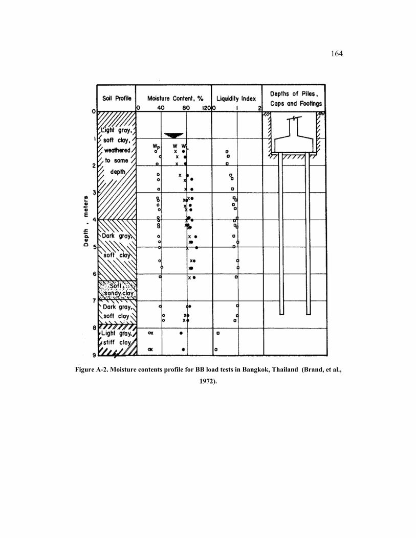
164

Figure A-2. Moisture contents profile for BB load tests in Bangkok, Thailand (Brand, et al.,

1972).

165

Figure A-3. Vertical effect stress, preconsolidation stress and OCR profiles for BB load tests

in Bangkok, Thailand (Moh, et al., 1969).

166

Case History: Corvallis, Oregon, U.S.A. - 1975 (Newton, 1975)

Figure A-4. Moisture contents profile for ON load tests in Corvallis, Oregon (Newton, 1975).

167

Case History: Ottawa, Canada - 1976 (Bauer, et al., 1976)

Figure A-5. Moisture contents, undrained shear strength and vertical stress profile for OB load tests in Ottawa, Canada (Bauer, et al.,

1976).

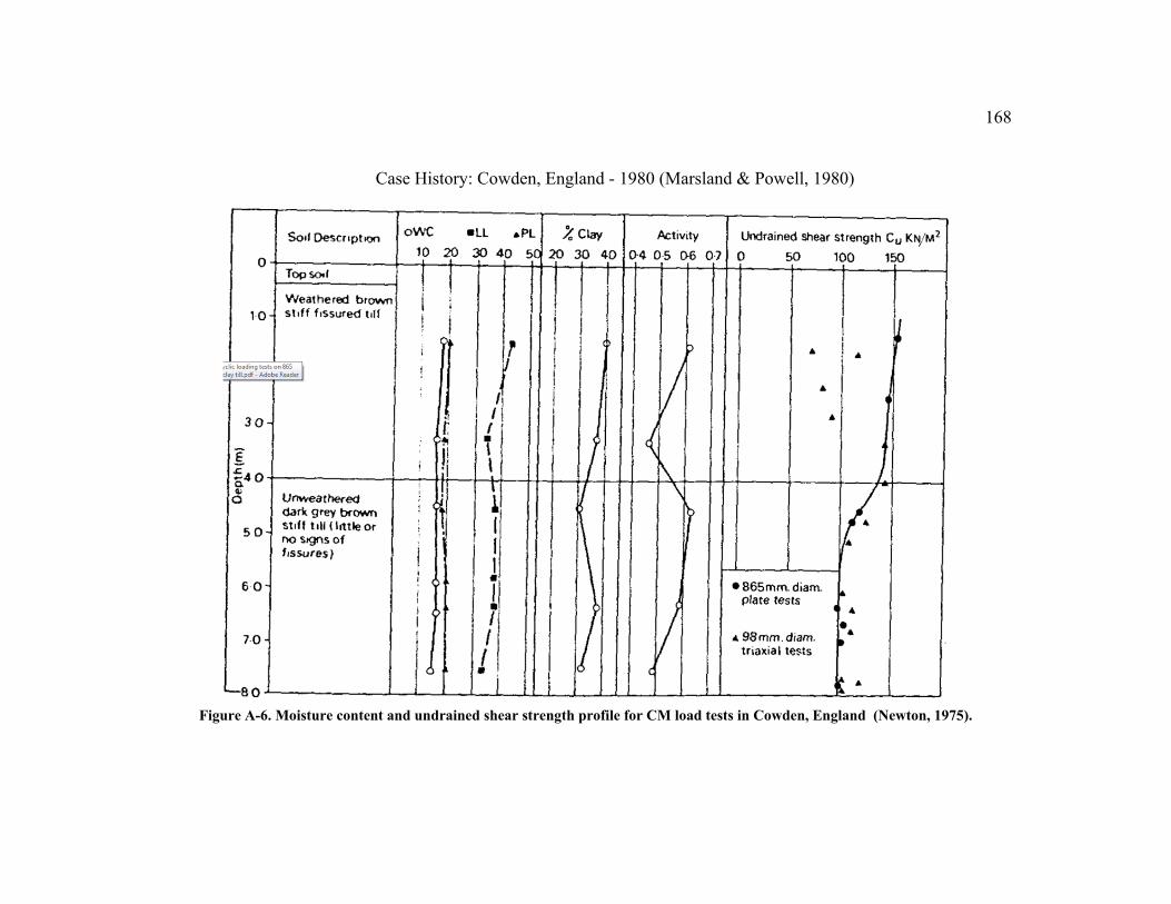
168

Case History: Cowden, England - 1980 (Marsland & Powell, 1980)

Figure A-6. Moisture content and undrained shear strength profile for CM load tests in Cowden, England (Newton, 1975).

169

Case History: Haga, Norway - 1982 (Andersen & Stenhamer, 1982)

Figure A-7. Moisture contents and undrained shear strength profile for HA load tests in Haga, Norway (Andersen & Stenhamer,

1982).

170

Figure A-8. OCR profile for HA load tests in Haga, Norway (Andersen & Stenhamer, 1982).

171

Case History: Bangkok, Thailand - 1984 (Bergado, et al., 1984)

Figure A-9. OCR profile for RB load tests in Bangkok, Thailand (Bergado, et al., 1984).

172

Figure A-10. Vertical and preconsolidation stress profile for RB load tests in Bangkok,

Thailand Invalid source specified..

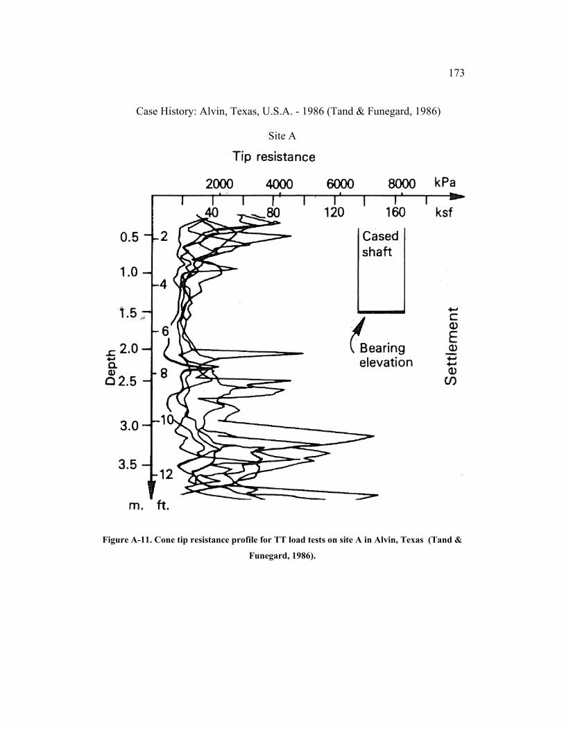
173

Case History: Alvin, Texas, U.S.A. - 1986 (Tand & Funegard, 1986)

Site A

Figure A-11. Cone tip resistance profile for TT load tests on site A in Alvin, Texas (Tand &

Funegard, 1986).

174

Figure A-12. Moisture content, undrained shear strength and pressuremeter profiles for TT load tests on site A in Alvin, Texas (Tand

& Funegard, 1986)

175

Site B

Figure A-13. Cone tip resistance profile for TT load tests on site B in Alvin, Texas (Tand &

Funegard, 1986).

176

Figure A-14. Moisture content, undrained shear strength and pressuremeter profiles for TT load tests on site B in Alvin, Texas (Tand

& Funegard, 1986)

177

Site C

Figure A-15. Cone tip resistance profile for TT load tests on site C in Alvin, Texas (Tand &

Funegard, 1986).

178

Figure A-16. Moisture content, undrained shear strength and pressuremeter profiles for TT load tests on site C in Alvin, Texas (Tand

& Funegard, 1986)

179

Case History: Bothkennar, Scotland - 1993 (Jardine, 1993)

Figure A-17. Undrained shear strength profile for TT load tests on site C in Bothkennar,

Scotland (Tand & Funegard, 1986).

180

Figure A-18. Moisture content profiles for BH load test in Bothkennar, Scotland (Hight, et al., 1992).

181

Figure A-19. Vertical, preconsolidation and OCR profiles for BH load test in Bothkennar, Scotland (Hight, et al., 1992).

182

Case History: Belfast, Ireland - 2003 (Lehane, 2003)

Figure A-20. Moisture content profiles for BL load test in Belfast, Ireland (Lehane, 2003).

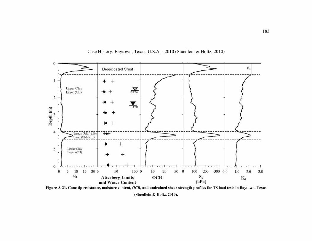
183

Case History: Baytown, Texas, U.S.A. - 2010 (Stuedlein & Holtz, 2010)

Figure A-21. Cone tip resistance, moisture content, OCR, and undrained shear strength profiles for TS load tests in Baytown, Texas

(Stuedlein & Holtz, 2010).

184

Appendix B: Bearing Pressure-Displacement and Transformed

Curves

Appendix Notation:

Notation Definition suest Estimated undrained shear strength suBC Extrapolated undrained shear strength EBC Initial undrained Young's modulus back-calculated using

Duncan-Chang model Eest Estimated initial undrained Young's modulus D-C Duncan-Chang model

185

Figure B-1. Bearing pressure-displacement and transformed hyperbolic curves for load test

BB-1 (Brand, et al., 1972).

0

5

10

15

20

25

30

35

40

45

50

0 50 100 150 200 250 300 350

Dis

pla

cem

ent

(mm

)Applied Bearing Pressure (kPa)

Load Test BB-1

Observed from load test

Hyperbolic prediction

D-C with suest and Eest

D-C with suest and EBC

D-C with suBC and Eest

D-C with suBC and EBC

0.00000

0.00005

0.00010

0.00015

0.00020

0.00025

0.00030

0.00035

0.00 0.01 0.02 0.03 0.04 0.05 0.06

Nor

mal

ized

psu

edo-

stra

in (δ/

B/q

app)

Normalized displacement (δ/B)

Load Test BB-1

Transformed curve

Linear fit

186



0

5

10

15

20

25

30

35

40

0 50 100 150 200 250 300 350

Dis

pla

cem

ent

(mm


Load Test BB-2

Observed from load testHyperbolic predictionD-C with suest and EestD-C with suest and EBCD-C with suBC and EestD-C with suBC and EBC

0.00000

0.00005

0.00010

0.00015

0.00020

0.00025

0.00 0.01 0.02 0.03 0.04 0.05

Nor

mal

ized

psu

edo-

stra

in (δ/

B/q

app)


Load Test BB-2

Transformed curve

Linear fit

187



0

5

10

15

20

25

30

35

40

0 50 100 150 200 250 300 350

Dis

pla

cem

ent

(mm


Load Test BB-3


0.00000

0.00005

0.00010

0.00015

0.00020

0.00025

0.00030

0.00 0.01 0.02 0.03 0.04 0.05 0.06

Nor

mal

ized

psu

edo-

stra

in (δ/

B/q

app)


Load Test BB-3

Transformed curve

Linear fit

188



0

5

10

15

20

25

30

35

40

0 50 100 150 200 250 300 350

Dis

pla

cem

ent

(mm


Load Test BB-4





0.00000

0.00005

0.00010

0.00015

0.00020

0.00025

0.00030

0.00 0.01 0.02 0.03 0.04 0.05 0.06

Nor

mal

ized

psu

edo-

stra

in (δ/

B/q

app)


Load Test BB-4

Transformed curve

Linear fit

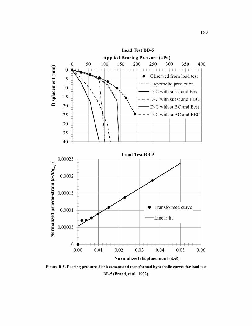
189



0

5

10

15

20

25

30

35

40

0 50 100 150 200 250 300 350 400

Dis

pla

cem

ent

(mm


Load Test BB-5







0

0.00005

0.0001

0.00015

0.0002

0.00025

0.00 0.01 0.02 0.03 0.04 0.05 0.06

Nor

mal

ized

psu

edo-

stra

in (δ/

B/q

app)


Load Test BB-5

Transformed curve

Linear fit

190


GG-1 (Greenwood, 1975).

0

5

10

15

20

25

30

35

40

0 50 100 150 200 250 300

Dis

pla

cem

ent

(mm


Load Test GG-1


0

0.00005

0.0001

0.00015

0.0002

0.00025

0.0003

0.00035

0.0004

0.00 0.02 0.04 0.06 0.08 0.10 0.12

Nor

mal

ized

psu

edo-

stra

in (δ/

B/q

app)


Load Test GG-1

Transformed curve

Linear fit

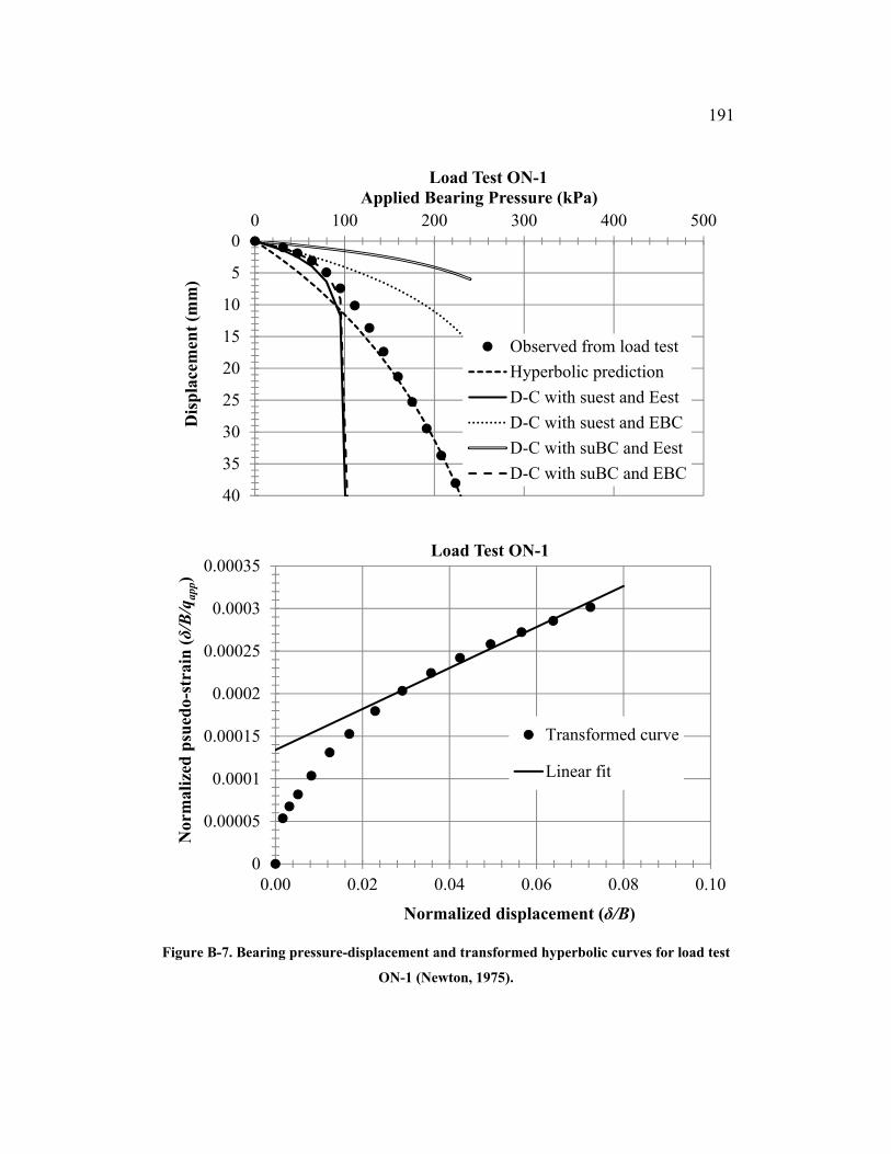
191


ON-1 (Newton, 1975).

0

5

10

15

20

25

30

35

40

0 100 200 300 400 500

Dis

pla

cem

ent

(mm


Load Test ON-1







0

0.00005

0.0001

0.00015

0.0002

0.00025

0.0003

0.00035

0.00 0.02 0.04 0.06 0.08 0.10

Nor

mal

ized

psu

edo-

stra

in (δ/

B/q

app)


Load Test ON-1

Transformed curve

Linear fit

192



0

5

10

15

20

25

30

35

40

0 50 100 150 200

Dis

pla

cem

ent

(mm


Load Test ON-2


0

0.00005

0.0001

0.00015

0.0002

0.00025

0.0003

0.00035

0.0004

0.00045

0.0005

0.00 0.02 0.04 0.06 0.08 0.10

Nor

mal

ized

psu

edo-

stra

in (δ/

B/q

app)


Load Test ON-2

Transformed curve

Linear fit

193



0

5

10

15

20

25

30

35

40

0 50 100 150 200 250

Dis

pla

cem

ent

(mm


Load Test ON-3


0

0.00002

0.00004

0.00006

0.00008

0.0001

0.00012

0.00014

0.00016

0.00018

0.0002

0.00 0.01 0.02 0.03 0.04 0.05

Nor

mal

ized

psu

edo-

stra

in (δ/

B/q

app)


Load Test ON-3

Transformed curve

Linear fit

194


OB-1 (Bauer, et al., 1976).

0

20

40

60

80

100

120

140

160

180

200

0 100 200 300 400 500

Dis

pla

cem

ent

(mm


Load Test OB-1


0

0.0001

0.0002

0.0003

0.0004

0.0005

0.0006

0.0007

0.0008

0.00 0.05 0.10 0.15 0.20 0.25 0.30 0.35

Nor

mal

ized

psu

edo-

stra

in (δ/

B/q

app)


Load Test OB-1

Transformed curve

Linear fit

195


OB-2 (Bauer, et al., 1976).

0

10

20

30

40

50

60

70

80

90

0 100 200 300 400

Dis

pla

cem

ent

(mm


Load Test OB-2


0

0.00005

0.0001

0.00015

0.0002

0.00025

0.00 0.01 0.02 0.03 0.04 0.05 0.06 0.07

Nor

mal

ized

psu

edo-

stra

in (δ/

B/q

app)


Load Test OB-2

Transformed curve

Linear fit

196


CM-1 (Marsland & Powell, 1980).

0

2

4

6

8

10

12

14

16

18

20

0 100 200 300 400 500

Dis

pla

cem

ent

(mm


Load Test CM-1


0

0.00002

0.00004

0.00006

0.00008

0.0001

0.00012

0.00 0.01 0.02 0.03 0.04 0.05 0.06

Nor

mal

ized

psu

edo-

stra

in (δ/

B/q

app)


Load Test CM-1

Transformed curve

Linear fit

197


HA-1 (Andersen & Stenhamer, 1982).

0

10

20

30

40

50

60

70

0 100 200 300 400 500 600 700 800D

isp

lace

men

t (m

m)

Applied Bearing Pressure (kPa)Load Test HA-1


0

0.00002

0.00004

0.00006

0.00008

0.0001

0.00012

0.00014

0.00016

0.00018

0.00 0.01 0.02 0.03 0.04 0.05 0.06

Nor

mal

ized

psu

edo-

stra

in (δ/

B/q

app)


Load Test HA-1

Transformed curve

Linear fit

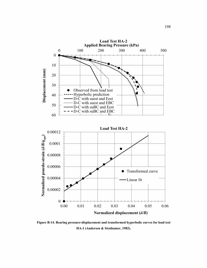
198


HA-1 (Andersen & Stenhamer, 1982).

0

10

20

30

40

50

60

0 100 200 300 400 500

Dis

pla

cem

ent

(mm


Load Test HA-2


0

0.00002

0.00004

0.00006

0.00008

0.0001

0.00012

0.00 0.01 0.02 0.03 0.04 0.05 0.06

Nor

mal

ized

psu

edo-

stra

in (δ/

B/q

app)


Load Test HA-2

Transformed curve

Linear fit

199


RB-1 (Bergado, et al., 1984).

0

2

4

6

8

10

12

14

16

18

20

0 50 100 150

Dis

pla

cem

ent

(mm


Load Test RB-1


0.00000

0.00005

0.00010

0.00015

0.00020

0.00025

0.00030

0.00035

0.00040

0.00045

0.00050

0.00 0.01 0.02 0.03 0.04 0.05 0.06 0.07

Nor

mal

ized

psu

edo-

stra

in (δ/

B/q

app)


Load Test RB-1

Transformed curve

Linear fit

200


TT-1 (Tand & Funegard, 1986).

0

10

20

30

40

50

60

70

80

90

100

0 100 200 300 400 500 600

Dis

pla

cem

ent

(mm


Load Test TT-1


0.00000

0.00002

0.00004

0.00006

0.00008

0.00010

0.00012

0.00014

0.00016

0.00018

0.00020

0.00 0.02 0.04 0.06 0.08 0.10

Nor

mal

ized

psu

edo-

stra

in (δ/

B/q

app)


Load Test TT-1

Transformed curve

Linear fit

201



0

10

20

30

40

50

60

70

0 100 200 300 400 500

Dis

pla

cem

ent

(mm


Load Test TT-2


0.00000

0.00002

0.00004

0.00006

0.00008

0.00010

0.00012

0.00014

0.00016

0.00018

0.00020

0.00 0.02 0.04 0.06 0.08 0.10

Nor

mal

ized

psu

edo-

stra

in (δ/

B/q

app)


Load Test TT-2

Transformed curve

Linear fit

202



0

10

20

30

40

50

60

70

0 100 200 300 400 500 600

Dis

pla

cem

ent

(mm


Load Test TT-3


0.00000

0.00002

0.00004

0.00006

0.00008

0.00010

0.00012

0.00014

0.00016

0.00018

0.00020

0.00 0.02 0.04 0.06 0.08 0.10 0.12

Nor

mal

ized

psu

edo-

stra

in (δ/

B/q

app)


Load Test TT-3

Transformed curve

Linear fit

203



0

10

20

30

40

50

60

70

80

90

100

0 50 100 150 200 250 300

Dis

pla

cem

ent

(mm


Load Test TT-4


0.00000

0.00010

0.00020

0.00030

0.00040

0.00050

0.00060

0.00 0.02 0.04 0.06 0.08 0.10 0.12 0.14 0.16

Nor

mal

ized

psu

edo-

stra

in (δ/

B/q

app)


Load Test TT-4

Transformed curve

Linear fit

204



0

5

10

15

20

25

30

35

40

0 50 100 150 200

Dis

pla

cem

ent

(mm


Load Test TT-5


0.00000

0.00005

0.00010

0.00015

0.00020

0.00025

0.00030

0.00035

0.00 0.01 0.02 0.03 0.04 0.05 0.06

Nor

mal

ized

psu

edo-

stra

in (δ/

B/q

app)


Load Test TT-5

Transformed curve

Linear fit

205



0

5

10

15

20

25

30

35

40

0 200 400 600 800 1000

Dis

pla

cem

ent

(mm


Load Test TT-6


0.00000

0.00002

0.00004

0.00006

0.00008

0.00010

0.00012

0.00 0.01 0.02 0.03 0.04 0.05 0.06 0.07

Nor

mal

ized

psu

edo-

stra

in (δ/

B/q

app)


Load Test TT-6

Transformed curve

Linear fit

206



0

5

10

15

20

25

30

35

40

45

50

0 200 400 600 800

Dis

pla

cem

ent

(mm


Load Test TT-7


0.00000

0.00001

0.00002

0.00003

0.00004

0.00005

0.00006

0.00007

0.00008

0.00009

0.00010

0.00 0.01 0.02 0.03 0.04 0.05 0.06 0.07

Nor

mal

ized

psu

edo-

stra

in (δ/

B/q

app)


Load Test TT-7

Transformed curve

Linear fit

207



0

10

20

30

40

50

60

70

80

0 200 400 600 800

Dis

pla

cem

ent

(mm


Load Test TT-8


0.00000

0.00002

0.00004

0.00006

0.00008

0.00010

0.00012

0.00014

0.00016

0.00 0.02 0.04 0.06 0.08 0.10

Nor

mal

ized

psu

edo-

stra

in (δ/

B/q

app)


Load Test TT-8

Transformed curve

Linear fit

208


BH-1 (Jardine, 1993).

0

20

40

60

80

100

120

140

160

180

200

0 25 50 75 100 125 150

Dis

pla

cem

ent

(mm


Load Test BH-1


0.00000

0.00010

0.00020

0.00030

0.00040

0.00050

0.00060

0.00 0.01 0.02 0.03 0.04 0.05 0.06 0.07 0.08

Nor

mal

ized

psu

edo-

stra

in (δ/

B/q

app)


Load Test BH-1

Transformed curve

Linear fit

209


BD-1 (Deshmukh & Ganpule, 1994).

0

5

10

15

20

25

30

35

40

0 50 100 150 200 250 300 350

Dis

pla

cem

ent

(mm


Load Test BD-1


0.00000

0.00005

0.00010

0.00015

0.00020

0.00025

0.00 0.01 0.02 0.03 0.04 0.05 0.06

Nor

mal

ized

psu

edo-

stra

in (δ/

B/q

app)


Load Test BD-1

Transformed curve

Linear fit

210


BD-1 (Deshmukh & Ganpule, 1994).

0

5

10

15

20

25

30

35

40

0 100 200 300 400

Dis

pla

cem

ent

(mm


Load Test BD-2


0.00000

0.00005

0.00010

0.00015

0.00020

0.00025

0.00 0.01 0.02 0.03 0.04 0.05 0.06

Nor

mal

ized

psu

edo-

stra

in (δ/

B/q

app)


Load Test BD-2

Transformed curve

Linear fit

211


BL-1 (Lehane, 2003).

0

20

40

60

80

100

120

0 20 40 60 80 100 120

Dis

pla

cem

ent

(mm


Load Test BL-1


0.00000

0.00010

0.00020

0.00030

0.00040

0.00050

0.00060

0.00 0.01 0.02 0.03 0.04 0.05 0.06

Nor

mal

ized

psu

edo-

stra

in (δ/

B/q

app)


Load Test BL-1

Transformed curve

Linear fit

212


TS-1 (Stuedlein & Holtz, 2010).

0

20

40

60

80

100

120

140

160

180

200

0 200 400 600 800

Dis

pla

cem

ent

(mm


Load Test TS-1


0.00000

0.00005

0.00010

0.00015

0.00020

0.00025

0.00030

0.00035

0.00 0.05 0.10 0.15 0.20 0.25

Nor

mal

ized

psu

edo-

stra

in (δ/

B/q

app)


Load Test TS-1

Transformed curve

Linear fit

213



0

20

40

60

80

100

120

140

160

180

200

0 200 400 600 800

Dis

pla

cem

ent

(mm


Load Test TS-2


0.00000

0.00005

0.00010

0.00015

0.00020

0.00025

0.00030

0.00035

0.00 0.05 0.10 0.15 0.20 0.25

Nor

mal

ized

psu

edo-

stra

in (δ/

B/q

app)


Load Test TS-2

Transformed curve

Linear fit

214



0

20

40

60

80

100

120

140

160

180

200

0 100 200 300 400 500

Dis

pla

cem

ent

(mm


Load Test TS-3


0.00000

0.00002

0.00004

0.00006

0.00008

0.00010

0.00012

0.00014

0.00 0.01 0.02 0.03 0.04 0.05 0.06

Nor

mal

ized

psu

edo-

stra

in (δ/

B/q

app)


Load Test TS-3

Transformed curve

Linear fit

Date post:	09-Feb-2022
Category:	Documents
Upload:	others
View:	1 times
Download:	0 times

View/Open - Oregon State University

Documents