Virtual certification of acoustic performance for freight ... · Virtual certification of acoustic...

EC Contract No. FP7 - 284877

Collaborative project

Virtual certification of acoustic performance for f reight and passenger trains

D3.9 – Source model for pantograph and bogie aerody namic noise for inclusion in the global simulation model

Due date of deliverable: 31/12/2012

Actual submission date: 04/02/2013

Leader of this Deliverable: Eduardo Latorre Iglesias and David Thompson, ISVR

Reviewed: Y

Document status

Revision Date Description

0 10/12/2012 Draft sent to WP3.5 partners for comment

1 11/01/2013 Uploaded to cooperation tool for final review

2 01/02/2013 Including comments from ATSA and quality review

3 04/02/2013 Including list of figures and tables

4 04/02/2013 Final version after TMT approval

Project co-funded by the European Commission within the Seven Framework Programme (2007-2013)

Dissemination Level PU Public X PP Restricted to other programme participants (including the Commission Services)

RE Restricted to a group specified by the consortium (including the Commission Services)

CO Confidential, only for members of the consortium (including the Commission Services)

Start date of project: 01/10/2011 Duration: 36 months


ACT-T3_5- D-ISV-004-04 Page 2 of 47 04/02/2013

EXECUTIVE SUMMARY

A component-based semi-empirical model is proposed as a prediction model for the aerodynamic noise radiated by generic pantographs and bogies of a high-speed train. Two different component-based models, which have been successfully applied to aerodynamic noise from airplane landing gears by Guo and by Smith, have been used as the starting point. During this work, Guo’s model has been adapted for the case of the high-speed train pantograph and bogie.

In section 2, a brief description of the model used is provided. Then, the next two sections present the work done for the pantograph (section 3) and bogie (section 4) cases. Section 3 includes the analysis done using existing data on aerodynamic noise measured in anechoic wind tunnels provided by the project partners and their comparison with the predictions from model, stating the limitations found in its application. For the bogie case, experiments have been designed and carried out in the anechoic wind tunnel of the ISVR, University of Southampton. Details about the experiments are included in section 4, together with a summary of the analysis performed, comparison to the prediction model and the limitations found.

Section 5 describes the inputs proposed for the Acoutrain software. For the pantograph case, the prediction model has provided good results and the inputs to the global tool are the Sound Power Level (PWL) spectra obtained the prediction model. However, for the bogie case the model is not suitable in its current form to predict the aerodynamic noise accurately and the PWL used as input for the Acoutrain software was obtained directly from the wind tunnel measurements after applying suitable scaling factors.

Finally, section 6 summarises the main outcomes from the research.


ACT-T3_5- D-ISV-004-04 Page 3 of 47 04/02/2013

TABLE OF CONTENTS Executive Summary ...................................................................................................................... 2

Introduction ................................................................................................................................... 7

1. Component-based model .......................................................................................................... 8

2. Pantograph case ..................................................................................................................... 11

2.1 Pantograph model ............................................................................................................. 11

2.2 Analysis of existing data .................................................................................................... 12

2.2.1 Analysis 1 .............................................................................................................. 12

2.2.2 Analysis 2 .............................................................................................................. 18

2.3 Conclusions and model limitations .................................................................................... 22

3. Bogie case .............................................................................................................................. 22

3.1 Bogie model ...................................................................................................................... 22

3.2 Experimental design .......................................................................................................... 23

3.3 Main outcomes from data analysis .................................................................................... 27

3.4 Comparison with the model ............................................................................................... 33

3.5 Conclusions and model limitations .................................................................................... 37

4. Input to the Acoutrain software ................................................................................................ 38

4.1 Pantograph ....................................................................................................................... 38

4.2 Bogie ................................................................................................................................. 39

4.2.1 Sound power ......................................................................................................... 39

4.2.2 Directivity ............................................................................................................... 42

4.2.3 Validation ............................................................................................................... 43

5. Conclusions ............................................................................................................................ 44

5.1.1 Open issues and future work ................................................................................. 45

References ................................................................................................................................. 47


ACT-T3_5- D-ISV-004-04 Page 4 of 47 04/02/2013

LIST OF FIGURES Figure 1. Reference coordinates between train and observer. ...................................................... 8

Figure 2. Component definition for the pantograph model. .......................................................... 11

Figure 3. Right - 3D model of the pantograph considered in analysis 1. Left – Experimental set-up used during the experiments [4]. ......................................................................................... 13

Figure 4. Variation of the OSPL (left) and the OASPL (right) with the flow speed. ....................... 13

Figure 5. Collapsed spectra for the upstream (left) and downstream (right) knee orientations. ... 14

Figure 6. Dependence of the speed exponent with the frequency for the upstream (left) and downstream (right) knee cases. .......................................................................................... 14

Figure 7. Comparison between measurements and model for the pantograph knee placed upstream. ............................................................................................................................ 16

Figure 8. Comparison between measurements and model for the pantograph knee placed downstream. ....................................................................................................................... 17

Figure 9. Comparison between the OASPL from the wind tunnel tests and from the prediction model for different flow speed for the pantograph knee downstream (left) and upstream (right). ................................................................................................................................. 18

Figure 10. Left – Picture of the experimental set-up. Right – Sketch of the pantograph and microphone positions inside the test section. ...................................................................... 19

Figure 11. Variation of the OSPL (left) and the OASPL (right) with the flow speed. ..................... 19

Figure 12. Left - Collapsed spectrum for the pantograph using a speed exponent of 5.7. Right - Dependence of the speed exponent with the frequency. ..................................................... 20

Figure 13. Comparison between measurements and model. ...................................................... 21

Figure 14. Comparison between pantograph and background noise for a flow speed of 98 m/s. dB expressed using an arbitrary reference [5]. ......................................................................... 21

Figure 15. Component definition for the bogie model. ................................................................. 23

Figure 16. Rear view of the experimental set-up. ........................................................................ 24

Figure 17. Front view of the experimental set-up. ....................................................................... 24

Figure 18. Arc array composed by seven microphones used to measure the noise radiated by the components under test. ....................................................................................................... 25

Figure 19. Phased array used for noise mapping and source localization using beam-forming techniques. .......................................................................................................................... 26

Figure 20. Set-up for the Pitot tube measurements. .................................................................... 26

Figure 21. Different views of the experimental set-up showing the relative positions between the bogie model and the ramps that simulate the bogie cavity. ................................................. 27

Figure 22. Sketch of the bogie mock-ups used. Left – Motor bogie model. Right – Trailer bogie model. ................................................................................................................................. 27

Figure 23. Background noise and dynamic range during the measurements for the flow speed of 25 and 50 m/s. .................................................................................................................... 28


ACT-T3_5- D-ISV-004-04 Page 5 of 47 04/02/2013

Figure 24. a) Left – Noise spectrum from ramps. b) Right – Noise map for the octave band of frequency of 4 kHz. ............................................................................................................. 29

Figure 25. a) Left – Noise map for the octave band of frequency of 4 kHz. b) Right – Noise spectrum from different trailer bogie configurations. ............................................................ 29

Figure 26. Front and lateral views for the bogie set-up showing the components shielded by the upstream ramp. Top/left – View for the motor bogie. Top/right – View for the trailer bogie. Bottom – Bogie with bare axles. .......................................................................................... 30

Figure 27. Noise spectra measured with and without ramps for the next configurations: a) Top/Left – Trailer bogie. b) Top/Right – Just frames, transverse axles and wheels. c) Bottom – Motor bogie. ..................................................................................................................... 31

Figure 28. Spectrum radiated by the side frames and lateral dampers for a flow speed of 25 m/s (left) and 50 m/s (right). ....................................................................................................... 32

Figure 29. Variation of the OSPL with the flow speed for the trailer (left) and motor (right) bogie. 32

Figure 30. Collapsed spectra for the trailer (left) and motor (right) bogie. .................................... 33

Figure 31. Dependence of the speed exponent with the frequency for the trailer (left) and motor (right) bogie. ........................................................................................................................ 33

Figure 32. Sketch showing the positions where the Pitot tube was placed and the flow speed measured at each position. ................................................................................................. 34

Figure 33. Comparison between model and measurements for the side frames exposed to a mean flow speed of 50 m/s (no ramps attached). ................................................................ 35

Figure 34. Comparison between the measured spectrum from the side frames with the ramps attached (mean flow speed of 50 m/s) and output from model using as inputs the mean flow speed and the measured local incident flow speed (36 m/s). ............................................... 35

Figure 35. Comparison between model and measurements for the side frames plus wheels sets exposed to a mean flow speed of 50 m/s (no ramps attached). ........................................... 36

Figure 36. Comparison between the measured spectrum from the side frames plus wheel sets with the ramps attached (mean flow speed of 50 m/s) and output from model using as inputs the mean flow speed and the measured local incident flow speed (36 m/s for side frames, 17 m/s for transverse axles and 45 m/s for wheels). ................................................................. 36

Figure 37. Comparison between the measured spectrum from the trailer bogie with the ramps attached (mean flow speed of 50 m/s) and output from model using as inputs the local incident flow speed for each component.............................................................................. 37

Figure 38. Sketch of the far-field microphone positions respect to the bogie position. Θi is the radiation angle..................................................................................................................... 40

Figure 39. Comparison between the SPL spectra measured during pass-by field measurement for a full scale train passing through at different speeds [7] and the SPL spectra obtained from the wind tunnel tests for the same flow speed after applying the scaling factors. ................. 44


ACT-T3_5- D-ISV-004-04 Page 6 of 47 04/02/2013

LIST OF TABLES

Table 1. Typical dimensions and Strouhal numbers for each group of components. ..................... 9

Table 2. Constants from Guo’s model for the landing gear case [1]. ........................................... 10

Table 3. Incident flow speed chosen for each component from the Pitot tube measurements. .... 34

Table 4. Pantograph PWL predicted for different train speeds. ................................................... 39

Table 5. Distance to the bogie and radiation angles for each of the microphones used. ............. 40

Table 6. Bogie PWL obtained from the average of the PWL from the motor and the trailer bogie using the data from the wind tunnel experiments. ................................................................ 42


ACT-T3_5- D-ISV-004-04 Page 7 of 47 04/02/2013

INTRODUCTION

Task 3.5 of the Acoutrain project includes the modelling of aerodynamic sources to be included in the global tool. For this deliverable, a component-based model is proposed based on the successful application of this kind of model for the aerodynamic noise radiated by aircraft landing gears by Guo [1] and Smith [2]. However, the model must be adapted for the case of high speed trains, more specifically for the case of the pantograph and the bogie that are the two main components considered within the scope of this project.

The model will depend on various input parameters that will determine the output. In addition, the model needs to be calibrated using experimental data and adapting the model constants to obtain the correct noise spectrum.

Two main cases have been evaluated: the noise radiated by generic pantographs and bogies. For the first case, existing data from measurements carried out in an anechoic wind tunnel using full scale pantographs were provided by the project partners. The data provided have been digitized when required, analysed and compared with the results obtained by the initial model. Then, the speed dependence and efficiency of radiation have been modified to fit the model better to the experimental data. After these modifications, a good agreement was found between the comparison of the measured and predicted Sound Pressure Level (SPL) spectra. For this reason, the model is considered valid to predict aerodynamic noise from pantographs and can be included into the global tool. The Sound Power Level (PWL) spectrum in 1/3 octaves from 20 Hz to 20 kHz for different train speeds calculated with the prediction model are proposed as inputs for the Acoutrain software.

For the bogie case, no experimental data was provided beforehand. An experiment using a 1/10 scale bogie mock-up was designed and carried out in the open-jet anechoic wind tunnel located at the ISVR. Details of the experimental design are provided together with the main analysis performed. The data acquired was used for comparison with the model. The results from the comparison have shown disagreement between measurements and predictions and it can be inferred that the model is not ready to predict the aerodynamic noise from bogies with sufficient accuracy. For this reason, the proposed inputs for the global tool are the PWL spectrum measured during the wind tunnel tests. The SPL spectra obtained from these test results have been validated by comparison with pass-by measurements.


ACT-T3_5- D-ISV-004-04 Page 8 of 47 04/02/2013

1. COMPONENT-BASED MODEL

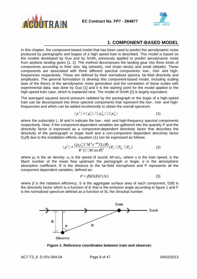
In this chapter, the component-based model that has been used to predict the aerodynamic noise produced by pantographs and bogies of a high speed train is described. This model is based on the models developed by Guo and by Smith, previously applied to predict aerodynamic noise from airplane landing gears [1, 2]. The method decomposes the landing gear into three kinds of components according to their size: big (wheels), mid (main struts) and small (details). These components are associated with three different spectral components: low-, mid- and high-frequencies respectively. These are defined by their normalized spectra, far-field directivity and amplitudes. The general formulation to develop this component-based model, including scaling laws of the theory of the aerodynamic noise generation and the correlation of these scales with experimental data, was done by Guo [1] and it is the starting point for the model applied to the high-speed train case, which is explained next. The model of Smith [2] is largely equivalent.

The averaged squared sound pressure radiated by the pantograph or the bogie of a high-speed train can be decomposed into three spectral components that represent the low-, mid- and high-frequencies and which can be added incoherently to obtain the overall spectrum:

⟩⟨+⟩⟨+⟩⟨=⟩⟨ 2222HML pppp (1)

where the subscripts L, M and H indicate the low-, mid- and high-frequency spectral components respectively. Now, if the component-dependent variables are gathered into the quantity P and the directivity factor is expressed as a component-dependent directivity factor that describes the directivity of the pantograph or bogie itself and a non-component dependent directivity factor D0(θ) due to the installation effects, equation (1) can be expressed as follows:

}{)sin1(

)()(42

0622

002HML

R

PPPMR

DeMcp ++

+=⟩⟨

−

θθρ α

(2)

where ρ0 is the air density, c0 is the speed of sound, M=u/c0, where u is the train speed, is the Mach number of the mean flow upstream the pantograph or bogie, α is the atmospheric absorption coefficient, R is the distance to the far-field microphone and P represents all the component dependent variables, defined as:

)()( StFSDP θβ= (3)

where β is the radiation efficiency, S is the aggregate surface area of each component, D(θ) is the directivity factor which is a function of θ, that is the emission angle according to figure 1 and F is the normalized spectrum defined as a function of St, the Strouhal number.

Figure 1. Reference coordinates between train and o bserver.


ACT-T3_5- D-ISV-004-04 Page 9 of 47 04/02/2013

The Strouhal number (St) is a non-dimensional number that describes oscillating flow mechanism (e.g. vortex shedding) and can be expressed as follows:

U

dfSt

×= (4)

Where f (Hz) is the frequency of the vortex shedding, d (m) is the characteristic dimension of the body inside the flow and U is the flow speed (m/s).

The typical lengths and related Strouhal numbers of each group of component are listed in Table 1. Here a is the average diameter of the cylindrical components, l is the average main dimension of the small details and f is the frequency.

Medium size/ mid-freq. Small size/ high-freq.

Typical length a l

Strouhal number U

afStM

×= U

lfStM

×=

Table 1. Typical dimensions and Strouhal numbers fo r each group of components.

The amplitude of the noise radiated depends on the surface area of each component of the pantograph and bogie, more information about how the surface area of each component is defined is given in sections 3.1 and 4.1.

The radiation efficiency (β) describes how efficiently the motion of the landing gear generates unsteady flows which, in turn, generate propagating sound waves to the far-field. This is an experimental parameter that, in the original model of Guo, depends on the structural design of the landing gear and the relative positions of the different parts of the landing gear (i.e. number of wheels and track alignment angle) but, for its application to the high speed train case, it was reduced to a simple empirical constant β0.

The normalized spectra describe the frequency characteristics of the pantograph/bogie noise in the three frequency domains. Apart from the fact that each of these three groups has specific characteristics, all the normalised spectra achieve a maximum value of unity at a particular value of the Strouhal number St0, given in Table 2, which characterizes the noise generation phenomenon. The spectra drop on both sides of this maximum as the Strouhal number decreases or increases. The normalized spectrum is defined by:

qStB

StAStF

)()( µ

σ

+= (5)

where σ, µ and q are the empirical constants given in Table 2, and A and B are parameters given by:

σµ

σµ −

= qq

Stq

A 0 (6)

µ

σµ

01 Stq

B

−

= (7)


ACT-T3_5- D-ISV-004-04 Page 10 of 47 04/02/2013

Parameter Low freq. components Mid freq. components High- freq. components

St0 1.0 0.3 0.1

σ 4.0 3.0 2.0

µ 2.5 1.5 1.1

q 2.6 4.2 4.2

Table 2. Constants from Guo’s model for the landing gear case [1].

The values of the constants shown in table 2 have been maintained for the application of the model to the high speed train case as first approximation due to the similar order of dimension of the landing gear components compared with the pantograph and bogie components.

For the implementation of the original model developed by Guo for landing gears for the case of pantographs and bogies some simplifications have been assumed. So, the value of α has been set to 0 neglecting the atmospheric absorption that is only significant for long distances between noise source and receiver. The directivity due to the installation effects D0(θ) was assumed as 1, the radiation efficiency β was simplified making β = β0 and the directivity for the pantograph alone was assumed as 1 (omnidirectional source), whereas for the bogie alone it was approximated as 1 from the results obtained from the wind tunnel tests (section 5.2.2). After all these simplifications, equation (2) becomes as follows:

∑+=⟩⟨

componentsiiii StFS

MR

Mcp )(

)sin1(

)(042

622002 β

θρ

(8)

The speed exponent of 6 chosen in the original model (M6) corresponds to the flow speed dependence of a theoretical dipole source, as the noise sources generated due to the vortex shedding from a cylindrical strut. Due to the higher complexity of the pantograph and the bogie, different sound sources can exist and combine with the resulting variation of the speed exponent. The speed exponent was adjusted using the data from the different wind tunnel tests, as shown in sections 3 and 4.

The radiation efficiency (β0i) has been adjusted for the different components defined for the pantograph and bogie cases using the existing and acquired experimental data in order to adjust the changes in the amplitude due to the modification of the speed exponents. Another factor that has been adapted with respect to the original model is the surface area (Si) of each of the components of the pantograph and the bogie.


ACT-T3_5- D-ISV-004-04 Page 11 of 47 04/02/2013

2. PANTOGRAPH CASE

2.1 PANTOGRAPH MODEL

The pantograph is the part of the train most similar to the landing gear in terms of geometry because most of its parts can be approximated as cylindrical or elliptical struts. Moreover, looking at the inflow conditions, the pantograph is also exposed to a relatively clean flow (apart from the lower parts that can be placed inside the boundary layer developed on the train’s roof and the effect of the pantograph recess).

Figure 2 shows how the different parts of the pantograph have been defined into the model. The pantograph is modelled using the mid-frequency source terms for the main struts, control struts and pantograph head and the high-frequency source terms for the details.

Figure 2. Component definition for the pantograph m odel.

The inputs for the model for its application to pantographs are:

• The incident flow speed to each component, in this case assumed as the mean stream flow speed.

• The surface area of each component, based on the length and diameter of the struts, including control struts, main struts and head (the head was modelled as a transverse strut) and the main dimension of the details.

• The tilt angle of the struts. The effect of the tilt angle is based on the Independence Principle [3] so the diameter of the struts is modified according to:

βcos

DD p = (8)


ACT-T3_5- D-ISV-004-04 Page 12 of 47 04/02/2013

where Dp is the projected diameter, D is the original strut diameter and β is the angle formed by the flow direction and the longitudinal axis of the strut.

2.2 ANALYSIS OF EXISTING DATA

During the 15 months of work for the deliverable 3.9 different existing data on sound measurements from full scale pantographs in anechoic wind tunnels provided by the project partners have been analysed in detail. The data used are listed next:

• Analysis 1 - Data in Excel format provided by Deutsche Bahn about noise measurements in the Maibara anechoic wind tunnel for a full scale pantograph.

• Analysis 2 - Report from SNCF and Alstom (ATREBAT project) about noise measurements in an anechoic wind tunnel for a full scale pantograph.

• Analysis 3 - Report from the project DEUFRAKO II about noise measurements in anechoic wind tunnel for a full scale pantograph.

• Analysis 4 - Report from Bombardier about noise measurements in the Audi wind tunnel for a full scale pantograph mounted on a section of train roof.

Although the reports of the analysis 3 and 4 were useful to give improved understanding of the aerodynamic noise mechanisms and the contribution of different parts of the pantograph to the overall noise, they were not used for obtaining the absolute SPL radiated by the pantograph for further comparison with the model.

In the case of the analysis 3, different parts of a full-scale pantograph (head, knee, foot region) were tested at different times by placing them into the core of the jet, but they were not isolated. The overall SPL calculated from the addition of the SPL radiated by the different parts was found to be higher than the overall SPL measured for the same pantograph under similar conditions presented in the analysis 1, where the whole pantograph was introduced into the core of the jet at the same time. It is believed that the increment of the overall SPL in the analysis 3 can be produced by the shear layer effect because the different parts of the pantograph were not isolated during the tests.

In the case presented in the analysis 4, a group of spires was placed upstream of the pantograph in order to generate turbulent inflow, trying to imitate the original flow conditions over a pantograph placed at some point in the middle of the train. The noise generated by the spires masked the noise generated by the pantograph itself so the data recorded by the single microphones used are not suitable for comparison with the model.

Finally, the results after analysing the cases 1 and 2 are shown in sections 3.2.1 and 3.2.2.

2.2.1 Analysis 1 The results presented in this chapter come from measurements made in the RTRI aeroacoustic wind tunnel located in Maibara (Japan) for a full scale pantograph [4]. The data were provided in an Excel file as spectra in A-weighted 1/3 octave bands. The pantograph was exposed to different flow speeds: 115, 170, 230, 280, 330, 350 and 400 km/h. The data used for this analysis were measured by a far-field microphone placed at the line forming an angle of 90 degrees with respect to the flow direction at a distance of 5 m from the pantograph. Background noise correction was applied from the data provided. Both knee upstream and downstream orientations were studied.


ACT-T3_5- D-ISV-004-04 Page 13 of 47 04/02/2013

Figure 3 shows a 3D model of the pantograph used during the wind tunnel experiments and a general view of the experimental set-up [4].

Figure 3. Right - 3D model of the pantograph consid ered in analysis 1. Left – Experimental set-up used during the experiments [4].

In order to verify or to modify the theoretical speed exponent of 6 used in the original formulation, the OSPL (Overall SPL) was plotted against the flow speed. The results after applying curve fitting can be seen in figure 4. The slope of the straight line obtained corresponds to the speed exponent for the noise radiated by the whole pantograph. The speed exponent obtained from the OSPL is 5.6 for the knee upstream, 5.8 for the knee downstream, and from the OASPL (A-weighted OSPL) 6.6 and 6.5 for the knee upstream and downstream respectively.

Figure 4. Variation of the OSPL (left) and the OASP L (right) with the flow speed.

The spectra for the different flow speeds were collapsed using a speed exponent obtained from the OSPL (taking the average speed exponent of 5.7 from a speed exponent of 5.6 for the knee upstream and 5.8 for the knee downstream) according to the next formulation:


ACT-T3_5- D-ISV-004-04 Page 14 of 47 04/02/2013

α)(log10 10, iUicollapsedUi USPLSPL ×−=

where SPLUi is the spectrum for a particular flow speed Ui (m/s) and α is the speed exponent. Figure 5 shows the collapsed spectra for the different flow speeds tested plotted against Strouhal number. It can be noticed that the curves do not match equally in the whole Strouhal number range. It can be inferred that different speed exponents will apply in different Strouhal number regions and, therefore, in different frequency regions. In order to study the speed exponent that minimised the differences between the collapsed spectra across the frequency (Strouhal number) range, different speed exponents were tried in the range between 5 and 7 for steps of 0.1 for the central frequency of each 1/3 frequency band, the exponent that provided the minimum value of the standard deviation for each frequency was chosen. The results obtained are shown in figure 6.

Figure 5. Collapsed spectra for the upstream (left) and downstream (right) knee

orientations.

Figure 6. Dependence of the speed exponent with the frequency for the upstream (left) and downstream (right) knee cases.


ACT-T3_5- D-ISV-004-04 Page 15 of 47 04/02/2013

There is a considerable fluctuation of the optimum speed exponent across the frequency range that makes difficult to select consistently different speed exponents for the low-, mid- and high- spectral components. For this reason, the average value of 5.7 (taking the speed exponents of 5.6 and 5.8 for knee upstream and downstream respectively) was selected for the comparisons with the measurements.

Due to the change of the speed exponent respect to the original model, the radiation efficiency for the mid-frequency (main struts, controls struts and head) and high- frequency (details) components was modified in order to obtain the correct spectral amplitude. So, the values of the radiation efficiency chosen were 3.0 x 10-10 for the middle size components (head, main struts and control struts) and 6.4 x 10-7 for the details.

Figure 7 and figure 8 show the results of comparing the wind tunnel measurements with the output from the model for different flow speeds for the knee upstream and downstream, using the modified speed exponent and radiation efficiency. The contribution of each independent component is included (main struts, control struts, head and details) as well as the overall spectrum predicted resulting from the addition of the spectrum predicted for each individual component.


ACT-T3_5- D-ISV-004-04 Page 16 of 47 04/02/2013

Figure 7. Comparison between measurements and model for the pantograph knee placed upstream.


ACT-T3_5- D-ISV-004-04 Page 17 of 47 04/02/2013

Figure 8. Comparison between measurements and model for the pantograph knee placed downstream.


ACT-T3_5- D-ISV-004-04 Page 18 of 47 04/02/2013

A good agreement between the model output and the measurements was obtained both for the amplitude and the spectral shape. However, measured data show the appearance of distinguishable peaks at some frequency bands probably generated by the flow interaction with the horns and other complex structures of the pantograph head.

Figure 9 shows the differences between the OASPL measured and predicted for the different flow speeds. This indicates a slight under-prediction due to the omission of the tonal peaks. It must be pointed out that these tonal peaks can be overrepresented in the wind tunnel tests compared with in-situ tests due to the disturbed inflow and the Doppler effects in the latter case.

Figure 9. Comparison between the OASPL from the win d tunnel tests and from the prediction model for different flow speed for the p antograph knee downstream (left) and

upstream (right).

2.2.2 Analysis 2 In this section, results are from measurements carried out in an open jet anechoic wind tunnel for a full scale pantograph tested for different flow speeds: 40, 61, 81 and 98 m/s [5]. These were analysed and compared with the prediction model. The results were provided as A-weighted SPL spectra in 1/3 octave bands measured with a microphone placed at 6 m from the centre of the pantograph at an angle of 90 degrees with respect to the flow direction, so convective amplification can be neglected. The pantograph knee was placed upstream and it is believed that the whole pantograph was placed into the core of the jet (apart from the lower part) although no flow measurements were done. The position of the pantograph horn inside the jet core was checked using smoke for flow visualization. For comparison with the model it should be considered that, below 200 Hz, the background noise level of the wind tunnel was predominant. Figure 10 shows the experimental set-up used.


ACT-T3_5- D-ISV-004-04 Page 19 of 47 04/02/2013

Figure 10. Left – Picture of the experimental set-u p. Right – Sketch of the pantograph and microphone

positions inside the test section.

The same analysis as in section 3.2.1 was applied to this case. Figure 11 shows the straight line obtained after applying curve fitting to the OSPL and OASPL against the flow speed. This time, the resultant speed dependence was 5.7 for the OSPL and 6.2 for the OASPL.

Figure 11. Variation of the OSPL (left) and the OAS PL (right) with the flow speed.

Figure 12 shows the spectra for the different flow speeds collapsed for the 5.7 power of the flow speed. Fluctuations in the speed dependence were found (figure 10), but smaller than for the analysis 1.


ACT-T3_5- D-ISV-004-04 Page 20 of 47 04/02/2013

Figure 12. Left - Collapsed spectrum for the pantog raph using a speed exponent of 5.7. Right - Dependence of the speed exponent with the f requency.

After applying a speed dependence of 5.7 and calibrating the radiation efficiency for each of the pantograph components (9.4 x 10-10 for the mid- size components and 1.3 x 10-6 for the details), the comparison between model and experiments is shown in figure 11.


ACT-T3_5- D-ISV-004-04 Page 21 of 47 04/02/2013

Figure 13. Comparison between measurements and mode l.

A good agreement between model and measurements was achieved with just two spectral features that show disagreement: First, below 200 Hz the amplitude of the measured spectrum is higher than the predicted from the model due to the effect of the wind tunnel background noise (figure 14 shows the comparison between pantograph and background noise for a flow speed of 98 m/s), making the comparison not valid for this frequency range. Second, the appearance of some peaks, probably due the effects of the horn/flow interaction, was not predicted by the model.

Figure 14. Comparison between pantograph and backgr ound noise for a flow speed of 98 m/s. dB expressed using an arbitrary reference [5].

It must be noticed that the values of the radiation efficiency are not the same for the analysis 1 and 2. When the data from the measurements for both pantographs was compared for the same flow speed, significantly higher values (>5 dB) was obtained for analysis 2 even if it is geometrically simpler pantograph. The origin of this disagreement may be in the experiments.


ACT-T3_5- D-ISV-004-04 Page 22 of 47 04/02/2013

Due to the big dimension of the anechoic wind tunnel that ensure the whole pantograph was placed inside the core of the jet, the reference case finally chosen to obtain the inputs for the Acoutrain software was the tests from analysis 1 presented in section 3.2.1.

2.3 CONCLUSIONS AND MODEL LIMITATIONS From the good agreement found in the comparison between the model predictions and the experimental data analysed it can be concluded that the component-based model proposed is reliable to predict the aerodynamic noise radiated by a generic pantograph and it is then suitable to provide the Sound Power Levels (PWL) to be used as inputs for the Acoutrain software.

Despite that, it is important to state the limitations found in its application:

• The directivity of the pantograph components was assumed to be omnidirectional. No useful data to validate or contradict this assumption was provided.

• The appearance of peaks at specific frequencies across the spectrum, probably by the effect of the flow interaction with the horns and other complex structures in the pantograph head, shown that more complexity in the model prediction for the head component should be added in order to fit the output to these spectral features.

• The radiation efficiency of each component of the model was calibrated using the measurements for the whole pantograph. Because no noise spectrum from each specific component was provided, it was not possible to calibrate the model constants to adjust the spectral shape of each component, so the same values of the constants as the original model were used.

3. BOGIE CASE

3.1 BOGIE MODEL

Bogies from a high speed train present a more complex geometry than pantographs, generating flow interactions between components of the bogie that in most cases has a turbulent nature. In addition, the flow character is more complex than for the pantograph, with a higher degree of large scale vortices in the inflow. Nevertheless, for the model developed here, all the bogie components have been modelled as cylindrical or elliptical transverse struts (transverse to the flow direction or train motion direction) and the effect of turbulent flow was not taken into account, only considering clean inflow at different flow speeds.

Figure 15 shows how the different parts of the bogie have been defined in the model. The bogie is modelled using the mid-frequency source terms for the side frames, wheels, dampers, transverse members, brake disks, gear box, motor and downstream forward-facing step of the bogie cavity and the high-frequency source terms for the different size details.


ACT-T3_5- D-ISV-004-04 Page 23 of 47 04/02/2013

Figure 15. Component definition for the bogie model .

The inputs for the model for its application to bogies are:

• The local incident flow speed to each component. This flow speed was roughly approximated from the measurements of mean flow speed done using a Pitot tube at different positions around the bogie in the tests described in the next section.

• The surface area of each component, based on the length, diameter and/or main dimension of each component.

3.2 EXPERIMENTAL DESIGN

For the bogie case, no existing data was available for comparison with the prediction model and its calibration. For this reason, experiments were designed and carried out using a 1/10 scale bogie mock-up, measuring the noise radiation under different flow speeds. The measurements were done in the Institute of Sound and Vibration Research (ISVR) open jet anechoic wind tunnel. This facility provides a high speed flow with low background noise and low turbulence level. Figure 16 shows the rear view of the experimental set-up.

A scaling factor of 1/10 was chosen to ensure that the bogie model was placed inside the core of the jet avoiding the effects of the shear layer impinging on the bogie mock-up The use of a scale factor of 1/10 implies that the frequencies of the measurements are 10 times higher than at full scale while the sound pressure amplitudes are reduced.

The Reynolds numbers achieved during the experiments are considerably lower than for a full scale bogie. The flow regime around cylindrical objects is expected to be in the subcritical range when it can achieve the critical or supercritical range for a full scale bogie. Nevertheless, all the cylindrical shafts are placed inside the cavity and partially covered by other objects (motor, brake disks, etc) so, as shown in the results from the experiments, no strong peak related with vortex shedding from the axle could be found.


ACT-T3_5- D-ISV-004-04 Page 24 of 47 04/02/2013

For non-cylindrical objects (disks, rectangular and square objects, etc) like the wheels, motor, gear boxes, brake systems… the dependency of the noise spectral shape with the Reynolds number is expected to be lower because the flow separation occurs in the leading edge for all cases.

Figure 16. Rear view of the experimental set-up.

The contraction nozzle, shown in figures 15 and 16, provides a smooth laminar flow. Different flow speeds (25 m/s, 40 m/s and a maximum flow speed of 50 m/s) were used during the experiments depending on the configuration under test. The components used for the experiments (see figure 17) were attached to a stiff panel made of plywood (1.2 m by 0.5 m) that simulates the floor of the real train. This rigid panel was surrounded by an acoustic baffle in order to minimise the noise generated by flow interaction with the edges of the panel. These two structures were not directly connected in order to avoid the transmission of vibration from the panel to the baffle and vice versa. The acoustic baffle was constructed of an aluminium sheet covered in dense acoustic foam on the flow-facing side of the baffle. This isolated the baffle from both the acoustic field and the turbulence in the flow. The baffle was aligned flush with the edge of the nozzle to ensure smooth flow delivery and avoid flow separation. The centre of the bogie model under test was aligned with the centreline of the nozzle in such a way that the flow can be considered symmetric on both sides of the bogie model.

Figure 17. Front view of the experimental set-up.


ACT-T3_5- D-ISV-004-04 Page 25 of 47 04/02/2013

All the measurements were made using seven microphones placed in the far-field of the component under test, attached to an arc shaped metal structure. The metal structure, placed above the acoustic baffle (figure 18), was used to hold the far-field microphones. All the microphones were levelled with respect to the position of the mock-up so the different positions of the microphones in the arc array allowed the sound radiation to be measured at different angles (details are given in section 5.2.1, table 5) of propagation for a subsequent study of the directivity of the noise sources. Figure 18 shows the location of the arc array and how the microphones were attached.

Figure 18. Arc array composed by seven microphones used to measure the noise radiated by the components under test.

A phased array composed of 49 microphones was used to obtain noise maps using beam-forming techniques to allow noise source localization. Figure 19 shows the phased array set-up, where the array was placed at a distance of 76 cm from the baffle with its centre aligned with the centre of the bogie model.


ACT-T3_5- D-ISV-004-04 Page 26 of 47 04/02/2013

Figure 19. Phased array used for noise mapping and source localization using beam-forming techniques.

Finally, the local flow speed at different positions around, above and inside the bogie model was measured using a Pitot tube connected to an analogue manometer. Figure 20 shows the set-up used for these measurements. A tuft was attached to the Pitot tube in order to have an estimation of the flow behaviour at the different points where the measurements were done.

Figure 20. Set-up for the Pitot tube measu rements.

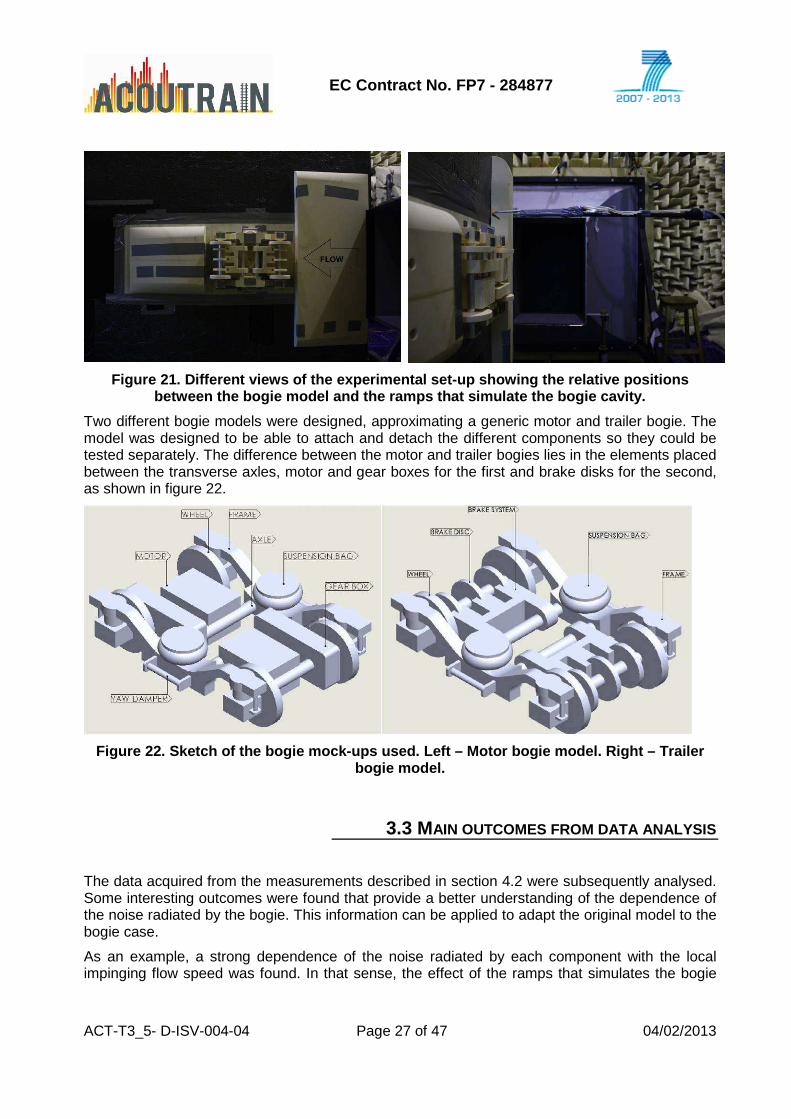
In order to simulate the inflow conditions to the bogie when this is installed in a real train, two ramps were used. Figure 21 shows two different views of these ramps and their relative position with respect to the bogie mock-up. The size of the ramp steps was also adapted to the 1/10 scale. The upstream ramp was designed to avoid flow separation and to provide clean and smooth flow to the upstream wheelset components.


ACT-T3_5- D-ISV-004-04 Page 27 of 47 04/02/2013

Figure 21. Different views of the experimental set- up showing the relative positions between the bogie model and the ramps that simulate the bogie cavity.

Two different bogie models were designed, approximating a generic motor and trailer bogie. The model was designed to be able to attach and detach the different components so they could be tested separately. The difference between the motor and trailer bogies lies in the elements placed between the transverse axles, motor and gear boxes for the first and brake disks for the second, as shown in figure 22.

Figure 22. Sketch of the bogie mock-ups used. Left – Motor bogie model. Right – Trailer bogie model.

3.3 MAIN OUTCOMES FROM DATA ANALYSIS

The data acquired from the measurements described in section 4.2 were subsequently analysed. Some interesting outcomes were found that provide a better understanding of the dependence of the noise radiated by the bogie. This information can be applied to adapt the original model to the bogie case.

As an example, a strong dependence of the noise radiated by each component with the local impinging flow speed was found. In that sense, the effect of the ramps that simulates the bogie


ACT-T3_5- D-ISV-004-04 Page 28 of 47 04/02/2013

cavity cannot be neglected because they shield some parts of the bogie with respect to the incident flow, decreasing the flow speed.

Figure 23 shows the comparison of the noise spectra measured by the microphone number 3 (the axis of this microphone formed an angle close to 90 degrees relative to the flow direction, so the convective amplification can be neglected) for the baffle alone, the baffle plus both ramps, and baffle, ramps and trailer or motor bogie. The measurements with the baffle alone can be taken as the background noise due to the experimental set-up, including wind tunnel noise and instrumentation noise. In order to obtain the noise from the ramps, which can be related with the noise generated in the real train by the cavity itself, the background noise correction was done by subtracting the noise of the baffle from the noise of both ramps plus baffle.

Figure 23. Background noise and dynamic range durin g the measurements for the flow speed of 25 and 50 m/s.

From the subtraction of the noise of the upstream ramp from the noise of both ramps the noise due to the downstream ramp can be obtained. Figure 24.a shows how the noise from both ramps is higher than the noise from the upstream ramp alone in most of the frequency range. This noise is probably generated by the vortex shedding from the upstream ramp trailing edge impinging on the downstream ramp forward facing step. The noise mapping presented in figure 24.b shows how the higher contribution is coming from the downstream ramp forward facing step.


ACT-T3_5- D-ISV-004-04 Page 29 of 47 04/02/2013

Figure 24 . a) Left – Noise spectrum from ramps. b) Right – Noi se map for the octave band of frequency of 4 kHz.

The noise was measured for four different configurations of the trailer bogie. The first configuration is the bogie model just with the axles, wheels and frames but without any brake system. Next, the front brake system was added, and then the rear brake system was added so the whole trailer bogie was tested and finally the front brake system was removed so that only the rear system was tested. Results are gathered in figure 25.b.

Figure 25.b shows the noise spectra for each of these configurations for a flow speed of 50 m/s. In the lower part of the frequency range the effect of adding the brake system decreases slightly the noise generated by the axles and wheels. At higher frequencies noise coming from the front brake system is predominant, producing three broad peaks around 2.5 kHz, 3.7 kHz and 7 kHz. These results are in good agreement with the noise map shown in figure 24.a for the octave band of 4 kHz, where the noisiest part of the bogie model coincides with the front wheel set. As a result of this analysis of the trailer bogie, the brake system can be identified as the most significant noise source inside the front axle above 2 kHz.

Figure 25. a) Left – Noise map for the octave band of frequency of 4 kHz. b) Right – Noise spectrum from different trailer bogie configuration s.


ACT-T3_5- D-ISV-004-04 Page 30 of 47 04/02/2013

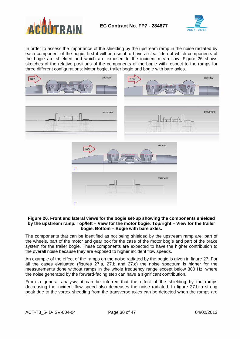
In order to assess the importance of the shielding by the upstream ramp in the noise radiated by each component of the bogie, first it will be useful to have a clear idea of which components of the bogie are shielded and which are exposed to the incident mean flow. Figure 26 shows sketches of the relative positions of the components of the bogie with respect to the ramps for three different configurations: Motor bogie, trailer bogie and bogie with bare axles.

Figure 26. Front and lateral views for the bogie se t-up showing the components shielded by the upstream ramp. Top/left – View for the motor bogie. Top/right – View for the trailer

bogie. Bottom – Bogie with bare axles.

The components that can be identified as not being shielded by the upstream ramp are: part of the wheels, part of the motor and gear box for the case of the motor bogie and part of the brake system for the trailer bogie. These components are expected to have the higher contribution to the overall noise because they are exposed to higher incident flow speeds.

An example of the effect of the ramps on the noise radiated by the bogie is given in figure 27. For all the cases evaluated (figures 27.a, 27.b and 27.c) the noise spectrum is higher for the measurements done without ramps in the whole frequency range except below 300 Hz, where the noise generated by the forward-facing step can have a significant contribution.

From a general analysis, it can be inferred that the effect of the shielding by the ramps decreasing the incident flow speed also decreases the noise radiated. In figure 27.b a strong peak due to the vortex shedding from the transverse axles can be detected when the ramps are


ACT-T3_5- D-ISV-004-04 Page 31 of 47 04/02/2013

not attached. Once the ramps are included in the test, the inflow conditions experienced by the transverse axles change and the peak in the spectrum disappears.

Figure 27. Noise spectra measured with and without ramps for the next configurations: a) Top/Left – Trailer bogie. b) Top/Right – Just frame s, transverse axles and wheels. c)

Bottom – Motor bogie.

The effect of the side frames and lateral dampers has not been assessed yet. Figure 28 shows the spectrum measured with the ramps plus side frames and plus lateral dampers attached to the test panel and the spectrum obtained just using both ramps. If they are compared it is not possible to find any significant difference between them and, therefore, the noise radiated by the side frames and dampers cannot be isolated from the noise from the ramps.

In the case tested, the side frames and lateral dampers were shielded by the upstream ramp the width of which is higher than the nozzle width in order to avoid noise from the edges of the upstream ramp. This is not the situation that can be expected in the real case where the frames and dampers are exposed to the side flow of the train.


ACT-T3_5- D-ISV-004-04 Page 32 of 47 04/02/2013

Figure 28. Spectrum radiated by the side frames and lateral da mpers for a flow speed of 25 m/s (left) and 50 m/s (right).

Following the same procedure as for the pantograph case, the speed exponent of the whole trailer and motor bogie was calculated. Figure 29 shows the variations of the OSPL with the flow speed (three different flow speeds were tested: 25, 40 and 50 m/s). The slope of the fitted straight line provides the speed dependence coefficient, 6.2 for the trailer bogie and 6.3 for the motor bogie.

Figure 29. Variation of the OSPL with the flow spee d for the trailer (left) and motor (right) bogie.

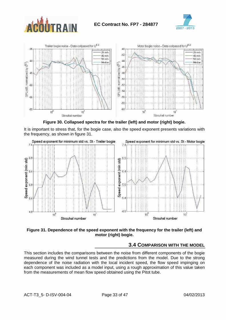
Figure 30 shows the collapsed spectrum for the three flow speeds tested using a speed exponent of 6.2 for both the trailer and the motor bogie.


ACT-T3_5- D-ISV-004-04 Page 33 of 47 04/02/2013

Figure 30. Collapsed spectra for the trailer (left) and motor (right) bogie.

It is important to stress that, for the bogie case, also the speed exponent presents variations with the frequency, as shown in figure 31.

Figure 31. Dependence of the speed exponent with th e frequency for the trailer (left) and motor (right) bogie.

3.4 COMPARISON WITH THE MODEL This section includes the comparisons between the noise from different components of the bogie measured during the wind tunnel tests and the predictions from the model. Due to the strong dependence of the noise radiation with the local incident speed, the flow speed impinging on each component was included as a model input, using a rough approximation of this value taken from the measurements of mean flow speed obtained using the Pitot tube.


ACT-T3_5- D-ISV-004-04 Page 34 of 47 04/02/2013

Figure 32 shows the position of the measurement points and the flow speed measured at each of those positions. The flow speeds chosen as inputs to the prediction model for the wheels, side frames and axle, shown in figure 32, were chosen by proximity between the measurement point and each component.

Figure 32. Sketch showing the positions where the P itot tube was placed and the flow speed measured at each position.

For simplicity, the values of the incident flow speed chosen for each component are provided in table 3.

Component Flow speed (m/s)

Mean flow 50

Transverse axles 17

Wheels 48

Side frames 36

Brake disks 48

Rear step 30

Table 3. Incident flow speed chosen for each compon ent from the Pitot tube measurements.

A first comparison shows (figure 33) the noise spectrum from the side frames when measured without ramps, so they are exposed to an incident flow speed equal to the mean flow speed (50 m/s for this case). The measured spectrum has been corrected for background noise – at most frequencies this correction is modest (mostly less than 1 dB above 500 Hz). Differences in amplitude are relatively small but there are some differences in the spectral shape that imply that the method of modelling the non-cylindrical parts should be reviewed.


ACT-T3_5- D-ISV-004-04 Page 35 of 47 04/02/2013

Figure 33. Comparison between model and measurement s for the side frames exposed to

a mean flow speed of 50 m/s (no ramps attached).

When the ramps are included in the measurements, the side frames are shielded by them. Figure 34 shows how the model fits better to the experiments when the local incident flow speed is included as an input for each component. Anyway, the measurement of the side frame noise in the wind tunnel experiment do not reflect the real conditions because they were shielded by the upstream ramp, unlike the real case where they are exposed to the train side flow. The background noise correction here is more substantial than in the previous case, typically 5 dB.

Figure 34. Comparison between the measured spectrum from the side frames with the ramps attached (mean flow speed of 50 m/s) and outp ut from model using as inputs the

mean flow speed and the measured local incident flo w speed (36 m/s).

Figure 35 shows the results after adding more components to the bogie model (axles and wheels) when the ramps are not included.


ACT-T3_5- D-ISV-004-04 Page 36 of 47 04/02/2013

Figure 35. Comparison between model and measurement s for the side frames plus wheels sets exposed to a mean flow speed of 50 m/s (no ram ps attached).

Two strong peaks appear in the measured spectrum due to the vortex shedding from the transverse axles. For this case, the spectrum predicted by the model does not show those narrow peaks. The frequency where the maximum value of the predicted spectrum is placed does not match with the frequency for the maximum value of the measured spectrum.

When the ramps are included, the measured spectrum has a flatterer shape and the peaks from the vortex shedding from the transverse axles disappear as is shown in figure 36. Again, the maximum for both spectra, measured and predicted, do not match at the same frequency.

Figure 36. Comparison between the measured spectrum from the side frames plus wheel sets with the ramps attached (mean flow speed of 50 m/s) and output from model using as

inputs the mean flow speed and the measured local i ncident flow speed (36 m/s for side frames, 17 m/s for transverse axles and 45 m/s for wheels).

Finally, the comparison for the whole trailer bogie is shown in figure 37.


ACT-T3_5- D-ISV-004-04 Page 37 of 47 04/02/2013

Figure 37. Comparison between the measured spectrum from the trailer bogie with the ramps attached (mean flow speed of 50 m/s) and outp ut from model using as inputs the

local incident flow speed for each component.

The disagreement at low frequencies can be due to the effect of the experiment set-up into the measured noise (background noise) but also the model is underestimating the noise from the forward-facing step introduced by the downstream ramp. In the rest of the spectrum the differences between model and measurements are smaller than 10 dB. Considering the contribution of each individual component, it should be noticed how the contribution from the wheels is overestimated, being much more significant than the contribution from the brake disks, which is in disagreement with what was found in the experiments.

For the model predictions it was considered that the whole surface area of each element was exposed to the incident flow speed. That is not true in the case, for example, of the wheels and brake disks because approximately half of the surface area of these components is shielded by the upstream ramps. Applying this correction in the surface area exposed to the main flow, a reduction of 3 dB in the predicted spectrum is expected. Even so, a review of how the non-cylindrical objects are modelled is necessary.

3.5 CONCLUSIONS AND MODEL LIMITATIONS The comparison between the wind tunnel experiments and the predictions from the model has shown that the current model is not yet suitable for aerodynamic noise prediction from bogies. Next actions are proposed for further model development in order to improve its performance:

• Square, rectangular and other non-cylindrical components have been modelled as cylindrical. This fact can lead to differences in the noise spectrum shape and amplitude predicted.

• It was found that there is a strong dependence between the local incident flow speed on each component and the noise radiation. The flow speeds used as model inputs were


ACT-T3_5- D-ISV-004-04 Page 38 of 47 04/02/2013

approximated from the mean flow speed measurements carried out using a Pitot tube. This approximation introduces a non-negligible uncertainty in the spectrum calculations.

• No information about turbulence intensity in the flow around the bogie components was included. Due to the geometrical complexity of the bogie, a turbulence factor can be included into the model for higher accuracy.

• The PWL for each individual bogie will depend on its position on the train. The flow speed will be greatest for the leading bogie and will be reduced for other bogies due to the growth of the TBL and the turbulence generated from the interaction between the preceding bogies and the flow. This effect was not simulated in the experiments.

As alternative input for the Acoutrain project, the sound power level and directivity calculated from the wind tunnel measurements is proposed.

4. INPUT TO THE ACOUTRAIN SOFTWARE

4.1 PANTOGRAPH

The PWL spectra for different train speeds are provided in table 4. These spectra can be associated in the Acoutrain software as the sound power level of a pantograph source. The directivity factor is 1, assuming that the pantograph is an omnidirectional source. All the spectra were calculated using the component-based model described in this report using a speed exponent of 5.7. To allow for other pantograph designs the component-based model could be used with different input parameters to generate equivalent spectra. In order to better interpret the results in table 4, an uncertainty of +/- 5 dB should be considered for the frequency bands considered, based on the results presented in figures 7 and 8. In terms of the overallPWL, a margin of +/- 2 dB can be considered.

Frequency (Hz)

20 25 32 40 50 63 80 100 125 160 200

Speeds

(km/h)

100 53.7 57.2 60.6 63.8 66.7 69.2 71.4 73.1 74.4 75.3 75.8

150 57.2 61.0 64.6 68.1 71.4 74.5 77.3 79.8 81.9 83.5 84.7

200 59.6 63.4 67.2 70.8 74.4 77.7 80.9 83.8 86.4 88.5 90.3

250 61.4 65.2 69.0 72.8 76.5 80.0 83.4 86.5 89.4 91.9 94.1

300 62.8 66.7 70.5 74.3 78.1 81.7 85.2 88.6 91.7 94.5 96.9

350 64.0 67.9 71.8 75.6 79.4 83.1 86.7 90.2 93.4 96.4 99.1

400 65.0 69.0 72.8 76.7 80.5 84.3 87.9 91.5 94.9 98.0 100.9


ACT-T3_5- D-ISV-004-04 Page 39 of 47 04/02/2013

Frequency (Hz)

250 315 400 500 630 800 1000 1250 1600 2000

Speeds

(km/h)

100 76.0 76.0 75.8 75.4 74.9 74.2 73.4 72.5 71.5 70.5

150 85.5 85.9 86.1 86.0 85.7 85.3 84.8 84.1 83.3 82.3

200 91.6 92.5 93.0 93.2 93.2 92.9 92.6 92.1 91.4 90.6

250 95.8 97.1 98.0 98.5 98.7 98.7 98.5 98.1 97.6 96.9

300 99.0 100.7 101.9 102.7 103.1 103.2 103.2 102.9 102.5 101.9

350 101.5 103.4 104.9 106.0 106.7 107.0 107.1 106.9 106.6 106.1

400 103.5 105.7 107.4 108.7 109.6 110.1 110.4 110.3 110.1 109.7

Frequency (Hz)

2500 3150 4000 5000 6300 8000 10000 12500 16000 20000

Speeds

(km/h)

100 69.3 68.1 66.9 65.5 64.2 62.7 61.3 59.8 58.3 56.7

150 81.3 80.2 79.1 77.9 76.6 75.3 73.9 72.4 71.0 69.5

200 89.7 88.7 87.6 86.5 85.3 84.0 82.7 81.3 79.9 78.5

250 96.1 95.2 94.2 93.1 92.0 90.8 89.5 88.2 86.8 85.4

300 101.2 100.4 99.5 98.5 97.4 96.2 95.0 93.8 92.4 91.0

350 105.5 104.8 103.9 103.0 101.9 100.8 99.7 98.4 97.1 95.8

400 109.2 108.6 107.8 106.9 105.9 104.8 103.7 102.5 101.2 99.9

Table 4. Pantograph PWL predicted for different tra in speeds.

4.2 BOGIE

4.2.1 Sound power The PWL has been estimated from the SPL measured at seven different positions placed in a plane parallel to the acoustic baffle and aligned with the centre line of the bogie (the acoustic centre is assumed to be located at the centre point of the bogie). These measurements were carried out for a flow speed of 50 m/s.


ACT-T3_5- D-ISV-004-04 Page 40 of 47 04/02/2013

Figure 38 . Sketch of the far-field microphone positions respec t to the bogie position. Θi is the radiation angle.

Table 5 shows the distance to the bogie and radiation angle for each of the seven microphones used.

Microphone Distance(m) Angle (Degrees)

1 1.99 16.1

2 2.02 4.3

3 2.05 -5.6

4 2.09 -15.8

5 2.12 -25.3

6 2.16 -36.0

7 2.21 -45.4

Table 5. Distance to the bogie and radiation angles for each of the microphones used.

Next formula has been used taken as a reference the procedure followed in the ISO 3745 [6] for the calculation of the PWL of noise sources from measurements in anechoic chamber over a reflecting plane.

×+=

010log10

S

SLL pfW


ACT-T3_5- D-ISV-004-04 Page 41 of 47 04/02/2013

where is the spatial average sound pressure level at the surface of measurements in 1/3 octaves (dB, ref 2x10-5 Pa), S is the surface area of measurement (half a sphere for this case where the baffle is assumed to be an infinite reflecting plane) and S0 is the reference surface area (1 m2). For a flow speed different from 50 m/s, the PWL was adjusted using the speed dependence factor of 6.2 for both trailer and motor bogie.

It must be noticed that the effects of the model scaling must to be corrected in terms of the amplitude of the noise radiation, due to the difference of surface area exposed to the flow, and frequency, accounting for the shift in the vortex shedding frequency due to the difference in the characteristic dimension of the object. For this reason, the amplitude of the noise spectra measured was multiplied by a factor of L2, L being the scaling factor for the bogie model (L=10), and the frequency was divided by L. Also, a variation in the vortex shedding frequency is expected with the variation of the flow speed. Because the PWL spectra for the different flow speeds are calculated from the measured PWL spectrum for a flow speed of 50 m/s applying the appropriate scaling laws, the frequency vector associated with these measurements was also multiplied by a factor of (Ui/50), where Ui is the flow speed at which the PWL is estimated, in order to account for the variations in the vortex shedding frequency.

The table 6 shows the PWL scaled for different train speeds for a single bogie (calculated by averaging the PWL from the motor and the trailer bogie) that can be used as inputs in the Acoutrain software. The differences between the sound power radiated by the motor bogie and the trailer bogie mock-up are lower than 2 dB along the whole frequency range, being therefore smaller than the uncertainty associated to the PWLspectra. For this reason, the differences between the noise radiated by the motor and the trailer bogie are not significant and an average PWR is presented in table 6. It must be pointed out that both trailer and motor bogie models were exposed to the mean flow speed during the experiments and the effect of their position on the train was not taken into account. Therefore, the differences in the noise radiation are just due to the geometrical differences between motor and trailer bogie models.

Looking at the results presented in figure 39, the spectral results presented in table 6 should be considered to have an uncertainty of +/-4 dB for the frequency range up to 630 Hz. At higher frequencies the uncertainty is unknown but the levels are lower than those of other sources. In terms of the OASPL (taking into account a frequency range up to 630 Hz and just considering the train speeds of 300 and 350 km/h where the aerodynamic sources are predominant), a margin of +/- 2.5 dB can be considered.

Frequency (Hz)

20 25 32 40 50 63 80 100

Speeds

(km/h)

150 95.2 95.3 94.5 94.7 94.5 94.8 94.8 94.0

180 99.7 100.2 100.1 99.3 99.7 99.3 100.0 99.5

200 102.7 102.8 103.2 102.3 102.3 102.3 102.4 102.8

250 108.4 108.7 108.8 109.2 108.3 108.3 108.3 108.4

300 112.3 113.5 113.5 113.8 114.0 113.2 113.3 113.2

350 116.7 117.0 117.7 117.7 118.2 117.9 117.1 117.6

400 121.3 119.9 121.1 121.3 121.4 121.9 121.0 121.0

pfL


ACT-T3_5- D-ISV-004-04 Page 42 of 47 04/02/2013

Frequency (Hz)

125 160 200 251 315 400 500 630

Speeds

(km/h)

150 94.1 93.7 93.6 92.7 91.4 90.0 89.9 89.4

180 98.8 99.0 98.5 98.7 97.0 96.0 94.8 94.8

200 101.9 101.9 101.7 100.9 101.2 99.4 97.9 97.7

250 108.8 107.9 107.9 107.6 107.0 107.1 105.3 103.9

300 113.5 113.5 112.6 112.8 112.4 112.3 111.4 110.1

350 117.2 118.0 117.3 116.8 116.9 116.3 116.6 114.6

400 121.0 121.1 121.5 120.5 120.6 120.3 119.6 119.9

Frequency (Hz)

800 1000 1250 1600 2000 2500 3150 4000

Speeds

(km/h)

150 87.3 85.4 83.0 79.4 58.4 * * *

180 93.9 91.8 89.9 87.2 83.3 * * *

200 97.4 95.6 93.7 91.4 88.2 * * *

250 103.7 103.3 101.5 99.6 97.4 94.1 * *

300 108.7 108.6 108.1 106.0 104.1 101.7 98.1 *

350 113.7 112.7 112.7 111.6 109.5 107.6 104.8 100.6

400 118.0 116.6 116.3 116.0 114.3 112.3 110.1 106.9

Table 6. Bogie PWL obtained from the average of the PWL from the motor and the trailer bogie using the data from the wind tunnel e xperiments.

4.2.2 Directivity First, a correction for the different distances between bogie and each microphone was applied (the radius of the arc was not fixed respect to the bogie position):

where di is the distance between the bogie and the ith microphone, and dref is the minimum distance between the closest microphone to the bogie and the bogie. The corrected SPL is obtained by adding the correction to the measured SPL:

The directivity is normalized so its values will lie in the range between 0 and 1:

×= 2

2

10log10ref

icorrection d

dL

correctionmeasuredcorrected LSPLSPL +=

2max,

2,

k

ki

p

pD =


ACT-T3_5- D-ISV-004-04 Page 43 of 47 04/02/2013

where p2i,k is the squared sound pressure for the ith angle and the kth 1/3 octave band, and p2

max,k

is the maximum value of the squared sound pressure in the kth 1/3 octave band.

All the values of directivity obtained using the previous equation, either for the trailer or the motor bogie, lie between 0.9 and 1, which expressed in dB means a maximum difference of 0.5 dB. The bogie source can therefore be approximated as an omnidirectional point source without significant error.

4.2.3 Validation In order to ensure that the PWL data given in section 5.2.1 obtained from the wind tunnel measurements using a1/10 scale bogie mock-up is valid for the full scale bogie, comparisons are made with measured data. The SPL at 25 m from the train was calculated using the PWL obtained from the wind tunnel experiments and this was compared with the SPL obtained from pass-by field measurements for a real train for different train speeds (200, 250, 300 and 350 km/h) [7]. It can be assumed that the noise generated in the low frequency part of the spectrum (below 2 kHz approximately, depending on the train speed) is dominated by aerodynamic noise mainly generated by the bogies. It must be noticed that the spectra shown in [7] are the time averaged spectra for the pass-by measurement time. The number of bogies is 13 for the whole train, whereas the number of pantographs is 2 (one raised and one lowered). Due to the time integration used for obtaining the spectra, a bigger contribution of the bogies to the overall aerodynamic noise is expected even though the temporal event due to a pantograph can have a higher level compared with an individual bogie.

To generate the pass-by spectra from the PWL obtained from the wind tunnel tests a Matlab code was developed taking in account the influence of the 13 bogies (4 motor bogies and 9 trailer bogies) in the pass-by noise, including convective amplification, Doppler frequency shift and the effect of retarded time in the calculations. The results were validated against the calculation done with the Acoutrain software using the same PWL inputs. For the comparison with the pass-by measurements the TEL (Transit Exposure Level) was obtained for the predicted spectrum according to the expression provided in the ISO 3095 [8]. No difference was allowed for between the leading bogie and subsequent bogies.

Figure 39 shows the results from the comparison between the pass-by spectra calculated using the PWL obtained from the wind tunnel test against the pass-by measurements for a real train. A good agreement was found both for amplitude and shape of the spectra. The speed exponent is slightly higher for the data from the wind tunnel test, probably due to the influence of other sound sources during the pass-by measurements.


ACT-T3_5- D-ISV-004-04 Page 44 of 47 04/02/2013

Figure 39. Comparison between the SPL spectra measu red during pass-by field measurement for a full scale train passing through at different speeds [7] and the SPL spectra obtained from the wind tunnel tests for the same flow speed after applying the

scaling factors.

5. CONCLUSIONS

A component based semi-empirical model was adapted from Guo’s model, originally used for landing gear aerodynamic noise prediction, to the high speed train case for two different aerodynamic noise sources: pantographs and bogies.

For the validation and calibration of the prediction model for the pantograph case, existing data from aeroacoustic measurements in an anechoic wind tunnel provided by the project partners were analysed. From the comparison between measurements and predictions from the model, it was found that the proposed model is suitable to predict the aerodynamic noise radiated by generic pantographs. Still a further validation using wind tunnel or “in situ” measurement data for each individual component is required and this was not included in this report due to the absence of such data. Despite this, some limitations were found in the model such as the absence of narrow peaks in the noise spectrum due to the flow interaction with some complex geometry in the pantograph head (i.e. flow-horns interaction) and the lack of data about the pantograph directivity.

For the bogie case, wind tunnel tests were designed and carried out in the ISVR open jet anechoic wind tunnel using a 1/10 scale bogie mock-up. Some limitations must to be pointed out due to the choice of the scale of the bogie model:

• The expected Reynolds numbers are lower than those applying for the real case due to the lower maximum flow speed of 50 m/s and the scale factor of 1/10. This fact can change the flow regime around the transverse cylinders, modifying the noise radiated. It is


ACT-T3_5- D-ISV-004-04 Page 45 of 47 04/02/2013

believed that the effect in the noise radiation will be lower for the disks and rectangular shapes because the flow separation will occur in the leading edge in both cases.

• Small details were not included in the bogie mock-up. It is expected that these will have a non-negligible contribution to the high frequency noise.

Comparing the experiments done with the 1/10 scale bogie mock up and the real situation for a full scale bogie on a high speed train, the following effects were not simulated in the tests:

• The contribution of the side frames and dampers was not assessed during the experiments. These parts of the bogie were shielded by the upstream ramp.

• The ground was not included in the tests. It is expected that the sound radiated by the bogie will be up to 3 dB higher due to the effect of the ground for the case of a noise source over an infinite surface. This effect is included in the experiments due to the effect of the baffle which can be considered as an infinite plane. In reality the ground will be partially absorbing.

• The effects on the flow due to the ground such as the development of a TBL are missing in the experiments.

• Small details were not included.

• The effect of additional components such as, for instance, a skirt covering the side of the bogie was not included in the tests.

The comparison between measurements and prediction has shown a significant disagreement. It can be concluded that the model needs to be refined to provide an accurate prediction of the aerodynamic noise produced by a generic bogie and it is still not suitable for this purpose.

To fulfil the requirements for the deliverable 3.9, the PWL spectra for different flow speeds for the pantograph case are provided from the results predicted by the model. For the bogie case, the PWL spectra provided for different flow speeds are based on the SPL measured in the experiments from the 1/10 bogie mock-up with suitable scaling. These measurements were validated against real train pass-by measurements.

5.1.1 Open issues and future work This section includes open issues and suggested future work for the application of the component-based model presented here to the pantograph and bogie cases. This work will be considered outside the Acoutrain project.

For the pantograph case:

• Validation component-by-component using data from wind tunnel or “in-situ” measurements would be necessary for the calibration of the spectral features and radiation efficiency for each individual component.

• A more realistic directivity for the whole pantograph should be included.

• For more accuracy in the prediction, the effect of the installation effects on the noise radiation (TBL and pantograph recess) and flow interaction between components should be added to the model.


ACT-T3_5- D-ISV-004-04 Page 46 of 47 04/02/2013

For the bogie case:

• The modelling of non-cylindrical objects must be reviewed and modified including the spectral shape, amplitude and speed exponent.

• A more accurate input of the incident flow speed for each component is also needed. This can be achieved from new experiments using a hotwire or from CFD simulations.

• The effect of the flow interaction with the side frames and lateral dampers must be included in the model. The experiments presented in this report do not allow for an assessment of their contribution.

• The influence of the position of the bogie in the inflow conditions (TBL development, upstream turbulence, flow speed reduction) should be included into the model.


ACT-T3_5- D-ISV-004-04 Page 47 of 47 04/02/2013

REFERENCES

[1] Y. Guo. A component-based model for aircraft landing gear noise prediction. Journal of Sound

and Vibration, 312(4):801-820, 2008.

[2] M.G. Smith and L.C. Chow. Prediction method for aerodynamic noise from aircraft landing gear. 4th AIAA/CEAS Aeroacoustics Conference, page 10pp, 1998.

[3] W.F. King and B. Barsikow. An experimental study of sound generated by flow interactions

with cylinders. Deufrako K2 porject report, 1997.

[4] T. Lölgen, Wind tunnel noise measurements on full-scale pantograph models. Proc. Joint ASA/EAA meeting, Berlin, Germany, 1999.

[5] A. Fages and P. Chappet. Compte rendu d’essais sur le bruit rayonne par un pantographe en soufflerie anechoïque, ATREBAT collaboration project report, 1995.

[6] BS EN ISO 3745, Acoustics. Determination of sound power levels and sound energy levels of noise sources using sound pressure. Precision methods for anechoic rooms and hemi-anechoic rooms (ISO 3745:2012)

[7] D. Thompson. Railway noise and vibration: mechanisms, modelling and means of control. Elsevier Science, 2009.

[8] BS EN ISO 3095, Railway applications, Acoustics. Measurement of noise emitted by rail bound vehicles (ISO 3095:2005).

Date post:	09-May-2018
Category:	Documents
Upload:	vunga
View:	218 times
Download:	0 times

Virtual certification of acoustic performance for freight ... · Virtual certification of acoustic...

Documents