Visco-plastic models of isothermal lava domes

J. Fluid Mech. (2000), vol. 403, pp. 37–65. Printed in the United Kingdom

c© 2000 Cambridge University Press

37

Visco-plastic models of isothermallava domes

By N. J. B A L M F O R T H1, A. S. B U R B I D G E2,R. V. C R A S T E R3, J. S A L Z I G4 AND A. S H E N5

1Instituto di Cosmogeofisica, C. Fiume 4, 10133 Torino, Italy2School of Chemical Engineering, University of Birmingham, Edgbaston,

Birmingham, B15 2TT, UK3Department of Mathematics, Imperial College of Science, Technology and Medicine,

London, SW7 2BZ, UK4Woods Hole Oceanographic Institution, Woods Hole, MA 02543, USA

5Department of Theoretical and Applied Mechanics, University of Illinois at Urbana-Champaign,Urbana, Illinois 61801-2935, USA

(Received 25 January 1999 and in revised form 13 August 1999)

The dynamics of expanding domes of isothermal lava are studied by treating thelava as a viscoplastic material with the Herschel–Bulkley constitutive law. Thin-layertheory is developed for radially symmetric extrusions onto horizontal plates. Thisprovides an evolution equation for the thickness of the fluid that can be used tomodel expanding isothermal lava domes. Numerical and analytical solutions arederived that explore the effects of yield stress, shear thinning and basal sliding on thedome evolution. The results are briefly compared with an experimental study. It isfound that it is difficult to unravel the combined effects of shear thinning and yieldstress; this may prove important to studies that attempt to infer yield stress frommorphology of flowing lava.

1. IntroductionBoth rheological experiments on lava (Shaw 1969; McBirney & Murase 1984;

Pinkerton & Stevenson 1992) and the actual morphology of real lava flows (Hulme1974; Blake 1990; Fink & Griffiths 1998) suggest that, over a significant range oftemperatures, silicic lava behaves like a visco-plastic fluid; that is, due to its crystalcontent, lava has a yield stress. In the simplest geometrical setting, namely theextrusion of such a lava from a small vent onto a horizontal surface, this yield stressis thought to shore up thick domes against gravity and support vertical ‘spines’ andupheaval plugs. From a practical viewpoint, these domes can be the setting of violentand dangerous events: domes can rupture and release confined gas in a pyroclasticoutflow, or collapse at their periphery to create landslides and debris flows. Two viewsof a dome that grew inside the crater of Mount St Helens are shown in figure 1.Notably, these domes are nearly axisymmetric, of relatively low aspect ratio andevolved slowly, features which all suggest that some progress may be possible usingmathematical modelling.

In addition to the yield stress, lavas also have at least two other non-Newtonianqualities: a strongly temperature-dependent viscosity, and solidification. It is uponthese second two effects that most previous work has concentrated, and it is only

38 N. J. Balmforth, A. S. Burbidge, R. V. Craster, J. Salzig and A. Shen

Figure 1. Two views of a lava dome on Mount St Helens that started growing on October 18,1980. When photographed for the top view (October 24, 1980) the dome was 34 m high and 300m wide. The side view shows the dome in August 1981, when it was 163 m high and 400 mwide. Photographs are courtesy of the USGS/Cascades Volcano Observatory and further detailsregarding these domes and others can be found at http://vulcan.wr.usgs.gov/home.html

lately that attention has focused on the lava yield stress. For non-isothermal flows, theviscosity variation and the formation of a solidified crust are undoubtedly important.But if the lava does not cool significantly as it flows, the yield stress may play adominant role. It is to this latter situation that we direct our attention is this study.

One way to study lava flow is through laboratory experiments with analoguematerials. Such materials include viscous fluids (Huppert 1982), water–clay (kaolin)slurries (Hulme 1974; Blake 1990), cooling wax (Hallworth, Huppert & Sparks 1987;Fink & Griffiths 1992) or corn syrup (Stasiuk, Jaupart & Sparks 1993), and mixturesof clay and wax (Griffiths & Fink 1997). Clay suspensions typically impart a yieldstress to the fluid, whereas wax and corn syrup have temperature-dependent viscosity.Wax also solidifies if the experiment is conducted at the right temperature, and so, inprinciple, wax–kaolin slurries potentially possess the three significant non-Newtonianeffects present in lava.

But for isothermal studies of yield stress effects, water–clay slurries are mostuseful since they are standard materials used in chemical engineering and have well-documented rheological properties. The extrusion of such a slurry onto a horizontalplane then provides the experimental analogue of a slowly cooling lava dome. Onesuch experimental extrusion is shown in figure 2; this picture displays a snapshot ofan expanding dome of kaolin–water slurry in air. Figures 1 and 2 are essentially themotivating images for the present study. Some physical properties of these slurriesare shown in tables 1 and 2.

Experimental studies have elucidated several features of lava flow dynamics. Inparticular, by comparing the morphology of laboratory analogues with those of reallava flows, the occurrence of certain naturally occurring features has been rationalized.But several studies have attempted to advance further and infer the rheology of reallava, based on this comparison. In particular, by extruding visco-plastic fluids suchas clay–water slurries, and recording the shape of the expanding dome (such as thatin figure 2), there have been several attempts to infer lava yield stress (Hulme 1974;Blake 1990).

On the theoretical modelling side, significantly less has been accomplished. Theoryto date mostly consists of a set of scaling arguments for cooling flows (Griffiths& Fink 1993), though Huppert (1982) gave similarity solutions suitable for radialextrusions of isothermal viscous fluid and Nye (1952) presented a solution for the

Visco-plastic models of isothermal lava domes 39

Figure 2. Snapshot of top and side view of a growing dome created by extruding a slurry of kaolinand water onto a horizontal, smooth aluminium plate in air. Pictures are taken using a CCD cameraplaced 1.5 m above the plate; a mirror placed at a 45 angle to the edge of the plate enables bothside and top views to appear in the same frame. The slurry is 1.2 : 1, kaolin to water, by weight.

radial flow of plastic (large yield stress) material. However, visco-plastic fluid modelsare also used in the theory of the flow of glaciers (Hutter 1983) and muds (Liu & Mei1989, 1991; Coussot 1997), and have been used to describe debris flows (Davies 1986)and snow avalanches (Dent & Lang 1983). By contrast, mathematical modelling inthese theories is significantly more advanced. The purpose of the present work is tooutline some related theoretical developments for lava flow.

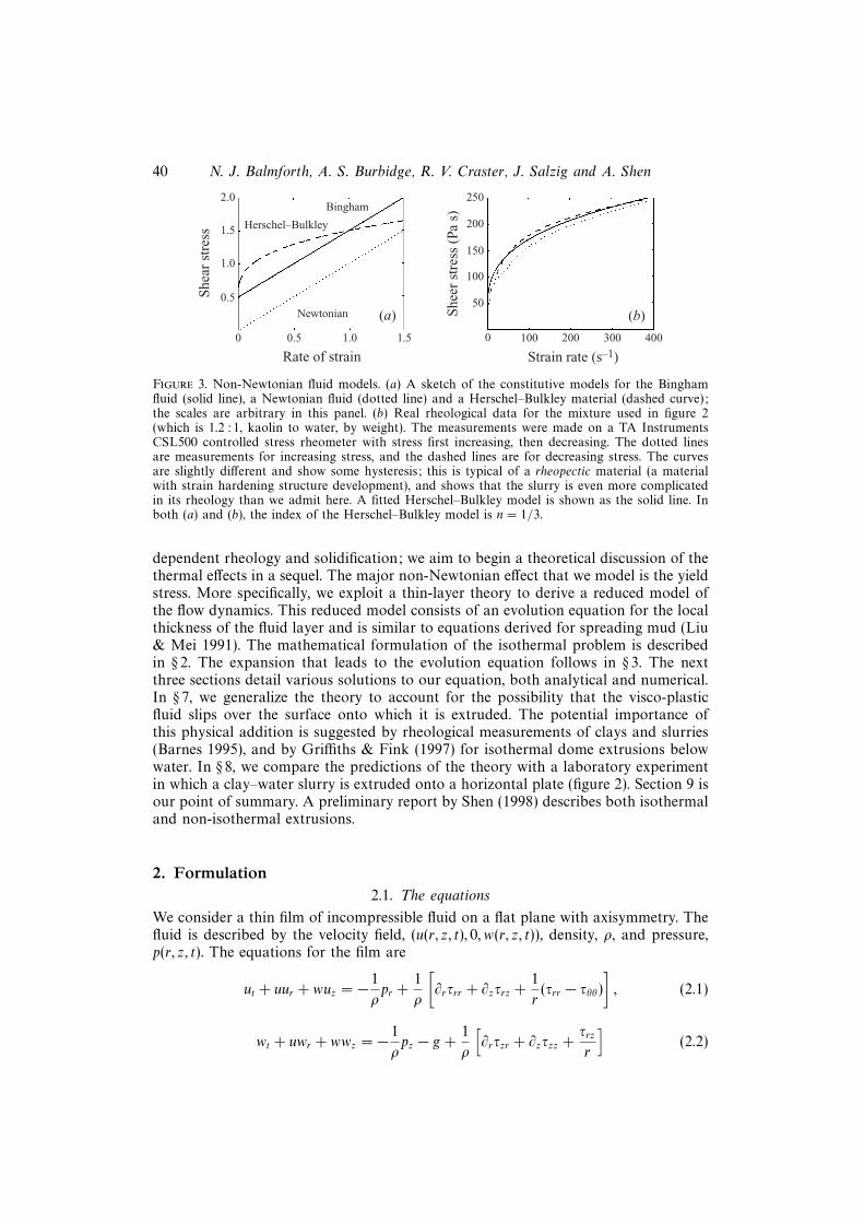
The simplest visco-plastic fluid is described by the Bingham model. This modelhas the characteristic relationship between stress and strain rate shown in figure 3:beyond a certain yield stress, the stress increases linearly with strain rate. A moreversatile non-Newtonian fluid model is the Herschel–Bulkley fluid. This model has apower-law relationship between stress and strain rate once the yield stress is exceeded(figure 3), and compares more favourably with rheological measurements of clayslurries and muds (Coussot 1994, 1997; Huang & Garcia 1998). Indeed the stress–strain-rate curves shown in Blake (1990), Hulme (1974), Griffiths & Fink (1997) allclearly have a nonlinear dependence upon the strain rate. We illustrate this featurefurther in figure 3(b), which shows the relationship between the stress and strain ratefor the mixture shown as an expanding dome in figure 2. To allow greater flexibilitywe therefore adopt the Herschel–Bulkley constitutive model.

In this paper we consider isothermal fluid flows, and so the problem does notcontain the mathematical and physical complications associated with temperature-


2.0

1.5

1.0

0.5

0 0.5 1.0 1.5

Rate of strain

(a)

She

ar s

tres

sBingham

Newtonian

Herschel–Bulkley

250

200

150

100

50

0

She

er s

tres

s (P

a s)

100 200 300 400

(b)

Strain rate (s–1)

Figure 3. Non-Newtonian fluid models. (a) A sketch of the constitutive models for the Binghamfluid (solid line), a Newtonian fluid (dotted line) and a Herschel–Bulkley material (dashed curve);the scales are arbitrary in this panel. (b) Real rheological data for the mixture used in figure 2(which is 1.2 : 1, kaolin to water, by weight). The measurements were made on a TA InstrumentsCSL500 controlled stress rheometer with stress first increasing, then decreasing. The dotted linesare measurements for increasing stress, and the dashed lines are for decreasing stress. The curvesare slightly different and show some hysteresis; this is typical of a rheopectic material (a materialwith strain hardening structure development), and shows that the slurry is even more complicatedin its rheology than we admit here. A fitted Herschel–Bulkley model is shown as the solid line. Inboth (a) and (b), the index of the Herschel–Bulkley model is n = 1/3.

dependent rheology and solidification; we aim to begin a theoretical discussion of thethermal effects in a sequel. The major non-Newtonian effect that we model is the yieldstress. More specifically, we exploit a thin-layer theory to derive a reduced model ofthe flow dynamics. This reduced model consists of an evolution equation for the localthickness of the fluid layer and is similar to equations derived for spreading mud (Liu& Mei 1991). The mathematical formulation of the isothermal problem is describedin § 2. The expansion that leads to the evolution equation follows in § 3. The nextthree sections detail various solutions to our equation, both analytical and numerical.In § 7, we generalize the theory to account for the possibility that the visco-plasticfluid slips over the surface onto which it is extruded. The potential importance ofthis physical addition is suggested by rheological measurements of clays and slurries(Barnes 1995), and by Griffiths & Fink (1997) for isothermal dome extrusions belowwater. In § 8, we compare the predictions of the theory with a laboratory experimentin which a clay–water slurry is extruded onto a horizontal plate (figure 2). Section 9 isour point of summary. A preliminary report by Shen (1998) describes both isothermaland non-isothermal extrusions.

2. Formulation2.1. The equations

We consider a thin film of incompressible fluid on a flat plane with axisymmetry. Thefluid is described by the velocity field, (u(r, z, t), 0, w(r, z, t)), density, ρ, and pressure,p(r, z, t). The equations for the film are

ut + uur + wuz = −1

ρpr +

1

ρ

[∂rτrr + ∂zτrz +

1

r(τrr − τθθ)

], (2.1)

wt + uwr + wwz = −1

ρpz − g +

1

ρ

[∂rτzr + ∂zτzz +

τrz

r

](2.2)


and1

r∂r(ru) + wz = 0, (2.3)

where the τij denote the deviatoric stresses and the symbol ∂r denotes partial differen-tial with respect to r and so forth. For a visco-plastic fluid, these stresses are relatedto the strain rates through a constitutive model; this will be discussed shortly.

We solve these equations subject to the free-surface conditions

ht + uhr = w (2.4)

and (τrr − p 0 τrz

0 τθθ − p 0τzr 0 τzz − p

)(−hr01

)=

(000

), (2.5)

on z = h(r, t).At the base we impose no slip on the velocity field, except just above the vent where

there is a source of fluid with a specified vertical velocity (we ignore the back-reactionof the dome upon the fluid moving up the vent):

u = 0 and w = ws(r, t) on z = 0. (2.6)

This boundary condition is replaced by a slip law in § 7 to study the effect of basalsliding. In all illustrative examples, the source term, ws(r, t) is taken to be of the form

ws(r, t) = w0(t)(r2∗ − r2)ϑ(r2

∗ − r2), (2.7)

where w0 depends only on t, r∗ is the vent radius and ϑ(x) indicates the step function.

2.2. Constitutive model

As we discussed in the introduction, the constitutive relation we employ is theHerschel–Bulkley model,

τij =

(Kγn−1 +

τp

γ

)γij for τ > τp (2.8)

and

γij = 0 for τ < τp (2.9)

(Oldroyd 1947; Herschel & Bulkley 1923), where γij is defined here as

γij =

(2ur 0 uz + wr0 2u/r 0

uz + wr 0 2wz

), (2.10)

that is, it is twice the rate-of-strain tensor. The second invariants of τij and γij aredefined as

τ =√

12τjkτjk and γ =

√12γjkγjk. (2.11)

The yield stress is τp, and K is the consistency. For a Bingham material, once the yieldstress is exceeded, the deviatoric stresses are directly proportional to the shear rate;thus n = 1 and K = η = ρν, where η is the plastic viscosity and ν is the kinematicviscosity. Hence, in this case, K is just conventional viscosity. In general, K provides ameasure of resistance to shear. The parameter n characterizing the nonlinearity in theflow regime determines whether the fluid is shear thinning (n < 1) or shear thickening(n > 1); lavas are almost invariably assumed to be shear thinning. However, this may


Constants Silicic lava Wax–kaolin slurry

Density, ρ (kg m−3) 2600 1320Viscosity, η (Pa s) 109 15Yield stress, τp (Pa) 105 14Index, n, 1 0.35

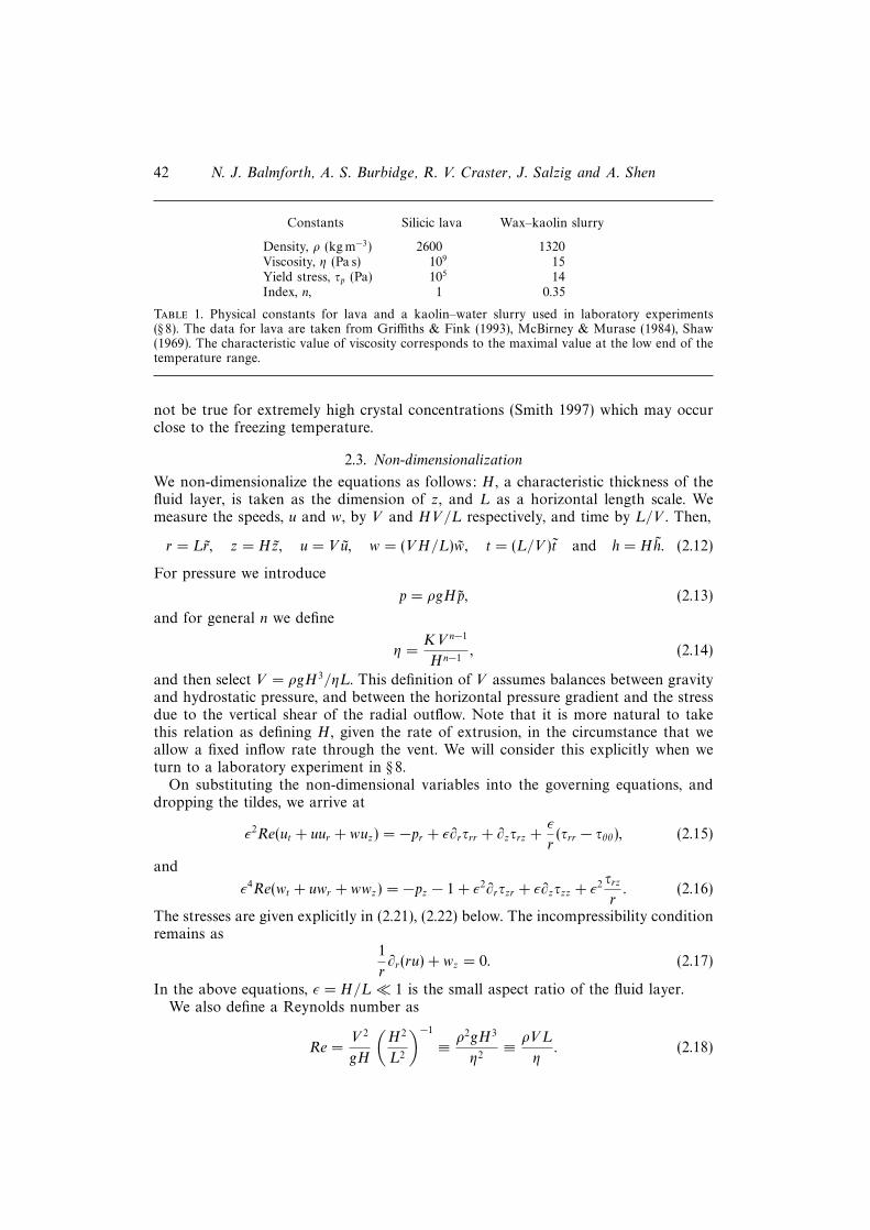
Table 1. Physical constants for lava and a kaolin–water slurry used in laboratory experiments(§ 8). The data for lava are taken from Griffiths & Fink (1993), McBirney & Murase (1984), Shaw(1969). The characteristic value of viscosity corresponds to the maximal value at the low end of thetemperature range.

not be true for extremely high crystal concentrations (Smith 1997) which may occurclose to the freezing temperature.

2.3. Non-dimensionalization

We non-dimensionalize the equations as follows: H , a characteristic thickness of thefluid layer, is taken as the dimension of z, and L as a horizontal length scale. Wemeasure the speeds, u and w, by V and HV/L respectively, and time by L/V . Then,

r = Lr, z = Hz, u = V u, w = (VH/L)w, t = (L/V )t and h = Hh. (2.12)

For pressure we introduce

p = ρgHp, (2.13)

and for general n we define

η =KVn−1

Hn−1, (2.14)

and then select V = ρgH3/ηL. This definition of V assumes balances between gravityand hydrostatic pressure, and between the horizontal pressure gradient and the stressdue to the vertical shear of the radial outflow. Note that it is more natural to takethis relation as defining H , given the rate of extrusion, in the circumstance that weallow a fixed inflow rate through the vent. We will consider this explicitly when weturn to a laboratory experiment in § 8.

On substituting the non-dimensional variables into the governing equations, anddropping the tildes, we arrive at

ε2Re(ut + uur + wuz) = −pr + ε∂rτrr + ∂zτrz +ε

r(τrr − τθθ), (2.15)

and

ε4Re(wt + uwr + wwz) = −pz − 1 + ε2∂rτzr + ε∂zτzz + ε2 τrz

r. (2.16)

The stresses are given explicitly in (2.21), (2.22) below. The incompressibility conditionremains as

1

r∂r(ru) + wz = 0. (2.17)

In the above equations, ε = H/L 1 is the small aspect ratio of the fluid layer.We also define a Reynolds number as

Re =V 2

gH

(H2

L2

)−1

≡ ρ2gH3

η2≡ ρVL

η. (2.18)


Extrusion conditions Lava Kaolin–water

Dome radius, L (m) 102 0.10Effusion rate, Q (m3 s−1) 0.1− 10 10−6

Table 2. Typical extrusion conditions for lava and kaolin–water experiments. The data for lava istaken from Griffiths & Fink (1993), McBirney & Murase (1984) and Shaw (1969).

Non-dimensional parameter Lava Kaolin–water

ε = H/L (ηQ/ρgqL4)1/4 0.1 0.01Re = ρVL/η (ρ5gQ3/η5q3)1/4 10−8 1B = τp∗H/ηV τp∗L(q/ηρgQ)1/2 1 100

Table 3. Typical values of non-dimensional numbers, given the physical constants and extrusionconditions in tables 1 and 2, assuming n = 1, q = π and Q = 1 m3 s−1 for lava. The parameterq is a non-dimensional flow rate introduced in § 8 where we relate the analysis to an experiment.(By taking q ∼ 1, we scale the problem so that the extrusion time is order unity and no furtherrescalings of time are necessary; this is unlike our numerical computations reported in § 6 in whichq ∼ 10−4 and extrusion times are long.)

We take Re to be order unity, which ensures a low Reynolds number flow, or,equivalently, the absence of inertial effects to leading orders (see table 3 for typicalvalues).

Next, with the units V/H , the components of γij become

γθθ = 2εu/r, γrr = 2εur, γrz = uz + ε2wr and γzz = 2εwz, (2.19)

and

γ =[(uz + ε2wr)

2 + 4ε2u2r + 4ε2(u/r)2

]1/2. (2.20)

Hence, in the units ρgH2/L and provided τ > B, the dimensionless stresses are givenby

τrr = 2ε

(γn−1 +

B

γ

)ur, τzz = 2ε

(γn−1 +

B

γ

)wz (2.21)

and

τθθ = 2ε

(γn−1 +

B

γ

)u/r, τrz =

(γn−1 +

B

γ

)(uz + ε2wr), (2.22)

with

τ =√τ2rz + 1

2(τ2rr + τ2

θθ + τ2zz). (2.23)

The non-dimensional group,

B =τpH

ηV≡ τpL

ρgH2, (2.24)

is a measure of the yield stress relative to the horizontal pressure gradient acting overthe thickness of the fluid; henceforth we refer to B as the Bingham number, even ifn 6= 1.

If τ < B, on the other hand, then ur = uz + ε2wr = wz = 0.The rescaled boundary conditions are

u = 0 and w = w0(t)f(r) on z = 0, (2.25)


and, on z = h(r, t),

ht + uhr = w (2.26)

and

τrz + phr = εhrτrr and p = ε(τzz − εhrτrz). (2.27)

3. The expansionWe now solve the equations by introducing an asymptotic expansion. Though there

are some subtleties in the expansion (Balmforth & Craster 1999), we actually needonly the leading-order terms of all the equations. These are

−pr + ∂zτrz = 0, (3.1)

pz = −1, (3.2)

1

r∂r(ru) + wz = 0, (3.3)

and

γ = |uz|, (3.4)

subject to

u = 0 and w = w0f(r) on z = 0 (3.5)

and

ht + uhr = w and τrz = p = 0 on z = h(r, t). (3.6)

The constitutive model is

τrz =

(γn−1 +

B

γ

)uz, for τ > B ≡ |τrz|, (3.7)

and uz = 0 if τ < B.Equation (3.2) integrates to

p = h(r, t)− z, (3.8)

and then (3.1) to

τrz = −hr(h− z). (3.9)

Evidently, τ = |hr|(h− z) decreases with z and the largest shear stress occurs alongthe base of the fluid. Here,

τ(r, 0, t) = |τrz(r, 0, t)| = |hhr|, (3.10)

which must exceed B in order for the fluid to move at all. Furthermore, at z = h,τ = 0. Hence, if the fluid is moving, the stress must fall beneath the yield stress atsome level, z = Y (r, t). This surface is given by

Y (r, t) = h− B

|hr| , (3.11)

with Y > 0 in order for the fluid to move.Below z = Y , the fluid is yielding and so

B + |uz|n−1uz = −hr(h− z), (3.12)

or

uz = [|hr|(Y − z)]1/n sgn(−hr). (3.13)


Above z = Y the fluid is rigid and uz = 0. That is, we have a ‘plug flow’. Theidentification of the plug is actually a little confusing (Lipscomb & Denn 1984) andsome clarification is required; a more detailed discussion follows equation (3.17).

Now, we define

U(r, t) =

∫ h

0

u(r, z, t) dz ≡∫ h

0

(h− z)uz(r, z, t) dz. (3.14)

Then,

U(r, t) = − n

n+ 1|hr|1/n−1Y 1+1/n

(h− nY

2n+ 1

)hrϑ(Y ), (3.15)

where ϑ(x) is the Heaviside step function. The introduction of this discontinuousfunction into U(r, t) takes care of the yield criterion, which is that, if Y < 0, the fluidis insufficiently stressed to move. In that case, the fluid as a whole is stationary andthe free surface cannot evolve (we distinguish stationary from plug flow).

The quantity U(r, t) is needed for the evolution equation for h(r, t), which we nowderive by vertically integrating the continuity equation (3.3) and using the free-surfacecondition in (3.6):

ht +1

r∂r (rU) = ws. (3.16)

The evolution equation (3.16) has a simple conservation law,

d

dt

∫ ∞0

h(r, t)r dr =

∫ ∞0

ws(r, t)r dr (3.17)

(conservation of mass), provided the only source of fluid is the vent at the origin.Note that the evolution equation models a radially expanding flow. This means that

the flow is extensional everywhere, and so there cannot be a true plug flow anywhere.This is seemingly inconsistent with the claim above that the region h > z > Ycontains a rigid plug (cf. Lipscomb & Denn 1984). In fact, what really happens isthat the leading-order solution breaks down inside this region. Further developmentsof the problem (Balmforth & Craster 1999; see also Lawrence & Corfield 1998)reveal that this region is, in fact, weakly yielding and uz ∼ O(ε). This slight yieldingis created by the conspiracy of the order-ε stress components (which includes thenormal stresses), and is sufficient to compensate the radial expansion. Importantly,the theory remains consistent. Another route out of this apparent inconsistency is touse a fluid model that does not have a real yield stress, but behaves as a very viscousfluid for small strain rates. This type of fluid model is sometimes claimed to be morerealistic than Bingham-type models (Barnes & Walters 1985), but this view is notuniformly accepted (N’Guyen & Boger 1992). Although unnecessary for analyticalwork this alternative route is convenient for numerical reasons, and we outline somedevelopments of the problem along this line in the Appendix; there we formulatethe thin-layer theory for a modified constitutive model which yields weakly at smallrates of strain. The purpose is to derive another version of our theory in which thenon-smooth functions in (3.16) become smooth.

4. Two limits in yield strengthTwo limiting cases of B are of particular importance: The power-law fluid, B → 0,

and a high yield stress fluid, B → ∞. We consider these for a constant source(ws = ws(r)).


4.1. Power-law fluid: B → 0

When B → 0, the effect of the yield stress vanishes. If n = 1, we then recover thethin-film equation for Newtonian fluid (Huppert 1982):

B = 0, n = 1: ht − 1

3r∂r(rh

3hr) = ws. (4.1)

Provided ws is a constant point source, this equation has a similarity solution,

h(r, t) = f(r/√t) ≡ f(η), (4.2)

with

− 12η2fη =

1

3

d

dη(ηf3fη), (4.3)

as found previously by Huppert (1982); see also Barenblatt (1979). Thus radius R(t)and thickness h(0, t) vary as R ∼ t1/2 and h(0, t) ∼ constant.

When n is not unity, we obtain a thin-film equation for a power-law fluid:

B = 0, n 6= 1: ht − n

(2n+ 1)r∂r(rh

2+1/nh1/nr ) = ws. (4.4)

(This is a version of the porous medium equation in radial geometry.) Again we havea similarity solution,

h(r, t) = tαf(r/tβ) = tαf(η), R(t) = R0tβ and h(0, t) = h0t

α, (4.5)

with

α =1− n3n+ 5

, β = 2

(1 + n

3n+ 5

), (4.6)

and constants, R0 and h0.

4.2. High yield stress: ‘large’ B

The opposite limit, in which the fluid is dominated by the yield stress, and B is insome sense large, is not so straightforward. As is evident from the numerical resultspresented later, this limit is characterized by solutions for which Y → 0. That is,h = h+ y, where |h| |y| for all time, and

h = −Bhr

(4.7)

(so the associated yield surface is precisely zero). This solution, and the smallness ofy must be verified from the equation satisfied by y. From (4.7) we obtain

h =

√2B(R − r), r < R

0, r > R(4.8)

where the time rate of change of the radius, R(t), is dictated by the conservation law(3.17) and the time-dependence of the source. For a constant inflow rate, Q,

R(t) =1

(2B)1/5

(15Qt

8π

)2/5

, h(0, t) = (2BR)1/2. (4.9)

This solution represents a quasi-static expansion and a steady progression throughthe equilibrium solutions found by Nye (1952); see also Blake (1990).

The scalings in (4.6) and (4.9) can also be found from dimensional analysis (Griffiths& Fink 1993) in which one assumes a balance between terms representing the pressure


gradient and basal shear stress in the governing equations. But these scalings onlyfollow in the appropriate asymptotic limits, and for general parameter values thereis no characteristic temporal dependence of height and radius of the form (4.5), asillustrated by the numerical results described shortly.

5. A similarity solution for a time-dependent sourceIf ws takes the form of a point source at r = 0, then we may look for a similarity

solution to the evolution equation (3.16) with the form

h(r, t) = tαf(r/tβ) = tαf(η). (5.1)

If ws ∼ tγ , then the conservation law (3.17) implies that

α+ 2β = γ. (5.2)

Moreover, direct substitution of (5.1) into the evolution equation gives

1

n(n+ 1)(2n+ 1)ηtβ(1+1/n)−α(1+2/n)−1(αf − βηfη)

=d

dη

[(f − nY

2n+ 1

)Y1+1/n|fη|1/n−1fη

], (5.3)

where the function Y is defined via

Y = tα[f +

B

fηtβ−2α

]+

≡ tαY, (5.4)

and where the + subscript is to remind us to take the quantity in brackets only whereit is positive, and zero otherwise. Evidently, due to the form of Y, a similarity solutionwill not in general exist. However, if β < 2α, then ultimately Y → tαf(η) and thesolution may converge to one of similarity form. In this case,

β(1 + n) = α(2 + n) + n and β < 2α. (5.5)

The conditions (5.2) and (5.5) can be rewritten in the form

α =(n+ 1)γ − 2n

3n+ 5, β =

n+ γ(n+ 2)

3n+ 5(5.6)

and γ > 5.There is a special case in which an exact similarity solution exists. This is when

γ = 5 and

h(r, t) = tf(r/t2) = tf(η), (5.7)

with

1

n(n+ 1)(2n+ 1)η(f − 2ηfη) =

d

dη

[η

(f − nY

2n+ 1

)Y1+1/n|fη|1/n−1fη

](5.8)

and Y = f + B/fη. This special case is significant also in Blake’s (1990) dimensionalanalysis. In general, however, there is no solution of similarity form for a constantsource (γ = 0). In that circumstance, the problematic term in Y does not remainsubdominant as it does if γ > 5.


6. Numerical resultsWe now describe some numerical results utilizing the thin-layer theory. The evolu-

tion equation

ht +1

r∂r(rU) = ws, (6.1)

together with equation (3.15) for U(r, t), is solved using an adaptive grid scheme; thescheme utilized is designed to solve nonlinear parabolic equations and is describedin some detail by Blom & Zegeling (1994).† We also performed some comparativesimulations using a finite element collocation scheme, PDECOL, Keast & Muir (1991).

To avoid some numerical difficulties that occur where h(r, t)→ 0, we take an initialcondition in which h(r, t) is everywhere small and finite, h(r, 0) = 10−3 exp(−r2/25),and add a linear viscous term to (6.1) with a very small coefficient (10−8). We alsoprescribe the gradient of h at the origin, and at a radius r∞ that is sufficiently largeto be considered infinite:

hr(0, t) = hr(r∞, t) = 0. (6.2)

The only remaining term to identify is the source behaviour; for this we choose

ws(r) = 0.1(r2∗ − r2)ϑ(r2

∗ − r2), (6.3)

and r∗ = 0.15, which prescribes the vent radius and flux. The value of 0.1 used for w0

has no special significance, and, in fact, a suitable scaling of r, t and B can be usedto explicitly remove this ‘free parameter’ from the problem.

Because our thin-layer equation contains some non-smooth functions, there aresome minor numerical difficulties that are circumvented by smoothing out U(r, t),as described in the Appendix. We have verified that the numerical solutions areinsensitive to the details of this regularization and the size of the parameter µ whichmeasures the degree of smoothing (see Appendix).

6.1. Bingham fluids

We first take n = 1, which corresponds to the Bingham model, and explore the effectof varying the yield stress.

In figure 4, we display results for a fluid with a very small yield stress (B = 10−5)representative of an almost Newtonian fluid. This fluid behaves essentially like aNewtonian fluid, and converges to the similarity form h(r, t) = f(r/

√t) away from

the vent (see figure 4c). Because the source has finite radius, the similarity scaling isbroken over the vent, r < r∗. Note that the extent of the source is reflected in themorphology of the dome.

A case with a relatively large yield stress is shown in figure 5; the value of B hereis 0.1 which is not actually a very large number; we enter the yield-stress-dominatedlimits at these low values of B because of our choice of dimensional units and w0 = 0.1(see table 3 and § 8). This value of B is representative of a thick paste-like material. Aswe remarked earlier, Y → 0 for the outflow. Consequently, the fluid marches slowlythrough an approximate sequence of equilibria given by Nye’s parabolic profile (4.8).The radius and height then have the scalings (4.9), as illustrated by figure 5(c).

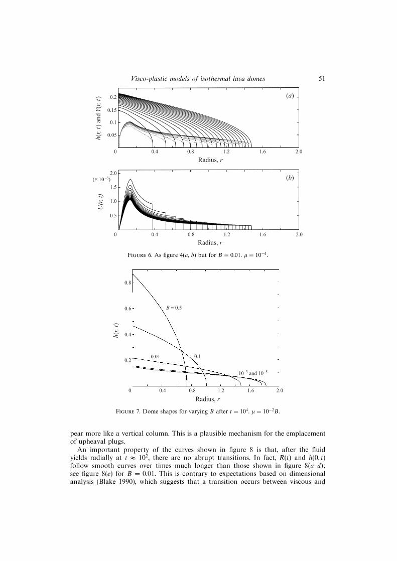
An intermediate case with moderate yield stress, B = 0.01, is shown in figure 6;this is representative of a slurry which has a substantial proportion of water. Here the‘plug’ occupies roughly half of the fluid (figure 6a), and it is not possible to collapsethe solutions in figure 6 to one of similarity form.

† The code is available at the web-site: http://www.ma.ic.ac.uk/∼rvcras/dome.f.gz.


0.15

0.10

0.05

0 0.4 0.8 1.2 1.6 2.0

Radius, r

(a)h(

r, t)

and

Y(r

, t)

(b)1.2

0.8

0.4

0 0.4 0.8 1.2 1.6 2.0

Radius, r

(c)0.15

0.10

0.05

0 0.004 0.008 0.012 0.016

g = r /t1/2

t0 h(

r, t)

U(r

, t)

(× 10–4)

Figure 4. Evolution for B = 10−5. (a) The height field, h(r, t), together with the ‘yield’ surface, Y (r, t)shown by the dotted lines. The yield surface is everywhere indistinguishable from the height exceptin a slender region around the origin. (b) U(r, t), the vertical integral of u(r, z, t). (c) The height fieldis plotted against the similarity coordinate η = r/t1/2. Shown are snapshots of the solution every500 time units. The regularization parameter of the Appendix is µ = 10−7.

A selection of dome shapes is shown in figure 7. This figure shows the height, h(r, t),at t = 104 for various computations using different B. As the yield stress increases,the aspect ratio of the dome increases and the shape becomes increasingly parabolic.‡Note that for the larger values of B, the dome appears to have a finite gradient atr = 0, hr(0, t) 6= 0, in violation of the symmetry condition imposed there. The reasonfor this is that if hr → 0, then Y (0, t) = 0 and the central portion of the fluid neveryields. But if Y → 0, then the fluid at the centre of the dome cannot flow radially;instead we have the balance ht = ws, which implies a continual build-up of the domecentre. But such a fluid structure must yield sideways. The fluid finds its way out ofthis conundrum by building up the gradient of h(r, t) in an increasingly narrow regionaround r = 0. However, over the region with r = O(ε), the thin-layer theory breaks

‡ The pictures are all displayed in dimensionless units. This means that εh(0, t)/R(t) is the actualaspect ratio, which is much smaller (by the factor of ε) than the figures appear to suggest.


0.5

0.4

0.3

0 0.4 0.8 1.2 1.6 2.0

Radius, r

(a)h(

r, t)

and

Y(r

, t)

(b)1.0

0.8

0.6

0 0.4 0.8 1.2 1.6 2.0

Radius, r

(c)0.06

0.04

0.02

0 0.005 0.010 0.015 0.025

g = r /t2/5

t–1/5

h(r

, t)

U(r

, t)

(× 10–3)

0.2

0.1

0.4

0.2

0.020

Figure 5. As figure 4 but for B = 0.1. In (c), the height field is scaled by t1/5 and plotted againstthe similarity coordinate η = r/t2/5. µ = 10−4.

down and we should strictly use a different asymptotic expansion (cf. Johnson 1984).We assume that the global structure of the dome is insensitive to this slight deficiencyin the model.

In figure 8 we show radius and height evolution for five values of B. (For computa-tional convenience, we define the radius R(t) as the location for which h(R, t) = 0.01.)This shows the convergence to a scaling somewhere between the Newtonian anddominating yield-stress limits. One other feature brought out in this figure is thelinear-in-time increase in the height field for small times. This stage of the domegrowth involves the predominantly vertical rise of the fluid out of the vent: the fluidinitially rises up like extruded toothpaste and does not yield radially. Eventually (anddepending on the size of B), the extruded fluid yields under its own weight and flowsradially (as shown in figure 9); similar behaviour has been noted in the flows ofpastes (Burbidge & Bridgwater 1999) and observed in the experiments of Griffiths &Fink (1997). If the extrusion of fluid from the vent were abruptly to cease whilst theexpansion was still in this phase, and solidification then to ensue, the dome would ap-


0.2

0.15

0.1

0.05

0 0.4 0.8 1.2 1.6 2.0

(a)

(b)

Radius, r

2.0

1.5

1.0

0.5

0 0.4 0.8 1.2 1.6 2.0

Radius, r

(× 10–3)

U(r

, t)

h(r,

t) a

nd Y

(r, t

)

Figure 6. As figure 4(a, b) but for B = 0.01. µ = 10−4.

0.8

0.6

0.4

0.2

0 0.4 0.8 1.2 1.6 2.0

B = 0.5

0.01 0.1

10–3 and 10–5

Radius, r

h(r,

t)

Figure 7. Dome shapes for varying B after t = 104. µ = 10−2B.

pear more like a vertical column. This is a plausible mechanism for the emplacementof upheaval plugs.

An important property of the curves shown in figure 8 is that, after the fluidyields radially at t ≈ 102, there are no abrupt transitions. In fact, R(t) and h(0, t)follow smooth curves over times much longer than those shown in figure 8(a–d);see figure 8(e) for B = 0.01. This is contrary to expectations based on dimensionalanalysis (Blake 1990), which suggests that a transition occurs between viscous and


B = 10–4

B = 0.5

1/2

2/5

100

10–1

101 102 103 104

t

R(t

)

(a) 100

10–1

101 102 103 104

t

h(0,

t)

(b) 1/5

1

0

100

10–1

10–1 100

R(t)

h(0,

t)

(c)1/2

0

(d )

Yield point

0

0.25

0.20

0.15

0.10

0.05

t50 100 150 200 250

R(t

) an

d h(

0, t)

101

100

10–1

102 103 104 105 106

(e)

R(t

) an

d h(

0, t)

Time

R(t)

h(0, t)

Figure 8. The variation in the radius and height with time for various values of B (10−4, 10−3, 10−2,0.1 and 0.5. (a) R(t) and (b) h(0, t). (c) h(0, t) plotted against R(t) and (d) the early development forthe particular case B = 0.1; the solid line is R(t) and the dashed line is h(0, t). Characteristic scalingsfor the Newtonian and yield-stress-dominated cases are also shown by the dotted lines and stars.(e) R(t) (solid line) and h(0, t) (dashed line) over a longer timescale; the dotted lines again show theviscous and yield-stress-dominated scalings. µ = 10−2B.

yield-stress-dominated dynamics at a time

tB =q1/4

B2, (6.4)

in dimensionless units, where q = πr4∗w0/2 is the dimensionless effusion rate. Forexample, tB = 944 for B = 0.01, but no transition occurs for such times in fig-ure 8(e). The dimensional analysis assumes a switch between dominant behavioursbut, evidently, the dome chooses a more balanced path between the two extremes.

6.2. Variations with power-law index

The clarity of this picture of the dynamics of lava-dome expansion is obscured whenwe allow n to vary; once the fluid flows it now follows a nonlinear stress–strain-raterelation and the resulting dynamical changes can compete with or complement theeffect of yield stress. Note that experiments invariably have n < 1, corresponding toshear thinning; physically this models the destruction of the internal structure of the


0.25

0.20

0.10

0 0.05 0.10 0.15 0.20

Vent radius

Radius, r

h(r,

t)0.05

0.15

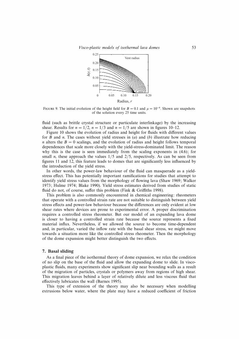
Figure 9. The initial evolution of the height field for B = 0.1 and µ = 10−4. Shown are snapshotsof the solution every 25 time units.

fluid (such as brittle crystal structure or particulate interlinkage) by the increasingshear. Results for n = 1/2, n = 1/3 and n = 1/5 are shown in figures 10–12.

Figure 10 shows the evolution of radius and height for fluids with different valuesfor B and n. The cases without yield stresses in (a) and (b) illustrate how reducingn alters the B = 0 scalings, and the evolution of radius and height follows temporaldependences that scale more closely with the yield-stress-dominated limit. The reasonwhy this is the case is seen immediately from the scaling exponents in (4.6); forsmall n, these approach the values 1/5 and 2/5, respectively. As can be seen fromfigures 11 and 12, this feature leads to domes that are significantly less influenced bythe introduction of the yield stress.

In other words, the power-law behaviour of the fluid can masquerade as a yield-stress effect. This has potentially important ramifications for studies that attempt toidentify yield stress values from the morphology of flowing lava (Shaw 1969; Walker1973; Hulme 1974; Blake 1990). Yield stress estimates derived from studies of staticfluid do not, of course, suffer this problem (Fink & Griffiths 1998).

This problem is also commonly encountered in chemical engineering: rheometersthat operate with a controlled strain rate are not suitable to distinguish between yieldstress effects and power-law behaviour because the differences are only evident at lowshear rates where devices are prone to experimental error. A proper discriminationrequires a controlled stress rheometer. But our model of an expanding lava domeis closer to having a controlled strain rate because the source represents a fixedmaterial influx. Nevertheless, if we allowed the source to become time-dependentand, in particular, varied the inflow rate with the basal shear stress, we might movetowards a situation more like the controlled stress rheometer. Then the morphologyof the dome expansion might better distinguish the two effects.

7. Basal slidingAs a final piece of the isothermal theory of dome expansion, we relax the condition

of no slip on the base of the fluid and allow the expanding dome to slide. In visco-plastic fluids, many experiments show significant slip near bounding walls as a resultof the migration of particles, crystals or polymers away from regions of high shear.This migration leaves behind a layer of relatively dilute and less viscous fluid thateffectively lubricates the wall (Barnes 1995).

This type of extension of the theory may also be necessary when modellingextrusions below water, where the plate may have a reduced coefficient of friction


(a) (d)

(b) (e)

(c) ( f )

100

10–1

101 102 103 104

t

R(t

)

10–1

102 103 104

h(0,

t)

100

10–1

101 102 103 104

t

R(t

)

10–1

102 103 104

h(0,

t)

100

10–1

101 102 103 104

t

R(t

)

10–1

102 103 104

h(0,

t)

B = 0, n = 1

B = 0

B = 0.01

B = 0.1

t

t

t

Figure 10. Evolution of radius and dome height for various values of B and n: (a, d) n = 1/2,(b, e) n = 1/3, (c, f) n = 1/5. µ = 10−2B.

0.5

0.4

0.3

0.2

0.1

0 0.4 0.8 1.2 1.6 2.0

Radius, r

Hei

ght h

(r, t

)

Figure 11. Evolution for B = 0 and n = 1/3. Shown is the height field, h(r, t), every 500 time units.


0.6

0.5

0.4

0.3

0.2

0.1

0 0.4 0.8 1.2 1.6 2.0

Radius, r

Hei

ght,

h(r,

t)n = 1/5n = 1/3

n = 1/2

B = 0B = 0.01B = 0, n = 1

Figure 12. Dome shapes for varying B and n after t = 104. µ = 10−2B.

(Griffiths & Fink 1997); such experiments are typical in non-isothermal studies(Hallworth et al. 1987). Moreover, in real lavas (and in glaciers), motion over a roughbase can take place through a succession of solidification and melting. This processcan produce an effective slip (Hutter 1983).

In many engineering contexts, the no-slip condition is replaced by some empiricallaw relating the stress at the wall to the sliding velocity. Here we adopt the relation,

|τrz| = Bw + p0Ω(p0)uαb if |τrz| > Bw,

ub = 0 if |τrz| < Bw(7.1)

in dimensionless notation, where p0 = p(r, z = 0, t) is the pressure at the base of thefluid, ub is the radial sliding speed, and Bw = τwH/ηU is a Bingham number thatmeasures a yield stress at the base (so the fluid only slips if the stress exceeds acertain threshold, τw). Also, α is some power-law index and the arbitrary functionΩ(p0) allows for a nonlinear friction law. Equation (7.1) is a version of Mooney’slaw (Mooney 1931). Without the basal yield stress, boundary conditions of this kindare used in glaciology (Hutter 1983; Fowler 1989; Morland 1997) and for flows ofconcentrated suspensions (Benbow & Bridgwater 1993).

We may now proceed with the asymptotic expansion once again. The calculationis little different; manipulations like those used earlier lead to

U(r, t) =

∫ h

0

(h− z)uz(r, z, t) dz

= − n

n+ 1|hr|1/n−1Y 1+1/n

(h− nY

2n+ 1

)hrϑ(Y ). (7.2)

However, U(r, t) is no longer the vertical average of the radial outflow speed. Rather,

U(r, t) =

∫ h

0

u(r, z, t)− hub. (7.3)


Moreover, from our sliding law,

ub =

[−hrYwhΩ(h)

]1/α

, (7.4)

where

Yw =

(h− Bw

|hr|)

+

. (7.5)

This minor modification introduces a new term into the evolution equation, whichis now

ht +1

r∂r[r(U + hub)] = ws. (7.6)

Note that, if Bw < B (for pastes Bw is typically 10–30% of B), the fluid layer can beinsufficiently stressed to shear internally, but it may still slide if Yw > 0. Again, thereis a conceptual difficulty with this interpretation of the radial expansion: the fluidcannot be truly unyielding, but is order ε above the yield stress.

We illustrate the effects of sliding on the character of the dome expansion bychoosing Ω(h) = constant, α = 1 and Bw = 0. Then ub = −hr/Ω. Some numericalresults for this case are illustrated in figure 13.

Evidently, the slip of the fluid breaks the characteristic temporal scalings of radiusand height for the yield-stress-dominated limit, which would otherwise be found forthe particular case shown in figure 13 (B = 0.1). Instead, there is no longer a similarityscaling for the slipping dome. Note that sliding also changes the shape of the domenear its edge, and, in particular, produces a characteristic ‘skirt’. This feature mightbe useful in empirically estimating the degree of sliding simply from the dome shape.

In fact, a difference in the temporal scalings of radius and height was previouslynoted by Griffiths & Fink (1997) between isothermal extrusions in air and belowwater. They found that domes below water were significantly lower than dry domes,a feature that is naturally explained in terms of basal slip. However, the experimentaldomes also showed little tendency to form a leading ‘skirt’. Perhaps the fracturingprocess mentioned by Griffiths & Fink offers a better explanation of the differingexperimental scalings than basal slip.

8. Experimental resultsTo provide a laboratory comparison with the theoretical results we conducted

experiments with kaolin–water slurry; these are similar to Hulme (1974) and Blake(1990). In particular, we extruded slurries in the fashion illustrated in figure 2. Weperformed two sets of experiments with two quite different experimental configura-tions: one is described by Shen (1998), and the results of a particular experiment withthe other set-up are reported here (the extrusions showed no essential differences inthe two cases).

8.1. Restoring the dimensions

To compare theory and observation, we must first restore the dimensions in ournumerical solutions. To do this we need to estimate the length scales, L and H , andthe characteristic velocity, V .

To fix the horizontal length scale we match the dimensional vent radius, Lr∗ ≡0.15L, with the size of the opening in the experimental apparatus: R∗ ≈ 1.5 mm. ThusL = 1 cm.


0.4

0.3

0.2

0.1

0 0.4 0.8 1.2 1.6 2.0

(a)

Radius, r

h(r,

t) a

nd Y

(r, t

)

(b) (c)100

10–1

010–3

10–4

5 × 10–4

101 102 103 104

Time, t

10–1

101 102 103 104

Time, t

h(0,

t)

R( t

)

(d )

0.5

0.4

0.3

0.2

0.1

0 0.5 1.0 1.5 2.0 2.5 3.0

10–3

0 and 10–5

Radius, r

Hei

ght,

h(r,

t)

Figure 13. Evolution for a dome with basal sliding. B = 0.1 and µ = 10−4. (a) The height field every500 time units for Ω = 104. (b, c) The evolution of the dome radius and height for models withΩ−1 = 10−3, 5× 10−4, 10−4 and 0. (d) Dome shapes at t = 104 for Ω−1 = 10−3, 5× 10−4, 2× 10−4,10−4, 10−5, and 0.

We also have the dimensionless flow rate (obtained by integrating the source termover the vent),

q = 12πr4∗w0, (8.1)

in which we select w0 = 0.1, as in § 7. In dimensional units, the volume flux is

Q = LHVq. (8.2)


But we also have the relation

V =ρgH3

ηLor Vn =

ρgH2+n

KL, (8.3)

since η = KVn−1/Hn−1. Thus, on eliminating V :

H =

(KL1−nQn

ρgqn

)1/(2n+2)

. (8.4)

This allows us to compute H and V given Q and L. Hence we may reconstruct thedimensional radius, height and time. Finally we estimate B:

B =τpH

ηV≡ τp

(L2nqn

ρngnKQn

)1/(n+1)

. (8.5)

The definitions above amount to evaluating ε = H/L and B in terms of theexperimental parameters. In fact, we could have based our non-dimensionalization of§ 2.3 on these parameters, and couched the formalism accordingly. One consequenceof our current non-dimensionalization is that the velocity scale is given by balancingthe viscous shear stress against the hydrostatic pressure gradient. But in yield-stress-dominated fluids, it would be preferable to balance that gradient against the yieldstress.

Also, in our numerical experiments, q = πr4∗w0/2 ∼ 10−4. It is this relatively smallnon-dimensional effusion rate that leads to the deceptively low value of B at whichwe enter the yield-stress-dominated regime.

Nevertheless, § 2.3 follows the standard routes of lubrication analysis in Newtonianand non-Newtonian fluid mechanics, and for this reason we have elected to delay thereformulation in terms of the experimental parameters until now.

8.2. Comparison of theory and experiment

We compare theory and experiment in figure 14. The particular experiment is con-ducted with a slurry of density ρ = 1.32 g cm−3, and for which we fit the rheology witha Herschel–Bulkley model with parameters, τp = 14 Pa, K = 15 (Pa s)n, and n = 0.35.The flow rate is 8.445× 10−2 cm3 s−1.

With the relevant dimensional scalings, we calculate the Bingham number asB = 0.0875. This indicates that the dome is close to the yield-stress-dominated limit.However, as also indicated in the figure, there is certainly some difference between thepredictions of the thin-layer equation and Nye’s asymptotic solution given in § 4.2. Inany case, theory and experiment show reassuring agreement.

9. ConclusionIn this study we have presented a theory with which we can analyse isothermal

lava flow. In particular, with the thin-film evolution equation, we may attempt to pickapart the physical ingredients in the problem. In this way we hope to separate effectssuch as viscosity, yield stress, shear thinning and basal sliding, and identify whichcould be most important in real lava domes. Within the limitations of the theory here,we identify the values of B for which we enter the yield-stress-dominated limit; forreal lava domes the values of B are close to that regime suggesting that yield stressesare indeed important.


50

40

30

20

10

100 200 300 400 500

Time (s)

(a)

(b)12

10

8

6

4100 200 300 400 500

Time (s)

Hei

ght (

mm

)R

adiu

s (m

m)

Figure 14. Experimental and theoretical comparison of dome evolution. (a) The radius: threemeasurements shown by dotted lines (part of the difference in the three curves is due to the factthat the dome was not precisely axisymmetrical, but showed slight asymmetry), that are averagedto compute the solid line. The dashed line is the analogous theoretical curve from solving the thinlayer equation, and the dot-dashed line is that for Nye’s asymptotic solution. (b) Comparison ofheight measurements, but there is only a single experimental curve (the solid line).

The results agree with the laboratory experiments that we have also conducted.This gives us extra motivation to continue on to the non-isothermal problem that wewill describe in future work.

We should, however, warn the reader of some deficiencies in the thin-layer theory.One drawback of the asymptotic reduction of the problem has already appeared inthe discussion of numerical results: the expansion must surely fail close to the centreof the dome, and the physical significance of solutions that appear to develop radialgradients near r = 0 is questionable. A similar breakdown of the asymptotic theoryarises where h→ 0. We have tacitly avoided a discussion of this contact ring here bytaking initial conditions in which fluid was present everywhere. But we could explicitlyconsider the contact ring in more detail, much as has been done in a variety of studiesof spreading of liquid drops (Greenspan 1978; Ehrhard & Davis 1991; Ehrhard 1993).This entails a more involved discussion of the dynamics of the contact ring and drawsin more physics. Notably, as the asymptotic expansion is currently set out, the theory


must break down in order for the dome to expand: the no-slip condition rules outexpansion without some kind of local overturning of the fluid surface at the domeedge. It is typical to avoid this inconsistency by allowing for some slip of the contactring (Dussan V. 1979); basically, the no-slip condition is relaxed using a slip law likethat described in § 7.

One might also argue that if the extrusion takes place on a surface that is notperfectly horizontal, then the dome will slump to one side, and we will lose theaxisymmetry that underlies the theory. Indeed, Fink & Griffiths (1992) and Coussot,Proust & Ancey (1996) display experiments in which just this effect was studiedexperimentally. However, whereas many geophysical settings for lava domes will notbe horizontal, there are many examples of domes that are nearly axisymmetric, sug-gesting that the slumping is not important (see figure 1). Moreover, in the laboratory,we may engineer the plate to be as horizontal as desired. Thus we do not considerdesymmetrizing effects to be especially important. Nevertheless, provided the slope isnot too steep (the angle made between the plate and the horizontal is order ε or less),we can easily add the effects of the slope into the thin-layer theory; the equationsbecome two-dimensional and the slope enters as a symmetry-breaking term. Theextension of the theory follows that for flows on planes by Balmforth & Craster(1999).

Finally, we mention that the numerical computations presented here have exclu-sively dealt with the case of a constant source. It is largely as a result of thisprescription that we have difficulty in distinguishing power-law behaviour from theyield stress. However, we need not prescribe w0(t) in this way, and there may be bettersource functions that facilitate a discrimination of the two effects. Such modificationsto our model may guide future experiments.

But there are also geophysical motivations for allowing the source to be time-dependent. For example, the lava flow probably begins as the upcoming fluid forcesits way through the overlying rocks and gradually opens a vent. Thus, initially, theflow rate slowly increases. Moreover, extrusions may be of limited duration if theoutflowing magma is of finite volume, or if the vent ultimately closes due to thereduction in subterranean pressure caused by the outflow and the solidification of thelava. The pressure of the expanding dome may also react back on the fluid movingup the vent, leading to a dynamical control of the source (Stasiuk & Jaupart 1997).In other words, the mechanics of the source can be a complicated, time-dependentprocess. Indeed, there is geophysical evidence that dome growth can take placethrough a sequence of distinct extrusions rather than a long continuous affair (forexample, in the case of Mount St. Helens, it is estimated that about fifteen distinctepisodes created the dome; Swanson & Holcomb 1989). But whatever is neededfor the additional physical input to the problem, the theory can be easily extendedby simply modifying the source function, ws(r, t); our evolution equation remains aconcise description of the expanding dome.

We thank both R. Griffiths and J. Fink for constructive criticisms of the manuscript,and a referee for drawing our attention to some useful references. The financial supportof an EPSRC Advanced Fellowship is gratefully acknowledged by R. V. C. This workwas done partly during the 1998 Geophysical Fluid Dynamics summer study program,Woods Hole Oceanographic Institution. N. J. B. was partially supported by the NSFGrant OCE-9616017 and an EPSRC Visiting Fellowship Grant GR/M50409, andthanks the ISI Foundation, Torino, and Imperial College, London, for hospitalityduring part of this work.


2.5

2.0

1.5

1.0

0.5

0 0.5 1.0 1.5Shear rate

She

ar s

tres

s

Bingham

Modified model

Figure 15. Constitutive models for the Bingham fluid and its regularization according to (A 1); thescales are arbitrary in this figure.

Appendix. RegularizationNumerical investigations utilizing the Bingham and Herschel–Bulkley models are

complicated by the presence of the discontinuity in the derivative of the stress–strain-rate relation (there is no obstacle to careful analytical study). There are severalavenues that can ease the numerical simulations. We adopt a route that has somephysical basis, and regularize the constitutive model by, in effect, smoothing outthe discontinuity. In the non-dimensional units of the main text, we regularize byadopting the new constitutive law,

τij =

(|γ|n−1 +

B√µ2 + γ2

)γ. (A 1)

The parameter µ modifies the constitutive model as indicated in figure 15; the fluidbecomes weakly yielding at low strain rates, as is suggested by experiments with manyreal non-Newtonian materials (Barnes & Walters 1985). There are many possibleforms for the modified model; equation (A 1) has no special significance among allthese possibilities. Provided µ is small, the form of the modification is not important;we use (A 1) essentially only as a numerical device that ultimately smooths out thefunction U(r, t) of the main discussion. We describe this in detail for the Binghamfluid, and generalize the formulae to general n at the end of this Appendix.

In the thin-layer theory, the leading-order non-dimensional equations are sum-marized as

pr = ∂zτrz and pz = −1. (A 2)

With the stress-free boundary condition, these may be integrated to

p = h− z and τrz = −hr(h− z). (A 3)

The constitutive model, on the other hand, leads to

τrz = uz

(1 +

B√µ2 + u2

z

), (A 4)

for n = 1. This is a quartic equation for uz . To generate the evolution equation weneed to solve (A 4), and then integrate the product of the result with h − z in orderto provide the vertical integral of u. We will not, however, do this explicitly.

For a flow of uniform depth some solutions of the quartic are displayed in


1.0

0.8

0.6

0.4

0.2

00 0.2 0.4 0.6 0.8 1.0

z

uz

(a) (b)1.0

0.8

0.6

0.4

0.2

0 0.1 0.2 0.3 0.4

u

z

Pseudo-plugFake yield surface

Fully plastic flow

l = 10–4, 10–3, 10–2, 0.1

Figure 16. Sketches of the vertical profiles of (a) the velocity gradient, uz , and (b) u for differentvalues of µ.

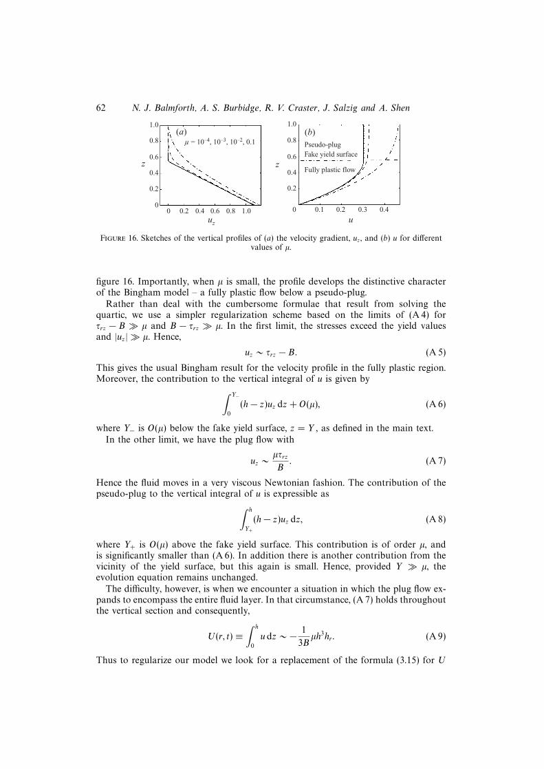
figure 16. Importantly, when µ is small, the profile develops the distinctive characterof the Bingham model – a fully plastic flow below a pseudo-plug.

Rather than deal with the cumbersome formulae that result from solving thequartic, we use a simpler regularization scheme based on the limits of (A 4) forτrz − B µ and B − τrz µ. In the first limit, the stresses exceed the yield valuesand |uz| µ. Hence,

uz ∼ τrz − B. (A 5)

This gives the usual Bingham result for the velocity profile in the fully plastic region.Moreover, the contribution to the vertical integral of u is given by∫ Y−

0

(h− z)uz dz + O(µ), (A 6)

where Y− is O(µ) below the fake yield surface, z = Y , as defined in the main text.In the other limit, we have the plug flow with

uz ∼ µτrz

B. (A 7)

Hence the fluid moves in a very viscous Newtonian fashion. The contribution of thepseudo-plug to the vertical integral of u is expressible as∫ h

Y+

(h− z)uz dz, (A 8)

where Y+ is O(µ) above the fake yield surface. This contribution is of order µ, andis significantly smaller than (A 6). In addition there is another contribution from thevicinity of the yield surface, but this again is small. Hence, provided Y µ, theevolution equation remains unchanged.

The difficulty, however, is when we encounter a situation in which the plug flow ex-pands to encompass the entire fluid layer. In that circumstance, (A 7) holds throughoutthe vertical section and consequently,

U(r, t) ≡∫ h

0

u dz ∼ − 1

3Bµh3hr. (A 9)

Thus to regularize our model we look for a replacement of the formula (3.15) for U


0.10

0.08

0.06

0.04

0.02

0–0.2 0 0.2 0.4

s* – B

F(s

* – B

)(a)

10–5

10–10

(b)

–0.2 0 0.2 0.4

Figure 17. Comparison of exact and approximate regularizations for µ = 10−4 and B = 0.5.(a)

∫ τ∗0γτ dτ, where τ∗ = −hhr , and the result in (A 10), divided by h2

r , against τ∗ − B. In (b)any differences are amplified by using logarithmic scalings. The dashed line is the exact result(numerically integrated), and the solid curve is our approximation. The errors for τ∗ < B areinconsequential since the vertical integral of u is very small there.

which limits to a small, Newtonian-like form such as (A 9). In particular, we select

U(r, t) ≈ − 1

24(3h− Y )

[Y +

√Y 2 +

µh3/2

B|hr|1/2]2

hr. (A 10)

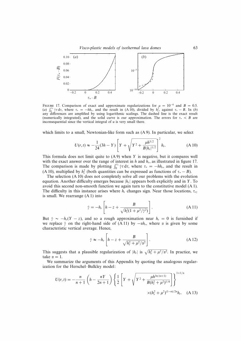
This formula does not limit quite to (A 9) when Y is negative, but it compares wellwith the exact answer over the range of interest in h and hr , as illustrated in figure 17.The comparison is made by plotting

∫ τ∗0γτ dτ, where τ∗ = −hhr , and the result in

(A 10), multiplied by h2r (both quantities can be expressed as functions of τ∗ − B).

The selection (A 10) does not completely solve all our problems with the evolutionequation. Another difficulty emerges because |hr| appears both explicitly and in Y . Toavoid this second non-smooth function we again turn to the constitutive model (A 1).The difficulty in this instance arises where hr changes sign. Near those locations, τrzis small. We rearrange (A 1) into

γ = −hr[h− z +

B√h2r (1 + µ2/γ2)

]. (A 11)

But γ ∼ −hr(Y − z), and so a rough approximation near hr = 0 is furnished ifwe replace γ on the right-hand side of (A 11) by −αhr , where α is given by somecharacteristic vertical average. Hence,

γ ≈ −hr[h− z +

B√h2r + µ2/α2

]. (A 12)

This suggests that a plausible regularization of |hr| is√h2r + µ2/α2. In practice, we

take α = 1.We summarize the arguments of this Appendix by quoting the analogous regular-

ization for the Herschel–Bulkley model:

U(r, t) = − n

n+ 1

(h− nY

2n+ 1

)1

2

[Y +

√Y 2 +

µh3n/(n+1)

B(h2r + µ2)1/4

]1+1/n

×(h2r + µ2)(1−n)/2nhr. (A 13)


This formula smooths out all the problematic terms in the evolution equation; weneed only take µ B (and verify that the results are not dependent on the details ofthe regularization, which we indeed find to be the case).

REFERENCES

Balmforth, N. J. & Craster, R. V. 1999 A consistent thin-layer theory for Bingham fluids.J. Non-Newtonian Fluid Mech. 84, 65–81.

Barenblatt, G. I. 1979 Similarity, Self-Similarity, and Intermediate Asymptotics . New York: Con-sultants Bureau.

Barnes, H. A. 1995 A review of the slip (wall depletion) of polymer solutions, emulsions andparticle slip in viscometers – its cause, character, and cure. J. Non-Newtonian Fluid Mech. 56,221–251.

Barnes, H. A. & Walters, K. 1985 The yield stress myth? Rheol. Acta 24, 323–326.

Benbow, J. J. & Bridgwater, J. 1993 Paste Flow and Extrusion . Clarendon.

Blake, S. 1990 Viscoplastic models of lava domes. In Lava Flows and Domes: EmplacementMechanisms and Hazard Implications (ed. J. H. Fink), pp. 88–128. IAVCEI Proc. Volcanology,vol. 2. Springer.

Blom, J. G. & Zegeling, P. A. 1994 Algorithm 731: a moving-grid interface for systems of one-dimensional time-dependent partial differential equations. ACM Trans. Math. Software 20,194–214.

Burbidge, A. S. & Bridgwater, J. 1999 Unsteady state planar divergent flow of extrusion pastes.Powder Technology (to appear).

Coussot, P. 1994 Steady laminar flow of concentrated mud suspensions in open channels. J. Hydr.Res. 32, 535–550.

Coussot, P. 1997 Mudflow Rheology and Dynamics . IAHR Monograph Series, Balkema.

Coussot, P., Proust, S. & Ancey, C. 1996 Rheological interpretation of deposits of yield stressfluids. J. Non-Newtonian Fluid Mech. 66, 55–70.

Davies, T. R. H. 1986 Large debris flows: a macro-viscous phenomenon. Acta Mechanica 63,161–178.

Dent, J. P. & Lang, T. E. 1983 A biviscous modified Bingham model of snow avalanche motion.Ann. Glaciology 4, 42–46.

Dussan V., E. B. 1979 On the spreading of liquids on solid surfaces: static and dynamic contactlines. Ann. Rev. Fluid Mech. 11, 371–400.

Ehrhard, P. 1993 Experiments on isothermal and non-isothermal spreading. J. Fluid Mech. 257,463–483.

Ehrhard, P. & Davis, S. H. 1991 Non-isothermal spreading of liquid drops on horizontal plates.J. Fluid Mech. 220, 365–388.

Fink, J. H. & Griffiths, R. W. 1992 A laboratory study of the surface morphology of lava flowsextruded from point and line sources. J. Volcan. Geotherm. Res. 54, 19–32.

Fink, J. H. & Griffiths, R. W. 1998 Morphology, eruption rates and rheology of lava domes:insights from laboratory models. J. Geophys. Res. 103, 527–545.

Fowler, A. C. 1989 A mathematical analysis of glacier surges. SIAM J. Appl. Maths 49, 246–263.

Fowler, A. C. 1992 Modelling ice sheet dynamics. Geophys. Astrophys. Fluid Dyn. 63, 29–65.

Greenspan, H. P. 1978 On the motion of a small viscous droplet that wets a surface. J. Fluid Mech.84, 125–143.

Griffiths, R. W. & Fink, J. H. 1993 Effects of surface cooling on the spreading of lava flows anddomes. J. Fluid Mech. 252, 667–702.

Griffiths, R. W. & Fink, J. H. 1997 Solidifying Bingham extrusions: A model for the growth ofsilicic lava domes. J. Fluid Mech. 347, 13–36.

Hallworth, M. A., Huppert, H. E. & Sparks, R. S. J. 1987 A laboratory simulation of basalticlava flows. Modern Geol. 11, 93–107.

Herschel, W. H. & Bulkley, R. 1923 Uber die viskositat und Elastizitat von Solen. Am. Soc.Testing Mater. 26, 621–633.

Huang, X. & Garcia, M. H. 1998 A Herschel–Bulkley model for mud flow down a slope. J. FluidMech. 374, 305–333.


Hulme, G. 1974 The interpretation of lava flow morphology. Geophys. J. R. Astron. Soc. 39,361–383.

Huppert, H. E. 1982 The propagation of two-dimensional and axisymmetric viscous gravity currentsover a rigid horizontal surface. J. Fluid Mech. 121, 43–58.

Hutter, K. 1983 Theoretical Glaciology . D. Reidel.

Johnson, R. E. 1984 Power-law creep of a material being compressed between parallel plates: asingular perturbation problem. J. Engng Maths 18, 105–117.

Keast, P. & Muir, P. H. 1991 Algorithm 688 EPDCOL – a more efficient PDECOL code. ACMTrans. Math. Software 17, 153–166.

Lawrence, C. J. & Corfield, G. M. 1998 Non-viscometric flow of viscoplastic materials: squeezeflow. In Dynamics of Complex Fluids (ed. M. J. Adams, R. A. Mashelkar, J. R. A. Pearson &A. R. Rennie), pp. 379–393. Imperial College Press/The Royal Society.

Lipscomb, G. G. & Denn, M. M. 1984 Flow of Bingham fluids in complex geometries.J. Non-Newtonian Fluid Mech. 14, 337–346.

Liu, K. F. & Mei, C. C. 1989 Slow spreading of Bingham fluid on an inclined plane. J. Fluid Mech.207, 505–529.

Liu, K. F. & Mei, C. C. 1991 Approximate equations for the slow spreading of a thin sheet ofBingham plastic fluid. Phys. Fluids A 2, 30–36.

McBirney, A. R. & Murase, T. 1984 Rheological properties of magmas. Ann. Rev. Earth Planet.Sci. 12, 337–357.

Mooney, M. 1931 Explicit formulas for slip and fluidity. J. Rheol. 2, 210–222.

Morland, L. W. 1997 Radially symmetric ice sheet flow. Phil. Trans. R. Soc. Lond. A 355,1873–1904.

N’Guyen, Q. D. & Boger, D. V. 1992 Measuring the flow properties of yield-stress fluids. Ann.Rev. Fluid Mech. 24, 47–88.

Nye, J. F. 1952 The mechanics of glacier flow. J. Glaciol. 2, 82–93.

Oldroyd, J. G. 1947 Two-dimensional plastic flow of a Bingham solid: a plastic boundary-layertheory for slow motion. Proc. Camb. Phil. Soc. 43, 383–395.

Pinkerton, H. & Stevenson, R. J. 1992 Methods of determining the rheological properties ofmagmas at sub-liquidus temperatures. J. Volcan. Geotherm. Res. 53, 47–66.

Shaw, H. R. 1969 Rheology of basalt in the melting range. J. Petrol. 10, 510–535.

Shen, A. 1998 Mathematical and analog modeling of lava dome growth. In Proc. 1998 GFDSummer School . Woods Hole Oceanographic Institution.

Smith, J. V. 1997 Shear thickening dilatancy in crystal-rich flows. J. Volcan. Geotherm. Res. 79, 1–8.

Stasiuk, M. V. & Jaupart, C. 1997 Lava flow shapes and dimensions as reflections of magmasystem conditions. J. Volcan. Geotherm. Res. 78, 31–50.

Stasiuk, M. V., Jaupart, C. & Sparks, R. S. J. 1993 Influence of cooling on lava-flow dynamics.Geology 21, 335–338.

Swanson, D. A. & Holcomb, R. T. 1989 Regularities in growth of the Mount St. Helens dacitedome, 1980-1986. In IAVCEI Proc. Volcanology, Vol.2, Lava Flows and Domes . Springer.

Walker, G. P. L. 1973 Lengths of lava flows. Phil. Trans. R. Soc. Lond. A 274, 107–118.

Date post:	01-Dec-2021
Category:	Documents
Upload:	others
View:	1 times
Download:	0 times

Visco-plastic models of isothermal lava domes

Documents