CENTER FOR MACHINE PERCEPTION CZECH TECHNICAL UNIVERSITY RESEARCH REPORT ISSN 1213-2365 Visual Recognition Methods PhD Thesis Proposal Michal Perd ’ och [email protected]CTU–CMP–2006–07 August 31, 2006 Available at ftp://cmp.felk.cvut.cz/cmp/articles/perdoch-proposal.pdf Supervisor: Dr. Jiˇ r´ ı Matas Author was supported by EU project VisionTrain MRTN-CT-2004-005439, the Czech Academy of Sciences project 1ET101210406 and the European Commission project IST-004176 COSPAL. Research Reports of CMP, Czech Technical University in Prague, No. 7, 2006 Published by Center for Machine Perception, Department of Cybernetics Faculty of Electrical Engineering, Czech Technical University Technick´ a 2, 166 27 Prague 6, Czech Republic fax +420 2 2435 7385, phone +420 2 2435 7637, www: http://cmp.felk.cvut.cz
Available atftp://cmp.felk.cvut.cz/cmp/articles/perdoch-proposal.pdf
Supervisor: Dr. Jirı Matas
Author was supported by EU project VisionTrainMRTN-CT-2004-005439, the Czech Academy of Sciences project1ET101210406 and the European Commission project IST-004176
COSPAL.
Research Reports of CMP, Czech Technical University in Prague, No. 7, 2006
Published by
Center for Machine Perception, Department of CyberneticsFaculty of Electrical Engineering, Czech Technical University
In this report we summarize recent progress in object recognition and categorisation,investigate ways to improve its robustness to environmental conditions and extend theclass of recognised objects.
Repeatable local features are the basis of local appearance based methods. Recentlyproposed local features Maximally Stable Extremal Regions (MSERs) have alreadyproved good performance in different tasks of computer vision. However it was shownthat they fail on scenes with motion and defocus blur common conditions in videoprocessing. Our first contribution is the improvement of stability criteria in MSERsdetector. We have achieved gain of 15-20% on blured scenes and similar performanceto original MSERs detector on other scenes.
Real-time recognition of texture-less, wiry and tubular objects is a challenging goalfor local appearance and edge based methods. The proposed algorithm exploits andcouples ideas of perceptual grouping and fast indexing. It performs well on artificialand simple real images but fails on complex real images due to unreliable detection oflow level elements.
Our last contribution aims on improvement of robustness in verification step of arecognition system. The proposed algorithm that estimates epipolar geometry from twocorrespondences extends state of the art method of Chum et al. and can used for veri-fication of object’s 3D pose in the scene. Estimating epipolar geometry from two cor-respondences relaxes both the requirements on reliability of tentative correspondencesand number of performed steps in the verification phase.
Visual recognition - recognition of objects in the images is a challenging problem incomputer vision. Human visual system, which is an inspiration of most computer visionmethods and source of performance comparisons, works well under for a diverse set ofnatural and man-made objects and a wide range of everyday life conditions. Robustnessagainst image acquisition conditions is one dimension of the challenge. Most of thestate of the art methods are crucially dependent on sufficient contrast, reasonable noiseand sharpness of the image. Many approaches either collapse or their error rate raisesignificantly in presence of motion blur, poor lighting conditions or out of focus image.
Another dimension of the complexity of visual recognition is the class of recognisedobjects. While it is virtually unlimited for human visual system, even state of the artvisual recognition methods are far behind this generality. There are suitably robust andnearly real-time solutions for some special classes of objects e.g. rigid, flat objects withdistinguished texture [36], in general recognition methods usable for other classes areeither too slow or not very robust. For some classes of objects very common in natureas trees animals there is no reasonable solution that can recognise them in the image offorest or steppe.
In this work we focus on the following issues. In general, we aim at extending theclass of recognised objects and broadening environmental conditions. In particular, ourfirst aim is to extend the state of the art visual recognition methods based on MaximallyStable Extremal Regions [29] and improve their robustness with respect to blur andocclusions. The second goal is to improve the recognition of wiry, tubular or bar-composed objects (e.g chairs, bikes, lamps, ladders) as well as poorly textured objects(e.g cars, cups, cutlery). Object belonging to the classes either do not have a distincttexture or their appearance in the image is highly affected by background clutter.
We explore current methods of object recognition and discuss their weaknesses andstrengths. Their performance in recognition of different object classes points out thelimitations of known methods. Our focus is on the fusion of two approaches. First fastindexing approach uses local features and provides good performance on class of rigidobjects with distinctive texture. Second approach works with contours and edges andperforms well on in some sense complementary class of rigid texture-less and wiry ob-jects. To achieve our second goal of improving texture-less and wiry object recognitionwe propose a framework that integrates the two approaches into recognition system thatperforms well on both object classes.
1
1.1 Visual Recognition - Problem Definition
Object recognition in computer vision can be defined as the process of finding object orevent in the image. Precise specification of an object recognition method in computervision has several “degrees of freedom” – aspects that precisely specify the problembeing solved. In the next sections, some of the aspects are described, that help to clarifygoals of discussed approaches.
Imagine a picture of a car at a street or car park. One task of a recognition systemis to find whether the image contains the car or not. This recognition task is called de-tection. Object detection can be in different application domains called segmentation,image retrieval or simply object recognition. Detection of object among multiple objectcategories is the called categorisation. It answers the question, objects from which cat-egories are present in the image. Localisation is closely related to detection. It usuallyinvolves finding of a bounding box or roughly outlining the object from the background.Many times the detection of object or its part gives also position and thus localise it.Localisation is often the aim of recognition methods that use two dimensional model asthey do not have enough information for the full object pose estimation. Object pose es-timation finds object’s 3D position and orientation in the scene. This is a tricky problemfor a general complex object e.g. chair or ladder, though it can be solved when reason-able assumptions e.g. planar object, rigid object, convex object are taken. Besides thisgeneral classification, there are other special problem formulations distinguished in ob-ject recognition e.g.identification, the process of finding one object, face, person amongmany instances in a database.
1.2 Object Taxonomy
The design of the recognition method often closely determines its applicability to a classof objects. Two of many physical properties of object only those influencing appearancei.e. shape and surface reflectance are important in computer vision. In the following,we discuss groupings of objects into classes based on these visual properties.
Shape of a three dimensional object can be defined as all geometrical properties ofthe object that are invariant to its location, isotropic scale and rotation. However when athree dimensional object is projected on a plane, mapping of projected 2D shape to realshape of the object becomes ambiguous. The higher the spatial complexity of the ob-ject is the higher is the uncertainty about its real three dimensional shape. The simplestfrom this point of view are planar objects. A planar object is a good approximation ofa thin or distant object. Under perspective transformation it can be replaced by a threedimensional plane covered with object’s 2D projection. Convex objects have more diffi-cult shape. Their intersection with any plane is either empty or a convex contour. Shapeof convex objects can be estimated precisely from shading (under suitable lighting andsurface albedo) or from their contour in different views. Complex objects cover all otherobjects. They suffer in presence of perspective projection from several self occlusions.The degree of complexity vary from the simpler non-convex objects as banana or ap-ple to hollow, tubular or objects with holes – wiry objects such as chair, ladder or tree.Another important property of the object’s shape is rigidity. Rigidity determines how
2
much object’s shape can be deformed in presence of an external force. Deformation canseverely disturb geometry of the object, therefore for a reliable recognition an explicitmodel of deformation is needed.
Colour and material of the object determine its appearance under different illumi-nation conditions. Colour and shading can be the only cues for objects without surfacetexture i.e. consisting of a one or few different, smoothly colored parts. Good examplesare objects of single or few colours like cars, plates, cups or wooden toys.
Texture of the object can be understood in narrower or broader sense. In the nar-rower sense, the texture is a repeated pattern on object’s surface. In the broader sense,it describes a presence of any significant discontinuity in the color or intensity. Thepresence of the texture radically increase distinctiveness of the object. However peri-odic and homogeneous texture is hard to be detected and distinguished using some localdetectors and descriptors.
1.3 Invariance in Object Recognition
Number of object examples stored in database of recognition system is closely related toinvariance i.e. amount of difference in appearance that can be tolerated to recognise theobject. In other words, invariance reduces the number of object models that have to bestored in memory to catch all possible appearances of the object. The level of invariancethus significantly influences time and memory complexity of recognition approach.
Appearance of the object in the image of a pinhole camera depends on object’s pose,geometric transformation of 3D world to a 2D image, its surface properties and sceneillumination.
Current object recognition systems exploit different levels of invariance to geomet-ric transformations. Some approaches either assume that the object is mostly seen inits characteristic pose e.g. people, cars and bikes from the side; use so-called 2.5D viewor that there are sufficiently many views of object in the training set. On the other sideare concepts that use affinely covariant features and descriptions. They need only fewexamples of the object (often only one) to recognise it from a wide range of views.
In practice, invariance to geometric transformations can be achieved in differentways. E.g. similarity transform is a composition of translation, rotation and isotropicscaling. For a feature-based approach, the invariance to translation is achieved by local-isation of image features. The invariance to rotation can be added i.e. by detection of asignificant orientation in the neighbourhood of the feature. The invariance to scaling isachieved either by searching for object features in a scale-space (a structure that modelsappearances of the object on various scales) or by explicit search with increasing sizeof the search window. An invariance to affine transformation is another choice used inrecognition methods. Affine transformation locally approximates the perspective trans-formation of piecewise planar objects viewed by standard pinhole camera. Since formany man-made objects can be simplified as piecewise planar, affine transformationcan significantly reduce the amount of views to be stored. The invariance to an affinetransformation is used for in many approaches. They all use the concept of establish-ing local coordinate system, that is covariant with image affine transformation and thennormalise the local patch to an orthogonal coordinate system.
3
The amount of tolerance to changes in object’s appearance is another view on invari-ance and it is closely related to the recognition and understanding of object category.There is a “fuzzy” boundary between these two terms. Clearly object category vehiclecan vary widely i.e. from bicycles, motorbikes, cars, vans, trucks to buses. On one sidewe can understand this variety of objects as one category. On the other side specialisedsystem for car recognition can be interested in cabriolets, cars with three doors andhatchbacks as three different categories.
Last topic we would like to discuss is generalisation, i.e. the ability of recognitionsystem to find unseen objects similar to the object in the database. Generalisation isclosely related to the specification of object and object category. Wider generalisationprovides means for lower sensitivity in small differences in appearance.
1.4 Outline of the WorkThe outline of this document is following. In the next chapter, we discuss recent ap-proaches in field of object recognition and categorisation. Local features are foun-dations of many recognition systems, improvements of one type – Maximally StableExtremal Regions are described in chapter 3. Achieved results of the recognition sys-tem based on perceptual grouping and fast indexing are discussed in chapter 4. Ourprogress towards improvement of correspondences verification with model of epipolargeometry is summarised in chapter 5. In the last chapter we conclude our work anddiscuss further plans.
4
Chapter 2
State of the Art
This chapter presents recent approaches to object recognition and categorisation. It isdivided into two parts in the first part we classify object recognition concepts and focuson the approaches that use local features and edge-based representation. Couple of lowlevel feature detectors used in these methods are discussed in the second part of thischapter.
2.1 Object Recognition and Categorisation SystemsThe process of object recognition can be roughly divided into three stages that are com-mon to many recognition systems:
• Feature detection and grouping, the process of reduction of image data thatallows to speed-up search for the object in the image.
• Indexing and hypothesising is a task of searching for higher level associationsof the detected features with the model of the object.
• Verification of the hypothesised position of the object’s model.
In practice the definition and boundaries between the stages are fuzzy and also informa-tion from the later stages can be used to refine results of the earlier steps. Also note thatsome stages e.g. indexing may be completely missing or integrated as part of detectionstep.
An initial stage – detection is focused on reduction of processed image data. Thiscan be achieved by detecting interesting structures, computing local or global imagestatistics or even taking “random” parts of the image. Local feature based recognitionsystem uses detection of interesting local structures – image features. Interesting in thiscontext stands for localized and repeatably detected structures under varying illumi-nation conditions and geometric transformations. Examples of commonly used imagefeatures include points of interest (locations where the intensity changes significantlyin two directions) [17, 32, 27], edges [5, 2, 21], lines, spline curves [26] or regions[28, 50, 20]. On the other side, recent approaches [22, 40] propose to replace genericimage features with detectors created and trained to search for a given part of the ob-ject. Although promising results were presented, approach of Lepetit et al. [22] lacks
5
invariance to the geometric transformations and approach proposed by Opelt et al. [40](discussed later) is inherently computationally extensive.
The next stage – grouping step uses relations in the neighbourhood of detectedstructures to find associations of image features that are likely to form one object.Acquiring normalised intensity patches of feature surroundings [38], computing his-tograms of gradients [27] or computing differential descriptors [15] is one way to ex-ploit local image structure. The idea of perceptual grouping, in-depth studied and ex-ploited by Lowe in [26], is another solution to this problem. Lowe discuss relations –groupings proximity, connectivity, colinearity, parallelism and symmetries of detectedelements that “pop-up” when observed by humans. He assumes that these non-randomevents can be used to form groupings of lines and curves.
The indexing step can be seen as an identification of groupings formed by previousstage with the model of object. This association is provided by computing “index” ordescriptor, a vector of values that selects some model in a database of objects. The indexcomputed by an ideal indexing function selects exactly one model in the library. Inpractice, however, the index selects multiple models that contain similar groupings. Theideal indexing function is also invariant to object transformations that can result fromdifferent camera viewpoints. The extent of invariance implies the number of modelsthat need to be considered for one object. The more the indexing function is dependenton the object pose the closer is indexing to an exhaustive search in the database.
Indexing using projective invariants computed on groupings of algebraic structures(lines, conics) is proposed by Rothwell et al. [42] and experimentally verified onLEWIS recognition system. Indexing with affine invariant descriptors computed onnormalized intensity patches was proposed by [38] and used in image retrieval and ob-ject recognition.
Computed tentative correspondences of features or parts of object found on a queryimage give initial hypothesis of its position in the image. Each part can of course votefor different hypothesis. Therefore, one of the verification methods is employed in thenext stage. We will discuss to major approaches to model verification. First algorithmoften used in estimation of a scene geometry or object pose is RANSAC [14]. RANdomSAmpling Consensus algorithm is simple and powerful hypothesise and verify method.In the first step from a random subset of datapoints a model of geometry or object poseis estimated. In the next step, support of model is tested e.g. by evaluating distanceof all datapoints. If the support is bigger than of the already found best model, bestmodel is updated. Algorithm is terminated when the probability o missing model withhigher support than best model falls under predefined threshold. The number of samplesdepends on the fraction of inliers i.e. good correspondences and the size of the sample.The lower the size of the sample is, the lower can be the fraction of inliers for a fixed,tractable number of samples. Thus reducing the sample size increases robustness of theverification while keeping computation time in reasonable boundaries. This approachwas exploited in [8] and improved in our work [41].
Another simple and frequently used algorithm for estimating object pose or othermodel parameters is Hough transform [12]. It proceeds as follows, in the discretisedspace of estimated model parameters e.g. object coordinates called accumulator a voteis placed for each hypothesised model of the object. After voting, local modes arelocalised and final positions of the object computed.
6
After sketching this more-less common structure of many recognition systems weare going to discuss methods closely related to our work.
2.2 Contour and Edge Oriented MethodsContour and edge based methods compute first an edge image or graph of nodes –junctions connected with edgel strings to significantly reduce the amount of processeddata.
In the following couple of recent edge based object recognition approaches are de-scribed. A common problem of these approaches is the time complexity. With the in-creasing number of recognized objects grows the number of model elements that needto be taken in account. This fact hinders the object recognition of the texture-less andwiry objects in the large scale. Therefore each approach is followed by a short discus-sion about achievable speed on a big datasets.
2.2.1 Shape Context Methods
Shape context approaches attempt to catch the local structure of the object’s shape usingonly edgel cues in the neighbourhood of a feature point. Recent shape context orientedapproaches were proposed by Carmichael [6], Berg [4, 3] and Nelson and Selinger [35].
Carmichael’s bottom-up approach is aimed at the recognition of texture-less andwiry objects. He propose to use special measures – edge probes of different sizes,which are evaluated on a neighbourhood of edge pixels. On segmented edge images ofobjects from multiple views are in the learning phase evaluated edge probes of increas-ing size. Cascade of decision tree classifiers is then trained to successively separateobject from clutter edge probes. The decision trees are pruned using ROC curves toimprove generalization properties and decisions are biased to keep low false negativerate. Decisions about difficult edgels are therefore postponed to the edge probes withhigher radius rather than incorrectly classified. In aggregation stage, position of theobject is recovered using bounding box aggregation filter. An impressive performanceis achieved on difficult objects e.g. chair, ladder, cart. Objects are recognized and lo-calised in highly cluttered environments. The main disadvantages of this approach arelow invariance to geometric transformations (all poses were seen in the training stage),and the time complexity with respect to the number of objects and categories (four).
Recognition of texture-less objects is the aim of Nelson and Selinger [35]. They useedge representation of the image to find and fit smooth curves to extracted contours.Images of recognised 3D objects are taken from multiple views to form the training set.Long pieces of contour with continuous curvature - keys are the used to normalise localneighbourhood with respect to scale and orientation. Square normalised patches aroundthe keys, consisting of neighbouring curves intersecting the patch are formed. Hashindexes are computed from the patches and entered into patch database together withtheir approximate pose to the recognised object. In the recognition phase same processof patch extraction is carried on. Patches matching with the patches in the databaseare then used to find possible object hypotheses. The hypotheses of object pose areaccumulated over detected patches and the final pose of the object is estimated using
7
Hough transform. Experiments with texture-less objects showed high recognition rate(above 90 percent) even in presence of significant background clutter and occlusion.They also showed good generalisation performance on small number of diverse objectcategories – cups, planes, fighters, cars and snakes. Main disadvantage of this approachis the lack of invariance and therefore necessity of sampling all possible appearancesof each object, although this problem may be solved using clustering methods to limitcomplexity of indexing in the huge database.
Different concept of object categorisation using edge images is presented in [4,3]. In the first step they compute an edge channel representation of the image usingsteerable filters. This separates edges into groups of similar orientation. In the next step,proposed geometric blur descriptor is computed. Geometric blur descriptor is a sparsesampled incrementally blured neighbourhood of an edge point. Descriptor is computedseparately for different channels. Dissimilarity between geometric blur descriptors iscompared and tentative corresponding pairs are formed. Dissimilarity measure betweenpairs is then combined with geometric constraints, orientation and displacement of thecorresponding edge points. Global cost function which summarise penalties for allhypothesised pairs results in a formulation of integer quadratic programming problem.Approximate solution of this problem then selects the solution with the smallest cost.To speed up the solution of the problem only small number of best pairs is formed fromedge points with high local energy. Result is then extended to a smooth map usingregularised thin plate spline matching. State of the art results are achieved on a difficultCalTech-101 dataset of 101 object categories, yielding around 48% recognition rate.
Similar to above mentioned methods are following approaches of Mikolajczyk et al.[31] and Opelt et al. [40]. They improve recognition system by sophisticated clusteringresp. by improving the feature detector.
A powerful multiple object categorisation system proposed recently by Mikolajczyket al. [31] exploits the idea of creating codebook from edge features. They extractedges at multiple scales, then select maxi-ma in scale using Laplace response as in [34].Patches around evenly sampled edge points are described using a SIFT descriptor. Then,one ball tree structure of clusters with an increasing size towards the root of the tree isbuilt for all object categories. For each cluster a probability map of appearance andgeometry related to given object category is learned from labeled training images. Inrecognition stage, edge features are detected and the ball tree structure of clusters built.Tree matching between model and query tree is performed using ball overlap criteriaand matching clusters are retrieved. Hypotheses of object categories and positions arethen accumulated using probability maps and voting in 3D Hough-like space of positionand scale. Finally dominant rotation is retrieved among hypothesised objects. Theapproach is evaluated and compares favourably to recent multiple categories recognitionsystems. The recognition time for VGA images is under 10 seconds on a Pentium42GHz machine.
Edge based object categorisation system proposed by Opelt et al. [40] shown newview on detection stage. After the initial edge detection stage, they try to build spe-cialised detectors for every object category instead of detecting general algebraic struc-tures. Multiple examples of segmented objects with known centroid are searched for arepeatable part of boundary i.e. a part of boundary that is detected in many instances.Minimal distances between boundaries from multiple training images are measured us-
8
ing distance transform. Pieces of object’s boundary are then equipped with the positionof known centroid and series of weak detectors are formed. A strong detector that usesthese weak detectors is then learned using Ada-boost [16] algorithm. In recognitionstage a two step process is performed, first weak detectors used by strong classifier ofsome object category are located in the image using chamfer distance. Object poseis then recovered by voting in Hough space for object centroid using weights of thelearned strong detector [12].
2.2.2 Perceptual Grouping Methods
Methods based on perceptual grouping forms higher level structures from basic alge-braic elements as line segments, arcs or continuous curves. Most of the approacheswere not tested in difficult real world scenes. The main issue is that detected structurescannot be reliably extracted in the real world setup. This can lead to a growing numberof irrelevant groupings and infeasibility of the problem.
This area was explored in the eighties of last century. The three dimensional rela-tions of objects were estimated by interpretation of edges and edge junctions detectedin the image. I.e. so called Y-junction was interpreted as co-termination of three edgesin a corner of object, or T-junction and X-junction as possible occlusion of two objects.These structures were detected in the image and then located on a model of object us-ing exhaustive matching. Different approaches were trying to match junctions betweenobjects and their models, exploiting possible neighbourhood relations. On the otherside the concept of exploring perceptual groupings deeply studied by Lowe in [26] isbased on observation that certain structures are recognised by human vision systemas more significant. Colinear lines, parallel lines, continuity, proximity relations thatmight appear in the edge image are somewhat easier to see. Therefore, Lowe suggestedto exploit these “natural” groupings of detected elements i.e. lines, curves or arcs toform more distinctive structures. The groupings are then located on the 3D model byexhaustive search. Prototype of recognition system based on this concept – SCERPOshown impressive results on texture-less objects in artificial setups.
Object recognition of planar objects that uses ideas of perceptual grouping and in-dexing with perspective invariants was later proposed by Rothwell et al. [42]. Theysuggested several constructions: two conics, conic and two lines, five coplanar linesthat are covariant with perspective transformation for planar objects. Simple groupingbased on connectivity of edgels an proximity of structures is employed to extract thesefeatures. In the indexing phase, a concept of canonical frame is employed to obtain pro-jective invariant coordinate system. Indexes are then formed using algebraic invariantsand entered into database and used in the recognition phase. Good performance of theprototype system LEWIS was shown on simple texture-less objects in the scenes withocclusions and low background clutter.
David and DeMenthon [11] proposed a three stage process of object recognitionusing line features and geometric relations. In the first phase, fast hypotheses are gen-erated using one or two close lines to estimate similarity and affine transform betweenimage and model. The hypotheses are then refined in second phase by comparing localneighbourhoods of line pair in the image and model. In the third phase, a robust poseestimation algorithm – gradual assignment – is applied for verification of the best hy-
9
potheses. The time complexity of the algorithm is O(qmn log(mn)) where q is numberof models, n and m are numbers of lines in image and model. Although, interestingresults on a few highly cluttered environment images are shown, performance of themethod is not throughly tested nor compared to similar template matching algorithms.Their model based approach also assumes presegmented objects or predefined models.
Similar approach was recently proposed by Ferrari et al. [13]. They first use edgel-chains of the image to extract roughly straight “Contour segments”. In the next step,exhaustive Contour Segment Network is formed by linking Contour Segments usingbasic perceptual grouping relations of connectivity, continuity and proximity. Similarstructure is created for given recognized object outline. Matching is done by exhaus-tive search of one matching pair of segments, which is then extended by adding bestcandidates among neighbouring segments in model and image. The time complexity ofproposed algorithm is O(mnd log2(m)), where n and m is number of segments in theimage and model and d is the average number of candidates.
2.3 Local Appearance Oriented Methods
Local appearance-based methods use local features – patches of the intensity or gradientimage in contrast with early global appearance-based methods that used whole imageor global statistics. The move from the global to local statistics may improve robustnesswith respect to occlusions, scaling changes and affine deformations. However in case ofweakly supervised setup when recognition system is provided only with image contain-ing the object, local approach have to cope with irrelevant background features. Whenthis weakness is ignored it can reduce the robustness of local approach. Common so-lution is to use feature selection methods or robust classifiers that can ignore irrelevantfeatures.
Scale Invariant Feature Transform (SIFT) is one of the recent object recognitionmethods proposed by Lowe [27]. Lowe’s method first extracts scale space maxima ofDifference-of-Gaussians response function called keypoints. Then a keypoint orienta-tion is determined by computing a histogram of orientations in a small neighbourhoodof each keypoint. A SIFT descriptor, robust histogram of the orientations in the neigh-bourhood of the keypoint is computed for each oriented keypoint and stored in thedatabase. In the recognition phase approximate nearest and second nearest descriptorsto the queried SIFT are found. If difference in distance of the closest and second clos-est descriptor is sufficiently big a correspondence is established. The whole processof detection and description is very well designed and integrated in terms of necessarycomputational effort and achieves real-time performance. This approach is invariantonly to similarity transforms. Hence multiple examples are necessary for good recog-nition rate under significant changes in the viewpoint.
Different approach to achieve real-time performance for a large datasets was pro-posed by Obdrzalek et al. [38]. In the first phase affine covariant Maximally StableExtremal Regions (MSERs) are detected. Then, Local Affine Frames (LAFs) are con-structed in affine covariant way on the detected MSERs and corresponding elliptical(parallelogram) patches are warped to circular (square) ones. In the next phase a deci-sion tree is built from a labeled set of patches in the following way. Series of simple
10
classifiers comparing intensity or colour of some pixel in normalised patches are eval-uated in each node of the tree and the best decision that minimise the number splitsnecessary to classify patches is taken. Results on the databases COIL-100 and ZuBuDshown 20 to 100 fold speedup when compared to older linear search method whilekeeping the recognition rate on the same level.
An extension of last two approaches and probably the best object recognition systemavailable for the class of textured objects was proposed by Nister et al. [36]. Theyextract SIFT keypoints and affine covariant MSERs in the same way as mentioned aboveand describe them using SIFT descriptors. Then a powerful vocabulary tree is builtusing hierarchical k-means clustering resulting in a very compact representation. Ascoring scheme is using the sequence of decisions leading to the leaf of the tree whereeach decision is weighted according to its entropy. The leaf nodes score for the trainingimages using inverted files. The leaf nodes with inverted files of size bigger than somethreshold are prevented from the scoring. Results have shown stunting performance forbig databases i.e. dataset of 40k CD covers recognised in real-time. However, they didnot show results for object categorisation.
A powerful object categorisation and localisation approach of Zhang et al. [51]was presented and throughly tested in PASCAL object categorisation benchmark. First,they employ rotation, scale and affine covariant version of Harris, Laplace interest pointdetectors on each training image. Standard SIFT, polar SIFT (RIFT) and proposed newSPIN descriptor are used in the description stage. Using simple k-means algorithmthey create a global vocabulary where each class of object is evenly represented. Oncethe global vocabulary is built they train binary SVM classifier for each class decidingwhether an image containing given set of clusters (signature) belongs to the class or not.Signatures are compared using two different methods, Earth Movers distance and χ2
distance. In depth study of different combinations of detectors, descriptors and distancemeasure in object categorisation and texture classification setup has shown that: a)there is a notable improvement between scale and scale+rotation invariant descriptor.Affine invariant detector and descriptor does not bring significant improvement overscale+rotation invariant descriptor, b) SIFT descriptor gives best performance amongtested descriptors, c) SVM classifier with χ2 kernel gives best results. The average timefor classifying a test image of the PASCAL database with SVM classifier with χ2 kernelis 30sec.
Work closely related to the approach of Zhang et al. were proposed by Jurie andTriggs [19] and also Nowak et al. [37]. In the later, they explore various ways of detect-ing patches used in building of the global dictionary. They use the same framework adatabases as in [51] described above. Interesting result is that on most of tested datasets,large number of randomly sampled patches give better performance than scale covariant(LoG) and Harris interest points.
The approach of Sivic et al. [44] is one representative of unsupervised object cate-gorisation systems based on local features. They proposed an analogy of probabilisticLatent Semantic Analysis model used to discover topics in language corpus with thebag of “visual words”. Visual words represent distinctive local features described us-ing SIFT descriptor. Then the pLSA model is fitted using Expectation Maximizationalgorithm with user given number of classes. Performance in discovering classes ofobjects is shown in comparison to standard clustering algorithm (K-means). Sivic et
11
al. also explored concept of “doublets” spacially related i.e. neighbouring words, thatprovides more precise segmentation of objects. Their approach, although evaluated onquite different categories (faces, motorbikes, airplanes, cars from the rear view), showvery good performance in unsupervised object classification and segmentation.
2.4 Local Feature Detectors
Detection of local features and their use in different tasks in the computer vision can betraced back to the work of Moravec (1981) on stereo matching using a corner detector.His detector was improved by Harris and Stephens [17]. Harris detector produces morerepeatable features due to rotational invariance, however it is still sensitive to scale andviewpoint changes. In spite of that, many approaches have been inspired by their use ofautocorrelation matrix for the detection of interesting localizable structures. Extensionsto scale covariant detectors based on these concepts were proposed e.g. by Lindeberg in[24] and Mikolajczyk [32]. Many recognition systems take advantage of affine invari-ance, that allows them to cover bigger part of the view sphere with just one object modeland thus improves their robustness to viewpoint changes. Behind words “invariant” and“covariant” regions is slight ambiguity in the terminology. Many approaches refers toaffine covariant detectors using terms “affine invariant” this is due to property of thenormalised affine covariant regions that are in fact invariant to affine deformations or inother words they change covariantly with the affine transformation.
Affine covariant detectors can be seen as an extension of scale covariant detectors.The extension of scale covariant detectors to was introduced by Lindeberg in [23]. Lin-deberg suggests the use of affine scale-space in situations when we deal with significantaffine deformations. An iterative shape adaptation procedure based on second order de-scriptor was proposed to estimate parameters of affine Gaussian scale-space and usedin the context of estimating shape from texture. In the later approach of Lindeberg [25]a local neighbourhood adaptation procedure was proposed to estimate 3D shape fromaffine deformations of a local pattern. An initial location of the points is detected usingnormalized Laplacian and determinant of the Hessian of uniform scale-space. Further-more point’s location was not updated in successive iteration steps and can be slightlydifferent if local pattern undergoes significant deformation. This approach is hence notfully covariant with the affine transformation. Similar approach was used by Baumbergin [1], he proposed to detect Harris points at multiple scales and apply the affine nor-malization procedure suggested by Lindeberg for these fixed locations. As the pointswere not detected in an affine covariant way and their location is fixed in scale-space,there are not covariant with the significant affine transformations. This issue is solvedby Mikolajczyk and Schmid in [32]. They proposed the affine adaptation procedure thatupdates both the scale and spatial location of each feature.
Above-mentioned methods rely merely on particular property of smoothed imagegradients when defining interesting local structures. E.g. they perform well on a certainclass of image morphologies that contains blob-like or corner-like structures. A newview on interesting local structures was proposed by Kadir and Brady [20]. They sug-gested a new more general class of local salient features. Salient regions are in theirapproach defined as the maxima in entropy of local image descriptors’ (e.g. histograms
12
of intensities or colors) over multiple scales. Later, the affine covariant extension ofscale covariant salient features has been proposed using technique similar to the affinenormalization procedure of Lindeberg.
A new type of affine covariant geometrical regions were proposed by Tuytelaarsand Van Gool in [49]. They extract points using the Harris detector and use two nearbyedges and several intensity functions to form parallelogram regions. Number of suchregions is typically smaller as they are fairly constrained by the requirement of twoneighboring edges. The second method proposed by Tuytelaars and Van Gool [49] isintensity based. It extracts local intensity extrema and then investigates the intensityprofiles along the pencil of rays through this point. An ellipse is fitted to the regiondetermined by local extrema along these profiles.
Another intensity based method was proposed by Matas et al. [28]. It extracts aset of extremal regions that hold an affine covariant property - stability through severalintensity levels. Maximally Stable Extremal Regions (MSERs) are regions for whichthe stability property holds over locally longest range of intensities. In the recent review[33] of all above mentioned approaches MSER detector proves superior performancein most of the benchmarks. On the other side, its performance on a blured images ismodest. In our work (see chapter 3) we propose further enhancements that improves itsusability on the blured scenes.
13
Chapter 3
Improving Maximally Stable ExtremalRegions
Good repeatable local features are the basis of local appearance based methods. Re-peatability i.e. probability that a feature will be redetected in another image of the samescene can be achieved in various ways. Invariance to image and illumination trans-formations is one way. Affine invariant features - Maximally Stable Extremal Regions(MSERs) introduced by Matas et al. in [28] have already proven good repeatabilityin different setup ranging from finding correspondences [28], image retrieval [38] orobject recognition [39], [44]. Their performance compares favourably to other affinecovariant feature detectors [33]. However as shown e.g. in [33] there are also sceneswhen they fail. Significant drop in performance was observed on blured images. Mo-tion and defocus blur is often a problem in video sequence processing a very up-to-datetopic in computer vision.
In the following we provide in-depth insight and discuss our contribution to the de-tector of Maximally Stable Extremal Regions. First the set of extremal regions and orig-inal formulation of a stability criterion and implementation of the algorithm is shortlyintroduced. A new view on the stability criterion through the “mixed pixels” conceptis provided and known issues of the MSERs and proposed solutions are discussed. Fi-nally new definitions of stability criteria, couple of improvements to the algorithm arecompared using standard evaluation method.
3.1 What are MSERs
The concept of Maximum Stable Extremal Regions [29] can be explained as follows.The input of the algorithm is a gray-level intensity image I . Let us denote “black”pixels with intensity values below a threshold t and “white” those above or equal thethreshold. Now, imagine increase of the threshold t from the lowest intensity. Initially,whole image would be white. Subsequently, local minima of intensity will appear,grow and finally merge into a greater regions. Finally a black image is obtained for thehighest intensity level. The union of all connected components of all threshold valuesis the set of maximal regions. Similarly the set of all minimal regions can be obtainedby running the same process on an inverted image I .
14
Let Q1, . . . , Qi−1, Qi, . . . be a sequence of nested extremal (minimal or maximal)regions i.e. Qi−1 ⊂ Qi. According to definition in [29] extremal region Qi is maximallystable if and only if
q(i) =|Qi+∆ \Qi−∆|
|Qi|(3.1)
has a local minimum. |.| denotes the cardinality of the region and ∆ is a parameter ofthe method. Term q(i) can be understood as the inverse of the stability criterion.
The set of extremal regions is of interest as they possess following interesting prop-erties [29]:
• Invariance to monotonic transformation M of image intensities.
The set of extremal regions is unchanged after transformation M , I(p) < I(q) →M(I(p)) = I ′(p) < I ′(q) = M(I(q)) since M does not affect adjacency (andthus contiguity) and intensity ordering is preserved.
• Invariance to adjacency preserving (continuous) transformation T : D → Don the image domain.
• Stability, since only extremal regions whose support is virtually unchanged overa range of thresholds is selected.
• Multi-scale detection. Since no smoothing is involved, both very fine and verylarge structure is detected.
• The set of all extremal regions can be enumerated in O(n log log n), i.e. almostin linear time for 8 bit images.
3.2 AlgorithmOutline of the MSER detection algorithm proposed in [29] is shown in Alg. 1. The
Algorithm 1: Enumeration of Extremal Regions. (outline)Input: Image I , threshold ∆Output: List of nested extremal regions
forall pixels sorted by intensity do1
Place pixel in the image2
Update the connected component structure3
Update the area for the effected connected component4
end5
forall connected components do6
Local minima of the rate of change of its area define stable thresholds.7
end8
computational complexity of first step (lines 1–5) is O(n) if the range of image intensi-ties is small, e.g. the typical {0, . . . , 255}, and sorting can be implemented as BINSORT
15
[43]. As pixels ordered by intensity are placed in the image (either in decreasing or in-creasing order), the list of connected components and their areas is maintained using theefficient union-find algorithm [43]. The complexity of the algorithm is O(n log log n).
The process produces a data structure holding the area of each connected compo-nent as a function of a threshold. A merge of two components is viewed as the end ofexistence of the smaller component and the insertion of all pixels of the smaller com-ponent into the larger one. Finally, intensity levels that are local minima of the rate ofchange of the area function are selected as thresholds. In the output, each MSER isrepresented by a local intensity minimum (or maximum) and a threshold.
3.3 LimitationsAlthough the set of extremal regions possesses interesting properties it does not performwell in some situations.
3.3.1 Non-extremal Image StructuresIt is not surprising, that not all interesting structures are in the set of extremal regions.The region belonging to the extremal set must contain point with local minimum ormaximum intensity. In reality this condition is often not satisfied for interesting regions.For objects with lots of contrast structures on the surface this issue is often overlookedhowever, it pop ups for simple, texture-less objects with just a few contrast edges on thesurface as traffic signs, cars, cups or wood-blocks.
Imagine an image of highway with the cars. Depending on the colour or intensityof the car different sets of extremal regions will appear. More over, contour of a whitecar can interfere with the sky and dark gray car with the road. Light gray car will notbe covered by extremal region as it is nor of minimal nor maximal intensity. Similarsituation arise in the detection of traffic signs. Red and blue color used on traffic signsresult often in very similar gray-level intensity. Moreover, often it appears on black andwhite background structure e.g. building or ground/horizon boundary.
One of possible solutions of this problem is to employ different ordering of pixels.E.g. for regions with different colours the default ordering based on pixel intensitiescan be replaced with ordering based on hue. Another example is in processing trafficsigns of mostly red, white and blue colour. Here we can employ ordering based on red-blue channel projection. However for texture-less or wiry objects this approach doesnot help and one should look for different local features.
3.3.2 Sensitivity to BlurAnother limitation of extremal regions with stability function defined by Eqn. 3.1 isthe sensitivity to blur. Let us inspect carefully the stability criterion (see Eqn. 3.1) ona simple example. Imagine an image of white square on a black background. Let usdenote by “mixed pixels” the pixels with intensity values between white – foreground orobject and black – background colour. Depending on the size of the square, resolution ofthe camera and amount of blur, different number of mixed pixels appear on the boundary
16
of the region. We can now interpret the stability of the region as the number of mixedpixels that appeared between two intensity levels in distance 2∆ compared to the size|Qi| of the region. Now let us assume some fixed threshold t on the value of q(i). On anin-focus image of the scene, number of mixed pixels is proportional to the length of theboundary and easily falls under the threshold t. On the other side for a blured image,number of mixed pixels grows significantly e.g. threefold which effectively increasesq(i) three times. An increase of the threshold m does not help in this situation. Withhigher threshold, couple of local minima of q(i) will occur on a different intensity levels.This will result in case of an in-focus image or an image structure and in multiple nestedextremal regions and thus much higher number of regions. This issue somewhat limitsthe use of MSER detector in video processing, low light conditions or detection of fastmoving objects.
3.4 Criteria of StabilityTo improve the behavior of MSER detector in above mentioned situations we proposefollowing enhancements to the original method.
3.4.1 Mixed Pixels EstimationLet us consider the definition of stability function Eqn. 3.1 and assume that the desiredproperty of region’s stability is to reflect the number of mixed pixels on the region’sboundary. Under this assumption stable is a region that for a certain number of in-tensities ∆ does not grow by more than the number of mixed intensity pixels on itsboundary. One may easily see that it is quite hard to precisely define threshold t on amaximal value of q(i). Defining a fixed threshold on area change for all region sizesis affine invariant in ideal case however in real situation of finite resolution, relativearea of one pixel differs for small regions e.g. around hundred pixels and larger regionsconsisting of thousands pixels. For example, the growth in size caused by one pixelboundary of a square ten by ten is 40% whereas the growth by one pixel boundary for ahundred by hundred square is 4%. Therefore following idea is at hand: introduce a newvariable Bi that estimates the length of the region’s and assume that the ideal growth ofregion due to digitisation is proportional to this value. Stability criterion then becomes
q(i) =|Qi+∆ \Qi−∆|
Bi
(3.2)
Effective and possibly affine invariant estimation of Bi is not a simple task, differentmethods of estimating the boundary length Bi are evaluated in the first experiment (seesection 3.5.2).
3.4.2 Blur Invariant Criteria of StabilityBlur in the images may occur for different reasons e.g. camera is not in focus, depth offocus is to small or there is a motion too fast for the camera shutter speed. Let us assumethat the blur is proportional to the length of region’s boundary. Recall our example with
17
Viewpoint change, left - reference image, right - cca. 60o out of plane rotation.
Scale and rotation, approximately 1:4 scaling and rotation.
Blur, fixed camera with changing focus.
Figure 3.1: Examples of images used in experiments.
18
white square on black background. Depending on the size of region and amount ofblur, one or more layers of mixed pixels may appear evenly spread on the boundary.The main problem is that we cannot easily determine the amount of blur in the imagealthough some estimates may be computed e.g. from the statistics of an image gradient.Furthermore blured extremal regions are similar to unstable regions that can be in-focusbut “run out” on one side of the region or grow arbitrarily.
Therefore we are looking for criterion of stability that exploits some property com-mon to both stable and blured regions. One of possible choices is to use the centroid ofregion. Blured regions under assumed model of blur have the property that if they werestable in the in-focus image their centroid does not move much in blured image. Let usdenote the centroid Ci of the region at intensity level i. Let “compactness” S(Qi) bethe ratio of the area of circle with length Bi and region’s area |Qi|. This definition ofthe compactness has an interesting property, small regions tend to be “more compact”as their estimate of the boundary length compared to the area is higher e.g. due to digi-tisation artifacts. On the other side, the compactness of a larger circular region is closeto one. Let us define a new criterion of stability
q(i) =dist(Ci+∆, Ci−∆)
S(Qi). (3.3)
It can be interpreted in following way, the more compact the region is the lower shift ofthe centroid is allowed.
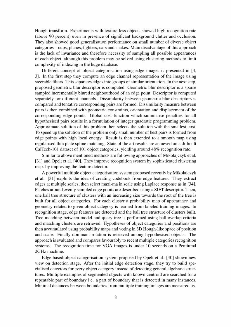
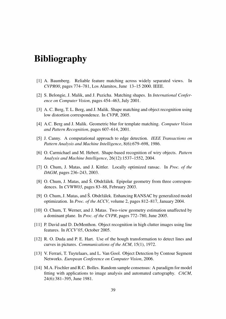
3.5 ExperimentsExperiments were performed on three different scenes see Fig. 3.1 each scene containedsix images with increasing distortion.
3.5.1 Evaluation MethodTo evaluate the performance of detectors we have chosen method based on estimationof surface overlap of regions neighborhoods. This method is in depth described in [33]and frequently used for performance comparison of region based detectors.
Let us assume that for each pair of images I1, I2 of a planar scene a homographyH12 is known. A sets of extremal regions R1 and R2 are detected for each image. Letthe sets X1 and X2 be detected regions that lie in a part of the scene visible in bothimages. Let us denote by ε an overlap error of two regions
ε = 1− intersection(AT EiA ,Ej)
union(AT EiA ,Ej), (3.4)
where Ei and Ej are ellipses defined by covariance matrices of the regions Qi ∈ X1
and Qj ∈ X2 and A is a linearized homography H12 in the centroid of Qi. In ourexperiments corresponding regions are required to have overlap error ε < 0.4. Let C(ε)be the set of corresponding regions based on stable pairing of the regions with smallestoverlap error. For each pair of images we can define ε-repeatability rate as
r(ε) =|C(ε)|
min(|X1|, |X2|). (3.5)
19
The ε-repeatability rate is however is only one view on detector’s performance an-other important measure is the number of repeated regions. Clearly a detector can pro-duce only small number of highly reliable regions and end up with high repeatabilityrate. If these few regions are occluded or not visible in one of the images it will failcompletely. Therefore, together with the repeatability rate we present the number ofcorresponding regions.
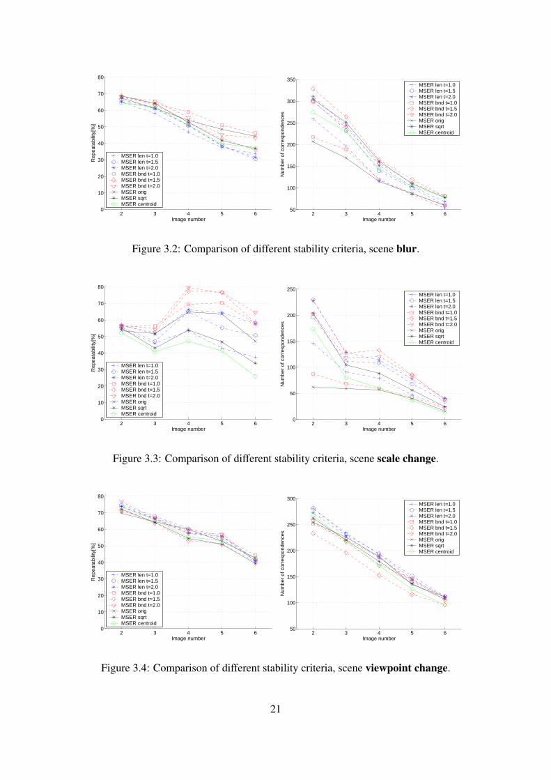
Method identifier Stability thresh. t Criteria of stabilityMSER len t=1.0 1.0 length of boundary Slength
MSER len t=1.5 1.5 length of boundary Slength
MSER len t=2.0 2.0 length of boundary Slength
MSER bnd t=1.0 1.0 number of boundary pixels Sboundary
MSER bnd t=1.5 1.5 number of boundary pixels Sboundary
MSER bnd t=2.0 2.0 number of boundary pixels Sboundary
MSER orig 1.0 percentage of area Sarea
MSER sqrt 1.0 square root of area Ssqrt
MSER centroid 1.0 centroid and compactness stability
Table 3.1: Overview of tested MSER detectors.
3.5.2 Boundary Length EstimationThis experiment compares the repeatability of MSERs with different methods of bound-ary length estimation. First method denoted by Sarea that implements Eqn. 3.1 keepsthe change in area |Qi+∆ −Qi−∆| to be proportional to the area |Qi−∆| at the intensityi−∆. Simple modification Ssqrt estimates the length of boundary as the square root ofthe area Bi =
√|Qi−∆|. The idea mentioned in section 3.4.1 is realised in two different
ways. First method Slength estimates variable Bi as the length of boundary, taking intoaccount all the elementary pixel boundaries e.g. one pixel has border length four, twoneighbouring pixels length of boundary six. Second method Sboundary computes Bi asthe number of pixels on the region’s boundary. Both methods were tested with threedifferent thresholds on q(i). Summary of all tested methods is shown in Tab. 3.1. Inthis experiment three values of ∆ were used on each image pair with similar results.Results for ∆ = 5 are show in Fig. 3.2, Fig. 3.3 and Fig. 3.4.
In terms of number of regions and repeatability rate, estimation of boundary usingnumber of pixels on boundary of the object outperformed method that uses length ofthe boundary. The similar number of correspondences for the corresponding values ofthreshold t indicates the superior performance of this method. The only exception isscene with viewpoint change where all methods achieved similar results.
3.5.3 Sensitivity to BlurSensitivity to blur of the proposed stability criteria was tested on scene blur. It hasshown that in case of blured images, most successful is the method that uses stabil-ity based on number of pixels on the boundary of the extremal region. On the otherside, currently used stability method that uses length of boundary performed well on
20
2 3 4 5 60
10
20
30
40
50
60
70
80
Rep
eata
bilit
y[%
]
Image number
MSER len t=1.0MSER len t=1.5MSER len t=2.0MSER bnd t=1.0MSER bnd t=1.5MSER bnd t=2.0MSER origMSER sqrtMSER centroid
2 3 4 5 650
100
150
200
250
300
350
Num
ber
of c
orre
spon
denc
es
Image number
MSER len t=1.0MSER len t=1.5MSER len t=2.0MSER bnd t=1.0MSER bnd t=1.5MSER bnd t=2.0MSER origMSER sqrtMSER centroid
Figure 3.2: Comparison of different stability criteria, scene blur.
2 3 4 5 60
10
20
30
40
50
60
70
80
Rep
eata
bilit
y[%
]
Image number
MSER len t=1.0MSER len t=1.5MSER len t=2.0MSER bnd t=1.0MSER bnd t=1.5MSER bnd t=2.0MSER origMSER sqrtMSER centroid
2 3 4 5 60
50
100
150
200
250
Num
ber
of c
orre
spon
denc
es
Image number
MSER len t=1.0MSER len t=1.5MSER len t=2.0MSER bnd t=1.0MSER bnd t=1.5MSER bnd t=2.0MSER origMSER sqrtMSER centroid
Figure 3.3: Comparison of different stability criteria, scene scale change.
2 3 4 5 60
10
20
30
40
50
60
70
80
Rep
eata
bilit
y[%
]
Image number
MSER len t=1.0MSER len t=1.5MSER len t=2.0MSER bnd t=1.0MSER bnd t=1.5MSER bnd t=2.0MSER origMSER sqrtMSER centroid
2 3 4 5 650
100
150
200
250
300
Num
ber
of c
orre
spon
denc
es
Image number
MSER len t=1.0MSER len t=1.5MSER len t=2.0MSER bnd t=1.0MSER bnd t=1.5MSER bnd t=2.0MSER origMSER sqrtMSER centroid
Figure 3.4: Comparison of different stability criteria, scene viewpoint change.
21
viewpoint change scene. Method that uses stability criteria based on object’s centroidperforms also well on blured images, but its performance drops down on a scene withsignificant change of scale. Originally proposed method in [28] was outperformed byother methods in most of the tests.
3.6 ConclusionsNew stability criteria in a state of the art MSER detector were proposed and comparedwith the original MSER detector. Experiments on target scenes has shown increase inrepeatability rate of about ten to twenty percent while the number of detected regionswas similar or higher than for currently used MSER detector. This enhancement can beused in future to improve performance in object recognition from video sequences.
22
Chapter 4
Integrating Perceptual Grouping andIndexing
Recognition of texture-less and wiry objects is a tricky problem for appearance basedmethods i.e. the approach of Obdrzalek et al. that uses MSER regions described inchapter 3. Texture-less objects often do not have any significant local features. Wiry andtubular objects can not be easily segmented from the background and thus recognisedby appearance based methods that rely on repeatability of a local patch.
An edge-based representations have proven to be useful in the context of objectrecognition [26, 42, 34, 6, 40]. Edges seem to be in some sense complementary struc-tures to other region and interest point based features. The major problem of exploitingedges in computer vision is in generation of sufficiently distinctive and robust descrip-tion with respect to e.g. scale. Position of each edge point is precisely localised inthe gradient direction. On the other side, localisation in direction perpendicular to thegradient is very loose, it is thus hard to robustly estimate characteristic scale of theedge. Furthermore, endpoints and junctions of edges are not very reliable in real-worldscenes as well. These difficulties are some of the main issues why the edge-based ap-proaches still does not provide sufficient general solution to fast recognition of wiryand texture-less objects. In chapter 2 we discussed couple of recent approaches to edgebased recognition. Solutions based on multiple views of the object or aiming on cat-egorisation of object class from multiple examples shown plausible recognition rateon solid and textured object classes. Our goal is however to build recognition systemthat is able to fast recognise objects from as few as one or two available model views.To achieve this we have chosen to follow the concept of perceptual grouping [26] andfast indexing [42]. In this chapter we present Channel Representation i.e. detection ofedges using multiple images of elongated steerable image filters. Steerable filters canbe seen as grouping on the lowest level. Higher abstraction layer, grouping of simpleedge primitives - lines and curvature extrema is discussed in section 4.1. Preliminaryresults on simple images are shown in section 4.3.
4.1 Perceptual Grouping and Measurement RegionOne of the problems of edge representation is the lack of scale in other words a difficultyto estimate the size of local neighbourhood. The fundamental idea of our approach is si-
23
133
241
242
5
133
241
242
5
133
203
241
242
133
241242
5
133
241242
5
133
203
241242
Figure 4.1: Growth of corresponding measurement regions in two images.
multaneous computation of repeatable structures - perceptual groupings and estimationof measurement region. Measurement region can be defined as the smallest neighbour-hood of the object that needs to be covered by the grouping and is still distinguishablefrom the other groupings.
4.1.1 RepeatabilityRepeatability can be defined as probability, that detected structures will be repeatedlyfound in the images of the same object or scene taken from different viewpoints. Thisprobability can be more-less properly estimated from a large enough database of im-ages. However simple assumptions can be used to find reasonable approximations fora particular structure. E.g. repeatability of a line is probably related to its length andoverall quality of gradients supporting the line, repeatability of an inflection point canbe estimated from the size of related curvatures, etc.
4.1.2 Measurement RegionThe size of a measurement region is clearly property of a given image or a set of images.E.g. in our definition of the measurement region, its size can grow seriously in presence
24
of repeated structures. Ideally, each image in the database should be distinguished fromthe other in the different classes. While all training images are available in the learningphase, it cannot be known which part of the image belongs to the object and if the objectwill be seen in the same position from the same viewpoint. In presence of this uncer-tainty we assume that sufficient size of the measurement region is the one that allowsto uniquely identify part of object (or object as a whole) between the other objects inthe database. Therefore we propose following approach to estimate proper size of themeasurement region dependent on problem, system is dealing with. Both approachescan be solved by simultaneous indexing and enumeration of possible groupings at givenmeasurement region size.
4.1.3 The Algorithm
Overall algorithm of enumerating groupings and estimating measurement region worksas follows:
1. First step is the detection of simple and reliable features - primitives that locallydescribe object’s shape e.g. lines, arcs, extrema of curvature, inflection points etc.Each element is provided with an estimate of repeatability - probability that theelement can be redetected. The estimate is based on measurements made throughthe detection of the primitives (e.g. length for lines, curvature, mutual angle,distance...)
2. In second step, basic relations between detected primitives e.g proximity, connec-tivity or colinearity are established. Basic groupings of primitives are formed anddescribed using affine or similarity invariants. A quality of groupings is calcu-lated from the properties of particular relation. Independence of “repeatabilities”is assumed. E.g. for proximity, repeatability is the product of the repeatabilitiesof the primitives, the probability of having N elements in close neighbourhoodand the probability that the elements in distance D are related.
3. Descriptions of elementary groupings are clustered according to similarity (e.g.Manhattan distance). This can be done using fast hashing table. One part of theclusters with a high number of groupings is considered ambiguous and selectedfor the next step of forming more complex descriptions. While the other part withlower number of groupings is left aside. These groupings are considered distinc-tive within the learned image or image database. The ambiguous groupings aresorted according to estimated the repeatability and the least repeatable groupingsare discarded.
4. A set of possible neighbours using grouping relations is enumerated. A neigh-bouring element with the highest repeatability is chosen and grouping is extended.New estimate of repeatability is calculated. If a maximum size of a grouping isreached, algorithm stops, otherwise step three is taken with the set of more com-plex groupings.
25
Figure 4.2: Image pair used in experiments.
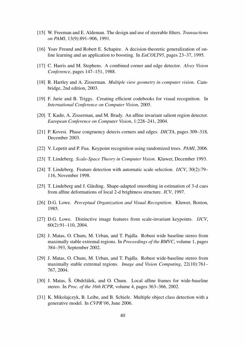
Indexing and Matching
Proposed algorithm produces groupings of different number of elements i.e. three andmore. In indexing step, groupings are clustered by the number of elements into separatehash tables. The hash keys are computed from the affine invariant description of thegrouping. The affine invariant description of the grouping is computed by the followingprocedure. First centered second moments of all point positions are computed andnormalised to unit circle. In the second step the centers of line elements are sortedbased on their distance from the centroid of all points and their normalised positionused as key into hash table. The resulting hash tables for each size of the measurementregion are stored as the learned database.
In recognition phase groupings are formed from a sample image. Each grouping in-dexes into database and a hash bins with similar groupings is found. If there are group-ings belonging to a one class of an object or one sample image, vote for this imagepair is accumulated. Otherwise grouping’s measurement region is extended, groupingis passed to the next level hash table and matched against groupings with bigger mea-surement region. The growth of two matching groupings (with their second momentmatrices visualised as ellipses) used to generate affine invariant description is shown inFig. 4.1.
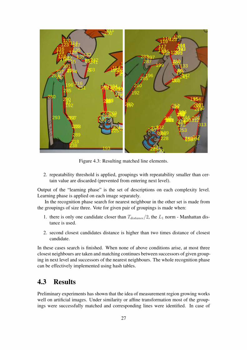
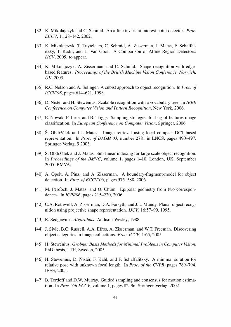
4.2 ExperimentsA partial implementation of the system was developed to prove some concepts of pro-posed algorithm. Currently it contains only line primitives and groupings based onrelation of proximity. Experiment is run on a pair of images. First an edge representa-tion is computed based on [5] edge detector. Then edgel graph is pruned from small andambiguous structures and lines are fitted using least squares fit. Afterwards relation ofproximity is established with fixed distance threshold. Repeatability of line segmentsand proximity relations are estimated using above-mentioned ideas. Learning algorithmis implemented for a single image, with following limitations on size of measurementregion and range expanded groupings:
1. size of measurement region is limited to level 10 (groupings of 10 primitives)
26
215
232
89
88
257
258197
192
199
196204
135
87 244236
130
147
86
282
268
119
242241117118
133
240
125
5203
194
306 63
85
302
303
154161
301
202
116
156
123120
270267
219
290
124
383 26
15
195
285
266
122
287283
269293
280
114
251216
4
172165
273
211200
109
320
47
239225221289
286
218
228
193238
397
215
232
89
88
257
258
197
192
199
196
204
135
87
244236
130
147
86
282
268
119
242241
117118
133
312
240
125
5203
194
306 63
85
302303
154161
301
202
116
156
123120
270267
219
290
124
253
176
158
195
285
323274266
122
287283
293
280
114
172
165
163
273211
200
109
320
317
313
246
47
239225221
188108104228
397
Figure 4.3: Resulting matched line elements.
2. repeatability threshold is applied, groupings with repeatability smaller than cer-tain value are discarded (prevented from entering next level).
Output of the “learning phase” is the set of descriptions on each complexity level.Learning phase is applied on each image separately.
In the recognition phase search for nearest neighbour in the other set is made fromthe groupings of size three. Vote for given pair of groupings is made when:
1. there is only one candidate closer than Tdistance/2, the L1 norm - Manhattan dis-tance is used.
2. second closest candidates distance is higher than two times distance of closestcandidate.
In these cases search is finished. When none of above conditions arise, at most threeclosest neighbours are taken and matching continues between successors of given group-ing in next level and successors of the nearest neighbours. The whole recognition phasecan be effectively implemented using hash tables.
4.3 ResultsPreliminary experiments has shown that the idea of measurement region growing workswell on artificial images. Under similarity or affine transformation most of the group-ings were successfully matched and corresponding lines were identified. In case of
27
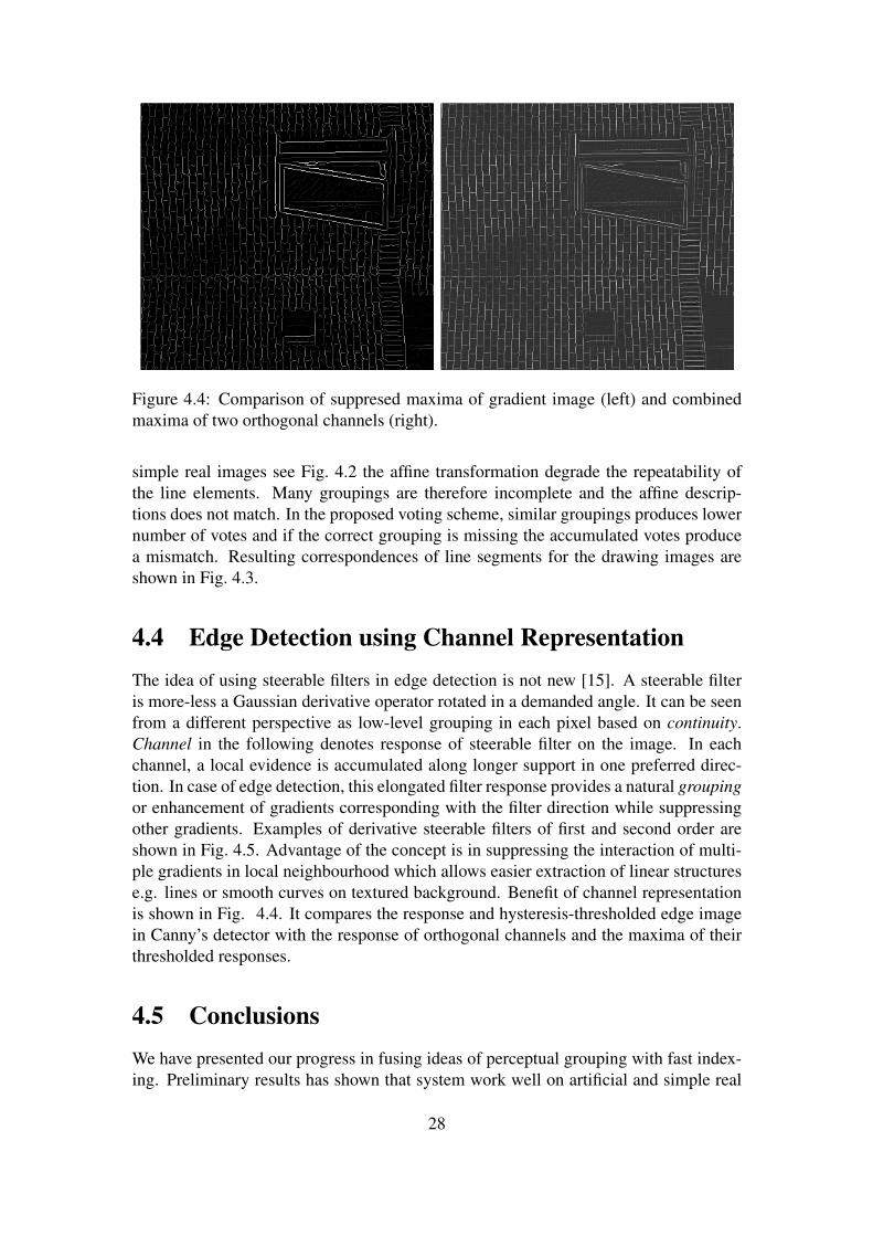
Figure 4.4: Comparison of suppresed maxima of gradient image (left) and combinedmaxima of two orthogonal channels (right).
simple real images see Fig. 4.2 the affine transformation degrade the repeatability ofthe line elements. Many groupings are therefore incomplete and the affine descrip-tions does not match. In the proposed voting scheme, similar groupings produces lowernumber of votes and if the correct grouping is missing the accumulated votes producea mismatch. Resulting correspondences of line segments for the drawing images areshown in Fig. 4.3.
4.4 Edge Detection using Channel RepresentationThe idea of using steerable filters in edge detection is not new [15]. A steerable filteris more-less a Gaussian derivative operator rotated in a demanded angle. It can be seenfrom a different perspective as low-level grouping in each pixel based on continuity.Channel in the following denotes response of steerable filter on the image. In eachchannel, a local evidence is accumulated along longer support in one preferred direc-tion. In case of edge detection, this elongated filter response provides a natural groupingor enhancement of gradients corresponding with the filter direction while suppressingother gradients. Examples of derivative steerable filters of first and second order areshown in Fig. 4.5. Advantage of the concept is in suppressing the interaction of multi-ple gradients in local neighbourhood which allows easier extraction of linear structurese.g. lines or smooth curves on textured background. Benefit of channel representationis shown in Fig. 4.4. It compares the response and hysteresis-thresholded edge imagein Canny’s detector with the response of orthogonal channels and the maxima of theirthresholded responses.
4.5 ConclusionsWe have presented our progress in fusing ideas of perceptual grouping with fast index-ing. Preliminary results has shown that system work well on artificial and simple real
28
Figure 4.5: Steerable filters of first and second order.
images, but fails on more complex real images. The main reason of the failure is unre-liable detection of low level elements - line segments in complex real world scenes. Wehave started to improve detector of line segments using channel representation that canhelp with the detection of segments. However it seems that another concepts of machinelearning and local feature approaches will be needed to achieve reasonable performanceon real scenes.
29
Chapter 5
Epipolar Geometry from TwoCorrespondences
Verification of object pose hypothesis in 3D is an important task in object recognition.Estimation of an epipolar geometry is one way how to verify position of a 3D object inthe scene based on multiple correspondences between the image and the object model.As a rule, local feature based methods establish correspondence of entities which pro-vide geometric constraints stronger than a single point-to-point correspondence. Forinstance, the popular SIFT keypoint operator [27] determines a location, scale and ori-entation; the latter two quantities implicitly define a second point. The LAF-MSER
method of Obdrzalek et al. [30] exploits local affine frames (LAFs), i.e. three orderedpoints detected in an affine-covariant way.
The seven point algorithm embedded in RANSAC is a standard method for epipolargeometry estimation [18]. chum and matas [7, 9] studied whether the required sevenpoint-to-point correspondences obtained from three correspondences of LAFs allowsefficient estimation of epipolar geometry. Since the speed of RANSAC is inversely pro-portional to an exponential function of the sample size, drawing at random three LAF
instead of seven point-to-point correspondences potentially reduces running times byorders of magnitude. The key issue is whether the spatial distribution of the nine points– three triplets of nearby point in a LAF – allows good estimates of epipolar geometry.Experiments in [9] show that standard RANSAC fails in this case. However, a simplemodification called local optimisation of the so-far-the-best solution leads to an algo-rithm that benefits from the small sample size without losing efficiency; speed-ups ofup to 103 are reported.
In this chapter, we take the approach to an extreme and design an algorithm thatcomputes EG from two correspondences of local affine frames using the recently pro-posed 6-point EG estimation algorithm of Stewenius et al. [45, 46]. The new 2LAF-LO-RANSAC algorithm is shown experimentally to have competitive performance, requir-ing a very small number of RANSAC iterations even in situations with a low inlier ratio.The low inlier ratio is common in object recognition when part of the object is occludedand/or object covers only a small part of the image and similar structures may result inmany mismatches.
The rest of the chapter is structured as follows. In Section 5.1 the structure of the2LAF-LO-RANSAC algorithm and its components are described in detail. Experiments
30
CO - Corner (160 inliers in 626 corrs.) BO - Box (335 inliers in 1472 corrs.)
CW - China Wall (106 inliers in 380 corrs.) WA - Wash1(137 inliers in 591 corrs.)
Figure 5.1: Images pairs and characteristics of problems used in experiments.
presented in Section 5.2 validate the design decisions and evaluate performance of thealgorithm. The chapter is concluded in Section 5.3.
5.1 AlgorithmWe first introduce the building blocks of the 2LAF-LO-RANSAC algorithm: the RANSAC
estimator [14], the local optimisation for RANSAC [7], a method detecting degeneratedconfigurations [10] and the six-point solver for EG [45, 46].
RANSAC is a simple but powerful algorithm. Repeatedly, subsets are randomly se-lected from input data T and model parameters θ fitting the sample are computed. Thesize m of the random samples is the smallest sufficient for determining model param-eters. In a second step, the quality of the model parameters is evaluated on the fulldata set. Different cost functions may be used [48], the standard being the size of thesupport, i.e. the number of data points consistent with the model. The process is termi-nated when the likelihood of finding a better model becomes low, i.e. the probability ηof missing a set of inliers I of size I within k samples falls under predefined thresholdη0
η = (1− P (I))k. (5.1)
The probability P (I) that an uncontaminated sample of size m is randomly selectedfrom N = |T | correspondences is
P (I) =
(Im
)(Nm
) =m−1∏j=0
I − j
N − j≈ εm, (5.2)
where ε is the fraction of inliers ε = I/N . Let the support S(θ, T , ∆) : Θ → T be theset of data points consistent with model θ i.e.
S(θ, T , ∆) = {x ∈ T |ρ(θ,x) ≤ ∆},
31
where ρ(θ,x) is a distance measure (e.g. Sampson’s error [18]) and ∆ a user-specifiedthreshold. The average number of samples that has to be drawn to satisfy η ≤ η0 is
kη0(Sk) =
ln(η0)
ln(1− P (Sk)). (5.3)
LO-RANSAC (RANSAC with local optimisation). Note that the expression for probabil-ity η controlling RANSAC termination as defined by Equations (5.1) and (5.2) is validonly under the assumption that a selection of any random sample not contaminated byoutliers leads to the correct solution, i.e. to a solution supported by all inliers. However,as shown in [7], this assumption is often invalid. For standard 7-point and 8-point EG
estimators, all-inlier samples fail at a rate that can be unnoticed and/or ignored2, despitethe fact that the rate is not negligible — Murray and Tordoff [47] observed that abouttwo to three times more samples were needed than predicted by theory. For algorithmsthat estimate EG from LAFs, we observed that the percentage of all-inlier samples lead-ing to a correct EG estimate is negligible, less than 0.1% on the scenes shown in Fig. 5.1!This observation is consistent with [9], which demonstrates that EG cannot be efficientlycomputed form three LAF correspondences by standard RANSAC. However, it is alsoshown in [7] that the so called ”local optimisation” overcomes the problem. We show,if an appropriate local optimisation is adopted, the result also holds for the six pointsolver [46] estimating EG from two LAF correspondences.
The core insight of LO-RANSAC is the following. For the success of a particu-lar estimator within a RANSAC framework, it is not necessary that any all-inlier samplegenerates an EG hypothesis that is close to optimal. It is sufficient if a significant propor-tion of EGs estimated from all-inlier samples has support higher (more correspondencesconsistent with it) than almost all EGs estimated from contaminated samples, i.e. EGswith random support. If this property holds, an EG hypothesis from an all-inlier sampleis very likely to be so-far-the-best, i.e. it is the EG with the largest support observed sofar. It is proved in [7] that as the RANSAC progresses, only very few so-far-the-best EG
hypothesis emerge. It is therefore possible to apply even fairly complex optimisationprocedures on the so-far-the-best model without affecting overall time complexity.
Degeneracy. The presence of degenerate configurations is a surprisingly commonmode of failure of RANSAC. A (dominant) plane is a typical degenerate configurationin EG estimation – EG cannot be recovered from a coplanar, even an all-inlier one. In[10], it was shown that even if a part of a sample (at least five points out of a seven pointsample) lies in a plane, the estimated EG may be incorrect and yet having significantlyhigher than random support. Unsurprisingly, the problem of degenerated configurationsis acute if an EG is estimated from a small number (three or two) of LAFs. The smallerthe sample the higher the probability that the whole sample comes from a single plane.Potential degeneracy is therefore checked for each so-far-the-best sample, as suggestedin [10]. When a planar configuration is detected, the plane-and-parallax [10] algorithmis exploited to estimate the EG.
Six point solvers in 2LAF-LO-RANSAC. Two LAFs [30] provide six point-to-pointcorrespondences. Practical six point solvers have been recently introduced [45, 46].We adopted the algorithm [46], since it has the least restrictive assumptions about the
1Images of Wash were gracefully provided by Tinne Tuytelaars.2At least the problem has not been often reported in the literature.
32
Algorithm 3: The structure of LO-RANSAC with the degenerated configurationtest.
Input: set of data points T , thresholds η0 , ∆Output: model θ∗ with largest support S∗
1. repeat2. Draw a random sample of minimal size m from data points T .3. Model parameters θi computed from the minimal set by estimator E.4. Calculate the support Si of the model θi.5. if new maximum has occurred (|Si| > |Sj| for ∀j < i):6. if a degenerated configuration is detected7. Perform plane-and-parallax search for EG and appropriate lo-
cal optimisation.8. otherwise9. Apply local optimisation.
10. Store the best model θ∗ with support S∗.11. until the probability η of finding model with support larger than S∗ falls
under η0 .
camera. In [46], it is assumed that the intristic camera parameters are known up toa common focal length f . We assume that the (unknown) intristic parameters are: aunit aspect ratio, zero skew, and the principal point in the center of the image. Suchan approximation is reasonable for many currently used sensors. Experimentally, weshow that the algorithm is not affected by slight deviation from the model (i.e. differentfocal length, rectangular pixels see Exp. 5.2). Note, that the EG based on the assump-tions on actually unknown intristic parameters is only used as an approximation of thefundamental matrix F. Such an approximation allows generation of reasonable initialhypotheses while reducing the sample size to two LAF correspondences.
5.1.1 2LAF-LO-RANSAC algorithm
The 2LAF-LO-RANSAC algorithm is an instance of LO-RANSAC with a test for a de-generated configuration. Its structure is summarized in Alg. 3; the parameters are: Tis a set of LAF correspondences, the minimal size m = 2, the estimator E is the sixpoint solver [46]. Handling of degenerated configurations [10] proceeds as follows. Ifa non-random number of correspondences consistent with a homography H is found, aplane-and-parallax method [10] is employed. A LAF correspondence outside the planeis sought by RANSAC sampling tentative correspondences off the plane. If a correspon-dence is found that leads to an EG with support significantly (i.e. non-randomly) largerthan the support of the original H-dominated estimate, the plane and parallax algorithmis successful.
33
5.2 Experimental resultsFour scenes (Fig. 5.1) with different number of correspondences and inlier ratios werechosen to evaluate efficiency and performance of the 2LAF-LO-RANSAC algorithm. Inall experiments, LAFs on maximally stable extremal regions [28] were detected andthree point tentative region correspondences (T ) established as in [30]. The quality oftentative correspondences was artificially degraded by untuning the parameters of thematching process.
Abbrev. Estim. Degen. test Data points7PTS 7pt
√7x LAF centers
3LAF 8pt√
3x LAF
3LAF ND 8pt − 3x LAF
2LAF 6pt√
2x LAF
2LAF ND 6pt − 2x LAF
Table 5.1: LO-RANSAC variants used.
A reference model θr of EG was computed using seven point LO-RANSAC and aset Ir, correspondences consistent with θr was stored (see Fig. 5.1). Compared LO-RANSAC variants are listed in Tab. 5.1.
Experiment 1 (Efficiency of 2LAF-LO-RANSAC). In theory, i.e. according toequation (5.2), drawing minimal samples of size m = 2 should increase the probabilityP (I) and significantly reduce the expected average number of samples k (Eqn. 5.3). Inpractice, a certain fraction of all-inlier samples will lead to random EG due to the influ-ence of noise, poor conditioning and violated assumptions e.g. of equal focal lengths.We define efficiency of a LO-RANSAC variant as the fraction of the all-inlier samples thatleads to a model with support size (approximately) equal to I . To measure and comparethe efficiency, the following synthetic experiment (see Tab. 5.2) was conducted.
One thousand random all-inlier samples are generated from the inliers of the refer-ence epipolar geometry. For each sample, an initial hypothesis θ0 is computed from aminimal set of data points. Subsequent steps of LO-RANSAC (see Alg. 1) variants withlocal optimisation and degeneracy test are executed. Column θB shows the numberof θ0 hypothesis that are consistent with less than an accidental number of correspon-dences. This fraction of all-inlier hypotheses cannot be distinguished from an outliercontaminated hypothesis and hence degrades the efficiency of LO-RANSAC. The num-ber of degenerated and non-degenerated all-inlier samples is shown in columns θD andθN . Finally, the number of “good” hypothesis is shown in column θG. Hypotheses areconsidered “good” if the number of consistent correspondences is at least 90% of the|Ir|, i.e. the number of inliers of reference EG.
We observed (see Tab. 5.2) that the efficiency of the seven point estimator does notdrop under 65% even on the noisiest scene – Wash. 3LAF-LO-RANSAC and 2LAF-LO-RANSAC performs better on the scenes Corner and Box with higher inlier ratio.On the noisy and hard scenes, their efficiency drops down to around 30% for 3LAF-LO-RANSAC algorithm and 25-30% for 2LAF-LO-RANSAC algorithm. Therefore, toachieve a desired probability of success η0 , the number of samples drawn before termi-nation needs to take efficiency in account. Note however that in the performance test
34
0.5 0.7 1.0 1.25 2.0
70 80 90 100 1100
20
40
60
#inls
#ru
ns
70 80 90 100 1100
20
40
60
#inls
#ru
ns
70 80 90 100 1100
20
40
60
#inls
#ru
ns
70 80 90 100 1100
20
40
60
#inls
#ru
ns
70 80 90 100 1100
20
40
60
#inls
#ru
ns
Figure 5.2: Number of inliers in 100 runs of 2LAF algorithm on China Wall scene withdifferent aspect ratios.
(Exp. 3) theoretical number of samples is used to observe differences between algo-rithms.Scn. Alg. |θB| |θD| |θN | |θG|
Table 5.3: Average number of inliers, sam-ples and number of LOs taken in 100 runsof RANSAC algorithms.
Experiment 2 (The robustness of the 6pt solver). Proposed 2LAF-LO-RANSAC
algorithm uses the six point solver [46] to estimate the initial hypothesis that assumescalibrated cameras up to an unknown common focal length. The first three assumptions:the principal point in the middle of the image, zero skew, and unit aspect ratio often holdwith modern cameras, while the assumption of common focal length is often violated.The sensitivity to different focal lengths is tested on the Corner scene with focal lengthratio of about 3. No significant decrease in performance was observed. Robustness to
35
Corner Box China Wall Wash
7PT
S
80 100 120 140 1600
20
40
60
80
100
150 200 250 300 3500
20
40
60
80
100
60 80 1000
20
40
60
80
100
60 80 100 120 1400
20
40
60
80
1003L
AF
80 100 120 140 1600
20
40
60
80
100
150 200 250 300 3500
20
40
60
80
100
60 80 1000
20
40
60
80
100
60 80 100 120 1400
20
40
60
80
100
3LA
FN
D
80 100 120 140 1600
20
40
60
80
100
150 200 250 300 3500
20
40
60
80
100
60 80 1000
20
40
60
80
100
60 80 100 120 1400
20
40
60
80
100
2LA
F
80 100 120 140 1600
20
40
60
80
100
150 200 250 300 3500
20
40
60
80
100
60 80 1000
20
40
60
80
100
60 80 100 120 1400
20
40
60
80
100
2LA
FN
D
80 100 120 140 1600
20
40
60
80
100
150 200 250 300 3500
20
40
60
80
100
60 80 1000
20
40
60
80
100
60 80 100 120 1400
20
40
60
80
100
Figure 5.3: Number of inliers in 100 runs of RANSAC algorithms. Dashed line delimits90% of inliers according to reference model.
aspect ratio was tested on the China Wall scene. One coordinate was artificially scaledwith factor from 0.5 to 2.0. Similar performance (see Fig. 5.2) was observed for allfactors.
Experiment 3 (The speed of RANSAC algorithms). The speed of 2LAF-LO-RANSAC, 3LAF-LO-RANSAC and seven point LO-RANSAC is summarised in Tab. 5.3.As expected, the average number of samples is highest for the seven point algorithm.For 2LAF-LO-RANSAC algorithm it is around one fourth (i.e. proportional to ε) ofthe 3LAF-LO-RANSAC algorithm and about thousand times less compared to the sevenpoint algorithm on hard scenes.
For deeper insight in the performance of algorithms, the histograms Fig. 5.3 of thesupport size of the model found in each run were computed. Results show that thedegeneracy test and the special local optimisation is necessary for 2LAF-LO-RANSAC
algorithm. The 2LAF-LO-RANSAC algorithm without the degeneracy test, i.e. when the
36
so-far-the-best models are processed only with local optimisation, fail to produce a sta-ble solution on difficult problems. On the China Wall and Wash scenes, approximately40% of executions (see Fig. 5.3) produced solutions with less than 90% of the referencemethod’s support.
5.3 ConclusionsThe 2LAF-LO-RANSAC algorithm that estimates epipolar geometry from two LAF cor-respondences was proposed. Two LAF correspondences provide six point-to-point cor-respondences that are used to generate RANSAC hypotheses by the state-of-the-art 6ptsolver [45, 46]. Experimentally, it was shown that the algorithm performs well only ifthe methods [9, 10] for local optimisation and degeneracy detection are used. Comparedto 3LAF-LO-RANSAC algorithm, the 2LAF-LO-RANSAC algorithm requires lower num-ber of samples, local optimisations, and significantly lower number of iterations thanthe seven point LO-RANSAC with degeneracy test. In experiments where the inlier ratioranged from 23% to 28% the number of iterations ranged from 45 to 70 for 2LAF-LO-RANSAC, 151 to 258 for 3LAF-LO-RANSAC, and 26396 to 99840 for LO-RANSAC.
37
Chapter 6
Summary and Future Work
We have presented an experimentally verified an extension of the state of the art Maxi-mally Stable Extremal Regions detector that is successively used in local features basedrecognition system [39]. Improved robustness to image blur affects usability of thedetector in processing video sequences.
In the next part of the work we have described a prototype system that integratesideas of perceptual grouping and indexing using affine invariant descriptors. Experi-ments shown good performance on artificial images and simple scenes. Performancedecreases on real images due to unreliable detection of image features and low robust-ness of implemented perceptual grouping approach. Preliminary integration of edgedetector based on channel representation into the system shown promising potential,but left many unanswered questions.
Last part of our work was focused on improving robustness of verification process.Proposed algorithm of estimating epipolar geometry from two correspondences can beused in the verification phase of recognition system to estimate and verify object’s 3Dpose.
In the future work we would like to focus on further improvements towards real-time recognition of wiry and texture-less objects. Presented channel representationcan speed up low level computations, improve repeatability of basic elements (lines,curves, curvature extrema) detection and thus reduce the number of possible groupingsto a tractable amount. However, to take advance of this pixel-wise continuity groupinga new mechanism of low level evidence propagation have to be developed.
Studied state of the art methods shows that significant robustness can be attained byusing many examples of the recognised object. These extensively generative approachesmodel prior occurrence probabilities of “visual words” using many observed examples.Modelling the probabilities of repeatable groupings by using local, low level evidenceis a one way of improving bad performance on real images. In our future research wewill look for a solution that will use multiple models to improve stability of perceptualgroupings on real images.
38
Bibliography
[1] A. Baumberg. Reliable feature matching across widely separated views. InCVPR00, pages 774–781, Los Alamitos, June 13–15 2000. IEEE.
[2] S. Belongie, J. Malik, and J. Puzicha. Matching shapes. In International Confer-ence on Computer Vision, pages 454–463, July 2001.
[3] A. C. Berg, T. L. Berg, and J. Malik. Shape matching and object recognition usinglow distortion correspondence. In CVPR, 2005.
[4] A.C. Berg and J. Malik. Geometric blur for template matching. Computer Visionand Pattern Recognition, pages 607–614, 2001.
[5] J. Canny. A computational approach to edge detection. IEEE Transactions onPattern Analysis and Machine Intelligence, 8(6):679–698, 1986.
[6] O. Carmichael and M. Hebert. Shape-based recognition of wiry objects. PatternAnalysis and Machine Intelligence, 26(12):1537–1552, 2004.
[7] O. Chum, J. Matas, and J. Kittler. Locally optimized ransac. In Proc. of theDAGM, pages 236–243, 2003.
[8] O. Chum, J. Matas, and S. Obdrzalek. Epipolar geometry from three correspon-dences. In CVWW03, pages 83–88, February 2003.
[9] O. Chum, J. Matas, and S. Obdrzalek. Enhancing RANSAC by generalized modeloptimization. In Proc. of the ACCV, volume 2, pages 812–817, January 2004.
[10] O. Chum, T. Werner, and J. Matas. Two-view geometry estimation unaffected bya dominant plane. In Proc. of the CVPR, pages 772–780, June 2005.
[11] P. David and D. DeMenthon. Object recognition in high clutter images using linefeatures. In ICCV’05, October 2005.
[12] R. O. Duda and P. E. Hart. Use of the hough transformation to detect lines andcurves in pictures. Communications of the ACM, 15(1), 1972.
[13] V. Ferrari, T. Tuytelaars, and L. Van Gool. Object Detection by Contour SegmentNetworks. European Conference on Computer Vision, 2006.
[14] M.A. Fischler and R.C. Bolles. Random sample consensus: A paradigm for modelfitting with applications to image analysis and automated cartography. CACM,24(6):381–395, June 1981.
39
[15] W. Freeman and E. Aldeman. The design and use of steerable filters. Transactionson PAMI, 13(9):891–906, 1991.
[16] Yoav Freund and Robert E. Schapire. A decision-theoretic generalization of on-line learning and an application to boosting. In EuCOLT95, pages 23–37, 1995.
[17] C. Harris and M. Stephens. A combined corner and edge detector. Alvey VisionConference, pages 147–151, 1988.
[18] R. Hartley and A. Zisserman. Multiple view geometry in computer vision. Cam-bridge, 2nd edition, 2003.
[19] F. Jurie and B. Triggs. Creating efficient codebooks for visual recognition. InInternational Conference on Computer Vision, 2005.
[20] T. Kadir, A. Zisserman, and M. Brady. An affine invariant salient region detector.European Conference on Computer Vision, 1:228–241, 2004.
[21] P. Kovesi. Phase congruency detects corners and edges. DICTA, pages 309–318,December 2003.
[22] V. Lepetit and P. Fua. Keypoint recognition using randomized trees. PAMI, 2006.
[23] T. Lindeberg. Scale-Space Theory in Computer Vision. Kluwer, December 1993.
[24] T. Lindeberg. Feature detection with automatic scale selection. IJCV, 30(2):79–116, November 1998.
[25] T. Lindeberg and J. Garding. Shape-adapted smoothing in estimation of 3-d cuesfrom affine deformations of local 2-d brightness structure. ICV, 1997.
[26] D.G. Lowe. Perceptual Organization and Visual Recognition. Kluwer, Boston,1985.
[27] D.G. Lowe. Distinctive image features from scale-invariant keypoints. IJCV,60(2):91–110, 2004.
[28] J. Matas, O. Chum, M. Urban, and T. Pajdla. Robust wide baseline stereo frommaximally stable extremal regions. In Proceedings of the BMVC, volume 1, pages384–393, September 2002.
[29] J. Matas, O. Chum, M. Urban, and T. Pajdla. Robust wide-baseline stereo frommaximally stable extremal regions. Image and Vision Computing, 22(10):761–767, 2004.
[30] J. Matas, S. Obdrzalek, and O. Chum. Local affine frames for wide-baselinestereo. In Proc. of the 16th ICPR, volume 4, pages 363–366, 2002.
[31] K. Mikolajczyk, B. Leibe, and B. Schiele. Multiple object class detection with agenerative model. In CVPR’06, June 2006.
40
[32] K. Mikolajczyk and C. Schmid. An affine invariant interest point detector. Proc.ECCV, 1:128–142, 2002.
[33] K. Mikolajczyk, T. Tuytelaars, C. Schmid, A. Zisserman, J. Matas, F. Schaffal-itzky, T. Kadir, and L. Van Gool. A Comparison of Affine Region Detectors.IJCV, 2005. to appear.
[34] K. Mikolajczyk, A. Zisserman, and C. Schmid. Shape recognition with edge-based features. Proceedings of the British Machine Vision Conference, Norwich,UK, 2003.
[35] R.C. Nelson and A. Selinger. A cubist approach to object recognition. In Proc. ofICCV’98, pages 614–621, 1998.
[36] D. Nister and H. Stewenius. Scalable recognition with a vocabulary tree. In IEEEConference on Computer Vision and Pattern Recognition, New York, 2006.
[37] E. Nowak, F. Jurie, and B. Triggs. Sampling strategies for bag-of-features imageclassification. In European Conference on Computer Vision. Springer, 2006.
[38] S. Obdrzalek and J. Matas. Image retrieval using local compact DCT-basedrepresentation. In Proc. of DAGM’03, number 2781 in LNCS, pages 490–497.Springer-Verlag, 9 2003.
[39] S. Obdrzalek and J. Matas. Sub-linear indexing for large scale object recognition.In Proceedings of the BMVC, volume 1, pages 1–10, London, UK, September2005. BMVA.
[40] A. Opelt, A. Pinz, and A. Zisserman. A boundary-fragment-model for objectdetection. In Proc. of ECCV’06, pages 575–588, 2006.
[41] M. Perd’och, J. Matas, and O. Chum. Epipolar geometry from two correspon-dences. In ICPR06, pages 215–220, 2006.
[42] C.A. Rothwell, A. Zisserman, D.A. Forsyth, and J.L. Mundy. Planar object recog-nition using projective shape representation. IJCV, 16:57–99, 1995.
[43] R. Sedgewick. Algorithms. Addison-Wesley, 1988.
[44] J. Sivic, B.C. Russell, A.A. Efros, A. Zisserman, and W.T. Freeman. Discoveringobject categories in image collections. Proc. ICCV, 1:65, 2005.
[45] H. Stewenius. Grobner Basis Methods for Minimal Problems in Computer Vision.PhD thesis, LTH, Sweden, 2005.
[46] H. Stewenius, D. Nister, F. Kahl, and F. Schaffalitzky. A minimal solution forrelative pose with unknown focal length. In Proc. of the CVPR, pages 789–794.IEEE, 2005.
[47] B. Tordoff and D.W. Murray. Guided sampling and consensus for motion estima-tion. In Proc. 7th ECCV, volume 1, pages 82–96. Springer-Verlag, 2002.
41
[48] P. H. S. Torr and A. Zisserman. MLESAC: A new robust estimator with applica-tion to estimating image geometry. CVIU, 78:138–156, 2000.
[49] T. Tuytelaars. Local, invariant features for registration and recognition. PhDthesis, K.U.Leuven - ESAT, Leuven, December 2000.
[50] T. Tuytelaars and L. Van Gool. Matching widely separated views based on affineinvariant regions. Int. J. Comput. Vision, 59(1):61–85, 2004.
[51] J. Zhang, M. Marszalek, S. Lazebnik, and C. Schmid. Local features and kernelsfor classification of texture and object categories: A comprehensive study. InBeyond Patches workshop, in conjunction with CVPR, 2006.