22
Visualisation of head.txt
| Date post: | 16-Dec-2015 |
| Category: |
Documents |
| Upload: | claire-stewart |
| View: | 217 times |
| Download: | 0 times |

Visualisation of head.txt

Data capture
• Data for the head figure was captured by a laser scanner.
• The object is mounted on a turntable, and illuminated by a laser stripe
• The stripe forms a line image in a camera retina. Because laser projector and camera are not in line, the line image is not straight, but “wiggles” according to object depth.
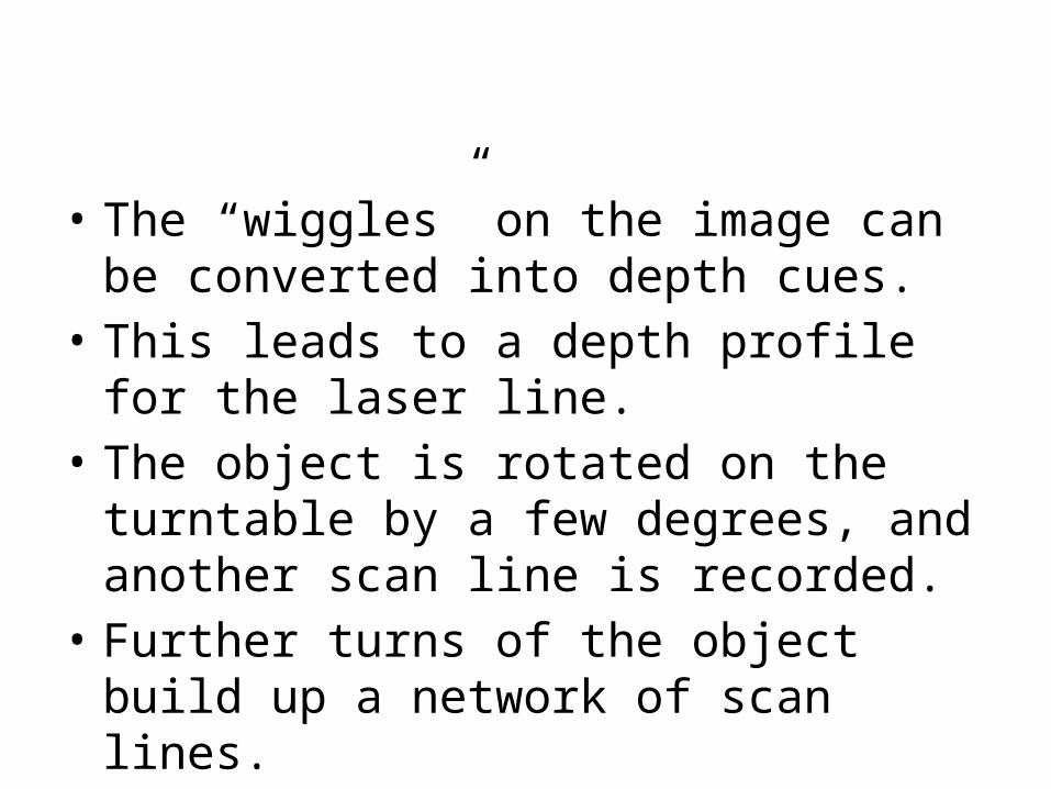
• The “wiggles” on the image can be converted into depth cues.
• This leads to a depth profile for the laser line.• The object is rotated on the turntable by a few
degrees, and another scan line is recorded.• Further turns of the object build up a network
of scan lines.• A view of the scan lines follows.


• The scan lines should be imagined wrapped around a cylinder, whose axis is the axis of rotation of the turntable.
• Equivalently, we can compute the coordinates of the wrapped scan lines as 3D coordinates.
• These are visualised in the next slide.

• Actually, the computed coordinates are for points sampled along the scan lines, at equal vertical distances.
• The capture point coordinates are as shown on the next slide.


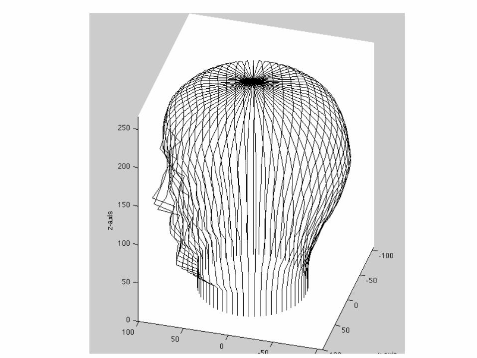
• If we join up not only the points on the same scan line, but also points at the same height across successive scan lines, we get a meshed view of the object.

Az -164El 34

• Except at the “poles”, we get a mesh of 4-sided elementary patches.
• Unfortunately, these patches are not (in general) planes.
• For the purpose of illumination and/or hidden surface removal, planar facets are preferable.
• We can insert a diagonal into each quadrilateral patch, resulting in triangulation.

• Data for the triangulated object (head) was made available in the assignment.
• It consists of a file of vertex coordinates, and a file of vertex connectivities.
• We can now visualise this data. But computing surface normals, we can show just forward facing (and nearest) facets.
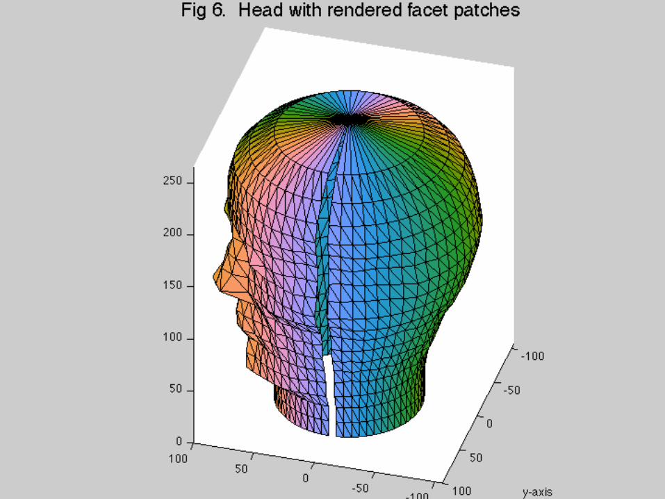


• Note the gap in the object.• This arises because the last (vertical) scan line
falls just short of the first.• We can generate the extra triangles from the
first and last scan lines.• This allows a “joined up” view.

MATLAB program Stage 1
• The visualisations were made in MATLAB.• The program was made to give some feedback• Start and end of facet-vertex list is displayed:

MATLAB program Stage 2
• Start and end of vertex list (coordinate data) is displayed:

MATLAB program Stages 3 and 4
• Do the drawing:

• Here is a view for a different altitude and azimuth.
• Note that one can simulate the views that would be seen by the left and right eyes of an observer, (for a specified position relative to the object).
• This allows the production of stereo (3D) views.


END


