Visualization of Stress Wave Propagation via Air-Coupled ... · Visualization of Stress Wave...

Visualization of Stress Wave Propagation via

Air-Coupled Acoustic Emission Sensors

Joshua C. Rivey, Gil-Yong Lee, Jinkyu Yang

University of Washington, Seattle, Washington, 98195, USA

Youngkey Kim

SM Instruments, Daejon, Republic of Korea

Sungchan Kim

Korea Aerospace Research Institute, Daejon, Republic of Korea

February 2016

Abstract.

We experimentally demonstrate the feasibility of visualizing stress waves propa-

gating in plates using air-coupled acoustic emission sensors. Specifically, we employ a

device that embeds arrays of microphones around an optical lens in a helical pattern.

By implementing a beamforming technique, this remote sensing system allows us to

record wave propagation events in situ via a single-shot and full-field measurement.

This is a significant improvement over the conventional wave propagation tracking ap-

proaches based on laser doppler vibrometry or digital image correlation techniques. In

this paper, we focus on demonstrating the feasibility and efficacy of this air-coupled

acoustic emission technique using large metallic plates exposed to external impacts.

The visualization results of stress wave propagation will be shown under various im-

pact scenarios. Such wave visualization capability is of tremendous importance from a

structural health monitoring and nondestructive evaluation (SHM/NDE) standpoint.

The proposed technique can be used to characterize and localize damage by detecting

the attenuation, reflection, and scattering of stress waves that occurs at damage lo-

cations. This can ultimately lead to the development of new SHM/NDE methods for

identifying hidden cracks or delaminations in metallic or composite plate structures

simultaneously negating the need for mounted contact sensors.

Keywords: sound camera, beamforming, acoustic emission, impact identification

1. Introduction

In aerospace, civil, and mechanical engineering applications, it is imperative to ensure

structural integrity through the detection and characterization of damage and defects.

The presence of defects, such as cracks, dents, corrosion, delaminations, or numerous

other forms of damage, can significantly reduce the inherit properties and performance

arX

iv:1

603.

0629

8v1

[nl

in.P

S] 2

1 M

ar 2

016

Visualization of Stress Waves via Air-Coupled Acoustic Emission Sensors 2

of a structure, thereby increasing the chance of premature failure. Therefore, structural

health monitoring (SHM) and nondestructive evaluation (NDE) have been subjects

of intense studies in recent decades. In particular, increases in the use of advanced

materials, sensors/actuators, and manufacturing processes has spurred the development

of numerous SHM/NDE techniques. These methods include – but are not limited to –

thermography, shearography, X-radiography, eddy current, ultrasonic C-scan, scanning

laser Doppler vibrometry, and guided wave-based ultrasound techniques [1, 2, 3, 4, 5].

They are based on thermal, electromagnetic, acoustic/mechanical, and other multi-

physical feedback, and each technique offers unique advantages and shortcomings.

Using acoustic emissions for purposes of detecting and localizing damage has been

one of the widely adopted methods in the SHM/NDE community [6, 7, 8]. Acoustic

emissions are manifest when a material is subject to extreme stress conditions due

to external loads, such that a local point source within the material suddenly releases

irreversible energy in the form of stress waves. The released stress waves are transmitted

to the surface of the material and then propagate outwards from the epicenter of the

release source. Previous studies on acoustic emission have focused mostly on the onset

of such acoustic emissions to locate their release sources [9, 10, 11, 12]. However, more

useful can be that acoustic emissions are also attenuated, scattered, or reflected by

discontinuities present in the material [8]. We identify that it is this particular property

of acoustic emissions that can be exploited in order to detect and localize pre-existing

damage in an inspection medium.

In this study, we experimentally demonstrate the feasibility of visualizing stress

waves in an aluminum plate using acoustic emissions. The focus is whether acoustic

emission techniques can capture the scattering of stress waves due to the presence of

damage resulting from an applied impact on the plate. For visualizing such transient

events, we employ a device – referred to as an acoustic or sound camera – that embeds an

optical lens at the center and arrays of microphones around the optical lens in a helical

pattern [21]. Note that arrays of microphones have been used in previous studies to

identify the locations of vibration sources [13], but it has not been thoroughly explored

yet to visualize stress waves in structures via air-coupled microphone sensors to the best

of the authors’ knowledge. This is because of a short characteristic time – in the order

of micro-seconds – of stress waves propagating in solids and also due to the difficulty in

capturing and visualizing the wavefronts of these stress waves.

To address the challenges associated with stress wave visualization, we implement

time-domain delay-sum beamforming techniques [14] based on acoustic emission

information collected from the arrays of microphones. To enhance the accuracy of the

diagnostic scheme, we conduct parametric studies on various post-processing conditions,

including the temporal resolution of the sensor data and the spatial resolution of the

inspection plate. Finally, the developed technique is evaluated for SHM/NDE purposes

with capabilities assessed for detecting the defect location simulated with a mass placed

in the path of the wave propagation on the inspection plate.

The acoustic emission beamforming technique coupled with the sound camera


device has unique advantages compared to the conventional techniques such as ultrasonic

or laser based testing methods [6]. Many of the conventional testing methods are

founded on the principle of imparting external stimuli or excitations on the inspection

material and measuring differences in the received signal in order to detect whether

damage is present and where it is located. While such methods generally provide highly

accurate results, they often involve slow and expensive processes to operate equipment.

Conversely, acoustic emission beamforming methods can be conducted in situ and

in real time, without necessitating permanently mounted contact sensors or baseline

data. Recently, laser Doppler vibrometry has gained significant attention as a means

to visualize stress waves in solids and structures with an unprecedented resolution [15,

16, 17]. However, this method requires synchronization and reconstruction of data

measured from every single discretized spatial point of an inspection medium. This

is not practical given the difficulties in exciting structures in a repeated, identical

fashion. Digital image correlation techniques can also visualize extremely dynamic

motions, but they require speckle patterns on specimens and their field of view can

be often narrow for recording high speed events [18]. In contrast, the proposed acoustic

emission beamforming technique is capable of conducting non-contact – yet full-field

– visualization of inspection medium in a single shot measurement. Consequently, we

envision that this method can open new avenues to diagnosing the existence of damage

in structures in a time- and cost-efficient manner by conducting simple tests.

The contents of this manuscript will address the following topics. Section 2 contains

an introduction to the time-domain delay-sum beamforming theory and a discussion of

how this concept is incorporated into the study contained herein. Section 3 describes

the experimental setup used for monitoring inspection plates and tracking stress waves

using the sound camera. Section 4 provides an analysis of parametric studies performed

on pristine plates that were used to determine temporospatial resolutions necessary for

capabilities-centric analyses. Finally, Section 5 concludes the study with an analysis of

the acoustic emission beamforming method for identifying varying impact locations and

detecting simulated damage on the inspection plate.

2. Theoretical background

Traditional methods of source localization via air-coupled acoustic emission rely on the

assumption that the recording device is pointed at or aimed in the general vicinity of the

emission origin. Acoustic beamforming is an attractive alternative for use in acoustic

feedback NDE as it provides the opportunity to detect the direction of unknown acoustic

emissions associated with failure events across a large spatial domain [19]. While

acoustic beamforming is a relatively new concept for applications related to damage

localization, beamforming using microphone arrays is a standard practice for spatial

isolation of sound sources. The beamforming method – also known as microphone

antenna, phased array of microphones, acoustic telescope, or acoustic camera – is used

extensively for localizing sounds on moving objects and to filter out background noise


in acoustically active environments with stationary sound sources [20].

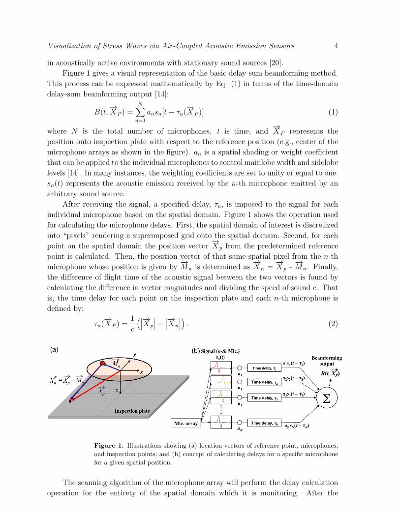
Figure 1 gives a visual representation of the basic delay-sum beamforming method.

This process can be expressed mathematically by Eq. (1) in terms of the time-domain

delay-sum beamforming output [14]:

B(t,−→XP ) =

N∑n=1

ansn[t− τn(−→XP )] (1)

where N is the total number of microphones, t is time, and−→XP represents the

position onto inspection plate with respect to the reference position (e.g., center of the

microphone arrays as shown in the figure). an is a spatial shading or weight coefficient

that can be applied to the individual microphones to control mainlobe width and sidelobe

levels [14]. In many instances, the weighting coefficients are set to unity or equal to one.

sn(t) represents the acoustic emission received by the n-th microphone emitted by an

arbitrary sound source.

After receiving the signal, a specified delay, τn, is imposed to the signal for each

individual microphone based on the spatial domain. Figure 1 shows the operation used

for calculating the microphone delays. First, the spatial domain of interest is discretized

into “pixels” rendering a superimposed grid onto the spatial domain. Second, for each

point on the spatial domain the position vector−→X p from the predetermined reference

point is calculated. Then, the position vector of that same spatial pixel from the n-th

microphone whose position is given by−→Mn is determined as

−→X n =

−→X p -

−→Mn. Finally,

the difference of flight time of the acoustic signal between the two vectors is found by

calculating the difference in vector magnitudes and dividing the speed of sound c. That

is, the time delay for each point on the inspection plate and each n-th microphone is

defined by:

τn(−→XP ) =

1

c

(∣∣∣−→X p

∣∣∣− ∣∣∣−→X n

∣∣∣) . (2)

Figure 1. Illustrations showing (a) location vectors of reference point, microphones,

and inspection points; and (b) concept of calculating delays for a specific microphone

for a given spatial position.

The scanning algorithm of the microphone array will perform the delay calculation

operation for the entirety of the spatial domain which it is monitoring. After the


time delays for all microphones are imposed on the signal for a given spatial pixel,

the transformed signal from each microphone is summed as shown in Figure 1b. The

location of the sound source is determined by the delays for a specific spatial location

which produced the maximum beam output, B(t). It is important to note that the

microphone delays are time independent and therefore will remain constant for a given

microphone to a given spatial pixel throughout the monitoring period assuming the

geometry of the test setup remains constant. While Figure 1 and Equation 1 illustrate

the basic delay-sum beamformer in the time-domain, there exist many variations and

modifications to this algorithm, see reference [14].

3. Experimental setup

For the study presented herein, we used a commercial acoustic emission sensing device

equipped with microphone arrays and a motion camera (SeeSV-S205 Sound Camera,

SM Instruments) [21]. Specifically, the sensing device consisted of a high resolution

optical camera with a sampling rate of 25 frames per second (FPS) located in the center

of the device. The optical camera is surrounded by 30 high sensitivity digital micro-

electric mechanical system (MEMS) microphones with a sampling frequency of 25.6 kHz

arranged in five helical patterns of six microphones each as shown in Figure 2a. The

figure inset shows a digital image of embedded microphones along with the optical lens.

Figure 2b shows the experimental setup used in this study to induce and track the

transient waves in the aluminum plate. The images show the 1.2 m × 1.2 m × 1.02

mm 6061-T6 aluminum plate mounted to an optical table using a rail system to create

a fixed boundary condition around the plate. The plate was secured between the angle

bars and the square tube with fasteners placed every six inches that went through all

pieces to effectively fix the boundary of the plate and suspend it above the optical table.

Figure 2. (a) Arrangement of 30 MEMS microphones and an optical camera. Inset

shows a digital image of the sound camera. (b) Proposed experimental setup for

inducing and tracking transient waves in an aluminum plate using the sound camera.


Once the plate was installed, the acoustic camera was mounted above the

center of the plate at a height of 0.52 m as shown in Figure 2b. Impacts

were introduced into the plate via manually tapping the plate using the tip of a

hexagonal wrench while simultaneously capturing the acoustic signal recorded by the 30

microphones. Afterwards, post-processing was performed to calculate the time delays

and beamforming output based on Equations (1) and (2) in order to produce the acoustic

images.

4. Parametric studies on pristine plates

In this study different parameters were systematically varied to investigate and assess the

wave propagation tracking capabilities of the sound camera in addition to determining

post-processing parameters used in subsequent analyses. These parameters included the

temporal and spatial resolutions in post-processing. This section discusses the results

from these parametric studies given pristine plates. For all images shown of the wave

propagation tracking, the area presented in the image represents that of the entire

inspection plate.

4.1. Effects of temporal resolution

The temporal resolution was investigated with the goal of achieving a smooth

propagation of the transient wave front. In this study, the sound camera MEMS

microphones imposed a hardware limitation on the sampling frequency restricting it

to 25.6 kHz. This meant the time between individual samples was slightly greater than

39 µs. During investigation of wave propagation velocities, the speed of major flexural

waves propagating in the 1.02 mm thick plate was approximately 1,700 m/s (to be

further discussed below). At this wave speed and the given sampling frequency, the

wave front propagated approximately 66.4 mm between each sample or 5.4% of the

total plate width, resulting in a very coarse propagation tracking ability.


Figure 3. Effects of changing temporal resolution using interpolation of results in

frequency domain.(a) Original temporal data and the post-processed surface maps

showing stress wave propagation at t = 0, 0.20, and 0.31 ms. (b) Interpolated temporal

data and the post-processed surface maps showing stress wave propagation at t =

0, 0.20, and 0.31 ms. For all surface maps, the spatial resolution was fixed at 30

mm between adjacent pixels. The colorbar at the bottom shows the intensity of the

beamforming output in Pa.

To reduce the effective propagation distance between sequential samples and to

improve the resolution of the wave propagation tracking, an interpolation of the raw

acoustic signal was performed. Figure 3a shows a window of the raw signal with no

interpolation applied (left panel), in which we observe the drastic amplitude changes of

pressure measured from a microphone between subsequent samples. The beamforming

results of the stress wave propagation for the raw signal without interpolation are shown

in the three images to the right of the signal. The inset image at t = 0 ms in Figure 3a

represents the top left impact induced in the inspection plate.

Figure 3b shows the same raw signal as the one above it, but with a frequency-

domain fast fourier transformation interpolation applied to reconstruct the signal. An

upsample factor of 10 was chosen for the interpolation in order to decrease the time

between samples to 3.9 µs. This meant that the propagation distance between samples

was reduced to 6.6 mm and only 0.5% of the total plate width. The drastic effects of

the interpolation are seen in the series of images to the right of the second signal.

Comparing the two sets of images presented in Figure 3, we find that both

approaches successfully identify the impact location with a reasonably high accuracy

(to be further discussed in the later section). However, the results from the raw signal

do not show clear boundaries of wave front while the second set of images associated with

the interpolated data show the increased definition of the wave front. Additionally, a

significant amount of acoustic background noise was removed in the case of interpolation,


which resulted in a refined beamforming image. Looking at t = 0.20 ms in Figure 3,

it is clear that the wave front amplitude is reduced in the reconstructed signal image.

The decreased amplitude is due to the more accurate representation of the wave front

shape resulting from the interpolation of the acoustic signal. This reduces exaggerated

pressure amplitude changes observed from the original acoustic signal.

While the resolution of the wave propagation was achieved by increasing the

upsample factor, a computational penalty was incurred. Based on parametric studies

on different upsample factors, the upsample-computational time relationship was

approximately linear with an increase in computational time. Specifically, for the

upsample factor of n, the beamforming computational time is increased (0.1044 ±0.014) × n times compared to the original raw signal. The reduced computational

efficiency was deemed an acceptable cost for the increased resolution gained using

the reconstructed signal and necessary for identifying and localizing masses. For all

subsequent simulations, we used an upsample factor of 10.

4.2. Effects of spatial resolution

Now we investigate the effect of spatial resolution in an attempt to further refine

the wave front throughout the propagation time. Figure 4 shows the results of the

spatial resolution study. Here the spatial resolution was systematically halved for each

simulation throughout the parametric study. Figure 4a and subsequent beamforming

images show the results for a spatial resolution (∆X) of 80 mm between pixels. While

the impact point in the surface map is well localized (compare with the actual impact

location as shown in the inset image), the wave front becomes blurry as it begins to

propagate into the far-field as seen at times t = 0.21 ms and t = 0.32 ms.

Figures 4b-c and associated images show spatial resolutions of 40 mm and 20 mm

between pixels, respectively. Both sets of images show an accurate impact localization

and increased definition of the wave front as the spatial resolution increases. Figure 4d

and corresponding wave propagation images represent the case of ∆X = 10 mm between

pixels. Compared to all previous results, these images show a very definitive wave front

at t = 0.21 ms. The image at t = 0.32 ms for a spatial resolution of 10 mm solidifies

that increased spatial resolution can maintain the wave front definition into the far-field

of the plate while post-impact saturation behind the wave front clearly emanates from

the impact location.


Figure 4. Effects of changing spatial resolution by decreasing step size between

“pixels” on virtual inspection plane. Left column shows spatial resolution, while the

next three right columns show surface maps of wave propagation for t = 0, 0.21, and

0.31 ms under the spatial resolution of (a) ∆X = 80 mm; (b) 40 mm; (c) 20 mm; and

(d) 10 mm.

While a 10 mm displacement between adjacent pixels may be excessive by creating

ripples, it increases the chance of detecting an artificially created damage (to be

discussed in Section 5) and accurately determining its location. However for each

halving of the spatial resolution, the computational time is increased by a factor of

approximately 4.25, thereby resulting in an approximately power-law relationship equal

to (2.08 ± 0.042) increase in computational time as the spatial resolution is increased

(that is ∆X decreases). The power-law relationship is due to the spatial resolution

affecting both dimensions of the inspection plate meaning that the increase in spatial

resolution is squared with each iteration. While this leads to a significant increase in

computational time, the increase was again considered as an acceptable trade-off for

the gained wave propagation resolution. This would prove necessary for detecting and


localizing artificially created damage on the plate in subsequent analyses. Following the

temporal and spatial resolution studies, a temporal upsample factor of 10 and a spatial

resolution of 10 mm were selected for use in all following analyses.

5. Feasibility studies on the applications to NDE/SHM

In this section, we assess the feasibility of using the beamforming-based sound camera

technique for (i) identifying impact location for real-time SHM applications and (ii)

detecting artificial damage location for potential NDE applications.

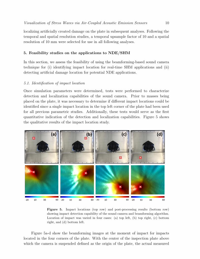
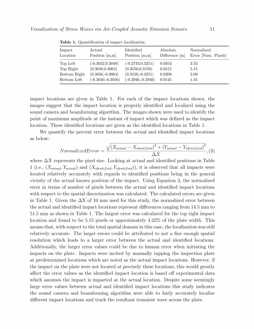
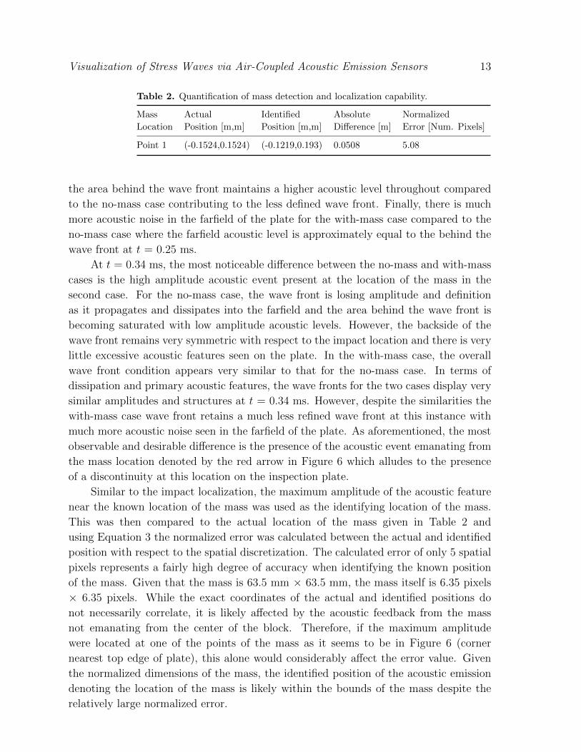
5.1. Identification of impact location

Once simulation parameters were determined, tests were performed to characterize

detection and localization capabilities of the sound camera. Prior to masses being

placed on the plate, it was necessary to determine if different impact locations could be

identified since a single impact location in the top left corner of the plate had been used

for all previous parametric studies. Additionally, these tests would serve as the first

quantitative indication of the detection and localization capabilities. Figure 5 shows

the qualitative results of the impact location study.

Figure 5. Impact locations (top row) and post-processing results (bottom row)

showing impact detection capability of the sound camera and beamforming algorithm.

Location of impact was varied in four cases: (a) top left, (b) top right, (c) bottom

right, and (d) bottom left.

Figure 5a-d show the beamforming images at the moment of impact for impacts

located in the four corners of the plate. With the center of the inspection plate above

which the camera is suspended defined as the origin of the plate, the actual measured


Table 1. Quantification of impact localization.

Impact

Location

Actual

Position [m,m]

Identified

Position [m,m]

Absolute

Difference [m]

Normalized

Error [Num. Pixels]

Top Left (-0.3032,0.3048) (-0.2743,0.3251) 0.0353 3.53

Top Right (0.3048,0.3064) (0.3556,0.3150) 0.0515 5.15

Bottom Right (0.3056,-0.3064) (0.3150,-0.3251) 0.0209 2.09

Bottom Left (-0.3040,-0.3056) (-0.2946,-0.2946) 0.0145 1.45

impact locations are given in Table 1. For each of the impact locations shown, the

images suggest that the impact location is properly identified and localized using the

sound camera and beamforming algorithm. The images shown were used to identify the

point of maximum amplitude at the instant of impact which was defined as the impact

location. These identified locations are given as the identified locations in Table 1.

We quantify the percent error between the actual and identified impact locations

as below:

NormalizedError =

√(Xactual −Xidentified)

2 + (Yactual − Yidentified)2

∆X, (3)

where ∆X represents the pixel size. Looking at actual and identified positions in Table

1 (i.e., (Xactual, Yactual) and (Xidentified, Yidentified)), it is observed that all impacts were

located relatively accurately with regards to identified positions being in the general

vicinity of the actual known position of the impact. Using Equation 3, the normalized

error in terms of number of pixels between the actual and identified impact locations

with respect to the spatial discretization was calculated. The calculated errors are given

in Table 1. Given the ∆X of 10 mm used for this study, the normalized error between

the actual and identified impact locations represent differences ranging from 14.5 mm to

51.5 mm as shown in Table 1. The largest error was calculated for the top right impact

location and found to be 5.15 pixels or approximately 4.22% of the plate width. This

means that, with respect to the total spatial domain in this case, the localization was still

relatively accurate. The larger errors could be attributed to not a fine enough spatial

resolution which leads to a larger error between the actual and identified locations.

Additionally, the larger error values could be due to human error when initiating the

impacts on the plate. Impacts were incited by manually tapping the inspection plate

at predetermined locations which are noted as the actual impact locations. However, if

the impact on the plate were not located at precisely these locations, this would greatly

affect the error values as the identified impact location is based off experimental data

which assumes the impact is imparted at the actual location. Despite some seemingly

large error values between actual and identified impact locations this study indicates

the sound camera and beamforming algorithm were able to fairly accurately localize

different impact locations and track the resultant transient wave across the plate.


5.2. Identification of pre-existing artificial damage

Once it was established that the sound camera could detect and sufficiently track the

transient wave, the impact location was fixed and masses were added to the plate to

determine the capability of the sound camera and beamforming algorithm to detect the

discontinuities which represented psuedo-damage cases. The impact location used is a

top left impact as shown in Figure 6a-b. The mass used for this study was a 0.615 kg,

0.0635 m × 0.0635 m × 0.0196 m stainless steel block. The mass was affixed to the

inspection plate using silicon sealant tape that was applied to the entire contact surface

of the mass. The use of masses to simulate damage has been used on many occasions

to assess the capabilities of different SHM/NDE techniques [22, 23]. Figure 6b shows

the mass was place halfway between the impact location and the center of the plate

meaning the mass was approximately 0.215 m from the impact location. Figure 6 shows

the wave propagation results for the inspection plate without and with mass present.

Figure 6. Beamforming results for plate without and with mass. Results suggest that

sound camera using acoustic beamforming can be used for detection of discontinuities.

Figure 6 uses a red cross and a red square to mark the approximate location of

the impact and mass, respectively, on the plate. At t = 0 ms, the instant of impact

is shown for both the without- and with-mass cases. In these images look very similar

between the two cases and there is no indication of a mass being present on the plate.

The images at t = 0.25 ms show the wave front just after it has propagated past the

location of the mass. The first difference is seen in the wave front definition. While the

no-mass case maintains a smooth and symmetric wave front, the mass case displays a

more turbulent wave front with a flatten of the wave front on the far side of the mass

relative to the impact point. Additionally, the widespread saturation behind the wave

front seen in the no-mass case is not seen in the with-mass case. In the with-mass case,


Table 2. Quantification of mass detection and localization capability.

Mass

Location

Actual

Position [m,m]

Identified

Position [m,m]

Absolute

Difference [m]

Normalized

Error [Num. Pixels]

Point 1 (-0.1524,0.1524) (-0.1219,0.193) 0.0508 5.08

the area behind the wave front maintains a higher acoustic level throughout compared

to the no-mass case contributing to the less defined wave front. Finally, there is much

more acoustic noise in the farfield of the plate for the with-mass case compared to the

no-mass case where the farfield acoustic level is approximately equal to the behind the

wave front at t = 0.25 ms.

At t = 0.34 ms, the most noticeable difference between the no-mass and with-mass

cases is the high amplitude acoustic event present at the location of the mass in the

second case. For the no-mass case, the wave front is losing amplitude and definition

as it propagates and dissipates into the farfield and the area behind the wave front is

becoming saturated with low amplitude acoustic levels. However, the backside of the

wave front remains very symmetric with respect to the impact location and there is very

little excessive acoustic features seen on the plate. In the with-mass case, the overall

wave front condition appears very similar to that for the no-mass case. In terms of

dissipation and primary acoustic features, the wave fronts for the two cases display very

similar amplitudes and structures at t = 0.34 ms. However, despite the similarities the

with-mass case wave front retains a much less refined wave front at this instance with

much more acoustic noise seen in the farfield of the plate. As aforementioned, the most

observable and desirable difference is the presence of the acoustic event emanating from

the mass location denoted by the red arrow in Figure 6 which alludes to the presence

of a discontinuity at this location on the inspection plate.

Similar to the impact localization, the maximum amplitude of the acoustic feature

near the known location of the mass was used as the identifying location of the mass.

This was then compared to the actual location of the mass given in Table 2 and

using Equation 3 the normalized error was calculated between the actual and identified

position with respect to the spatial discretization. The calculated error of only 5 spatial

pixels represents a fairly high degree of accuracy when identifying the known position

of the mass. Given that the mass is 63.5 mm × 63.5 mm, the mass itself is 6.35 pixels

× 6.35 pixels. While the exact coordinates of the actual and identified positions do

not necessarily correlate, it is likely affected by the acoustic feedback from the mass

not emanating from the center of the block. Therefore, if the maximum amplitude

were located at one of the points of the mass as it seems to be in Figure 6 (corner

nearest top edge of plate), this alone would considerably affect the error value. Given

the normalized dimensions of the mass, the identified position of the acoustic emission

denoting the location of the mass is likely within the bounds of the mass despite the

relatively large normalized error.


6. Conclusions

This study demonstrated the visualization of stress wave propagation across an

aluminum plate using an air-couple microphone array. The scope of the beamforming

method for visualizing stress waves was investigated through various parametric studies

that resulted in the establishment of post-processing parameters of upsample factor

and spatial resolution for further testing. Subsequent testing revealed the ability of

the sound camera to accurately identify various impact locations on the inspection

plate. Finally, the beamforming method was used to detect and localize a mass on

the inspection plate used to simulate the presence of damage. The sound camera and

derived beamforming method were able to relatively accurately locate the position of the

mass through the detection of acoustic emission structures indicating the existence of a

discontinuity on the inspection plate. This study showed the potential for an acoustic

emission beamforming based method to be used for damage detection in SHM/NDE

applications. While this study focused on the feasibility of the proposed technique,

further studies need to be conducted to find more sophisticated beamforming techniques

and to optimize their post-processing parameters. Corresponding experiments will be

also conducted in comparison to other experimental techniques, such as laser Doppler

vibrometry and digital image correlation techniques. Lastly, the authors also plan to

perform numerical studies of air-coupled acoustic emission events using finite element

analysis.

Acknowledgments

This research was supported by INNOPOLIS Foundation grant funded by the Korean

government (Ministry of Science, ICT & Future Planning, Grant number: 14DDI084)

through SM Instruments Inc. We also acknowledge the research grant from the Joint

Center for Aerospace Technology Innovation (JCATI) from Washington State in the

USA. We thank researchers at SM Instruments, including InKwon Kim and JunGoo

Kang, for their technical assistance.

References

[1] Giurgiutiu V 2015 Structural Health Monitoring of Aerospace Composites (Academic Press).

[2] Johnson S B 2011 System Health Management: With Aerospace Applications (John Wiley & Sons,

Ltd)

[3] Wang M L, Lynch J P, Sohn H 2014 Sensor Technologies for Civil Infrastructures: Applications in

Structural Health Monitoring (Woodhead Publishing)

[4] The American Society for Nondestructive Testing, Introduction to Nondestructive Testing, Web,

2015.

[5] B. Boro Djordjevic, Nondestructive Test Technology for the Composites, The 10th International

Conference of the Slovenian Society for Non-Destructive Testing, pages 259-265, Materials and

Sensors Technologies Inc., 2015.

[6] NDT Resource Center, Introduction to Acoustic Emission Testing, National Science Foundation -

Advanced Technological Education.


[7] P Rizzo, F Lanza di Scalea, Acoustic emission monitoring of carbon-fiber-reinforced-polymer bridge

stay cables in large-scale testing, Experimental Mechanics, 41:3, 282, 2001.

[8] Charles Hellier, Handbook of Nondestructive Evaluation: Chapter 10 - Acoustic Emission Testing,

McGraw Hill, 2nd Edition, 2012.

[9] Gregory C. McLaskey, Steven D. Glaser, Christian U. Grosse, Acoustic Emission Beamforming for

Enhanced Damage Detection, Sensors and Smart Structures Technologies for Civil, Mechanical,

and Aerospace Systems, Proc. of SPIE Vol. 6932(39):1-9, 2008.

[10] Christian U. Grosse, Acoustic Emission Localization Methods for Large Structures Based on

Beamforming and Array Techniques, Non-Destructive Testing in Civil Engineering, Nantes, France,

2009.

[11] Steven E. Olson, Martin P. DeSimio, Mark M. Derriso, Beam Forming of Lamb Waves for

Structural Health Monitoring, The American Society of Mechanical Engineers, Journal of Vibration

and Acoustics, Vol. 129(6):730-738, December 2007.

[12] Sanjay Sengupt, Aloke Kumar Datta, Pijush Topdar, Structural Damage Localisation by Acoustic

Emission Technique: A State of the Art Review, Latin American Journal of Solids and Structures,

Vol. 12(8):1565-1582, 2015.

[13] Robert P. Dougherty, Functional Beamforming, 5th Berlin Beamforming Conference, Berlin,

Germany, 2014.

[14] Ronald Mucci, A Comparison of Efficient Beamforming Algorithms, IEEE Transactions on

Acoustics Speech and Signal Processing, 32(3):548-558, June 1984.

[15] M Ruzzene, Frequency?wavenumber domain filtering for improved damage visualization, Smart

Materials and Structures 16 (6), 2116, 2007.

[16] F. Li, L. Zhao, Z. Tian, L. Yu, J. Yang, Visualization of solitary waves via laser Doppler vibrometry

for heavy impurity identification in a granular chain, Smart Materials and Structures, 22 035016,

2013.

[17] J. Yang, M. Gonzalez, E. Kim, C. Agbasi, M. Sutton, Attenuation of solitary waves and localization

of breathers in 1D granular crystals visualized via high speed photography, Experimental Mechanics,

54: 1043, 2014.

[18] M. Sutton, J. Orteu, H Schreier, Image correlation for shape, motion and deformation

measurements: basic concepts, theory and applications, Springer Science & Business Media, 2009.

[19] Joe C Chen, Kung Yao, Ralph E Hudson, Acoustic Source Localization and Beamforming: Theory

and Practice, EURASIP Journal on Applied Signal Processing, 4:359-370, 2003.

[20] Ulf Michel, History of Acoustic Beamforming, Berlin Beamforming Conference (BeBeC), BeBeC-

2006, Berlin, Germany, November 2006.

[21] SM Instruments, SeeSV-S205 Portable Sound Camera Product Overview and Specifications, SM

Instruments Inc, Daejeon, Korea, August 2014.

[22] A. Kody, X. Li, B. Moaveni, Identification of Physically Simulated Damage on a Footbridge Based

on Ambient Vibration Data, American Society of Civil Engineers Structures Congress 2013, 352-

362, 2013.

[23] Douglas Adams, Health Monitoring of Structural Materials and Components: Methods with

Applications, John Wiley & Sons Ltd., West Sussex, England, 2007.

Date post:	05-Apr-2018
Category:	Documents
Upload:	phunganh
View:	219 times
Download:	2 times

Visualization of Stress Wave Propagation via Air-Coupled ... · Visualization of Stress Wave...

Documents