Visualizing Complex Functions Using GPUs

Khaldoon Ghanem

RWTH Aachen UniversityGerman Research School for Simulation Sciences

Wilhelm-Johnen-Straße52428 Jülich

E-mail: k.ghanem@grs-sim.de

Abstract:This document explains some common methods of visualizing complex functions and how to imple-ment them on the GPU. Using the fragment shader, we visualize complex functions in the complexplane with the domain coloring method. Then using the vertex shader, we visualize complex func-tions defined on a unit sphere like spherical harmonics. Finally, we redesign the marching tetrahedraalgorithm to work on the GPGPU frameworks and use it for visualizing complex scaler fields in 3Dspace.

1 Introduction

GPUs are becoming more and more attractive for solving computationally demanding problems. Thisis because they are cheaper than CPUs in two senses. First, they provide more performance for lesscost .i.e. cheaper GFLOPs. Second, they are more energy efficient .i.e. cheaper running times. Thisreduced cost comes at the expense of less general purpose architecture and hence a different program-ming model.

There are two main ways of programming GPUs. The first one is used in the graphics community usingshading languages like HLSL, GLSL and Cg. In these languages, the programmer deals with verticesand fragments and processes them with the so called vertex and fragment shaders, respectively. Actu-ally, this has been the only way of programming GPUs for a while. Fortunately, in the recent years,frameworks for general programming have been developed like CUDA and OpenCL. They are muchmore suited for expressing the problem more abstractly in terms of threads. These threads are thenprocessed with the so called kernels.

Visualizing complex functions makes an ideal problem to be solved on the GPU because the functionneeds to be evaluated at different points of the domain and these points are processed independently. Wedeal in this document with three types of complex functions; each one requires different visualization

1

VISUALIZING COMPLEX FUNCTIONS USING GPUS

method and each method is most appropriately implemented on the GPU in a different way. Thecomplex functions, we are addressing, are functions in complex plane, functions on unit sphere andfunctions in 3D space.

2 Complex Functions in Complex Plane

To visualize complex functions of a single complex variable, we would need a four-dimensional space!However, by encoding the values in the complex plane in colors, we are able to visualize these functionsin two dimensions. This method is called Domain Coloring [1].

2.1 Domain Coloring

For visualizing the function f : C→ C : w = f(z):

• Cover the range complex plane with some color map or scheme. i.e give each point w a color.

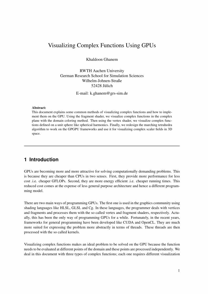
• For each point of the domain complex plane z, compute w = f(z) and then color z with thecolor of w.

The result of the above procedure is a colored image of the domain (see figure 1).

Figure 1: As an illustrating simple example, let us assume we want to visualize the square function z2 at onlyfour points 1,−1, i,−i. We give each of these points in Range plane a unique color. Then we computethe function values at these points and color them according to the result: f(1) = f(−1) = 1 (green), andf(i) = f(−i) = −1 (yellow). The image to the right is called color map and the one to the left is plot of z2

2.2 Choosing Color Map

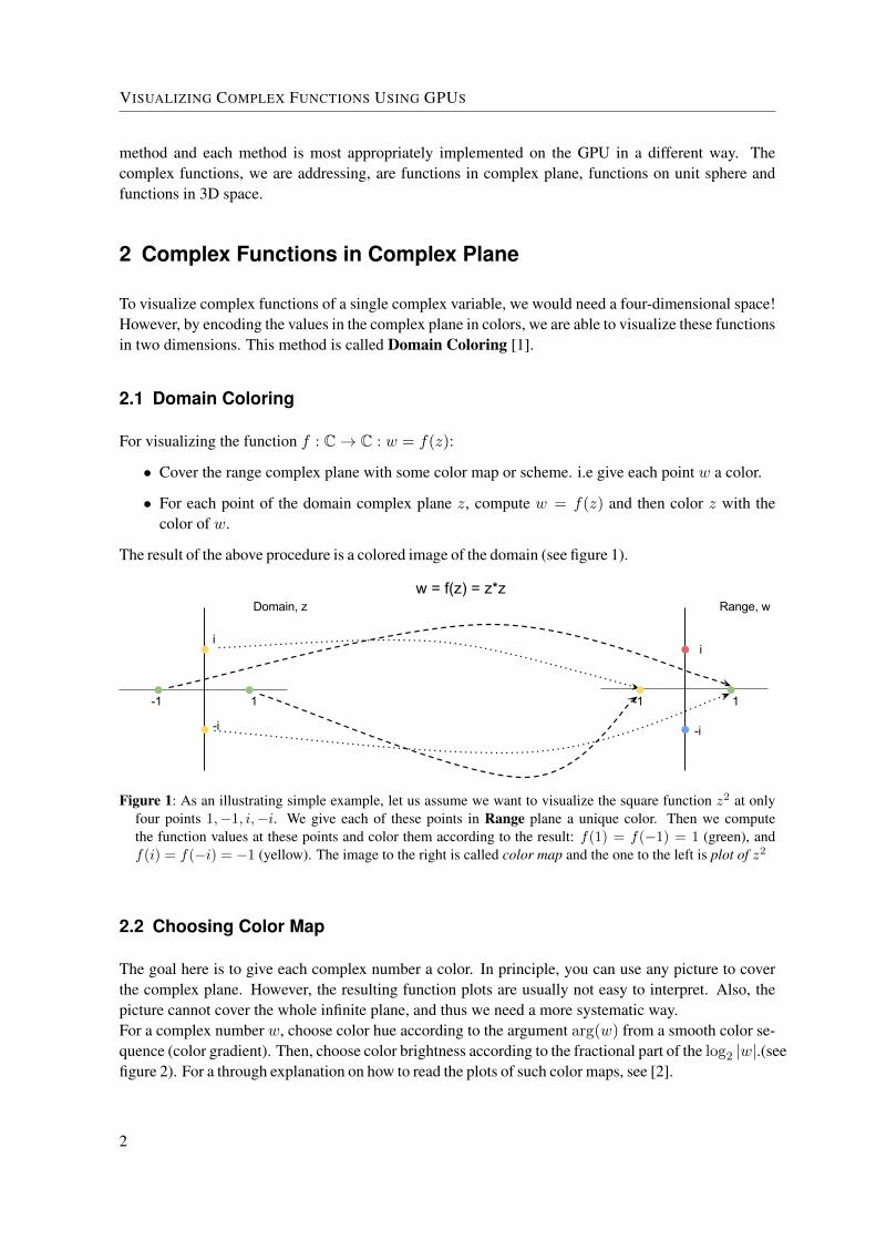
The goal here is to give each complex number a color. In principle, you can use any picture to coverthe complex plane. However, the resulting function plots are usually not easy to interpret. Also, thepicture cannot cover the whole infinite plane, and thus we need a more systematic way.For a complex number w, choose color hue according to the argument arg(w) from a smooth color se-quence (color gradient). Then, choose color brightness according to the fractional part of the log2 |w|.(seefigure 2). For a through explanation on how to read the plots of such color maps, see [2].

2

2 Complex Functions in Complex Plane

Figure 2: Two color maps differ by argument encoding. The first map interpolate between three colors; black,red and yellow. The second map spans the whole spectrum.

2.3 Using the GPU

The coloring of the domain complex plane is embarrassingly parallel as each point of the plane isprocessed independently. To utilize the GPU in this problem, we map complex points to screen pixelsand color them with a fragment shader written in some shading language. The procedure outline is asfollowing:

• Make a rectangle covering the whole screen using the graphics API , OpenGL or DirectX.

• The rectangle’s fragments will be created by the fixed functionality of the graphics pipeline.These fragments are the final pixels of the screen, because there is only one primitive and it isnot clipped.

• Fragment shader will be executed for each fragment. Inside fragment shader:

– Transform the fragment screen coordinates to a complex point z using a transformationmatrix passed from main program.

– Compute the function at that point f(z) = w.

– Determine the fragment color according to the color map at the resulting point w.

2.4 Implementation

We developed an application that visualize complex functions of a single variable. The main pro-gram is written using OpenGL graphics API and GLUT library while the fragment shader is writtenin GLSL shading language. The application takes as input a list of complex functions expressedwith common mathematical symbols. Function expressions are parsed and translated into appro-priate shader calls and operations using a lexical analyzer and a parser generated by lex and yacctools.

3

VISUALIZING COMPLEX FUNCTIONS USING GPUS

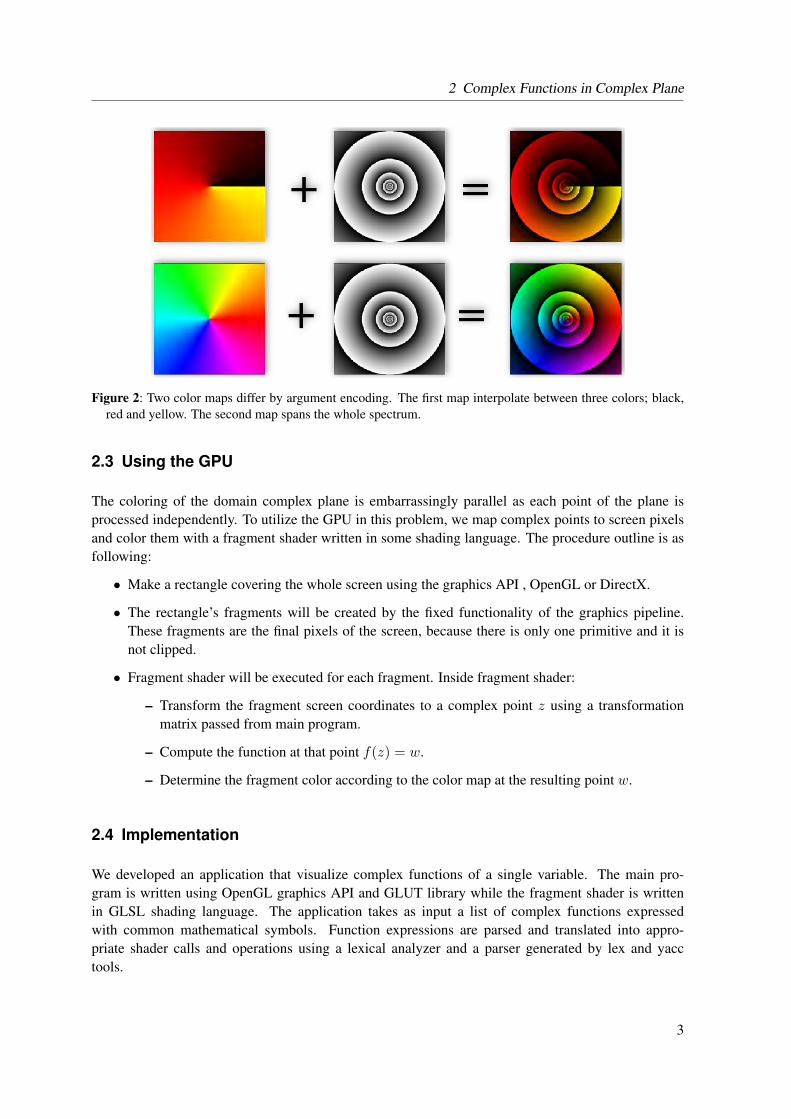
Figure 3: Plots of some complex functions generated using our domain coloring program:(z − 2)2(z + 1− 2i)(z + 2 + 2i)/z3 (left), sin(z) (center), log(z) (right).

3 Complex Functions on Unit Sphere

The second class of complex functions we address is functions defined on a unit sphere f : [0, π] ×[0, 2π) → C : f(θ, ϕ) = w. Although we could apply the domain coloring method to the surfaceof unit sphere, we are already visualizing in three dimensions and it is convenient to use the extradimension we have at our disposal.

• Start with a unit sphere in 3D space.

• Each point on the surface has the spherical coordinates (r, θ, ϕ).

• Deform the sphere such that for each point r = |f(θ, ϕ)|.

• Color the surface according to arg(f(θ, ϕ)) using some smooth color sequence as we did indomain coloring method 2.1.

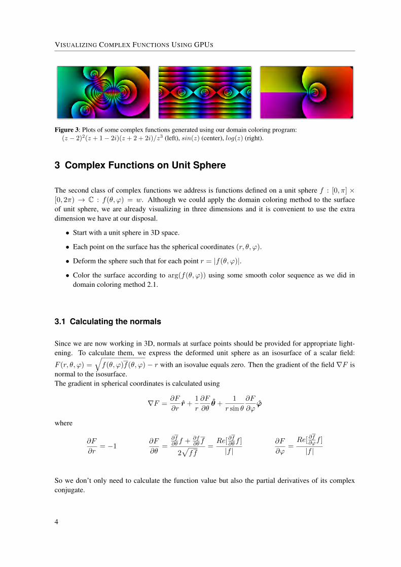
3.1 Calculating the normals

Since we are now working in 3D, normals at surface points should be provided for appropriate light-ening. To calculate them, we express the deformed unit sphere as an isosurface of a scalar field:

F (r, θ, ϕ) =√f(θ, ϕ)f(θ, ϕ) − r with an isovalue equals zero. Then the gradient of the field ∇F is

normal to the isosurface.The gradient in spherical coordinates is calculated using

∇F =∂F

∂rr̂ +

1

r

∂F

∂θθ̂ +

1

r sin θ

∂F

∂ϕϕ̂

where

∂F

∂r= −1 ∂F

∂θ=

∂f∂θ f + ∂f

∂θ f

2√ff

=Re[∂f∂θ f ]

|f |∂F

∂ϕ=Re[ ∂f∂ϕf ]

|f |

So we don’t only need to calculate the function value but also the partial derivatives of its complexconjugate.

4

4 Complex Functions in 3D

3.2 Using the GPU

We generate a unit sphere (vertices and triangles). Then, using a vertex shader, each vertex of thesphere is modified independently. Inside the vertex shader:

• Retrieve vertex’s angles (θ, ϕ)

• Compute function value f(θ, ϕ)

• Modify vertex coordinates such that r = |f(θ, ϕ)|

• Modify vertex color according to arg(f(θ, ϕ)) using some smooth color sequence.

• Compute partial derivatives of the function and use them to compute the gradient vector.

• Modify vertex normal such that it points in the direction of the gradient.

3.3 Implementation

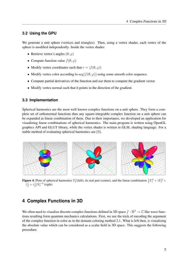
Spherical harmonics are the most well known complex functions on a unit sphere. They form a com-plete set of orthonormal functions thus any square-integrable complex function on a unit sphere canbe expanded as linear combination of them. Due to their importance, we developed an application forvisualizing linear combinations of spherical harmonics. The main program is written using OpenGLgraphics API and GLUT library, while the vertex shader is written in GLSL shading language. For astable method of evaluating spherical harmonics see [3].

Figure 4: Plots of spherical harmonics Y 13 (left), its real part (center), and the linear combination 1

2Y01 + iY 3

5 +( 12 + i 12 )Y

−37 (right)

4 Complex Functions in 3D

We often need to visualize discrete complex functions defined in 3D space f : R3 → C like wave func-tions resulting form quantum mechanics calculations. First, we use the trick of encoding the argumentof the complex function in color as in the domain coloring method 2.1. What is left then, is visualisingthe absolute value which can be considered as a scalar field in 3D space. This suggests the followingprocedure:

5

VISUALIZING COMPLEX FUNCTIONS USING GPUS

• Specify one absolute value to visualize.

• Calculate an isosurface of the absolute value using marching tetrahedra.

• Color the isosurface according to the argument using some smooth color sequence.

• If necessary, change the isovalue and repeat process to gain more info.

4.1 Marching Tetrahedra

Marching Tetrahedra is an isosurface extraction algorithm. Given a 3D scalar field, it finds the surfaceon which the field has a constant value, the isovalue. The key idea of marching tetrahedra is noting thatisosurface of a volume is the union of the isosurfaces of its components.

The field values are given at the points of a mesh. Any mesh is naturally divided into mesh cells. In thisdocument, we consider structured meshes with parallelepiped cells (usually cubes). We could take themesh cell as our building block and find the isosurface of each mesh cell independently and then collectthem to form the final isosurface. This would be called Marching Cubes Algorithm[4, 5]. Marchingcubes suffer from some ambiguities in finding the isosurface of a mesh cell. These ambiguities are notpresent in marching tetrahedra.

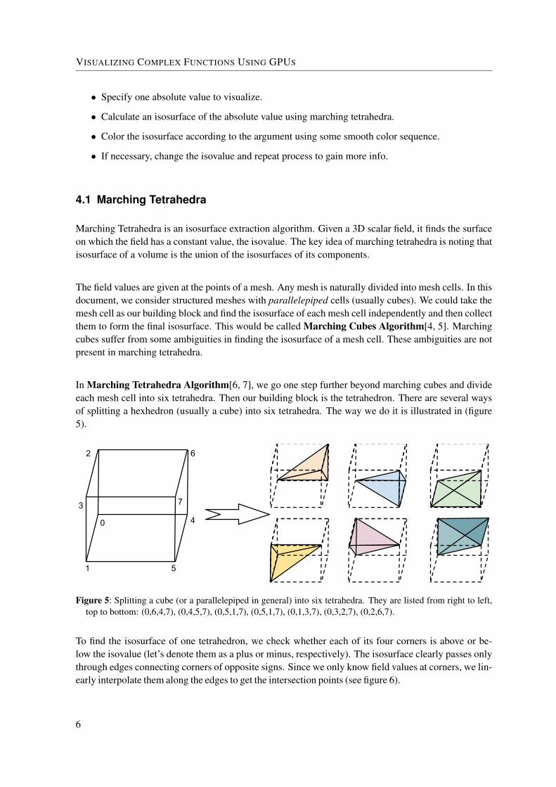
In Marching Tetrahedra Algorithm[6, 7], we go one step further beyond marching cubes and divideeach mesh cell into six tetrahedra. Then our building block is the tetrahedron. There are several waysof splitting a hexhedron (usually a cube) into six tetrahedra. The way we do it is illustrated in (figure5).

Figure 5: Splitting a cube (or a parallelepiped in general) into six tetrahedra. They are listed from right to left,top to bottom: (0,6,4,7), (0,4,5,7), (0,5,1,7), (0,5,1,7), (0,1,3,7), (0,3,2,7), (0,2,6,7).

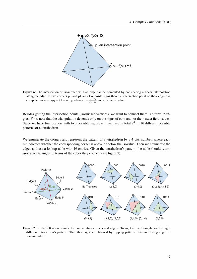
To find the isosurface of one tetrahedron, we check whether each of its four corners is above or be-low the isovalue (let’s denote them as a plus or minus, respectively). The isosurface clearly passes onlythrough edges connecting corners of opposite signs. Since we only know field values at corners, we lin-early interpolate them along the edges to get the intersection points (see figure 6).

6

4 Complex Functions in 3D

Figure 6: The intersection of isosurface with an edge can be computed by considering a linear interpolationalong the edge. If two corners p0 and p1 are of opposite signs then the intersection point on their edge p iscomputed as p = αp1 + (1− α)p0 where α = c−f0

f1−f0and c is the isovalue.

Besides getting the intersection points (isosurface vertices), we want to connect them. i.e form trian-gles. First, note that the triangulation depends only on the signs of corners, not their exact field values.Since we have four corners with two possible signs each, we have in total 24 = 16 different possiblepatterns of a tetrahedron.

We enumerate the corners and represent the pattern of a tetrahedron by a 4-bits number, where eachbit indicates whether the corresponding corner is above or below the isovalue. Then we enumerate theedges and use a lookup table with 16 entries. Given the tetrahedron’s pattern, the table should returnisosurface triangles in terms of the edges they connect (see figure 7).

Figure 7: To the left is our choice for enumerating corners and edges. To right is the triangulation for eightdifferent tetrahedron’s pattern. The other eight are obtained by flipping patterns’ bits and listing edges inreverse order.

7

VISUALIZING COMPLEX FUNCTIONS USING GPUS

4.2 Avoiding Duplicate Isosurface Vertices

We note in the original marching tetrahedra, that isosurface vertices (intersection points) lying on edgesshared between adjacent tetrahedra are duplicated. This a disadvantage for two reasons. First, it leadsto unnecessary storage of repeated vertices e.g. a vertex on the diagonal of a mesh cell would be re-peated six times. Second, if the generated surface is to be processed later or used for some calculations,then this could produce artifacts due to round-off errors. To avoid this duplication, we split the algo-rithm into two stages: Generating Vertices and Generating Triangles.

In the Generating Vertices stage, we loop over all edges. For each edge, check whether it is cut bythe isosurface (by checking whether the two end mesh points are of opposite signs). If so, calculatethe intersection point (isosurface vertex). Then store the vertex in a hash table indexed by some edge id.

In the Generating Triangles stage, we loop over all mesh cells. For each mesh cell, process all sixtetrahedra. For each tetrahedron, calculate its pattern. Using the tetrahedron’s pattern, get its triangu-lation. Generate triangles using pointers to vertices (not vertices directly). Get vertices’ pointers bylooking up edge-vertex hash table generated in the previous stage.

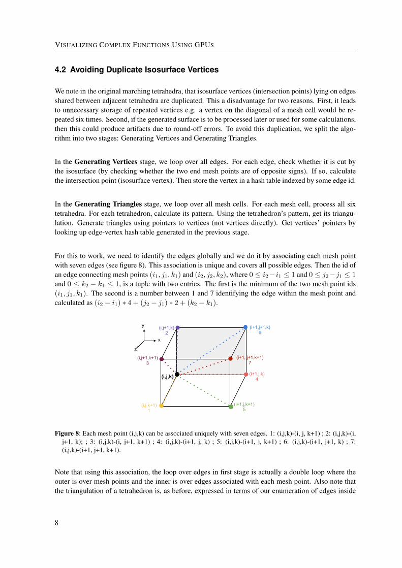
For this to work, we need to identify the edges globally and we do it by associating each mesh pointwith seven edges (see figure 8). This association is unique and covers all possible edges. Then the id ofan edge connecting mesh points (i1, j1, k1) and (i2, j2, k2), where 0 ≤ i2− i1 ≤ 1 and 0 ≤ j2−j1 ≤ 1

and 0 ≤ k2 − k1 ≤ 1, is a tuple with two entries. The first is the minimum of the two mesh point ids(i1, j1, k1). The second is a number between 1 and 7 identifying the edge within the mesh point andcalculated as (i2 − i1) ∗ 4 + (j2 − j1) ∗ 2 + (k2 − k1).

Figure 8: Each mesh point (i,j,k) can be associated uniquely with seven edges. 1: (i,j,k)-(i, j, k+1) ; 2: (i,j,k)-(i,j+1, k); ; 3: (i,j,k)-(i, j+1, k+1) ; 4: (i,j,k)-(i+1, j, k) ; 5: (i,j,k)-(i+1, j, k+1) ; 6: (i,j,k)-(i+1, j+1, k) ; 7:(i,j,k)-(i+1, j+1, k+1).

Note that using this association, the loop over edges in first stage is actually a double loop where theouter is over mesh points and the inner is over edges associated with each mesh point. Also note thatthe triangulation of a tetrahedron is, as before, expressed in terms of our enumeration of edges inside

8

4 Complex Functions in 3D

the tetrahedra (see figure 7). So a mapping from the local edge enumeration to global edge ids shouldbe done before retrieving vertices’ pointers form the hash table.

4.3 Using the GPU

Unlike the previous two visualization methods, domain coloring and sphere deformation, we won’t usea shading language but rather a GPGPU language like OpenCL or CUDA. Although it is possible toimplement the marching tetrahedra on vertex or fragment shaders (see [8, 9, 10]), it is more convenientto express the problem more abstractly using GPGPU. There are implementations of marching cubeson OpenCL and CUDA (see [11, 12]), but to our knowledge, there is no public implementation ofmarching tetrahedra using GPGPU yet.

We go along the same line of thought as in the last algorithm and separate generating vertices fromtriangles. First a collection of threads, one for each mesh point, is created. Each of these threads runs akernel that would generate vertices lying on edges associated with the corresponding mesh point. Thenanother collection of threads is created, one for each mesh cell. Each of these threads would generatethe triangles of tetrahedra associated with the corresponding mesh cell.

There are two main complications on the GPU. First, there is no dynamic memory allocation. So allmemory allocation and deallocation should be done before or after the computation but not during it.One solution is to allocate memory for every potential vertex. However, this is impractical, as it wouldneed (7 vertices per mesh point× 3 coordinates per vertex) = 21 times the storage needed for the scalarfield. A similar argument goes for the triangles.Second, the threads should work independently and write data to distinct memory locations. So eachthread should know where to write its results before starting the computation.Circumventing these problems is done by splitting each stage into yet another three stages. First, wecount the number of vertices that would be generated per mesh point. Second, a prefix-scan is doneto get the number of generated vertices and a list of addresses for storing the vertices associated witheach mesh point. Finally, the necessary memory is allocated and vertices are generated and stored intheir appropriate locations. Triangle generation is also split into three stages similarly. This method ishighly inspired by [11, 12].

Generating Vertices

1. Allocate necessary memory on GPU for array mpVertsNum.mpVertsNum: An array of bytes. Its size equals the total number of mesh points. ElementmpVertsNum[mp] contains the number of vertices associated with mesh point mp.

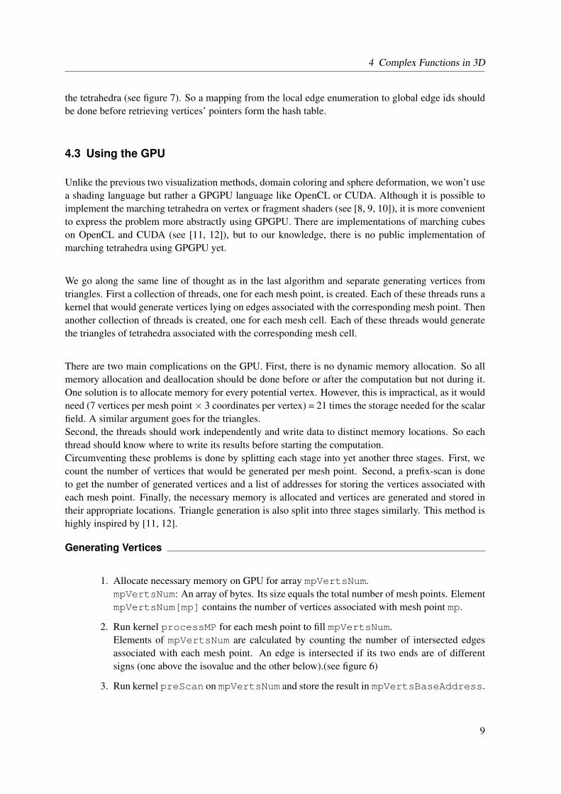
2. Run kernel processMP for each mesh point to fill mpVertsNum.Elements of mpVertsNum are calculated by counting the number of intersected edgesassociated with each mesh point. An edge is intersected if its two ends are of differentsigns (one above the isovalue and the other below).(see figure 6)

3. Run kernel preScan on mpVertsNum and store the result in mpVertsBaseAddress.

9

VISUALIZING COMPLEX FUNCTIONS USING GPUS

mpVertsBaseAddress: An array of integers. Its size equals the total number of meshpoints. Element mpVertsBaseAddress[mp] indicates where vertices, associated withmesh point mp, should be stored in the vertex array. It is computed as a prefix-scan ofarray mpVertsNum. So element mpVertsBaseAddress[mp] contains the sum ofmpVertsNum elements up to and excluding mp. There is an efficient implementation ofprefix-scan algorithm on GPU (see [13]).

4. Allocate memory on GPU for array verts of size vertsNum.vertsNum: An integer containing the number of generated vertices.It is computed as the sum of the last entries of mpVertsNum and its prefix-scanned ver-sion mpVertsBaseAddress.verts: An array of floats. Its size equals three times vertsNum. It stores the coor-dinates of the generated vertices. The three coordinates of each vertex are stored con-secutively. The vertices associated with each mesh point are stored consecutively from3*mpVertsBaseAddress[mp] till 3*mpVertsBaseAddress[mp+1]. Verticesof a mesh point are ordered according to the local ordering of the edges they lay on (seefigure 8).

5. Run kernel generateVerts for each mesh point to fill verts.Vertex coordinates are computed as linear interpolation (see figure 6).

Generating Triangles

1. Allocate necessary memory on GPU for array mcTriangsNum.

2. Run kernel processMC for each mesh point to fill array mcTriangsNum.

3. Run the kernel preScan on array mcTriangsNum and store the result in arraymcTriangsBaseAddress.

4. Allocate memory on GPU for array triangs.

5. Run kernel generateTriangs for each mesh cell to fill array triangs.

The semantics are very similar to Generating Vertices; Just replace mesh points with meshcells, edges with tetrahedra and vertices with triangles.One complication in the final step is getting the addresses of vertices which will be used in form-ing triangles. Triangles are expressed in terms of the edges on which their vertices lie. So theproblem reduces to knowing where the vertex of a certain edge is stored.If mp is lowest numbered mesh point of an edge then the vertex of that edge will be located at3*mpVertsBaseAddress[mp] in array verts with some additional shift that depends onother vertices associated with mp. To get this shift easily, we build an array mpVertsEdgeIndexwhere the bit number i of element mpVertsEdgeIndex[mp] indicates whether edge num-ber i associated with mesh point mp is intersected by the isosurface. This way, all the infor-mation needed for determining shifts of vertices associated with mesh point mp are contained inmpVertsEdgeIndex[mp]. The computation of this array is most conveniently done insidekernel processMP.

10

4 Complex Functions in 3D

4.4 More Details and Optimization

In the previous description, we omitted several aspects of the method to make the presentation moreclear. They are explained here:

• Many subtask like splitting the mesh cell into tetrahedra, getting triangles from tetrahedra pat-tern, getting shifts from mpEdgeIndex, etc. can be done using look-up tables. These look-uptables should be stored in the constant memory of GPU which is basically a small fast read-onlymemory.

• Considerable speed-up can be obtained by considering only mesh points that actually have anon-zero number of associated vertices and only mesh cells that actually generate triangles. Thisrequires building yet another array for knowing which mesh points are ’active’. Note also thatby associating each mesh cell with its lowest numbered mesh point, a mesh cell can be skippedif that mesh point is not active.

• Kernels processMP and processMC can be combined for speed-up. This because every meshcell can be associated with its lowest numbered mesh point and then both kernels need to readthe same memory locations. Thus, combining them saves repeated memory accesses.

• For getting the normals, central difference formula can be used to get normals at mesh points.This could be done outside the marching tetrahedra algorithm. The normals at isosurface verticesare then computed in the same way as the coordinates .i.e. as a linear interpolation and thiscomputation can be incorporated inside kernel generateVers.

4.5 Implementation

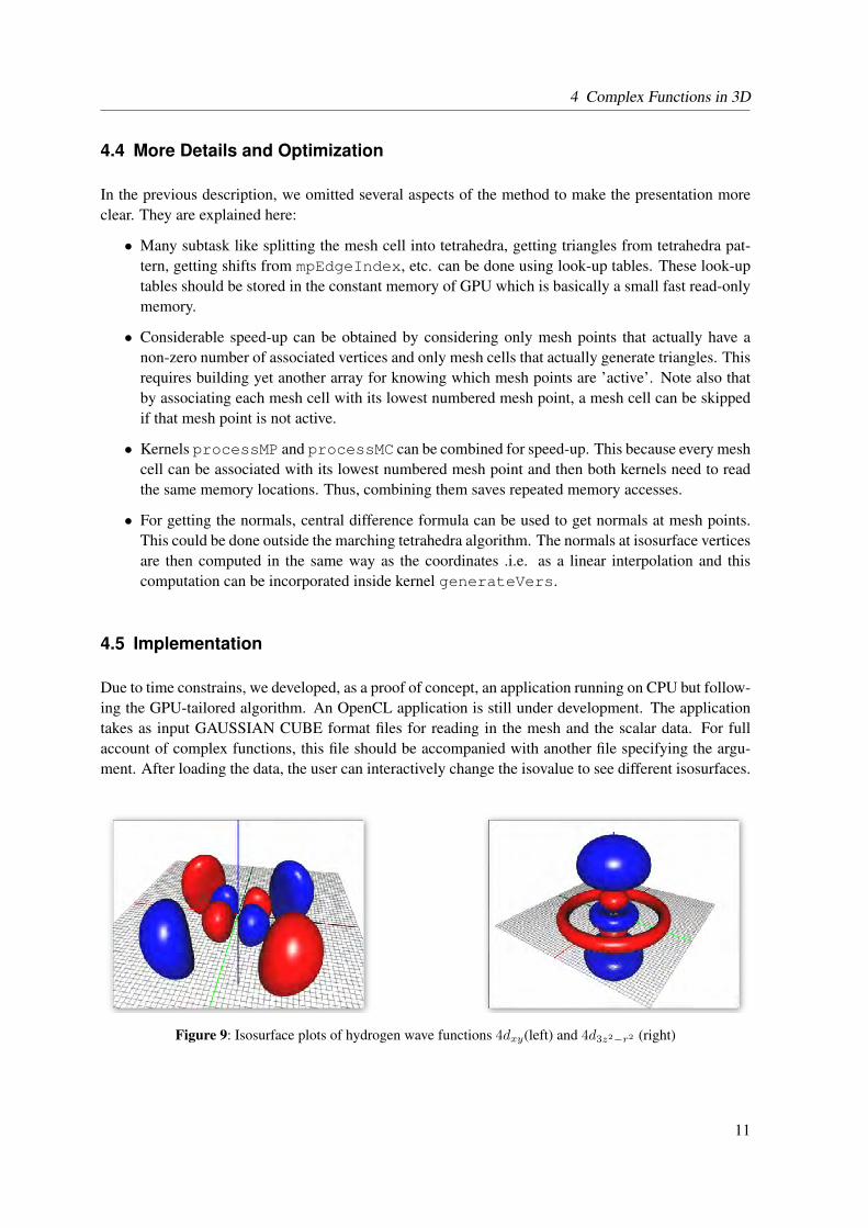
Due to time constrains, we developed, as a proof of concept, an application running on CPU but follow-ing the GPU-tailored algorithm. An OpenCL application is still under development. The applicationtakes as input GAUSSIAN CUBE format files for reading in the mesh and the scalar data. For fullaccount of complex functions, this file should be accompanied with another file specifying the argu-ment. After loading the data, the user can interactively change the isovalue to see different isosurfaces.

Figure 9: Isosurface plots of hydrogen wave functions 4dxy(left) and 4d3z2−r2 (right)

11

VISUALIZING COMPLEX FUNCTIONS USING GPUS

5 Summary

We described how to visualize three different classes of complex functions using the GPU. First, weexplained how to visualize complex functions of a single complex variable using the domain coloringmethod on the fragment shader. Then, we explained how to visualize complex function defined onunit sphere by deforming that sphere and coloring it. This is done on the vertex shader. Finally, weexplained how to visualize complex functions in 3D space by extracting the isosurfaces of the absolutevalue using marching tetrahedra method and then coloring that surface. This was designed to work ona GPGPU framework.

6 Acknowledgements

I would like to thank my supervisor Prof. Erik Koch for bringing this interesting program to my atten-tion to and for providing the necessary knowledge and advice to finish the project successfully. I wouldlike also to thank German Research School for Simulation Sciences for sponsoring my project. Last butnot least, I would like to thank Jülich Supercomputing Center staff and in particular Mr. Mathias Winkelfor organising the program and making it a unique experience.

References1. Wikipedia contributors. Domain Coloring [Internet]. Wikipedia, The Free Encyclopedia [updated 2012 September 20;

cited 2012 Oct 07]. Available from: http://en.wikipedia.org/wiki/Domain_coloring2. Lundmark M. Visualizing complex analytic functions using domain coloring [internet]. 2004 May [cited 2012 Oct 07].

Available from: www.mai.liu.se/ halun/complex/domain_coloring-unicode.html3. Press WH, Teukolsky SA, Vetterling WT, Flannery BP. Numerical Recipes, The Art of Scientific Computing. 3rd ed.

New York: Cambridge University Press;2007. Chapter 6, Special Functions; p.292-295.4. Lorensen WE, Cline HE. Marching cubes: A high resolution 3D surface construction algorithm. SIGGRAPH Comput.

Graph. 1987 Aug;21(4):163-169.5. Bourke P. Polygonising a scalar field [Internet]. 1994 May [cited 2012 Oct 04]. Available from:

http://paulbourke.net/geometry/polygonise/6. Doi A, Koide A. An Efficient Method of Triangulating Equivalued Surfaces by using Tetrahedral Cells. IEICE Trans

Inf Syst. 1991 Jan;E74(1):214-224.7. Bourke P. Polygonising a Scalar Field Using Tetrahedrons [Internet]. 1997 Jun [cited 2012 Oct 04]. Available from:

http://paulbourke.net/geometry/polygonise/8. Reck F, Dachsbacher C, Grosso R, Greiner G, Stamminger M. Realtime isosurface extraction with graphics hardware.

Eurographics 2004 Short Presentations; 2004.9. Pascucci V. Isosurface computation made simple: Hardware acceleration, adaptive refinement and tetrahedral stripping.

Proceedings of IEEE TCVG Symposium on Visualization; 2004. p. 293–300.10. Klein T, Stegmaier S, Ertl T. Hardware-accelerated Reconstruction of Polygonal Isosurface Representations on Un-

structured Grids. Proceedings of Pacific Graphics ’04; 2004. p.186–195.11. NVIDIA CUDA SDK - Physically-Based Simulation - Marching Cubes Isosurfaces [Internet]. 2008 [updated

2009 June 15; cited 2012 Oct 05]. Available from: http://www.nvidia.com/content/cudazone/cuda_sdk/Physically-Based_Simulation.html#marchingCubes

12. NVIDIA OpenCL SDK Code Samples -OpenCL Marching Cubes Isosurfaces [Internet]. [cited 2012 Oct 05]. Availablefrom: http://developer.download.nvidia.com/compute/cuda/4_2/rel/sdk/website/OpenCL/html/samples.html

13. Harris M, Sengupta S, Owens JD. GPU Gems 3. Addison-Wesley Professional; 2007. Chapter 39. Parallel Prefix Sum(Scan) with CUDA.

12