Visualizing Dynamic Metrics with ProfilingBlueprints

Alexandre Bergel1, Romain Robbes1, and Walter Binder2

1 Pleiad Lab, DCC, University of Chile, Santiago, Chilehttp://bergel.eu http://www.dcc.uchile.cl/∼rrobbes

2 University of Lugano, Switzerlandhttp://www.inf.usi.ch/faculty/binder

In Proceedings of the 48th International Conference on Objects, Models,Components, Patterns (TOOLS EUROPE’10), LNCS Springer Verlag

Abstract. While traditional approaches to code profiling help locateperformance bottlenecks, they offer only limited support for removingthese bottlenecks. The main reason is the lack of visual and detailedruntime information to identify and eliminate computation redundancy.We provide two profiling blueprints which help identify and remove per-formance bottlenecks. The structural distribution blueprint graphicallyrepresents the CPU consumption share for each method and class of anapplication. The behavioral distribution blueprint depicts the distributionof CPU consumption along method invocations, and hints at methodcandidates for caching optimizations. These two blueprints helped usto significantly optimize Mondrian, an open source visualization engine.Our implementation is freely available for the Pharo development envi-ronment and has been evaluated in a number of different scenarios.

1 Introduction

Even though computing resources are abundant, execution optimization throughcode profiling remains an important software development activity. A CPU timeprofiler is a crucial tool to identify bottlenecks – program elements that take alarge part of the execution time. Today, it is inconceivable to ship a programmingenvironment without a code profiler included or provided by a third party.

However, when we retrospectively look at the history of code profiler tools, wesee that tool usability and profiling overhead reduction have steadily improved,but that the set of offered abstractions has remained constant. For instance,gprof, which appeared in 1982, offers a number of textual reports focussed on“how much time was spent executing directly in each function” and call graphs1.JProfiler essentially produces the same output, using a graphical rendering in-stead of a textual one2. Most of the research conducted in the field of code pro-filing focus on reducing the overhead triggered by the code instrumentation and1 http://sourceware.org/binutils/docs/gprof/Output.html#Output2 http://www.ej-technologies.com/products/jprofiler/screenshots.html

observation. On the other hand, the abstractions used to profile object-orientedapplications are very close to the ones for procedural applications.

The contribution of this paper is to apply some visualizations that have beenpreviously used in static software analysis to display dynamic metric for profil-ing purposes. We propose a visual mechanism for rendering dynamic informationthat effectively enables comparison of different metrics related to a program ex-ecution. Structural distribution blueprint and behavioral distribution blueprintare two visualizations intended to identify bottlenecks and propose hints on howto remove them. The first blueprint represents the distribution of the CPU ef-fort along the program structure. The second blueprint directs the distributionalong method invocations and identifies methods prone to one class of optimiza-tion, namely caching. The work presented in this paper aims at complementingexisting profilers with new visualizations that help specific optimization tasks.

The results presented in this paper were realizing using Pharo3, an open-source Smalltalk-dialect programming language. Nothing in the visualizationswe propose prevents one from using them in a different setting.

We apply our techniques to the visualization framework Mondrian4 [MGL06],our running example. We first describe our blueprints (Section 2). Subsequently,we identify and implement opportunities for optimization in Mondrian (Section3). We then review related work (Section 4) and conclude (Section 5).

2 Profiling Blueprints

2.1 Profiling blueprint in a nutshell

Time profiling blueprints are graphical representations meant to help program-mers (i) assess the time distribution and (ii) identify bottlenecks and give hintson how to remove them for a given program execution. The essence of profilingblueprints is to enable a better comparison of elements constituting the programstructure and behavior. To render information, these blueprints use a graphmetaphor, composed of nodes and edges.

The size of a node hints at its importance in the execution. In the case thatnodes represent methods, a large node may say that the program executionspends “a lot of time” in this method. The expression “a lot of time” is thenquantified by visually comparing the height and/or the width of the node againstother nodes.

Color is used to either transmit a boolean property (e.g., a gray node rep-resents a method that always returns the same value) or a metric (e.g., a colorgradient is mapped to the number of times a method has been invoked).

We propose two blueprints that help identify opportunities for code opti-mization. They provide hints to programmers to refactor their program alongthe following two principles: (i) make often-used methods faster and (ii) call slowmethods less often. The metrics we adopted in this paper help finding methods3 http://www.pharo-project.org/home4 http://www.moosetechnology.org/tools/mondrian

2

that are either unlikely to perform a side effect or return always the same result,good candidates for simple caching optimizations.

2.2 Polymetric views

width property

heightproperty

colorproperty

edge width and color properties

X property

Yproperty

Fig. 1. Principle of polymetric view.

The blueprints we propose are graphically rendered as polymetric views [LD03].A polymetric view is a lightweight software visualization enriched with softwaremetrics. It has been successfully used to provide “software maps” intended tohelp software comprehension and visualization. Figure 1 depicts the general as-pect of a polymetric view.

Given two-dimensional nodes representing entities, we can map up to 5 met-rics on the node characteristics: position (X and Y ), size (width and height),and color:

– Position. The X and Y coordinates of the position of a node may reflect twomeasurements.

– Size. The width and height of a node can render two measurements. Wefollow the intuitive notion that the wider and the higher the node, the largerthe associated metric.

– Color. The color interval between white and black may render one mea-surement. The convention that is usually adopted [GL04] is that the higherthe measurement, the darker the node. Thus light gray represents a smallermeasurement than dark gray.

Edges may also render properties along a number of dimensions (width, color,direction, etc.). However, for the purpose of this work, all edges are identical.

2.3 Structural distribution blueprint

The execution of an object-oriented program yields a large amount of informa-tion [DLB04] (e.g., number of objects created at runtime, total execution time ofa method). Unfortunately, all these dimensions cannot be visually rendered in a

3

meaningful fashion. The structural distribution blueprint displays a selected num-ber of metrics indicating the distribution of the execution time along the staticstructure of a program (i.e., classes, methods and class hierarchy). Table 1 givesthe specification of the structural distribution blueprint. The blueprint rendersa program in terms of classes, methods and inheritance relations. Each methodrepresentation exhibits its corresponding CPU time profiling information alongthree metrics:

– number of different receivers: amount of different object receivers the methodhas been invoked on. Due to implementation limitations, this is at the mo-ment a lower bound estimate.

– total execution time of a method : time for which a call frame correspondingto the method is present on the stack at runtime. The precision depends onthe underlining profiler used to collect runtime information.

– number of executions: number of times the method has been executed, in-dependently of the object receiver.

Actual metric values, and additional information, are accessible through acontextual popup window.

Structural distribution blueprint

Scope full system execution time

Edge class inheritance (upper is superclass of below)Layout tree layout for outer nodes and gridlayout for inner nodes

(inner nodes are ordered by increasing height)Metric scale linear (except for node width)Node outer node is a class, an inner node is a method

Inner node color Number of different receiversInner node height total execution time of a methodInner node width number of executions (logarithmic scale)

Example Figure 2

Table 1. Specification of the structural distribution blueprint

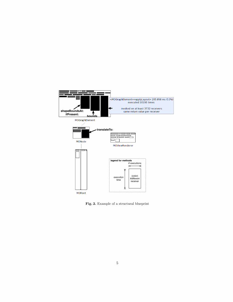
Example. Troughout this paper, we use the graph visualization framework Mon-drian as a case study. The blueprints described in this paper are also renderedusing Mondrian. An example of the structural distribution blueprint is given inFigure 2. Four classes are represented: MOGraphElement, MOViewRenderer, MON-ode and MORoot. This figure is a small part of a bigger picture obtained byevaluating the following code snippet, which renders a simple visualization of100 nodes, each containing 100 nodes:

ProfilingPackageSpyviewProfiling: [

| view |view := MOViewRenderer new.

4

legend for methods

(color)#different receiver

# executions

execution time

bounds

translateTo:

shapeBoundsAt:ifPresent:

Fig. 2. Example of a structural blueprint

5

view nodes: (1 to: 100)forEach: [:each | view nodes: (1 to: 100)].

view root applyLayout ]inPackage: ’Mondrian’

The code being profiled is indicated using a bold font in the example sourcecode. The profiling is realized from the perspective of one package, Mondrian inour case. MOGraphElement inherits from MONode, MORoot from MOGraphElement,and MOViewRenderer from Object. Since Object does not belong to Mondrian (butto the Kernel package), it is not rendered in the blueprint.

The height of a method node is proportional to the total execution timetaken by the method (e.g., 53% of the code execution is spent in the methodapplyLayout and 38% in bounds). The width is proportional to the number of timesthe method has been executed. A logarithmic scale is used. The method nodecolor represents the number of different objects this method has been executedon (more than 3 732). The scope of the blueprint is global, which means thatthe darkest method corresponds to the method that has been executed on thegreatest number of object receivers, system-wide.

Moving the mouse over a method node pops up additional contextual infor-mation. In the example, the contextual window says that the method applyLayout

defined in the class MOGraphElement has been executed 10 100 times, and hasbeen executed on more than 3 732 distinct receiver objects (i.e., instances ofMOGraphElement or one of its subclasses). It is also indicated that this methodreturns always the same value for a given object receiver. While the blueprintemphasizes the three metrics indicated above, the contextual information pro-vides useful data when one wants to know more about a particular method.

Within a class, methods are ordered along their height. This helps quicklyspot the amount of costly methods. For example, it is clear that among MO-

GraphElement’s methods, 3 are dominating with respect to execution time.

Interpretation. Classes represented in Figure 2 illustrate part of a scenariothat totals 11 classes. Among the 111 classes that define Mondrian, these 11classes are the only classes involved in the code snippet execution given above.Only classes that are covered by the execution, even partially, are depicted inthe blueprint.

MOGraphElement contains “many large and dark” methods. This indicatesthat this class is central to the code snippet execution: these large and blackmethods consume a lot of CPU time and are invoked on many different instances.Almost all of MOGraphElement’s methods are executed a large number of times: inthe visualization, they are quite wide compared to methods in other classes. Formost of them, this is not a problem because they are thin and horizontal: evenif these methods are executed many times, they do not consume CPU time. Onthe left of applyLayout stands the bounds method. This method takes 38% of theCPU time and is invoked 70 201 times on more than 3 732 object receivers. Thethird costliest method on MOGraphElement, shapeBoundsAt:ifPresent: takes 33% ofthe CPU time. MONode contains a black and relatively large method: MONode>>

6

translateTo: consumes 22% of the total CPU time. The method has been invoked10 100 times on at least 3 732 receivers.

Comparing to MOGraphElement, we find that classes are not involved in thecomputation as much. The representation of MOViewRenderer quickly says thatits methods are invoked a few times without consuming much CPU. Moreover,methods are white, which tells that they are invoked on few instances only. Thecontextual information obtained by moving the mouse over the methods revealsthat these methods are executed on a unique receiver. This is not surprisingsince only one instance of MOViewRenderer is created in the code example givenabove.

MORoot also does not seem to be the cause of a bottleneck at runtime. Thefew methods of this class are not frequently executed since they are relativelynarrow. MORoot also defines a method applyLayout. This method is the tall, thinand white method. The contextual information reveals that this method is ex-ecuted once and on one object only. It consumes 97% of the CPU time. Themethod MORoot>> applyLayout invokes MOGraphElement>> applyLayout on each ofthe nodes. The relation between these two applyLayout methods is indicated by afly-by-highlighting (not represented in the picture) and the behavioral distribu-tion blueprint, described below.

All in all, a large piece of the total CPU time is distributed over four meth-ods: MONode>> translateTo: (24%), MOGraphElement>> bounds (32%), MOGraphEle-

ment>> shapeBoundsAt:ifPresent: (33%), MOGraphElement>> applyLayout (53%). Notethat at this stage, we cannot say that the CPU time share of these three meth-ods is the sum of their individual share. We have 24 + 32 + 33 + 53 = 142.This indicates that some of these methods call each other since their sum cannotexceed 100%.

2.4 Behavioral distribution blueprint

In a pure object-oriented setting, computation is solely performed through mes-sage sending between objects. The CPU time consumption is distributed alongmethod executions. Assessing the runtime distribution along method invoca-tions complements the structural distribution described in the previous section.To reflect this profiling along method invocations, we provide the behavioraldistribution blueprint. Table 2 gives the specification of the figure.

The goal of this blueprint is to assess runtime information alongside methodcall invocations. It is intended to find optimization opportunities, which may betackled with caching. In addition to the metrics such as the number of calls andexecution time, we also show whether a given method returns constant values,and whether it is likely to perform a side effect or not. As shown later, thisinformation is helpful to identify a class of bottlenecks.

Classes do not appear on this blueprint. Methods are represented by nodesand invocations by directed edges. The blueprint uses the two metrics describedin the previous blueprint for the width and height of a method. In addition tothe shape, node color indicates a property:

7

– the gray color indicates methods that return self, the default return value.When no return value is specified in Pharo, the object receiver is returned.This corresponds to void methods in a statically typed language. No resultis expected from the method, strongly suggesting that the method operatesvia side effects.

– the yellow color (which appears as light gray on a black and white printout)indicates methods that are constant on their return value, this value beingdifferent from self.

– other methods are white.

A tree layout is used to order methods, with upper methods calling lowermethods. We illustrates this blueprint on the MOGraphElement>> bounds methodthat we previously saw, a candidate for optimization.

Behavioral distribution blueprint

Scope all methods directly or indirectly invoked for a givenstarting method

Edge method invocation (upper methods invoke lower ones)Layout tree layoutMetric scale linear (except for node width)Nodes methods

Node color gray: return always self; yellow: same return value perobject receiver; white: remaining methods

Node height total execution timeNode width number of execution (logarithmic scale)

Example Figure 3

Table 2. Specification of the behavioral distribution blueprint

Example. In the previous blueprint (Figure 2), right-clicking on the methodMORoot>> applyLayout opens a behavioral distribution blueprint for this method.The complete picture is given in Figure 3. The picture has to be read top-down. Methods in this blueprint have the same dimensions as in the behavioralblueprint. We recognize the tall and thin MORoot>> applyLayout at the top. Allmethods in Figure 3 are therefore invoked directly or indirectly by this apply-

Layout. MORoot>> applyLayout invokes 3 methods, including MOGraphElement>>

applyLayout (labelled in the figure). MOGraphElement>> applyLayout calls MOAb-

stractLayout>> applyOn:, and both of these are called by MORoot>> applyLayout.

Interpretation. As the first blueprint revealed, bounds, applyLayout, shapeBound-

sAt:ifPresent:, translateTo: are expensive in terms of CPU time consumption. Thebehavior blueprint highlights this fact from a different point of view, alongmethod invocations. In the following we will optimize bounds by identifying the

8

legend for methods

gray = return self

yellow = constant on return

value

# executions

execution time

m2m1

invokes m2 and m3

MOGraphElement>>applyLayout

bounds

shapeBoundsAt:ifPresent:

MONode>>translateTo:

m1 m3

MOAbstractLayout>>applyOn:

MORoot>>applyLayout

Fig. 3. Example of a behavioral blueprint

9

reason of its high cost and provide a solution to fix it. Our experience with Mon-drian tells us that this method has a surprisingly high cost. Where to start arefactoring among all potential candidates remains the programmer task. Ourblueprint only says “how it is” and not “how it should be”, however it is a richsource of indication of what’s going on at runtime.

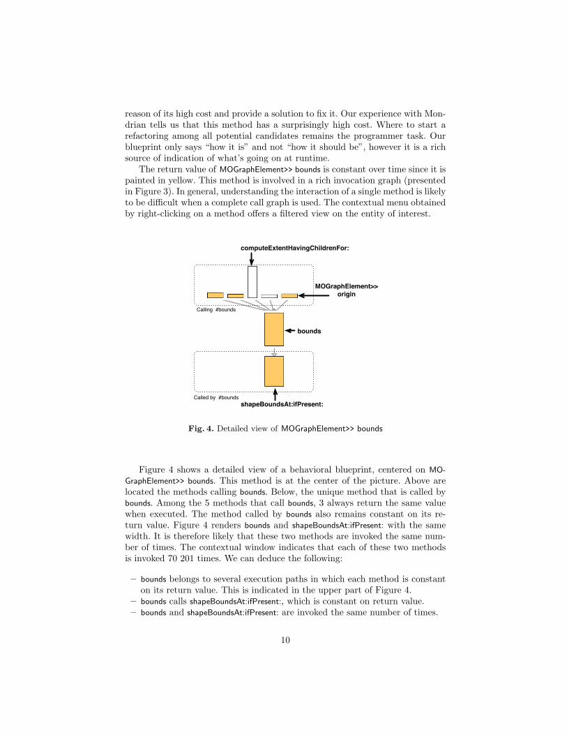
The return value of MOGraphElement>> bounds is constant over time since it ispainted in yellow. This method is involved in a rich invocation graph (presentedin Figure 3). In general, understanding the interaction of a single method is likelyto be difficult when a complete call graph is used. The contextual menu obtainedby right-clicking on a method offers a filtered view on the entity of interest.

MOGraphElement>>origin

shapeBoundsAt:ifPresent:Called by #bounds

Calling #bounds

bounds

computeExtentHavingChildrenFor:

Fig. 4. Detailed view of MOGraphElement>> bounds

Figure 4 shows a detailed view of a behavioral blueprint, centered on MO-

GraphElement>> bounds. This method is at the center of the picture. Above arelocated the methods calling bounds. Below, the unique method that is called bybounds. Among the 5 methods that call bounds, 3 always return the same valuewhen executed. The method called by bounds also remains constant on its re-turn value. Figure 4 renders bounds and shapeBoundsAt:ifPresent: with the samewidth. It is therefore likely that these two methods are invoked the same num-ber of times. The contextual window indicates that each of these two methodsis invoked 70 201 times. We can deduce the following:

– bounds belongs to several execution paths in which each method is constanton its return value. This is indicated in the upper part of Figure 4.

– bounds calls shapeBoundsAt:ifPresent:, which is constant on return value.– bounds and shapeBoundsAt:ifPresent: are invoked the same number of times.

10

The following section addresses this bottleneck by adding a cache in bounds

and unveils another bottleneck in Mondrian.

3 Optimizing Mondrian

The combination of the structural and behavioral blueprints helped us to iden-tify a number of bottlenecks in Mondrian. In this section, we address some ofthese bottlenecks by using memoization5, i.e. we cache values to avoid redundantcomputations.

3.1 Bottleneck MOGraphElement>> bounds

As we saw earlier, the behavioral blueprint on the method MOGraphElement>>

bounds reveals a number of facts about the program’s execution. These facts aregood hints that bounds will benefit from a caching mechanism since it alwaysreturns the same value and calls a method that is also constant. We inspect itssource code:

MOGraphElement>> bounds”Answer the bounds of the receiver.”| basicBounds |self shapeBoundsAt: self shape ifPresent: [ :b | ˆ b ].

basicBounds := shape computeBoundsFor: self.self shapeBoundsAt: self shape put: basicBounds.ˆ basicBounds

The code source confirms that shapeBoundsAt:ifPresent: is invoked once eachtime bounds is invoked. The method shape is also invoked at each invocation ofbounds. The contextual window obtained in the structural blueprint reveals thatthe return value of shape is constant: It is a simple variable accessor (“getter”method), so it is fast. bounds calls computeBoundsFor: and shapeBoundsAt:put: inaddition to shapeBoundsAt:ifPresent: and shape. However, they do not appear inFigure 3 and 4. This means that bounds exits before reaching computeBoundsFor:.The block [:b | ˆb], which has the effect of exiting the method, is therefore alwaysexecuted in the considered example.

We first thought that the last tree lines of bounds may be removed since theyare not executed in our scenario. However, the large number of tests in Mondrianindicate that these lines are indeed important in some scenarios although theyare not in our particular example.

We elected to upgrade bounds with a simple cache mechanism. Differenceswith the original version are indicated using a bold font. The class MOGraphEle-

ment is extended with a new instance variable, boundsCache. In addition, the cachevariable has to be reset in 5 methods related to graphical bounds manipulationof nodes, such as translating and resizing.5 http://en.wikipedia.org/wiki/Memoization

11

MOGraphElement>> bounds”Answer the bounds of the receiver.”| basicBounds |boundsCache ifNotNil: [ ˆ boundsCache ].self shapeBoundsAt: self shape ifPresent: [ :b | ˆ boundsCache := b ].

basicBounds := shape computeBoundsFor: self.self shapeBoundsAt: self shape put: basicBounds.ˆ boundsCache := basicBounds

There is no risk of concurrent accesses of boundsCache since this variable isset when the layout is being computed. This occurs before the display of thevisualization, which is done in a different thread.

Result. Adding a statement boundsCache ifNotNil: [ ˆ boundsCache ] significantlyreduces the execution time of the code given in Section 2.3. Before adding thissimple cache mechanism, the code took 430 ms to execute (on a MacBook Pro,2Gb of RAM (1067 MHz DDR3), 2.26 GHz Intel Core 2 Duo, Squeak VM4.2.1beta1U). With the cache, the same execution takes 242 ms only, whichrepresents a speedup of approximately 43%.

This gain is reflected on the overall distribution of the computational effort.Figure 5 provides two structural blueprints of the code snippet given in Sec-tion 2.3. The left blueprint has been produced before upgrading the methodMOGraphElement>> bounds. Figure 2 is a part of it. The right one has been pro-duced after upgrading bounds as described above. Many places are impacted. Weannotated the figure with the most significant changes:

– the size of the bounds method and the methods invoked by it (C) have seentheir height significantly reduced. Before the optimization, bounds used 38%of the total CPU consumption. After the optimization, its CPU use fell to5%.

– the 5 methods denoted by the circle A and B have seen their height increasedand their color darkened. The height increase illustrates the augmentationin relative CPU consumption these methods are subject to, now that bounds

has been improved.

The evolution of the behavioral blueprint is presented in Figure 6. We canclearly see the reduced size of bounds and shapeBoundsAt:ifPresent: (Circle B) andthe increase of the applyLayout method (Circle A).

3.2 Bottleneck in MONode>> displayOn:

We fixed an important bottleneck when computing bounds in Mondrian. Wepush our analysis of bounds computing a step further. We inspect the UserInterface (UI) thread of Mondrian. Most applications with a graphical user in-terface run in at least 2 threads: one for the program logic and another in chargeof receiving user events (e.g., keystrokes, mouse events) and virtual machine/OS

12

A

B

C

Upgrading MOGraphElement>>bounds

Fig. 5. Upgrading bounds has a global structural impact

B

A

Upgrading MOGraphElement>>bounds

Fig. 6. Upgrading bounds has a global behavioral impact

13

events (e.g., window refreshes). Mondrian is no exception. The blueprints pre-sented earlier focused on profiling the application logic.

legend for methods

(color)#different receiver

# executions

execution time

displayOn:

absoluteBounds

shapeBoundsAt:ifPresent:

absoluteBoundsFor:

display:on:

Fig. 7. Profiling of the UI thread in Mondrian

Step 1. Figure 7 shows the structural profiling of the UI thread for the Mon-drian script given in Section 2.3. The blueprint contains many large methods,indicating methods that received a significant CPU share. Among these, ourknowledge of Mondrian lead us to absoluteBounds. This method is very similarto bounds that we previously saw. It returns the bounds of a node using abso-lute coordinates (instead of relative). The UI thread spends most of the time inMONode>> displayOn: since it is the root of the thread’s computation.

Figure 8 shows the behavioral blueprint opened on MONode>> displayOn:. Theblueprint reveals that absoluteBounds and absoluteBoundsFor: call each other. Re-turn values of these two methods are constant as indicated by their yellow color.They are therefore good candidates for caching:

14

MONode>>displayOn:

MOGraphElement>>absoluteBoundsMOShape>>

absoluteBoundsFor:

legend for methods

gray = return self

yellow = constant on return

value

# executions

execution time

m2m1

invokes m2 and m3

m1 m3

MORectangleShape>>display:on:

Fig. 8. Profiling of the UI thread in Mondrian

15

MOGraphElement>> absoluteBounds”Answer the bounds in absolute terms (relative to the entire Canvas, not just the parent).”absoluteBoundsCache ifNotNil: [ ˆabsoluteBoundsCache ].ˆabsoluteBoundsCache := self shape absoluteBoundsFor: self

Result. Without the cache in absoluteBounds, the scenario takes 356 ms to run.With the cache, it takes 231 ms. We therefore gained 35% when displaying thevisualization.

Step 2. By adding the cache in absoluteBounds, we significantly reduced the costof this method. We can still do better. As shown in Figure 8, there is anothercaller of absoluteBounds. MORectangleShape>> display:on: is 85 lines long and beginswith:

MORectangleShape>> display: aFigure on: aCanvas| bounds borderWidthValue textExtent c textToDisplay font borderColorValue ... |bounds := self absoluteBoundsFor: aFigure.c := self fillColorFor: aFigure....

We saw in Step 1 that absoluteBounds calls the expensive and uncached abso-

luteBoundsFor:. Replacing the call to absoluteBoundsFor: by absoluteBounds improvesperformance further:

MORectangleShape>> display: aFigure on: aCanvas| bounds borderWidthValue textExtent c textToDisplay font borderColorValue ... |bounds := aFigure absoluteBounds.c := self fillColorFor: aFigure....

Result. The execution time of the code snippet has been reduced to 198 ms. Aspeedup of 14% from Step 1, and of 45% overall.

Blueprint evolution. Figure 9 summarizes the two evolution steps describedpreviously. Differences with a previous step are denoted using a circle. The ef-fect of caching absoluteBounds considerably diminished the execution time of thismethod. This is illustrated by Circle C. It has also the effect of reducing thesize of MOShape’s methods and increasing MORectangleShape>> display:on:. Theshare of the CPU consumption increased for this method. Step 2 reduced thesize of MOShape’s method. Their execution time became so small, that it doesnot appear in the behavioral blueprint (since we use a sampling-based profilerto obtain the runtime information, methods having less than 1% of the CPU donot appear in this blueprint).

3.3 Summary

The cache value of MOGraphElement>> bounds (Section 3.1) is implemented andhas been finalized in the version 341 of Mondrian6. The improvement of ab-

6 The source code is available at: http://www.squeaksource.com/Mondrian.html

16

cach

ed

absoluteBounds

AB

C

mak

e display:on:

call absoluteBounds

inst

ead

of absoluteBoundsFor:

D

A'

C'

B'

C'

Fig. 9. Profiling of the UI thread in Mondrian

17

soluteBounds and display:on: may be found in the version 352 of Mondrian. Thecomplete experiment lead to a 43% improvement in creating the layout of a view,and of 45% in displaying the same view.

We identify and remove a number of bottlenecks. From this experience, it istempting to identify and look after some general patterns that would easily ex-pose fixable execution bottleneck. Unfortunately, we haven’t see the opportunityto deduce some general rules. The visualization we provide clearly identify costlymethods and classes, potentially being candidates for optimization. Whether theoptimization can easily or not be realized heavily depends on a wide range ofparameters (e.g., algorithm, architecture, data structure).

4 Related Work

Profiling capabilities have been integrated in IDEs such as the NetBeans Pro-filer7 and Eclipse’s Tracing and Profiling Project (TPTP)8. The NetBeans Pro-filer uses JFluid [Dmi04], which offers a Calling Context Tree (CCT) [ABL97]augmented with the accumulated execution time for individual methods. TheCCT is visualized as an expandable tree, where calling contexts are sorted bytheir execution time and can be expanded respectively collapsed in order toshow or hide callees. However, as CCTs for real-world applications are oftenlarge, comprising up to some million nodes, an expandable tree representationmakes it difficult to detect hotspots in deep calling contexts.

The Calling Context Ring Chart (CCRC) [MBAV09] is a CCT visualizationthat eases the exploration of large trees. Like the Sunburst visualization [Sta00],CCRC uses a circular layout. Callee methods are represented in ring segmentssurrounding the caller’s ring segment. In order to reveal hot calling contexts,the ring segments can be sized according to a chosen dynamic metric. Re-cently, CCRC has been integrated into the Senseo plugin for Eclipse [RHV+09],which enriches Eclipse’s static source views with several dynamic metrics. Ourblueprints have a different focus, since global information is shown instead ofproviding a line-of-code granularity.

Execution traces may be used to analyze dynamic program behavior. Execu-tion traces are logged events, such as method entry and exit, or object allocation.However, the resulting amount of data can be excessive. In Deelen et al. [DvH-HvdW07] execution traces are visualized with nodes representing classes andedges representing method calls. Node size and edge thickness are mapped toproperties (e.g., number of method invocations). A time range can be selected inorder to limit the data to be visualized. Another approach to visualizing execu-tion traces has been introduced in Holten et al. [HCvW07]. It uses the conceptof hierarchical edge bundles [Hol06], where similar edges are put together toimprove the visualization of larger traces. Execution traces allow keeping callsin sequences and selecting a precise time interval to be visualized, which helpsunderstand a particular phase in the execution of a program. Blueprint profiling7 http://profiler.netbeans.org/8 http://www.eclipse.org/tptp/performance/

18

offers a global map of the complete execution without focusing on sequentialityin time. On the other, they offer hints about the behavior of individual methodsthat help to solve a class of optimization problem, namely introducing caches.

Tree-maps [JS91] visualize hierarchical structures. Nodes are representedas rectangular areas sized proportionally to a metric. Tree-maps have beenused to visualize profiling data. For instance, in [WKT04] the authors presentKCacheGrind, a front end to a simulator-based cache profiling tool, using a com-bination of tree-maps and call graphs to visualize the data. Our blueprint usepolymetric view to render data. A tree-map solves a problem in a different waythat a polymetric view would solve it. A polymetric enables one to compareseveral different metrics, whereas a tree-map is dedicated to showing a singlemetric (besides color) in a compact space.

5 Conclusion

In this paper we presented two visualizations helping developers to identify andremove performance bottlenecks. Providing visualizations that are intuitive andeasy to use is our primary goal. Our graphical blueprints follow simple principlessuch as “big nodes are slow methods”, “gray nodes are methods likely to haveside-effects”, “yellow nodes remain constant on return values”. Our visualizationshelped us to significantly improve Mondrian, a visualization engine. We describeda number of optimizations we realized. For space reason, we couldn’t describe allthe optimization. The last version of Mondrian contains an improved version ofthe applyLayout method, thus mitigating the bottleneck caused by this method.This improvement was recently publicly announced9.

A number of conclusions may be drawn from the experiment described inthis paper. First, bottleneck identification and removal are significantly easierwhen side-effects and constant return values are localized. Second, an extensiveset of unit tests remains essential to assess whether a candidate optimizationcan be applied without changing the behavior of the system.

As future work, we plan to focus on architectural views by adopting coarsergrain than methods and classes.

We used our blueprint visualizations on a number of case studies not de-scribed in this paper: Glamour and Moose, and O210. Our visualizations andprofiler are available in Pharo11 under the MIT license.

References

[ABL97] Glenn Ammons, Thomas Ball, and James R. Larus. Exploiting hard-ware performance counters with flow and context sensitive profiling.In PLDI ’97: Proceedings of the conference on Programming languagedesign and implementation, pages 85–96. ACM Press, 1997.

9 http://www.iam.unibe.ch/pipermail/moose-dev/2010-January/003781.html10 http://www.moosetechnology.org/tools/, http://www.squeaksource.com/O2.html11 http://www.squeaksource.com/Spy.html

19

[DLB04] Stephane Ducasse, Michele Lanza, and Roland Bertuli. High-level poly-metric views of condensed run-time information. In Proceedings of8th European Conference on Software Maintenance and Reengineering(CSMR’04), pages 309–318, Los Alamitos CA, 2004. IEEE ComputerSociety Press.

[Dmi04] Mikhail Dmitriev. Profiling Java applications using code hotswappingand dynamic call graph revelation. In WOSP ’04: Proceedings of theFourth International Workshop on Software and Performance, pages139–150. ACM Press, 2004.

[DvHHvdW07] P. Deelen, F. van Ham, Cornells Huizing, and H. van de Watering. Vi-sualization of dynamic program aspects. In VISSOFT 2007: 4th IEEEInternational Workshop on Visualizing Software for Understanding andAnalysis, pages 39–46, June 2007.

[GL04] Tudor Gırba and Michele Lanza. Visualizing and characterizing theevolution of class hierarchies. In WOOR 2004 (5th ECOOP Workshopon Object-Oriented Reengineering), 2004.

[HCvW07] D. Holten, B. Cornelissen, and J.J. van Wijk. Trace visualization usinghierarchical edge bundles and massive sequence views. In VISSOFT2007: 4th IEEE International Workshop on Visualizing Software forUnderstanding and Analysis, pages 47–54, June 2007.

[Hol06] D. Holten. Hierarchical edge bundles: Visualization of adjacency re-lations in hierarchical data. IEEE Transactions on Visualization andComputer Graphics, 12(5):741–748, Sept.-Oct. 2006.

[JS91] Brian Johnson and Ben Shneiderman. Tree-maps: a space-filling ap-proach to the visualization of hierarchical information structures. InVIS ’91: Proceedings of the 2nd conference on Visualization ’91, pages284–291. IEEE Computer Society Press, 1991.

[LD03] Michele Lanza and Stephane Ducasse. Polymetric views—a lightweightvisual approach to reverse engineering. Transactions on Software En-gineering (TSE), 29(9):782–795, September 2003.

[MBAV09] Philippe Moret, Walter Binder, Danilo Ansaloni, and Alex Villazon.Visualizing Calling Context Profiles with Ring Charts. In VISSOFT2009: 5th IEEE International Workshop on Visualizing Software forUnderstanding and Analysis, pages 33–36.

[MGL06] Michael Meyer, Tudor Gırba, and Mircea Lungu. Mondrian: An agilevisualization framework. In ACM Symposium on Software Visualization(SoftVis’06), pages 135–144, New York, NY, USA, 2006.

[RHV+09] David Rothlisberger, Marcel Harry, Alex Villazon, Danilo Ansaloni,Walter Binder, Oscar Nierstrasz, and Philippe Moret. AugmentingStatic Source Views in IDEs with Dynamic Metrics. In ICSM ’09:Proceedings of the 2009 IEEE International Conference on SoftwareMaintenance, pages 253–262.

[Sta00] John Stasko. An evaluation of space-filling information visualizationsfor depicting hierarchical structures. Int. J. Hum.-Comput. Stud.,53(5):663–694, 2000.

[WKT04] Josef Weidendorfer, Markus Kowarschik, and Carsten Trinitis. A toolsuite for simulation based analysis of memory access behavior. In ICCS2004: 4th International Conference on Computational Science, volume3038 of LNCS, pages 440–447.

20