69
| Date post: | 03-May-2019 |
| Category: |
Documents |
| Upload: | truongkiet |
| View: | 212 times |
| Download: | 0 times |

Quantized Overcomplete Expansions:
Analysis, Synthesis and Algorithms
by
Vivek K Goyal
Copyright c 1995
Memorandum No. UCB/ERL M95/97
1 July 1995
ELECTRONICS RESEARCH LABORATORYCollege of Engineering
University of California, BerkeleyBerkeley, CA 94720

Report Documentation Page Form ApprovedOMB No. 0704-0188
Public reporting burden for the collection of information is estimated to average 1 hour per response, including the time for reviewing instructions, searching existing data sources, gathering andmaintaining the data needed, and completing and reviewing the collection of information. Send comments regarding this burden estimate or any other aspect of this collection of information,including suggestions for reducing this burden, to Washington Headquarters Services, Directorate for Information Operations and Reports, 1215 Jefferson Davis Highway, Suite 1204, ArlingtonVA 22202-4302. Respondents should be aware that notwithstanding any other provision of law, no person shall be subject to a penalty for failing to comply with a collection of information if itdoes not display a currently valid OMB control number.
1. REPORT DATE 01 JUL 1995 2. REPORT TYPE
3. DATES COVERED 00-00-1995 to 00-00-1995
4. TITLE AND SUBTITLE Quantized Overcomplete Expansions: Analysis, Synthesis and Algorithms
5a. CONTRACT NUMBER
5b. GRANT NUMBER
5c. PROGRAM ELEMENT NUMBER
6. AUTHOR(S) 5d. PROJECT NUMBER
5e. TASK NUMBER
5f. WORK UNIT NUMBER
7. PERFORMING ORGANIZATION NAME(S) AND ADDRESS(ES) University of California at Berkeley,Department of ElectricalEngineering and Computer Sciences,Berkeley,CA,94720
8. PERFORMING ORGANIZATIONREPORT NUMBER
9. SPONSORING/MONITORING AGENCY NAME(S) AND ADDRESS(ES) 10. SPONSOR/MONITOR’S ACRONYM(S)
11. SPONSOR/MONITOR’S REPORT NUMBER(S)
12. DISTRIBUTION/AVAILABILITY STATEMENT Approved for public release; distribution unlimited
13. SUPPLEMENTARY NOTES
14. ABSTRACT
15. SUBJECT TERMS
16. SECURITY CLASSIFICATION OF: 17. LIMITATION OF ABSTRACT Same as
Report (SAR)
18. NUMBEROF PAGES
68
19a. NAME OFRESPONSIBLE PERSON
a. REPORT unclassified
b. ABSTRACT unclassified
c. THIS PAGE unclassified
Standard Form 298 (Rev. 8-98) Prescribed by ANSI Std Z39-18
Acknowledgements
First and foremost, I would like to thank my advisor, Professor Martin Vetterli, for sharinghis ideas and his infectious enthusiasm. I would also like to thank Ton Kalker for providingsome of the building blocks for my MATLAB simulations. The technical content has beenin uenced by conversations with Chris Chan, Grace Chang, Philip Chou, Zoran Cvetkovi�c,Michelle E�ros, Michael Goodwin, Masoud Khansari, Steve McCanne, Alan Park, NguyenThao, and Bin Yu. Extensive, valuable comments on preliminary versions of this report wereprovided by Alyson Fletcher, Michael Goodwin and Martin Vetterli.
During the completion of this work, �nancial support was provided by ARPA through aNational Defense Science and Engineering Graduate Fellowship. Less tangible support wasprovided in various manners and to varying degrees by the individuals listed below.
B M B T P S R M A S O U D N C H R I S S N T P F V
O W H A R A L P H I L T O A L L I E D E D R P D A
S H R O M I L A A D J J N J A M Y X V Z G U P I W
U J A B H L Y U Y X K E A A I A Q N I A H N M U W
N R H X E M E L I S S A L X R R O J T F H C R C R
D C O F Q T M B B S A N D R E K C C L Y N N G L U
E Q W V D P Q H B T P T O J L O G C I E I C R X H
E P A T R I C K A E U O J E E K R U S T Y A Y U Q
P G R H O F M A R V I N G R A C E V A N I T A C T
T F D U C K M A N L V I M O N T G O M E R Y I U J
F P R B O N N I E A C O S M O E M X H J V X K N O
R T M I K E V C Y N Y A J E R R Y X J E F F Q I A
J H O E I D A F H D S P U E L A U R A S B K Z R F
M A R G E O R G E L M N G R N Y D L M S R J W D F
A O T T O M U J A K E E L A I N E X E I R A I O T
Y Z O R A N N E T Z H L S H O B B E S L V M I P N
A V N K X M I L H O U S T E V E B O J I E A P I D
N Y H U D U S R E Y N O L D X B I L L L O G G N E
K S Z Z X G J W R A K N K A K E N D A L L G Y C J
A I V M M S O M A D A N P B A R T T N I M I S H D
M C A A A Y H O M E R I C O R N F E D A V E B A K
L M A R T I N A U I L C A L V I N R O N P M T S B
M C R Y T R E V O R Y H T E U C L I D K Z I A X H
D Z N Z T C L J R T C H H J O E L W O O D L I Y W
K G Q K G J Z Q X W L F Y T H O O M A P J Y J O Y
i

Contents
Acknowledgements i
List of Figures iv
List of Tables vi
1 Introduction 11.1 Overview : : : : : : : : : : : : : : : : : : : : : : : : : : : : : : : : : : : : : : 11.2 Notation : : : : : : : : : : : : : : : : : : : : : : : : : : : : : : : : : : : : : : 3
2 Non-adaptive Expansions 42.1 Frames : : : : : : : : : : : : : : : : : : : : : : : : : : : : : : : : : : : : : : : 5
2.1.1 De�nitions and Basics : : : : : : : : : : : : : : : : : : : : : : : : : : 52.1.2 Examples : : : : : : : : : : : : : : : : : : : : : : : : : : : : : : : : : 62.1.3 Tightness of Random Frames : : : : : : : : : : : : : : : : : : : : : : 7
2.2 Reconstruction from Frame Coe�cients : : : : : : : : : : : : : : : : : : : : : 82.2.1 Unquantized Case : : : : : : : : : : : : : : : : : : : : : : : : : : : : : 102.2.2 Classical Method : : : : : : : : : : : : : : : : : : : : : : : : : : : : : 122.2.3 Consistent Reconstruction : : : : : : : : : : : : : : : : : : : : : : : : 132.2.4 Error Bounds : : : : : : : : : : : : : : : : : : : : : : : : : : : : : : : 152.2.5 Rate-Distortion Tradeo�s : : : : : : : : : : : : : : : : : : : : : : : : 17
3 Adaptive Expansions 193.1 The Optimal Approximation Problem : : : : : : : : : : : : : : : : : : : : : : 193.2 Matching Pursuit : : : : : : : : : : : : : : : : : : : : : : : : : : : : : : : : : 20
3.2.1 Algorithm : : : : : : : : : : : : : : : : : : : : : : : : : : : : : : : : : 203.2.2 Discussion : : : : : : : : : : : : : : : : : : : : : : : : : : : : : : : : : 213.2.3 Orthogonalized Matching Pursuits : : : : : : : : : : : : : : : : : : : 213.2.4 Relationship to the Karhunen-Lo�eve Transformation : : : : : : : : : : 22
3.3 Quantized Matching Pursuit : : : : : : : : : : : : : : : : : : : : : : : : : : : 263.3.1 Discussion : : : : : : : : : : : : : : : : : : : : : : : : : : : : : : : : : 283.3.2 A Detailed Example : : : : : : : : : : : : : : : : : : : : : : : : : : : 293.3.3 Consistency in Quantized Matching Pursuit : : : : : : : : : : : : : : 323.3.4 Relationship to Vector Quantization : : : : : : : : : : : : : : : : : : 37
3.4 A General Vector Compression Algorithm Based on Frames : : : : : : : : : : 40
ii

3.4.1 Design Considerations : : : : : : : : : : : : : : : : : : : : : : : : : : 403.4.2 Experimental Results : : : : : : : : : : : : : : : : : : : : : : : : : : : 413.4.3 A Few Possible Variations : : : : : : : : : : : : : : : : : : : : : : : : 43
4 Conclusions 46
A Proofs 48A.1 Spherical Coordinates in Arbitrary Dimension : : : : : : : : : : : : : : : : : 48A.2 Proposition 2.1 : : : : : : : : : : : : : : : : : : : : : : : : : : : : : : : : : : 49A.3 Theorem 2.2 : : : : : : : : : : : : : : : : : : : : : : : : : : : : : : : : : : : : 49A.4 Proposition 2.5 : : : : : : : : : : : : : : : : : : : : : : : : : : : : : : : : : : 51
B Frame Expansions and Hyperplane Wave Partitions 53
C Lattice Quantization Through Frame Operations 56
Bibliography 59
iii

List of Figures
1.1 Block diagram of reconstruction from quantized frame expansion. : : : : : : 2
2.1 Normalized frame bounds for random frames in R4. : : : : : : : : : : : : : : 92.2 Ratios of frame bounds for random frames in R4. : : : : : : : : : : : : : : : : 92.3 Illustration of consistent reconstruction : : : : : : : : : : : : : : : : : : : : : 142.4 Experimental results for reconstruction from quantized frame expansions.
Shows O(1=r2) MSE for consistent reconstruction and O(1=r) MSE for clas-sical reconstruction. : : : : : : : : : : : : : : : : : : : : : : : : : : : : : : : 17
3.1 Energy compaction achieved using matching pursuit on an R2-valued source. 233.2 Energy compaction achieved using matching pursuit on an R4-valued source. 243.3 Histograms of indices chosen by matching pursuit : : : : : : : : : : : : : : : 263.4 Principal axis estimation using matching pursuit for an R2-valued source. : 273.5 Principal axes estimation using matching pursuit for an R4-valued source : : 273.6 One thousand samples from a non-ellipsoidal source : : : : : : : : : : : : : 283.7 Energy compaction and index entropy as functions of redundancy r for a
non-ellipsoidal source. : : : : : : : : : : : : : : : : : : : : : : : : : : : : : : 283.8 Codebook elements for quantization of a source with uniform distribution on
[�1; 1]2. (a) Fixed rate for c�1. (b) Rate for c�1 conditioned on c�0. : : : : : 313.9 Partitioning of [�1; 1]2 by matching pursuit with four element dictionary. A
�ne quantization assumption is used. : : : : : : : : : : : : : : : : : : : : : : 313.10 Partitioning of R2 by matching pursuit with four element dictionary. Zero is
a quantizer boundary value. : : : : : : : : : : : : : : : : : : : : : : : : : : : 333.11 Partitioning of R2 by matching pursuit with four element dictionary. Zero is
a quantizer reconstruction value. : : : : : : : : : : : : : : : : : : : : : : : : : 343.12 (a) Portion of partition of Figure 3.10 with reconstruction points marked. (b)
Portion of partition of Figure 3.11 with reconstruction points marked. : : : 363.13 (a) Partition of Figure 3.10 with regions leading to inconsistent reconstructions
marked. (b) Partition of Figure 3.11 with regions leading to inconsistentreconstructions marked. : : : : : : : : : : : : : : : : : : : : : : : : : : : : : 37
3.14 Probability of inconsistent reconstruction for an R2-valued source as a functionof M and �. : : : : : : : : : : : : : : : : : : : : : : : : : : : : : : : : : : : : 38
3.15 Probabilities of inconsistent reconstruction for an R2-valued source. (a) M =11, � varied. (b) M varied, � = 0:1. : : : : : : : : : : : : : : : : : : : : : : 38
iv

3.16 Probabilities of inconsistent reconstruction for an R5-valued source. Dictio-naries correspond to oversampled A/D conversion. : : : : : : : : : : : : : : 39
3.17 Probabilities of inconsistent reconstruction for an R5-valued source. Dictio-naries composed of maximally space points on the unit sphere. : : : : : : : 39
3.18 R-D performance of matching pursuit quantization with one to three itera-tions. (N = 9, r = 8, dictionary of type I.) : : : : : : : : : : : : : : : : : : : 42
3.19 Simulation results for N = 4, M = 8 with dictionary of type II. : : : : : : : 433.20 Simulation results for N = 8 with dictionary of type III. : : : : : : : : : : : 44
B.1 Examples of hyperplane wave partitions in R2: (a) M = 3. (b) M = 5. : : : 54B.2 Two ways to re�ne a partition: (a) Increasing coe�cient resolution. (b) In-
creasing directional resolution. : : : : : : : : : : : : : : : : : : : : : : : : : 54
C.1 A lattice inR2 shown with the corresponding half-space constraints for nearest-neighbor encoding. : : : : : : : : : : : : : : : : : : : : : : : : : : : : : : : : 58
C.2 Block diagram for hexagonal lattice quantization of R2 through scalar quan-tization and discrete operations. : : : : : : : : : : : : : : : : : : : : : : : : : 58
v

List of Tables
1.1 Summary of notation : : : : : : : : : : : : : : : : : : : : : : : : : : : : : : : 3
3.1 Summary of dictionaries used in compression experiments : : : : : : : : : : : 41
vi

Chapter 1
Introduction
1.1 Overview
Linear transforms and expansions are the fundamental mathematical tools of signal process-ing. Yet the properties of linear expansions in the presence of coe�cient quantization arenot yet fully understood. These properties are most interesting when signal representationsare with respect to redundant, or overcomplete, sets of vectors. Exploring the e�ects ofquantization in overcomplete linear expansions is the unifying theme of this work.
The core problem of Chapter 2 is depicted in Figure 1.1. A vector x 2 RN is left multipliedby a matrix F to get y 2 RM. ForM > N , we have an overcomplete expansion. The problemis to estimate x from a scalar quantized version of y. To put this in a solid framework, weintroduce the concept of frames and prove some properties of frames. We then show that thequality of reconstruction can be improved by using deterministic properties of quantization,as opposed to considering quantization to be the addition of noise that is independent ineach dimension.
In Chapter 3, focus shifts to the problem of compression, i.e. �nding e�cient represen-tations. Vector quantization and transform coding are the standard methods used in signalcompression. Vector quantization gives better rate-distortion performance, but it is di�cultto implement and is computationally expensive. The computational aspects make transformcoding very attractive. For this reason, transform coding is ubiquitous in image compression.
For �ne quantization of a Gaussian signal with known statistics, the Karhunen-Lo�evetransform (KLT) is optimal for transform coding [13]. In general, signal statistics are chang-ing or not known a priori. Thus, one must either estimate the KLT from �nite length blocksof the signal or use a �xed, signal-independent transform. The former case is computa-tionally intensive and transmission of the KLT coe�cients can be prohibitively expensive.1
The latter option is most commonly used, often with the discrete cosine transform (DCT).As with any �xed transform, the DCT is nearly optimal for only a certain set of possiblesignals. There has been considerable work in the area of adaptively choosing a transformfrom a library of orthogonal transforms, for example, using wavelet packets [29].
All varieties of transform coding represent a signal vector as a linear combination of
1In practical adaptive transform coding system, 20 to 40 percent of the available bit rate is assigned toside information [21, x2:3].
1

CHAPTER 1. INTRODUCTION 2
Q
Q
Q
F
x ∈ℜN y ∈ℜM x ∈ℜNy ∈ℜMˆ ˆ
••••
••
•••
Reconstruction
Figure 1.1: Block diagram of reconstruction from quantized frame expansion.
basis vectors. Notice that in Figure 1.1, y is a representation of x in terms of the rowsof F . But y is generally not an e�cient representation of x. A method that adaptivelychooses a basis set from a �nite dictionary given a signal vector is presented in Chapter 3.The representation is generated through a greedy successive approximation algorithm calledmatching pursuit. Much as the KLT �nds the best representation \on average," this method�nds a good representation for the particular vector being coded. Since it does not dependon distributional knowledge, matching pursuit can be viewed as a \universal transform" fortransform coding.2
Some of the results of this report appeared earlier in [14].
2The phrase \universal lossy coder" is avoided because we assume a separation into a transform, fol-lowed by scalar quantization and universal lossless coding. This separation is not necessarily optimal but ismotivated by complexity considerations.

CHAPTER 1. INTRODUCTION 3
1.2 Notation
The notation used throughout the report is summarized in Table 1.1 below.
Symbol De�nition Reference
� Conjugation� Conjugate transposej � j Cardinality of a seth�; �i Inner product; for �nite dimensional vectors, hx; yi = xT �yk � k Norm (derived from inner product through kxk = hx; xi1=2)Ran(�) Range of an operator�k A coe�cient in a linear expansion x3:1, x3:2:1� A lattice Appendix C� A frame in H x2:1:1e� The dual frame of � x2:2:1'k An element of � x2:1:1f'k An element of e� x2:2:1A Lower frame bound x2:1:1B Upper frame bound x2:1:1C Complex numbersD A dictionary in an adaptive expansion x3:1, x3:2:1E[�] Expectation operatorF Frame operator associated with � x2:1:1H Hilbert space RN or CN
In n� n identity matrix (n is omitted if it is clear from context)j
p�1K A countable index set
L2(R) Space of square-integrable functions over R x2:1:2`2(K) Space of square-summable sequences indexed by K x2:1:1M Cardinality of � or D x2:1:1, x3:2:1N Dimension of H
N (�; �) Normal distribution with mean � and covariance matrix �R Real numbersr M=N , the redundancy of � or D x2:1:1Z IntegersZ+ Positive integers� End of a proof� End of an example
Table 1.1: Summary of notation

Chapter 2
Non-adaptive Expansions
Orthogonal transforms are ubiquitous in mathematics, science, and engineering. The basisfunctions used in these transforms do not depend on the particular signal being analyzedand hence the resulting expansions can be considered non-adaptive.
For electrical engineers, frequency domain techniques based on Fourier transforms andFourier series are second-nature. This chapter describes frames, which provide a generalframework for understanding non-orthogonal transforms. Frames were introduced by Du�nand Schae�er [10] in the context of non-harmonic Fourier series. Recent interest in frameshas been spurred by its utility in analyzing discrete wavelet transforms [5, 6, 15] and time-frequency decompositions [22]. We are motivated by a desire to understand quantizatione�ects and e�cient representations in a general framework.
To put this chapter in context, we will give a particular interpretation of Fourier analysisand discuss a sense in which it can be generalized. Since we are limiting our attentionto �nite dimensional spaces, consider the Discrete Fourier Transform (DFT) of a length-Nsequence x[n]. We can interpret the DFT as giving a set of N coe�cients1
X[k] =N�1Xn=0
1pNx[n]e�j2�kn=N =
*x[n];
1pNej2�kn=N
+; for 0 � k � N � 1: (2.1)
Then the original sequence can be reconstructed as
x[n] =N�1Xk=0
1pNX[k]ej2�kn=N =
N�1Xk=0
*x[n];
1pNej2�kn=N
+1pNej2�kn=N ; for 0 � n � N � 1:
(2.2)In this manner, the DFT gives a linear expansion of a vector in terms of the set of vectors8<:
"1pN
1pNej2�k=N � � � 1p
Nej2�k(N�1)=N
#T9=;N�1
k=0
; (2.3)
where the coe�cients in the expansion are formed by taking inner products with the sameset. Similar expansions can be found by replacing (2.3) by other sets of vectors. Note that
1The 1
Nterm that generally appears in the inverse DFT formula has been distributed between the DFT
and the inverse DFT. This is gives unit-norm basis vectors for analysis and synthesis.
4

CHAPTER 2. NON-ADAPTIVE EXPANSIONS 5
the set need not have only N elements and that the sets used in analysis (2.1) and synthesis(2.2) may be di�erent. We will see in x2.2.1 that the analysis and synthesis sets must bedual frames.
Section 2.1 begins with de�nitions that will be used throughout the chapter and examplesof frames. It concludes with a theorem on the tightness of random frames and a discussionof that result. Section 2.2 begins with a review of reconstruction from exactly known framecoe�cients. The remainder of the section gives new results on reconstruction from quantizedframe coe�cients. Most previous work on frame expansions is predicated either on exactknowledge of coe�cients or on coe�cient degradation by white additive noise. For example,Munch [22] considered a particular type of frame and assumed the coe�cients were subjectto a stationary noise. This report, on the other hand, is in the same spirit as [4, 32, 33, 35]in that it utilizes the deterministic qualities of quantization.
2.1 Frames
2.1.1 De�nitions and Basics
The material in this subsection is largely adapted from [6, Ch. 3]. We are limiting ourattention to Hilbert spaces H of dimension N .
Definition. Let � = f'kgk2K � H, where K is a countable index set. � is called a frame
if there exist A > 0 and B <1 such that for all f 2 H,
Akfk2 � Xk2K
jhf; 'kij2 � Bkfk2: (2.4)
A and B are called the frame bounds.
Throughout we will denote jKj, the cardinality of K, by M and allow M = 1. Thelower bound in (2.4) is equivalent to requiring that � span H. Thus a frame will alwayshave M � N . We will refer to r = M
Nas the redundancy of the frame. Also notice that one
can choose B =P
k2K k'kk2 whenever M <1.
Definition. Let � be a frame in H. � is called a tight frame if the frame bounds can betaken to be equal.
It is easy to verify that if � is a tight frame with k'kk = 1 for all k 2 K, then A = r.
Proposition 2.1. Let � = f'kgk2K be a tight frame with frame bounds A = B = 1. Ifk'kk = 1 for all k 2 K, then � is an orthonormal basis.Proof: See xA.2. �Definition. Let � = f'kgk2K be a frame inH. The frame operator F is the linear operatorfrom H to CM de�ned by2
(Ff)k = hf; 'ki: (2.5)
2We should denote the codomain by `2(K) to properly include the case M =1; however, for notationalsimplicity we will not.

CHAPTER 2. NON-ADAPTIVE EXPANSIONS 6
Note that when H is �nite dimensional, this operation is a matrix multiplication where F isa matrix with kth row equal to '�k. Using the frame operator, (2.4) can be rewritten as
AIN � F �F � BIN ; (2.6)
where IN is the N � N identity matrix. (The matrix inequality AIN � F �F means thatF �F �AIN is a positive semide�nite matrix.) In this notation, F �F = AIN implies that �is a tight frame.
From (2.6) we can immediately conclude that the eigenvalues of F �F lie in the interval[A;B]; in the tight frame case, all of the eigenvalues are equal. This gives a computationalprocedure for �nding frame bounds. Since it is conventional to assume A is chosen as largeas possible and B is chosen as small as possible, we will sometimes take the minimum andmaximum eigenvalues of F �F to be the frame bounds. Note that it also follows from (2.6)that F �F is invertible because all of its eigenvalues are nonzero.
Let � = f'kgk2K be a frame in H. Since Span(�) = H, any vector f 2 H can be writtenas
f =Xk2K
�k'k (2.7)
for some set of coe�cients f�kg � R. If M > N , f�kg may not be unique. We refer to (2.7)as a redundant representation even though it is not necessary that more than N of the �k'sbe nonzero.
2.1.2 Examples
The question of whether a set of vectors form a frame is not very interesting in a �nite-dimensional space; any �nite set of vectors which span the space form a frame. Thus ifM � N vectors are chosen randomly with a circularly symmetric distribution on H, theyalmost surely form a frame. An in�nite set in a �nite-dimensional space can form a frameonly if the norms of the elements decay appropriately, for otherwise a �nite upper framebound will not exist.
Heuristically, we expect tight frames to have a certain degree of uniformity or regularity.This is illustrated by the following examples.
Example 1 [6]. In H = R2, let '1 = [0 1]T , '2 = [�
p32 � 1
2 ]T , and '3 = [
p32 � 1
2]T .
These are vectors on the unit circle uniformly spaced by 120�. For any f = [f1 f2]T 2 H,
3Xk=1
jhf; 'kij2 = jf2j2 +������p3
2f1 � 1
2f2
�����2
+
�����p3
2f1 � 1
2f2
�����2
=3
2
hf21 + f22
i=
3
2kfk2:
Thus f'1; '2; '3g is a tight frame with frame bound 32 =
MN. �
Example 2 [37]. Consider the space of continuous-time signals that are bandlimited to[��; �]. This is a subspace of the Hilbert space L2(R). By the Nyquist Sampling Theorem
CHAPTER 2. NON-ADAPTIVE EXPANSIONS 7
[26, x3:2], S1 = fsinc(t� k)gk2Z, where
sinc(t) =sin(�t)
�t;
forms a basis for this space. Notice that S1 is the basis set for ideal �-bandlimited interpo-lation. For n 2 Z+, the set
Sn =
(sinc(t� k
n)
)k2Z
forms a tight frame with redundancy n. An expansion with respect to Sn corresponds tosampling at n times the Nyquist rate. �
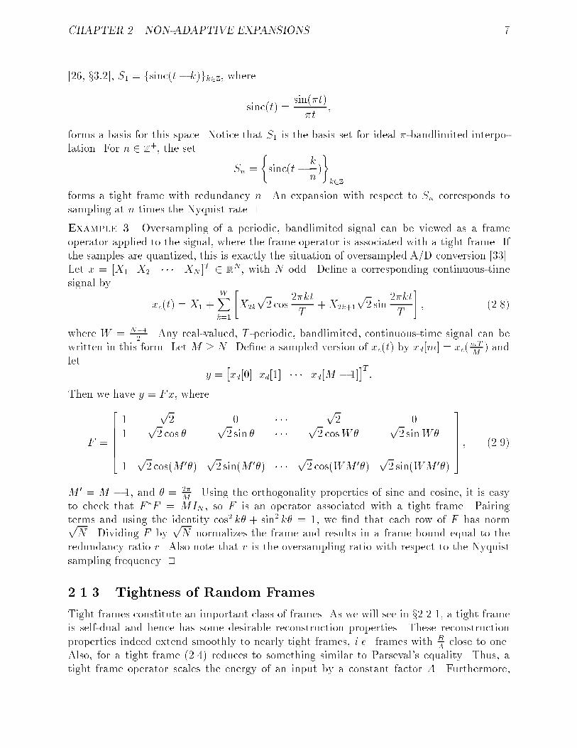
Example 3. Oversampling of a periodic, bandlimited signal can be viewed as a frameoperator applied to the signal, where the frame operator is associated with a tight frame. Ifthe samples are quantized, this is exactly the situation of oversampled A/D conversion [33].Let x = [X1 X2 � � � XN ]T 2 R
N, with N odd. De�ne a corresponding continuous-timesignal by
xc(t) = X1 +WXk=1
"X2k
p2 cos
2�kt
T+X2k+1
p2 sin
2�kt
T
#; (2.8)
where W = N�12 . Any real-valued, T -periodic, bandlimited, continuous-time signal can be
written in this form. Let M � N . De�ne a sampled version of xc(t) by xd[m] = xc(mTM) and
lety = [xd[0] xd[1] � � � xd[M � 1]]
T:
Then we have y = Fx, where
F =
26666641
p2 0 � � � p
2 0
1p2 cos �
p2 sin � � � � p
2 cosW�p2 sinW�
......
......
...
1p2 cos(M 0�)
p2 sin(M 0�) � � � p
2 cos(WM 0�)p2 sin(WM 0�)
3777775 ; (2.9)
M 0 = M � 1, and � = 2�M. Using the orthogonality properties of sine and cosine, it is easy
to check that F �F = MIN , so F is an operator associated with a tight frame. Pairingterms and using the identity cos2 k� + sin2 k� = 1, we �nd that each row of F has normpN . Dividing F by
pN normalizes the frame and results in a frame bound equal to the
redundancy ratio r. Also note that r is the oversampling ratio with respect to the Nyquistsampling frequency. �
2.1.3 Tightness of Random Frames
Tight frames constitute an important class of frames. As we will see in x2.2.1, a tight frameis self-dual and hence has some desirable reconstruction properties. These reconstructionproperties indeed extend smoothly to nearly tight frames, i.e. frames with B
Aclose to one.
Also, for a tight frame (2.4) reduces to something similar to Parseval's equality. Thus, atight frame operator scales the energy of an input by a constant factor A. Furthermore,

CHAPTER 2. NON-ADAPTIVE EXPANSIONS 8
it is shown in x2.2.4 that some properties of \typical" frame operators depend only on theredundancy. This motivates our interest in the following theorem.
Theorem 2.2: Tightness of Random FramesLet f�Mg1M=N be a sequence of frames in RN such that �M is generated by choosing Mvectors independently with a uniform distribution on the unit sphere in RN. Let FM be theframe operator associated with �M . Then, in the mean squared sense,
1
MFM
�FM �! 1
NIN elementwise as M �! 1:
Proof: See xA.3. �Theorem 2.2 shows that a sequence of random frames with increasing redundancy will
approach a tight frame. Note that although the proof in Appendix A uses an unrelatedstrategy, the constant 1=N is intuitive: If �M is a tight frame with normalized elements,then we have FM
�FM = MNIN because the frame bound equals the redundancy of the frame.
Numerical experiments were performed to con�rm this behavior and observe the rateof convergence. Sequences of frames were generated by successively adding random vectors(chosen according to the appropriate distribution) to existing frames. Results shown inFigures 2.1 and 2.2 are averaged results for 200 sequences of frames in R4. Figure 2.1 showsthat A
Mand B
Mconverge to 1
N. Figure 2.2 shows that B
Aconverges to one.
In Theorem 2.2, the uniformity of the frame elements over the unit sphere is a necessarycondition. This is illustrated by the following example.
Example 4. Suppose sequences of frames in R2 is generated by choosing vectors 'k =
[cos � sin �]T , where � is uniformly distributed on [0; �2 ]. Then
1
MFM
�FM !"
12
12�
12�
12
#elementwise asM !1:
Thus the sequence of frames does not approach a tight frame. We can make a few additionalobservations. The eigenvalues of "
12
12�
12�
12
#are �1 =
12(1 +
1�) and �2 =
12(1 � 1
�), with corresponding eigenvectors f1 =
1p2[1 1]T and
f2 =1p2[1 � 1]T , respectively. The eigenvectors f1 and f2 are the vectors that maximize
and minimize, respectively,
E
"MXk=1
jhf; 'kij2#
over all unit-norm f . This example reinforces the notion that tightness of frames correspondsto directional uniformity. �
2.2 Reconstruction from Frame Coe�cients
At this point, the usage of frames in signal analysis is not yet justi�ed because we have notconsidered the problem of reconstructing from frame coe�cients.

CHAPTER 2. NON-ADAPTIVE EXPANSIONS 9
2 4 6 8 10 12 140.05
0.1
0.15
0.2
0.25
0.3
0.35
0.4
0.45
0.5
log2(M)
Nor
mal
ized
fram
e bo
unds
B/M
A/M
Figure 2.1: Normalized frame bounds for random frames in R4.
2 4 6 8 10 12 141
2
3
4
5
6
7
8
9
log2(M)
Rat
io o
f fra
me
boun
ds B
/A
Figure 2.2: Ratios of frame bounds for random frames in R4.

CHAPTER 2. NON-ADAPTIVE EXPANSIONS 10
In x2.2.1, we review the basic properties of reconstructing from (unquantized) frame coef-�cients. This material is adapted from [6]. The subsequent sections consider the problem ofreconstructing an estimate of an original signal from quantized frame coe�cients. Classicalmethods are limited by the assumption that the quantization noise is white. Our approachuses deterministic qualities of quantization to arrive at the concept of consistent reconstruc-tion. Consistent reconstruction methods yield smaller reconstruction errors than classicalmethods.
2.2.1 Unquantized Case
Let � be a frame, assuming the notation of x2.1.1. In this subsection, we consider theproblem of recovering f from fhf; 'kigk2K.
Recall that F �F is invertible. We can say furthermore that
B�1IN � (F �F )�1 � A�1IN : (2.10)
Definition. The dual frame of � is e� = ff'kgk2K, wheref'k = (F �F )�1'k; 8 k 2 K: (2.11)
For a tight frame, (2.11) simpli�es to
f'k = A�1'k; 8 k 2 K: (2.12)
Proposition 2.3. e� is a frame with frame bounds B�1 and A�1, i.e.
B�1kfk2 � Xk2K
jhf; f'kij2 � A�1kfk2:
The associated frame operator eF : H ! CM satis�es eF = F (F �F )�1, eF � eF = (F �F )�1, andeF �F = IN = F � eF . Also, eFF � = F eF � is the orthogonal projection operator, in CM , onto
Ran(F ) = Ran( eF ).Proof: See [6, p. 59]. �
A consequence of eF � eF = (F �F )�1 is that the dual of e� is �. Another of the conclusionsof Proposition 2.3 gives us the desired reconstruction formula: Namely, eF �F = IN implies
f = eF �Ff =Xk2K
hf; 'kif'k: (2.13)
This formula is reminiscent of (2.2). The di�erence is that in (2.2), one set of vectors playsthe roles of both � and e�. This is because the set in (2.3) is a tight frame in CN . In analogyto (2.13), since F � eF = IN , we can also write
f = F � eFf =Xk2K
hf; f'ki'k: (2.14)
Comparing (2.13) and (2.14) emphasizes the \dual" nature of � and e�.

CHAPTER 2. NON-ADAPTIVE EXPANSIONS 11
The derivation of (2.14) obscures the fact that, when M > N , there should be manyways to write f as a linear combination of vectors from �. After all, there is an N -elementsubset of � that spans H. What is special about the expansion in (2.14)? This question ispartially answered by the following proposition.
Proposition 2.4. If f =P
k2K ck'k for some set of coe�cients fckgk2K, thenXk2K
jckj2 �Xk2K
jhf; f'kij2 ; (2.15)
with equality only if ck = hf; f'ki for all k 2 K.Proof: See [6, p. 61]. �
The norm-minimizing property of (2.15) holds in the \dual" sense also: If
f =Xk2K
hf; 'kiuk;
then Xk2K
jhuk; gij2 �Xk2K
jhf'k; gij2for all g 2 H. Also, using (2.13) has advantages over other possible reconstruction formulaswhen the frame coe�cients are not known exactly (see x2.2.2).
Sometimes we can reconstruct, or approximately reconstruct, without explicitly �ndingthe dual frame through (2.11). For example, if � is a tight frame, by substituting (2.12)into (2.13), we can write f = A�1P
k2Khf; 'ki'k. It is interesting to see how this extendssmoothly to the case that � is close to tight, i.e. A is close to B.
Let � = BA� 1. If 0 < �� 1, F �F � A+B
2 IN , so (F �F )�1 � 2A+B IN . Precisely,
f =2
A+B
Xk2K
hf; 'ki'k +Rf; (2.16)
where R = IN � 2A+B
F �F . (This is valid for any �.) Let
f0 =2
A+B
Xk2K
hf; 'ki'k: (2.17)
It can be shown that kRk � B�AB+A = �
2+� ; therefore kf � f0k � �2+�kfk, so (2.17) gives an
estimate for f with bounded error. The iteration
fn = fn�1 +2
A+B
Xk2K
[hf; 'ki � hfn�1; 'ki]'k
gives a sequence of estimates satisfying
kf � fnk �
�
2 + �
!n+1kfk: (2.18)
The dependence on � in (2.18) shows that for a �xed error tolerance, less computation isrequired for reconstruction in a tight or nearly tight frame.
CHAPTER 2. NON-ADAPTIVE EXPANSIONS 12
2.2.2 Classical Method
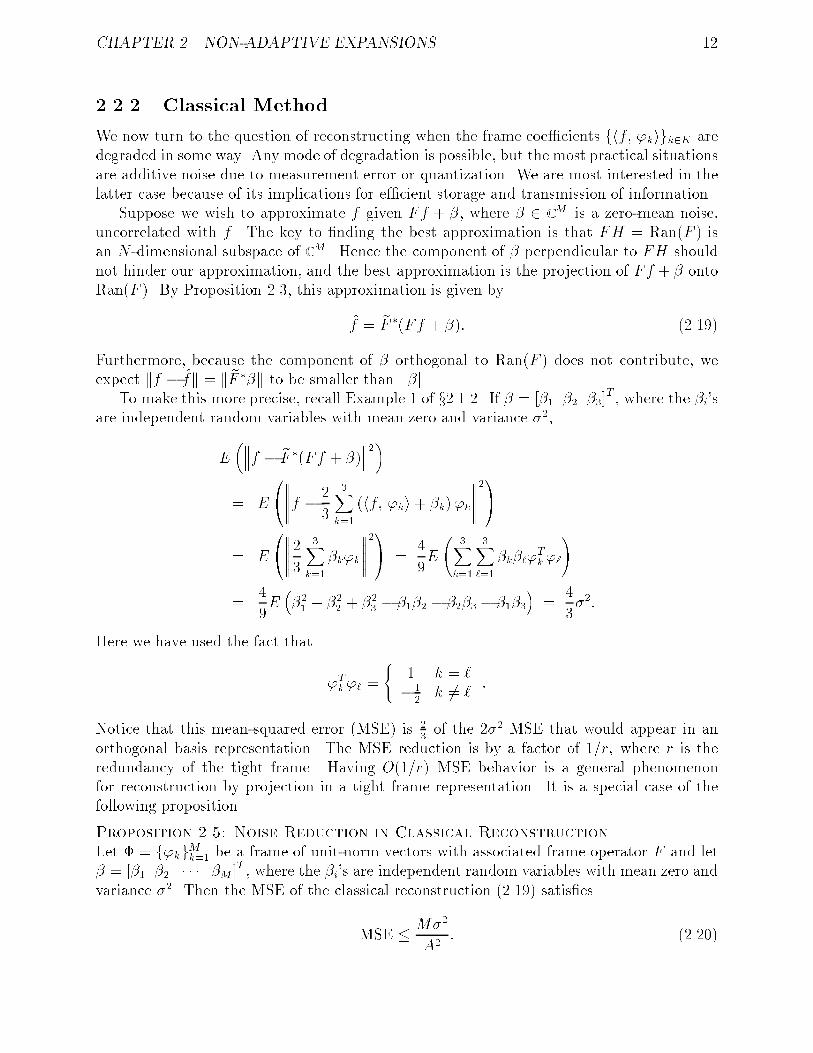
We now turn to the question of reconstructing when the frame coe�cients fhf; 'kigk2K aredegraded in some way. Any mode of degradation is possible, but the most practical situationsare additive noise due to measurement error or quantization. We are most interested in thelatter case because of its implications for e�cient storage and transmission of information.
Suppose we wish to approximate f given Ff + �, where � 2 CM is a zero-mean noise,
uncorrelated with f . The key to �nding the best approximation is that FH = Ran(F ) isan N -dimensional subspace of CM . Hence the component of � perpendicular to FH shouldnot hinder our approximation, and the best approximation is the projection of Ff + � ontoRan(F ). By Proposition 2.3, this approximation is given by
f = eF �(Ff + �): (2.19)
Furthermore, because the component of � orthogonal to Ran(F ) does not contribute, weexpect kf � fk = k eF ��k to be smaller than k�k.
To make this more precise, recall Example 1 of x2.1.2. If � = [�1 �2 �3]T , where the �i's
are independent random variables with mean zero and variance �2,
E� f � eF �(Ff + �)
2�
= E
0@ f � 2
3
3Xk=1
(hf; 'ki + �k)'k
21A
= E
0@ 233X
k=1
�k'k
21A =
4
9E
3X
k=1
3X`=1
�k�`'Tk '`
!
=4
9E��21 + �22 + �23 � �1�2 � �2�3 � �1�3
�=
4
3�2:
Here we have used the fact that
'Tk'` =
(1 k = `�1
2k 6= `
:
Notice that this mean-squared error (MSE) is 23of the 2�2 MSE that would appear in an
orthogonal basis representation. The MSE reduction is by a factor of 1=r, where r is theredundancy of the tight frame. Having O(1=r) MSE behavior is a general phenomenonfor reconstruction by projection in a tight frame representation. It is a special case of thefollowing proposition.
Proposition 2.5: Noise Reduction in Classical ReconstructionLet � = f'kgMk=1 be a frame of unit-norm vectors with associated frame operator F and let� = [�1 �2 � � � �M ]
T , where the �i's are independent random variables with mean zero andvariance �2. Then the MSE of the classical reconstruction (2.19) satis�es
MSE � M�2
A2: (2.20)

CHAPTER 2. NON-ADAPTIVE EXPANSIONS 13
Furthermore, if the frame is tight, (2.20) holds with equality, giving
MSE =N2�2
M=N�2
r: (2.21)
Proof: See xA.4. �Now consider the case where the degradation is due to quantization. Let x 2 R
N andy = Fx, where F 2 RM�N is a frame operator. Suppose y = Q(y), where Q : RM ! R
M isa scalar quantization function, i.e. Q(y) = [q(y1) q(y2) : : : q(yM)]T , where q : R! R is ascalar quantization function.
One approach to approximating x given y is to treat the quantization noise y� y as ran-dom, independent in each dimension, and uncorrelated with y. These assumptions make theproblem tractable using statistical techniques. The problem reduces to the previous prob-lem, and x = eF �y is the best approximation. Strictly speaking, however, the assumptionson which this reconstruction is based are not valid because y� y is a deterministic quantitydepending on y, with interplay between the components.
2.2.3 Consistent Reconstruction
The shortcoming of the classical reconstruction method is that it disregards deterministicproperties of quantization. As a result, the reconstruction may have a di�erent quantizedvalue than the original. Using the term introduced by Thao and Vetterli [33], we say thatthe reconstruction may be inconsistent.
Definition. We say that x is a consistent estimate of x or a consistent reconstruction ifQ(F x) = Q(Fx). A reconstruction that is not consistent is said to be inconsistent.
In words, we would say that an estimate is consistent if it is the same as its quantizedversion. Another way to understand consistency is in terms of partitions. Q induces apartitioning of RM. (We can temporarily remove the restriction that Q is a scalar quantizerand require only that the partition regions are convex.) This quantization also induces apartitioning of RN through the inverse image of Q�F . The partition of RN can be viewed inanother way: Since Q partitions RM, it also partitions the N -dimensional subspace F (RN).Mapping back to RN using eF � gives the partition of RN induced by Q. A consistent estimateis simply one that falls in the same partition region as the original.
All of these concepts are illustrated for N = 2 and M = 3 in Figure 2.3. The ambi-ent space is RM. The cube represents the partition region in RM containing y = Fx andhas codebook value y. The plane is F (RN) and hence is the subspace within which anyunquantized value must lie. The intersection of the plane with the cube gives the shadedtriangle within which a consistent estimate must lie. Projecting to F (RN), as in the classicalreconstruction method, removes the out-of-subspace component of y� y. As illustrated, thistype of reconstruction is not necessarily consistent. For further geometric interpretation ofquantized frame expansions, refer to Appendix B.
With no assumptions on Q other than that the partition regions be convex, a consistentestimate can be determined using the projection onto convex sets (POCS) algorithm. In this

CHAPTER 2. NON-ADAPTIVE EXPANSIONS 14
in-subspace error
y
Fx
out-of-sub-space error
ℜM
F ℜN( )
Figure 2.3: Illustration of consistent reconstruction
case that implies generating a sequence of estimates by alternately projecting on F (RN) andQ�1(y).
When Q is a scalar quantizer, a linear program can be used to �nd consistent estimates.For i = 1, 2, : : :, M , denote the quantization stepsize in the ith component by �i. Fornotational convenience, assume that the reproduction values lie halfway between decisionlevels. Then for each i, jyi � yij � �i
2 . To obtain a consistent estimate, for each i we musthave
j(F x)i � yij � �i
2:
Expanding the absolute value, we �nd the constraints
F x � 1
2� + y and F x � �1
2� + y
where � = [�1 �2 : : : �M ]T , and the inequalities are elementwise. These inequalities can

CHAPTER 2. NON-ADAPTIVE EXPANSIONS 15
be combined into "F�F
#x �
"12�+ y
12�� y
#: (2.22)
The formulation (2.22) shows that x can be determined through linear programming [31].The feasible set of the linear program is exactly the set of consistent estimates, so an arbitrarycost function can be used.
A linear program always returns a corner of the feasible set [31, x8:1], so this type ofreconstruction will not be close to the centroid of the partition cell. Since the cells areconvex, one could use several cost functions to (presumably) get di�erent corners of thefeasible set and average the results. Another approach is to use a quadratic cost functionequal to the distance from the projection estimate given by (2.19). Both of these methodswill reduce the MSE by a constant factor. They do not change the asymptotic behavior ofthe MSE as the redundancy r is increased.
2.2.4 Error Bounds
In this subsection, we concern ourselves with bounds on the MSE in estimating x from y.Our fundamental premise is that any reconstruction method that gives consistent estimatesis asymptotically (in the redundancy r) optimal. We now prove two bounds that supportthis conviction: �rst, an O(1=r2) MSE lower bound for any reconstruction algorithm; andsecond, an O(1=r2) MSE upper bound for consistent reconstruction. Since we are varying r,we must consider sequences of frames with growing redundancy.
Theorem 2.6: MSE Lower BoundFor any set of quantized frame expansions, any reconstruction algorithm will yield an MSEthat can be lower bounded by an O(1=r2) expression.3
Proof: The proof of this general result is given under the guise of a more restricted resultin [35]. There it is proven that when the frame operators correspond to oversampled A/Dconversion (see x2.1.2), any reconstruction algorithm will yield an MSE that can be lowerbounded by an O(1=r2) expression. The proof is based on counting the number of cells inthe partition of RN and using Zador's formula. The only frame-speci�c property that is usedcorresponds to requiring that elements of the frame not be parallel. Having parallel frameelements would reduce the number of cells in the partition and hence increase the MSE.Therefore the proof extends to the general case. �
Proposition 2.7: MSE Upper Bound (Restricted Case)Let x be such that it has a probability density.4 Consider quantized frame expansions ofx with frame corresponding to the frame operator (2.9) and quantization stepsize �. Forsu�ciently small (�xed) �, a consistent reconstruction algorithm will yield an MSE that canbe upper bounded by an O(1=r2) expression.Proof: The proof is based on a correspondence between vectors in RN and periodic, ban-dlimited, continuous-time signals. Let xc(t) be de�ned as in (2.8), where T is arbitrary. Then
3Actually, we must exclude the case where x has a degenerate distribution that allows for perfect recon-struction. This point is not emphasized in [35].
4This is to eliminate degenerate distributions for x.

CHAPTER 2. NON-ADAPTIVE EXPANSIONS 16
quantized frame expansion of x is equivalent to oversampled A/D conversion of xc(t). Ac-cording to Thao and Vetterli [33, Thm. 4.1], the MSE can be upper bounded by an O(1=r2)expression. One requirement in applying their result is that xc(t) must have su�cient quan-tization threshold crossings. In our more general framework, this corresponds to requiringthat the distribution of x not be overly concentrated inside a sphere of radius �.5 Since xhas a probability density, this can be assured by choosing � su�ciently small. �
Conjecture 2.8: MSE Upper BoundUnder very general conditions, for any set of quantized frame expansions, any algorithmthat gives consistent estimates will yield an MSE that can be upper bounded by an O(1=r2)expression.
For this general upper bound to hold, some sort of non-degeneracy condition is requiredbecause we can easily construct a sequence of frames with increasing r for which the framecoe�cients give no additional information as r is increased. For example, we can start withan orthonormal basis and increase r by adding copies of vectors already in the frame. Puttingaside pathological cases, simulations for quantization of a source uniformly distributed on[�1; 1]N support this conjecture. Simulations were performed with three types of framesequences:
I. A sequence of frames corresponding to oversampled A/D conversion, as given by(2.9). This is the case in which we have a provable O(1=r2) MSE upper bound.
II. For N = 3, 4, and 5, Hardin, Sloane and Smith have numerically found arrange-ments of up to 130 points on N -dimensional unit spheres that maximize theminimum Euclidean norm separation [16].
III. Frames generated by randomly choosing points on the unit sphere according toa uniform distribution.
Simulation results are given in Figure 2.4. The dashed, dotted, and solid curves correspondto frame types I, II, and III, respectively. The data points marked with +'s correspondto using a linear program based on (2.22) to �nd consistent estimates. The data pointsmarked with �'s correspond to classical reconstruction. The important characteristics ofthe graph are the slopes of the curves. Note that O(1=r) MSE corresponds to a slope of-3.01 dB/octave and O(1=r2) MSE corresponds to a slope of -6.02 dB/octave. The consistentreconstruction algorithm exhibits O(1=r2) MSE for each of the types of frames. The classicalmethod exhibits O(1=r) MSE behavior, as expected. It is particularly interesting to notethat the performance with random frames is as good as with either of the other two typesof frames.
Note that in light of Theorem 2.2, it may be useful to try to prove Conjecture 2.8 onlyfor tight frames.
5In most cases, we assume quantizer o�sets such that zero is either a reconstruction value or a boundaryvalue. By randomizing the quantizer o�set, we can remove this condition.

CHAPTER 2. NON-ADAPTIVE EXPANSIONS 17
3 3.5 4 4.5 5 5.5−72
−70
−68
−66
−64
−62
−60
−58
−56
−54
log2(r)
MS
E (
dB)
Classical reconstruction
Consistent reconstruction
Frame Type���� I� � � � � � �� II������� III
Figure 2.4: Experimental results for reconstruction from quantized frame expansions. ShowsO(1=r2) MSE for consistent reconstruction and O(1=r) MSE for classical reconstruction.
2.2.5 Rate-Distortion Tradeo�s
Our discussion of quantized frame expansions has focused on expected distortion withoutconcern for rate. In this subsection we begin consideration of rate-distortion tradeo�s.
We have demonstrated that optimal reconstruction techniques give an MSE proportionalto 1=r2. It is well known that in orthogonal representations the MSE is proportional to�2. This extends to the frame case as well. Thus we have two ways to reduce the MSE byapproximately a factor of four:
� double r;
� halve �.
A priori, there is no reason to think that these options each have the same e�ect on therate. As the simplest possible case, suppose a frame expansion is stored (or transmitted)as M B-bit numbers, for a total rate of MB bits per sample. Doubling r gives 2M B-bitnumbers, for a total rate of 2MB bits per sample. On the other hand, halving � results inM (B + 1)-bit numbers for a rate of only M(B + 1) bits per sample.
This argument suggests that halving � is always the better option, but a few commentsare in order. One caveat is that in some situations, doubling r and halving � may havevery di�erent costs. For example, in oversampled A/D conversion, the monetary cost ofhalving � is much higher than that of doubling r because it requires precision trimmedanalog electronics. This is a major motivating factor for oversampling.

CHAPTER 2. NON-ADAPTIVE EXPANSIONS 18
Also, if r is doubled, storing the result as 2M B-bit values is far from the best thing todo. This is because many of the M additional numbers give little or no information on x.A conclusion of Zamir and Feder [38] was described by Zamir as, \one good measurementis better than many noisy ones" [39]. It is important to note that although they considerquantization noise, they do not consider consistency. These topics are discussed further inAppendix B; Appendix C explores the use of quantized frame expansion as the �rst stage ina lattice quantizer.
We conclude this chapter by noting that it is complicated to get e�cient signal rep-resentations from highly redundant quantized frame expansions. Because of redundancy,each frame coe�cient does not give the same amount of information on x; one way to getan e�cient representation would be to retain only the frame coe�cients that give a lot ofinformation on x. This is essentially the theme of the next chapter.

Chapter 3
Adaptive Expansions
In this chapter, we broaden our approach to �nding linear expansions by allowing the basisfunctions of the expansion to vary depending on the signal. However, we are not adapting inthe traditional sense of making �ne adjustments depending on an error signal. Instead, ourbasic tool is the matching pursuit algorithm of [20] in which the adaptation is in the choiceof basis functions from a �xed dictionary (frame).
In x3.1, we introduce the optimal approximation problem in order to establish its com-putational intractability. The matching pursuit algorithm, described in x3.2, is a greedyalgorithm for �nding approximate solutions to the approximation problem. Quantization ofcoe�cients in matching pursuit leads to many interesting issues; some of these are discussedin x3.3. Along with exploring general properties of matching pursuit, we are interested in itsapplication to compressing data vectors in RN. A general vector compression method basedon matching pursuit is described in x3.4.
3.1 The Optimal Approximation Problem
At the end of the previous chapter, we noted that the set of coe�cients from a highlyredundant frame expansion are, without sophisticated coding, an ine�cient representationof a signal. We expect to �nd more e�cient representations by forming a linear expansionwith respect to a subset of the original frame. This problem is formalized below.
Definition [7, Ch. 2]. Let a dictionary D be a frame in H. Let � > 0 and L 2 Z+. For
f 2 H, an expansion
~f =LXi=1
�i'ki ; (3.1)
where �i 2 C and 'ki 2 D, is called an (�; L)-approximation if k ~f � fk < �. An expansion(3.1) that minimizes k ~f � fk is called an L-optimal approximation.
Since the �i's are not subject to quantization, these approximation problems do notexactly correspond to �nding rate-distortion optimal representations for �xed L. Also, thisformulation does not account for the fact that, with entropy coding, the rate associated withf'kigLi=1 may depend on the choice of dictionary elements. Nevertheless, we are discouraged
19

CHAPTER 3. ADAPTIVE EXPANSIONS 20
from attempting to �nd optimal quantized representations by the following theorem.
Theorem 3.1: Intractability of Optimal Approximation [7]Let k � 1 and let D be a dictionary that contains O(Nk) vectors. Let 0 < 1 < 2 < 1 andlet L 2 Z+ such that 1N � L � 2N . For any given � > 0 and f 2 H, determining whetheran (�; L)-approximation exists is NP-complete. Finding the L-optimal approximation isNP-hard.Proof: See [7, Ch. 2]. �
3.2 Matching Pursuit
The intractability of L-optimal approximation stems from the number of ways to choose Ldictionary elements. The complexity is reduced if the dictionary elements are chosen one at atime instead of L at once. This reduction of a \global" problem to simpler \local" problemsis the de�ning characteristic of a greedy algorithm. Matching pursuit is a greedy algorithmfor �nding approximate solutions to the L-optimal approximation problem. It progressivelyre�nes a signal estimate instead of �nding L components jointly.
Matching pursuit was introduced to the signal processing community in the context oftime-frequency analysis by Mallat and Zhang [20]. Mallat and his students have uncoveredmany of its properties [7, 8, 9, 40].
3.2.1 Algorithm
Let D = f'kgMk=1 � H be a frame. We impose the additional constraint that k'kk = 1for all k. We will call D our dictionary of vectors. Matching pursuit is an algorithm torepresent f 2 H by a linear combination of elements of D. Furthermore, matching pursuitis an iterative scheme that at each step attempts to approximate f as closely as possible in agreedy manner. We expect that after a few iterations we will have an e�cient approximaterepresentation of f .
In the �rst step of the algorithm, k0 is selected such that jh'k0 ; fij is maximized. Thenf can be written as its projection onto 'k0 and a residue R1f ,
f = h'k0 ; fi'k0 +R1f:
The algorithm is iterated by treating R1f as the vector to be best approximated by a multipleof 'k1. At step p + 1, kp is chosen to maximize jh'kp ; Rpfij and
Rp+1f = Rpf � h'kp ; Rpfi'kp : (3.2)
Identifying R0f = f , we can write
f =n�1Xi=0
h'ki ; Rifi'ki +Rnf: (3.3)
Hereafter we will denote h'ki ; Rifi by �i.

CHAPTER 3. ADAPTIVE EXPANSIONS 21
3.2.2 Discussion
Matching pursuit is similar to a class of algorithms used in statistics called projection pursuits.The proof of the convergence of projection pursuits given in [18] can be used to provethe convergence of matching pursuit in in�nite dimensional spaces. In in�nite dimensionalspaces, the convergence can be quite slow. However, the convergence is exponential in �nitedimensional spaces [7, x3:1].
Since �i is determined by projection, �i'ki ? Ri+1f . Thus we have the \energy conser-vation" equation
kRifk2 = kRi+1fk2 + �2i : (3.4)
This fact, the selection criterion for ki, and the fact that D spans H, can be combined fora simple convergence proof for �nite dimensional spaces. In particular, the energy in theresidue is strictly decreasing until f is exactly represented.
In the language of x3.1, matching pursuit can be viewed as �nding a 1-optimal approx-imation and then iteratively �nding 1-optimal approximations on the resulting residues. IfD is an orthonormal basis, matching pursuit �nds the optimal expansion. For an arbitrarydictionary, however, matching pursuit does not generally �nd optimal expansions. In fact, ifno two elements of the dictionary are orthogonal, matching pursuit expansions are not onlynot optimal, but they do not converge in a �nite number of steps except on a set of measurezero [7, x3:1].
In the following, detailed operation counts and other measures of complexity will not begiven since the emphasis is not on implementation details. One point to note is that the fullset of inner products fh'i; RpfigMi=1 need not be computed at each iteration. By (3.2),
h'i; Rp+1i = h'i; Rpi � h'kp ; Rpih'i; 'kpi: (3.5)
In (3.5), h'i; Rpi and h'kp ; Rpi are known from the previous iteration, so only h'i; 'kpimust be computed. Depending on the dictionary structure, this may involve a table lookupor a simple calculation. Alternatively, the dictionary can be structured so that only a fewsuch inner products are nonzero.
Note that the output of a matching pursuit expansion is not only the coe�cients (�0, �1,: : : ), but also the indices (k0, k1, : : : ). For storage and transmission purposes, we will haveto account for the indices.
3.2.3 Orthogonalized Matching Pursuits
It was noted that, even in a �nite dimensional space, matching pursuit is not guaranteed toconverge in a �nite number of iterations. This is a serious drawback when exact (or veryprecise) signal expansions are desired, especially since an optimal algorithm would choose abasis from the dictionary and get an exact expansion in N steps. The cause of this drawbackis that at step p+ 1, 'kp is not necessarily chosen orthogonal to Span(f'kigp�1i=0 ).
The matching pursuit algorithm can be modi�ed to insure that at each iteration thecontribution to the linear expansion is orthogonal to all previous terms. Convergence in Nsteps is then guaranteed. A simple method of accelerating convergence through orthogonal-ization is described below [28]. The selection of dictionary elements is the same as before.

CHAPTER 3. ADAPTIVE EXPANSIONS 22
After a dictionary element 'kp is chosen, it is orthogonalized with respect to f'kigp�1i=0 beforethe residue Rpf is calculated. (Because of the orthogonalization, no dictionary element ischosen twice.) This insures that Rp+1f is orthogonal to 'ki for i = 0; 1; : : : ; p. A betterorthogonalization method is presented by Kalker and Vetterli in [19].
It has been noted by several authors [7, 19, 36] that for a small number of iterations, or-thogonal matching pursuit does not converge signi�cantly faster than the non-orthogonalizedversion. For this reason, orthogonal matching pursuit is not considered hereafter.
3.2.4 Relationship to the Karhunen-Lo�eve Transformation
In this section, we forge an analogy between matching pursuit and the Karhunen-Lo�evetransform (KLT). Our aim is to show that matching pursuit has some of the propertiesthat make the KLT useful in transform coding. We assert that matching pursuit acts as auniversal transform for transform coding.
For a stationary, vector-valued random process X, the Karhunen-Lo�eve transform is theunique orthogonal transform U such that Y = UX has a diagonal covariance matrix with theeigenvalues appearing in descending order on the diagonal [21, x1:2:4]. Note that determiningthe KLT requires knowledge of the distribution of X. Approximating the KLT from data isessentially the same as principal component analysis [17].
It is well known that the KLT is the optimal transform for transform coding. Since thelimitations to this result are not as well known, we state the following theorem paraphrasedfrom [13]:
Theorem 3.2: Optimality of the Karhunen-Lo�eve TransformConsider the transform coding of a jointly Gaussian random process. Suppose the quanti-zation is �ne enough to use high resolution approximations, and that arbitrary real (non-integer) values can be allocated to the resolution of each (scalar) quantizer. Then the KLTachieves the lowest overall distortion of any orthogonal transform.Proof: See [13, x8:6]. �
Two properties of the KLT that make it good for transform coding are qualitativelymimicked by matching pursuit:
1. Energy compaction: For 1 � i � N � 1, the energy in fy1; y2; : : : ; yig ismaximum over all orthogonal transforms. For this reason the KLT is said to giveoptimal energy compaction.
2. Principal axes: If X has an ellipsoidal distribution (as when X is Gaussian), theith transformed variable yi corresponds to the ith principal axis of the ellipsoid.This is closely coupled with energy compaction, since the ith principal axis is thedirection in which there is the ith largest energy.
We �rst explore the energy compaction properties of matching pursuit. The criterionfor the choice of ki makes some degree of energy compaction obvious. Since we only solve1-optimal approximation problems, matching pursuit does not always give optimal energycompaction when more than one iteration is performed. However, in matching pursuit we areoptimizing on a sample-by-sample basis, as opposed to looking at average performance with

CHAPTER 3. ADAPTIVE EXPANSIONS 23
100
101
102
0.93
0.94
0.95
0.96
0.97
0.98
0.99
1
Redundancy r
Fra
ctio
n of
ene
rgy
in fi
rst c
oeffi
cien
t
uncorrelated source
correlated source
Figure 3.1: Energy compaction achieved using matching pursuit on an R2-valued source.
a �xed transform. Therefore matching pursuit generally gives much more energy compactionthan the KLT. In particular, matching pursuit will give energy compaction even if X has adiagonal covariance matrix, in which case the KLT gives no energy compaction.
Energy compaction performance was assessed by simulation. In R2, two sources wereused:
� An uncorrelated zero-mean Gaussian source X � N (0; I).
� A Gaussian source
X � N 0; AT
�
"1 00 0:2
#A�
!(3.6)
where A� is a Givens plane rotation matrix (� = �3 ).
Dictionaries of the form
D =
8<:"cos
2�k
Msin
2�k
M
#T9=;M�1
k=0
(3.7)
were used. The results are shown in Figure 3.1. Using matching pursuit, more than 93%of the energy is captured in the �rst coe�cient, and the energy compaction increases withincreasing dictionary redundancy. The KLT would give 1
2and 5
6of the energy in the �rst
coe�cient for the uncorrelated and correlated sources, respectively.Simulations were also performed for R4-valued sources. Two sources were used:

CHAPTER 3. ADAPTIVE EXPANSIONS 24
100
101
0.5
0.6
0.7
0.8
0.9
1
Redundancy r
Fra
ctio
n of
ene
rgy
in fi
rst c
oeffi
cien
t
uncorrelated source
correlated source
Figure 3.2: Energy compaction achieved using matching pursuit on an R4-valued source.
� An uncorrelated zero-mean Gaussian source X � N (0; I).
� A correlated zero-mean Gaussian source formed by placing a �rst-order autoregressivesource with correlation 0.9 in blocks of length 4.
Dictionaries were generated from maximally spaced points on the unit sphere [16]. Theresults are given in Figure 3.2. As expected, the energy compaction in the �rst componentincreases with r, ranging from about 0:55 to 0:96. In this case, the KLT would give 1
4and
� 0:8817 of the energy in the �rst coe�cient for the uncorrelated and correlated sources,respectively. So in this experiment, matching pursuit always gives better energy compactionfor the uncorrelated source, and also does so for the highly correlated source when r > 8.
When X has an ellipsoidal distribution, geometric intuition suggests that 'k0 will morelikely be close to the principal axis than far from it. Similarly, given that 'k0 is nearlyparallel to the principal axis, the distribution of R0x will be ellipsoidal with principal axisequal to the second principal axis of the distribution of x. (Since the most we can possiblysay is that 'k0 usually is nearly parallel to the principal axis, this reasoning is somewhatweak.) We would like to formalize this intuition. In particular, we attempt to demonstratethat the indices ki can be used to estimate the principal axes and that the algorithm is likelyto choose indices that correspond to the KLT. We are however not asserting that it wouldbe ideal for the algorithm to choose indices corresponding to the KLT; matching pursuit isacting locally, while the KLT is based on global stationary statistics.
Methods for estimating the principal axes are not immediately obvious. We cannot simply

CHAPTER 3. ADAPTIVE EXPANSIONS 25
\average the 'k0's to estimate the �rst principal axis" because, with a su�ciently regularand dense dictionary and an ellipsoidal distribution, E'k0 = 0.
For example, consider quantization of the R2-valued source from (3.6), expanded usinga dictionary as in (3.7) with M = 199. Figure 3.3 shows histograms of k0 and k1 for 10000
samples. The peaks of the histograms are at fk0 = 33 and fk1 = 83. These correspond toangles (modulo �) of 66�
199and 166�
199, respectively. These are very close to angles of the principal
axes of the distribution, which are �3and 5�
6. Unfortunately, looking at peaks of histograms
is not very robust and is limited by the redundancy and regularity of the dictionary. Thus wewould like to use a method that involves averaging. As we noted, averaging 'k0's and 'k1'sis meaningless. Referring to Figure 3.3, this is because of the bimodality of the histograms.It also makes no sense to average the index numbers because this would not be invariant torenumberings of the dictionary, even those renumberings that maintain the natural order.1
Using a dictionary that is spread along half of the unit circle instead of the whole unit circlewould bias the estimates toward the center of the half-circle chosen. The proposed solutionis to use the histogram peaks as initial estimates of the principal axes and then \center" thedictionary around the corresponding vectors. For concreteness, suppose we are estimatingthe �rst principal axis. Suppose we have used matching pursuit to expand a set of samples.Let fk0 denote the histogram peak of the k0's. For themth sample, we increment the principalaxis estimate by '(k0)m if h'(k0)m; 'ek0i � 0, and by �'(k0)m otherwise. This procedure can beapplied in any dimension because it does not depend on an ordering of dictionary elements.A potential pitfall is that if the dictionary is not uniform, the histogram peak may be a poorinitial estimate.
Figure 3.4 shows simulation results for principal axis estimation using the methods dis-cussed above. The source is as given by (3.6) and the dictionary is as in (3.7) withM = 399.The error is measured as an angular error in radians. The �gure shows that both methods(looking only at histogram peaks and averaging using a peak as an initial estimate) giveincreasingly good estimates as data accumulates. The averaging method gives MSEs thatare lower by about a factor of ten.
Simulations were also conducted with the same R4-valued autoregressive source as before.A dictionary of 130 maximally spaced unit vectors from [16] was used. The results are shownin Figure 3.5. The three pairs of curves correspond to estimating the �rst three principal axesof the distribution. The solid and dashed curves correspond to the averaging and histogrampeak methods, respectively. In this case the error is measured as Euclidean distance betweena unit vector in the true axis direction and the estimated axis direction. The results showthat while the �rst axis can be well-estimated, it is much harder to estimate the subsequentprincipal axes. The principal axes are probably easier to estimate when the eigenvalue spreadof the covariance of the source is large, but this is not explored further in this discussion.
Before moving on to study the e�ects of coe�cient quantization, we would like to explorethe dependence of index entropy on r. We have seen that increasing dictionary redundancyincreases energy compaction. The price to pay is that the entropy of the indices goes up.We explore this tradeo� through an example. This time we consider a non-ellipsoidal sourcegenerated by equally mixing sources of the form (3.6) with � equal to �
4 and ��4 . Figure 3.6
shows 1000 samples from this source. Note that the KLT for this source is simply the identity
1In higher dimensions, there would generally be no natural ordering to dictionary elements.

CHAPTER 3. ADAPTIVE EXPANSIONS 26
0 20 40 60 80 100 120 140 160 180 2000
50
100
150
200
250
300
Dictionary index
Cou
nt
Histogram of first index
0 20 40 60 80 100 120 140 160 180 2000
50
100
150
200
250
300
Dictionary index
Cou
nt
Histogram of second index
Figure 3.3: Histograms of indices chosen by matching pursuit
transformation. The samples were expanded using dictionaries of the form
D =
8<:"cos
�k
Msin
�k
M
#T9=;M�1
k=0
: (3.8)
Figure 3.7 shows the resulting energy compactions and index entropies as functions of r.(The index entropy should rightly be called a sample entropy. One must be very carefulto use large sample sizes to get relevant sample entropies.) We see that the entropy of the�rst index is proportional to log r, but the energy compaction levels o� rather quickly. So aslog r is increased, there are diminishing returns in energy compaction, but the cost increaseslinearly.
3.3 Quantized Matching Pursuit
Although matching pursuit has been applied to low bit rate compression problems [19, 23,24, 25, 36], which inherently require coarse coe�cient quantization, little work has been

CHAPTER 3. ADAPTIVE EXPANSIONS 27
101
102
103
104
10−5
10−4
10−3
10−2
10−1
histogram
averaging
Number of samples
MS
E o
f prin
cipl
e an
gle
estim
ate
Figure 3.4: Principal axis estimation using matching pursuit for an R2-valued source.
101
102
103
104
10−2
10−1
100
Axis 1
Axis 2
Axis 3
Number of samples
MS
E o
f nor
mal
ized
eig
enve
ctor
est
imat
e
Figure 3.5: Principal axes estimation using matching pursuit for an R4-valued source

CHAPTER 3. ADAPTIVE EXPANSIONS 28
−3 −2 −1 0 1 2 3−3
−2
−1
0
1
2
3
Figure 3.6: One thousand samples from a non-ellipsoidal source
100
101
102
0.6
0.65
0.7
0.75
0.8
0.85
0.9
0.95
1
Redundancy r
Fra
ctio
n of
ene
rgy
in fi
rst c
oeffi
cien
t
100
101
102
0
1
2
3
4
5
6
7
Redundancy r
Ent
ropy
of f
irst i
ndex
(bi
ts)
Figure 3.7: Energy compaction and index entropy as functions of redundancy r for a non-ellipsoidal source.
done to understand the qualitative e�ects of coe�cient quantization in matching pursuit. Inthis section we explore some of these e�ects. In x3.3.2, application of matching pursuit tocompress an R2-valued source is considered in great detail. The highlight of the subsectionis the generation of intricate partition diagrams. These partition diagrams demonstratethat matching pursuit expansions can be inconsistent. The issue of consistency in theseexpansions is explored in x3.3.3. The relationship between quantized matching pursuit andother vector quantization methods is discussed in x3.3.4.
3.3.1 Discussion
Coe�cients are quantized in any computer implementation of matching pursuit. When thequantization is �ne, it is generally safe to ignore this fact. For example, in all the simulationsof x3.2, coe�cient quantization does not make any qualitative di�erences. If the quantization

CHAPTER 3. ADAPTIVE EXPANSIONS 29
is coarse, as it must be for moderate to low bit rate compression applications, the e�ects ofquantization may be signi�cant.
De�ne quantized matching pursuit to be matching pursuit with non-negligible quantiza-tion of the coe�cients. We will denote the quantized coe�cients by c�i = Q[�i]. Note thatquantization destroys the orthogonality of the projection and residual, so the analog of (3.4)does not hold, i.e.
kRifk2 6= kRi+1fk2 + c�i2:Also, (3.5) does not hold.
We are assuming that the quantization of �i occurs before the residualRi+1f is calculated,and that the quantized version is used in determining the residual so that quantization errorsdo not propagate to subsequent iterations. Since c�i must be determined before �i+1, it isimplicit in this assumption is that the coe�cient quantization is scalar.
For any particular application, there are several design problems: a dictionary must bechosen, scalar quantizers must be designed, and the number of iterations (or a stoppingcriterion) must be set. In principle, these could be jointly optimized for a given sourcedistribution, distortion measure, and rate measure. In practice, this is an overly broadproblem. In the following subsection, we will make several choices, some of them arbitrary.
3.3.2 A Detailed Example
Consider quantization of a source with a uniform distribution on [�1; 1]2. Assume distortionis measured by squared Euclidean distance and rate is measured by codebook size. (Measur-ing rate by codebook size is natural when a �xed rate coder will be applied to the quantizeroutput, i.e. no entropy coding is used.) Also assume that two iterations will be performedwith a four element dictionary. Other constraints will be set as needed.
We �rst choose a dictionary. Guided by symmetry, we choose
D =
8<:"cos
(2k � 1)�
8sin
(2k � 1)�
8
#T9=;4
k=1
: (3.9)
A �rst impulse may be to use
D =
8<:"cos
(k � 1)�
4sin
(k � 1)�
4
#T9=;4
k=1
: (3.10)
In a detailed analysis, (3.9) was determined to lead to a better design. Also, (3.10) is notsymmetric with respect to the region of support of the distribution.
To begin with, assume that the quantization of coe�cients will be �ne. Then, since thedictionary is composed of pairs of orthogonal vectors, 'k0 ? 'k1. Thus once we have codedk0, k1 is determined for free. (As long as we are using a �ne quantization assumption, wewill actually force the k1 to be selected such that 'k0 ? 'k1.) It is easy to see that k0 willbe uniformly distributed on f1; 2; 3; 4g; thus, with or without entropy coding, k0 requires 2bits.

CHAPTER 3. ADAPTIVE EXPANSIONS 30
We now design the quantizers. The p.d.f. of �0 can be explicitly calculated as
p�0(y) =
8>><>>:2(p2 � 1)jyj jyj � 1
2
q2 +
p2
�2(jyj �q1 +
p2) 1
2
q2 +
p2 < jyj �
q1 +
p2
0 otherwise
: (3.11)
If the dictionary was not symmetric, (3.11) would have to be conditioned on k0. Since weare assuming �ne quantization, the best codebook constrained quantizer for �0 can be foundanalytically using a compandor model [13]. The optimal quantizer is
c�0 = G�1 �Qu �G(�0);
where
G(y) =
8>><>>:21=3
(2+p2)1=6
sgn(y) y4=3 jyj �p
2+p2
2
sgn(y)�q
1 + 1p2� 21=3
(2�p2)1=6�y sgn(y)�
q1 + 1p
2
�4=3�otherwise
;
and Qu is a uniform quantizer.Given �0, the distribution of �1 is uniform on [�j�0j; j�0j]. Since the quantization of c�0
is �ne, the distribution given c�0 is approximately the same. Thus the optimal quantizer for�1 is uniform.
We have yet to decide how to divide our bit rate between c�0 and c�1. Since 'k0 ? 'k1,the total distortion is simply the sum of the distortions created by each quantization. Wecan thus minimize distortion for a �xed rate by Lagrangian methods.
If we impose the constraint that the rate for c�1 must be constant, we get a codebook asin Figure 3.8(a). On the other hand, if we allow the rate for c�1 to be conditioned on c�0,we get a codebook as in Figure 3.8(b). (Actually, these codebooks are for the dictionary(3.10), but the observations and conclusions are still clear.) The two codebooks have 906and 900 elements, respectively, so they give approximately equal rates. The codebook inFigure 3.8(b) gives lower distortion, as is clear from the more uniform distribution of codevectors.
When the rate for c�1 depends on c�0, the Lagrangian optimization implies that the numberof quantization levels for �1 should be proportional to p b�0 . Using a codebook size of 304and choosing the proportionality constant appropriately yields the codebook and partitionshown in Figure 3.9. This codebook gives approximately 0:1561 bits worse performance thansimple uniform scalar quantization. (Recall that this includes two bits for k0.) Of course,this should not be too discouraging because the region of support and distribution of thesource in this simulation are tailor-made for uniform scalar quantization. As we will see inx3.4, matching pursuit tends to be e�ective when the number of iterations is less than thedimension of the space.
Figure 3.9 should be seen as a �rst approximation to the type of partition created bymatching pursuit because we forced 'k0 ? 'k1 . (This was part of the �ne quantizationassumption.) Let us now remove the �ne quantization assumption and allow the source tohave an arbitrary distribution on R2. Even with a known distribution, it is di�cult to �nd

CHAPTER 3. ADAPTIVE EXPANSIONS 31
−1 −0.5 0 0.5 1−1
−0.8
−0.6
−0.4
−0.2
0
0.2
0.4
0.6
0.8
1
−1 −0.5 0 0.5 1−1
−0.8
−0.6
−0.4
−0.2
0
0.2
0.4
0.6
0.8
1
(a) (b)
Figure 3.8: Codebook elements for quantization of a source with uniform distribution on[�1; 1]2. (a) Fixed rate for c�1. (b) Rate for c�1 conditioned on c�0.
−1 −0.5 0 0.5 1−1
−0.8
−0.6
−0.4
−0.2
0
0.2
0.4
0.6
0.8
1
Figure 3.9: Partitioning of [�1; 1]2 by matching pursuit with four element dictionary. A �nequantization assumption is used.

CHAPTER 3. ADAPTIVE EXPANSIONS 32
analytical expressions for optimal quantizers without using a �ne quantization assumption.Since we wish to use �xed, untrained quantizers, we will use uniform quantizers for �0 and�1. Since it will still generally be true that 'k0 ? 'k1 , it makes sense for the quantizationstepsizes for �0 and �1 to be equal.
The partitions generated by matching pursuit are very intricate. Figure 3.10 showsthe partitioning of the �rst quadrant when zero is a quantizer boundary value, i.e. thequantizer boundary points are fm�gm2Zand reconstruction points are f(m+ 1
2)�gm2Zfor
some quantization stepsize �. The yellow lines denote the partitions induced by selectionof k0. Then �0 is quantized, giving the cyan boundaries. Recall that the residue R1f is notnecessarily orthogonal to 'k0. Thus the selection of k1 introduces the magenta boundaries.Finally, the red boundaries come from quantizing �1. In Figure 3.10, most of the cells aresquares, but there are also some smaller cells. Unless the source distribution happens to havehigh density in the smaller cells, the smaller cells are ine�cient in a rate-distortion sense.The fraction of cells that are not square ! 0 as �! 0.
The partition is qualitatively di�erent when the quantizer boundary points aref(m+ 1
2)�gm2Zand reconstruction points are fm�gm2Z. The partition is shown in Fig-ure 3.11. The colors are the same as in Figure 3.10. The dotted magenta lines show bound-aries that are created by choice of k1 but are not important because c�1 = 0. (Similarly forthe dotted yellow line.) This partition also has mostly square cells. Compared to Figure 3.10,there are fewer of the \bad" small cells. As before, the fraction of non-square cells vanishesas �! 0.
The qualitative di�erence between Figure 3.9 and Figures 3.10{3.11 is due to the fact thatthe latter result from more constraints. The partition of Figure 3.9 arises from specifying k0,c�0 and c�1, with k1 � k0 + 2 (mod 4). The partitions of Figures 3.10{3.11 show the resultof adding an additional degree of freedom in k1.
These examples illustrate that there are many design parameters within the matchingpursuit framework. Optimizing these parameters requires a measure of optimality and knowl-edge of the source p.d.f. Figures 3.9{3.11 show that the partitions generated by matchingpursuit look quite di�erent than those generated by a quantized frame expansion (see Fig-ure B.1), of which independent scalar quantization is a special case.
3.3.3 Consistency in Quantized Matching Pursuit
When consistency was previously considered in x2.2.3, the problem arose from having arepresentation in CM and attempting to estimate a reconstruction in CN . There is a possi-bility of inconsistency in any framework with non-orthogonal linear constraints. We will seethat a matching pursuit representation implicitly contains many linear constraints and thatinconsistency is not uncommon.
Suppose p iterations of matching pursuit are performed with the dictionary D. Theoutput of the (quantized) matching pursuit algorithm is
fk0; c�0; k1; c�1; : : : ; kp�1; d�p�1g: (3.12)

CHAPTER 3. ADAPTIVE EXPANSIONS 33
Figure 3.10: Partitioning of R2 by matching pursuit with four element dictionary. Zero is aquantizer boundary value.

CHAPTER 3. ADAPTIVE EXPANSIONS 34
Figure 3.11: Partitioning of R2 by matching pursuit with four element dictionary. Zero is aquantizer reconstruction value.

CHAPTER 3. ADAPTIVE EXPANSIONS 35
(There is nothing consistent or inconsistent about this set.) The standard reconstruction is
f =p�1Xi=0
c�i'ki : (3.13)
Denote the output of matching pursuit (with the same dictionary and quantizers) appliedto f by
fk00; c�00; k01; c�10; : : : ; k0p�1; d�p�10g:If
ki = k0i and c�i = c�i0 (3.14)
for i = 0; 1; : : : ; p � 1, we say that f is a strictly consistent estimate. If (3.14) holdsexcept possibly that ki 6= k0i for some i for which c�i = c�i0 = 0, we say that f is a loosely
consistent estimate. The second de�nition is included because a reasonable coding schememight discard ki if c�i = 0.
The crucial point is that there is more information in (3.12), along with D and knowledgeof the working of matching pursuit, than there is in f . In particular, (3.12) gives a set oflinear inequality constraints that de�nes a partition cell in which f lies. f is an estimate off that does not necessarily lie in this cell.
Let us now list the complete set of constraints implied by (3.12). For notational con-venience, we assume uniform scalar quantization of the coe�cients with stepsize � andmidpoint reconstruction. The selection of k0 implies
jh'k0 ; fij � jh'; fij ; 8 ' 2 D: (3.15)
For each element of D n f'k0g, (3.15) speci�es a half-space constraint with boundary planepassing through the origin. The intersection of these constraints is thus two in�nite pyramidssituated symmetrically with their apexes at the origin. The value of c�0 gives the constraint
h'k0 ; fi 2�c�0 � �
2;c�0 + �
2
�:
This speci�es a pair of planes, perpendicular to 'k0 , between which f must lie. At the(i� 1)st step, the selection of ki gives the constraints�����
*'ki; f �
i�1X`=0
c�`'k`+����� �
�����*'; f �
i�1X`=0
c�`'k`+����� ; 8 ' 2 D: (3.16)
This de�nesM�1 linear half-space constraints with boundaries passing throughPi�1
`=0 c�`'k`.As before, these de�ne two in�nite pyramids situated symmetrically with their apexes atPi�1
`=0 c�`'k` . Then c�i gives*'ki ; f �
i�1X`=0
c�`'k`+2�c�i � �
2;c�i + �
2
�: (3.17)
This again speci�es a pair of planes, this time perpendicular to 'ki , between which f mustlie.

CHAPTER 3. ADAPTIVE EXPANSIONS 36
(a) (b)
Figure 3.12: (a) Portion of partition of Figure 3.10 with reconstruction points marked. (b)Portion of partition of Figure 3.11 with reconstruction points marked.
By being explicit about the constraints, we see that all of the constraints are linear, so thepartition cell de�ned by (3.12) is convex. Thus by using an appropriate projection operator,one can �nd a strictly consistent estimate from any initial estimate. In practice, �nding sucha projection operator may be di�cult.
The quantization of R2 considered in x3.3.2 gives concrete examples of inconsistency.Recall the partitions of Figures 3.10 and 3.11. The reconstruction points were not marked onthese diagrams because the correspondence between cells and reconstruction points wouldnot have been clear. Figures 3.12(a) and 3.12(b) depicts parts of these partitions withreconstruction points marked with circles. These show that matching pursuit reconstructionsare not always consistent. Figures 3.13(a) and 3.13(b) are copies of Figures 3.10 and 3.11with cells that lead to inconsistent reconstructions marked with �'s.
Experiments were performed to assess how the probability of an inconsistent estimatedepends on D, r, and �. The loose sense of consistency was used in all the experiments.
The �rst set of experiments involved quantizing an R2-valued source with the N (0; I)distribution. With D as in (3.8), M was varied between 2 and 256 while � was variedbetween 10�1:9 and 100:3. Figure 3.14 shows the probability of inconsistency as a function ofM and �. The probability of inconsistency is signi�cant! The surface is rather complicated,but we can identify two trends: the probability of inconsistency goes to zero asM is increasedand as �! 0. This can be more clearly seen from two \slices" of a similar surface obtainedwith D as in (3.7). The slices are shown in Figure 3.15.
To explore the dependence on D, experiments were performed for quantizing an R5-
valued source with the N (0; I) distribution. The consistency of reconstruction was checked

CHAPTER 3. ADAPTIVE EXPANSIONS 37
(a) (b)
Figure 3.13: (a) Partition of Figure 3.10 with regions leading to inconsistent reconstructionsmarked. (b) Partition of Figure 3.11 with regions leading to inconsistent reconstructionsmarked.
for two iteration expansions. Dictionary sizes of M = 25, 50, 75, 100, and 125 were used.The results are shown in Figures 3.16 and 3.17. In Figure 3.16, the dictionaries usedare those corresponding to oversampled A/D conversion as given in (2.9). Figure 3.17 wasgenerated using dictionaries of maximally spaced points [16]. For both types of dictionaries,the probability of inconsistency goes to one for very coarse quantization and goes to zero as� ! 0. The qualitative di�erence between the curves indicates that there are complicatedgeometric factors involved that are at this time beyond our understanding.
3.3.4 Relationship to Vector Quantization
Given a vector in RN, quantized matching pursuit produces an estimate from a countable set.(If the quantizers have bounded ranges, the estimate is from a �nite set.) Hence quantizedmatching pursuit can be described as a vector quantization (VQ) method; we would like tounderstand its place among the many existing VQ methods.
A single iteration of matching pursuit is very similar to shape-gain VQ, which was intro-duced in [2]. In shape-gain VQ, a vector x 2 R
N is separated into a gain, g = kxk and ashape, s = x=g. A shape s is chosen from a shape codebook Cs to maximize hx; si. Then again g is chosen from a gain codebook Cg to minimize (g � hx; si)2. The similarity is clearwith Cs corresponding to D and Cg corresponding to the quantizer for �0. Obtaining a goodapproximation in shape-gain VQ requires that Cs forms a very dense subset of SN�1, thesurface of the unit sphere in RN. The area of SN�1 increases exponentially with N , makingit di�cult to use shape-gain VQ in high dimensional spaces. A multi-iteration applicationof matching pursuit can be seen as a cascade form of shape-gain VQ.

CHAPTER 3. ADAPTIVE EXPANSIONS 38
050
100150
200250
300
−2
−1.5
−1
−0.5
0
0.50
0.2
0.4
0.6
0.8
1
Mlog10(Delta)
Figure 3.14: Probability of inconsistent reconstruction for an R2-valued source as a functionof M and �.
10−2
10−1
100
0
0.1
0.2
0.3
0.4
0.5
0.6
0.7
0.8
Delta
Pro
babi
lity
of in
cons
iste
nt e
stim
ate
100
101
102
0
0.1
0.2
0.3
0.4
0.5
0.6
0.7
Redundancy r
Pro
babi
lity
of in
cons
iste
nt e
stim
ate
(a) (b)
Figure 3.15: Probabilities of inconsistent reconstruction for an R2-valued source. (a)M = 11,� varied. (b) M varied, � = 0:1.

CHAPTER 3. ADAPTIVE EXPANSIONS 39
2040
6080
100120
140
−2
−1.5
−1
−0.5
0
0.50.3
0.4
0.5
0.6
0.7
0.8
0.9
1
Mlog10(Delta)
Figure 3.16: Probabilities of inconsistent reconstruction for an R5-valued source. Dictionariescorrespond to oversampled A/D conversion.
2040
6080
100120
140
−2
−1.5
−1
−0.5
0
0.50
0.2
0.4
0.6
0.8
1
Mlog10(Delta)
Figure 3.17: Probabilities of inconsistent reconstruction for an R5-valued source. Dictionariescomposed of maximally space points on the unit sphere.
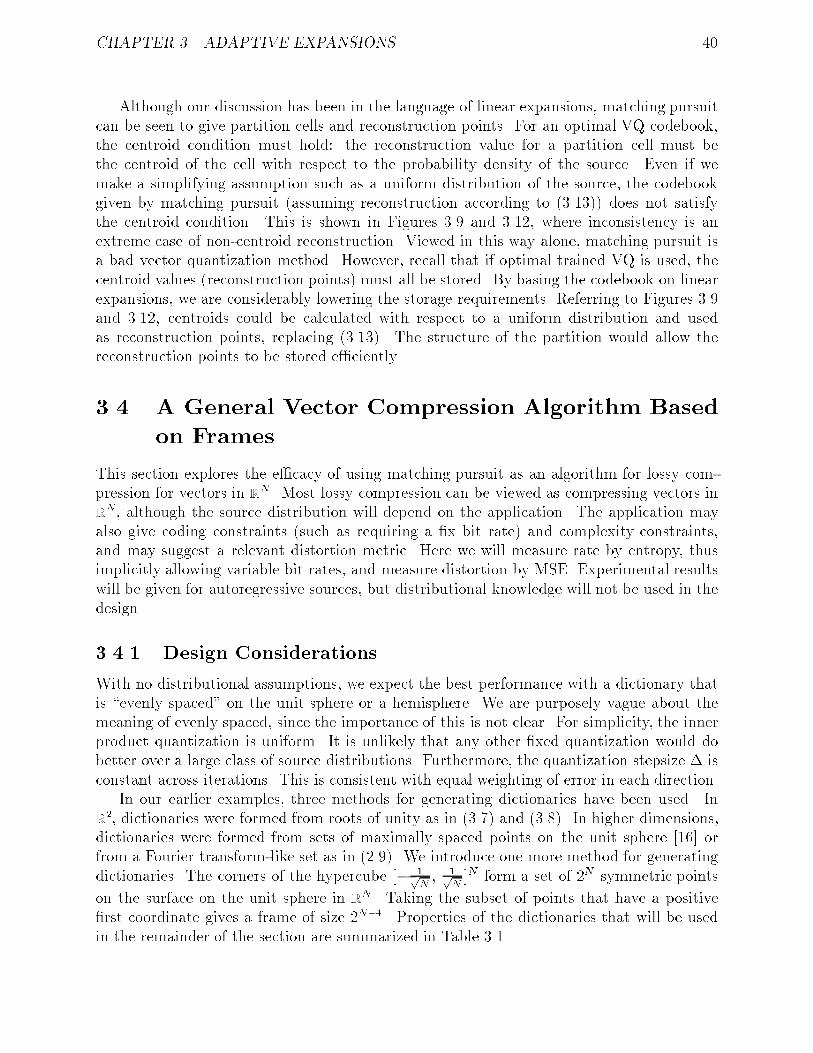
CHAPTER 3. ADAPTIVE EXPANSIONS 40
Although our discussion has been in the language of linear expansions, matching pursuitcan be seen to give partition cells and reconstruction points. For an optimal VQ codebook,the centroid condition must hold: the reconstruction value for a partition cell must bethe centroid of the cell with respect to the probability density of the source. Even if wemake a simplifying assumption such as a uniform distribution of the source, the codebookgiven by matching pursuit (assuming reconstruction according to (3.13)) does not satisfythe centroid condition. This is shown in Figures 3.9 and 3.12, where inconsistency is anextreme case of non-centroid reconstruction. Viewed in this way alone, matching pursuit isa bad vector quantization method. However, recall that if optimal trained VQ is used, thecentroid values (reconstruction points) must all be stored. By basing the codebook on linearexpansions, we are considerably lowering the storage requirements. Referring to Figures 3.9and 3.12, centroids could be calculated with respect to a uniform distribution and usedas reconstruction points, replacing (3.13). The structure of the partition would allow thereconstruction points to be stored e�ciently.
3.4 A General Vector Compression Algorithm Based
on Frames
This section explores the e�cacy of using matching pursuit as an algorithm for lossy com-pression for vectors in RN. Most lossy compression can be viewed as compressing vectors inRN, although the source distribution will depend on the application. The application may
also give coding constraints (such as requiring a �x bit rate) and complexity constraints,and may suggest a relevant distortion metric. Here we will measure rate by entropy, thusimplicitly allowing variable bit rates, and measure distortion by MSE. Experimental resultswill be given for autoregressive sources, but distributional knowledge will not be used in thedesign.
3.4.1 Design Considerations
With no distributional assumptions, we expect the best performance with a dictionary thatis \evenly spaced" on the unit sphere or a hemisphere. We are purposely vague about themeaning of evenly spaced, since the importance of this is not clear. For simplicity, the innerproduct quantization is uniform. It is unlikely that any other �xed quantization would dobetter over a large class of source distributions. Furthermore, the quantization stepsize � isconstant across iterations. This is consistent with equal weighting of error in each direction.
In our earlier examples, three methods for generating dictionaries have been used. InR2, dictionaries were formed from roots of unity as in (3.7) and (3.8). In higher dimensions,
dictionaries were formed from sets of maximally spaced points on the unit sphere [16] orfrom a Fourier transform-like set as in (2.9). We introduce one more method for generatingdictionaries. The corners of the hypercube [� 1p
N; 1p
N]N form a set of 2N symmetric points
on the surface on the unit sphere in RN. Taking the subset of points that have a positive�rst coordinate gives a frame of size 2N�1. Properties of the dictionaries that will be usedin the remainder of the section are summarized in Table 3.1.

CHAPTER 3. ADAPTIVE EXPANSIONS 41
I. DFT-like set given by (2.9)Advantages:� Inner products can be found with an FFT-like algorithm� No need to store dictionaryComment:� Dictionary elements lie in the intersection of the unit sphere with the
plane x1 =1pN.
II. Maximally spaced points on the unit sphere from [16]Disadvantages:� Dictionary must be stored.� Known only for N = 3, 4, 5, and M � 130.
III. Corners of hypercubeAdvantages:� Inner products can be found with additions and subtractions only
(no multiplications).� Can choose ki without calculating any inner products. (Signs of
components of Rif determine which dictionary element should be chosen.)� No need to store dictionaryDisadvantage:� No exibility in choice of M for �xed N .
Table 3.1: Summary of dictionaries used in compression experiments
3.4.2 Experimental Results
The experiments all involve quantization of a zero mean Gaussian AR source with correlationcoe�cient � = 0:9. Source vectors are generated by forming blocks of N samples. Rate ismeasured by summing the (scalar) sample entropies of k0, k1, : : :, kp�1 and c�0, c�1, : : :, d�p�1,where p is the number of iterations of the algorithm.
Figure 3.18 shows the D(R) points obtained using Method I with N = 9. The dictionaryredundancy ratio is r = 8. The dotted curves correspond to varying p, with the leftmostand rightmost curves corresponding to p = 1 and p = 3, respectively. The points along eachdotted curve correspond to various values of �. The solid curve shows the performance ofindependent quantization in each dimension.
The lower boundary of the region bounded below by one or more dotted curves is thebest R-D performance that can be achieved with this dictionary through the choice of pand �. The simulation results show that matching pursuit performs as well or better thanindependent scalar quantization for rates up to about 2.2 bits per source sample.
The simulation described above does not explore the signi�cance of the r parameter.Simulations as above were performed with r ranging from 1 to 256. Redundancy factorsbetween 2 and 8 resulted in the best performance.
A large fraction of the rate comes from coding the indices. In an attempt to exploit thefact that 'ki and 'ki+1 are often nearly orthogonal, experiments were also performed where

CHAPTER 3. ADAPTIVE EXPANSIONS 42
0 0.5 1 1.5 2 2.5 310
−2
10−1
100
Rate (bits/source sample)
Dis
tort
ion
(MS
E)
������ Uniform scalar quantization� � � Matching pursuit data points� � � � �� Attainable with MP
Figure 3.18: R-D performance of matching pursuit quantization with one to three iterations.(N = 9, r = 8, dictionary of type I.)
a single entropy code was applied for (k0; k1; : : : ; kp�1). We refer to this as vector entropycoding of the indices. The entropy coding of the coe�cients remained scalar. Figure 3.19shows the results of experiments with a dictionary of type II. A dictionary of size M = 8is used in R4. The dashed curve results from using matching pursuit with scalar entropycoding of the indices. The dash-dot curve shows the improvement resulting from vectorentropy coding of the indices. The \knees" in these curves correspond to rates at which theoptimal number of iterations changes. For comparison, the solid curve gives the performanceof scalar quantization with scalar entropy coding. Replacing the scalar entropy coding byvector entropy coding gives the dotted curve.
At rates up to about 1.4 bits per source sample, matching pursuit quantization out-performs scalar quantization, even with vector entropy coding. (At these rates, the indexentropy coding method is immaterial because it is best to have only one iteration.) Com-paring to simple scalar quantization with scalar entropy coding, matching pursuit performsabout as well or better over the range of rates considered, up to 3.5 bits per source sample.
This simulation shows that vector entropy coding of indices gives modestly improvedperformance at high rates. At high rates it may at �rst appear that independent quantizationwith vector entropy coding is far superior to other methods, but we must consider thecomplexity involved in the entropy coding. Consider operation at 2 bits/sample. The optimalnumber of matching pursuit iterations is two, so the vector entropy code for the indices has82 = 64 symbols. The entropy codes for �0 and �1 have 20 and 6 symbols, respectively.On the other hand, the vector entropy code for the independently quantized vectors has144 = 38416 symbols. Thus with limited computational resources, the matching pursuitquantizer may be the best choice.
Figure 3.20 shows simulations results using the type III dictionary with N = 8 (M = 27).

CHAPTER 3. ADAPTIVE EXPANSIONS 43
0 0.5 1 1.5 2 2.5 3 3.510
−3
10−2
10−1
Rate (bits/source sample)
Dis
tort
ion
(MS
E) Quantization Coding
������� Scalar Scalar� � � � � � �� Scalar Vector�� �� Matching pursuit Scalar� � � � � Matching pursuit Vector
Figure 3.19: Simulation results for N = 4, M = 8 with dictionary of type II.
The curve types have the same correspondence as in Figure 3.19; the results are qualitativelysimilar.
3.4.3 A Few Possible Variations
The experiments of the previous subsection are the tip of the iceberg in terms of the pos-sible design choices. In this subsection, a few possible variations are presented along withplausibility arguments for their application.
An obvious area to study is the design of dictionaries. For static, untrained dictionaries,issues of interest include not only R-D performance, but also storage requirements, complex-ity of inner product computation, and complexity of largest inner product search.
Looking at the dictionary design problem from a VQ standpoint, the �rst impulse is totrain the dictionary using given training data. Davis [7, Ch. 8] has applied a Lloyd-typealgorithm to optimize a dictionary to minimize
D = E
24 f �L�1Xi=0
�i'ki
235
for some �xed L. We would be interested in the case where the coe�cients are quantized andthe minimization is of D + �R, where R is a rate measure and � is a Lagrange multiplier.The result of such an optimization must have worse performance than a general entropy-constrained VQ design because the matching pursuit algorithm imposes a constraint on thecodebook structure. However, the codebook structure may provide computational advan-tages, so this is worthy of investigation.
Another possibility in dictionary design is to adapt the dictionary by augmenting it withsamples from the source. (Dictionary elements might also be deleted or adjusted.) This

CHAPTER 3. ADAPTIVE EXPANSIONS 44
0 0.2 0.4 0.6 0.8 1 1.2 1.4 1.6 1.8 210
−2
10−1
Rate (bits/source sample)
Dis
tort
ion
(MS
E) Quantization Coding
������� Scalar Scalar� � � � � � �� Scalar Vector�� �� Matching pursuit Scalar� � � � � Matching pursuit Vector
Figure 3.20: Simulation results for N = 8 with dictionary of type III.
would be in the spirit of the Lempel-Ziv algorithm. The decoder would have to be awareof changes in the dictionary, but depending on the nature of the adaptation, this may comewithout a rate penalty.
There is no a priori reason to use the same dictionary at every iteration. Given a piteration estimate, the entropy of kp becomes a limiting factor in adding the results of anadditional iteration. To reduce this entropy, it might be useful to use coarser dictionaries asthe iterations proceed.
In our experiments, we averaged results for quantizing many samples with some �xednumber of iterations. Instead of having a �xed number of iterations, it may be useful touse a stopping criterion based on the energy of the residue. This would create a guaranteedupper bound on the error and might have a favorable impact in an R-D sense.
The experimental results that have been presented are based on entropy coding each c�iindependently of the indices, which are in turn coded either separately or as a vector. Thereare at least three other ways to entropy code:
1. Separately code the pair (ki; �i) for each i;
2. Jointly code all of the indices and jointly code all of the coe�cients;
3. Jointly code all of the indices and coe�cients together.
Joint entropy coding of vectors increases complexity and, because of problems of statisticalsigni�cance, makes simulating very time-consuming. A �nal coding variation, which wasmentioned in x3.3.3, is to discard the indices that correspond to zero quantized coe�cients.This should give a modest reduction in rate.
For a broad class of source distributions, the distributions of the �i's will have somecommon properties because they are similar to order statistics. For example, the probability

CHAPTER 3. ADAPTIVE EXPANSIONS 45
density of �0 will be small near zero. This could be exploited in quantizer design in futurework. Finally, rate-distortion performance might be improved by using quantizers withoverload regions.

Chapter 4
Conclusions
This report has considered the e�ect of coe�cient quantization in overcomplete expansions.Two classes of overcomplete expansions were considered: �xed (frame) expansions and ex-pansions that are adapted to the particular source sample, as given by matching pursuit.
We �rst considered frame expansions. In Theorem 2.2, we proved that a certain type ofsequence of frames approaches a tight frame. Along with being an interesting result in itsown right, this may help in understanding asymptotic properties of frame expansions.
We de�ned the concept of consistency. Along with giving computational methods for�nding consistent estimates, we asserted that consistency is the essential criterion for goodreconstruction. For an expansion with redundancy r, we proved that any reconstructionmethod will give MSE that can be lower bounded by an O(1=r2) expression. Backed byexperimental evidence and a proof of a restricted case, we conjecture that any reconstructionmethod that gives consistent estimates will have an MSE that can upper bounded by anO(1=r2) expression.
After reviewing the matching pursuit algorithm, we showed that it shares some importantproperties with the Karhunen-Lo�eve transform (KLT). For an ellipsoidal source distribution,matching pursuit in some sense �nds the principal axes. Also, it gives better energy com-paction than the KLT.
We showed that the partitions generated by quantizing the coe�cients in matching pur-suit are very intricate. We also showed that consistency is an issue in this type of rep-resentation and gave explicit conditions for consistency. The potential lack of consistencyshows that even though matching pursuit is designed to produce a linear combination to esti-mate a given source vector, optimal reconstruction in the presence of coe�cient quantizationrequires a nonlinear algorithm.
Finally, we considered applying matching pursuit as a general vector compression method.The overhead in using this method is coding the indices of the dictionary elements used.Therefore, in choosing a dictionary size there is a tradeo� between increasing overhead andenhancing the ability to closely match signal vectors with a small number of iterations. Sinceit is a successive approximation method, matching pursuit may be useful in a multiresolutionframework. The inherent hierarchical nature of the representation is amenable to unequalerror protection methods for transmission over noisy channels.
Matching pursuit acts as a \universal transform," giving good energy compaction without
46

CHAPTER 4. CONCLUSIONS 47
knowledge of source statistics. This method gets much of its compression gain from entropycoding. Thus, by coupling it with adaptive and/or universal lossless coding, it could workwell as an adaptive and/or lossless vector compression scheme. We make no optimalityclaims and do not address the issues of \redundancy" and \estimation noise," as de�nedin the universal lossy coding literature. Accordingly, our usage of \universal" refers to theproperties of the transform as opposed to the properties of the entire compression system.
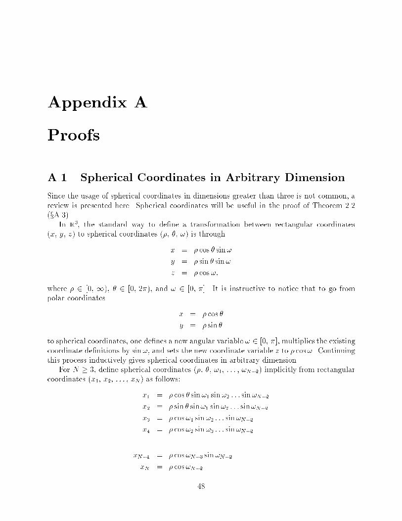
Appendix A
Proofs
A.1 Spherical Coordinates in Arbitrary Dimension
Since the usage of spherical coordinates in dimensions greater than three is not common, areview is presented here. Spherical coordinates will be useful in the proof of Theorem 2.2(xA.3).
In R3, the standard way to de�ne a transformation between rectangular coordinates
(x; y; z) to spherical coordinates (�; �; !) is through
x = � cos � sin!
y = � sin � sin!
z = � cos !;
where � 2 [0; 1), � 2 [0; 2�), and ! 2 [0; �]. It is instructive to notice that to go frompolar coordinates
x = � cos �
y = � sin �
to spherical coordinates, one de�nes a new angular variable ! 2 [0; �], multiplies the existingcoordinate de�nitions by sin!, and sets the new coordinate variable z to � cos!. Continuingthis process inductively gives spherical coordinates in arbitrary dimension.
For N � 3, de�ne spherical coordinates (�; �; !1; : : : ; !N�2) implicitly from rectangularcoordinates (x1; x2; : : : ; xN) as follows:
x1 = � cos � sin!1 sin!2 : : : sin!N�2x2 = � sin � sin!1 sin!2 : : : sin!N�2x3 = � cos!1 sin!2 : : : sin!N�2x4 = � cos!2 sin!3 : : : sin!N�2
...
xN�1 = � cos!N�3 sin!N�2xN = � cos!N�2
48

APPENDIX A. PROOFS 49
Here � 2 [0; 1), � 2 [0; 2�), and !i 2 [0; �] for i = 1; 2; : : : ; N � 2. Note that this can beviewed as a way to parameterize vectors of length � in RN.
By direct calculation, the Jacobian of the transformation is����� @(x1; x2; : : : ; xN)
@(�; �; !1; : : : ; !N�2)
����� = �N�1 sin!1 sin2 !2 : : : sinN�2 !N�2: (A.1)
A.2 Proposition 2.1
A condition for � to span H is that
hf; 'ki = 0 8 k 2 K ) f = 0:
This is immediate from (2.4). It remains to show that the 'k are orthonormal. For anyk 2 K,
k'kk2 =X`2K
jh'k; '`ij2 = k'kk4 +X
`2Knfkgjh'k; '`ij2 :
Now k'kk = 1 implies h'k; '`i = 0 for all ` 6= k.
A.3 Theorem 2.2
Let f�Mg = f'kgMk=1. The corresponding frame operator is given by
F =
266664'T1'T2...'TM
377775 ;so
F �F = ['1 '2 � � � 'M ]
266664'T1'T2...'TM
377775 :The (i; j)th element of 1
MF �F is given by
(1
MF �F )ij =
1
M
MXk=1
(F �)ikFkj =1
M
MXk=1
FkiFkj =1
M
MXk=1
('k)i('k)j;
where ('k)i is the ith component of 'k.First consider the diagonal elements (i = j). Since the ('k)i's are independent, identically
distributed, zero-mean random variables, we �nd that
E�(1
MF �F )ii
�= �2 (A.2)
Var�(1
MF �F )ii
�=
1
M
��4 � M � 3
M � 1�4�; (A.3)

APPENDIX A. PROOFS 50
where �2 = E[('k)2i ] and �4 = E[('k)4i ] [27, x8-1]. For the o�-diagonal elements (i 6= j),
E�(1
MF �F )ij
�= 0 (A.4)
Var�(1
MF �F )ij
�=
1
MEh('k)
2i ('k)
2j
i: (A.5)
Noting that �2 and �4 are independent of M , (A.3) shows that Varh( 1MF �F )ii
i! 0 as
M !1, so ( 1MF �F )ii ! �2 in the mean-squared sense [27, x8-4]. Similarly, (A.4) and (A.5)
show that for i 6= j, ( 1MF �F )ij ! 0 in the mean-squared sense. This completes the proof,
provided �2 = 1N.
We now derive explicit formulas (depending on N) for �2, �4, and Eh('k)
2i ('k)
2j
i. For
notational convenience, we omit the subscript k and use subscripts to identify the componentsof the vector.
To compute expectations, we need an expression for the joint probability density of('1; '2; : : : ; 'N). Denote the n-dimensional sphere centered at the origin with radius � bySn� . Since ' is uniformly distributed on the surface of SN1 , the p. d. f. of ' is given by
f(') =1
cN; 8 ' 2 @SN1 ; (A.6)
where cN is the surface area of SN1 . We can compute cN as follows:
cN =Z@SN
1
dA where dA is a di�erential area element
=Z 2�
0
Z �
0
Z �
0� � �Z �
0sin!1 sin
2 !2 : : : sinN�2 !N�2 d!N�2 : : : d!1d� (A.7)
=�Z 2�
0d���Z �
0sin!1 d!1
��Z �
0sin2 !2 d!2
�� � �
�Z �
0sinN�2 !N�2 d!N�2
�(A.8)
In (A.7) we have parameterized the surface of the sphere with spherical coordinates and usedthe di�erential area segment given by (A.1). Using
Z �
0sin2n � d� =
1 � 3 � 5 � � � (2n� 1)
2 � 4 � � � (2n) � andZ �
0sin2n+1 � d� = 2
2 � 4 � � � (2n)1 � 3 � 5 � � � (2n+ 1)
we can simplify (A.8) to get the following familiar result [3, x1.4]:
cN =N�N=2
(N=2)!=N2N�(N�1)=2(N�1
2 )!
N !: (A.9)
Using (A.6), we can make the following calculation:
�2 = Eh'2i
i= E
h'2N
i

APPENDIX A. PROOFS 51
=Z@SN
1
1
cN'2N dA where dA is a di�erential area element
=1
cN
Z 2�
0
Z �
0� � �
Z �
0(cos!N�2)2 sin!1 sin2 !2 : : : sinN�2 !N�2 d!N�2 : : : d!1d�(A.10)
=1
cN
�Z 2�
0d���Z �
0sin!1 d!1
��Z �
0sin2 !2 d!2
�� � ��Z �
0sinN�3 !N�3 d!N�3
��Z �
0cos2 !N�2 sinN�2 !N�2 d!N�2
�=
�Z �
0sinN�2 !N�2 d!N�2
��1 �Z �
0cos2 !N�2 sinN�2 !N�2 d!N�2
�(A.11)
=
cos!N�2 sinN�1 !N�2
N
����� �0 + 1N
R �0 sinN�2 !N�2 d!N�2R �
0 sinN�2 !N�2 d!N�2
(A.12)
=1
N
In this calculation, (A.10) results from using spherical coordinates and (A.11) follows fromsubstituting (A.8) and cancelling like terms. The simpli�cation (A.12) is due to a standardintegration formula [30, #323]. Similar calculations give
�4 = Eh'4i
i=
3
N(N + 2)(A.13)
and, for i 6= j,
Eh'2i'
2j
i=
1
N(N + 2): (A.14)
A.4 Proposition 2.5
Subtracting
f =MXk=1
(hf; 'ki+ �k) f'kfrom
f =MXk=1
hf; 'kif'kgives
f � f = �MXk=1
�kf'k:Then we can calculate
MSE = E f � f
2 = E
MXk=1
�kf'k 2
= E
" MXi=1
��if'i�!
MXk=1
�kf'k!#
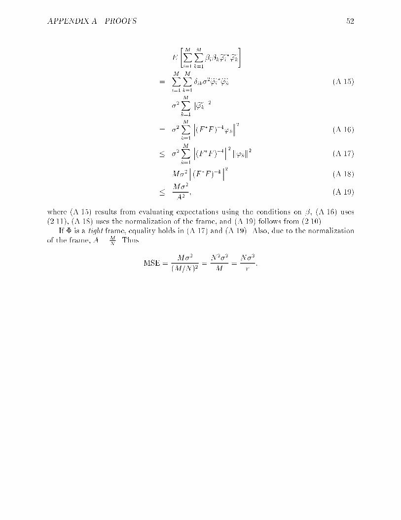
APPENDIX A. PROOFS 52
= E
"MXi=1
MXk=1
��i�kf'i�f'k#
=MXi=1
MXk=1
�ik�2f'i�f'k (A.15)
= �2MXk=1
kf'kk2= �2
MXk=1
(F �F )�1'k 2 (A.16)
� �2MXk=1
(F �F )�1 2 k'kk2 (A.17)
= M�2 (F �F )�1
2 (A.18)
� M�2
A2; (A.19)
where (A.15) results from evaluating expectations using the conditions on �, (A.16) uses(2.11), (A.18) uses the normalization of the frame, and (A.19) follows from (2.10).
If � is a tight frame, equality holds in (A.17) and (A.19). Also, due to the normalizationof the frame, A = M
N. Thus
MSE =M�2
(M=N)2=N2�2
M=N�2
r:

Appendix B
Frame Expansions and Hyperplane
Wave Partitions
This appendix gives an interpretation of frame coe�cients as measurements along di�erentdirections. This allows us to understand the partitioning of RN induced by frame coe�cientquantization without appealing to intersections with the partitioning of RM. We will alsotouch on e�cient coding of frame coe�cients.
Given a frame � = f'kgMk=1, the kth component of y = Fx is yk = hx; 'ki. Thus yk is ameasurement of x along 'k. We can thus interpret y as a vector of M \measurements" of xin directions speci�ed by �. Notice that in the original basis representation of x, we have Nmeasurements of x with respect to the directions speci�ed by the standard basis. Each of theN measurements is needed to �x a point in RN. On the other hand, the M measurementsgiven in y have only N degrees of freedom.
Now let's suppose y is scalar-quantized to give y by rounding each component to thenearest multiple of �. Since yk speci�es the measurement of a component parallel to 'k,yk = (i+ 1
2)� speci�es a hyperplane (N�1 dimensional manifold) perpendicular to 'k. Thusquantization of yk gives a set of parallel hyperplanes spaced by �, called a hyperplane single
wave. The M hyperplane single waves give a partition with a particular structure called ahyperplane wave partition [35].
Examples of hyperplane wave partitions are shown in Figure B.1. Figure B.1(a) showsa frame in R2 composed of three vectors. Suppose x 2 R
2 is speci�ed by quantized innerproducts with each of the three frame vectors. The quantization of the inner product withthe black vector gives the black hyperplane single wave. Similarly for the red and blue framevectors. Figure B.1(b) gives an example with M = 5.
We can now interpret increasing the redundancy r of a frame as increasing the numberof directions in which x is measured. It is well-known that MSE is proportional to �2.Section 2.2.4 presents a conjecture that MSE is proportional to 1=r2. This conjecture can berecast as saying that, asymptotically, increasing directional resolution is as good as increasingcoe�cient resolution. This is shown in Figure B.2. The initial partition is in black, increasingcoe�cient resolution is shown in blue and increasing directional resolution is shown in red.
In x2.2.5 it was mentioned that coding each component of y separately is ine�cient whenr � 1. This can be explained by reference to Figure B.1. Specifying y1 and y2 de�nes a
53

APPENDIX B. FRAME EXPANSIONS AND HYPERPLANE WAVE PARTITIONS 54
(a) (b)
Figure B.1: Examples of hyperplane wave partitions in R2: (a) M = 3. (b) M = 5.
(a) (b)
Figure B.2: Two ways to re�ne a partition: (a) Increasing coe�cient resolution. (b) Increas-ing directional resolution.

APPENDIX B. FRAME EXPANSIONS AND HYPERPLANE WAVE PARTITIONS 55
parallelogram within which x lies. Then there are a limited number of possibilities for y3.(In Figure B.1(a), there are exactly two possibilities. In Figure B.1(b), there are three orfour possibilities.) Then with y1, y2, and y3 speci�ed, there are yet fewer possibilities for y4.If this is exploited fully in the coding, the bit rate should only slightly exceed the logarithmof the number of partition cells.

Appendix C
Lattice Quantization Through Frame
Operations
A lattice � is a set of points consisting of sums of the formPN
k=1 `kvk, where the `k areintegers and the vectors v1, : : : , vN are called a basis of the lattice [3].1 A lattice vector
quantizer is a nearest-neighbor quantizer whose reproduction values form a lattice. Thisappendix establishes a relationship between lattice vector quantization and quantized framerepresentations. We will see that in certain circumstances lattice vector quantization can beachieved by quantized frame expansion followed by operations on discrete variables.
Given a lattice �, the basis is not unique. For example, given a basis fv1; v2; : : : ; vng, wecan form another basis through wi = Tvi, where T is any invertible element ofZn�n. Withoutloss of generality, we will assume that the basis fv1; v2; : : : ; vng is one that minimizes thenorms of the basis elements such that X
i
�ivi
� kvkk (C.1)
for all nontrivial sets of integer coe�cients and for all k.2 Such a basis exists because if (C.1)does not hold for some k, vk can be replaced in the basis by
Pi �ivi.
We would like to describe the partition cells of the lattice vector quantizer associated with�. Since a lattice is invariant to any shift that moves the origin to another lattice point, theVoronoi cells are congruent. For notational convenience, we will consider the region mappedto the origin by the quantizer. Nearest-neighbor encoding implies that the region mappedto the origin is3
R0 =nx 2 RN : kxk < kx� �k 8 � 2 � n f0g
o: (C.2)
This is an in�nite number of half-space constraints. It is shown in [12, xVI. A.] that byremoving redundant constraints (those corresponding to hyperplanes far from the origin),(C.2) can be replaced by a �nite number of constraints. The number of remaining constraints
1It is implicit that the origin is an element of the lattice.2This does not uniquely describe the basis. It is equivalent to choosing a basis which minimizes the
surface area of the fundamental parallelotope. (The volume of the fundamental parallelotope is �xed by �.)See [3, x1.2 of Ch. 1].
3The boundaries can be arbitrarily de�ned.
56

APPENDIX C. LATTICE QUANTIZATION THROUGH FRAME OPERATIONS 57
depends on the lengths of the basis vectors; enforcing (C.1) minimizes the number of hyper-plane constraints. Denote the minimum number of half-space constraints to describe R0 byL. There exists correspondingly �L � � such that
R0 =nx 2 RN : kxk < kx� �k 8 � 2 �L
o:
By symmetry, � 2 �L implies �� 2 �L. Thus the constraints are in the form of L=2 pairsof parallel hyperplanes.
To describe the entire lattice partition requires not only the L hyperplanes, but also thosehyperplanes translated to every lattice point. For some lattices, some of the hyperplanes willcoincide, resulting in a hyperplane wave partition. In these cases, the lattice VQ partitioncells are unions of hyperplane wave partition cells, so lattice VQ can be achieved by aquantized frame expansion followed by the discrete operation of cell unioning.
The familiar hexagonal tiling of R2 is an example of a lattice VQ partitioning that canbe derived from a hyperplane wave partition. Figure C.1 shows the lattice generated byv1 = [
p3 1]T and v2 = [0 2]T . In this case, discarding remote hyperplanes as in [12,
xVI. A.] leaves six half-space constraints for R0. Furthermore,
�6 = fv1; v2; v2 � v1; �v1; �v2; v1 � v2g:
The solid, dashed, and dotted curves correspond to the nearest-neighbor conditions for �v1,�v2, and �(v1 � v2), respectively. The hyperplane wave partition shown in Figure C.1 isequivalent to that generated by a quantized frame expansion with
� =�v22;v1 � v2
2; �v1
2
�and � = 1. (The choice of � is not unique.)
The cells in the hyperplane wave partition are equilateral triangles. By joining the cellsin the hyperplane wave partition in groups of six, one generates the desired lattice partitionof R2. For concreteness, the sequence of operations is shown in Figure C.2. T is a frameexpansion by multiplication with
T =
26640 1p32 �1
2
�p32 �1
2
3775 :Q represents a uniform quantizer which outputs the odd multiple of 1
2nearest to xi
�. Hence
y 2(2k + 1
2: k 2 Z
)3:
Let
V =
8><>:264 �
12�12
12
375 ;264 �
12
12�12
375 ;264 �
121212
375 ;264
12�12�12
375 ;264
12�12
12
375 ;264
1212�12
3759>=>; :

APPENDIX C. LATTICE QUANTIZATION THROUGH FRAME OPERATIONS 58
−4 −3 −2 −1 0 1 2 3 4−4
−3
−2
−1
0
1
2
3
4
Figure C.1: A lattice in R2 shown with the corresponding half-space constraints for nearest-neighbor encoding.
Q
Q
Q
T
x ∈ℜ2 y ∈ℜ3 x ∈ℜ2y ∈ℜ3ˆ ˆ
g U
Figure C.2: Block diagram for hexagonal lattice quantization of R2 through scalar quantiza-tion and discrete operations.
Block g represents a selection function that forms groups of six cells from the hyperplanewave partition associated with T and Q. Denote the output of g by s = [s1 s2]T 2 Z2. Thens is determined by the constraints
9 v 2 V such that v � y =
264 s1s2
�s1 � s2
375 ;and
2s1 + s2 � 0 (mod 3)
s1 + 2s2 � 0 (mod 3):
Finally, x = Us, where
U =
" � �p3�2�p
3
�� 0
#:

Bibliography
[1] K. E. Atkinson, \An Introduction to Numerical Analysis (Second Edition)," Wiley,1989.
[2] A. Buzo, A. H. Gray, Jr. R. M. Gray, and J. D. Markel, \Speech coding based uponvector quantization," IEEE Transactions on Acoustics, Speech and Signal Processing,
Vol. 28, October 1980, pp. 562{574.
[3] J. H. Conway and N. J. A. Sloane, \Sphere Packings, Lattices and Groups," Springer-Verlag, 1988.
[4] Z. Cvetkovi�c and M. Vetterli, \Error Analysis in Oversampled A/D Conversion andQuantization of Weyl-Heisenberg Frame Expansions," submitted to IEEE Transactions
on Information Theory.
[5] I. Daubechies, \The Wavelet Transform, Time-Frequency Localization and Signal Anal-ysis," IEEE Transactions on Information Theory, Vol. 36, No. 5, September 1990, pp.961{1005.
[6] I. Daubechies, \Ten Lectures on Wavelets," SIAM, 1992.
[7] G. Davis, \Adaptive Nonlinear Approximations," Ph.D. dissertation, Mathematics De-partment, NYU, September 1994.
[8] G. Davis, S. Mallat and Z. Zhang, \Adaptive Time-Frequency Approximations withMatching Pursuits," Technical Report 657, Computer Science Department, NYU,March1994.
[9] G. Davis, S. Mallat and M. Avenaleda, \Chaos in Adaptive Approximations," TechnicalReport, Computer Science Department, NYU, April 1994.
[10] R. J. Du�n and A. C. Schae�er, \A class of nonharmonic Fourier series," Transactions
of the American Mathematical Society, Vol. 72, pp. 341{366, 1952.
[11] M. R. Garey and D. S. Johnson, Computers and Intractability: A Guide to the Theory
of NP-Completeness, W. H. Freeman and Company, 1979.
[12] A. Gersho, \On the Structure of Vector Quantizers," IEEE Transactions on Information
Theory, Vol. 28, No. 2, pp. 157{166, March 1982.
59

BIBLIOGRAPHY 60
[13] A. Gersho and R. M. Gray, \Vector Quantization and Signal Compression," KluwerAcademic Publishers, 1992.
[14] V. K. Goyal, M. Vetterli and N. T. Thao, \Quantization of Overcomplete Expansions,"Proceedings of Data Compression Conference (DCC) 1995, pp. 13{22.
[15] C. E. Heil and D. F. Walnut, \Continuous and Discrete Wavelet Transforms," SIAM
Review, Vol. 31, No. 4, December 1989, pp. 628{666.
[16] R. H. Hardin, N. J. A. Sloane and W. D. Smith, \Library of best ways known tous to pack n points on sphere so that minimum separation is maximized," URL:ftp://netlib.att.com/netlib/att/math/sloane/packings/
[17] I. T. Jolli�e, \Principal Component Analysis," Springer-Verlag, 1986.
[18] L. K. Jones, \On a conjecture of Huber concerning the convergence of projection pursuitregression," The Annals of Statistics, Vol. 15, No. 2, pp. 880{882.
[19] T. Kalker and M. Vetterli, \Projection Methods in Motion Estimation and Compensa-tion", Proceedings of IS&T/SPIE 1995.
[20] S. Mallat and Z. Zhang, \Matching pursuits with time-frequency dictionaries," Tech-nical Report 619, Computer Science Department, NYU, August 1993. (Also, IEEE
Transactions on Signal Processing, Vol. 41, No. 12, pp. 3397{3415, December 1993.)
[21] H. S. Malvar, \Signal Processing with Lapped Transforms," Artech House, 1992.
[22] N. J. Munch, \Noise Reduction In Tight Weyl-Heisenberg Frames," IEEE Transactions
on Information Theory, Vol. 38, No. 2, March 1992, pp. 608{616.
[23] R. Ne�, A. Zakhor and M. Vetterli, \Very Low Bit Rate Video Coding Using Match-ing Pursuits," Proceedings of SPIE Conference on Visual Communication and ImageProcessing (VCIP) 1994, Vol. 2308, No. 1, pp. 47{60.
[24] R. Ne�, \Very Low Bit Rate Video Coding Using Matching Pursuits," Masters Thesis,University of California, Berkeley, December 1994.
[25] R. Ne� and A. Zakhor, \Matching Pursuit Video Coding at Very Low Bit Rates,"Proceedings of Data Compression Conference 1995, pp. 411{420.
[26] A. V. Oppenheim and R. W. Schafer, \Discrete-Time Signal Processing," Prentice Hall,1989.
[27] A. Papoulis, \Probability, Random Variables, and Stochastic Processes (Third Edi-tion)," McGraw-Hill, 1991.
[28] T. C. Pati, R. Rezahfar and P. S. Krishnaprasad, \Orthogonal matching pursuit: recur-sive function approximation with applications to wavelet decomposition," Proceedingsof the 27th Asilomar Conference on Signals, Systems and Computers, pp. 40{44, Novem-ber 1993.
BIBLIOGRAPHY 61
[29] K. Ramchandran and M. Vetterli, \Best wavelet packet bases in a rate-distortion sense,"IEEE Transactions on Image Processing, Vol. 2, No. 2, April 1993, pp. 160{175.
[30] Selby, S. M. editor, \Standard Mathematical Tables (Eighteenth Edition)," CRC Press,1970.
[31] G. Strang, \Introduction to Applied Mathematics," Wellesley-Cambridge Press, 1986.
[32] N. T. Thao (Truong-Thao Nguyen), \Deterministic Analysis of Oversampled A/D Con-version and Sigma-Delta Modulation, and Decoding Improvements using ConsistentEstimates," Ph.D. dissertation, Department of Electrical Engineering, Columbia Uni-versity, 1993.
[33] N. T. Thao and M. Vetterli, \Reduction of the MSE in R-times oversampled A/Dconversion from O(1=R) to O(1=R2)," IEEE Transactions on Signal Processing, Vol.42, No. 1, pp. 200{203, January 1994.
[34] N. T. Thao and M. Vetterli, \Deterministic analysis of oversampled A/D conversion anddecoding improvement based on consistent estimates," IEEE Transactions on Signal
Processing, Vol. 42, No. 3, pp. 519{531, March 1994.
[35] N. T. Thao and M. Vetterli, \Lower Bound on the Mean Squared Error in OversampledQuantization of Periodic Signals Using Vector Quantization Analysis," submitted toIEEE Transactions on Information Theory.
[36] M. Vetterli and T. Kalker, \Matching Pursuit for Compression and Application toMotion Compensated Video Coding," Proceedings of International Conference on ImageProcessing (ICIP) 1994.
[37] M. Vetterli and J. Kova�cevi�c, \Wavelets and Subband Coding," Prentice Hall, 1995.
[38] R. Zamir and M. Feder, \Rate-Distortion Performance in Coding Bandlimited Sourcesby Sampling and Dithered Quantization," IEEE Transactions on Information Theory,Vol. 41, No. 1, pp. 141{154, January 1995.
[39] R. Zamir, personal communication, March 29, 1995.
[40] Z. Zhang, \Matching Pursuit," Ph.D. dissertation, NYU, 1993.


