vj kb kh o15085 17210-1-pb

Mathematical Theory and Modeling www.iiste.org

ISSN 2224-5804 (Paper) ISSN 2225-0522 (Online)

Vol.4, No.9, 2014

158

Numerical Solution of Linear Volterra-Fredholm Integro-

Differential Equations Using Lagrange Polynomials

Muna M. Mustafa1 and Adhra’a M. Muhammad

2*

Department of Mathematics, College of Science for Women, University of Baghdad, Baghdad-Iraq

1 E-mail: [email protected] 2 E-mail:[email protected]

Abstract: In this paper, we introduce a numerical method for solving linear Volterra-Fredholm integro-differential Equations

(LVFIDE’s) of the first order. To solve these equations, we consider the polynomial approximation from original

Lagrange polynomial approximation, barycentric Lagrange polynomial approximation, and modified Lagrange

polynomial approximation. Finally, some examples are included to improve the validity and applicability of the

techniques.

Keywords: Linear Volterra-Fredholm integro-differential equation, Original Lagrange polynomial, Barycentric

Lagrange Polynomial, Modified Lagrange polynomial.

1. Introduction:

In recent year, there has been a growing interest in the integro-differential equation which are a combination

of differential and Volterra-Fredholm integral equation. Integro-differential equation play an important role in many

branches of linear and non-linear functional analysis and their applications in the theory of engineering, mechanics,

physics, chemistry, biology, economics, and elctrostations. The mentioned integro- differential equations are usually

difficult to solve analytically, so approximation methods is required to obtain the solution of the linear and non-

linear integro-differential equation [7].

Many researchers studied and discuss the linear Volterra-Fredholm integro-differential equations, E.

Boabolian, Z. Masouri and S. Hatamazadeh-Varmazyar [5] in 2008 construct new direct method to solve non-linear

Volterra-Fredholm integral and integro-differential equation using operational matrix block-pulse functions. AL-

Jubory A. [2] in 2010 introduced some approximation method for solving Volterra-Fredholm integral and integro-

differential equation. M. Dadkah, Kajanj. M. Tavassoli and S. Mahdavi [13] in 2010 used numerical solution of non-

linear Volterra-Fredholm integro-differential equations using Legendre wavelets. R. Mohesn and S. H. Kiasoltani

[14] in 2011 study the solving of non-linear system of Volterra-Fredholm integro-differential equation by using

discrete collocation method. Gherjalar H. D. and M. Hossein [6] in 2012 solved integral and integro-differential

equation by using B-splines function.

Also, Lagrange interpolation polynomial used to solve integral equations. Adibi, H. and Rismani, A. M. [1]

in 2010 applied Legendre-spectral method to solve functional integral equations where the Legendre Gauss points

are used as collocation nodes and Lagrange scheme is employed to interpolate the quantities needed. Shahsavaran, A.

[15] in 2011 presented a numerical method for solving nonlinear VFIE's based upon Lagrange functions

approximations together with the Gaussian quadrature rule and then utilized to reduce the VFIE to the solution of

algebraic equations. Muna M. Mustafa and Iman N. Ghanim [11] in 2014 used Lagrange polynomials to solve linear

Volterra-Fredholm integral equations.

Barycentric Lagrange and modified Lagrange polynomials presented in: Berrut, J.-P. And Trefethen, L. N.

[3] were they discuss Lagrange polynomial interpolation and barycentric Lagrange polynomial interpolation.

Muthumalai, R. K. [12] derived an interpolation formula that generalizes both Newton interpolation formula and

barycentric Lagrange interpolation formula, and Higham, N. J. [8] give an error analysis of the evaluation of

barycentric Lagrange formula and modified formula.

In this work, Lagrange polynomial, and Barycentric Lagrange Polynomial are used to solve LVFIDE's

numerically. The remainder of the paper is organized as follows: the methods of the solution (Lagrange polynomial,

and Barycentric Lagrange Polynomial), test examples are investigated and the corresponding tables are presented.

Finally, the report ends with a brief conclusion.

2. Methods of Solution:

The Linear Volterra-Fredholm integro-differential equation (LVFIDE) of the first order is:

http://www.iiste.org/

mailto:[email protected]



Vol.4, No.9, 2014

159

( ) ( ) ( ) ( ) ∫ ( ) ( ) ∫ ( ) ( ) ( )

Where ( ) ( ) , and ( ) are continuous functions and ( ) is the unknown function to be

determined.

Now, to solve Eq. (1) using original Lagrange polynomial method, barycentric Lagrange Polynomial method, and

modified Lagrange polynomial method; the derivation of the methods are showing as follows:

2.1 Original Lagrange Polynomial Method:

Lagrange interpolation is praised for analytic utility and beauty. The Lagrange approach is in most cases the

method of choice for dealing with polynomial interpolants [4]. This method has the advantage that the values

x0,x1,…,xn need not be equally spaced or taken in consecutive order [9].

Now, define Lagrange formula for a set of n+1 data points {(x0,t0), (x1,t1),…,(xn,tn)}as [4]:

( ) ∑ ( )

( )

Where

( ) ∏( )

( ) ( )

Now, for x = xm then [16]:

( ) ( )

Which that is mean:

( ) {

( )

The error of Lagrange polynomial is [10]:

( ) ( )

( ) ( )( ( )) ( )

Where ( ) ∏ ( ) and ( ) lies in the interval [a, b].

Now, by differentiated (2), we obtain:

(x)=∑

( ) (6)

In order to solve LVFIDE using Lagrange polynomial, we substituting Eq. (6) in Eq. (1), to get:

∑

( ) ( )∑

( ) ( ) ∫ ( ) (

∑

( ))

∫ ( ) (∑

( ))

Therefore:

( ( ) ( ) ( ) ∫

( ) ( ) ∫

( ) ( ) )

+ ( ( ) ( ) ( ) ∫

( ) ( ) ∫

( ) ( ) )

+ ( ( ) ( ) ( ) ∫

( ) ( ) ∫

( ) ( ) )




Vol.4, No.9, 2014

160

+ ( ( ) ( ) ( ) ∫

( ) ( ) ∫

( ) ( ) ) ( )

Putting x=xi, for i=1, 2,…, n , to get a system of n equations, which is:

( )

When .

( ) ( ( ) ( ) ( ) ∫

( ) ( ) ∫

( ) ( ) )

( ) And

( ) ( ) ( ) ∫

( ) ( ) ∫

( ) ( ) )

(9)

For all i, j =1, 2,…, n.

The Algorithm

The numerical solution of LVFIDE's, by using original Lagrange polynomial, is obtained as follows:

Step1:

Put

, u (a) = (initial condition is given)

Step2:

Set , with and , i=0, 1,…, n.

Step3:

Use step 1 and step 2 and Eq. (9) to find dij (Note that for derivative and integral in Eq. (9), we compute the

exact value).

Step4:

Compute using Eq. (8) (Note that for integral in Eq. (8), we compute the exact value).

Step5:

Solve the system Eq. (7) using step3 and step4 and Gaussian Elimination Method.

2.2 Barycentric Lagrange Polynomial Method:

Barycentric interpolation is not new, but most students, most mathematical scientists, and even many

numerical analysis do not know about it [4].

Now, introduce Barycentric Lagrange formula for a set of n+1 data points{(x0,t0),(x1,t1) ,…, (xn,tn)}as [3]:

( )

∑

∑

( )

Where

∏ ( )

( )

And, the error for Barycentric Lagrange polynomial is [12]:

( ) ( ) ( )( ( ))

( ) ( )

Where

( ) ∏( ) ( )




Vol.4, No.9, 2014

161

Now, putting:

(x)=∑ ( ) (14)

And, the derivative for (x)

(x) =∑ ( ) (15)

In order to solve LVFIDE using barycentric Lagrange polynomial, we substituting Eq’s. (14) and (15) in Eq.

(1), to get:

∑ ( )

( )∑ ( )

( ) ∫ ( ) (

∑ ( )

)

∫ ( ) (∑ ( )

)

Therefore:

( ( ) ( ) ( ) ∫

( ) ( ) ∫

( ) ( ) )

+ ( ( ) ( ) ( ) ∫

( ) ( ) ∫

( ) ( ) )

+ ( ( ) ( ) ( ) ∫

( ) ( ) ∫

( ) ( ) )

+ ( ( ) ( ) ( ) ∫

( ) ( ) ∫

( ) ( ) ) ( )

Putting x=xi, for i=1, 2,…, n, to get a system of n equations, which is:

( )

Where .

( ) ( ( ) ( ) ( ) ∫

( ) ( ) ∫

( ) ( ) )

( )

And

( ) ( ) ( ) ∫

( ) ( ) ∫

( ) ( )

(18)

For all i, j =1, 2,…, n.

The Algorithm

The numerical solution of LVFIDE's, by using barycentric Lagrange polynomial, is obtained as follows:

Step1:

Put


Step2:

Set , with and , i=0, 1,…, n.

Step3:

Use step 1 and step 2 and Eq. (18) to find dij (Note that for derivative and integral in Eq. (18), we compute

The exact value).

Step4:


Step5:





Vol.4, No.9, 2014

162

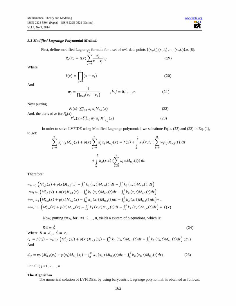
2.3 Modified Lagrange Polynomial Method:

First, define modified Lagrange formula for a set of n+1 data points {(x0,t0),(x1,t1) ,…, (xn,tn)}as [8]:

( ) ( )∑

( )

Where

( ) ∏( ) ( )

And

∏ ( )

( )

Now putting

(x)=∑ ( ) (22)

And, the derivative for (x)

(x)=∑

( ) (23)

In order to solve LVFIDE using Modified Lagrange polynomial, we substitute Eq’s. (22) and (23) in Eq. (1),

to get:

∑

( ) ( )∑

( ) ( ) ∫ ( ) (

∑

( ))

∫ ( ) (∑ ( )

)

Therefore:

( ( ) ( ) ( ) ∫

( ) ( ) ∫

( ) ( ) )

+ ( ( ) ( ) ( ) ∫

( ) ( ) ∫

( ) ( ) )

+ ( ( ) ( ) ( ) ∫

( ) ( ) ∫

( ) ( ) )

+ ( ( ) ( ) ( ) ∫

( ) ( ) ∫

( ) ( ) ) ( )

Now, putting x=xi, for i =1, 2,…, n, yields a system of n equations, which is:

( )

Where .

( ) ( ( ) ( ) ( ) ∫

( ) ( ) ∫

( ) ( ) ) ( )

And

( ( ) ( ) ( ) ∫

( ) ( ) ∫

( ) ( ) ) (26)

For all i, j =1, 2,…, n.

The Algorithm The numerical solution of LVFIDE's, by using barycentric Lagrange polynomial, is obtained as follows:




Vol.4, No.9, 2014

163

Step1:

Put


Step2:

Set , with and , i=0,1,…,n.

Step3:

Use step1, step2 and Eq. (26) to find dij (Note that for derivative and integral in Eq. (26), we

Compute the exact value).

Step4:


Step5:


3. Test Examples:

In this section, we give some of the numerical examples to illustrate the above methods for solving the

LVFIDE's of the first order.

The exact solution is known and used to show that the numerical solution obtained with our methods is correct.

We used MATLAB v 7.6 to solve the examples.

Example 1: Consider the LVFIDE:

( ) ( ) ( ) ∫( ) ( ) ∫( ) ( ) ( )

Where ( ) ( ) ( ) ( ) ( ) ( ) ( )

With the exact solution ( ) ( ).

Tables 1 and 2 represent the absolute error by using Lagrange polynomial, Barycentric Lagrange polynomial,

and Modified Lagrange polynomial with n=5 and n=8 respectively, where ||err||∞is the maximum absolute error, and

R.T. represent the running time.

Table (1)

The Absolute Error of Example 1 by using Lagrange polynomial, Barycentric

Lagrange polynomial, and Modified Lagrange polynomial with n=5

x

Lagrange approximation

Error

Barycentric Lagrange

approximation Error

Modified Lagrange

approximation Error

0.2 .2143244199.192.2e-005 2.391765344289532e-005 2.391765344167407e-005

0.4 2.857260188393607e-005 2.857260188426913e-005 2.857260188426913e-005

0.6 3.408742998700642e-005 3.408742998722847e-005 3.408742998711745e-005

0.8 12.3.1.4.414214.1e-005 3.818385864007290e-005 3.818385863973983e-005

1 92.44492.4.9.2.21e-005 4.299947868502407e-005 4.299947868469101e-005

||err||∞ 4.299947868480203e-005 4.299947868502407e-005 4.299947868469101e-005

R.T. 4.123351239158373e000 1.250613505479534e+001 3.464698443517950e+000




Vol.4, No.9, 2014

164

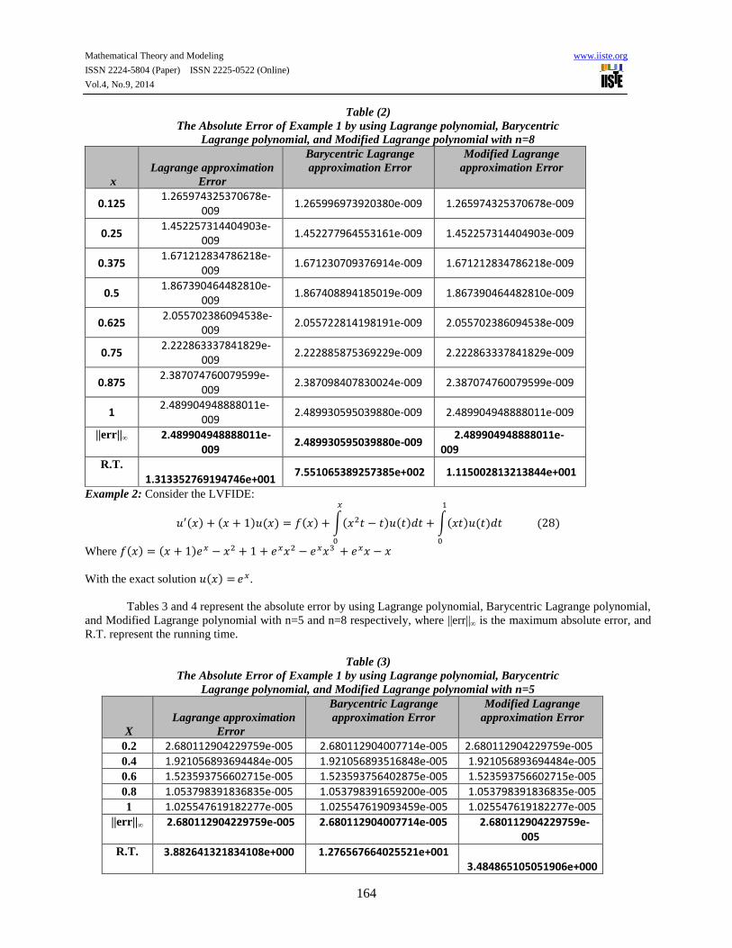
Table (2) The Absolute Error of Example 1 by using Lagrange polynomial, Barycentric


x


Error


approximation Error

Modified Lagrange

approximation Error

0.125 1.265974325370678e-

009 1.265996973920380e-009 1.265974325370678e-009

0.25 1.452257314404903e-

009 1.452277964553161e-009 1.452257314404903e-009

0.375 1.671212834786218e-

009 1.671230709376914e-009 1.671212834786218e-009

0.5 1.867390464482810e-

009 1.867408894185019e-009 1.867390464482810e-009

0.625 2.055702386094538e-

009 2.055722814198191e-009 2.055702386094538e-009

0.75 2.222863337841829e-

009 2.222885875369229e-009 2.222863337841829e-009

0.875 2.387074760079599e-

009 2.387098407830024e-009 2.387074760079599e-009

1 2.489904948888011e-

009 2.489930595039880e-009 2.489904948888011e-009

||err||∞ 2.489904948888011e-009

2.489930595039880e-009 2.489904948888011e-009

R.T. 1.313352769194746e+001

7.551065389257385e+002 1.115002813213844e+001

Example 2: Consider the LVFIDE:

( ) ( ) ( ) ( ) ∫( ) ( ) ∫( ) ( ) ( )

Where ( ) ( )

With the exact solution ( ) .

Tables 3 and 4 represent the absolute error by using Lagrange polynomial, Barycentric Lagrange polynomial,

and Modified Lagrange polynomial with n=5 and n=8 respectively, where ||err||∞ is the maximum absolute error, and

R.T. represent the running time.

Table (3)



X


Error


approximation Error

Modified Lagrange

approximation Error

0.2 2.680112904229759e-005 2.680112904007714e-005 2.680112904229759e-005

0.4 1.921056893694484e-005 1.921056893516848e-005 1.921056893694484e-005

0.6 1.523593756602715e-005 1.523593756402875e-005 1.523593756602715e-005

0.8 1.053798391836835e-005 1.053798391659200e-005 1.053798391836835e-005

1 1.025547619182277e-005 1.025547619093459e-005 1.025547619182277e-005

||err||∞ 2.680112904229759e-005 2.680112904007714e-005 2.680112904229759e-005

R.T. 3.882641321834108e+000 1.276567664025521e+001 3.484865105051906e+000




Vol.4, No.9, 2014

165

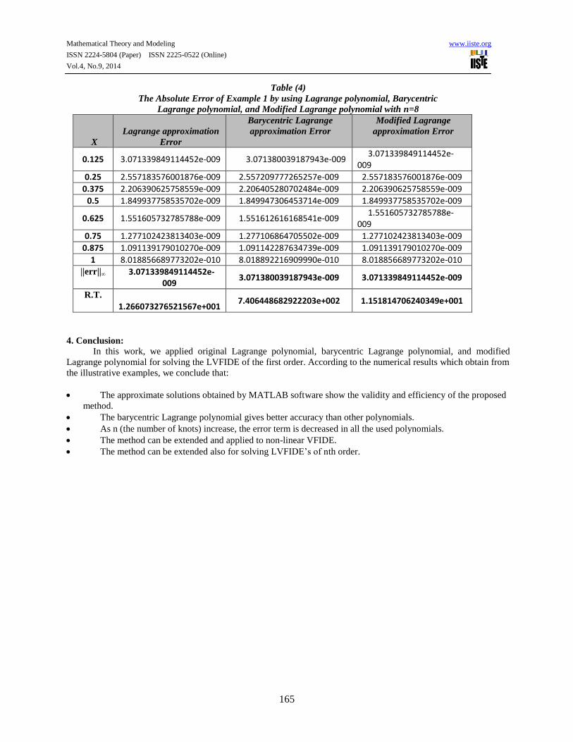
Table (4)



X


Error


approximation Error

Modified Lagrange

approximation Error

0.125 3.071339849114452e-009 3.071380039187943e-009 3.071339849114452e-009

0.25 2.557183576001876e-009 2.557209777265257e-009 2.557183576001876e-009

0.375 2.206390625758559e-009 2.206405280702484e-009 2.206390625758559e-009

0.5 1.849937758535702e-009 1.849947306453714e-009 1.849937758535702e-009

0.625 1.551605732785788e-009 1.551612616168541e-009 1.551605732785788e-009

0.75 1.277102423813403e-009 1.277106864705502e-009 1.277102423813403e-009

0.875 1.091139179010270e-009 1.091142287634739e-009 1.091139179010270e-009

1 8.018856689773202e-010 8.018892216909990e-010 8.018856689773202e-010

||err||∞ 3.071339849114452e-009

3.071380039187943e-009 3.071339849114452e-009

R.T. 1.266073276521567e+001

7.406448682922203e+002 1.151814706240349e+001

4. Conclusion:

In this work, we applied original Lagrange polynomial, barycentric Lagrange polynomial, and modified

Lagrange polynomial for solving the LVFIDE of the first order. According to the numerical results which obtain from

the illustrative examples, we conclude that:

The approximate solutions obtained by MATLAB software show the validity and efficiency of the proposed

method.

The barycentric Lagrange polynomial gives better accuracy than other polynomials.

As n (the number of knots) increase, the error term is decreased in all the used polynomials.

The method can be extended and applied to non-linear VFIDE.

The method can be extended also for solving LVFIDE’s of nth order.




Vol.4, No.9, 2014

166

References:

[1] Adibi, H.; Rismani, A.M.; "Numerical Solution to a Functional Integral Equations Using the Legendre-spectral

Method"; Australian Journal of Basic and Applied Sciences, 4(3), 481-486, 2010.

[2] Al-Jubory, A.; "Some Approximation Methods for Solving Volterra-Fredholm Integral and Integro- Differential

Equations"; Ph.D. Thesis, University of Technology, 2010.

[3] Berrut, J.-P.; Trefethen, L. N.; "Barycentric Lagrange interpolation"; SIAM Review, 46, 3, 501-517, 2004.

[4] Burden, R. L.; Faires, J. D.; "Numerical Analysis"; Ninth Edition, Brooks/Cole, Cengage Learing, 2010.

[5] E. Babolian, Z. Masouri and S. Hatamzadeh-Varmazyar,"New Direct Method to Solve Non-linear Volterra-

Fredholm Integral and integro-differential equation Using operational matrix with Block-pulse Functions", 8, 59-79,

2008.

[6] Gherjalar H. D. and H. Mohammadikia; "Numerical Solution of functional integral and integro-differential

equations by using B-Splines ", Applied Mathematics, 3, 1940-1944, 2012.

[7] Huesin J., Omar A., and AL-shara S., "Numerical solution of linear integro-differential equations", Journal of

Mathematics and statistics, 4, 4, 250-254, 2008.

[8] Higham, N. J. ; "The numerical stability of Barycentric Lagrange interpolation"; IMA Journal of Numerical

Analysis, 24, 547–556, 2004.

[9] Karris, S.T.;"Numerical Analysis Using MATLAB and Excel"; third edition, Orchard Publications, 2007.

[10] Kub´ıˇcek, M.; Janovsk´a, D.; Dubcov , M.; Miroslava Dubcov ; "Numerical Methods and Algorithms";

VˇSCHT Praha, 2005.

[11] Muna M. Mustafa and Iman N. Ghanim; " Numerical Solution of Linear Volterra-Fredholm Integral Equations

Using Lagrange Polynomials"; Mathematical Theory and Modeling, 4, 5, 2014.

[12] Muthumalai, R. K.; "Note on Newton Interpolation Formula"; Int. Journal of Math. Analysis, 6, 50, 2459-2465,

2012.

[13] M. Dadkhah, Kajani M.T., and S. Mahdavi; "Numerical Solution of non-linear Fredholm-Volterra integro-

differential equations using Legendre wavelets"; ICMA 2010.

[14] M. Rabbani and S. H. Kiasodltani; "Solving of non-linear system of Volterra-Fredholm integro-differential

equations by using discrete collocation method "; 3, 4, 382-389, 2011

[15] Shahsavaran, A.; "Lagrange Functions Method for solving Nonlinear Hammerstein Fredholm- Volterra Integral

Equations"; Applied Mathematical Sciences, 5, 49, 2443-2450, 2011.

[16] Yang, W.Y.; Cao, W.; Chung, T.-S.; Morris, J.; "Applied Numerical Methods Using MATLAB"; John Wiley

and Sons, Inc., 2005.


The IISTE is a pioneer in the Open-Access hosting service and academic event

management. The aim of the firm is Accelerating Global Knowledge Sharing.

More information about the firm can be found on the homepage:

http://www.iiste.org

CALL FOR JOURNAL PAPERS

There are more than 30 peer-reviewed academic journals hosted under the hosting

platform.

Prospective authors of journals can find the submission instruction on the

following page: http://www.iiste.org/journals/ All the journals articles are available

online to the readers all over the world without financial, legal, or technical barriers

other than those inseparable from gaining access to the internet itself. Paper version

of the journals is also available upon request of readers and authors.

MORE RESOURCES

Book publication information: http://www.iiste.org/book/

IISTE Knowledge Sharing Partners

EBSCO, Index Copernicus, Ulrich's Periodicals Directory, JournalTOCS, PKP Open

Archives Harvester, Bielefeld Academic Search Engine, Elektronische

Zeitschriftenbibliothek EZB, Open J-Gate, OCLC WorldCat, Universe Digtial

Library , NewJour, Google Scholar


http://www.iiste.org/journals/

http://www.iiste.org/book/

Date post:	19-Jul-2015
Category:	Engineering
Upload:	engr-m-javaid
View:	40 times
Download:	5 times

vj kb kh o15085 17210-1-pb

Engineering