VLSI cell placement techniques - Utah ECEkalla/phy_des/shahookar-mazumdar-placement-survey.pdf ·...

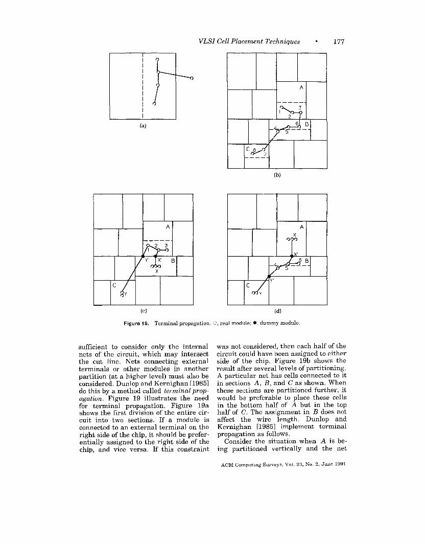
VLSI Cell Placement Techniques

K. SHAHOOKAR AND P. MAZUMDER

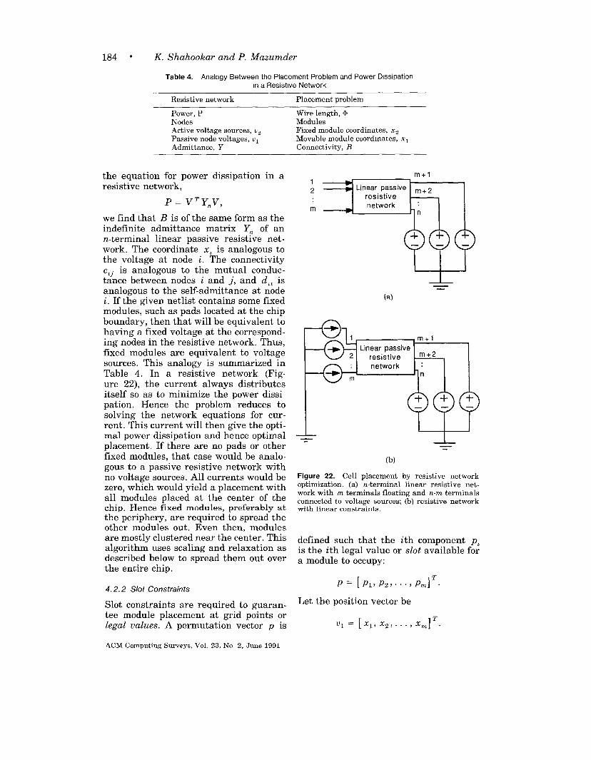
Department of Electrical Engineering and Computer Sc~ence,

University of Michigan, Ann Arbor, Michigan 48109

VLSI cell placement problem is known to be NP complete. A wide repertoire ofheuristic algorithms exists in the literature for efficiently arranging the logic cells ona VLSI chip. The objective of this paper is to present a comprehensive survey of thevarious cell placement techniques, with emphasis on standard ce11and macroplacement. Five major algorithms for placement are discussed: simulated annealing,force-directed placement, rein-cut placement, placement by numerical optimization,and evolution-based placement. The first two classesof algorithms owe their origin tophysical laws, the third and fourth are analytical techniques, and the fifth class ofalgorithms is derived from biological phenomena. In each category, the basic algorithmis explained with appropriate examples. Also discussed are the differentimplementations done by researchers.

Categories and Subject Descriptors: B.7.2 [Integrated Circuits]: DesignAids—placement and routing

General Terms: Design, Performance

Additional Key Words and Phrases: VLSI, placement, layout, physical design, floorplanning, simulated annealing, integrated circuits, genetic algorithm, force-directedplacement, rein-cut, gate array, standard cell

INTRODUCTION

Computer-aided design tools are nowmaking it possible to automate the entirelayout process that follows the circuitdesign phase in VLSI design. This hasmainly been made possible by the use ofgate array and standard cell designstyles, coupled with efficient software

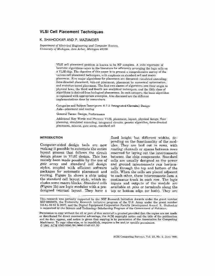
packages for automatic placement androuting. Figure la shows a chip usingthe standard cell layout style, which in-c]udes some macro blocks. Standard cells(Figure lb) are logic modules with a pre-designed internal layout. They have a

fixed height but different widths, de-pending on the functionality of the mod-ules. They are laid out in rows, withrouting channels or spaces between rowsreserved for laying out the interconnectsbetween the chip components. Standardcells are usually designed so the powerand ground interconnects run horizon-tally through the top and bottom of thecells. When the cells are placed adjacentto each other, these interconnects form acontinuous track in each row. The logicinputs and outputs of the module areavailable at pins or terminals along thetop or bottom edge (or both). They are

This research was partially supported by the NSF Research Initiation Awards under the grant numberMIP-8808978, the University Research Initiative program of the U.S. Army under the grant numberDAAL 03-87-K-OO07,and the Digital Equipment Corporation Faculty Development Award. K, Shahookaris supported by the Science and Technology Scholarship Program of the Government of Pakistan.

Permission to copy without fee all or part of this material is granted provided that the copies are not madeor distributed for direct commercial advantage, the ACM copyright notice and the title of the publicationand its date appear, and notice is given that copying is by permission of the Association for ComputingMachinery. To copy otherwise, or to republish, requires a fee and/or specific permission.@1991 ACM 0360-0300/91/0600-0143 $01.50

ACM Computing Surveys, Vol. 23, No. 2, June 1991

144 “ K. Shahoohar and P. Mazumder

CONTENTS

[INTRODUCTIONClassification of Placement AlgorithmsWire length Estimates1 SIMULATED ANNEALING

11 Algorithm12 Operation of Simulated Annealing13 TlmberWolf 321.4 Recent Improvements m Simulated Anneahng

z FORCE.DIRECTED pLAfJEMENT2 1 Force-DwectedPlacement Techniques2.2 Algorithm2,3 Example24 Goto’sPlacement Algorithm25 Analysls

3 PLACEMENT BY PARTITIONING3 1 Breuer’s Algorithms32 Dunlop’s Algorithm and Termmal Propagation33 Quadrlsectlon34 Other Techmques35 Analysls

4, NUMERICAL OPTIMIZATION TECHNIQUES41 Eigenvalue Method42 Resu%lveNetwork Optlmlzatlon43 PROUD: Placement by Block Gauss-Seldel

Optlmlzatlon44 ATLAS: Techmque for Layout Using

Analytlc Shapes45 Algorithm for Block Placement by Size

Optlmlzatlon46 Other Work in This Field

5 PLACEMENT BY THE GENETIC ALGORITHM

5.1 Geme: Genetic Placement Algorlthm5.2 ESP: Evolution-Based Placement Algorlthm53 GASP Genetic Algorlthm for Standard

Cell Placement6 CONCLUSIONACKNOWLEDGMENTSReferences

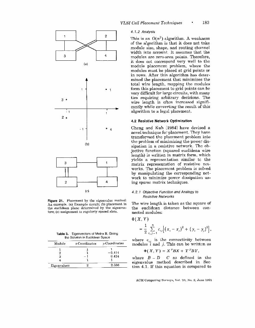
connected by running interconnects orwires through the routing channels. Con-nections from one row to another aredone either through vertical wiringchannels at the edges of the chip or byusing feed-through cells, which are stan-dard height cells with a few intercon-nects running through them vertically.Macro blocks are logic modules not in thestandard cell format, usually larger thanstandard cells, and placed at anyconvenient location on the chip.

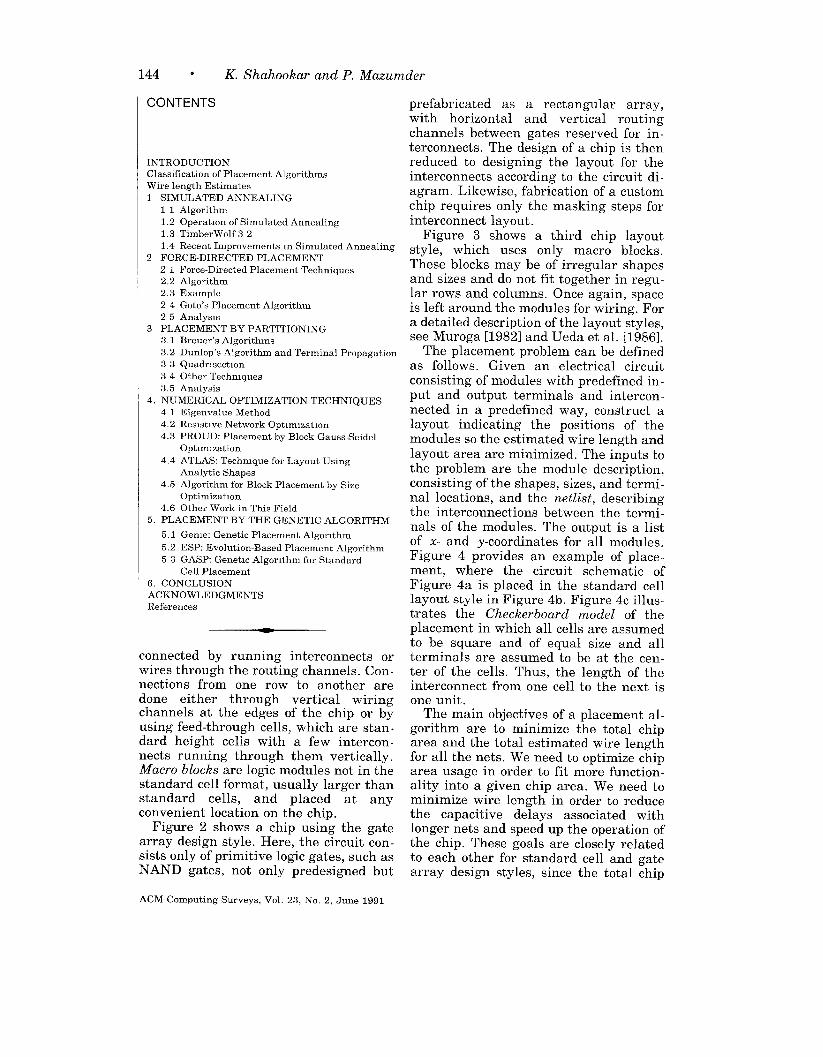
Figure 2 shows a chip using the gatearray design style. Here, the circuit con-sists only of primitive logic gates, such asNAND gates, not only predesigned but

ACM Computing Surveys, Vol 23, No 2, June 1991

prefabricated as a rectangular array,with horizontal and vertical routingchannels between gates reserved for in-terconnects. The design of a chip is thenreduced to designing the layout for theinterconnects according to the circuit di-agram. Likewise, fabrication of a customchip requires only the masking steps forinterconnect layout.

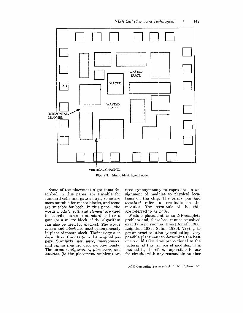
Figure 3 shows a third chip layoutstyle, which uses only macro blocks.These blocks may be of irregular shapesand sizes and do not fit together in regu-lar rows and columns. Once again, spaceis left around the modules for wiring. Fora detailed description of the layout styles,see Muroga [1982] and Ueda et al. [1986].

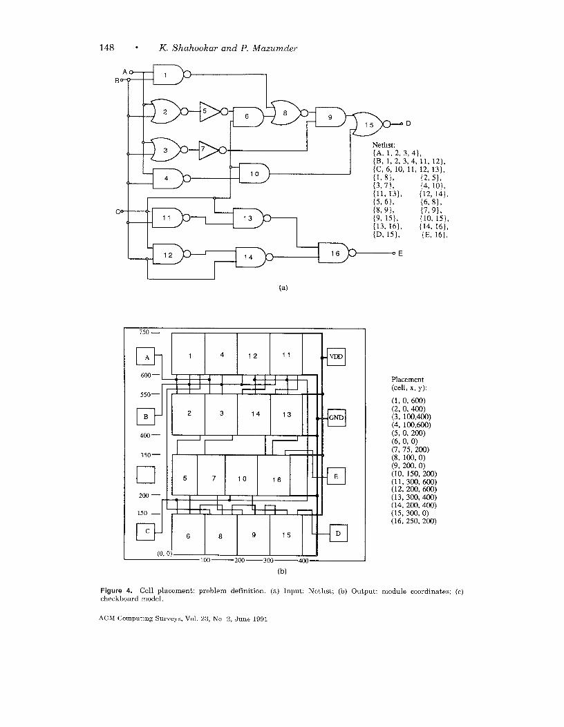
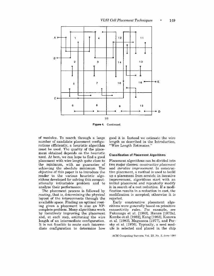
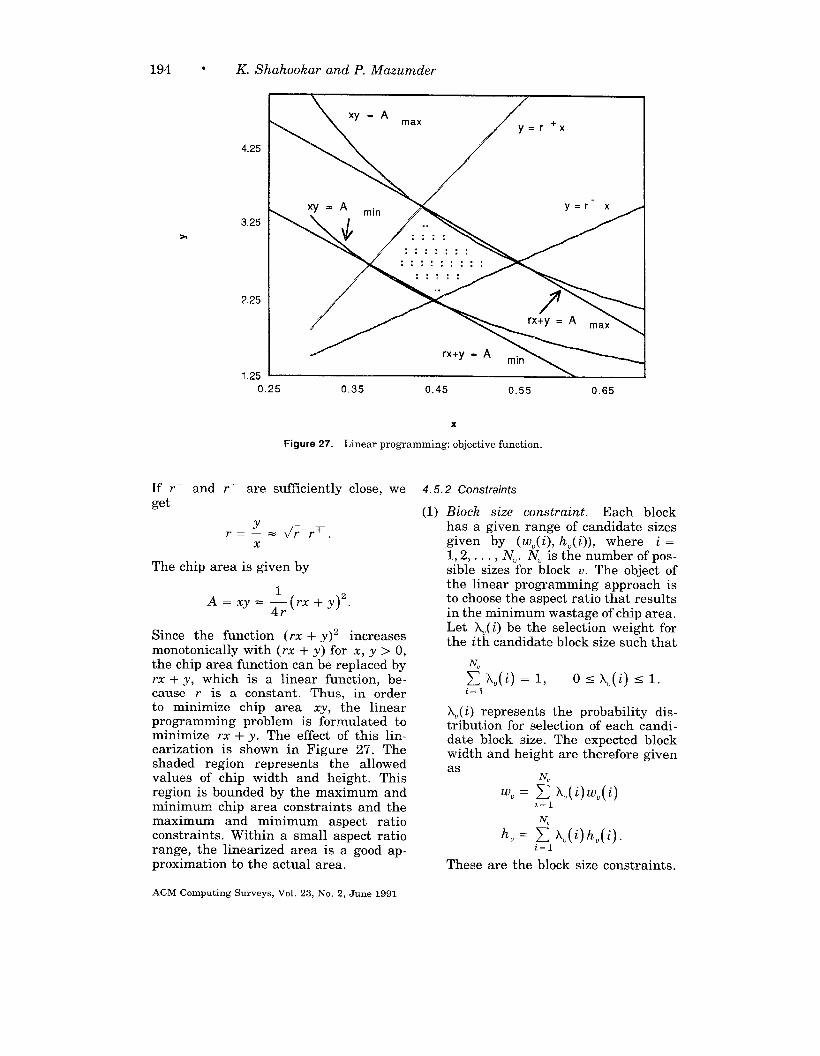
The placement problem can be definedas follows. Given an electrical circuitconsisting of modules with predefined in-put and output terminals and intercon-nected in a predefined way, construct alayout indicating the positions of themodules so the estimated wire length andlayout area are minimized. The inputs tothe problem are the module description,consisting of the shapes, sizes, and termi-nal locations, and the netlist, describingthe interconnections between the termi -nals of the modules. The output is a listof x- and y-coordinates for all modules.Figure 4 provides an example of place-ment, where the circuit schematic ofFigure 4a is placed in the standard celllayout style in Figure 4b. Figure 4C illus-trates the Checkerboard model of theplacement in which all cells are assumedto be square and of equal size and allterminals are assumed to be at the cen-ter of the cells. Thus, the length of theinterconnect from one cell to the next isone unit.

The main objectives of a placement al-gorithm are to minimize the total chiparea and the total estimated wire lengthfor all the nets. We need to optimize chiparea usage in order to fit more function-ality into a given chip area. We need tominimize wire length in order to reducethe capacitive delays associated withlonger nets and speed up the operation ofthe chip. These goals are closely relatedto each other for standard cell and gatearray design styles, since the total chip

Iz E&l

lnlnEam

❑ on ❑ 0[1

❑❑

❑

❑❑

❑

❑

❑

❑

ACM Computing Surveys, Vol, 23, No 2, June 1991

146 . K. Shahookar and P. Mazumder

EIUUEIEIEI❑

clclcl Elncincl nncl Elclcicl ❑ ullclclnnn unnclclcl Elunn Elncl❑ izlclntl nclnclclnclaclcl Elcln

❑tlclclclnlzclclclclnnnn 0000❑ lclnnnclclnnclclclcincl ❑ 00

ATE~aaDtlaaaDa 1317CICICIEIDCI

In ❑ lnnclciclncltlnnclclncl ❑ 00PAD

❑ lnnnnclclclnclnnclclcl ❑ un

HORIZONTAL .tlnnnnnnclclnclnan ❑ oonCHANNEL ~

❑ lclnclnnnciclclnnnn ❑ non

❑

❑

•1

❑ nnnclcl13clnnnDlJnn ❑ un❑ clcinElnElclnElclrJnclcl ❑ un❑ lnnnclclnclclnncluclcl ❑ 00clnnclcllJnnclnclclucln Elan❑ nclnclclnclnElclclclclcl ❑ un❑ lnclclnclnclnnclclclclcl ❑ on❑ lclclclclclnclclnclnucicl ❑ clrl❑ lclclclclclncl ❑ nnncloncln

EIEIEI ❑ onvERTIciLCHANNEL

Figure 2. Gate array layout style

area is approximately equal to the areaof the modules plus the area occupiedbythe interconnect. Hence, minimizing thewire length is approximately equivalentto minimizing the chip area. Inthe macrodesign style, the irregularly sized macrosdonotalwaysfit together, and some spaceis wasted. This plays a major role indetermining the total chip area, andwehave atrade-off between minimizing areaandminimizingthe wire length. In somecases, secondary performance measures,such as the preferential minimization ofwire length of a few critical nets, mayalsobe needed, at the cost ofan increasein total wire length.

cl

•1

❑

•1•1❑

Another criterion for an acceptableplacement is that it should be physically

possible; that is, (1) the modules shouldnot overlap, (2) they should lie withinthe boundaries of the chip, (3) standardcells shouldbe confined to rows inprede-termined positions, and (4) gates in a

gate array should be confined to gridpoints. It is common practiceto define acost function or an objective function,

which consists of the sum of the totalestimated wire length andvariouspenal-ties for module overlap, total chip area,and so on. The goal of the placementalgorithm is to determine a placementwith the minimum possible cost.

ACM Computmg Surveys, Vol. 23, No. 2, June 1991

VLSI Cell Placement Techniques ● 147

HOR

❑ on nan

n L___.d WASI’EI)

mu-=

.$PACE

CHANNEL

❑

n

[n

!

C—3

[1

El

-1❑ pnclncl

❑

•1

❑

❑

❑

•1

VERTICALCHANNELFigure 3. Macro block layout style

Some of the placement algorithms de- used synonymously to represent an as-

scribed in this paper are ‘suitable forstandard cells and gate arrays, some aremore suitable for macro blocks, and somem-e suitable for both. In this paper, thewords module, cell, and element are usedto describe either a standard cell or agate (or a macro block, if the algorithmcan also be used for macros). The wordsmacro and block are used synonymouslyin place of macro block. Their usage alsodepends on the usage in the original pa-pers. Similarly, net, wire, interconnect,and signal line are used synonymously.The terms configuration, placement, andsolution (to the placement problem) are

signment of modules to ‘physical loca-tions on the chip. The terms pin andterminal refer to terminals on themodules. The terminals of the chipare referred to as pads.

Module placement is an NP-completeproblem and, therefore, cannot be solvedexactly in polynomial time [Donath 1980;Leighton 1983; Sahni 1980]. Trying toget an exact solution by evaluating everypossible placement to determine the bestone would take time proportional to thefactorial of the number of modules. Thismethod is, therefore, impossible to usefor circuits with alny reasonable number

ACM Computing Surveys, Vol. 23, No 2, June 1991

148 ● K. Shahookar and P. Mazumder

A

B~

D

<Nethst:

<t [A, 1,2, 3,4),(B, 1,2,3,4, 11, 12),(C, 6, 10, 11, 12, 13),[1,8), (2,5),

() (3,7), (4, lo),(11, 13], (12, 14),(5, 6), {6,8),

co

1 >lb

(8,9), [7,9),1? 13<* (9, 15), {lo, 15),

(13, 16), (14, 16),[D, 15), (E, 16).

12

?

OE

[a)

T 1 I i 1 J i I,

1 1550— I I I

11: v ‘ I I I)

dB 2 3 14 13

b

GND

400 — I II

I II

[I ,

350—I I I I

r II

I

❑ 5 7 10 16!-Kl

E

d’“’”w~ :h150 —

c6 8 9 15 D

(0, o;~ —_ —400

Placement(cell, x, y):

(1, O,600)(2, o,400)(3, 100,400)(4, 100,600)(5, o, 200)(6, O,O)(7, 75, 2(Y3)(8, 100, O)(9, 200, o)(lo, 150, 200)(11, 300, 600)(12, 200, 600)(13, 300, 400)(14, 2CH3,4fw)(15, 300, o)(16, 250, 200)

(b)

Figure 4. Cell placement: problem definition (a) Input: Nethst; (b) Output: module coordinates; (c)checkboard model


VLSI Cell Placement Techniques “ 149

Q o 0 D o

A- - 1 0 4 12 11

0 0

?

6 0“ +

B“ 0 6 0

2 3 14 13

0 0 0

0 0 0 .F

()5 7 10 ?6—

T 7

0

0 .3

co0

6 8 9 15

0 0 0 e 0- * —

[c)

Figure 4. Continued,

of modules. To search throughnumber of candidate dacement

a largeconficu -.

rations efficiently, a heuristic algorithmmust be used. The quality of the place-ment obtained depends on the heuristicused. At best, we can hope to find a goodplacement with wire length quite close tothe minimum, with no guarantee ofachieving the absolute minimum. Theobjective of this paper is to introduce thereader to the various heuristic algo-rithms developed for solving this comput -ationally intractable problem and toanalyze their performance.

The placement process is followed byrouting, that is, determining the physicallayout of the interconnects through theavailable space. Finding an optimal rout-ing given a placement is also an NP-complete problem. Many algorithms workby iteratively improving the placementand, at each step, estimating the wirelength of an intermediate configuration.It is not feasible to route each interme-diate configuration to determine how

good it is. Instead we estimate the wirelength as described in the Introduction,“Wire Length Estimates. ”

Classification of Placement Algorithms

Placement algorithms can be divided intotwo major classes: constructive placementand iterative improvement. In construc-tive placement, a method is used to buildup a placement from scratch; in iterativeimprovement, algorithms start with aninitial placement and repeatedly modifyit in search of a cost reduction. If a modi-fication results in a reduction in cost, themodification is accepted; otherwise it isrejected.

Early constructive placement algo-rithms were generally based on primitiveconnectivity rules. For example, seeFukunaga et al. [1983], Hanan [1972a],Kambe et al. [1982], Kang [1983], Kozawaet al. [19831, Magnuson [19771, and Per-sky et al. [1976]. Typically, a seed mod-ule is selected and placed in the chip


150 “ K. Shahookar and P. Mazumder

layout area. Then other modules are se-lected one at a time in order of theirconnectivity to the placed modules (mostdensely connected first) and are placed ata vacant location close to the placed mod-ules, such that the wire length is mini-mized. Such algorithms are generallyvery fast, but typically result in poor lay-outs. These algorithms are now used forgenerating an initial placement for itera-tive improvement algorithms. The mainreason for their use is their speed. Theytake a negligible amount of computationtime compared to iterative improvementalgorithms and provide a good startingpoint for them. Palczewski [19841 dis-cusses the complexity of such algorithms.More recent constructive placement algo-rithms, such as numerical optimizationtechniques, placement by partitioning,and a force-directed technique discussedhere, yield better layouts but require sig-nificantly more CPU time.

Iterative improvement algorithms typ-ically produce good placements but re-quire enormous amounts of computationtime. The simplest iterative improve-ment strategy interchanges randomly se-lected pairs of modules and accepts theinterchange if it results in a reduction incost [Goto and Kuh 1976; Schweikert1976]. The algorithm is terminated whenthere is no further improvement during agiven large number of trials. An im-provement over this algorithm is re-peated iterative improvement in which theiterative improvement process is re-peated several times with differentinitial configurations in the hope ofobtaining a good configuration in one ofthe trials. Currently popular iterativeimprovement algorithms include simu-lated annealing, the genetic algorithm,and some force-directed placement tech-niques, which are discussed in detail inthe following sections.

Other possible classifications for place-ment algorithms are deterministic algo-rithms and probabilistic algorithms.Algorithms that function on the basis offixed connectivity rules or formulas ordetermine the placement by solving si-multaneous equations are deterministicand will always produce the same result

ACM Computmg Surveys, Vol 23, No 2, June 1991

for a particular placement problem.Probabilistic algorithms, on the otherhand, work by randomly examiningconfigurations and may produce a dif-ferent result each time they are run.Constructive algorithms are usuallydeterministic, whereas iterative im -provement algorithms are usually proba-bilistic.

Wire Length Estimates

To make a good estimate of the wirelength, we should consider the way inwhich routing is actually done by routingtools. Almost all automatic routing toolsuse Manhattan geometry; that is, onlyhorizontal and vertical lines are used toconnect any two points. Further, two lay-ers are used; only horizontal lines areallowed in one layer and only verticallines in the other.

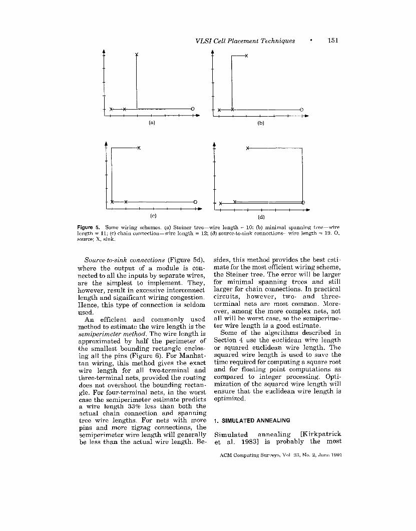
The shortest route for connecting a setof pins together is a Steiner tree (Fig-ure 5a). In this method, a wire can branchat any point along its length. Thismethod is usually not used by routers,because of the complexity of computingboth the optimum branching point, andthe resulting optimum route from thebranching point to the pins. Instead,minimum spanning tree connections andchain connections are the most com-monly used connection techniques. Foralgorithms that compute the Steiner tree:see Chang [1972], Chen [1983], andHwang [1976, 19791.

Minimal spanning tree connections(Figure 5b), allow branching only at thepin locations. Hence the pins are con-nected in the form of the minimal span-ning tree of a graph. Algorithms exist forgenerating a minimal spanning treegiven the netlist and cell coordinates. Anexample of the minimal spanning treealgorithm is Kruskal [1956].

Chain connections (Figure 5c) do notallow any branching at all. Each pin issimply connected to the next one in theform of a chain. These connections areeven simpler to implement than span-ning tree connections, but they result inslightly longer interconnects.


Figure 5.

/x[,,,:.(a)

4x

x Q~~

(c)

Some wiring schemes. (a) Steiner tree-

)

t+(d)

wire length = 10; (b) minimal spanning tree —wirelength = 11; (c) chain c~nnection–wire length = 12; (d) sour;e-to-sink connections–wire length = 19, 0:source; X, sink

Source-to-sink connections (Figure 5d),

where the output of a module is con-nected to all the inputs by separate wires,are the simplest to implement. They,however, result in excessive interconnectlength and significant wiring congestion.Hence, this type of connection is seldomused.

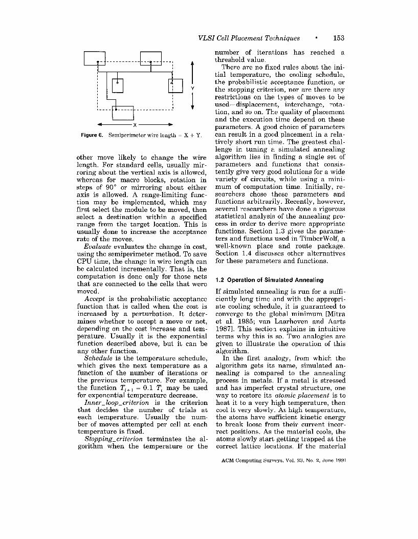
An efficient and commonly usedmethod to estimate the wire length is thesemiperimeter method. The wire length isapproximated by half the perimeter ofthe smallest bounding rectangle enclos-ing all the pins (Figure 6). For Manhat-tan wiring, this method gives the exactwire length for all two-terminal andthree-terminal nets, provided the routingdoes not overshoot the bounding rectan-gle. For four-terminal nets, in the worstcase the semiperimeter estimate predictsa wire length 3370 less than both theactual chain connection and spanningtree wire lengths. For nets with morepins and more zigzag connections, thesemiperimeter wire length will generallybe less than the actual wire length. Be-

sides, this method provides the best esti-mate for the most efficient wiring scheme,the Steiner tree. The error will be largerfor minimal spanning trees and stilllarger for chain connections. In practicalcircuits, however, two- and three-terminal nets are most common. More-over, among the more complex nets, notall will be worst case, so the semiperime -ter wire length is a good estimate.

Some of the algorithms described inSection 4 use the euclidean wire lengthor squared eucliclean wire length. Thesquared wire length is used to save thetime required for computing a square rootand for floating point computations ascompared to integer processing. Opti-mization of the sc[uared wire length willensure that the e uclidean wire length isoptimized.

1. SIMULATED ANNEALING

Simulated annealing [Kirkpatricket al. 1983] is probably the most



well-developed method available for mod-ule placement today. It is very time con-suming but yields excellent results. It isan excellent heuristic for solving anycombinatorial optimization problem, suchas the Traveling Salesman Problem[Randelman and Grest 19861 or VLSI-CAD problems such as PLA folding[Wong et al. 19861, partitioning [Chungand Rao 19861, routing [Vecchi andKirkpatrick 19831, logic minimization[Lam and Delosme 1986], floor planning[Otten and van Ginnekin 1984], or place-ment. It can be considered an improvedversion of the simple random pairwiseinterchange algorithm discussed above.This latter algorithm has a tendency ofgetting stuck at local minima. Suppose,for example, during the execution of thepairwise interchange algorithm, we en-counter a configuration that has a muchhigher cost than the optimum and nopairwise interchange can reduce the cost.Since the algorithm accepts an inter-change only if there is a cost reductionand since it examines only pairwise _in -

tima, we need an algorithm that periodi-cally accepts moves that result in a costincrease. Simulated annealing does justthat.

The basic procedure in simulated an-nealing is to accept all moves that resultin a reduction in cost. Moves that resultin a cost increase are accepted with aprobability that decreases with the in-crease in cost. A parameter T, called thetemperature, is used to control the accep-tance probability of the cost increasingmoves. Higher values of T cause moresuch moves to be accepted. In most im-plementations of this algorithm, the ac-ceptance probability is given byexp (–AC/ T), where AC is the cost in-crease. In the beginning, the tempera-ture is set to a very high value so most ofthe moves are accepted. Then the tem-perature is gradually decreased so thecost increasing moves have less chance ofbeing accepted. Ultimately, the tempera-ture is reduced to a very low value sothat only moves causing a cost reductionare accepted, and the algorithm con-verges to a low cost configuration.

1.1 Algorithm

A typical simulated annealing algorithmis as follows:

PROCEDURE Simulated_ Annealing;initialize;generate random configuration;WHILE stopping. criterion (loop. count, temperature) = FALSE

WHILE inner.loop.criterion = FALSEnew_configuration + perturb(configuration);AC + evaluate(new_con figuration, configuration);IF AC <0 THEN new.configuration + configurationELSE IF accept(AC, temperature) > random(O, 1)

THEN new_configuration - configuration;ENDIF

ENDIFENDWHILEtemperature + schedule(loop_count, temperature);loop_ count + loop_ count + 1;

ENDWHILEEND.

terchanges, there is no way of progress- Perturb generates a random variation

ing further from such a configuration. of the current configuration. This may

The algorithm is trapped at a locally op- include displacing a module to a random

timum configuration, which may be quite location, an interchange of two modules,

poor. Experience shows that this hap- rotation and mirroring within the re -

pens quite often. To avoid such local op - strictions of the layout geometry, or any

ACM Computmg Surveys, Vol 23, No. 2, June 1991

VLSI Cell Placement Techniques g 153

TiI!+:--------------------,~v--t,----------..---------

Y

Figure6. Semiperimeter wire length =X+Y.

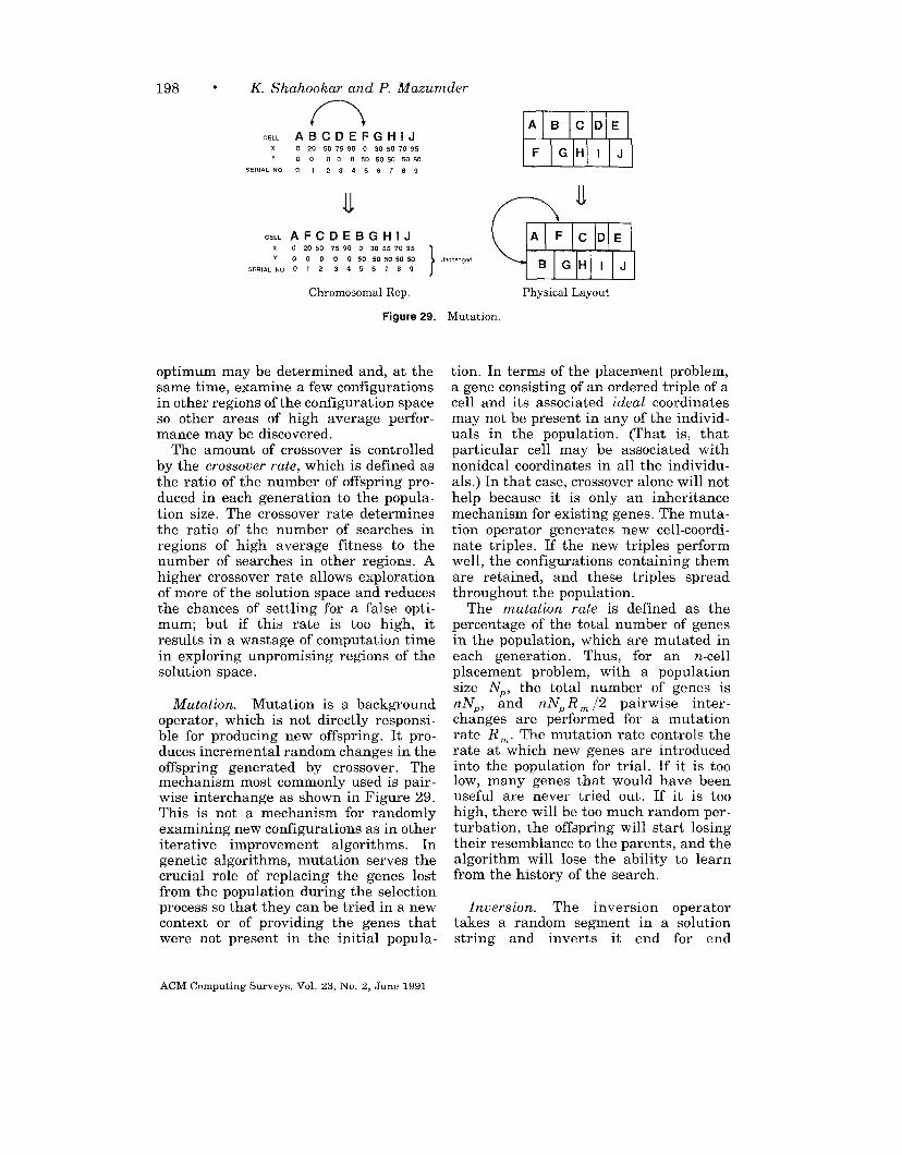
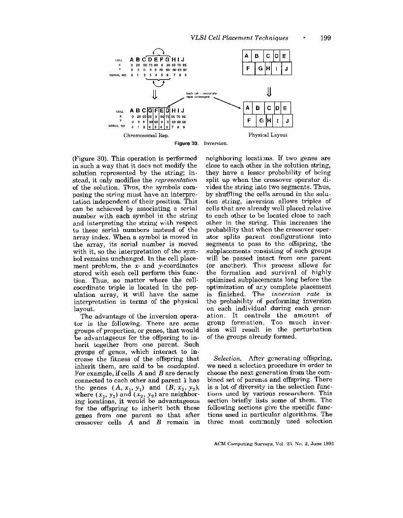
other move likely to change the wirelength. For standard cells, usually mir-rorirw about the vertical axis is allowed.whereas for macro blocks, rotation insteps of 900 or mirroring about eitheraxis is allowed. A range-limiting func-tion may be implemented, which mayfirst select the module to be moved, thenselect a destination within a specifiedrange from the target location. This isusually done to increase the acceptancerate of the moves.

Evaluate evaluates the change in cost,using the semiperimeter method. To saveCPU time, the change in wire length canbe calculated incrementally. That is, thecomputation is done only for those netsthat are connected to the cells that weremoved.

Accept is the probabilistic acceptancefunction that is called when the cost isincreased by a perturbation. It deter-mines whether to acce~t a move or not.depending on the cost increase and tem~perature. Usually it is the exponentialfunction described above. but it can beany other function.

Schedule is the temperature schedule,which gives the next temperature as afunction of the number of iterations orthe previous temperature. For example,the function T,+ ~ = 0.1 T, may be usedfor exponential temperature decrease.

Inner_ loop_ criterion is the criterionthat decides the number of trials ateach temperature. Usually the num-ber of moves attempted per cell at eachtemperature is fixed.

Stopping_ criterion terminates the al-gorithm when the temperature or the

number of iterations has reached athreshold value.

There are no fixed rules about the ini-tial temperature, the cooling schedule,the probabilistic acceptance function, orthe stoplping criterion, nor are there anyrestrictions on the types of moves to beused— displacement, interchange, rota-tion, and so on. The quality of placementand the execution time depend on theseparameters. A good choice of parameterscan result in a good placement in a rela-tively short run time. The greatest chal-lenge in tuning a simulated annealingalgorithm lies in finding a single set ofparameters and functions that consis-tently give very good solutions for a widevariety of circuits, while using a mini-mum of computation time. Initially, re-searchers chose these parameters andfunctions arbitrarily. Recently, however,several researchers have done a rigorousstatistical analysis of the annealing pro-cess in order to derive more appropriatefunctions. Section 1,3 gives the parame-ters and functions used in TimberWolf, awell-known place and route package.Section 1.4 discusses other alternativesfor these parameters and functions.

1.2 Operation of Simulated Annealing

If simulated annealing is run for a suffi-ciently 1ong time and with the appropri-ate cooling schedule, it is guaranteed toconverge to the global minimum [Mitraet al, 1985; van Laarhoven and Aarts1987]. This section explains in intuitiveterms why this is so. Two analogies aregiven to illustrate the operation of thisalgorithm.

In the first analogy, from which thealgorithm gets its name, simulated an-nealing is compared to the annealingprocess in metals. If a metal is stressedand has imperfect crystal structure, oneway to restore its atomic placement is toheat it to a very high temperature, thencool it very slowly. At high temperature,the atoms have sufficient kinetic energyto break loose from their current incor-rect positions. As the material cools, theatoms sl[owly start getting trapped at thecorrect lattice locations. If the material



is cooled too rapidly, the atoms do not geta chance to get to the correct lattice loca-tions and defects are frozen into the crys-tal structure. Similarly, in simulatedannealing at high temperature, there aremany random permutations in the initialconfiguration. These give the cells at in-correct locations a chance to get dis-lodged from their initial position. As thetemperature is decreased, the cells slowlystart getting trapped at their optimumlocations.

In the second analogy, the action ofsimulated annealing is compared to aball in a hilly terrain inside a box [Szu1986]. Without any perturbation, the ballwould roll downhill until it encountereda pit, where it would rest forever al-though the pit may be high above theminimum valley. To get the ball into theglobal minimum valley, the box must beshaken strongly enough so that the ballcan cross the highest peak in its way. Atthe same time, it must be shaken gentlyenough so that once the ball gets into theglobal minimum valley it cannot get out.It must also be shaken long enough sothat there is a high probability of visit-ing the global minimum valley. Thesecharacteristics translate directly into al-gorithm parameters. The strength orgentleness of the vibrations is deter-mined by the probabilistic acceptancefunction and the initial temperature, andthe duration of the vibrations depends onthe cooling schedule and the inner loopcriterion.

1.3 Tim berWolf 3.2

TimberWolf, developed by Carl Sechen

and Sangiovanni-Vincentelli is a widelyused and highly successful place androute package based on simulated an-nealing. Different versions of Timber-Wolf have been developed for placingstandard cells [Sechen 1986, 1988b;Sechen and Sangiovanni-Vincentelli1986], macros [Cassoto et al. 1987], andfloor planning [Sechen 1988al. Version3.2 for standard cells will be describedhere.

TimberWolf does placement and rout-ing in three stages. In the first stage, the

cells are placed so as to minimize theestimated wire length using simulatedannealing. In the second stage, feedthrough cells are inserted as required,the wire length is minimized again, andpreliminary global routing is done. Inthe third stage, local changes are madein the placement wherever possible toreduce the number of wiring tracks re -quired. In the following discussion wewill primarily be concerned with stage 1—placement. Details about the rest ofthe algorithm are given in Sechen [1986,1988b] and Sechen and Sangiovanni-Vincentelli [19861.

The simulated annealing parametersused by TimberWolf are as follows.

1.3.1 Move Generation Function

Two methods are used to generate newconfigurations from the current configu-ration. Either a cell is chosen randomlyand displaced to a random location onthe chip, or two cells are selected ran-domly and interchanged. The perfor-mance of the algorithm was observedto depend upon r, the ratio of dis-placements to interchanges. Exper-imental results given in Sechen andSangiovanni-Vincentelli [1986] indicatethat the algorithm performs best with3~r <8.

Cell mirroring about the horizontalaxis is also done but only when a dis-placement is rejected and only in approx-imately 1O$ZOof those cases selected atrandom. In addition, a temperature-dependent range limiter is used to limitthe distance over which a cell can move.Initially, the span of the range limiter istwice the span of the chip, so for a rangeof high temperatures no limiting is done.The span decreases logarithmically withtemperature:

log TLWV(T) = LwV(TJ-———

log TI

LWH(T) = LwH(TJ~

where LWV(TI) and LWH(TI) are the de-sired initial values of the vertical and



horizontal window span Lw V(T) and

LW~(T), respectively.

1.3.2 Cost Funct/on

The cost function is the sum of threecomponents: the wire length cost, Cl, themodule overlap penalty, Cz, and the rowlength control penalty, C3.

The wire length cost Cl is estimatedusing the semiperirneter method, withweighting of critical nets and indepen-dent weighting of horizontal and verticalwiring spans for each net:

L’l = ~ [x(i) WH(i) +y(i)WV(i)],nets

where %(i) and y(i) are the vertical andhorizontal spans of the net boundingrectangle, and W~( i) and WV(i) are theweights of the horizontal and verticalwiring spans. Critical nets are those thatneed to be optimized more than the rest,or that need to be limited to a certainmaximum length due to propagation de-lay. If they are assigned a higher weight,the annealing algorithm will preferen-tially place the cells connected to thecritical nets close to each other in anattempt to reduce the cost. If the netsstill exceed the maximum length in thefinal placement, their weights can be in-creased and the algorithm run again.

Independent horizontal and verticalweights give the user the flexibility tofavor connections in one direction overthe other. Thus, in double metal technol-ogy, where it is possib [e to stack feedthroughs on top of the cells and they donot take any extra area, vertical spansmay be given preference (lower weight).During the routing phase, these cells areconnected using feed throughs ratherthan horizontal wiring spans through thechannels, and precious channel space isconserved. On the other hand, in chipswhere feed throughs are costly in termsof area, horizontal wiring is preferredand horizontal net spans are given alower weidt. This minimizes the num-ber of fee~throughs required.

The module overlap penalty, Cz,parabolic in the amount of overlap:

C, = W,~ [O(i, j)]2,L#l

is

where 0( i, j) is the overlap between theith and jth cell, and W2 is the weight forthis penalty. It was observed that Czconverges to O for Wa = 1. The parabolicfunction causes large overlaps to be pe-nalized and hence discouraszed more thansmall ones. Although cell overlap is notallowed in the final placement and has tobe removed by shifting the cells slightly,it takes a large amount of computationtime to remove overlap for every pro-posed move. Recall that wire length iscomputed incrementally. If too many cellsare shifted in an attempt to remove over-lap, it would take too much computationto determine the change in wire length.This is whv most al~orithms allow over-lap during”the anne~ling process but pe-nalize it. Overlap only causes a slighterror in the estimated wire lerw-th. Aslong as the overlap is small, th~s errorwill be small. In addition, small overlapstend to get neutralized over several iter-ations. Thus, it is advantageous to ~enal-ize large overlaps more heavily thansmall overlaps by using a quadraticfunction.

The row length control penalty C~ is a

function of the difference between theactual row length and the desired rowlength. It tends to equalize row lengthsby increasing the cost if the rows are ofunequal lengths. Unequal row lengthsresult in wasted space, as shown in Fig-ure la. ‘The penalty is given by

C3=W3~l Ln-iR\,rows

where L,~ is the actual row length, L~ isthe desired row length, and Wa is theweight for this penalty for which the de-fault value of 5 is used. Experimentsshow that the function used provides goodcontrol, with final row lengths within3-5% of the desired value. Results of twoexperiments are given by Sechen andSangiovanni-Vincentelli [19861, showinga reduction in wire length when the rowlength control penalty was introduced.

1.3.3 Inner Loop Criterion

At each temperature, a fixed number ofmoves per cell is attempted. This number


100 0.--K. Shahookar and P. Ma.zumder

900000

800000-

700000-

600000 r , ,0 100 200 300 400 500

Moves per cell

(a)

,.9

4b,.8

No. of mnfigurations exammed,.7

,.6

,.5

,.4

,.3{1

,.2 Recommended no. of moves per cell

,.1.

,.O

0 1000 2000 3000cells

(b)

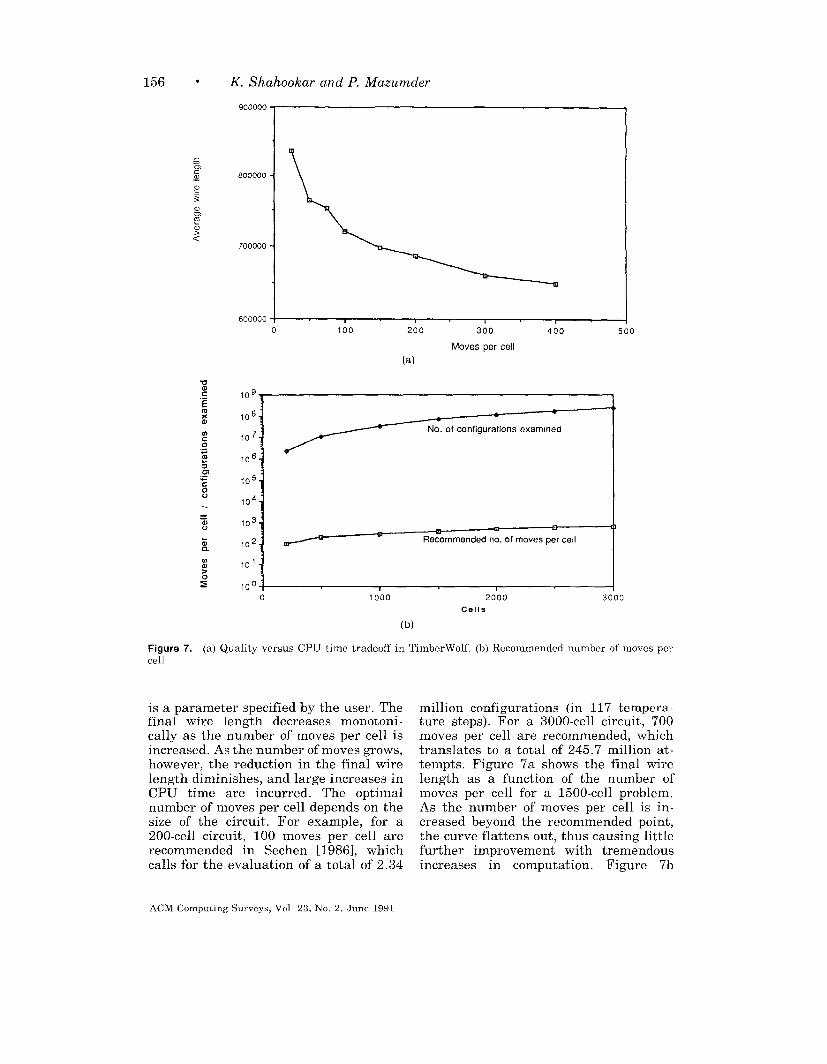
Figure 7. (a) Quality versus CPU time tradeoff in TlmberWolf (b) Recommended number of moves percell

is a parameter specified by the user. Thefinal wire length decreases monotoni-cally as the number of moves per cell isincreased. As the number of moves grows,however, the reduction in the final wirelength diminishes, and large increases inCPU time are incurred. The optimalnumber of moves per cell depends on thesize of the circuit. For example, for a200-cell circuit, 100 moves per cell arerecommended in Sechen [1986], whichcalls for the evaluation of a total of 2.34

million configurations (in 117 tempera-ture steps). For a 3000-cell circuit, 700moves per cell are recommended, whichtranslates to a total of 245.7 million at-tempts. Figure 7a shows the final wirelength as a function of the number ofmoves per cell for a 1500-cell problem.As the number of moves per cell is in-creased beyond the recommended point,the curve flattens out, thus causing littlefurther improvement with tremendousincreases in computation. Figure 7b

ACM Computmg Surveys, Vol 23. No 2, June 1991


,.7

,.6

T,.5

,.4

,.3

,.2

10’

,.O

]\

~:;Lr \~~o 20 40 60 80 100 1

Heration No.

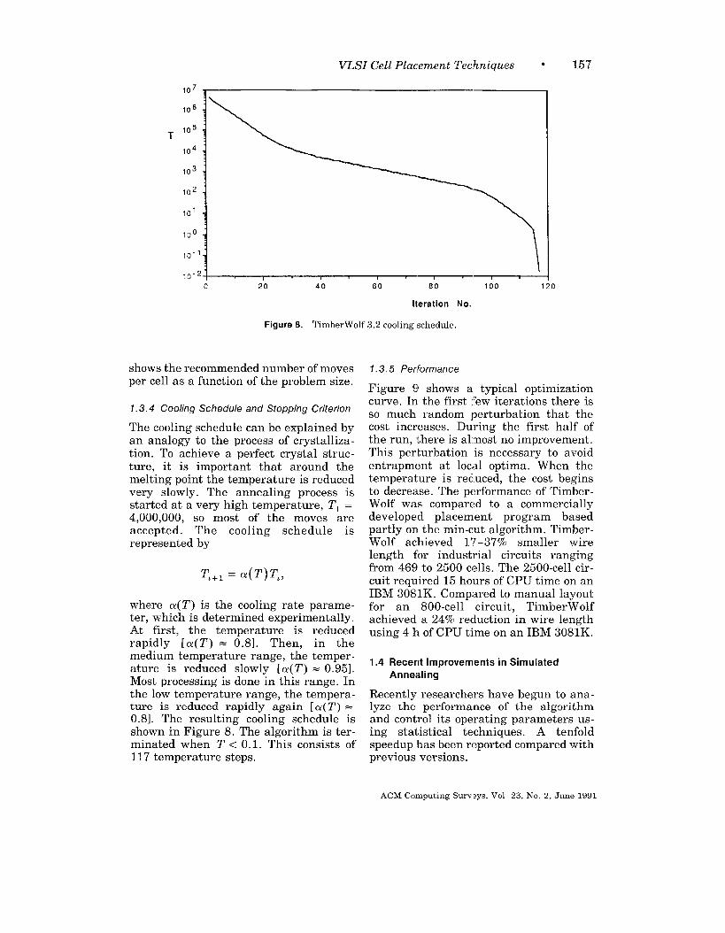
Figure 8. TimberWolf 3.2 cooling schedule.

shows the recommended number of movesper cell as a function of the problem size.

1.3.4 Cooling Schedule and Stopping Criterion

The cooling schedule can be explained byan analogy to the process of crystalliza-tion. To achieve a perfect crystal struc-ture, it is important tl-lat around themelting point the temperature is reducedvery slowly. The annealing process isstarted at a very high temperature, ~1 =4,000,000, so most of the moves areaccepted. The cooling schedule isrepresented by

T2+1= CY(T)~,>

where CY(T) is the cooling rate parame-ter, which is determined experimentally.At first, the temperature is reducedrapidly [a(T) = 0.8]. Then, in themedium temperature range, the temper-ature is reduced slowly [a(T) = 0.95].Most processing is done in this range. Inthe low temperature range, the tempera-ture is reduced rapidly again [Q(T) =0.8]. The resulting cooling schedule isshown in Figure 8. The algorithm is ter-minated when T < 0.1. This consists of117 temperature steps.

o

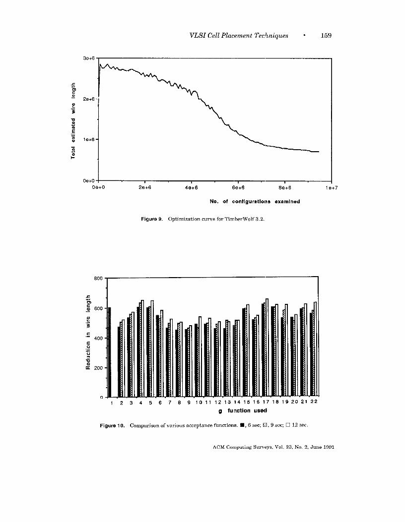
1.3.5 Per~ormance

Figure 9 shows a typical optimizationcurve. In the first few iterations there isso much random perturbation that thecost increases. During the first half ofthe run, there is al,most no improvement.This perturbation is necessary to avoidentrapment at local optima. When thetemperature is reduced, the cost beginsto decrease. The performance of Timber-Wolf was compared to a commerciallydeveloped placement program basedpartly on the rein-cut algorithm. Timber-Wolf achieved 1~-sy’%. smaller wirelength for industrial circuits rangingfrom 469 to 2500 cells. The 2500-cell cir-cuit required 15 hours of CPU time on anIBM 3081K. Compared to manual layoutfor an 800-cell circuit, TimberWolfachieved a 24% reduction in wire lengthusing 4 h of CPU time on an IBM 3081K.

1.4 Recent Improvements in Simulated

Annealing

Recently researchers have begun to ana-lyze the performance of the algorithmand control its operating parameters us-ing statistical techniques. A tenfoldspeedup has been reported compared withprevious versions.



1.4.1 Effect of Probab/1/stic Acceptance

Functions

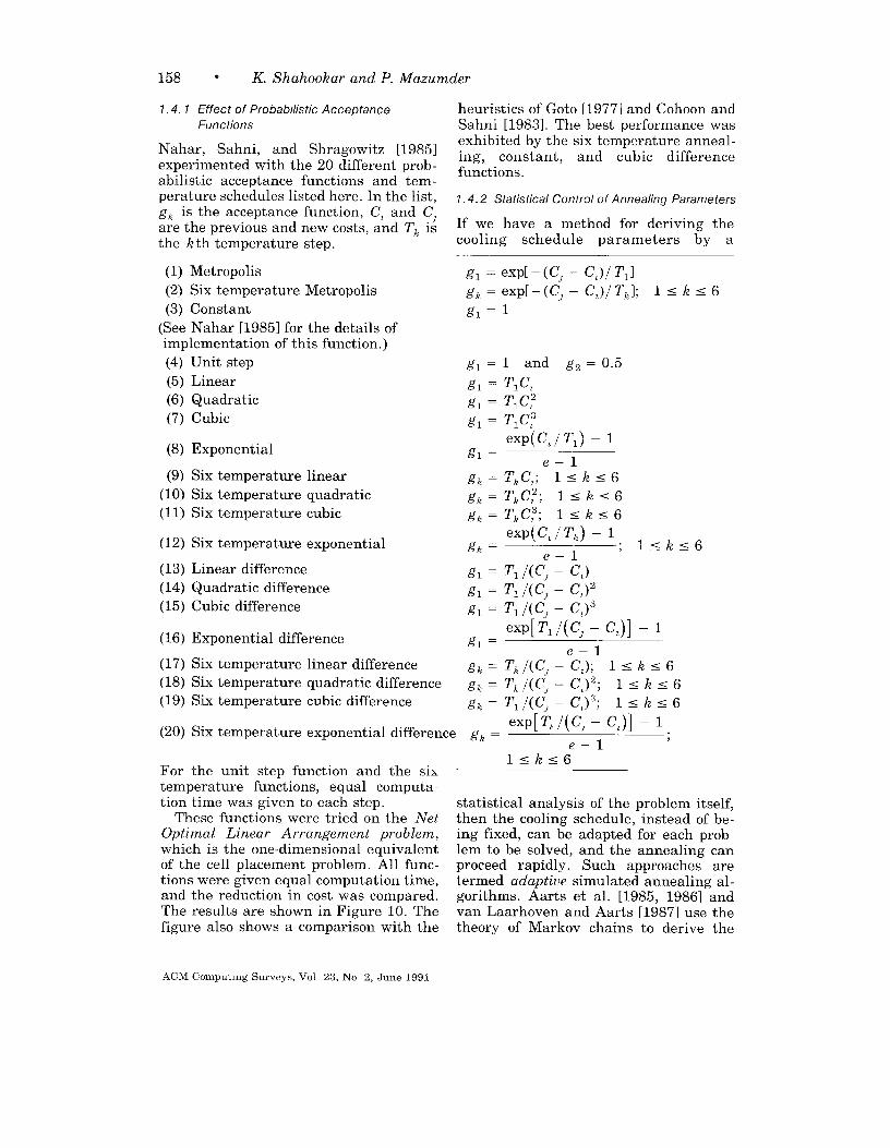
Nahar, Sahni, and Shragowitz [1985]experimented with the 20 different prob-abilistic acceptance functions and tem-perature schedules listed here. In the list,

&?k is the acceptance function, C, and CJare the previous and new costs, and Th isthe k th temperature step.

(1) Metropolis

(2) Six temperature Metropolis

(3) Constant

(See Nahar [19851 for the details ofimplementation of this function.)

(4) Unit step

(5) Linear

(6) Quadratic

(7) Cubic

(8) Exponential

(9) Six temperature linear

(10) Six temperature quadratic

(11) Six temperature cubic

(12) Six temperature exponential

(13) Linear difference

(14) Quadratic difference

(15) Cubic difference

(16) Exponential difference

(17) Six temperature linear difference

(18) Six temperature quadratic difference

(19) Six temperature cubic difference

heuristics of Goto [1977] and Cohoon andSahni [1983]. The best performance wasexhibited by the six temperature anneal-ing, constant, and cubic differencefunctions.

1.4.2 Statistical Control of Annealing Parameters

If we have a method for deriving thecooling schedule parameters by a

gl = exp[–(CJ – Cz)/Tll

gk = exl?–(c~ – 6’,)/ Tk]; 1< k <6

gl=l

exP(cL/Th)–l; ~<k<6gk =

e–1

gl = T, /(cJ – c,)g, = T1 I(C, – C,)2gl = T1/(c, – C,)3

exP[~l/(c, – CL)] – 1gl =e–1

L?k=Tk/(c, -c,); l=k=6

gk=Tk/(cJ–c,)2; l=k=6

L7k=T1/(cJ-c,)3; l=k=6

exp[Tk/(C, – CL)] – 1.(20) Six temperature exponential difference gk =

e–1

For the unit step function and the sixtemperature functions, equal computa-tion time was given to each step.

These functions were tried on the NetOptimal Linear Arrangement problem,which is the one-dimensional equivalentof the cell placement problem. All func-tions were given equal computation time,and the reduction in cost was compared.The results are shown in Figure 10. Thefigure also shows a comparison with the

statistical analysis of the problem itself,then the cooling schedule, instead of be-ing fixed, can be adapted for each prob-lem to be solved, and the annealing canproceed rapidly. Such approaches aretermed adaptiue simulated annealing al-gorithms. Aarts et al. [1985, 1986] andvan Laarhoven and Aarts [1987] use thetheory of Markov chains to derive the



3e+6

s‘g~

2e+6a)&.-

%

ual%E.-Za 1e+6

=z1-

Oe+O

Oe+O 2e+6 4e+6 6e+6

No. of configurations

Figure 9. Optimization curve for TimberWolf 3.2.

8e+6 1e+7

examined

800T———— I

34567 8 910111213141516171619202122

g function ussd

Figure 10. Comparison of various acceptance functions. ■ , 6 see; U, 9 see; ❑ 12 sec.



cooling schedule. Similar expressionswere developed by Huang et al. [1986].

Notation

R = {rl, rz, . . . ,rl~l} is the configura-

tion space, the set of all possible place-ments, where

i is a configuration label, which identi-fies a configuration uniquely,

r, is the ith configuration vector, giv-ing the coordinates of all modules in theith placement,

e, is the ith unit vector in [0, 1] IR I

lR={ilr, eR}={l,2, . . .. i...., IRI}

is the set of configuration labels,C : R + R is the cost function, which as-

signs a real number C(rt) to each config-uration i c lR such that the lower thevalue of C, the better the correspondingconfiguration.

The algorithm can be formulated as asequence of Markov chains, each chainconsisting of a sequence of configurationsfor which the transition probability fromconfiguration i to configuration j is givenby

pwv’z, ifi+j

where P,J is the perturbation probabil-ity, that M, the probability of generatinga configuration j from configuration i

(independent of T); A ,J(T) is the accep-tance probability, that is, the probabil-ity of accepting configuration j if thesystem is in configuration i; and T isthe temperature.

The perturbation probability is chosenas

if J”+ IRL,

where R, is the configuration subspacefor configuration i, which is defined asthe space of all configurations that canbe reached from configuration i by a sin-gle perturbation. This is a uniform prob-ability distribution for all configurationsin the subspace.

The acceptance probability is chosen as

{()–AC,~

A,,(T) = ‘Xp Tif AC,l > 0

1 if ACC~ s O,

where ACZ7 = C(r~) – C(r,). This ex-pression is known as the Metropoliscriterion.

From the theory of Markov chains itfollows that there exists a uni ue

?equilibrium vector q(T) e [0, 1] R Ithat satisfies

for all i e IR: lim e~@(T) = q~(T).L~m

If we start from any configuration, i, andperform L perturbations, with L + co,then the probability of ending up in statej is given by the component qJ( T) of theequilibrium vector. Thus, the equilib-rium vector q(T) gives the probabilitydistribution for the occurrence of eachstate at equilibrium. For the values ofP,J and A ,J(T) given above,

()–AC,tiqj(T) = qO(T)exp

T’

where i. is the label of an optimal con-figuration and qo(T) is a normalizationfactor given by

1%(T) = IRI

()AClok “~exp-yk=l

Further,

lim (e,@(T))J::om-

= J~~_qJ(T)

[

= IROI-’ ifjGIRO

o if J“~IRO,



where R ~ is the set of optimal configura-tions, that is, RO = {r, e R I C(rL) =C(rJ}. Thus, for Markov chains of infi-nite length, the system will achieve oneof the optimal configurations with a uni-form probability distribution, and theprobability of achieving a suboptimalconfiguration is zero.

Initial Temperature. A fixed initialtemperature TI is not used. Instead, theinitial temperature is set so as to achievea desired initial acceptance probability,xo. If ml and mz are the number ofperturbations so far that result in costreduction and cost increase, respectively,and if the m2 cost-increasing perturba-tions are accepted according to theMetropolis criterion, the total number ofconfigurations accepted is ml +mz exp (–AC/T). This gives x. as

ml + mzexp(– AC/T)X. =

ml + m2

This equation can be rewritten to calcu-late the initial temperature from thedesired value of xo:

[( )1

–1

TI = AC(+) invz,xo - ~- Xo)ml ‘

where AC(+) is the average value of allincreases in cost, ignoring cost reduc-tions. The initial system is monitoredduring a number of perturbations beforethe actual optimization process begins.Starting with TI = O, after each pertur-bation a new value of TI is calculatedfrom the above expression.

According to Huang et al. [19861, thesystem is considered hot enough whenT>> a, vvhere u is the standard devia-

tion of the cost function. Hence the start-ing temperature is taken as TI = k u,where k = – 3 /ln( P). This allows thestarting temperature T to be high enoughto accept with probability P a configura-tion whose cost is 3U worse than thepresent one. A typical value of k is 20 forP = 0.9. First, the configuration space isexplored to determine the standard devi -

ation of the cost function; then the start-ing temperature is calculated.

Temperature Decrement. Most otherimplementations used predeterminedtemperature decrements, which are notoptimal for all circuit configurations.Such a cooling schedule leads to variablelength Markov chains. Aarts et al. [19861recommend the use of fixed lengthMarkov chains. This can be achievedusing the foIlowing temperaturedecrement:

( )ln(l + 6)T, ‘1Ti+l =T, l+ sg ,

z

where o, is the standard deviation of thecost function up to the temperature T,,and 6 is a small real number that is ameasure of how close the equilibrium

vectors q. of two successive iterationsare to each other:

Huang et al. [19861 use the average

cost versus log-temperature curve toguide the temperature decrease so thatthe cost decreases in a uniform manner.Hence,

T,AC

()Ti+l = T, exp —

U2 “

This equation has been derived by equat -ing the slope of the annealing curve to02/T2. To maintain quasiequilibrium,the decrease in cost must be less thanthe standard deviation of the cost. ForAC= –Ao, h<l,

T 2+1 ()=Tlexp –3 .u

Typically, A = 0.7. The ratio T,+ ~ / T, isnot allowed to go below a certain lowerbound (typically 0.5) in order to



prevent a drastic reduction in tempera-ture caused by the flat annealing curveat high temperature.

Stopping Criterion. The stopping cri-terion is given by Aarts et al. [19861 as

where e, is a small positivgnumber calledthe stop parameter, and C(TI) is the av-

erage value of the cost function at T1.This condition is based on extrapolating

the smoothed average cost C~(T,) ob-tained during the optimization process.This average is calculated over a numberof Markov chains in order to reduce thefluctuations of ~(T,).

Run-Time Complexity and Experimen-tal Results. The Aarts et al. [1986] algo-rithm has a complexity 0( I R I In I R I),where I R I originates from the length ofthe Markov chains, and the term in I R Iis an upper bound for the number oftemperature steps. The perturbationmechanism can be carefully selected sothat the size of configuration subspacesis polynomial in the number of variablesof the problem. Consequently, the simu-lated annealing algorithm can always bedesigned to be of polynomial time com-plexity in the number of variables.

The Huang et al. [19861 algorithm hasbeen tested on circuits of size 183-800cells. It results in 16–57% saving in CPUtime compared to TimberWolf for approx-imately the same placement quality.CPU times reported are of the order of 9h on a VAX 11/780 for an 800-cell cir-cuit, whereas the same circuit requires11 h with TimberWolf 3.2.

1.4.3 Improved Annealing Algorithm in

TimberWolfSC 4.2

Sechen and Lee [1987] implemented afast simulated annealing algorithm aspart of TimberWolfSC version 4.2, whichis 9–48 times faster than version 3.2, Asa consequence of this algorithm, place-

ment of up to 3000 cells can be done on aMicro VAX II workstation in under 24 hof CPU time. The parameters they useare as follows.

Cost Function. The standard costfunction consisting of semiperimeter wirelength, with adjustable weights for verti-cal and horizontal nets and penalty termsfor overlap and row length control hasbeen implemented. The coding, however,is much more efficient. For example,moves that cause a large penalty arerejected without wasting CPU time onextensive wire length calculation.

Overlap Penalty. Each row is divided

into nonoverlapping bins. The overlappenalty Cz is equal to the sum of theabsolute differences between the binwidth, W(b), and total cell width inter-secting the bin, WC(b). The overlappenalty is given by C~ = W2 Po, wherethe amount of overlap is given by

f’o= x Iw.(b) - w(b)].bms

This function can be evaluated quicklybecause the algorithm does not need tosearch through all the cells in order todetermine the overlap. WC(b) is knownfor all bins. Whenever a cell is moved,WC(b) is updated for the bins affected.

The simulated annealing process isstrongly dependent on the weight, Wz,given to this penalty in the overall costfunction. Hence a negative feedbackscheme has been incorporated to controlthis parameter dynamically as the an-nealing progresses:

(W2(i + 1) = max O, WJi) +PO – P:

)LR ‘

where P. and P: are the actual and~arget values of the overlap penalty, andL~ is the desired row length. This in-creases the penalty if the overlap isgreater than the target value; otherwise

ACM Computing Surveys, Vol 23, No, 2, June 1991


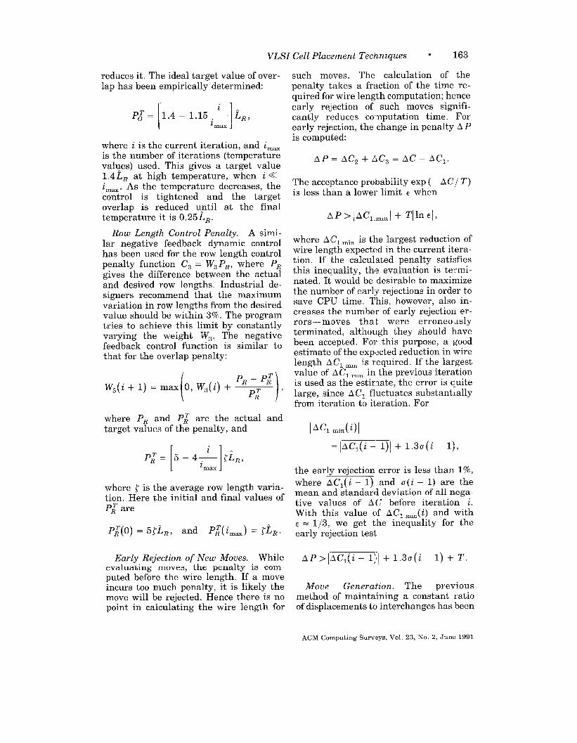
reduces it. The ideal target value of over-lap has been empirically determined:

[ “1P:= 1.4 – 1.15: LR,

i ~.X

where i is the current iteration, and i~ax

is the number of iterations (temperaturevalues) used. This gives a target value1.4 L~ at high temperature, when i <<

i ~ax. As the temperature decreases, thecontrol is tightened and the targetoverlap is reduced uanti 1 at the finaltemperature it is 0.25 L~.

Row Length Control Penalty. A simi-lar negative feedback dynamic controlhas been used for the row length controlpenalty function C3 = W3 P~, where PRgives the difference between the actualand desired row lengths. Industrial de-signers recommend that the maximumvariation in row lengths from the desiredvalue should be within 3!Z0. The programtries to achieve this limit by constantlyvarying the weight W~. The negativefeedback control function is similar tothat for the overlap penalty:

( PR – P;

i

W~(i+ 1) = max 0, Wa(i) + p~ ,R

where PR and P: are the actual andtarget values of the penalty, and

p; .

where 1 is thetion. Here theP: are

[ ‘15–4~ (LR ,i ~~,

average row length varia-initial and final values of

Early Rejection of New Moves. Whileevaluating mo~es, the penalty is com -puted before the wire length. If a moveincurs too much penalty, it is likely themove will be rejected. Hence there is nopoint in calculating the wire length for

such moves. The calculation of thepenalty takes a fraction of the time re-quired for wire length computation; hence

early rejection of such moves signifi-cantly reduces co reputation time. Forearly rejection, the change in penalty A Pis computed:

AP= ACZ +ACa = AC– ACI.

The acceptance probability exp ( - AC/T)is less than a lower limit ~ when

where A Cl ~,. is the largest reduction ofwire length expected in the current itera-tion. If the calculated penalty satisfiesthis inequality, the evaluation is termi-nated. It would be desirable to maximizethe number of early rejections in order tosave CPU time. This, however, also in-creases the number of early rejection er-rors—moves that were erroneouslyterminated, although they should havebeen accepted. For this purpose, a goodestimate of the expected reduction in wirelength ACI ~,. is required. If the largestvalue of A Cl ~,. in the previous iterationis used as the estimate, the error is quitelarge, since ACI fluctuates substantiallyfrom iteration to iteration. For

IAC1 ~,~(i)l

=lAC1(i - 1)1+ 1.3a(i - 1),

the early rejection error is less than 1%,

where ~Cl(i – 1) and u(i – 1) are themean and standard deviation of all nega-tive values of AC before iteration i.With this value of ACI ~,.(i) and with6 = 1/3, we get the inequality for theearly rejection test

AP>lACl(i– Ill + 1.3a(i– 1) + T.

Move Generation. The previousmethod of maintaining a constant ratioof displacements to interchanges has been


164 * K. Shahookar and P. Mazumder

discontinued. The following procedure isused for move generation.

A cell is selected randomly, and a ran-dom location is selected as the destina-tion. If the destination is vacant, adisplacement is performed; otherwisean interchange is performed. A newrange-limiting function has been used,which restricts the motion of a cell to itsneighborhood. This has caused a dra-matic improvement in the move accep-tance rate, thus saving the time beingwasted on evaluating moves that wouldbe rejected.

Temperature Profile. The tempera-ture profile is the key feature of thisalgorithm. The dramatic improvement inthe acceptance rate of new moves due tothe improved move generation functionhas made it unnecessary to start the al-gorithm at a very high temperature. Thetemperature profile used is

T1 = 500

T2+1= 0.98TC, l<i <120

(Compare with TimberWolf 3.2, whereT1 = 4,000,000.) Thus, about the samenumber of temperature steps are concen-trated in a smaller range. The finaltemperature is unchanged.

Acceptance Rate Control. Due to thewide variety of the circuits to be placed,a fixed temperature schedule does notalways produce an appropriate value ofthe rate of acceptance of new configura-tions. It was observed that the ideal ac-ceptance rate was 5070 in the beginning(i = O) and was reduced to zero at lowtemperatures (i = i~,x). To achieve thisaccept ante rate profile, negative feed-back control has been provided. The idealacceptance rate profile is given by

P: ( ‘).501–=i ~ax

This profile is achieved by scaling thechange in cost, AC:

AC’ = sAC,

where

where p, and p: are the actual and tar-get values of the percentage acceptancerate. This changes s by 2.5910 for l$ZOdeviation in p, and p:.

The algorithm was tested on six indus-trial circuits and was found to be 9-48times faster than TimberWolf 3,2, with aslightly better placement. It was alsotested on the MCNC benchmarks, andthe wire length obtained was 10-20%better than other algorithms. The timerequired to achieve this improvement,however, is not given.

Some other important contributions tocell placement by simulated annealingare Bannerjee and Jones [19861, Gidas

[19851, Greene and Supowit [1984],Grover [1987], Hajek [1988], Lam andDelosme [1988], Lundy and Mees [1984],Mallela and Grover [1988], Romeo andSangiovanni-Vincentelli [1985], Romeo etal. [1984], and White [1984].

2. FORCE-DIRECTED PLACEMENT

Force-directed placement algorithms arerich in variety and differ greatly inimplementation details [Hanan andKurtzberg [1972a]. The common denomi-nator in these algorithms is the methodof calculating the location where a mod-ule should be placed in order to achieveits ideal placement. This method is asfollows.

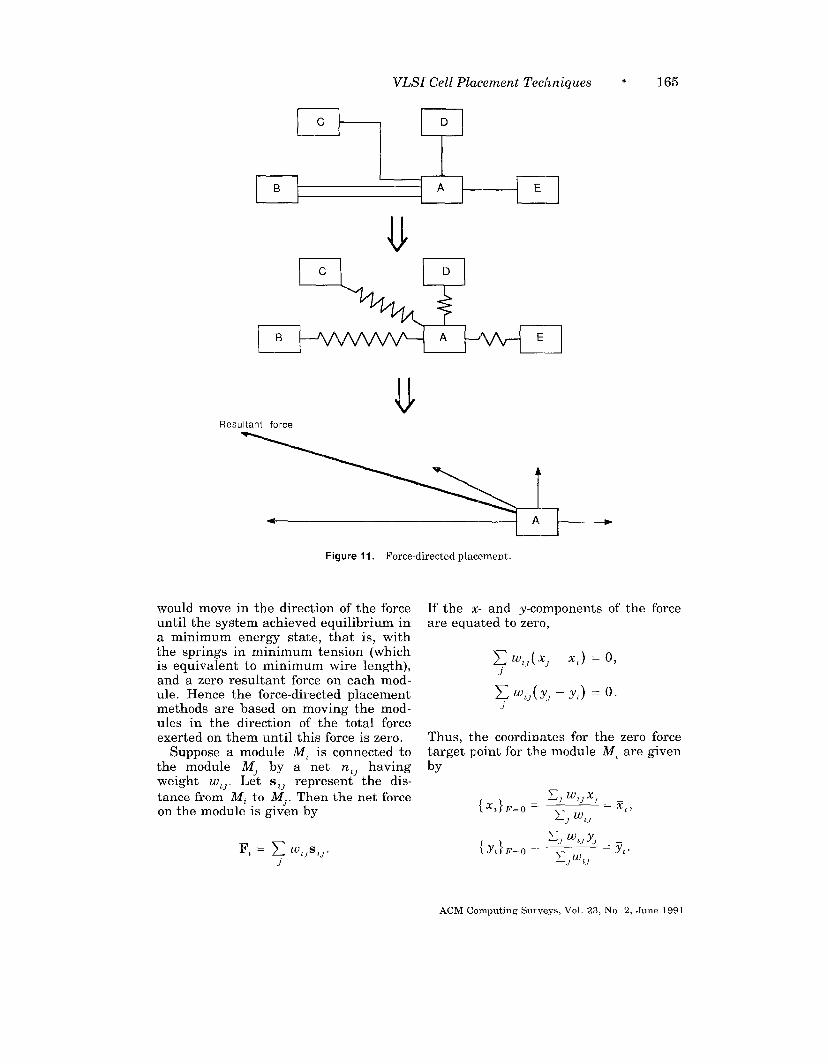
Consider any given initial placement.Assume the modules that are connectedby nets exert an attractive force on eachother (Figure 11). The magnitude of theforce between any two modules is di-rectly proportional to the distance be-tween the modules. as in Hooke’s law forthe force exerted by stretched springs,the constant of proportionality being thesum of weights of all nets directly con-necting them. If the modules in such asystem were allowed to move freely, they


VLSI Cell Placement Techniques * 165

‘T 7’El=

I 1

1A t---m

Resultant force

Figure 11. Force-directed placement.

would move in the direction of the forceuntil the system achieved equilibrium ina minimum energy state, that is, withthe springs in minimum tension (whichis equivalent to minimum wire length),and a zero resultant force on each mod-ule. Hence the force-directed placementmethods are based on moving the mod-ules in the direction of the total forceexerted on them until this force is zero.

Suppose a module M, is connected tothe module MJ by a net n,J havingweight w,]. Let s,~ represent the dis-

tance from M, to MJ. Then the net forceon the module is given by

J

If the x- and y-components of the forceare equated to zero,

x%,(x, - x,) = 0,

h(m) =o.J

Thus, tlhe coordinates for the zero forcetarget point for the module M, are givenby

ACM Computmg Sm veys, Vol. 23, No 2, June 1991


These equations resemble the center ofgravity equations; that is, if the modulesconnected to M, are assumed to be masseshaving weight w,,, then the zero force

target location of M, is the center ofgravity of these modules.

2.1 Force-Directed Placement Techniques

The early implementations of the force-directed placement algorithm were in the1960s [Fisk et al. 1967]. There are manyvariations in existence today. Some areconstructive; some are based on iterativeimprovement.

In constructive methods, no initialplacement exists; the coordinates of eachmodule are treated as variables, and thenet force exerted on each module by allother modules is equated to zero. By si-multaneously solving these equations, weget the coordinates of all modules. Insuch an implementation, care must betaken to avoid the trivial solution x, = x~and y, = y~ for all i, J“, which, consider-ing the spring model, obviously satisfiesthe zero force condition. Another prob-lem in this approach is that the zeroforce equations are nonlinear, becausethe force depends on distance, and theeuclidean distance metric involves asquare root; while the Manhattan dis-tance metric involves absolute values.Antreich et al. [1982] give an example ofthe equation-solving method.

In iterative methods, an initial solu-tion is generated either randomly or bysome other constructive method. Thenone module is selected at a time, its zeroforce target point is computed from theabove equations, and an attempt is madeto move the module to the target point orinterchange it with the module previ-ously occupying the target point. Suchalgorithms are also called force-directedrelaxation or force-directed pairwiserelaxation algorithms,

Here, one problem is to decide the or-der in which to select the modules formoving to the target location. In mostimplementations, the module or seedmodule with the strongest force vectoris selected. In other implementations,

the modules are selected randomly. Instill others, the modules are selectedon the basis of some estimate of theirconnectivity.

Another problem is where to move theselected module if the slot nearest to thezero force target location is already occu-pied, as it most probably will be. Onesolution is to move it to the nearestavailable free location. But the nearestfree location may be very far in somecases. This is an approximate methodand, at best, will need more iterations toachieve a good solution.

The second solution is to compute thetarget location of a module selected asdescribed above, then evaluate thechange in wire length or cost when themodule is interchanged with the moduleat the target location. If there is a reduc-tion in the wire length, the interchangeis accepted; otherwise it is rejected. It isnecessary to evaluate the wire lengthbecause it is possible that in an attemptto interchange the selected module withthe module previously at the target point,we are moving that other module faraway from its own target point; hencethe move can result in a loss instead of again.

The third solution is to perform a rip-ple move; that is, select the module pre-viously occupying the target point for thenext move. This process is continued un-til the target point of a module lies at anempty slot. Then a new seed is selected.

The fourth solution is to compute thetarget point of each module, then look forpairs of modules such that the targetpoint of one module is very close to thecurrent location of the other. If suchmodules are interchanged, both of themwill achieve their target locations withmutual benefit.

The fifth solution uses repeated trialinterchanges. If an interchange reducesthe cost, it is accepted; otherwise it isrejected. The cost function in this case isthe sum of the forces acting on the mod-ules. An example of the use of two typesof force functions for pairwise inter-change is given in Chyan and Breuer[1983].


VLSI Cell Placement Techniques 0 167

Hanan et al. [1976a, 1976b, 1978] dis-cuss and analyze seven placement algo-rithms, including three force-directedplacement techniques. Experimental re-sults are given in Hanan [1976a], and thealgorithms are discussed in Hanan[1976bl. Johannes et al. [19831, Quinn[19751, and Quinn and Breuer [1979]are implementations of the force-directedalgorithm.

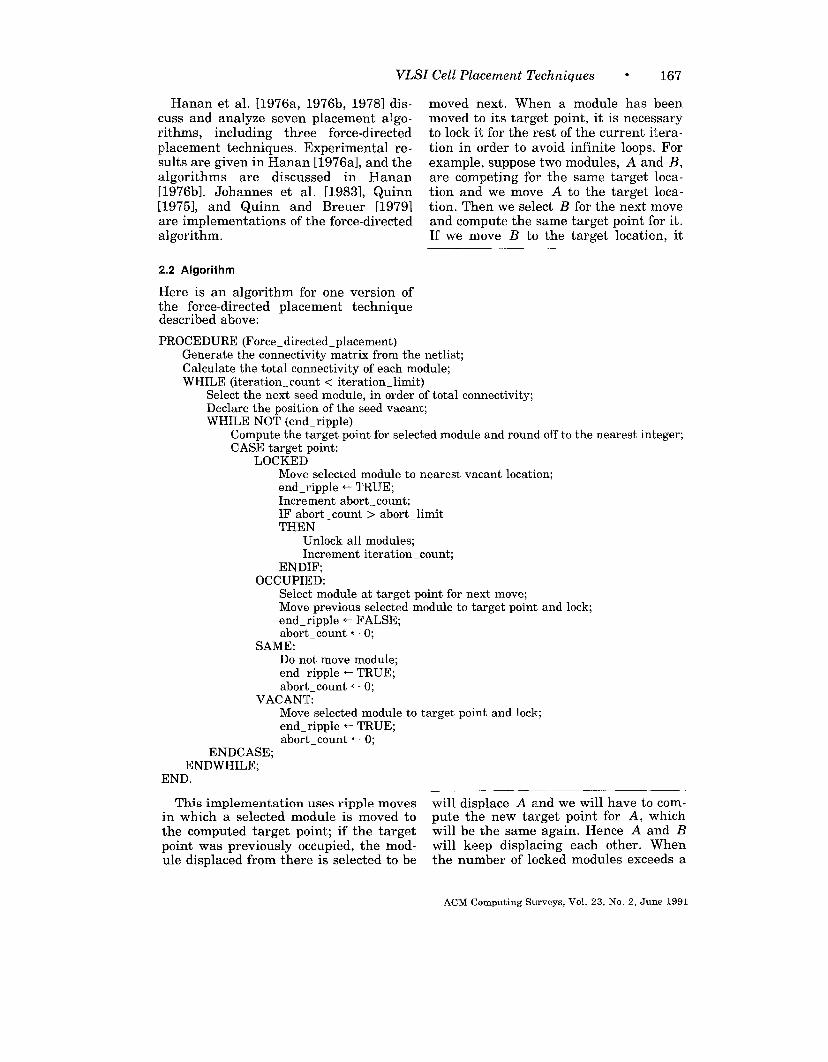
moved next. When a module has beenmoved to its target point, it is necessaryto lock it for the rest of the current itera-tion in order to avoid infinite loops. Forexample, suppose two modules, A and B,are competing for the same target loca-tion and we move A to the target loca-tion. Then we select B for the next moveand compute the same target point for it.If we move B to the target location, it

2.2 Algorithm

Here is an algorithm for one version ofthe force-directed placement techniquedescribed above:

PROCEDURE (Force _directed_placement)Generate the connectivity matrix from the netlist;Calculate the total connectivity of each module;WHILE (iteration_ count < iteration_ limit)

Select the next seed module, in order of total connectivity;Declare the position of the seed vacant;WHILE NOT (end_ ripple)

Compute the target point for selected module and round off to the nearest integer;CASE target point:

LOCKEDMove selected module to nearest vacant location;end_ripple + TRUE;Increment abort count;IF abort count > abort_ limitTHEN

Unlock all modules;Increment iteration _count;

ENDIF;OCCUPIED:

Select module at target point for next move;Move previous selected module to target point and lock;end.ripple + FALSE;abort_ count * O;

SAME:Do not move module;end_ripple + TRUE;abort _count + O;

VACANT:Move selected module to target point and lock;end_ripple + TRUE;abort _count + O;

ENDCASE;ENDWHILE;

END.

This implementation uses ripple moves will displace A and we will have to com-in which a selected module is moved to pute the new target point for A, whichthe computed target point; if the target will be the same again. Hence A and B

point was previously occupied, the mod- will keep displacing each other. Whenule displaced from there is selected to be the number of locked modules exceeds a



limit (depending on the size of thenetlist), there will be too many aborts.At that time all modules are unlockedagain, another seed is selected, and anew iteration is started.

2.3 Example

Consider a circuit consisting of nine mod-ules, with the following netlist:

netl= {13489}

net2= {156789}

net3= {245679}

net 4 = {3 7}

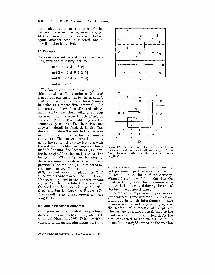
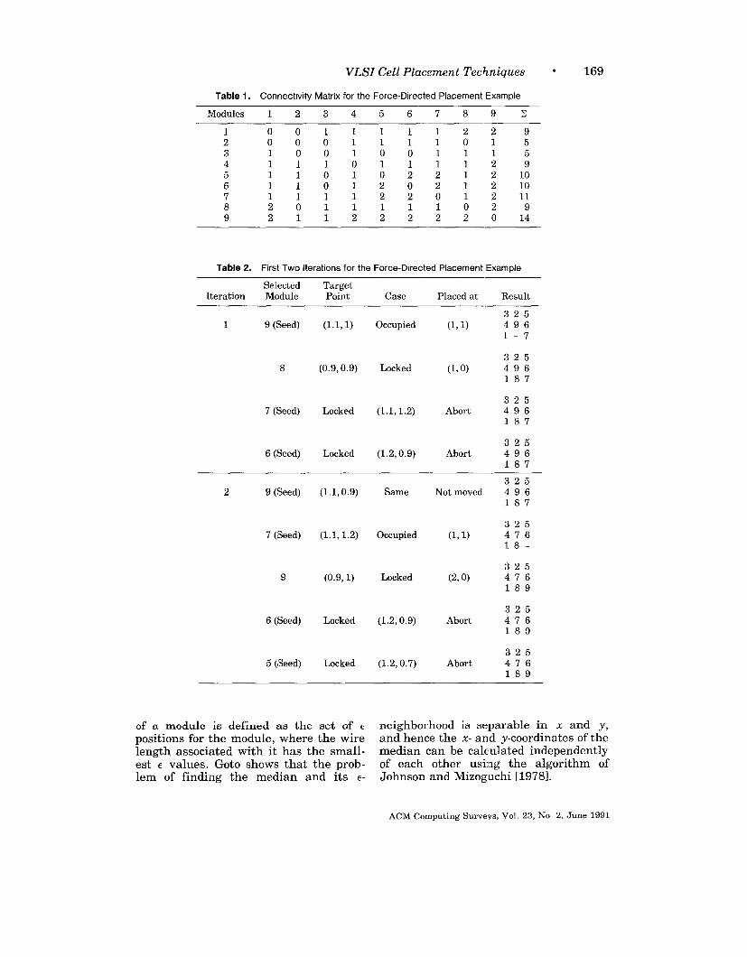
The lower bound on the wire length forthis example is 15, assuming each hop ofa net from one terminal to the next is 1unit (e. g., net 1 must be at least 4 unitsin order to connect five terminals). Todemonstrate how force-directed place-ment works, we start with a randomplacement with a wire length of 20, asshown in Figure 12a. Table I gives theconnectivity matrix. Two iterations areshown in detail in Table 2. In the firstiteration, module 9 is selected as the seedmodule, since it has the largest connec-tivity, 14. The target point is (1.1, 1),using the center of gravity formula withthe entries in Table 1 as weights. Hencemodule 9 is moved to location (1, 1), leav-ing its original location (O, 1) vacant. Thelast column of Table 2 gives the interme-diate placement. Module 8, which waspreviously located at (1, 1), is selected forthe next move. The target point is(0.9, 0.9), but we cannot place it at (1,1)since we already placed module 9 there.Hence, it is placed in the nearest vacantslot (0, 1). Then module 7 is selected asthe seed, and the process is repeated. Thefinal solution is shown in Figure 12b.The result is an improvement in wirelength of 3 units.

2.4 Goto’s Placement Algorithm

Goto proposed a somewhat unique force-directed placement algorithm [Goto 1981;Goto and Matsuda 1986]. This algorithmconsists of an initial placement part and

(a)

I 1

(b)

Figure 12. Force-directed placement example. (a)Random initial placement with wire length 20; (b)final placement after two iterations with wwelength 17.

an iterative improvement part. The ini-tial placement part selects modules forplacement on the basis of connectivity.When selected, a module is placed at thelocation that yields the minimum wirelength. It is not moved during the rest ofthe initial placement phase.

The iterative improvement part uses ageneralized force-directed relaxationtechnique in which interchanges of twoor more modules in the ~-neighborhood ofthe median of a module are explored.The median of a module is defined as theposition at which the wire length for thenets connected to the module is mini-mum. The e-neighborhood of the median

ACM Computing Surveys, Vol 23, No. 2, June 1991


Table 1. Connectwity Matrix for the Force-Directed Placement Example

e 169

Modules 1 2 3 4 5 6 7 8 9 X

12

34

5

678

9

0011111 22 90001111 01 51001001 11 51110111 12 91101022 12101101202 12101111220 12112011111 02 92112222 2014

Table 2. First Two Iterations for the Force-Directed Placement Example

Selected TargetIteration Module Point Case Placed at Result

---

1 9 (Seed) (1.1, 1) Occupied (1, 1)

8 (0.9, 0.9) Locked (1, o)

7 (Seed) Locked (1.1, 1.2) Abort

6 (Seed) Locked (1.2,0.9) Abort

2 9 (Seed) (1.1, 0.9) Same Not moved

7 (Seed) (1.1, 1.2) Occupied (1, 1)

9 (0.9, 1) Locked (2, o)



323496

1-7

325496187

325496187

325496187

325496

187

32547618-

325476189

325

476189

325

476189

of a module is defined as the set of c neighborhood is separable in x and y,positions for the module, where the wire and hence the x- and y-coordinates of thelength associated with it has the small- median can be calculated independentlyest e values. Goto shows that the prob - of each other using the algorithm oflem of finding the median and its e Johnson and Mizoguchi [19781.

ACM Computiug Surveys, Vol 23, No 2, June 1991


The ~-neighborhood of a given configu-ration in the configuration space is de-fined as the set of configurations that canbe obtained from the given configurationby circularly interchanging not morethan X modules. A configuration is saidto be h-optimal (locally optimal) if it isthe best one in such a neighborhood. Theprocess of replacing the current configu-ration with a better configuration fromits h-neighborhood is called local

transformation.The complete placement algorithm is

as follows. An initial placement is gener-ated. Generalized force-directed relax-ation is performed to obtain a h-optimumconfiguration. If the given amount ofcomputation time is not exhausted, thisprocedure is repeated with another ini-tial placement. The best result of all thetrials is accepted. The heuristic searchprocedure used for finding h-optimumconfigurations is now described.

The procedure consists of module inter-change cycles, iterated until there is nofurther improvement. At the beginningof each interchange cycle, a seed module(M) is selected and interchanged on atrial basis with all modules M(i) in its~-neighborhood (1 < i < ~). If there is areduction in wire length, the interchangeyielding the maximum reduction is ac-cepted, and the interchange cycle is ter-minated. If there is no reduction in wirelength, a triple interchange is tried be-tween the seed module M, a module M(i)in its c-neighborhood, and a module M( ij)in the c-neighborhood of M(i) (1 < i, j <e). This results in 62 trials in which themodules are interchanged in the cyclicorder M + M(i) -+ M(ij) + M. If there isa reduction in wire length, then the in-terchange giving the minimum wirelength is accepted, and the interchangecycle is terminated. Otherwise for each i,the j = j, giving the minimum wirelength is chosen for further processing.The next step is to try quadruple inter-changes between M, M(i), M( zj,) and themodules M( ij, k ) in the e-neighborhood ofM(~,) (1 < i, k < e). This once againresults in 62 interchanges of the formM+ M(i) ~ M(ij,) + M(ij, k) - M. Wechoose the k that results in the mini-

ACM Computmg Surveys, Vol. 23, No 2, June 1991

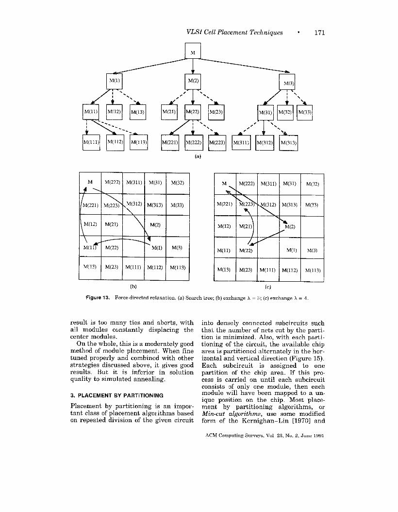
mum wire length for further processing.This process is repeated until inter-changes of i elements have been consid-ered. The possible interchanges areshown as a tree in Figure 13a. The inter-changes that result in the minimum wirelength at each step are represented bythe solid lines and are pursued further,whereas those represented by the dottedlines are abandoned. There is only onesolid line under any node, except the rootnode M.

The parameter ~ represents thebreadth of the search tree, and A repre-sents its depth. As e and A are increased,the h-optimal configuration gets better,but there is also a large increase in com-putation time. Goto observed that e =4-5 and h = 3-4 is the best compromisebetween placement quality and computa-tion time. These results were obtainedfrom experiments on a 151 module cir-cuit. For satisfactory placement of largercircuits, a higher value of ~ and h may benecessary.

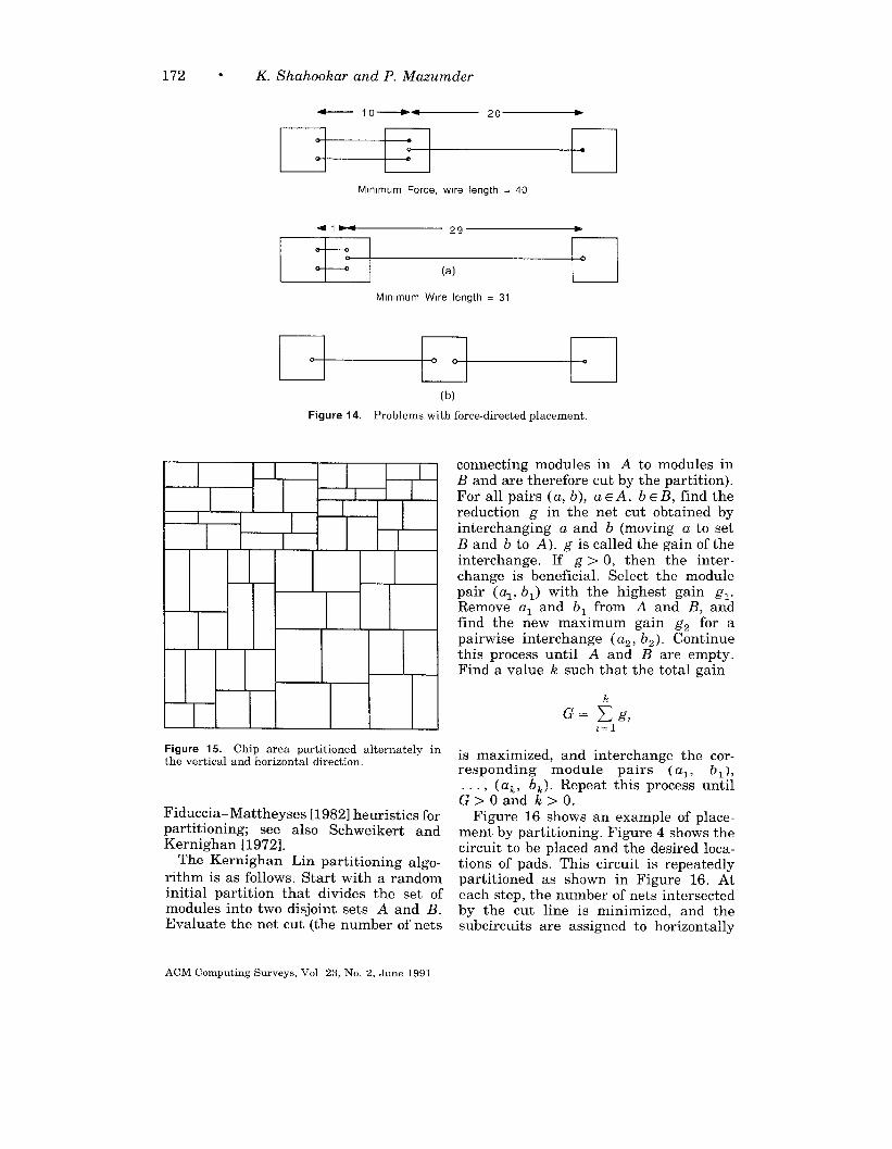
2.5 Analysis

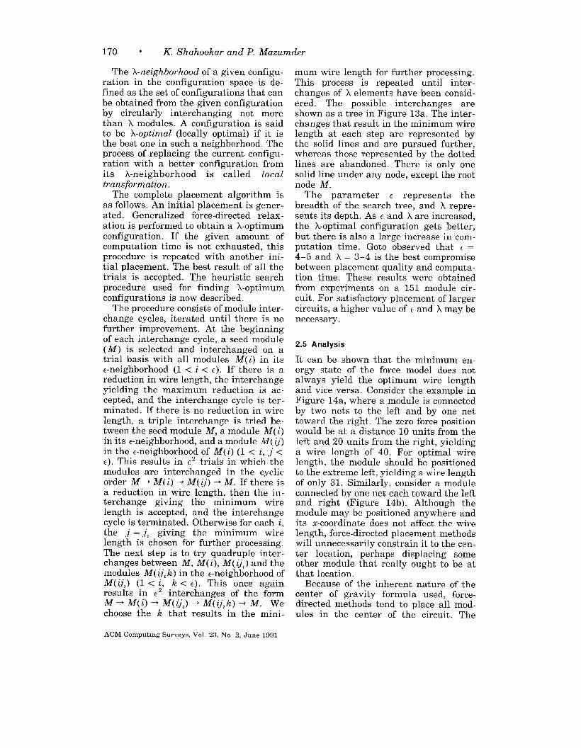
It can be shown that the minimum en-ergy state of the force model does notalways yield the optimum wire lengthand vice versa. Consider the example inFigure 14a, where a module is connectedby two nets to the left and by one nettoward the right. The zero force positionwould be at a distance 10 units from theleft and 20 units from the right, yieldinga wire length of 40. For optimal wirelength, the module should be positionedto the extreme left, yielding a wire lengthof only 31. Similarly, consider a moduleconnected by one net each toward the leftand right (Figure 14b). Although themodule may be positioned anywhere andits x-coordinate does not affect the wirelength, force-directed placement methodswill unnecessarily constrain it to the cen-

ter location, perhaps displacing someother module that really ought to be atthat location.

Because of the inherent nature of thecenter of gravity formula used, force-directed methods tend to place all mod-ules in the center of the circuit. The


nM

—————————mM(1) M(2)

,

“ f

M(3)

‘(”) ‘hub ti”iM!i13kl)AhE ‘::;‘FE‘(22’)f$!i’i d“ifl~”i

(a)

M M(222) M(311) M(31) M(32)

?~ ‘,

M(221) M(223) ,M(312) M(313) M(33)

M(12) M(21) M(2)

\\

M(l~/ ----% .~

M(22) %M(l) M(3)

M(13) M(23) M(lll) M(112) M(113)

(b)

M M(222) M(311) M(31) M(32)

xl \

\M(221) M(223 (312) M(313) M(33)

\

M(12) M(21) M(2)

/~ +Y

M(n) M(22) M(1) M(3)

M(13) M(23) M(lll) M(112) M(113)

(c)

Figure 13. Force-directed relaxation. (a) Search tree; (b) exchange h = 3; (c) exchange k = 4,

result is too many ties and aborts, with into densely connected subcircuits suchall modules constantly displacing thecenter modules.

On the whole, this is a moderately goodmethod of module placement. When finetuned properly and combined with otherstrategies discussed above, it gives goodresults. But it is inferl~or in solutionquality to simulated annealing.

3. PLACEMENT BY PARTITIONING

Placement by partitioning is an impor-tant class of placement algorithms basedon repeated division of the given circuit

that the nu”mber of nets cut by the parti-tion is minimized. Also, with each parti-tioning of the circuit, the available chiparea is partitioned alternately in the hor-izontal and vertical direction (Figure 15).Each subcircuit is assigned to onepartition of the chip area. If this pro-cess is carried on until each subcircuitconsists of only one module, then eachmodule will have been mapped to a un-ique position on the chip. Most place-ment by partitioning algorithms, orMin-cut algorithms, use some modifiedform of the Kernighan-Lin [1970] and


172 - K. Shahookar and P. Mazumder

Mln]mum Force, wire length = 40

*1~29 b

0- —0 0

& — (a)

Mlmmum Wire length = 31

0 ‘o 0 0

(b)

Figure 14. Problems with force-directed placement

11111--I I

I

I I I II

1 I II

II IFigure 15. Chip area partitioned alternately inthe vertical and horizontal direction,

Fiduccia-Matthey ses [1982] heuristics forpartitioning; see also Schweikert andKernighan [1972].

The Kernighan-Lin partitioning algo-

rithm is as follows. Start with a randominitial partition that divides the set ofmodules into two disjoint sets A and B.Evaluate the net cut (the number of nets

connecting modules in A to modules inB and are therefore cut by the partition).For all pairs (a, b), a cA, b e B, find thereduction g in the net cut obtained byinterchanging a and b (moving a to setB and b to A). g is called the gain of theinterchange. If g >0, then the inter-change is beneficial. Select the modulepair (al, bl) with the highest gain gl.Remove al and bl from A and B, andfind the new maximum gain gz for apairwise interchange ( az, bJ. Continuethis process until A and B are empty.Find a value k such that the total gain

G=~g,L=l

is maximized, and interchange the cor-responding module pairs (al, bl),

(a~, b~). Repeat this process untilG~Oandk>O.

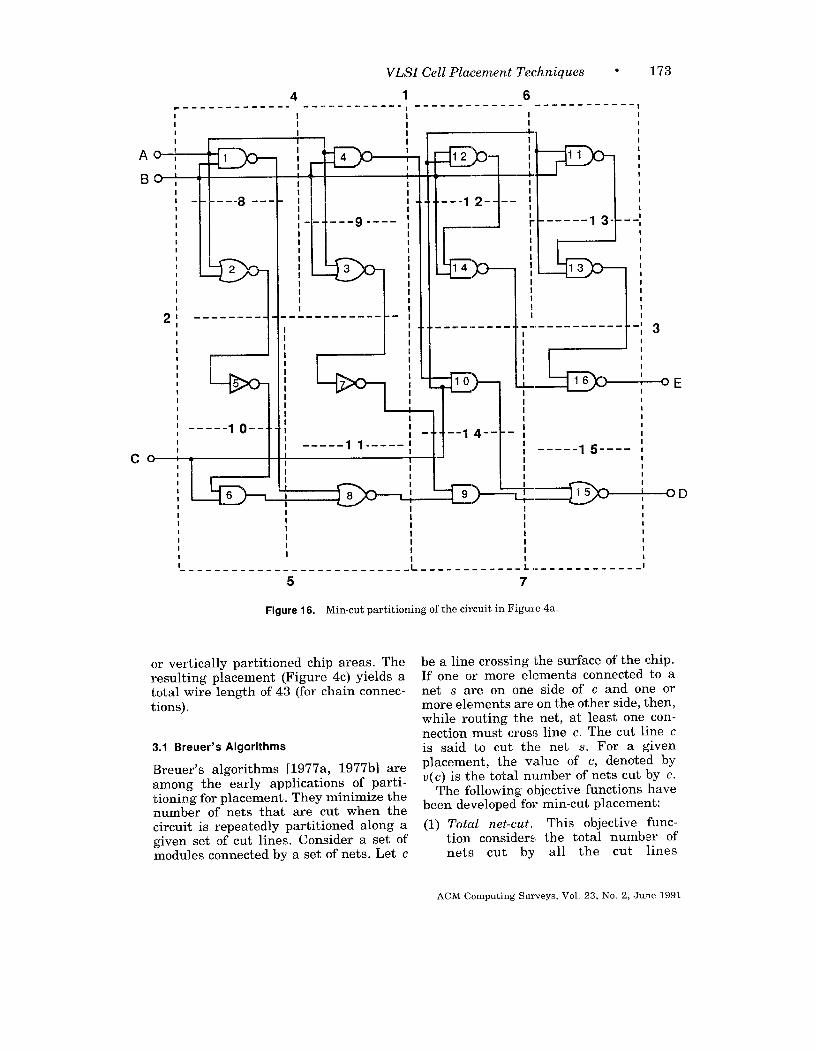
Figure 16 shows an example of place-ment by partitioning. Figure 4 shows thecircuit to be placed and the desired loca-tions of pads. This circuit is repeatedlypartitioned as shown in Figure 16. Ateach step, the number of nets intersectedby the cut line is minimized, and thesubcircuits are assigned to horizontally



4 1 6------ -- ----- ---- ----- ----, - ----- ----- ---- ----- ----- II I iI I I1

~1

1 1

TId 1

B:I

8I - --- ---I

[tI11 2

.4

:4--------.

II

II

I -- ---10 --

I

II

I

I 4II,I I1 II I1 iI

9I

I - -. ,------- 1I III[IIIII1

.----- ----- -

1

[

IIIIIIIII

-1III1I11

I I1

.~ !11 I

I1

I tII

II II tI II I

------- ---- --------------1I I

II

E

1II

I

I ‘ -11--14--1-! -----15----i-----1 1-----;

I11IIII----- -----

II iI !I II II I

I----- ----- ----- -- L-

5

Figure 16. Min-cut partitioning

or vertically partitioned chip areas. Theresulting placement (Figure 4c) yields atotal wire length of 43 (for chain connec-tions).

3.1 Breuer’s Algorithms

Breuer’s algorithms [1977a, 1977bl areamong the early applications of parti-tioning for placement. They minimize thenumber of nets that are cut when thecircuit is repeatedly partitioned along agiven set of cut lines. Consider a set ofmodules connected by a set of nets. Let c

iIIII

----- ----- - 1------

7

of the circuit in Figure 4a.

II1I1

t

------ --- I

be a line crossing the surface of the chip.If one or more elements connected to anet s are on one side of c and one ormore elements are on the other side, then,while routing the net, at least one con-nection must cross line c. The cut line cis said to cut the net s. For a givenplacement, the value of c, denoted byU(c) is the total number of nets cut by c.

The following objective functions havebeen developed for rein-cut placement:

(I) Total net-cut. This objective func-

tion considers the total number ofnets cut by all the cut lines



partitioning the chip,

N,(u) = ~u(c),

where the sum is over all verticaland horizontal cut lines. Consider acanonical set of cut lines as the col-lection of cut lines between each rowand each column of slots. Then, mini-mizing the total number of nets cutusing this set of cut lines is equiva-lent to minimizing the semiperimeterwire length. For a formal proof, seeBreuer [1977a, 1977bl.

(2) Min-max cut value objective function.In standard cell and gate array tech-nologies, the channel width, andtherefore the chip area, depend onthe maximum number of nets beingrouted through a channel at any pointor the maximum net-cut for any cutline across the channel. The form ofthis objective function is

NC(mM) = ~ maxv(c),channels CCC,

where CL is a set of cut lines definedacross channel i. Note that for thisobjective function, only the net-cut inthe congested region of the routingchannel is significant, and the algo-rithm will try to minimize this maxi-mum net-cut, even at the expense ofincreasing the net-cut in other vacantregions of the channel.

(3) Sequential cut line objective function.Although the above objective func-tions better represent the placementproblem, it is computationally diffi-cult to minimize them. A third objec-tive function is therefore introduced,which is easy to minimize but doesnot give a globally optimal place-ment. As the name implies, the objec-tive is to make one cut and minimizethe net-cut, then to cut each groupagain and minimize the net-cut withrespect to these cut lines and subjectto the constraints already imposed bythe previous cut, and so on. Note thatbecause of the sequential (greedy) na-ture of this objective function, it does

not guarantee that the total numberof nets cut by all cut lines will beminimized. Hence, minimizing thisobjective function is not equivalent tominimizing the semiperimeter wirelength.

3. 1.1 Algorithms

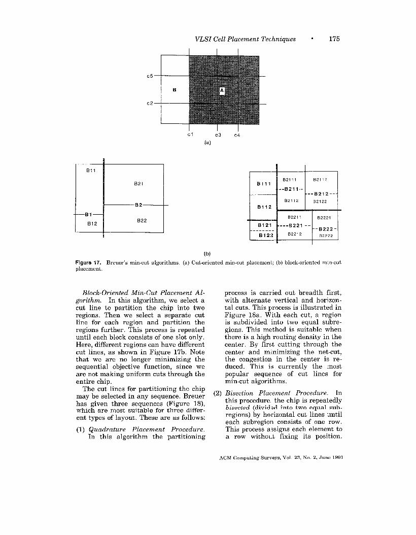
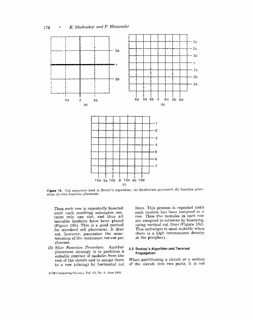
Breuer has explored two basic placementalgorithms. Each of these algorithms re-quires a given sequence of cut lines thatpartition the chip, so that each sectioncontains only one slot. To be consistentwith Breuer’s notation, in the followingdiscussion the subsections of the chip cre-ated by the partitioning process are calledblocks. These should not be confused withmacro blocks.

Cut Oriented Min-Cut Placement Algo-rithm. Start with the entire chip and agiven set of cut lines. Let the first cutline partition the chip into two blocks.Also partition the circuit into two subcir -cuits such that the net-cut is minimized.Now partition all the blocks intersectedby the second cut line, and partition thecircuit correspondingly. Repeat this pro-cedure for all cut lines. This process isshown in Figure 17a.

This algorithm realizes the sequentialobjective function described above. Inpractice, however, this algorithm does notalways give good results because of twoproblems associated with it. ConsiderFigure 17a. While processing cut line C2,we must partition blocks A and B cre-ated by c1 simultaneously. First, if thereis a way to partition them sequentially,computation time would be saved as aresult of a reduction in the problem size.Besides, a conflict can arise when we tryto bisect blocks A and B using the samecut line. lf the modules of A to be placedabove C2 require a larger area than thecorresponding elements in B, then it isimpossible to bisect A and B with thesame cut line, and a less optimal parti-tion has to be accepted. To avoid both ofthese problems, another algorithm is pre-sented in which each block is partitionedusing a separate cut line.

ACM Computmg Surveys, Vol 23, No. 2, June 1991


C5

C2

c1 C3 C4

(a)

Bll

B21

B2—

—B1

B12B22

- 1

EmB2111 B2112

Bill--B211 -

-- B212--

B2112 B2122B112

B221 1 B2221

Figure 17. Breuer’s rein-cut algorithms.placement.

(b)

(a) Cut-oriented rein-cut placemen~; (b) block-oriented rein-cut

Block-Oriented Min-Cut Placement Al-gorithm. In this algorithm, we select acut line to partition the chip into tworegions. Then we select a separate cutline for each region and partition theregions further. !l%is process is repeateduntil each block consists of one slot only.Here, different regions cam have differentcut lines, as shown in Figure 17b. PJotethat we are no longer minimizing thesequential objective ftmction, since weare not making uniform cuts through theentire chip.

The cut lines for partitioning the chipmay be selected in any sequence. 13reuerhas given three sequences (Figure 18),which are most suitable for three differ-ent types of layout. These are as follows:

(1) Quadrature Placement Procedure.In this algorithm the partitioning

(2)

process is carried out breadth first,with alternate vertical and horizon-tal cuts. This process is illustrated inFigure 18a. With each cut, a regionis subdivided into two equal subre -gions. This method is suitable whenthere is a high routing density in thecenter. E3y first cutting through thecenter and minimizing the net-cut,the congestion in the center is re-duced. This is currently the mostpopular sequence of cut lines forrein-cut algorithms.

Bisection Placement Procedure. Inthis procedure, the chip is repeatedlybisected (divided into two equal sub-regions) by horizontal cut lines untileach subregion consists of one row.This process assigns each element toa row withotk fixing its position.



Figure

4a 2 4b

(a)

18. Cut sequences

3a

2a

3b

1

3C

2b

3d

6a 5a 6b 4 6C 5b 6d

(b)

1

2

3

4

5

6

7

10a 9a10b 8 10c 9b 10d

(c)

used in Breuer’s algorithms. (a) Quadrature placement;

ment; (c) slice/bisection placement.

Then each row is repeatedly bisecteduntil each resulting subregion con-tains only one slot, and thus allmovable modules have been placed(Figure 18b). This is a good methodfor standard cell placement. It doesnot, however, guarantee the mini-mization of the maximum net-cut perchannel.

(3) Slice Bisection Procedure. Anotherplacement strategy is to partition asuitable number of modules from therest of the circuit and to assign themto a row (slicing) by horizontal cut


(b) bisection place-

lines. This process is repeated untileach module has been assigned to arow. Then the modules in each roware assigned to columns by bisecting,using vertical cut lines (Figure 18c).This technique is most suitable whenthere is a high interconnect densityat the periphery.

3.2 Dunlop’s Algorithm and Terminal

Propagation

When partitioning a circuit or a sectionof the circuit into two parts, it is not


(a)

(b)

A

x

c

(c) (d)

Figure 19. Terminal propagation. 0, real module; 0, dummy module.

sufficient to consider only the internalnets of the circuit, which may intersectthe cut line. Nets connecting externalterminals or other modules in anotherpartition (at a higher level) must also beconsidered. Dunlop and Kernighan [19851do this by a method called terminal prop-agation. Figure 19 illustrates the needfor terminal propagation. Figure 19ashows the First division of the entire cir-cuit into two sections. If a module isconnected to an external terminal on theright side of the chip, it should be prefer-entially assigned to the right side of thechip, and vice versa. If this constraint

was not considerecl, then each half of thecircuit could have been assigned to eitherside of the chip. Figure 19b shows theresult after several levels of partitioning.A particular net has cells connected to itin sections A, B, and C as shown. Whenthese sections are partitioned further, itwould be preferable to place these cellsin the bottom half of A but in the tophalf of ~. The assignment in B does notaffect the wire length. Dunlop andKernighan [1985] implement terminalpropagation as follows.

Consider the situation when A is be-ing partitioned vertically and the net



connecting cells 1, 2, and 3 in A alsoconnects other cells in B and C. Suchcells in other partitions are assumed tobe at the center of their partition areas(points X and Y in Figure 19c) and arereplaced by dummy cells at the nearestpoints on the boundary of A (e. g., atX’, Y’). Now, during partitioning, thenet-cut would be minimized if the cells 1,2, and 3 are placed in the bottom half ofA. A similar process for B does not yieldany preference (Figure 19d), as predictedabove.

To do terminal propagation, the parti-tioning has to be done breadth first.There is no point in partitioning onegroup to finer and finer levels withoutpartitioning the other groups, since inthat case no information would be avail-able about which group a module shouldpreferentially be assigned to.

The algorithm is in production use aspart of an automated design system. Thealgorithm has been tested on a chip with412 cells and 453 nets. It yields areaswithin 10–20% and track densitieswithin 3% of careful hand layouts. CPUtime of the order of 1 h on a VAX 11/780has been reported. The CPU time can besignificantly improved using theFiduccia-Mattheyses [1982] linear-timepartitioning heuristics.

3.3. Quadrisection

Suaris and Kedem [1987] have suggestedthe use of quadrisection instead of bipar -titioning to divide the chip vertically andhorizontally in a single partitioning step(Figure 20a), resulting in a truly two-di-mensional placement procedure, ratherthan adapting a basically one-dimen-sional partitioning procedure to solve thetwo-dimensional placement problem. Thequadrisection algorithm used is an ex-tension of the Kernighan-Lin [1970] andFiduccia-Matthey ses [1982] heuristics.

Unlike the Kernighan-Lin algorithmdescribed above, a module in one quad-rant can be interchanged with modulesin any of the other three quadrants. Thisgives 12 gain tables, each correspondingto a pair of quadrants. At each step, the

pairwise interchange giving the highestgain is selected.

The cost function is computed as fol-lows. Let the cells connected to net n andplaced in quadrant K be denoted bya~( n). Then the cell-distribution vectorfor the net n is

a(n) = (al(n), az(n), a~(n), aq(n)).

Associated with each net is a residentflag vector,

~(n) = (~l(n), ~,(n), ~,(n), ~,(n)),

such that

PK(n) ={

1 ifa~(n) >0

0 otherwise.

Thus, the Kth component of B(n) indi-cates whether any cells connected to netn are in quadrant K.

The cost function is defined as

W= ~~N~n(B(n)),

where w.( /3(n)) is the cost of net n. If twoor more components of /3(n) are nonzero,then there are cells connected to that netin the corresponding quadrants, and thenet is being cut. The weights w~ and w,,are associated with horizontal and verti-cal net-cuts, respectively. The relativevalues of these weights indicate the pref-erence in wiring direction. According toSuaris and Kedem [1987], in double- andtriple-metal technology, where almost theentire space over the cells can be used forwiring, we would prefer vertical (overthe cell) wiring. This would conservechannel space, which would otherwise beneeded for horizontal wiring spans.Hence, in such technologies, Wu is usu-ally set much less than w~.

If all modules connected to a net are inhorizontally adjacent quadrants, then thecost w.( P( n)) = wk. Similarly, if they arein vertically adjacent quadrants, thenw.( (3(n)) = Wu. If the modules are in di-agonally opposite quadrants or if theyare distributed over any three quadrants,then w~(/3( n)) = Wh + WU. If the rnodu]esconnected to a net n are distributed over



B ?2 621

B*

’23 B 24

B3 z 631

—-r-——+,—jE1332 ~

LB 342 ~ B341

6331

-----A -----,34

---”B33----

~333 : 63346343 : B344

CHIP

—B1—

B1:3 % 4

B42 f341

_B4 ;I

!-t :

B’432 / 0431 442: B441

----B44--

------ %5------

0433 / B434E1443 ~B444

&B14m-!---lf---f+-=+FL11

+ :l:;B:+q:ltB4;+T;r, ,

’331 ‘3: KB333B334B341 ‘342 B343B344B431 E432B433B434 B441E442B443F444

Figure 20a. Quadrisection.

all four quadrants, there are two possibleinterconnection patterns— one with onehorizontal and two vertical cuts and theother with one vertical and two horizon-tal cuts. If WU< w~ as described above,we choose the first pattern and w.( (3(n))=2WU+ w~.

If the cost function w~(~( n)) is suchthat it can be computed from 6(n) inlinear time, it can be proved that the

quadrisection algorithm also runs in lin-ear time. The rest of the partitioningalgorithm is the same as in Fiduccia andMattheyses [1982] and Kernighan andLin [1970].

The terminal propagation method in-troduced by Dunlop and Kernighan [1985]has bee n extended for quadrisection asshown in Figure 20b. The figure showsregions 5 and 6 about to be partitioned


180 . K. Shahookar and P. Mazumder

‘1 2 5 ,,11t,11#1

3 4 L----------- ,------

B~0

D1

A x 1,I

61 7I11I D1 c1--- .--1---,111,I11

Figure 20b. Terminal propagation in quadrisection.

along the dotted lines and cells 1? and ~in these regions connected to cells A andC in other regions. In this example, it

would be beneficial to assign ~ to thelower left quadrant of region 5, as shown,and l) to the upper or lower right quad-rant of region 6 (since the exact positionof C has not been determined yet). Ter-minal propagation is done by insertingtwo kinds of dummy cells—fixed and par-tially fixed at appropriate locations.Thus, in region 5, the influence of A isrepresented by a dummy cell X fixed inthe lower left quadrant. The dummy cellwill bias 1? into the same quadrant inorder to reduce net-cut. In region 6, thecell c is represented by a partially fixeddummy cell Y, which is restricted to theupper and lower right quadrants. Thiswill bias D into one of these quadrants.

Global routing information is also usedto improve the efficiency of terminalpropagation. For example, in Figure 20b,cells connected to the same net are lo-cated in all four quadrants and are to beconnected as shown. Here, A and Bshould influence each other’s positionthrough terminal propagation, and soshould B and C’. Since there is no directconnection between A and C, however,there is no need for propagating them.After each partitioning step, the cells in

different quadrants are connected in apattern that gives the minimum cost, asdiscussed above. As the partitioning pro-ceeds, these connection patterns give aglobal routing tree for each net. In theterminal propagation phase, only thosemodules that are directly connected toeach other are propagated. The arrowsshow the effect of terminal propagation.For example, cell C will be biased to-ward the upper left quadrant when re -gion 7 is quadrisectioned.

The algorithm has been implementedas part of the VPNR place and routepackage. Preliminary experiments showthat this algorithm compares favorablywith TimberWolf 3.2. For various stan-dard cell circuits, this algorithm yieldedan area within + 5~o of the area yieldedby TimberWolf. This algorithm, how-ever, achieved this layout quality 50-200times faster than TimberWolf. Run timesreported are of the order of 1.4 min for a304-cell circuit and 1 h for a 2907-cellcircuit on a VAX 8600.

3.4 Other Techniques

Many variations of the rein-cut place-ment algorithm have been suggested.Lauther [19791 applies this method forthe placement of macro cells and uses



repeated partitioning to generate mutu-ally dual placement graphs. His imple -mentation also includes an improvementphase in which module rotation, mirror-ing, and other compression techniquesare used.

corrigan [19791 has developed anotherimplementation of placement based onpartitioning. Wipfler et al. [19821 dis-cusses a combined force and cut algo-rithm for placement. Shiraishi andHerose [1980] have developed a rein-cutbased algorithm for master slice layout.

3.5. Analysis

The strength of rein-cut algorithms isthat they partition the problem intosemi-independent subproblems. The con-cept of minimum net-cut implies a mini-mum amount of interaction between theparts that are placed independently. Di-viding the problem into small partsbrings about a drastic reduction in thefactorial search space.

Partitioning can be thought of as asuccessive approximation method forplacement. At each level of partitioning,the modules are localized in the region ofthe chip in which they ought to be finallylocated, but their exact position is notfixed. As the circuit is further parti-tioned and the smaller groups of modulesare assigned to smaller chip areas, weget a better approximation of their finalcoordinates. This algorithm is less sus-ceptible to local minima because the co-ordinates of all modlules are beingapproximated simultaneously, withmutual benefit.

The problem with this technique is thatpartitioning is itself an NP completeproblem and, therefore, is computation-ally intensive. This method is used forplacement because heuristics developedso far for partitioning are much better interms of speed and performance thanthose for placement. Note, however, thatobtaining an optimal partitioning doesnot guarantee an optimal placement, al-though it would be close.

Overall, the results obtained fromplacement by partitioning algorithms are

second only to simulated annealing. Be-side, these algorithms take much lessCPU time.

4. NUMERICAL OPTIMIZATION TECHNIQUES

Grouped together in this section are somecomputationally intensive deterministictechniques based on equation solving andeigenvalue calculations or on numericaloptimization, such as the Simplexmethod. So far these techniques havemainly been used for macro blocks. Themain problem encountered in using thesetechniques is that the placement problemis nonlinear. Two different approachesare used to overcome this obstacle. Onemethod is to approximate the problem bya linear problem, then use linear pro-gramming. The other method is to usethe various nonlinear programmingmethods [Walsh 19751. Examples of bothmethods are give n in the following sec-tions.

4.1 Eigenvalue Method

Quadratic Assignment Problem[Gilmore 1962]. Given a cost matrix CZJrepresenting the connection cost of ele -ments i and J and a distance matrix dk 1representing the distance between loca-tions k and 1, find a permutation func-tion, p, that maps elements i, j, . . . tolocations k = p(i), 1 = p(j), . . . such thatthe sum

@ = x f% dP(2)P(J)L,J

is minimized. Consider the placementproblem, where c,~ is the connectivitybetween cell i and cell j and dkl is thedistance between slot k and slot 1. Thepermutation funcbion p maps each cell toa slot. The wire length is given by theproduct of the connectivity and the dis-tance between the slots to which the cellshave been mapped. Thus, @ gives thetotal wire length for the circuit, which isto be minimized. Hall [19701 has formu-lated the cell placement problem as aquadratic assignment problem and de-vised a novel method to solve it by usingeigenvalues.


182 - K. Shahookar and P. Mazumder

Let C be the connection matrix. Let c,be the sum of all elements in the ith rowof C. Define a diagonal matrix D suchthat

dZJ ={

o, i # J“,c ~> i =J”.

The matrix 1? is defined as

B= D–C.

Further, let XT = [xl, XZ, . . . . x.] and

YT=[yl, y2, ..., y.] be row vectors rep-

resenting the x- and y-coordinates of thedesired solution. Then it can be proved[Hall 19701 that

@( X,Y) = X~BX+ Y~BY.

Thus the problem is reduced to minimiz-ing *(X, Y) subject to the quadraticconstraints

XTX= 1 and YTY=l.

These constraints are required to avoidthe trivial solution x, = O for all i. Theminimization is done by introducingthe Lagrange Multipliers a and b andforming the lagrangian

L = XTBX+ YTBY

— Q!(x~x- l)-o(Y~Y -1).

Equating the first partial derivatives ofL with respect to X and Y to zero, weget

2BX–2a X=0 2BY–2~Y=0

or

(B-cYI)X=O (B-(31 )Y=0.

These equations yield a nontrivial solu-tion if and only if a and 6 are eigenval-ues of the matrix B and X and Y arethe corresponding eigenvectors. Premul -tiplying these equations by XT and Y ~,respectively, and imposing the con-straints X ‘X = 1 and Y T Y = 1, we get

@( X,Y) = XTBX+ YTBY= a +6.

Thus, in order to minimize the value ofthe objective function @, we must choosethe smallest eigenvalues as a solution

for a and (3. The corresponding eigen-vectors X and Y will give the x- andy-coordinates of all the modules. If O = Al< Az < Aa < “ “ “ < Am are the distincteigenvalues of B, then taking a = 6 = Alwill give the minimum value @ = O, xlwill be proportional to y,, all x, will beequal, and all y, will be equal. If it isdesired that X not be proportional to Y(i.e., we require a two-dimensional solu-tion with all modules not placed along astraight line), we must select differenteigenvalues for a and (3. Further, if it isdesired that not all x, or all Y, be equal,we should ignore Al = O. Thus, a nearoptimal nontrivial solution is a = Az, 6= As. The components of the eigenvectorassociated with the second-smallesteigenvalue give the x-coordinates of allthe modules, and the components of the

eigenvector associated with the third-smallest eigenvalue give the y-coordi-nates of all modules.

4.1.1 Example

An example is given in Figure 21. Thenetlist for the problem is

IVl = {1,3}; Nz= {1,4}; N~= {2,4};

NL= {2,3}; N~= {2,3},

The C, D, and B matrixes are

[1

0011~=oo21

12001100

r20001

r20 -1-11

B= _~ 3 ‘2 ‘1–2 3 0

1-1 -1 0 2j

The eigenvalues of B are O, 2, 2.586,and 5.414. The eigenvectors correspon-ding to the eigenvalues 2 and 2.586 are

[1 -1 -1 11 and [1 -0.414 0.414 -1](Table 3). These eigenvectors give the x-and y-coordinates, respectively, for allfour modules.

ACM Computmg Surveys, Vol. 23, No, 2, June 1991

VLSI Cell Placement Techniques o 183

1

3 4

(a)

4

1 *1

3*

, I e-1

1

2*

-1 *4

(b)

5(3’12 ~-l 4 7

! I I

(c)

Figure 21. Placement by the eigenvalue method:An example. (a) Example circuit; (b) placement inthe euclidean plane determined by the eigenvec-tore; (c) assignment to regularly spaced slots.

Table 3. Eigenvectors of Matrix B, Givingthe Solution in Euclidean Space

Module x-Coordinates y-Coordinates

1 12 –1 – :.4143 –1 0.4144 1 –1

Eigenvalues 2 2.586

4. 1.2 Analysis

This is an 0( n2) algorithm. A weaknessof the algorithm is that it does not takemodule size, shape, and routing channelwidth into account. It assumes that themodules are zero-area points. Therefore,it does not correspond very well to themodule placement problem, where themodules must be placed at grid points orin rows. After this algorithm has deter-mined the placement that minimizes thetotal wire length, mapping the modulesform this placement to grid points can bevery difficult for large circuits, with manyties requiring arbitrary decisions. Thewire length is often increased signifi-cantly while converting the result of thisalgorithm to a legal placement.

4.2 Resistive Network Optimization

Cheng and Kuh [19841 have devised anovel technique folc placement. They havetransformed the placement problem intothe problem of minimizing the power dis-sipation in a resistive network. The ob-jective function (squared euclidean wirelength) is written in matrix form, whichyields a representation similar to thematrix representation of resistive net-works. The placement problem is solvedby manipulating the corresponding net-work to minimize power dissipation us-ing sparse matrix techniques.

4.2.1 Objective Function and Analogy to

Resistive Networks

The wire length is taken as the square ofthe euclidean distance between con-nected modules:

@(x, Y)

—— : f,+,- X,)2+(yL-yJ)’],

where c,~ is the connectivity betweenmodules i and j. This can be written as

@( X,Y) = XTBX+ Y~BY,

where B = D – C as defined in theeigenvalue method described in Sec-tion 4.1. If this equation is compared to



Tabla 4. Analogy Between the Placement Problem and Power Dissipationm a Resistwe Network

Resistive network Placement problem

Power, P Wire length, @Nodes ModulesActive voltage sources, U2 Fixed module coordinates, X2Passive node voltages, UI Movable module coordinates, xlAdmittance, Y Connectivity, B

the equation for power dissipation in aresistive network,

P= vTYnv,

we find that B is of the same form as theindefinite admittance matrix Y. of ann-terminal linear passive resistive net-work. The coordinate x, is analogous tothe voltage at node i. The connectivityc is analogous to the mutual conduc -t~nce between nodes i and j, and d,, isanalogous to the self-admittance at nodei. If the given netlist contains some fixedmodules, such as pads located at the chipboundary, then that will be equivalent tohaving a fixed voltage at the correspond-ing nodes in the resistive network. Thus,fixed modules are equivalent to voltagesources. This analogy is summarized inTable 4, In a resistive network (Fig-ure 22), the current always distributesitself so as to minimize the power dissipation. Hence the problem reduces tosolving the network equations for cur-rent. This current will then give the opti-mal power dissipation and hence optimalplacement. If there are no pads or otherfixed modules, that case would be analo-gous to a passive resistive network withno voltage sources. All currents would bezero, which would yield a placement withall modules placed at the center of thechip. Hence fixed modules, preferably atthe periphery, are required to spread theother modules out. Even then, modulesare mostly clustered near the center. Thisalgorithm uses scaling and relaxation asdescribed below to spread them out overthe entire chip.

4.2.2 Slot Constraints

Slot constraints are required to guaran-tee module placement at grid points orlegal values. A permutation vector p is


1

2

m

m+l

~ Linear passive ~+~

resistive

network

=(a)

—m+l

Linear passiveresistive m+2

n

W+++———

v

(b)

Figure 22. Cell placement by resistive networkoptimization. (a) n-terminal linear resistive net-work with m terminals floating and n-m terminalsconnected to voltage sources; (b) resistive networkwith linear constraints.

defined such that the ith component p,is the ith legal value or slot available fora module to occupy:

P= [Plj P2, . . .. Pm]T.

Let the position vector be

ul=[xl,.x2,..., xm]T.


The placement problem then consists ofmapping each module to one slot; that is,associating each x, with a pj. The fol-lowing slot constraints are necessary toyield a legal solution:

,$1xi = ,$,p,m m

i=l ~=1

. m

The proof is given in Cheng and Kuh

[19841. As a simple example, consider afour module placement problem, withfour given slot coordinates, pl, . . . . Pb.Then the assignment

xl=p~; x2=p4;

X3 =p~; X4= pl

is a legal placement. It is easy to see thatall the above constraints are satisfied. Iftwo modules overlap, however,

the above constraints will not be satis-fied. Using all of the above constraints inthe optimization process is not easy com-mutationally. If we use only the first fewconstraints, we will get a solution thatsatisfies the corresponding properties, butthe modules will not be located at theexact slot locations. For example, the firstconstraint helps align the center of grav-ity of the modules with that of the slots.Hence, using only this constraint willcause the resulting placement to becentered in the chip area.

4.2.3 Procedure

The overview of the placement procedureis as follows. First, the given circuit ismapped to a resistive network, where thefixed modules and pads are representedas fixed voltage sources. The power dissi -

pation in the network is minimized, us-ing only the first slot constraint. Thiscauses al 1 the modules to cluster aroundthe center of the chip. The next step isscaling, in which the second slot con-straint ia used to spread the modules.Then repeated partitioning and relax-ation are ~erformed. This rn-ocess alignsthe

(1)

(2)

modul~s with the slot lhcations. -

Optimization. The power dissipa-tion in the network is optimized us-ing t:he linear slot constraint. Theoptimization is done by applying theKuhn-Tucker formula,

u, = Y;/[-Y12U2+ i,],

where

The goal of the optimization methodis to reduce the euclidean wire length;that goal is best achieved by cluster-ing all the modules close to eachother. The use of the first constraintonly centers the module placement inthe chip area. If there are no fixedcoordinates around the periphery ofthe chip, the optimization step willyield a trivial solution with all mod-ules located at the center. With somemodules at the periphery, a mini-mum wire length solution like theone shown in Figure 23a is obtained(for the netlist of Figure 4a).

Scaling. In order to spread out themodules, the higher order slot con-straints are required. In the secondstep, Cheng and Kuh [1984] repeatthe optimization procedure using thesecond (parabo lie) constraint. Thiswill increase the power dissipationcompared to the optimal but imprac-tical solution of the previous step.The objective now is to find a config-uration that results in a minimumincrease in power dissipation. Usingthis objective, ~heng and Kuh [19841



(a)

(b)

(c)

Figure 23. The partitioning step in resistive net-work optimization.

have derived the following equations,which give module coordinates thatare more spread out:

x01

— cox T2L= a. + c~,

a.

where XO, denote the solution afteroptimization, x~z denote the new so-

(3)

(4)

lution after scaling,

[

1/2

an= + ,~1 ( PL - c.)’1

co= ; :1XOL

L

[ 1

1/2

ao= ;-,(%-co)’ .L

Relaxation. In this part of the algo-rithm, optimization and scaling arerepeatedly done on subregions of size(3 specified by the user. First, opti-mization and scaling are done on oneend region of size ~, then on the otherend region, and finally on the middleregion. While doing optimization andscaling on one subregion, the rest ofthe modules are assumed to be fixed.By this process, the module positionsare iteratively fine tuned.

Partitioning and assignment. Afterthe above steps, the modules are stillnot located exactly at the given slotlocations. The next step is iterativepartitioning into smaller and smallerregions. At each step, optimizationand seal ing are performed on thesubregions according to the aboveequations. Every time, the linear slotconstraint aligns the center of grav-ity of the group of modules with thecenter of the region in which it isbeing placed. At the last level of par-titioning, when each section consistsof only one module, the module isaligned to the center of the slot. Thisprocess is illustrated in Figures 23band c.

4.2.4 Complexity and Results

Since linear network computations arerequired and sparse matrix techniquesare used, the computation complexity is0( ml 4)log2 m, where m is the numberof movable modules.



The algorithm has been tested on the34 module example given by Steinberg[1.9611, and Hall [19701 and its perfor-mance compared against Steinberg’sassignment algorithm and Hall’seigenvalue method. The wire length was10% less compared to the eigenvaluemethod and 30% less compared to theSteinberg algorithm. A run time of 13.1s was reported on a VAX 11/780. Theperformance was also compared to thealgorithms of Stevens [1972] and Quinnand Breuer [19791 for a 136 module prob-lem. The improvement m wire lengthwas 9.5% over Stevens and 21 YO overQuinn and Breuer, and the CPU timeWaS 104.2 S.

4.3 PROUD: Placement by Block Gauss-Seidel

Optimization

Tsay et al. [19881 recently proposed animproved algorithm based on the resis-tive network analogy. The method con-sists of repeated solution of sparse linearequations. The slot constraints describedabove are bypassed, and the partitioningscheme is simplified. Block Gauss-Seidel(BGS) iteration is used to resolve theplacement interactions between theblocks, The algorithm proceeds in twophases. First, global placement is doneby the Successive Over RelaxationMethod (SOR). This results in an optimalsolution. The modules, however, are con-sidered as zero-area points and are notconfined to the grid points, Then, moduleshape and area are taken into considera-tion, and the chip is partitioned alter-nately in the vertical and horizontaldirection. At each step BGS iteration isperformed on each subregion in order toremove module overlap and successivelyapproximate the module positions withthe grid points. This process is repeateduntil each subregion consists of only onemodule.

4.3.1 Global Placement

First, the equations given in Section 4.4.2are solved using SOR, which is a gener-alization of the BGS method. The method

is as follows. To solve the equation

Axl = b,

A= A(L+I+ U),

where A is a diagonal positive definitematrix and L and U are lower and uppertriangular matrices, respectively. Thevector x ~ is solved iteratively by therecursive formula

Xl(k + 1) = Mxl(k) + a,

where

M = (I+ ZUL)-l[(l - w) I - UJU]

and

a = ZU(I+ wL)-l A-lb.

The parameter w is in the range O to 2.With w = 1, the SC)R method is reducedto the BGS method.

This method gives the global optimumsolution because, in the absence of slotconstraints, the objective function (theeuclidean wire length) is convex and hasa unique global minimum, which canbe determined by solving the matrixequations.

4.3,2 Partitioning and /3GS Iteration

The object of the partitioning and BGSiteration step is to ensure that for eachsubregion the total area of the modulesplaced on one side of the center line isequal to the total area of the modulesplaced on the other side of the centerline. The partitioning is done as follows.Each cut is placed so that the total areaof the modules on either side of the cut(as given by the global placement) isequal. If the cut line coincides with thecenter of the layout area, then the parti-tion process is continued to the next hier-archy level; otherwise, the followingmethod is used to align the cut with thecenter of the subregion.

Let the cut be to the right of the cen-ter. Then all modules to the right of thecenter line are projected to the centerline, only those modules that lie betweenthe cut line and the center line are con-sidered as movable, and the global place-ment phase is repeated in the left half



plane. Then the modules in the left halfplane are projected on the center line asfixed modules, and the global placementproblem is solved for the right half plane.This procedure will align the cut linewith the center line of the subregion be-ing divided. The partitioning is repeatedalternately in the horizontal and verticaldirections until each subregion containsonly one module.

In order to explain the intuitive con-cepts behind this method, Tsay et al.[19881 gave an analogy with rein-cut al-gorithms. This algorithm can be consid-ered as a form of rein-cut algorithm,which uses quadratic assignment insteadof the Kernighan–Lin heuristics for par-titioning. An optimal placement resultsin a rein-cut partition at any cut linethrough it. Thus, we can repeatedly de-termine the optimum but irregularplacement of point modules in the eu-clidean plane by solving the quadraticassignment problem and subdivide theplane to get a rein-cut partition. If thisprocess is repeated until each partitionconsists of only one module, we get anear-optimal placement with no over-laps, and the modules constrained to gridlocations, just like in the rein-cut algo-rithm. The quadratic assignment prob-lem can be solved using powerful sparsematrix techniques.

4.3.3 Complexity and Results

The algorithm has been implemented inthe Proud-2 placement system. It wastested on nine circuits consisting of1000-26,000-modules. In all cases, theresults were superior to those of Timber-Wolf 3.2 and comparable to those ofTimberWolf 4.2. The time required toachieve these results was about 50 timesless compared to TimberWolf 4.2. Forexample, a 26,000-module circuit re -quired a run time of about 50 min on aVAX 8650. For a 1438 module example,Proud-2 required 50 s, TimberWolf 3.2required 7200 s, and TimberWolf 4.2 re-quired 3260 s. Compared to the wirelength achieved by Proud-2, the resultsof TimberWolf 3.2 were 7. l% worse, and

the results of TimberWolf 4.2 were 9.6%better.

4.4 ATLAS: Technique for Layout Using

Analytic Shapes

Sha and Blank [19871 (and earlier Shaand Dutton [19851) used the PenaltyFunction Method (PFM), a nonlinear nu-merical optimization method, for blockplacement. They devised a modified ob-

jective function for macroblocks, whichallows computationally efficient rotationand mirroring. They also made an excel-lent comparison between simulated an-nealing and numerical techniques.

4.4.1 Objective Function

The objective function used to estimatethe wire length is the same as that de-scribed in Sha and Dutton [19851, withmodifications to accommodate block rota-tion and mirroring. The original objec-tive function is as follows:

Let Sk be a net connected to mk blocks,with centers at Cl(xl, Y1), . . ., C2(X2,

Yz), ...> C~~ Xn,, y~,) and the center of

gravity of the net Sk be Gk ( ~h, ~h),where

The squared wire length of the net Sk(Figure 24a) is defined as

If m, is the total number of nets, theobjective function is defined as

m’.

w= E-wk

= ,:1,:1{(~t - %)2+ (Yz- z)’}.

In macro placement, block orientationis important besides block position be-cause of two reasons. In order to fit theirregularly shaped blocks together whileminimizing the wasted space, all possible


(x,,


Module pln

/ /,

A

— Net center of gravity

(a)

.

(X’p, y~)(Xp, yp)

,-----%;----- ‘--- -------------------:

:I ‘.

‘.IIt ‘. Iu ‘. 1I h! ‘“J3

‘.& (X12, Y17) \Y ;-----------~----:’il

------ ------ ------. ---+

(X f,yj)

‘:----+- 1’

. 189

Ih,

?

(b)‘w’

Figure 24. Squared euclidean wire length function, Wk = AG2 + BG2 + CC,2 + DG2; (b) pin positionafter rotation in Atlas.

orientations should be allowed. Besides,rotation and mirroring have a significanteffect on the wire length. If the pins onone side (left, say) of a large block areconnected to other blocks placed on theother side (right), then the nets are forcedto go around the block. Flipping the blockover reduces the wire length.

Block Rotation. If a block is rotatedthrough an angle 6’, the pin coordinates

( ~~, y:) relative to the block center aregiven by

x; = XPCOS6 –yPsin6,

y~=yPcos O+xPsin O,

where x and yP are the original coordi -f“nates re atlve to the block center (Fig-

ure 24b). Let the block axis be defined bythe pair of coordinates ( X,l, y,l) and

( $,Z, Y,z) and the block center be denoted



by (+, Y,). Let

AY, =IY,l– Y,217

d, = ~-

Xpal=—,

d,

Yp()+—.

d,

Then, we get the absolute pin positionafter rotation:

x jJL = XL + alAx, – azliy,,

The new parameters introduced in theobjective function are constants XPand yp. Since no new variables areintroduced, there is little increase incomputation time.

Mirroring. The mirroring operation isrealized by introducing an extra vari -able, u,, such that u, = 1 means normalorientation and u, = – 1 means mirroredorientation. The pin position is now givenby

x pL = x, + alAxZ – Uzcy2fiyL,

These pin coordinates are used along withthe block coordinates in order to calcu-late the wire length more accurately.During optimization, u, is treated as acontinuous variable that can vary with-in the bounds I UZI = 1. A constraint

(u, – l)(uZ + 1) = O is imposed duringthe optimization process. This constraintmakes u converge to either + 1 or – 1.

4.4.2 Constraint Conditions

In addition to the above objective func-tion, some constraints are imposed dur-ing the solution process in order toensure a legal placement. Theseconstraints are only summarized here.For a detailed discussion, see Sha andDutton [1985].

Let the block width be w, and the blockheight be h,, with 1, = w, – h,, and Ax,,A y,, and d, be as defined above. Theconstraint that prevents block overlap isgiven by

gl(i,~) = r,+ r~ – d(i, ~) = 0;

r,, rJ are the block radii (half the blockheight), and d( i, j) is the distance be-tween the axes of the blocks i and j. Forthe derivation, see Sha and Dutton[19851.

Only two block orientations, verticaland horizontal, are allowed. To ensurethis, the orientation constraint is used:

gz(i) = Ax, Ay, /lt=O

for i=l,2, . . ..m.

It is obvious that if the block is not verti-cal or horizontal, both Ax, and A y, willbe nonzero, and the constraint will not besatisfied.

The constraint for the desired blocksize is given by

gs(i) = Z,– d, =0.

Let the desired chip aspect ratio be q,with the vertical and horizontal dimen-sions y~ and x~ = qyn, respectively.Then, the boundary constraints are

g41z(i) = r, – Xtz~O,

g42z(i) = r, – YLz~O,

g43~(i) = x,z + r, – .r~=o,

g..l(i) = Y,, + T-c- ym~o,

forl=l,2; i=l,2, . . ..m.

4.4.3 Penalty Function Method

The penalty function method consists ofthe following procedure:

(1) Select an increasing series Ck,

typically

co = 1; Ck+l = lock.



(b)

(a)

(c)

nD

Figure 25. PFM optimization process: Intermediate results as Cfi is increased.

(a) Construct a new unconstrained objec- and a solution is obtained. Fimre 25ative function P( x, c~) such that -

P( x, y, Ch) = objective function

+ Ck~ constraints.

(3) Use an unconstrained optimizationtechnique such as Newton’s methodto minimize P( x, y, c~) for k =0,1,2,. ... until the coordinates ofthe modules satisfy the constraintswithin the required accuracy.

Thus, in PFM during the first itera-tion, the constraints are reemphasized

shows the result of the first iteration,with c~ = 1. Then, in each iteration theweight of the constraints is increased andthe objective function minimized. Thiscauses the constraints to be satisfied moreand more accurately, at the expense ofan increase in the value of the objectivefunction. An intermediate result is shownin Figure 25b. As c~ is increased, themodules attain the proper orientation andoverlap is reduced. The process is termi-nated when the ccmstraints are satisfiedwithin the desired accuracy. Figure 25cshows the final result, with all modules



in either vertical or horizontal orienta-tion and no overlap.

4.4.4 Comparison with Simulated Annealing

PFM uses numerical techniques, whereassimulated annealing uses a statisticalapproach. Although the techniques ofnonlinear programming and simulatedannealing are very different, some simi -larities exist. The parameter c~ in PFMbehaves like the reciprocal of tempera-ture (1/ 7’) in simulated annealing. Insimulated annealing, moves are ran-domly generated, whereas in PFM movesare deterministic and are in the directionthat minimizes the penalty functionP( x, y, c~). The important feature of PFMis that all blocks move simultaneously,not one at a time as in simulated anneal-ing.

PFM has been tested on two chips with23 and 33 macro cells, and the resultshave been compared to those of Timber-Wolf and industrial placement. A 50%improvement over industrial placementand 23% improvement over TimberWolfwere reported. The CPU time reported isof the order of 2 h on a VAX station II fora 33-block circuit.

4.5 Algorithm for Block Placement by SizeOptimization

One example of linearization is providedby Mogaki et al. [19871. They presentedan algorithm for the placement of macroblocks to minimize chip area under con-straints on block size, relative block posi-tion, and the width of the availableinterlock routing space. This algorithmiteratively determines the optimum blocksize and relative block placement in or-der to reduce the wasted space and mini-mize the total chip area. Channel widthsare also considered during the optimiza-tion process. This is a quadratic integerprogramming problem, which has beenreformulated as a linear programmingproblem and solved by the Simplexmethod. This algorithm is the extensionof the work of Kozawa et al. [1984], anduses their Combined and Top Down

Placement (CTOP) algorithm for the ac-tual block placement. This is coupledwith block resizing by linear program-ming. This algorithm is suitable onlywhere block sizes are not yet fixed andmacro blocks can be generated with arange of possible aspect ratios. Hence,choosing the block aspect ratios to fittogether nicely in the placement, thengenerating the macro blocks results in acompact layout.

The first step is to generate an initialplacement by the CTOP algorithm. Thisalgorithm works by repeatedly combin-ing two blocks to form a hyper-blockuntil the entire chip consists of onehyper-block. At each step, blocks arepaired so as to minimize the wasted spaceand maximize their connectivity to eachother. Repeated combining of blocks gen-erates a combine tree with the entirechip as the root node and the individualblocks as leaves. This tree is then tra-versed top down, such that for each hy -per-block, a good placement is deter-mined for its component blocks. Thisgives the relative placement of the blocks.

The relative placement is converted toa Block Neighboring Graph (BNG), asshown in Figure 26. Each block is repre-sented as a node in the BNG, and eachsegment of a routing channel betweentwo blocks is represented by an edge con-necting the nodes. Formally,

BNG = G(V, E)

such that

V= {u} U{ L, R, B, T};

EC VXVX{X, Y} X{6},

where u represents a block, L, R, B, Tare the simulated blocks correspondingto left, right, top, and bottom edges of thechip, X or Y represent whether thechannel is vertical or horizontal, and 8 >0 represents the minimum channelwidth.

The next step is the linear program-ming formulation for block size optimi-zation. This consists of the objectivefunction and the constraints.


VLSI Cell Placement Techniques . 193

7-k

Y.

u F1En Elt–– ‘“ --+j~uvyx“ xv

Figure 26. Example macro-block layout and its block neighboring graph. ❑ , Block; o, simulated block;+ , vertical edge; ---> , horizontal edge.

4.5.1 Objective Function aspect ratio. Let the minimum and maxi-mum desirable values of the chip aspect

The primary objective is to minimize the ratio be ~.chip area. Wire length is considered indi -

and r+:

rectly through its effect on the chip area. YThere is a user-specified limit on the chip

r–~ — <r+.x



4.25

3.25

2.25

1.25

0

:::::: :::

25 0.35 0.45 0.55 0.65

x

Figure 27. Linear programming: objective function,

If r- and r+ are sufficiently close, weget

r=~=-.x

The chip area is given by

Ar[rx+ y)’.A=xy=~

Since the function (rx + y)2 increasesmonotonically with ( rx + y) for x, y > 0,the chip area function can be replaced byrx + y, which is a linear function, be-cause r is a constant. Thus, in orderto minimize chip area xy, the linearprogramming problem is formulated tominimize rx + y. The effect of this lin-earization is shown in Figure 27. Theshaded region represents the allowedvalues of chip width and height. Thisregion is bounded by the maximum andminimum chip area constraints and themaximum and minimum aspect ratioconstraints. Within a small aspect ratiorange, the linearized area is a good ap-proximation to the actual area.


4.5.2 Constraints

(1) Block size constraint. Each blockhas a given range of candidate sizesgiven by (wU(i), h“(i)), where i =1,2,. ... Nu. Nu is the number of pos-sible sizes for block u. The object ofthe linear programming approach isto choose the aspect ratio that resultsin the minimum wastage of chip area.Let AU(i) be the selection weight forthe ith candidate block size such that

~ Au(i) = 1, O<hU(i)S1.1=1

Au(i) represents the probability dis-tribution for selection of each candi-date block size. The expected blockwidth and height are therefore givenas

w. = 5 Au(i) wlu(i)&=l

hu = ~ AU(i) hU(i).L=l

These are the block size constraints.


(2) Channel width constraints. ILetXU, yU, x., yu be the coordinates ofblocks u and U, respectively, and WUand h ~ be the width and height ofblock u. If block u is to the right ofblock u, with a channel of width 6UUbetween them, we have

$“– (Xu+r.uu) ~~.u

for each edge

(u,u>x,~uu)=~,

as shown in Figure 26. Similarly, ifblock u is below block U, we get thecorresponding constraint

Y“– (Yu + Wu) =6.”

for each edge

(u, u, Y,8Uu]e E.

These constraints make it possible todetermine an appropriate blocksize when the channel widths arespecified.

Thus, the objective of the linear pro-gramming formulation is to determineXU, yU, WU, hU for all blocks u so that thelinearized area r-x + y is minimized, sub-ject to the above constraints.

4.5.3 Procedure

The algorithm can be summarized asfollows:

(1)

(2)

Determine the relative block place-ment by the CTCDP algorithm[Kozawa et al. 1984].

Determine the absolute block place-ment by the following repetitiveprocedure:

(2.1)

(2.2)

Determine the channel width byglobal routing.

Optimize block size using thefollowing optimization algo -rithm:

(2.2.1)

(2.2.2)

Generate the BNG fromthe relative block posi-tions.

Eliminate redundantconstraints and convertthe rest into an LP con-dition matrix.

(2.2.3) Solve the LP problem bythe Simplex method.

(2.2 .4) Select the block size

closest to the LP scdu-tion.

(2.3) (]0 to 2.1

The algorithm has been tested on twochips with up to 40 macro blocks. Experi-mental results indicate that 690 saving ofarea can result over manual designs and5-10% over other algorithms. This sav-ing is achieved, however, at the cost of10-12 times the computation time com-pared to other algorithms.

4.6 Other \(Vork in This Field

Blanks [1985a, 1985b] has exploited themathematical properties of the quadratic(sum of squares) distance metric to de-velop an extremely fast wire length eval -uation scheme. He uses the eigenvaluemethod to determine the lower bound onthe wire I ength in order to evaluate hisiterative improvement procedures. Hehas also given a theoretical model toexplain the observed deviation fromoptimality.

Markov et al. [1984] have usedBender’s [1962] procedure for optimiza-tion. Blanks [1984] and Jarmon [1987]have used the least-squares technique.Akers [1981] has used linear assignment.He has given two versions-constructiveplacement and iterative improvement.Further work on the eigenvalue methodhas been done by Hanan and Kurtzberg

[1972bl. Hillner et al. [19861 has pro-posed a dynamic programming approachfor gate array p Iacement (see alsoKarger and Malek [19841). Herrigel andFichtner 11989] have used the PenaltyFunction Method for macro placement.Kappen and de Bent [1990] have pre-sented an improvement over Tsay et al.’salgorithm discussed in Section 4.3.

5. PLACEMENT BY THE GENETIC

ALGORITHM

The genetic algorithm is a very powerfuloptimization algorithm, which works byemulating the natural process of evolu-tion as a means of progressing toward


196 * K. Shahookar and P. Mazumder

the optimum. Historically, it precededsimulated annealing [Holland 1975], butit has only recently been widely appliedfor solving problems in diverse fields, in-cluding VLSI placement [Grefenstette1985, 1987]. The algorithm starts withan initial set of random configurations,called the population. Each individual inthe population is a string of symbols,usually a binary bit string representinga solution to the optimization problem.During each iteration, called a genera-tion, the individuals in the current popu-lation are eualuated using some measureof fitness. Based on this fitness value,individuals are selected from the popula-tion two at a time as parents. The fitterindividuals have a higher probability ofbeing selected. A number of genetic oper-ators is applied to the parents to gener-ate new individuals, called offspring, bycombining the features of both parents.The three genetic operators commonlyused are crossover, mutation, and inver-sion, which are derived by analogy fromthe biological process of evolution. Theseoperators are described in detail below.The offspring are next evaluated, anda new generation is formed by sel-ecting some of the parents and off-spring, once again on the basis oftheir fitness, so as to keep thepopulation size constant.

This section explains why genetic algo-rithms are so successful in complex opti-mization problems in terms of schemataand the effect of genetic operators onthem. Informally, the symbols used inthe solution strings are known as genes.

They are the basic building blocks of asolution and represent the properties thatmake one solution different from theother. For example, in the cell placementproblem, the ordered triples consisting ofthe cells and their assigned coordinatescan be considered genes. A solutionstring, which is made up of genes, iscalled a chromosome. A schema is a setof genes that make up a partial solution.An example would be a subplacement,consisting of any number of such triples,with ‘don’t cares’ for the rest of the cells.A schema with m defining elements and

‘don’t cares’ in the rest of the n – mpositions (such as an m-cell subplace -ment in an n-cell placement problem)can be considered as an (n – m)-dimensional hyperplane in the solutionspace. All points on that hyperplane (i. e.,all configurations that contain the givensubplacement) are instances of theschema. Note here that the subplace -ment does not have to be physically con-tiguous, such as a rectangular patch ofthe chip area. For example, a good sub-placement can consist of two densely con-nected cells in neighboring locations.Similarly, a good subplacement can alsoconsist of a cell at the input end of thenetwork and a cell at the output end thatare currently placed at opposite ends ofthe chip. Both of these subplacementswill contribute to the high performance ofthe individual that inherits them. Thus,a schema is a logical rather than physi -cal grouping of cell-coordinate triples thathave a particular relative placement.

As mentioned above, the genetic opera-tors create a new generation of configu-rations by combining the schemata (orsubplacements) of parents selected fromthe current generation. Due to thestochastic selection process, the fitterparents, which are expected to containsome good subplacements, are likely toproduce more offspring, and the badparents, which contain some bad sub-placements, are likely to produce less off-spring. Thus, in the next generation, thenumber of good subplacements (or high-fitness schemata) tends to increase, andthe number of bad subplacements (low-fitness schemata) tends to decrease. Thus,the fitness of the entire population im-proves. This is the basic mechanism ofoptimization by the genetic algorithm.

Each individual in the population is aninstance of 2‘ schemata, where n is thelength of each individual string. (This isequivalent to saying that an n-cell place-ment contains 2” subplacements of anysize. ) Thus, there is a very large numberof schemata represented in a relativelysmall population. By trying out one newoffspring, we get a rough estimate of thefitness of all of its schemata or subplace -



FB:!:~J Cug1,1,,1,,

Chromosomal Rep. Physical Layout

Figure 28. Traditional method of crossover. A segment of cells is taken from each parent. The coordinatearray is taken from the first parent. With this method, cells B and F are repeated, and cells H and I areleft out.

ments. Thus, with each new configura-tion examined, the number of each of its2 n schemata present in the population isadjusted according to its fitness. This ef-fect is termed the intrinsic parallelism ofthe genetic algorithm. As more configu-rations are tried out, the relative propor-tions of the various schemata in the pop-ulation reflect their fitness more andmore accurately. When a fitter schema isintroduced in the population through oneoffspring, it is inherited by others in thesucceeding generation; therefore its pro-portion in the population increases. Itstarts driving out the less fit schemata,and the average fitness of the populationkeeps improving.

The genetic operators and their signifi-cance can now be explained.

Crossover. Crossover is the main ge-netic operator. It operates on two in-dividuals at a time and generates anoffspring by combining schemata fromboth parents. A simple way to achievecrossover would be to choose a randomcut point and generate the offspring bycombining the segment of one parent tothe left of the cut point with the segmentof the other parent to the right of the cutpoint. This method works well with thebit string representation. Figure 28 gives

an example of crossover. In some applica-tions, where the symbols in the solutionstring cannot be repeated, this method isnot applicable without modification.Placement is a typical problem domainwhere such conflicts can occur. For ex-ample, as shown in Figure 28, cells Band F are repeated, and cells H and Iare left out. Thus, we need either a newcrossover operator that works well forthese problem domains or a method toresolve such conflicts without causingsignificant degradation in the efficiencyof the search process. The performance ofthe genetic algorithm depends to a greatextent on the performance of thecrossover operator used. Variouscrossover operators that overcome theseproblems are described in the followingsections.

When the algorithm has been runningfor some time, the individuals in the pop-ulation are expected to be moderatelygood. Thus, when the schemata from twosuch individuals come together, the re -suiting offspring can be even better, inwhich case they are accepted into thepopulation. Besides, the fitter parentshave a hligher probability of generatingoffspring. This process allows the algo-rithm to examine more configurations ina region of greater average fitness so the



4 +CELL ABC DE FGHIJ

x 020507590030507095Y 00 00 05050505050

SERIALNO O , 23456709

J1CELL AFCDEBGI+I,J

x 020507590030557095Y 10 0 0 0 0 50 505050W umhan.ti

SERIALNO0 1 2 3456789 J

Chromosomal Rep.

Figure 29.

optimum may be determined and, at thesame time, examine a few configurationsin other regions of the configuration spaceso other areas of high average perfor-mance may be discovered.

The amount of crossover is controlledby the crossover rate, which is defined asthe ratio of the number of offspring pro-duced in each generation to the popula-tion size. The crossover rate determinesthe ratio of the number of searches inregions of high average fitness to thenumber of searches in other regions. Ahigher crossover rate allows explorationof more of the solution space and reducesthe chances of settling for a false opti-mum; but if this rate is too high, itresults in a wastage of computation timein exploring unpromising regions of thesolution space.

Mutation. Mutation is a backgroundoperator, which is not directly responsi -ble for producing new offspring. It pro-duces incremental random changes in theoffspring generated by crossover. Themechanism most commonly used is pair-wise interchange as shown in Figure 29.This is not a mechanism for randomlyexamining new configurations as in otheriterative improvement algorithms. Ingenetic algorithms, mutation serves thecrucial role of replacing the genes lostfrom the population during the selectionprocess so that they can be tried in a newcontext or of providing the genes thatwere not present in the initial popula-

PmABCDE

F GHIJ

Mutation.

Physical Layout

tion. In terms of the placement problem,a gene consisting of an ordered triple of acell and its associated ideal coordinatesmay not be present in any of the individ-uals in the population. (That is, thatparticular cell may be associated withnonideal coordinates in all the individu-als.) In that case, crossover alone will nothelp because it is only an inheritancemechanism for existing genes. The muta-tion operator generates new cell-coordi-nate triples. If the new triples performwell, the configurations containing themare retained, and these triples spreadthroughout the population.

The mutation rate is defined as thepercentage of the total number of genesin the population, which are mutated ineach generation. Thus, for an n-cellplacement problem, with a populationsize NP, the total number of genes isnNP, and nNP R ~ /2 pairwise inter-changes are performed for a mutationrate R ~. The mutation rate controls therate at which new genes are introducedinto the population for trial. If it is toolow, many genes that would have beenuseful are never tried out. If it is toohigh, there will be too much random per-turbation, the offspring will start losingtheir resemblance to the parents, and thealgorithm will lose the ability to learnfrom the history of the search.

Inversion. The inversion operatortakes a random segment in a solutionstring and inverts it end for end



nCELL A B C%- H I J

x 020507590030557095

‘i 0000050 Y35050EQ

SERIAL NO 0 1 23456789

c)u Each mll c..rd!na!e

, wle unchanged >

/

IIIll.,,, ABC GFEDHIJ

x 0205030 0 9075557095‘t 000550005050S0

SERIAL NO, 0126543789

Chromosomal Rep.

Figure 30.

(Figure 30). This operation is performedin such a way that it does not modify thesolution represented by the string; in-stead, it only modifies the representationof the solution. Thus, the symbols com-posing the string must have an interpre-tation independent of their position. Thiscan be achieved by associating a serialnumber with each symbol in the stringand interpreting the string with respectto these serial numbers instead of thearray index. When a symbol is moved inthe array, its serial number is movedwith it, so the interpretation of the sym-bol remains unchanged. In the cell place-ment problem, the x- and y-coordinates

stored with each cell perform this func-tion. Thus, no matter where the cell-coordinate triple is located in the pop-ulation array, it will have the sameinterpretation in terms of the physicallayout.

The advantage of’ the inversion opera-tor is the following. There are somegroups of properties, or genes, that wouldbe advantageous for the offpsring to in-herit together from one parent. Suchgroups of genes, which interact to in-crease the fitness of the offspring thatinherit them, are said to be coadapted.For example, if cells A and B are denselyconnected to each other and parent 1 hasthe genes (A, xl, Yl) and (B, X2, Y2),where (xl, yl) and (X2, Y2) are neighbor-ing locations, it would be advantageousfor the offspring to inherit both thesegenes from one parent so that aftercrossover cells A and B remain in

EmABCDE

FGt+l J

‘ E!i%d>ABCDE

FGHIJ

Physical Layout

[nversion.

neighboring locations. If two genes areclose to each other in the solution string,they have a lesser probability of beingsplit up when the crossover operator di-vides the string into two segments. Thus,by shuffling the cells around in the solu-tion string, inversion allows triples ofcells that are already well placed relativeto each other to be located close to eachother in the string. This increases theprobability that when the crossover oper-ator splits parent configurations intosegments to pass to the offspring, thesubplacements consisting of such groupswill be passed intact from one parent(or another). This process allows forthe formation and survival of highlyoptimized subplacements long before theoptimization of any complete placementis finished. The inuersion rate isthe probability of performing inversionon each individual during each gener-ation. It controls the amount ofgroup formation. Too much inver-sion will result in the perturbationof the groups already formed.

Selection. After generating offspring,we need a selection procedure in order tochoose the next generation from the com-bined set of parenk and offspring. Thereis a lot of diversity in the selection func-tions used by various researchers. Thissection briefly lists some of them. Thefollowing sections give the specific func-tions used in particular algorithms. Thethree most com]monly used selection



methods are competitive, random, andstochastic.

In competitive selection, all the parentsand offspring compete with each other,and the P fittest individuals are se-lected, where P is the population size.

In random selection, as the name im-plies, P individuals are selected at ran-dom, with uniform probability. Some-times this is advantageous because thatway the population maintains its diver-sity much longer and the search does notconverge to a local optimum. With purelycompetitive selection, the whole popula-tion can quickly converge to individualsthat are only slightly different from eachother, after which the algorithm will loseits ability to optimize further. (This con-dition is called premature convergence.Once this occurs, the population will takea very long time to recover its diversitythrough the slow process of mutation.) Avariation of this method is the retentionof the best configuration and selection ofthe rest of the population randomly, Thisensures that the fitness will alwaysincrease monotonically and we willnever lose the best configurationfound, simply because it was notselected by the random process.

Stochastic selection is similar to them-ocess described above for the selectionif parents for crossover. The probabilityof selection of each individual is propor-tional to its fitness. This method includesboth competition and randomness.

Comparison with Simulated Anneal-ing. Both simulated annealing and thegenetic algorithm are computation inten-sive. The genetic algorithm, however, hassome built-in features, which, if exploitedproperly, can result in significant sav-ings. One difference is that simulatedannealing operates on only one configu-ration at a time, whereas the geneticalgorithm maintains a large populationof configurations that are optimized si-multaneously. Thus, the genetic algo-rithm takes advantage of the experiencegained in past exploration of the solutionspace and can direct a more extensivesearch to areas of lower average cost.

Since simulated annealing operates ononly one configuration at a time, it haslittle history to use to learn from pasttrials.

Both simulated annealing and the ge-netic algorithm have mechanisms foravoiding entrapment at local optima. Insimulated annealing, this is done by oc-casionally discarding a superior con@-u-ration and accepting an inferior one. Thegenetic algorithm also relies on inferiorconfigurations as a means of avoidingfalse optima, but since it has a wholepopulation of configurations, the geneticalgorithm can keep and process inferiorconfigurations without losing the bestones. Besides, in the genetic algorithmeach new configuration is constructedfrom two previous configurations, whichmeans that in a few iterations, all theconfigurations in the population have achance of contributing their good fea-tures to form one superconfiguration. Insimulated annealing, each new configu-ration is formed from only one old con-figuration, which means that the goodfeatures of more than one radically dif-ferent configurations never mix. A con-figuration is either accepted or thrownaway as a whole, depending on its totalcost .

On the negative side, the genetic algo-rithm requires more memory space com-pared to simulated annealing. Forexample, a 1000 cell placement problemwould require up to 400Kb to store apopulation of 50 configurations. For mod-erate sized layout problems, this memoryrequirement may not pose a significantproblem because commercial worksta-tions have 4Mb or more of primary mem-ory. For circuits of the order of 10,000cells, the genetic algorithm is expected tohave a small amount of extra pagingoverhead compared to simulated anneal-ing, but it is still expected to speed upthe optimization due to the efficiency ofthe search process.

The genetic algorithm is a new andpowerful technique. This method de-pends for its success on the proper choiceof the various parameters and functionsthat control processes like mutation,


VLSI Cell Placement Techniques - 201

selection, and crossover. If the functionsare selected properly, a good placementwill be obtained. The major problem indevising a genetic algorithm for moduleplacement is choosing the functions mostsuitable for this problem, A great deal ofresearch is currently being conducted onit. In this section, three algorithms dueto Cohoon and Paris [19861, Kling [19871,and Shahookar and hkzumder [1990] are (z)discussed. More work has been done inthis field by Chan and Mazumder [19891. —

chosen, and the process is repeated.Experimental observations of Cohoonand Paris show that the initial popu-lation constructed by clustering isfitter, but it rapidly converges to alocal optimum. Hence, in the finalalgorithm, they have used a mixedpopulation, a part of which is con-structed by each method.

Scoring function. The scoring func-tion determines the fitness of a place-

5.1 Genie: Genetic Placement Algorithm

The Genie algorithm was developed byCohoon and Paris [1986]. The pseudocodeis given below:

PROCEDURE Genie:Initialize;NP F population size;No+- & pi;

/* where P+ is the desired ratio of the number of offspring to the population size “/

Construct_ population(NP);FOR i -1 TO NP score(population[i]);ENDFOR;FOR i + 1 TO Number_ of_ Generations

FORj-l TONo(Z, y) e Choose _Parents;offspring[ j] - generate _Offspring( x, y);Score(offspring[ j]);

ENDFOR;population e Select(population, offspring, NP);FORj-l TONP

With probability PWNlutate(population[j] );ENDFOR:

ENDFOR; ‘Return highest scoring configuration in population;

END.

The following is a description of someof the functions used in Cohoon and Paris

[19861 and their results.

(1) Initial population construction. Co-hoon and Paris [1986] proposed twomethods for generating the initialpopulation. The first one is to con-struct the population randomly. Thesecond is to use a greedy clusteringtechnique to place the cells. A net ischosen at random, and the modulesconnected to it are placed in netlistorder. Then, another net connectedto the most recently placed module is

ment. The scoring function u used inGenie uses the conventional wirelength function based on the bound-ing rectangle. [t does not account forcell overlap or row lengths, owing tothe gate array layout style. It does,however, acccmnt for nonuniformchannel usage. This is done asfollows: Let

L, be the perimeter of net i,

r and c be this number of rows andcolumns, respectively,



(3)

h, be the number of nets intersectingthe horizontal channel i,

U, be the number of nets intersectingthe vertical channel i,

.s~ be the standard deviation of h,,

SUbe the standard deviation of v,,

~ and U be the mean of h, and U,

respectively,

{

_ h,–~–s~ if ~+s~<h,.0 otherwise

=Jv,-;-su if ~+sU<vZ

(0 otherwise

Then,

This scoring function penalizes all

channels th~t have a wiring densitymore than one standard deviationabove the mean. Thus, it encouragesa more uniform distribution of thewiring.

Parent choice function. The parentchoice function chooses the parentpairs. Four alternatives were consid-ered here. (1) Pair a random stringwith the fittest string, (2) choose bothparents randomly, (3) select parentsstochastically, where the probabilityof each individual being selected asparent is proportional to its fitness,and (4), which is the same as (3) butallows only individuals with above-average fitness to reproduce. The fit-ness function used here is

w(s) = =,u(s)

which is equivalent to taking the re -ciprocal of the cost and normalizingit so that the lowest fitness is 1. Ifthe best configuration is paired witha random one, the population quicklyloses diversity and the algorithmconverges to a poor local minimum.At the other extreme, if parents are

(4)

(5)

chosen randomly, there is little im-provement after several generationsand hence no convergence to a goodplacement. The stochastic functions(3) and (4) produced the best results.

Crossover operator. The crossoveroperator generates offspring from theparents. Two crossover operatorshave been described. The first selectsa random module es and brings itsfour nearest neighbors in parent 1into neighboring slots in parent 2while minimally perturbing the othermodules. In order to do this, the mod-ules occupying the neighboring loca-tions of es in parent 2 are shiftedoutward by one location at a time ina chain move until a vacant locationis found (Figure 3 la). The result ofthis is that a patch consisting of mod-ule es and its four neighbors is copiedfrom parent 1 into parent 2, and theother modules are shifted by one po-sition in order to make room. Thesecond operator selects a square con-sisting of k x k modules from parent1, where k is a random number withmean 3 and variance 1, and copies itto parent 2. This method tends toduplicate some modules and leave outothers. To avoid this conflict, themodules that are in the square patch

of parent 2, but not in the patch ofparent 1, and that are going to beoverwritten are copied to the loca-tions of modules that are in the patchof parent 1 but not in the patch ofparent 2, which are thus preventedfrom being duplicated (Figure 31b).Experiments favor the second opera-tor.Selection function. The selectionfunction determines which configura-tions will survive into the next gen-eration. The three functions tried are(1) select the best string and p -1random strings for survival into thenext generation, where p is the pop-ulation size; (2) select p randomstrings; (3) select strings stochasti -cally, with the probability of selec-tion being proportional to the fitness.The results are similar to those for

ACM Computing Surveys, Vol. 23, No, 2, June 1991


BAe~C

D

Parent 1

IIABC

DEFGHI

Parent 1

(a)

‘c

Parent 2

\

‘D

I

Parent 2

(b)

Figure 31. Crossover in Cenie. (a) Crossover operator 1. The modules surrounding c. in parent 1 areinserted in locations around :,. in parent 2. The displaced modules are shifted one slot at a time so as tocause a minimum disruption m the layout. Thus, parent 2 inherits the e, AECD patch from parent 1. (b)Crossover operator 2. Copy the rectangular patch from parent 1 to parent 2. But this would cause themodules M, N, P, W, X, which are in the segment of parent 2 but not in the segment of parent 1, to beoverwritten and lost. Hence, first copy these elements to the locations of A, C, D, E, F, which are in thesegment of parent 1 but not in the segment of parent 2. This would also prevent these modules from beingduplicated.


204 e K. Shahookar and P. Mazumder

‘=0,-es x

n---------.........,c

p+B

n

L- oet

Figure 32. The greedy mutation operator Selectthe net et BCe~ (dotted line) and the target modulee,. Mutate by moving et to the location of X, thatis, adjacent to es, and sliding X one location. Con-tinue sliding the displaced modules until a vacantlocation is found. This operation reduces theperimeter of the net bounding rectangle.

(6)

the parent choice function. If the bestconfiguration and p – 1 random onesare chosen, the population quicklyloses diversity and converges to apoor local minimum. The functionthat chooses any p configurations atrandom or the one that probabilisti -cally favors the choice of the higherscoring configurations perform muchbetter.

Mutation function. Two alterna-tives are (1) perform a series of ran-dom interchanges and (2) use agreedy technique to improve theplacement cost. The greedy operatorchooses a module e, on a net Z andsearches for a module et on the samenet that is farthest from e,.et is then brought close to es, and thedisplaced modules are shifted one lo-cation at a time until a vacant loca -tion is found (Figure 32). Thus, theperimeter of the bounding rectangleof net Z is reduced while minimallyperturbing the rest of the placement.

Experimental Results. The compara-tive performance of different variationsof the genetic operators has been de-scribed above. The algorithm was triedon five circuits with 36–81 cells. Theperformance was compared against a

simulated annealing algorithm also de-veloped by Cohoon and Paris. Genie ob-tained the same placement quality in twocases and up to 7~0 worse in the otherthree cases. The number of configura-tions examined, however, was only 28%for one circuit, 50% for two circuits, and75% for two circuits. The actual CPUtime was not given.

5.2 ESP: Evolution-Based PlacementAlgorithm

Kling [1987] and Kling and Bannerjee

[19871 developed an evolution-based algo-rithm that iteratively uses the sequencemutation, evaluation, judgment, andreallocation. The algorithm operates ononly one configuration at a time. Themodules in the configuration are treatedas the population. A mutation is a ran-dom change in the placement. Evalua-tion determines the goodness of place-ment of each module, that is, the individ-ual contribution of the module to thecost. Kling used this measure of good-ness instead of the traditional fitnessmeasure in genetic algorithms. The judg-ment function probabilistically deter-mines whether a module is to be removedand reallocated or not on the basis of itsgoodness value. In the reallocation phase,all the modules removed during the judg-ment phase are placed at new locations.The algorithms used for performing thesefunctions are described in detail below.

Mutation. Mutation is done by ran-domly interchanging a certain number ofmodule pairs without regard to their ef-fect on the placement. The mutation pro-cess is controlled by two user-suppliedparameters—the probability of occur-rence of mutation and the percentage ofthe total number of modules to be mu-tated. These two parameters determinethe number of mutations performedduring each iteration.

Evaluation. Evaluation is a complexprocess and is the critical step in thisalgorithm. As mentioned above, it deter-mines the goodness of placement of eachmodule so that the poorly placed modulescan be removed for allocation. Kling has


VLSI Cell Placement Techniques g 205

proposed several procedures for evaluat-ing the goodness value.

For gate arrays, the goodness of eachmodule is computed as the ratio of thecurrent value to the precomputed idealvalue. The estimate of the current valueis based on the product of the connectiv-ity to other modules and the reciprocal ofdistance from them. An evaluation win-dow consisting of the normalized recipro-cal Manhattan distances from the center(called weights) is precomputed as shownin Figure 33a. To evaluate the currentvalue of a module i, the evaluation win-dow is centered over it. For all modules jto which it is connected, the sum

is calculated, where C,J is the connectiv-ity of the module being evaluated to thejth module and WJ is the weight corre-sponding to their dwta~ce. Figure 33bshows an example of the computation ofthe current value for a module. The pre -computed ideal value is obtained by asimilar computation process, but here allthe modules connected to the module be-ing evaluated are assumed to be placedin its immediate neighborhood such thatthe modules with the largest connectiv-ity are placed closest to it (Figure 33c).This is the upper bound on the currentvalue, which would be achieved only bythe best-placed modules, which have allconnected modules in adjacent positions.

For standard cells, three methods havebeen proposed. In the first, the concentriccircle method (Figure 34), the area of themodules connected to module i is com-puted. Concentric circles are then de-fined such that the nth circle covers n

times that area. Weights are assigned tothe circles from 1007o for the innermostcircle to O?iofor the area outside the out-ermost circle. The current value of a celli is determined by the sum

r, = ~ c,lw~,

where ciJ is the connectivity with the jthcell and WJ is the weight of the circular

region in which the pin of the jth cell islocated.

The second evaluation method forstandard cells is based on the minimumpossible bounding rectangle for a net.The minimum pounding rectangle foreach net is computed by placing all mod-ules connected to that net in nearestneighbor locations. To calculate the

goodness value of a placed module, itsdistance from the center of gravity of thenet is computed. If it lies within theminimum bounding rectangle, its good-ness value is 1009c. Otherwise, it is theratio of the boundalry of the net’s optimalrectangle to the cell’s coordinate closestto the net center.

The third method for standard cells isbased on the raticl of the current wirelength of the nets connected to a cell tothe corresponding optimal wire lengths.The goodness is computed by averagingthis ratio for all the nets connected to thecell being evaluated. The result is thennormalized in the O– 100% range. Thisprocedure gives the best results for stan-dard cells.

Judgment. In the judgment phase,ill-placed modules are removed for reallo-cation. The probability of removal of amodule increases as its goodness de-creases. The goodness of each module iscompared to a random number. Ifthe goodness is less than the randomnumber, it is removed.

Reallocation. Reallocation is a criti-cal part of the al~orithm. The removedmodules should be reallocated at the freedlocations so as to improve the placement.Modules to be reallocated are sorted ac-cording to their connectivity and placedone at a time. The goodness of each mod-ule in all free locations is evaluated. Themodule is placed [at the location givingthe best goodness value. Thus, the mostdensely connected modules get the bestchoice of location cluring reallocation.

Preliminary experimental results showthis algorithm to be an order of magni-tude faster than simulated annealing,with comparable placement quality.

ACM Computing Survsys, Vol. 23, No. 2, June 1991

206 e K. Shahookar and P. Mazumder

25

33

50

33

25

33

50

100

50

33

50 33

100 50

100

100 50

50 33

(a)

25

33

50

33

25

r . .. ____ ____ ------ ----1 r 1 r 1 r ___7_-__ r---I

I1---

III~--.

IIIL ---

II

C=2

w=25

IL___II +I I

I II II I

GC=4

W=50

C=l

W=loo

c=6

W=32

1I I II 1 II I I

--- -l ____ L----lI I II I II I II I I_______ ---1 r 11 I II I II I

__- J_- __ L_--;I II I II I I

I I_--7 ---or___+

I I II I I

--1- 1 I i-l L------- --- -1

,—-0 I

w=251 ! I I

r‘ ---+++++-+ --:----; ---4I I I I

1I I I I 1 I

I I IL __-J--_-k-__i____l.

i

I I_________________ L___A

i I I I II

II I I

II I I I

I I II

I I I/

1 / II~--- ~----~----;--------- ;--__;___;_-__;__-;I I I I I I II I I

I II I I

I1 I 1

I I I I iL

i i-1 L J

i-- - - - - - -- - - --- !L---L__--L___J____ L__-J

(b)

Figure 33. Evaluation of goodness value in Kling’s algorithm. (a) Evaluation window showing weights ofneighboring locations; (b) calculation of current value r; r = X Czu, = 2*25 + 4*5O + 1*1OO + 6*33 +5*5O + 2*25 = 848; (c) calculation of ideal value t, t = ZC, W, = 1*5O + 2*1OO + 2*5O + 5*1OO + 6*1OO +4*1OO = 1850. Goodness value: r/t*100 = 848/1850*100 = 45.83%.

ACM Computing Surveys,Vol. 23,N0. 2, June 1991


(c]

Figure 33. Continued

Figure 34. Concentric circle function for the evaluation of goodness of placsment of standard cells inKling’s algorithm.

ACM Computing Surveys, Vol. 23, No, 2, June 1991


5.3 GASP: Genetic Algorithm for StandardCell Placement

The authors of this paper have recentlyimplemented a genetic algorithm for cellplacement (GASP) [Shahookar andMazumder 1990] as follows.

5.3.1 Algorithm

The flow chart for GASP is given in Fig-ure 35. First, an initial population ofconfigurations is constructed randomly.Each individual in the population is rep-resented by a set of four integer arrayscontaining the cell number, the x- andy-coordinates, and a serial number. Thecoordinates of the cells are determinedby placing them end to end in rows. Theserial number is used to keep track of theapproximate slot in the physical layoutarea to which each cell is assigned. Thepopulation size is provided by the userand determines the tradeoff between pro-cessing time and result quality. Fromexperimental observation, it was foundthat a small population of 24 configura-tions gave the best performance. Eachindividual is evaluated to determine itsfitness. The fitness is the reciprocal ofthe wire length. Penalty terms for rowlength control and cell overlap are notused. Instead, after generating a newconfiguration, cells are realignedto remove overlap. This is done becauseremoving the overlap takes no morecomputation time than determining theoverlap penalty, Since on average halfthe cells are moved simultaneously, amajority of the nets are affected. Thus,the wire length has to be computed ex-haustively, and no saving is achieved byallowing overlap.

At the beginning of each generation,inversion is performed on each individ-ual, with a probability equal to the inuer-sion rate. For this purpose, two cut pointsare determined randomly, and the seg-ment between them in the cell array isflipped, along with the coordinates andthe serial numbers (Figure 31). Thencrossover takes place. Two individualsare selected from the population at ran-dom, with a probability proportional to

their fitness. Before crossover, the serialnumbers of the second parent are alignedin the same sequence as those of the fh-stparent, so cells in the same array loca-tions correspond to approximately thesame locations on the chip. Then seg-ments are exchanged between parents sothat for each location on the chip, thechild inherits a cell from one parent oranother. This process is repeated untilthe desired number of offspring has beengenerated, The number of offspring pergeneration, N. is determined by thecrossover rate:

N, = NPRC

where NP is the population size and R ~is the crossover rate. Since the number ofconfigurations examined is kept con-stant, the actual number of generationsis increased as the crossover rate is re -duced:

Ngo N,Ng=—

N. ‘

where NP is the population size and NgOis the number of generations specified bythe user.

Each offspring is mutated with a prob-ability equal to the mutation rate. Muta-tion consists of pairwise interchange.Cells in two randomly picked array loca-tions are exchanged, leaving the coordi-nate arrays unchanged (Figure 30).

After crossover and mutation, the fit -ness of each offspring is evaluated, andthe population for the next generation isselected from the combined set of parentsand offspring. Three selection methodshave been tried: competitive selection, inwhich the best of the parents and off-spring are selected, random selection, andrandom selection with the retention ofthe best individual.

5.3.2 Crossover Operators

Crossover is the primary method of opti-mization in the genetic algorithm and, inthe case of placement, works by combin-ing good subplacements from two differ-ent parent placements to generate a new



r#&%?o%N8:%:%Ns; IRead netllst and cell library files;

Read parameter values, crossover rate = Rc, mutation rate = Rm,

mverwon rate = Ri, population size = Np, no. of generations = Ng.

+

I Generate initial population randomly.

I3

I Evaluate configuration j; I

FORi:=l TO NgDO

FOiRj:-l TO NpDO

Invert config. j with probability = Ni;

Make two random triafe and select two perant8 fromthe population, with probability of selstctiort of eacl!

individual proportional to ite fiineewAlign serial Noa. of parent 2 with thoaa of parent I;

Perform specified type of croeeover operation,store ruult in offspring array;

FOflk:. tTOn NpFfntr%?OO

Seloot a random Oortfiguretiofl andmake a random pair intemhange;

+r From combined set of puente and offefning, chooee I

I the population for the next generetiono accordhg tofho qmdfied selection criterion, end copy tlw poimere I

I to eeleoted indlviduab into the population array; I

FIrrd ths mdiitiuel wrth the highnst fimemm the final population.

3

Figure 35. GASP flowchart.

ACM Computing Surveys,VO1.23, No 2, June 1991


placement. In order to deal with the con-

flicts that can occur in traditionalcrossover, one must either find a way tocombine two different placements with-out conflicts or use some method toresolve the conflicts that arise. The per-formance of three powerful crossoveroperators have been compared experi-mentally. Two of them, Order and PMX,differ in their conflict resolution meth-ods, whereas Cycle crossover is a conflict-less operator.

Order Crossouer. The Order crossoveralgorithm is as follows. Choose a cutpoint at random. Copy the array segmentto the left of the cut point from one par-ent to the offspring. Fill the remaining(right) portion of the offspring array bygoing through the second parent, fromthe beginning to the end and taking thosemodules that were left out, in order. Anexample is shown in Figure 36a. Thisoperator conveys a subplacement fromthe first parent without any changes,then, to resolve conflicts, compresses thesecond parent by eliminating the cellsconveyed by the first parent and shiftingthe rest of the cells to the left, withoutchanging their order [Davis 19851. It thencopies this compressed second parent intothe remaining part of the offspring ar-ray.

PMX. PMX [Goldberg and Lingle1985] stands for Partially MappedCrossover. It is implemented as follows.Choose a random cut point and considerthe segments following the cut point inboth parents as a partial mapping of thecells to be exchanged in the first parentto generate the offspring. Take corre-sponding cells from the segments of both

parents, locate both these cells in thefirst parent, and exchange them. Repeatthis process for all cells in the segment.Thus, a cell in the segment of the firstparent and a cell in the same location inthe second parent will define which cellsin the first parent have to be exchangedto generate the offspring. An example isshown in Figure 36b.

cycle Crossover. Cycle crossover[Oliver et al. 1987] is an attempt to elim-


inate the cell conflicts that normally arisein crossover operators. In the offspringgenerated by cycle crossover, every cell isin the same location as in one parent orthe other. For Cycle crossover, we startwith the cell in location 1 of parent 1 (orany other reference point) and copy it tolocation 1 of the offspring. Now considerwhat will happen to the cell in location 1of parent 2. The offspring cannot inheritthis cell from parent 2, since location 1 inthe offspring has been filled. So this cellmust be searched in parent 1 and passedon to the offspring from there. Supposingthis cell is located in parent 1 at locationx. Then it is passed to the offspring atlocation x. But then the cell at locationx in parent 2 cannot be passed to theoffspring, so that cell is also passed fromparent 1. This process continues until wecomplete a cycle and reach a cell that hasalready been passed. Then we choose acell from parent 2 to pass to the offspringand go through another cycle, passingcells from parent 2 to the offspring. Thus,in alternate cycles, the offspring inheritscells from alternate parents, and the cellsare placed in the same locations as theywere in the parents from which they wereinherited. An example is given in Figure36c.

5.3.3 Experimental Results

In most cases, either PMX or Cyclecrossover performed best, whereas Ordercrossover performed worst. Cyclecrossover was found to be slightly betterthan PMX. The best compromise of pa-rameters was crossover rate 3370, inver-sion rate 15Y0, and mutation rate O.5$Z0.These values were used in all subsequentexperiments.

In all cases, competitive selection ofthe best of the parents and offspring tobe included in the next generation provedto be better than all other strategies.Figures 37a-c show the plots of the low-est and average wiring cost in each gen-eration as the optimization proceeds. Thereason for the poor performance of therandom selection methods can be clearlyseen. Just as it is possible to combine thegood features of two parents to form a


.“,’,

/’1’II1\

t

\\

\\

.

~ Alli31ClDlEl~ IIHIJIG[(a) (b)

Crossover point ,

(c)

Figure 36. Crossover operators in GASP. (a) Order crossover. Pass the Left segpent from parent 1.Construct the right segment by taking the remaining cells from parent 2 in the same order. (b) PMXcrossover. The right segments of both parents act as a partial mapping of pairwise exchanges to beperformed on parent 1. Since the pairs (G, J), (H, B), and (Z, F) are situated at the same locations in bothparents, exchange these cells in parent 1 to generate the offspring. (c) Cycle crossover. Start by passing Afrom parent 1 to the offspring. Since E is located at the same position in parent 2, it cannot be passed fromthere. Therefore, pass E also from parent 1. D is located in the same position in parent 2 as E in parent 1.Therefore, proceed similarly with D. Now A is in the same location, but it has already been processed.This completes a cycle. Start another cycle from parent 2 by passing C to the offspring, and continue bypassing 1?, H, F, and Z from parent 2. The third cycle will again be from parent 1 and will pass G and J.


212 “ K. Shahookar and P. Ma.zumder

better offspring, it is also possible to com-bine the bad features to form a far worseoffspring. If these offspring are acceptedon a random basis, the best and averagecost in the population will oscillate, asseen in Figure 37c. The losses involvedin the random process far outweigh anyadvantage gained, and the algorithmtakes a much longer time to converge.When we allow for the retention of thebest solution along with random selec-tion, the cost of the best solution is seento decrease monotonically. The averagecost of the population still oscillates,however, and the convergence is muchslower than for competitive selection.

Comparison with TimberWolfi Theperformance of the algorithm was com-pared against TimberWolf 3.3 for fivecircuits ranging from 100 to 800 cells. Itachieved the same quality of placementin about the same amount of CPU time.There are two interesting differences,however.

GASP achieves a very rapid improve-ment in the beginning, then levels off, asillustrated in Figure 38. On the otherhand, for TimberWolf the cost increasesfor the first few high temperature itera-tions, and little improvement is achievedduring the first half of the run. Thismeans that if a very high-quality place-ment is not required, GASP will beseveral times faster.

Another difference is that although theCPU times were comparable, GASP ex-amined 20– 50 times fewer configurationsfor the same quality of placement. Thisadvantage was offset by the excessiveevaluation time, which is the bottleneckof the algorithm. In simulated anneal-ing, only two cells are moved at a time,so only a few nets need to be evaluated todetermine the change in wire length. InGASP, nearly half the cells are movedsimultaneously, and the wire length hasto be computed exhaustively. This takes62-67% of the CPU time, whereascrossover takes only 17’%0of the time.

6. CONCLUSION

This paper discussed five classes of VLSImodule placement algorithms. Simulated


annealing is currently the most popularamong researchers and is the best algo-rithm available in terms of the place-ment quality, but it takes an excessiveamount of computation time. It is de-rived by analogy from the process of an-nealing, or the attainment of orderedplacement of atoms in a metal duringslow cooling from a high temperature.We discussed the TimberWolf 3.2 algo-rithm by Sechen, improvements made inTimberWolf 4.2, and other recent devel-opments such as the experiments on thecooling schedule by Nahar et al. [1985]and the Markov chain analysis by Aartset al.

Min-cut algorithms would rank secondin terms of placement quality but wouldprobably be the best in terms of cost/per-formance ratio, since they are muchfaster than simulated annealing. Thesealgorithms are based on a simple princi-ple—the groups of cells that are denselyconnected to each other ought to be placedclose together. Thus, by repeated parti-tioning of the given network to minimizethe net cut and each time constrainingthe subgroups to be placed in differentareas in the layout, the wire length isminimized. The algorithms of Breuerhave been discussed in this paper, alongwith improvements such as terminalpropagation by Dunlop and Kernighan

[19851, and quadrisection by Suaris andKedem [1987].

Force-directed algorithms operate onthe physical analogy of masses connectedby springs, where the system would tendto come to rest in the minimum energystate, with minimum tension in thesprings, or in terms of the placementproblem, the wire length minimized.Force-directed algorithms have beenaround since the 1960s and were amongthe first algorithms to be used for place-ment — mainly printed circuit boardplacement in those days. A rich varietyof implementations have been developedover the years, including constructive(equation solving) methods for determin-ing a minimum-energy configurationfrom scratch and two types of iterativetechniques, one consisting of selectingmodules one at a time and determining


: l.4xlo5–c I

~ I 2x Io5_ ;

: 1 OX105Qm~QJ O 8X105>m~m O 6X105

G

; o 4X105 [Ll2 ——

0 100 200 300 400 500

CPU-see

(a)

cpu-s~~

(b)

~ I,2x I05c-~

\

al

:a~ 08x105_aJ \ l\,% / ,$ /,, II

/ \/\_\=)\: 0.6x105_ .

.m;

o 4X1053 i

o 100 200 300 400 500

CPU-see

(c)

Figure 37. Comparison of selection methods in GASP. (a) Cycle crossover, competitive selection; (b) cyclecrossover, random selection, (c) cycle crossover, random + best selection. —, lowest Wire length;. . ., average wire length.

ACM Computing Surreys, Vol. 23, No. 2, June 1991


Iterations (T[mberWoif)

=H=

240003- ;>‘#fY , -240000

‘,!,2COOIXI- . -200000

,12QOQI- “1 -160000

12uow -\_ :

120000

SOCa 800000 1000 2000 3000

CPUSW(GASP)

Optimization characteristics of GASP compared to TimberWolf.

an ideal location for them from force con-siderations and the other consisting ofrandom/exhaustive pairwise inter -

change, with acceptance of the goodmoves and rejection of the bad moves,once again on the basis of force consider-ations. An overview of the various tech-niques used has been given, along with asample algorithm and a network exam-ple to illustrate the operation of the algo-rithm. Goto’s GFDR algorithm has alsobeen discussed.

Placement is an optimization problem,and methods such as Simplex, QuadraticProgramming, and the Penalty FunctionMethod have traditionally been used forvarious linear and nonlinear optimiza-tion problems. Further, the placementproblem can also be formulated in termsof the quadratic assignment problem,which can be solved by the eigenvaluemethod. Accordingly, several papers thatuse these techmques have been discussedunder the category of numerical opti-mization techniques. The common fea-ture of all these techniques is that theydo not constrain the modules to gridpoints or rows, hence they are more ap-plicable to macroblocks than to standardcells or gate arrays, although the solu-tion generated by numerical techniquescan be further processed to map the mod-ules to the nearest grid points.

The final class of algorithms discussedhere are genetic algorithms, which, al-though invented in the 1960s, were notused for placement until 1986. The ge-netic algorithm is an extremely efficientsearch and optimization technique forproblems with a large and varied searchspace, as well as problems where morethan one physical feature needs to beoptimized simultaneously. The geneticalgorithm processes a set of alternativeplacements together and creates a newplacement for trial by combining sub-placements from two parent placements.This causes the inheritance and accumu-lation of good subplacements from onegeneration to the next. It also causes themixing of the good features of severaldifferent placements that are being opti-mized simultaneously for mutual benefit.Thus, the search through the solutionspace is inherently parallel. The place-ment problem is represented in the formof a genetic code, and the genetic opera-tors operate on this code, not directly onthe physical layout. This is a major devi-ation from the conventional placementalgorithms that directly apply transfor-mations to the physical layout. Thisintrinsic parallelism of the geneticalgorithm can, however, be a potentialproblem, and unless a clever representa-tion scheme is devised to represent the



Table 5. Comparison of Placement Algorithms

Algorithm Result quality Speed

Simulated annealing Near optimal Ver,f slowGenetic algorithm Near optimal Very slow

Force directed Medium. good Slow mediumNumerical optimization Medium. . . good Slow. medium

Min-cut Good MediumClustering and other

constructive placement Poor Fast

Table 6. Comparison of the Run Times of Placement Algorithms

No. of CPU ComputerImplementation algorithm cells hours hardware Performance Reference

Huang et al. Simulated 469 1.42 VAX 11/780 Wire lengths [Huang et al. 19861TimberWolf 3.2 Annealing 469 3 within k 4~oHuang 800 10.42TimberWolf 3.2 800 10.7

Dunlop andllernighan

Min-cut 412

QuadrisectionTimberWolf 3.2Quadrisection

TimberWolf 3.2Proud-2

Min-cut 173173796796

Gauss- 1438

1 VAX 11/780

0.01 VAX 86000.530.13517.80.014 VAX 8650

Proud-4 SeidelTimberWolf 3.2TimberWolf 4.2Proud-2Proud-4TimberWolf 3,2TimberWolf 4.2Proud-2Proud-4ESP Evolution

1438 0.0271438 2

1438 0.9

3816 0.09

3816 0.183816 –

3816 6.6926277 0.8526277 1,56183 0.43 Sun 3/75

Comparable to [Dunlop andmanual layout Kernighan 19851

Chip area = 1.11 [Suaris and Kedem 19871Chip area = 1.0Chip area = 0.91Chip area = 1.0Wire length = 0.93 [Tsay et al. 19881

Wire length = 0.9Wire length = 1.0Wire length = 0.84Wire length = 0.90Wire length = 0.91Wire length = 1.0Wire length = 0.83Wire length = 1.0Wire length = 0.962Wire length = 1.0 [Kling 19871

TimberWolf 3.2 183 2,7 Wire length = 1.0

GASP Genetic 469 11.0 Apollo- Wire length = 1.0 [Shahookar andTimberWolf 3.2 469 11.3 DN4000 Wire length = 1.02 Mazumder 19901GASP 800 12.5 Wire length = 1.0TimberWolf 3.2 800 13.7 Wire length = 0.87

physical placement as a genetic code, thealgorithm may prove ineffective. In thispaper, three implementations of thegenetic algorithm that overcome theseproblems in different ways weredescribed.

Table 5 is an approximate comparisonof the performance of the algorithms dis -cussed here. Table 6 gives the run timeand performance of some of the algo-rithms. The wire length or chip area inthe performance column has been nor-

malized. This data can only give partialcomparisons, since different papers havereported results on different circuits andhave used different computer hardware.An attempt has been made to group thedata according to the computer hardwareused.

Despite the bewildering variety of al-gorithms available, efficient moduleplacement has so far remained an elusivegoal. Most of the heuristics that havebeen tried take excessive amounts of CPU


216 0 K. Shahookar and P. Mazumder

time and produce suboptimal results.Until recently excessive computationtimes had prohibited the processing ofcircuits with more than a few thousandmodules. As fast simulated annealingand rein-cut algorithms discussed aboveare cast into fully developed place androute packages, however, this situationis expected to change. Preliminary re -suits show that these algorithms havethe capability to produce near-optimalplacements in reasonable computationtime.

The following is a list of other surveysand tutorials on cell placement inchronological order: Hanan andKurtzberg [1972 al, Press [19791, Soukup

[19811, Chew [19841, Hu and Kuh [19851,Hildebrandt [1985], Goto and Matsuda

[19861, Press and Karger [19861, Sangio-vanni-Vincentelli [19871, Wong et al.

[19881, and Press and Lorenzetti [19881.Robson [19841 and VLSI [1987, 19881

list exhaustive surveys on commerciallyavailable automatic layout software.These surveys indicate that force-directed placement was the algorithm ofchoice in systems available in 1984 [Rob-son 1984]. In 1987 and 1988, we see aneven mix of force-directed algorithms,rein-cut, and simulated annealing [VLSI1987, 1988]. According to the 1988 sur-vey, a few of these systems can be used toplace and route sea-of-gates arrays withmore than 100,000 gates, in triple metal,using up to 8090 of the available gates

[VLSI 19881. Another trend immediatelyobvious from these surveys is that almostall the systems can be run on desktopworkstations—Sun, Apollo, or Micro-VAX. Thus automated layout systems arevery widely available. They have made itpossible to transfer the task of designingand laying out custom ICk from the ICmanufacturer to the client.

ACKNOWLEDGMENTS

This research was partially supported by the NSFResearch Initiation Awards under the grant num-ber MIP-8808978, the University Research Initia-tive program of the U.S. Army under the grantnumber DAAL 03-87-K-0007, and the Digital

Equipment Corporation Faculty DevelopmentAward. K. Shahookar is supported by the Science

and Technology Scholarship Program of the Gov-ernment of Pakistan.

REFERENCES

AARTS, E. H. L , DEBONT, F. M. J., AND HABERS,E. H. A. 1985. Statistical cooling: A generalapproach to combinatorial optimization prob -lems. PhilLps J. Res. 40, 4, 193-226.

AARTS, E. H. L., DEBONT, F. M. J., AND HABERS,E. H. A. 1986. Parallel implementations ofthe statistical cooling algorithm. Integration,VLSI J. 4, 3 (Sept.) 209-238.

AKERS, S. B. 1981. On the use of the linear as-signment algorithm in module placement. InProceedings of the 18th Des~gn Automation

Conference. pp. 137-144.

ANTREICH, K. J., JOHANNES, F. M., AND KIRSCH,F H. 1982. A new approach for solving theplacement problem using force models. In Pro-

ceedings of the IEEE International Symposmmon C%-cuits and Systems. pp. 481-486.

BANNERJEE, P., AND JONES, M. 1986. A parallelsimulated annealing algorithm for standardcell placement on a hypercube computer. InProceedings of the IEEE International Confer-ence on Computer Design. p. 34.

BENDERS, J. F. 1962. Partitioning procedures forsolving mixed variable problems. Numer,Math. 4, 238-252.

BLANKS, J. P. 1984. Initial placement of gate ar-rays using least squares methods. In Proceed-ings of the 21st Design A utomatzon Conference.pp. 670-671.

BLANKS, J, P. 1985a. Near-optimal placementusing a quadratic objective function. In Pro.ceedmgs of the 22nd Deszgn Automation Con-ference. pp. 609-615,

BLANKS, J. P. 19S5b. Use of a quadratic objectivefunction for the placement problem in VLSIdesign. Ph.D. dissertation, Univ. of Texas atAustin.

BREUER, M. A. 1977a. Min-cut placement, J. De-

sign Automation and Fault- Tolerant Comput-

ing 1, 4 (Oct.) 343-382.

BREUER,M. A. 1977b. A class of mm-cut place-ment algorithms. In Proceedings of the 14thDesign Automation Conference. pp. 284-290

CASSOTO, A., ROMEO, F., AND SANGIOVANNI-VINCENTELLI, A. 1987. A parallel simulatedannealing algorithm for the placement of stan-dard cells. IEEE Trans. Comput.-Aided DesignCAD-6, 5 (May), 838.

CHAN, H. M., AND MAZUMDER, P. 1989. A geneticalgorithm for macro cell placement. Tech. Rep.Computing Research Laboratory, Dept. of Elec-trical Engineering and Computer Science, Uni-versity of Michigan, Ann Arbor, Mich.


VLSI Cell Placement Techniques ● 21’7

CHANG, S. 1972. The generation of minimal treeswith a steiner topology. J. ACM 19, 4 (Oct.),699-711.

CHEN, N. P. 1983. New algorithms for steiner treeon graphs. In Proceedings of the InternationalSymposium on Circuits and Systems. pp.1217-1219.

CHENG, C. 1984. Placement algorithms and appli-cations to VLSI design. Ph.D. dissertationDept. of Electrical Engineering, Univ. of Cali-fornia, Berkeley.

CHENG, C., AND KUH, E. 1984. Module placementbased on resistive network optimization. IEEETrans. Comput.-Aided Design CAD-3, 7 (July),218-225.

CHUNG, M. J., AND RAO, K. K. 1986. Parallelsimulated annealing for partitioning and rout-ing. In Proceedings of the IEEE International

Conference on Computer Design. pp. 238-242.

CHYAN, D., AND 13REUER,M. A. 1983. A placementalgorithm for array processors. In Proceedingsof the 20th Design Automation Conference. pp.182-188.

COHOON, J. P., AND SAHNI, S. 1983. Heuristics forthe board permutation problem. In Proceed-ings of the 20th Design Automation Conference.

COHOON, J. P., AND PARIS, W. D. 1986. Geneticplacement. In Proceedings of the IEEE Interna-tional Conference on Computer-Aided Design.

pp. 422-425.

CORRIGAN, L. I. 1979. A placement capabilitybased on partitioning. In Proceedings of the

16th Design Automation Conference. pp.406-413.

DAVIS, L. 1985. Applying adaptive algorithms toepistatic domains. In Proceedings of the Inter-

national Joint Conference on Artificial Intelli-gence.

DONATH, W. E. 1980. Complexity theory and de-sign automation. In Proceedings of the 17th

Design Automation Conference. pp. 412-419.

DUNLOP, A. E., AND KERNIGHAN, B. W. 1985. Aprocedure for placement of standard cell VLSIcircuits. IEEE Trans. Comput. -Aided Design

CAD-4, 1 (Jan.), 92-98.

FIDUCCIA, C. M., AND MATTHEYSES, R. M. 1982. Alinear-time heuristic for improving networkpartitions. In Proceedings of the 19th Design

Automation Conference. pp. 175-181.

FISK, C. J., CASKEY, D. L., m~ WEST, L. E. 1967.Accel: Automated circuit card etching layout.Proc. IEEE 55, 11 (Nov.) 1971-1982.

FUKUNAGA, K., YAMADA, S., STONE, H., AND KASAI,T. 1983. Placement of circuit modules using agraph space approach. In Proceedings of the20th Design Automation Conference. 465-473.

GIDAS, B. 1985. Non-stationary Markov chainsand convergence of the annealing algorithm.J. Stat. Phys. 39, 73-131.

GILMORE, P. C. 1962. Optimum and suboptimum

algorithms for the o~uadratic assignment prob.lem. J. SIAM 10, 2 (June), 305-313.

GOLDBERG, D. E., AND LINGLE, R. 1985. Alleles,loci and the traveling salesman problem. InProceedings of the International Conference on

Genetic Algorithms and them Appl~catlons.

GOTO, S. 1981. An efficient algorithm for thetwo-dimensional placement problem in electri-cal circuit layout. IEEE Trans. Circuits Syst.,CAS-28 (Jan.), 12-18.

GOTO, S., AND KUH, E. S. 1976. An approach tothe two-dimensional placement problem in cir-cuit layout. IEEE Trans. Circuits Syst. CAS-25, 4, 208-214.

GOTO, S., CEDERBAUM, I., AND TING, B.S. 1977.Suboptimal solution of the backboard orderingwith channel capacity constraint. IEEE Trans.

Circuits Syst. (Nov. 1977), 645-652.

GOTO, S., AND MATSUDA, T. 1986. Partitioning,assignment and placement. In Layout Design

And Verification, ‘T. Ohtsuki, Ed. ElsevierNorth-Holland, New York, Chap. 2, pp. 55-97.

GREENE, J. W., AND SUPOWIT, K. J. 1984. Simu-lated annealing without rejected moves. InProceedings of the IEEE International Confer-ence on Computer Design. pp. 658-663.

GREFENSTETTE,J. J., Ed. 1985. In Proceedings ofan International Conference on Genetic Algo-rithms and their Applications. Pittsburgh,Penn.

GREFENSTETTE,J. J., Ed. 1987. In Proceedings ofthe 2nd International Conference on Genetic Al-gorithms and their Applications. Cambridge,Mass.

GROVER, L. K. 1987. Standard cell placement us-ing simulated sinte ring, In Proceedings of the24th Design Automation Conference. pp. 56-59.

HAJEK, B. 1988. Cooling schedules for optimalannealing. Oper. Res. 13, 2 (May), 311-329.

HALL, K. M. 1970. An r-dimensional quadraticplacement algorithm. Manage. Sci. 17, 3

(Nov.), 219-229.

HANAN, M., AND KURTZ~ERG, J. M. 1972a. Place-ment techniques. In Design Automation of Dig-

ital Systems, 1, M A. Breuer, Ed. PrenticeHall, Englewood Cliffs, N. J., Chap. 5, pp.213-282.

HANAN, M., AND KURTZBERG, J. M. 1972b. A re-view of placement and quadratic assignmentproblems. SIAM Reu. 14, 2 (Apr.), 324-342.

HANAN, M., AND WOLFF, P. K., AND AGULE, B. J.1976a. Some experimental results on place-ment techniques. In Proceedings of the 13thDesign Automation Conference. pp. 214-224.

HANAN, M., AND WOLFF, P. K., AND AGULE, B. J.1976b. A study of placement techniques. J.Design Automation and Fault-Tolerant Com-puting 1, 1 (Oct.), 28-61.

HANAN, M., WOLFF, P. IK., AND AGULE, B. J. 1978.Some experimental results on placement



techniques. J. Deszgn Automation and Fault-Tolerant Computing 2 (May), 145-168.

HERRIGEL, A., AND FICHTNER, W. 1989. An ana-lytic optimization technique for placement ofmacrocells. In Proceedings of the 26th DesignAutomation Conference. pp. 376-381.

HILDEBRANDT, T. 1985. An annotated placementbibliography. ACM SIGDA Newsletter 15, 4(Dec.), 12-21.

HILLNER, H., WEIS, B. X., AND MLYNSKI, D. A.1986. The discrete placement problem: A dy-namic programming approach. In Proceedingsof the Internat~onal Symposuim on Circuits and

Systems. pp. 315-318.

HOLLAND, J. H. 1975. Adaptation m Natural andArtificial Systems. University of MichiganPress, Ann Arbor, Mich.

Hu, T. C., AND KUH, E. S. 1985. VLSI Cwcuit

Layout. IEEE Press, New York.

HUANG, M. D., ROMEO, F., AND SANGIOVANNI-VINCENTELLI, A. 1986. An efficient generalcooling schedule for simulated annealing. InProceedings of the IEEE International Confer-ence on Computer-Aided Design. pp. 381–384.

HWANG, F. K 1976. “On Steiner Minimal Treeswith Rectilinear Distance,” SIAM J. Appl.Math. Vol. 30, PP.104-114, 1976

HWANG, F. K. 1979. An O(n log n) algorithm forsuboptimal rectilinear steiner trees. IEEETrans. Cwcuits Syst. CAS-26, 1, 75-77.

JARMON, D. 1987. An automatic placer for arbi-trary sized rectangular blocks based on acellular model. In Proceedings of the IEEEInternational Conference on Computers and Ap-plicat~ons. pp. 842-845.

JOHANNES, F. M., JUST, K. M., AND ANTREICH, K. J.1983. On the force placement of logic arrays.In Proceedings of the 6th European Conference

on Cmcuit Theory and Design. pp. 203-206.

JOHNSON, D. B., AND MIZOGUCHI, T. 1978. Select-ing the kth element in X + Y and Xl + X2+ . . . + Xm. SIAM J. Comput. 7, 2 (May),141-143

KAMBE, T., CHIBA, T., KIMURA, S., INUFUSHI, T ,OKUDA, N., AND NISHIOKA, I. 1982. A place-ment algorithm for polycell LSI and its evalua-tion. In Proceedings of the 19th De.wgn Au-tomation Conference. PP 655-662

KANG, S. 1983. Linear ordering and application toplacement. In Proceedings of the 20th DeszgnAutomation Conference. pp. 457-464.

KAPPEN, H. J., AND DE BONT, F. M. J. 1990. Anefficient placement method for large standard-cell and sea-of-gates designs. In Proceedings ofthe IEEE European Design AutomationConference. pp. 312-316.

KARGER, P. G., AND MALEK, M. 1984. Formula-tion of component placement as a constrainedoptimization problem. In Proceedings of theInternational Conference on Computer Design.pp. 814-819.

KERNIGHAN,B. W., ANDLIN, S. 1970. An efficientheuristic procedure for partitioning graphs.Bell Syst. Tech. J. 49, 2, 291-308.

KIRKPATRICK, S., GELATT, C D , AND VECCHI, M P.1983. Optimization by simulated annealing.Sczence 220.4598 (May), 671-680.

KLING, R. M, 1987. Placement by simulated evo-lution. Master’s thesis, Coordinated ScienceLab, College of Engr., Univ. of Illinois atUrbana-Champaign.

KLING, R., AND BANNERJEE, P. 1987. ESP: A newstandard cell placement package using simu-lated evolution. In Proceedings of the 24th De-

sign Automation Conference. pp. 60-66.

KOZAWA, T., MIURA, T., AND TERAI, H. 1984. Com-bine and top down block placement algorithmfor hierarchical logic VLSI layout. In Proceed-ings of the 21st Design Automation Conference.

pp. 535-542.

KOZAWA, T , TERAI, H., ISHII, T., HAYASE, M., MIURA,C., OGAWA, Y , KISHIDA, K., YAMADA, N., ANDOHNO, Y. 1983. Automatic placement algo-rithms for high packing density VLSI. InProceedings of the 20th Design AutomationConference. pp. 175-181

KRUSKAL, J. 1956. On the shortest spanning sub-tree of a graph and the traveling salesmanproblem. In proceedings of the American Math-

ematical Soczety, Vol. 7, No. 1, pp. 48-50.

VAN LAARHOVEN, P. J. M., AND AARTS, E. H. L.1987. Simulated Annealing: Theory and Ap-

plications. D. Riedel, Dordrecht-Holland.

LAM, J., AND DELOSME, J. 1986. Logic minimiza-tion using simulated annealing. In Proceed-ings of the IEEE International Conference onComputer-Aided Design. p. 378.

LAM, J., AND DELOSME, J. 1988. Performance of anew annealing schedule. In Proceedings of the

25th Design Automation Conference. pp.306-311.

LAUTHER, U, 1979. A rein-cut placement algo-rithm for general cell assemblies based on agraph representation. In Proceedings of the16th Des~gn Automation Conference. pp. 1-10.

LEIGHTON, F. T. 1983. Complexity Issues m VLSI.MIT Press, Cambridge, Mass.

LUNDY, M., AND MEES, A. 1984 Convergence ofthe annealing algorithm. In proceedings of theSzmulated Annealing Workshop.

MAGNUSON, W. G. 1977. A comparison of con-structive placement algorithms. IEEE Region6 Conf, Rec. 28-32.

MALLELA, S., AND GROVER, L. K. 1988. Clusteringbased simulated annealing for standard cellplacement. In Proceedings of the 25th DesignAutomation Conference. pp. 312-317.

MARKOV, L. A., Fox, J. R., AND BLANK, J. H. 1984.Optimization technique for two-dimensionalplacement. In Proceedings of the 21st DesignAutomation Conference. pp. 652-654.



MITRA, D., RONIEO, F., AND SANGIOVANN1-VINCEN-TELLI, A. 1985. Convergence and finite-timebehavior of simulated annealing. In Proceed-

ings of the 24th Conference on Deciston andControl. pp. 761-767.

MOGAKI, M., MWRA, C., AND TERAI, H. 1987. Al-gorithm for block placement with size opti-mization technique by the linear programming

approach. In Proceedings IEEE InternationalConference on Computer-Aided Design. pp.80-83.

MUROGA, S. 1982. VLSI System Design. John Wi-ley, New York, Chap. 9, pp. 365-395.

NAHAR, S., SAHNI, S., AND SHRAGOWITZ, E. 1985,Experiments with simulated annealing. InProceedings of the 22th Destgn Automation


OLIVER, I. M., SMITH, D. J., AND HOLLAND, J. R. C.1985. A study ofpermutation crossover oper-ators on the traveling salesman problem. InProceedings of the International Conference on

Genetic Algorithms and their Applications. pp.224-230.

OmEN, R., ANDVANGINNEKIN,L. 1984. Floorplandesign using simulatecl annealing. In Proceed-ings of the IEEE International Conference onComputer-Aided Design. pp. 96-98,

F’ALCZEWSKI, 1984. Performance of algorithms forinitial placement. In Proceedings of the 21stDesign Automation Conference, pp. 399-404.

PERSKY, G., DEUTSCH, D. N., AND SCHWEIKERT,D. J., 1976. LTX: A system for the directedautomatic design of LSI circuits. In Proceed-ings of the 13th Design Automation Conference.

pp. 399-407.

PREAS, B. T. 1979. Placement and routing algo-rithms for hierarchical integrated circuit lay-out Ph.D. dissertation, Dept. of ElectricalEngr., Stanford Univ. Also Tech. Rep. 180,Computer Systems Lab, Stanford Univ.

PREAS, B. T., AND KARGER, P. G. 1986. Automaticplacement: A review of current techniques. InProceedings of the 23rd Destgn Automation


PREAS, B., AND LORENZETTI, M. 1988. Placement,assignment and floorplanning. In 20Physical

Design Automation of VLSI Systems. The Ben-jamin Cummings Publishing Co., Menlo Park,Calif., Chap. 4, pp. 87-156.

QUINN, N. R. 1975. The placement problem asviewed from the physics of classical mechanics.In Proceedings of the 12th Design AutomationConference. pp. 173-178.

QUINN, N. R., AND BREUER, M. A. 1979. A forcedirected component placement procedure forprinted circuit boards. IEEE Trans. CircuztsSyst. CAS-26 (June), 377-388.

RANDELMAN, R. E., AND GREST, G. S. 1986. N-citytraveling salesman problem: Optimization bysimulated annealing. J. Stat. Phys. 45,885-890.

ROBSON, G. 1984. Automatic placement and rout-ing of gate arrays. VLSI Design 5, 4, 35-43.

ROMEO, F., ANDSANGIOVANNI-VINCENTELLI, A. 1985.Convergence and finite time behavior of simu-lated annealing. In Proceedings of the 24thCon ference on Decmlon and Control. pp.761-767.

ROMEO, F., SANGIOVANNI-VINCENTELLI,A., ANDSECHEN, C. 1984. Research on simulated an-nealing at Berkeley. In Proceedings of the IEEEInternational Conference on Computer Des~gn.pp. 652-657.

SAHNI, S., AND BHATT, A 1980. The complexity ofdesign automation problems, In Proceedmgsofthe 17th Design Automation Conference. pp.402-411.

SANGIOVANM-VINCENTELM, A. 1987. Automaticlayout of integrated circuits. In Design Sys-

tems for VLSI Circuzts, G. De Micheli, A.Sangiovanni-Vincenf,elli, and P. Antognetti,Eds. Kluwer Academic Publishers, Hingham,Mass., pp. 113-195.

SCHWEIKERT, D. G. 1976 “A 2-dimensional place-ment algorithm for the layout of electrical cir-cuits. In Proceedings of the Design Automat~onConference. pp. 408-416.

SCHWEIKERT, D. G., AND KERNIGHAN, B. W. 1972.A proper model for the partitioning of electri-cal circuits, In Proceedings of the 9th Design

Automation Workshop. pp. 57-62.

SEC~~N, C. 1986. The T~mberWol/3.2 Standard

Cell Placement and Global Routing Program.User’s Guide for Version 3.2, Release 2,

SECHEN, C. 1988a. Chip-planning, placement, andglobal routing of macro/custom cell integratedcircuits using simulated annealing. In Pro-ceedings of the Desq~n A utomatzon Con ference.pp. 73-80.

SECHEN, C. 1988b. VLSI Placement and GlobalRouting Using Simulated Annealing. Kluwer,B. V., Deventer, The Netherlands.

SECHEN, C. AND LEE, E .-W. 1987. An improvedsimulated annealing algorithm for row-basedplacement. In proceedings of the IEEE Interna-tional Conference on Computer-Aided Design.

pp. 478-481.

SECHEN, C., AND SANGIOVANNI-VINCENTELLI, A.1986. TimberWolt3.2: A new standard cellplacement and global routing package, In Pro-ceedings of the 23rd Deszgn Au tomatzon Con fer-ence. pp. 432-439.

SHA, L. AND BLANK, T. 1987. ATLAS: A techniquefor layout using analytic shapes. In Proceed-ings of the IEEE International Conference onCompuler-Aided Des~gn. pp. 84-87.

SHA, L , AND DUTTON, R. 1985. An analytical al -gorithm for placement of arbitrarily sized rec-tangular blocks. In Proceedings of the 22ndDesign Automation Conference. pp. 602-607.

SHAHOOKAR,K., AND MAZUMDER,P. 1990. A ge-netic approach to standard cell placement



using meta-genetic parameter optimization.IEEE Trans. Comput.-Atded Design 9, 5 (May),500-511.

SHIRAISHI, H , AND HmOSE, F. 1980 Efficientplacement and routing techniques for master-slice LSI In Proceedings of the 17th DesignAutomation Conference. pp. 458-464.

SOUKUP, J, 1981, Circuit layout. Proc. IEEE 69,10(Oct,), 1281-1304.

STEINBERG, L 1961 The backboard wiring prob-lem: A placement algorithm. SZAMReu. 3, 1(Jan.), 37-50.

STEVENS, J. E. 1972. Fast heuristic techniques forplacing and wiring printed circuit boards.Ph.D. dissertation, Comp. Sci. Dept., Univ. ofIllinois,

SUARIS, P , AND KEDEM, G. 1987. Quadrisection: Anew approach to standard cell layout In Pro-ceedl ngs of the IEEE International Conferenceon Computer-Aided Deszgn. pp. 474-477

Szu, H. 1986. Fast simulated annealing. In Pro-ceedings of the AIT Conference. Neural Net-works for Computmg, pp. 420-425.

TSAY, R., KUH, E. AND Hsu, C. 1988. Moduleplacement for large chips based on sparse lin-ear equations. Znt. J Circuit Theory Appl. 16,411-423.

UEDA, K., KASAI, R., AND SUDO, T. 1986 Layoutstrategy, standardization, and CAD tools. InLayout Destgn And Ver~ficatton, T, Ohtsukl,Ed, Elsevier Science Pub. Co., New York,Chap. 1.

VECCHI, M. P., AND KIRKPATRICK, S. 1983. Globalwiring by simulated annealing IEEE Trans,

Comput.-Atded Design CAD-2, 215-222.

VLSI SYSTEMSDESIGN STAFF. 1987. Survey of au-tomatic layout software. VLSI Syst. De.mgn 8,4, 78-89.

VLSI SYSTEMS DESIGN STAFF. 1988. Survey of au-tomatic IC layout software. VLSZ Syst. Design9, 4, 40-49

WALSH, G. R. 1975. Methods of OpttmLzatLon

John Wiley and Sons, New York.

WHITE, S. R. 1984. Concepts of scale in simulatedannealing In Proceedings of the IEEE Znterna-

honal Conference on Computer Design. pp.646-651

WIPFLER, G. J., WIESEL, M.j AND MLYNSKI, D. A.1982 A combined force and cut algorithm forhierarchical VLSI layout. In Proceedings of the19th De.!ngn Automat~on Conference. pp.671-677.

WONG, D F., LEONG, H. W , AND LIU, C. L 1986.Multiple PLA folding by the method of simu-lated annealing In proceedings of the CustomZC Conference. pp. 351-355.

WONG, D. F,, LEONG, H. W., AND LIU, C, L. 1988.Placement. In Szmulated Anneahng for VLSI

Design, Kluwer B. V., Deventer, The Nether-lands, Chap. 2.

Recewed July 1988, final rewslon accepted April 1990


Date post:	12-Oct-2019
Category:	Documents
Upload:	others
View:	9 times
Download:	1 times

VLSI cell placement techniques - Utah ECEkalla/phy_des/shahookar-mazumdar-placement-survey.pdf ·...

Documents