Volatility in Indian Stock Market: A study to assess volatility, persistence and GARCH effects.

IOSR Journal of Business and Management (IOSR-JBM)

e-ISSN: 2278-487X, p-ISSN: 2319-7668. Volume 17, Issue 12 .Ver. I (Dec. 2015), PP 22-33

www.iosrjournals.org

DOI: 10.9790/487X-171212233 www.iosrjournals.org 22 | Page

Volatility in Indian Stock Market: A study to assess volatility,

persistence and GARCH effects.

Pankunni.V ‘Prasia’ ‘Nest’ Palakkad, Kerala, India.

Abstract:This paper examines stock market volatility in India choosing S&P BSE Sensex as the market. Daily

closing prices of S&P Sensex for 3740 days over the period 2000-14 were used in the study. The study finds that

using absolute change in the Sensex or stock price to measure volatility is deceptive. Only large percentage

change in price need be taken as the stock volatility. Though standard deviation is generally used as a measure

of volatility,it fails in circumstances of time-varying scedasticity. Time-adjusted standard deviation as a

measure of volatility resembles with the standard deviation without time-adjustment. Both measures indicates

only a moderate volatility in India lower than the volatility prevailed upon during the Great Depression of 1929

and the Great market Crash of 1987. The study found a strong relationship between volatility and summed daily

returns. The empirical analysis also results in the finding of evidences of volatility clustering and moderate

volatility persistence when GARCH (1,1) Model is applied.

Key words:Absolute, Clustering, Depression, Persistence,Scedasticity.

I. Introduction After the global recession which erupted in 2007, almost all countries felt its ripples in a level unheard

before. Stock market volatility was frequent and overwhelming which significantly affected investor confidence

all over the world. Press media vehemently propagated the intensity of the volatility of the market by observing

the daily stock price or index difference. Indian stock market was one of the few markets stood relentless or less

affected by the recessionary waves which rocked the whole world.It does not mean that Indian stock market is

insensitive to the global recession. It only means that the Indian stock market shows volatility in stock prices at

a lesser degree than the other countries. Whether the volatility is high or low, the investors and the public

generally view it as a menace. It is interesting to study the volatility features of Indian stock market over years

to determine whether the market is stable and secured for investment.

A volatile market cannot be considered as a safe haven for investment. When a market is volatile there

will be uncertainty as to the price and return from securities. In fact, volatility is a creation of uncertainty. Under

such circumstancesinvestors lose confidence in market and like to keep off. As a strategy they will dispose of

their holdings at the current price to minimize losses. This attitude of stock holders will push the market down.

Thus volatility brings uncertainty and uncertainty in its turn creates panic to further volatility. The forces that

pave the way for volatility act and react with each other so as to perpetuate volatility in market for ever.

Volatility arises when current stock price differs from the previous. It is the variation of the current

price from the expected past average price of a stock. Volatility is the dispersion of current stock price from the

expected price. Volatility can be measured by using the statistic standard deviation. When the standard deviation

is high volatility is said to be high and vice versa. Volatility, as a matter of fact, is the reason for returns from

investment. Stock return is nothing but the difference between the current price and previous day’s price. If the

current price is higher than the previous day’s price there is return. If the previous day’s price higher than the

current price then the stock is at a loss. Loss or gain, it is an offshoot of volatility.Therefore volatility that brings

return to investor is prospective, but volatility that engenders loss is a doom. As such volatility is good when the

market is going up while it is bad when the market is down.

Terming absolute change in price as volatility is undesirable. It may lead to fallacious conclusions.

Every change in price cannot be considered as volatility. Only a large percentage change in price can be treated

as volatility. Percentage change in price is calculated as follows:

Percentage change in price = Pt−Pt−1

Pt−1(1)

Where Ptis the current price and Pt-1 is the previous day’s price.

Volatility occurs when there is large change in prices. Change in price which is called volatility

happens when new information reaches the market. Whenever information reaches the market investors respond

towards it by way of maintaining a long or short position. Long position results in the purchase of stocks and

short position in the disposal of stocks already held. This response from the investors either push or pull the

price prompting a change in price. The new information that reaches the market may be micro or macro. Such

information will be significant as to future profitability of the stocks. These information which necessitate a

Volatility in Indian Stock Market: A study to assess volatility, persistence and GARCH effects.


price change are called shocks or surprises. Presently market is fully equipped to capture all information related

to the stocks due to the advancement of information technology. There is no time-lag in getting information and

processing the same due to IT revolution. The number and frequency of information are aplenty and responses

are accordingly immanent and instantowing to the presence of advanced financial services and liquidity

provided by the financial institutions in the market.

Investors perceive volatility as a risk of investment. Investors are inherently risk-averse. If the market

is volatile investments get shy. Investors always envisage a stable market without much volatility. It should be

possible to (a) measure and estimate volatility and (b) predict volatility to build investor-confidence in the

market. One important method of measuring volatility is using standard deviation. Standard deviation represents

dispersion from the mean. Accordingly a greater standard deviation tells a greater volatility and a lower standard

deviation about a lower volatility.

Volatility is to be seen as a risk related to stock investment. Greater the volatility of stock market,

greater will be the market risk. When the risk is high stock price tends to fall. Therefore volatility in an

upmarket does less harm than in a down market. If volatility can be predicted investors will be able to plan their

investment accordingly. Estimation of volatility on the basis of historical data will tell only the volatility of the

past. Future investments require future volatility that is for the t+1 period. Standard deviation as a measure of

volatility is useful to estimate only the past volatility.

Prediction of volatility is a subject of controversy over years. Financial economists have difference of

views as to the predictability of stock volatility. Those who follow Efficient Market Hypothesis (EMH) maintain

that market is efficient, returns from stocks are normally distributed, returns series are uncorrelated and variation

in price is caused by new information. The new information may be of anything which affect the profitability of

the stocks concerned such as declaration of dividend, quarterly results of the company, change in the industrial

policy, change in the repo rate and so on. When new information reaches, the market will, then and there,

assimilates the news making necessary adjustment to the stock price and reflect it immediately in no time. If

there is no new information stock price remains unchanged. Stock price changes due to the flow of new

information. New information occurs as a surprise since it is totally unknown. The information that brings

change to the price is stochastically unknown, identically and independently distributed (iid), statistically white

noise with the property of N(0,1) denoting normal distribution having zero mean and unit variance.Therefore,

the protagonists of EMH deny the predictability of stock volatility.

But EMH content of efficient market has been seriously challenged by many studies of recent periods.

The assumption of normal distribution of equity returns is found fluid. Many recent researches reveal that equity

returns of time-varying nature are distributed non-normally. Such distributions were found to be having high

positive or negative skewness and excess kurtosis. Moreover return series were seen serially correlated

indicating dependence between t and t-1 outcomes. It all confirms that theempirical findings do not support

EMH view.

Hence, under non-normal environment surprises cannot be considered absolutely random though a

stochastic element is there in such surprises. An important element that determines the future volatility is apart

from surprises is the past volatility. Current volatility is supposed to be springing from the immediate past.

Today’s volatility is depending upon yesterday’s volatility. Or volatility at t period is conditional upon t-1

period. Engel’s ARCH [1] and Bollerslev’s [2] GARCH (1, 1) models strive to predict future volatility wherever

the volatility is found conditional and heteroscedastic.

Volatility is usually expressed as variance from the expected value. Variance statistically is the square

of standard deviation. If standard deviation can be denoted by sigma (σ), then, variance is σ². Under normal

condition variance will be stable, can be plotted as a straight line parallel to X axis. It can also be called as long

run variance or volatility. But conditional variance vary at times. Conditional variance sometimes vary at

constant rates calls homoscedastic and sometimes vary differently at different times called heteroscedastic.

This paper is intended to study stock market volatility in Indian stock market over 15 years’ daily data.

The remaining part of the paper is organized in such way that section 2 will deal with the review of literature,

section 3 relates to the statement of objectives of the study, section 4 deals with the data and methodology,

section 5 states the empirical test made in the study, section 6 is concerned with the empirical analysis and

section 7 relates to summary and conclusions.

II. Review of literature In this section an attempt is made to review other research works related to market volatility relevant to

this study. Tagliafichi Ricardo A. [3] in a study to explore the possibility of finding an appropriate beta to set a

best portfolio detects that the returns are not linear and not following the behavior of classical hypothesis

applied to the capital market. He used non-linear models to assess the heteroscedasticity in pursuit for

ascertaining best estimators to set right portfolio with maximum benefits and minimum variances.TimBollerslev

[4] in his seminal work generalized the application of auto regressive conditional heteroscedasticity ( ARCH)



introduced by Engels to bring past conditional variances to current conditional variance equation in order to set

a new model called Generalized Auto Regressive Conditional heteroscedasticity (GARCH) to predict future

volatility. Beta and other parameters are estimated with the help of the maximum likelihood function and

concluding with an empirical example related to the uncertainty of inflation rate.

Timothy J. Brailsford [5] in a study examines the empirical relationship between the trade volume and

returns and volatility. The study found evidence for supporting an asymmetric model for the purpose. The

relationship between the price change and volume is found significant. There are evidences for supporting the

hypothesis that the volume-price change slope for negative returns is less steep than the slope for positive

returns. It confirms the asymmetric relationship between volume and price change. The study examined the

trading volume in the context of conditional volatility using GARCH model and found a reduction in the

significance and magnitude of GARCH coefficients, and reduction of persistence of variance. In this way the

study finds that if trading volume is proxies for the rate of information arrival ARCH effects and persistence of

variance can be explained.

Carla Inclan and George C. Tiao [6] in the article deals with the problem of multiple change points in

the variance of a sequence of independent observations. The study proposes a procedure to detect variance based

on an iterated cumulative sums of squares (ICSS) algorithm.The study claims that ICSS yield results without

much computational burden compared to Bayesian approach or Maximum Likelihood function.DimaAlberg,

HaimShalit, and Rami Yosef [7] analyze empirically the mean return and conditional variance of Tel Aviv Stock

Exchange indices by using various GARCH models. The paper compares the forecasting performances of

several GARCH models and finds that EGARCH skewed student t model as the most promising for

characterizing the dynamic behavior of returns Tel Aviv Stock Exchange indices because it reflects the

underlying process in terms of serial correlation, asymmetric volatility clustering and leptokurtic innovation.

Kenneth R.French, G.WilliamSchwert, and Robert F.Stambaugh [8] examine the relationship between

stock returns and stock market volatility. The study finds evidence of positive relation between expected risk

premium on stocks and the level of volatility that can be predicted. The study also finds a strong negative

relation between the unpredictable part of stock market volatility and excess holding period

returns.ZsuzsannaHorv´athand Ryan Johnston [9] in their paper examine the various attributes of a time series

data for financial returns. In the study they were able to find stationarity and differencing in both the continuous

and discreet series. The study recommends GARCH model as the best fit for analyzing variance of financial

returns.Pankunni.V [10] examines the significance of beta and its impact on stock return with the 20 stocks of

BSE India from the period 1999 to 2013. The study put to test the linearity between beta and equity returns and

attempted to find whether the market price and value of stocks coincide. The study finds that there is significant

relation between beta and equity returns. But therelationship cannot be exactly defined as linear. The t test, P

values and R2

tests employed in the study reject linearity between beta and returns and confirm non-linear

elements in the equity returns series.

M. T. Raju, Anirban Ghosh [11] study stock market volatility of India as a comparison with other

countries. The study finds that mature/developed markets provide a relatively high return with low volatility

over long period. It also finds that only India and China among emerging countries provide high returns with

low volatility. Indian market shows less skewness and kurtosis compared to the developed

countries.G.WilliamSchwert [12] states that stock market volatility is unusually low since 1987 stock market

crash. In the paper Schwert compares volatility of returns to US stock indices at monthly, daily, and intraday

intervals and shows the volatility of returns to stock indices by trade option contracts. Schwert also compares

the volatility of US stock market returns with the volatility of returns of stock markets in the UK, Germany,

Japan, Australia and Canada. The paper finds that the volatility has been very low in the decade since 1987

crash.AmitaBatra [13] examines the time variation in volatility in Indian stock market during 1979-2003. The

study focuses on whether there is any volatility persistence in Indian stock market on account of the process of

liberalization in India. The paper examines shifts in volatility and the factors that cause shifts in volatility. The

study finds that the most volatility period in India was during around the BOP crisis and the period of

initialization of the process of liberalization. It also finds that stock return volatility in India was mostly due to

internal reasons and not due to global reasons.

DebeshBhowmik [14] evaluates the multidimensional framework of stock market volatility. The study

finds that high indices of stock market implies less variability of volatility. The volatility caused by country’s

depression or recession cannot be cured in the short-run. Stock market volatility has negative impact on the

growth of the country that is high volatility reduces growth rate. High volatility also crosses boundaries to affect

other countries. The negative impact of high volatility reduces volume of trade and increases current and capital

account deficits.Giorgio De Santis and SelhattinImrohoroglu [15] study the dynamic behavior of stock returns

and volatility in emerging financial markets. The study finds strong evidence of predictable time-varying

volatility in almost all countries. Changes in volatility are found persistent. Finds that investors are not rewarded

for market wide risk. Fischer Black [16] examines the relationship between volatility and stock returns. The

paper finds that the volatility in stock return is not at uniform rate but at varying rate. The volatility is highly



dynamic and there is strong relationship betweenequity returns and change in volatility. Finding regression

between equity returns and change in volatility it is possible to predict the change in volatility on the basis of the

change in equity returns.

Reena Aggarwal, Carla Inclan and Ricardo Leal [17] discuss about the kind of events that cause shift in

stock market volatility. The study collates large changes in volatility and the global and local events during the

period of increased volatility. It finds that most events that affect shifts in volatility are local.Rob Reider [18] in

the paper presents three objectives of volatility forecast. They are (1) risk management,(2) asset allocation, and

(3) for taking bets on future volatility. The paper suggests that the simplest method for computing volatility is

the historical standard deviation. But much improved methods of volatility forecasting like different GARCH

models such as GARCH(1,1), EGARCH, IGARCH, and ARCH(1) can also be used for asymmetric situations.

The paper presents a detailed analysis of the asymmetric GARCH models for volatility forecasting.George

Tauchen[19] explores the relationship between volume and jumps in stock price. The study uses various jump

tests developed by the financial economists and finds that stock prices composes of a geometric Brownian

motion and a jump part. The study finds evidences towards jumps being a result of common knowledge shocks.

III.Statement of Objectives This paper intends to study the following:

1. The volatility of Indian stock market

2. Volatility estimate and rate of change in volatility in Indian stock market

3. The relation between stock returns and volatility estimate and rate of change in volatility.

4. GARCH effects in Indian stock market.

IV. Data and Methodology S&P BSE Sensex Index is selected to represent Indian stock market. Daily closing price of 3740 days’

Sensex index of S&P BSE has been collected for 15 years for the period from January 1, 2000 toDecember31,

2014.Percentage change in price is calculated to study the daily volatility of stock prices. 25 highest one day

increases and decreasesare calculated. Summary statistics such as mean, standard deviation, skewness and

kurtosis are ascertained. On the basis of percentage change and summary statistics, volatility condition of Indian

stock market is studied.

The total period of observation over 15 years is divided in to 180 intervals of 21 days in order to work

out monthly standard deviation. Monthly standard deviations are multiplied by the square root of actual number

of trading days to obtain time adjusted monthly standard deviation. 25 highest volatile days are located with

time adjusted standard deviation.

The volatility estimate is worked out as follows: Daily returns are summed on monthly basis and then

they are squared and multiplied with 252/21 to obtain annualized summed and squared returns. Volatility

estimate is calculated by finding the root square of the annualized summed and squared returns.

Rate of change in volatility is worked out by finding the percentage change in volatility estimate. Rate

of change in volatility is regressed with summed monthly returns to enable prediction of future change in

volatility.GARCH (1, 1) model is applied to test volatility clustering and conditional heteroscedasticity.

Volatility persistence is also estimated on the basis of the GARCH parameters.

V. Empirical Test Stock volatility is understood as the large percentage change in prices. The volatility cannot be

represented by a change in absolute quantity. Equation (1) can alternatively be stated as below.

Percentage change or daily variance = P1−P 0

P0(2)

Here, P1 is the current price, and P0 is the previous day’s price.

The larger the percentage change the larger the daily volatility.Usually standard deviation is used to measure

stock volatility. Daily standard deviation can be calculated by using the equation:

σ = y−μ

n (3)

Here, y is the daily percentage change, μis the average and n is the number of observation.When n

becomes large μ will be nearing zero and n always will be 1. Therefore y will become the daily variance.

25 highest single day increases and 25 highest single day decreases in the Sensexwill tell the volatility

situation of the stock market.The whole period of 15 years is divided in to 180 intervals of 21 actual trading

days and based on the daily returns standard deviation is calculated for each interval. Since each month has

more or less 21 days of trading days, the intervals become monthly and standard deviation for the interval will

be monthly standard deviation. Time-adjusted standard deviation is found by the following equation:

Time-adjusted standard deviation = σ√N (4)



Where, σ denotes standard deviation and N denotes number of trading days in the interval.

In order to assess the volatility of Indian stock market based on the time adjusted standard deviation a

comparison is made with the standard deviation during the Great World Depression of 1929 and the standard

deviation of the Great Market Crash of 1987.

Volatility estimate and volatility change are assessed with the help of the method recommended by

Fischer Black. Accordingly, volatility estimate is calculated through the following steps.

1) Daily returns are summed for the interval.

2) Summed daily returns are squared.

3) Summed daily returns squared are multiplied with 252/21 to annualize them.

4) Found the square root of the annualized summed daily returns.

The change in the volatility estimate is assessed as:

Change in volatility = Currentinterva l′svolatility −previousinterva l′svolatility

Previousinterva l′svolatility(5)

Regressing the summed returns and volatility change, the constants and the coefficients are ascertained

so as to understand the relationship between them.

The presence of heteroscedasticity is tested by the application of GARCH (1, 1) model.

GARCH (1,1) model is defined below as

εt =zσt

zt~Dϑ(0, 1),

σt² = ω + ∑Q α1 ε²t-1 +∑

p b1σ²t-1(6)

Whereα1> 0, b1 > 0

α1+b1 = <1

GARCH (1, 1) model has two equations. They are (1) Mean equation and (2) Variance equation.

Mean Equation:

Yt = α0+b1xt+et (7)

Variance Equation:

σt² = ω + α1 ε²t-1+ b1σ²t-1(8)

Here, ε²t-1 denotes Residual Square of the previous day, σ²t-1 represents variance of the residuals for the

previous day, and σ² shows the conditional variance of current period t.ωis the long run variance. α1,and b1 are

coefficients of ε²t-1 andσ²t-1 respectively.

Mean equation is solved by applying Ordinary Least Square (OLS) and residuals are obtained.

Residuals are put to test for the volatility clustering and heteroscedasticity. The test is organized to perceive

whether high volatility is followed by high volatility for a prolonged period and low volatility is followed by

low volatility for a prolonged period. If it happens so, then, volatility is said to be subject to clustering and

showing signs of heteroscedasticity.Parameters are subject to non-negativity conditions. The sum ofω, α1 , and

b1 are supposed to be equal to 1.

VI. Empirical Analysis This paper estimates stock market volatility in India based on 3740 days daily data of BSE Sensex

comprising a period of 15 years from 2000 to 2014. Though numerous methods are available for ascertaining

volatility, none can be considered as perfect. Large percentage change in price is generally perceived as

volatility. The statistical tool Standard Deviation denoted by the Greek letter σ (sigma) is in use in the academic

circle to measure stock volatility. Time-adjusted standard deviation is also in use to relate the volatility with

time. Fischer Black has introduced a method for predicting future volatility and rate of change in future

volatility. Under conditions of conditional heteroscedasticity, Generalized Auto Regressive Conditional

Heteroscedastic (GARCH) method is successful in ascertaining stock market volatility.

In this paper, Stock market volatility is assessed in the following ways:

1) Large Percentage change in Price

2) Using Standard deviation

3) Using time-adjusted standard deviation

4) Fischer Black’s method of volatility estimate and Change in volatility estimate.



5) GARCH (1, 1) Model.

6.1. Volatility as a large percentage change in return or price.

When volatility is referred, media and the public usually get sensitive and count on the big quantitative

change in prices as stock volatility.The change in price in absolute terms does mark volatility in general way but

it does not mark the magnitude of volatility. The change with reference to the point of change is to be reckoned

up to know the volatility. Therefore percentage change in price has to be considered as the measure of volatility

rather than the absolute change in price. Change in absolute term is elusive and may lead to wrong direction. But

people usually get excited at the absolute change as if it were the real volatility. The quantitative change may be

large but the relative change may not be that much large. Here 25 highest one day increases and 25 highest

decreases of S&P BSE Sensex are given. The daily index, change in the index and percentage change in the

index, are also shown in TABLE 1.

TABLE 1 shows that the highest one day increase in Sensex is on 24 Jul 2000. The change in the index

on that day was 5376.03 point. The percentage change was 120.44%. Note the difference between the absolute

change and the percentage change. The second highest one day increase in the Sensex was on 18th

May 2009.

The change was 2110.79 point and the percentage change was only 17.34%. The third highest one day

increasein the Sensex was on 18th

May 2004 with only 8.25%, the absolute change being 371.86 point. The

increase in the index on 24th

July 2000 was not followed by the other days. It appears to be an exceptional

occurrence.

TABLE1: Showing 25 highest increases and decreases 25 Highest increase in BSE Sensex 25 Highest Decrease in BSE Sensex

Sl.No. Date Close change % Change Sl.No. Date Close change % Change

1 24-Jul-00 9839.69 5376.03 120.44 1 25-Jul-00 4336.2 -5503.49 -55.93

2 18-May-09 14284.21 2110.79 17.34 2 17-May-04 4505.16 -564.71 -11.14

3 18-May-04 4877.02 371.86 8.25 3 24-Oct-08 8701.07 -1070.63 -10.96

4 31-Oct-08 9788.06 743.55 8.22 4 21-Jan-08 17605.35 -1408.35 -7.41

5 13-Oct-08 11309.09 781.24 7.42 5 7-Jan-09 9586.88 -749.05 -7.25

6 7-Apr-00 5219.2 352.47 7.24 6 4-Apr-00 4691.46 -361.48 -7.15

7 15-Jun-06 9545.06 615.62 6.89 7 10-Oct-08 10527.85 -800.51 -7.07

8 25-Jan-08 18361.66 1139.92 6.62 8 18-May-06 11391.43 -826.38 -6.76

9 4-May-09 12134.75 731.5 6.41 9 11-Nov-08 9839.69 -696.47 -6.61

10 25-Mar-08 16217.49 928.09 6.07 10 2-May-00 4372.22 -285.33 -6.13

11 23-Jul-08 14942.28 838.08 5.94 11 14-May-04 5069.87 -329.6 -6.1

12 28-Oct-08 9008.08 498.52 5.86 12 13-Mar-01 3540.65 -227.24 -6.03

13 10-Nov-08 10536.16 571.87 5.74 13 17-Mar-08 14809.49 -951.03 -6.03

14 26-Apr-00 4792.95 258.96 5.71 14 15-Oct-08 10809.12 -674.28 -5.87

15 3-Nov-08 10337.68 549.62 5.62 15 21-Sep-01 2600.12 -161.54 -5.85

16 9-Jun-06 9810.46 514.65 5.54 16 6-Jul-09 14043.4 -869.65 -5.83

17 4-Dec-08 9229.75 482.32 5.51 17 6-Oct-08 11801.7 -724.62 -5.78

18 21-Nov-08 8915.21 464.2 5.49 18 17-Oct-08 9975.35 -606.14 -5.73

19 19-Sep-08 14042.32 726.72 5.46 19 17-Apr-00 4880.71 -291.42 -5.63

20 2-Jul-08 13664.62 702.94 5.42 20 22-Sep-00 4032.37 -224.83 -5.28

21 10-Dec-08 9654.9 492.28 5.37 21 14-Sep-01 2830.12 -157.38 -5.27

22 14-Mar-01 3725.03 184.38 5.21 22 17-Sep-01 2680.98 -149.14 -5.27

23 23-Jan-08 17594.07 864.13 5.17 23 29-Feb-00 5446.98 -293.71 -5.12

24 23-Mar-09 9424.02 457.34 5.1 24 3-Mar-08 16677.88 -900.84 -5.12

25 4-May-00 4553.92 218.63 5.04 25 22-Jan-08 16729.94 -875.41 -4.97

The difference between the absolute change and percentage change in the index is obvious.TABLE 1

also demonstrates the 25 highest single day decreases in BSE Sensex. The first highest decrease took place on

25 July 2000. The Sensex change was -5503.49 points whereas the percentage change was -55.93%. See the

difference between the percentage change and the absolute change in the index. The second highest decrease

was 17th

May 2004 where the absolute change was -564.71 points but the percentage change was only -11.14%.

The thirdhighest decrease in the index was occurred on 24th Oct., 2008 with a -1070.63 points decrease

in the index, the percentage fall of which was only 10.96%. The other major decreases can be seen from the

TABLE 1. All decreases were less than 8%.The sharp decrease on 25 July 2000 was the immediate fall after the

sharp increase in the index in the previous day. This fall in the index appears to be exceptional since it is not

followed by the other trading days.

6.2. Standard Deviation as a measure of volatility

The simplest tool to measure volatility is the standard deviation. Standard deviation is the dispersion of

the occurrences from the expected value or mean. When standard deviation is squared variance is obtained.

Standard deviation is used when the change in volatility is uniform. Standard deviation is valid only when the



distribution is normal. Under non-normal conditions when the price changes are dissimilar and time series

correlates within, standard deviation will not be successful. Moreover, standard deviation will be showing only

the volatility of the historical data. Volatility estimation for the future cannot be possible with the standard

deviation.TABLE 2 shows the summary statistics of the historical data of the S&P BSE Sensex for the period

2000-14 which includes the standard deviation for the period.

TABLE 2: Showing summary statistics Mean Standard deviation skewness Kurtosis

0.07 2.68 21.78 1137.61

TABLE 2 shows the standard deviation of the historical daily data of S&P BSE sensex for the entire

period. The standard deviation is 2.68%. During the great market crash the standard deviation of US stocks was

10% (G.WilliamSchwert). During the period of Great Depression 1929-39 the standard deviation was recorded

at 20%. Comparing to the standard deviation of great two market crises referred earlier the standard deviation

for the entire period of 15 years 2.68% is very low.

6.3. Time-adjusted Standard Deviation The standard deviation 2.68% shown in TABLE 2 is a flat rate for the entire period uncorrelated with

the time. Equity returns are time-varying series showing dependence on time. The standard deviation given

earlier is constant and irresponsive to the impact of time. The time-adjusted standard deviation has the

advantage of relating the standard deviation with the time.

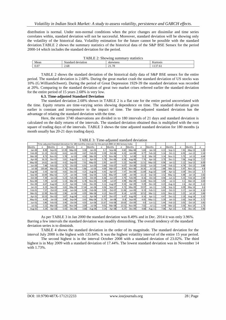
Here, the entire 3740 observations are divided in to 180 intervals of 21 days and standard deviation is

calculated on the daily returns of the intervals. The standard deviation obtained thus is multiplied with the root

square of trading days of the intervals. TABLE 3 shows the time adjusted standard deviation for 180 months (a

month usually has 20-21 days trading days).

TABLE 3: Time-adjusted standard deviation

As per TABLE 3 in Jan 2000 the standard deviation was 8.49% and in Dec. 2014 it was only 3.96%.

Barring a few intervals the standard deviation was steadily diminishing. The overall tendency of the standard

deviation series is to diminish.

TABLE 4 shows the standard deviation in the order of its magnitude. The standard deviation for the

interval July 2000 is the highest with 135.64%. It was the highest volatility interval of the entire 15 year period.

The second highest is in the interval October 2008 with a standard deviation of 23.02%. The third

highest is in May 2009 with a standard deviation of 17.44%. The lowest standard deviation was in November 14

with 1.73%.

Time-adjusted Standard deviation for 180 monthly intervals for the period 2000-14 BSE Sensex India

Months σ Months σ Months σ Months σ Months σ Months σ Months σ Months σ Months σ

Jan-00 8.49 Sep-01 12.20 May-03 3.30 Jan-05 6.7 Sep-06 4.82 May-08 5.83 Jan-10 4.22 Sep-11 7.45 May-13 5.39

Feb-00 11.13 Oct-01 6.61 Jun-03 4.67 Feb-05 3.59 Oct-06 4.22 Jun-08 8.77 Feb-10 5.14 Oct-11 6.93 Jun-13 5.54

Mar-00 8.73 Nov-01 5.78 Jul-03 4.98 Mar-05 4.79 Nov-06 2.75 Jul-08 15.9 Mar-10 3.14 Nov-11 5.75 Jul-13 4.64

Apr-00 16.23 Dec-01 5.81 Aug-03 6.11 Apr-05 5.78 Dec-06 6.58 Aug-08 7.76 Apr-10 3.79 Dec-11 7.06 Aug-13 7.57

May-00 14.61 Jan-02 4.42 Sep-03 7.91 May-05 2.95 Jan-07 5.22 Sep-08 11.51 May-10 6.96 Jan-12 5.12 Sep-13 8.09

Jun-00 7.48 Feb-02 6.75 Oct-03 6.91 Jun-05 3.66 Feb-07 6.67 Oct-08 23.02 Jun-10 5.44 Feb-12 4.74 Oct-13 3.88

Jul-00 135.64 Mar-02 5.76 Nov-03 5.86 Jul-05 4.09 Mar-07 8.93 Nov-08 16.35 Jul-10 2.89 Mar-12 5.97 Nov-13 4.8

Aug-00 5.43 Apr-02 4.65 Dec-03 4.25 Aug-05 4.45 Apr-07 7.47 Dec-08 11.69 Aug-10 3.09 Apr-12 3.59 Dec-13 3.7

Sep-00 10.09 May-02 7.27 Jan-04 9.40 Sep-05 5.02 May-07 3.69 Jan-09 13.13 Sep-10 3.52 May-12 4.48 Jan-14 3.82

Oct-00 7.39 Jun-02 5.23 Feb-04 6.55 Oct-05 6.36 Jun-07 3.75 Feb-09 8.16 Oct-10 4.94 Jun-12 5.15 Feb-14 2.94

Nov-00 7.29 Jul-02 5.13 Mar-04 6.78 Nov-05 4.39 Jul-07 4.99 Mar-09 11.69 Nov-10 5.92 Jul-12 4.1 Mar-14 3.03

Dec-00 6.67 Aug-02 4.17 Apr-04 5.81 Dec-05 5.11 Aug-07 9.33 Apr-09 9.29 Dec-10 4.23 Aug-12 2.6 Apr-14 3.12

Jan-01 6.19 Sep-02 3.65 May-04 17.44 Jan-06 4.56 Sep-07 4.72 May-09 19.97 Jan-11 5.04 Sep-12 4.09 May-14 4.6

Feb-01 7.37 Oct-02 4.44 Jun-04 6.39 Feb-06 3.95 Oct-07 11.06 Jun-09 8.19 Feb-11 6.62 Oct-12 3.17 Jun-14 4.16

Mar-01 12.99 Nov-02 2.96 Jul-04 4.95 Mar-06 4.13 Nov-07 8.14 Jul-09 10.52 Mar-11 6.01 Nov-12 3.25 Jul-14 3.84

Apr-01 10.53 Dec-02 3.87 Aug-04 4.31 Apr-06 6.97 Dec-07 6.47 Aug-09 8.16 Apr-11 4.47 Dec-12 2.19 Aug-14 3.32

May-01 4.43 Jan-03 3.40 Sep-04 3.42 May-06 11.79 Jan-08 13.8 Sep-09 4.05 May-11 5.29 Jan-13 2.63 Sep-14 3.72

Jun-01 5.86 Feb-03 3.46 Oct-04 4.03 Jun-06 15.67 Feb-08 10.63 Oct-09 4.8 Jun-11 5.44 Feb-13 3.05 Oct-14 3.85

Jul-01 5.52 Mar-03 5.00 Nov-04 3.09 Jul-06 9.01 Mar-08 13.51 Nov-09 7.02 Jul-11 4.44 Mar-13 3.56 Nov-14 1.73

Aug-01 3.24 Apr-03 5.43 Dec-04 3.68 Aug-06 3.14 Apr-08 6.27 Dec-09 4.68 Aug-11 7.06 Apr-13 4.6 Dec-14 3.96



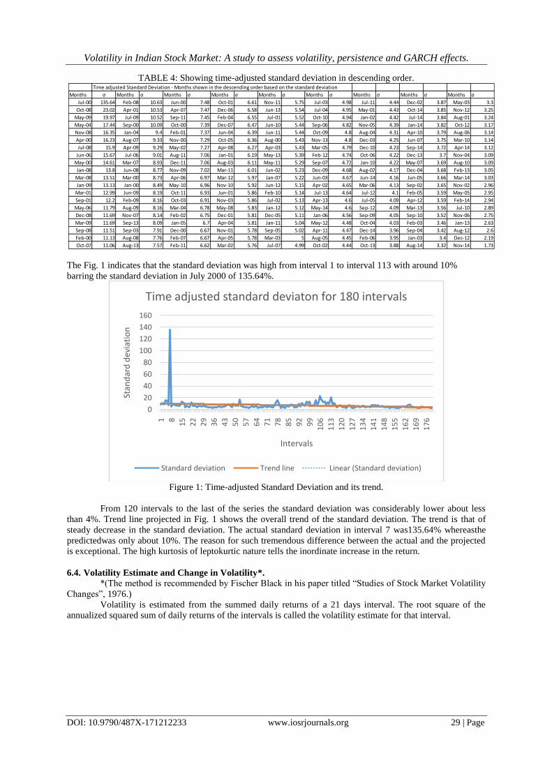
TABLE 4: Showing time-adjusted standard deviation in descending order.

The Fig. 1 indicates that the standard deviation was high from interval 1 to interval 113 with around 10%

barring the standard deviation in July 2000 of 135.64%.

Figure 1: Time-adjusted Standard Deviation and its trend.

From 120 intervals to the last of the series the standard deviation was considerably lower about less

than 4%. Trend line projected in Fig. 1 shows the overall trend of the standard deviation. The trend is that of

steady decrease in the standard deviation. The actual standard deviation in interval 7 was135.64% whereasthe

predictedwas only about 10%. The reason for such tremendous difference between the actual and the projected

is exceptional. The high kurtosis of leptokurtic nature tells the inordinate increase in the return.

6.4. Volatility Estimate and Change in Volatility*.

*(The method is recommended by Fischer Black in his paper titled “Studies of Stock Market Volatility

Changes”, 1976.)

Volatility is estimated from the summed daily returns of a 21 days interval. The root square of the

annualized squared sum of daily returns of the intervals is called the volatility estimate for that interval.

Time adjusted Standard Deviation - Months shown in the descending order based on the standard deviation

Months σ Months σ Months σ Months σ Months σ Months σ Months σ Months σ Months σ

Jul-00 135.64 Feb-08 10.63 Jun-00 7.48 Oct-01 6.61 Nov-11 5.75 Jul-03 4.98 Jul-11 4.44 Dec-02 3.87 May-03 3.3

Oct-08 23.02 Apr-01 10.53 Apr-07 7.47 Dec-06 6.58 Jun-13 5.54 Jul-04 4.95 May-01 4.43 Oct-14 3.85 Nov-12 3.25

May-09 19.97 Jul-09 10.52 Sep-11 7.45 Feb-04 6.55 Jul-01 5.52 Oct-10 4.94 Jan-02 4.42 Jul-14 3.84 Aug-01 3.24

May-04 17.44 Sep-00 10.09 Oct-00 7.39 Dec-07 6.47 Jun-10 5.44 Sep-06 4.82 Nov-05 4.39 Jan-14 3.82 Oct-12 3.17

Nov-08 16.35 Jan-04 9.4 Feb-01 7.37 Jun-04 6.39 Jun-11 5.44 Oct-09 4.8 Aug-04 4.31 Apr-10 3.79 Aug-06 3.14

Apr-00 16.23 Aug-07 9.33 Nov-00 7.29 Oct-05 6.36 Aug-00 5.43 Nov-13 4.8 Dec-03 4.25 Jun-07 3.75 Mar-10 3.14

Jul-08 15.9 Apr-09 9.29 May-02 7.27 Apr-08 6.27 Apr-03 5.43 Mar-05 4.79 Dec-10 4.23 Sep-14 3.72 Apr-14 3.12

Jun-06 15.67 Jul-06 9.01 Aug-11 7.06 Jan-01 6.19 May-13 5.39 Feb-12 4.74 Oct-06 4.22 Dec-13 3.7 Nov-04 3.09

May-00 14.61 Mar-07 8.93 Dec-11 7.06 Aug-03 6.11 May-11 5.29 Sep-07 4.72 Jan-10 4.22 May-07 3.69 Aug-10 3.09

Jan-08 13.8 Jun-08 8.77 Nov-09 7.02 Mar-11 6.01 Jun-02 5.23 Dec-09 4.68 Aug-02 4.17 Dec-04 3.68 Feb-13 3.05

Mar-08 13.51 Mar-00 8.73 Apr-06 6.97 Mar-12 5.97 Jan-07 5.22 Jun-03 4.67 Jun-14 4.16 Jun-05 3.66 Mar-14 3.03

Jan-09 13.13 Jan-00 8.49 May-10 6.96 Nov-10 5.92 Jun-12 5.15 Apr-02 4.65 Mar-06 4.13 Sep-02 3.65 Nov-02 2.96

Mar-01 12.99 Jun-09 8.19 Oct-11 6.93 Jun-01 5.86 Feb-10 5.14 Jul-13 4.64 Jul-12 4.1 Feb-05 3.59 May-05 2.95

Sep-01 12.2 Feb-09 8.16 Oct-03 6.91 Nov-03 5.86 Jul-02 5.13 Apr-13 4.6 Jul-05 4.09 Apr-12 3.59 Feb-14 2.94

May-06 11.79 Aug-09 8.16 Mar-04 6.78 May-08 5.83 Jan-12 5.12 May-14 4.6 Sep-12 4.09 Mar-13 3.56 Jul-10 2.89

Dec-08 11.69 Nov-07 8.14 Feb-02 6.75 Dec-01 5.81 Dec-05 5.11 Jan-06 4.56 Sep-09 4.05 Sep-10 3.52 Nov-06 2.75

Mar-09 11.69 Sep-13 8.09 Jan-05 6.7 Apr-04 5.81 Jan-11 5.04 May-12 4.48 Oct-04 4.03 Feb-03 3.46 Jan-13 2.63

Sep-08 11.51 Sep-03 7.91 Dec-00 6.67 Nov-01 5.78 Sep-05 5.02 Apr-11 4.47 Dec-14 3.96 Sep-04 3.42 Aug-12 2.6

Feb-00 11.13 Aug-08 7.76 Feb-07 6.67 Apr-05 5.78 Mar-03 5 Aug-05 4.45 Feb-06 3.95 Jan-03 3.4 Dec-12 2.19

Oct-07 11.06 Aug-13 7.57 Feb-11 6.62 Mar-02 5.76 Jul-07 4.99 Oct-02 4.44 Oct-13 3.88 Aug-14 3.32 Nov-14 1.73

0

20

40

60

80

100

120

140

160

1 8

15

22

29

36

43

50

57

64

71

78

85

92

99

10

6

11

3

12

0

12

7

13

4

14

1

14

8

15

5

16

2

16

9

17

6

Stan

dar

d d

evia

tio

n

Intervals

Time adjusted standard deviaton for 180 intervals

Standard deviation Trend line Linear (Standard deviation)



TABLE 5: Showing the volatility estimate & volatility change

TABLE 5 shows 25 intervals of volatility estimate and change in volatility. The volatility of the first

interval January 2000 was 10%. The standard deviation as per TABLE 3 for January 2000 was 8.49%. The

volatility estimate for Feb. 2000 was 18% whereas the standard deviation for the same interval was 11.13%. The

volatility estimate for the interval March 2000 was 28%. But the standard deviation for the same interval as per

TABLE 3 was 8.73%. In this way standard deviation as per TABLE 3 more or less resembles the volatility

estimate shown in TABLE 5.

Going through TABLE 5 it can be understood that there is a relationship between the summed returns

and volatility estimate. When the summed return was -2.87 in Jan-2000 the volatility estimate against that was

10%. When the summed return increased to 5.13% in Feb-2000 the volatility estimate also increased to 18%.

For 278% increase in the summed returns the volatility increases by 80%. The change in volatility is

80% during this period. In March 2000 the summed return decreases to -8.15%. Consequent to that the volatility

estimate though increases to 28%, the rate of change in volatility reduced to 55%. In July 2000 the summed

return was 57.26%, against which the volatility estimate was 198%. From this it can be inferred that the summed

returns of intervals and volatility estimates are positively correlated. When the summed returns are regressed

with a constant and volatility estimate to find the intimacy, by making the volatility estimate as the dependent

variable (Y) and the summed returns as the independent variable (X), the coefficients obtained are as follows.

TABLE 6: Regression Coefficients

TABLE 6 implies that the volatility estimate will be 2.12 times that of the summed returns of the

intervals. The P- value for the intercept and beta coefficient both are less than 5%. Therefore they are

significant. As the P-value is less than 5%the null hypothesis that the coefficient b1=0 is rejected and the

alternative hypothesis that beta> 0 is accepted. Hence, it can be deduced that the relation between the summed

returns and volatility estimate is very strong.

TABLE 5 also shows the change in volatility. The estimated volatility as per the TABLE5 never

remains constant. It changes for every change in the summed returns. The change in volatility in the first

Squared Annualise Volatility Volatility

Summed Summed Value Estimate Change

Interval Return Return

Jan.00 -2.87% 0.08% 0.99% 10%

Feb.00 5.13% 0.26% 3.16% 18% 79%

Mar.00 -8.15% 0.66% 7.97% 28% 59%

Apr.00 -5.84% 0.34% 4.09% 20% -28%

May-00 -3.88% 0.15% 1.81% 13% -34%

Jun-00 7.15% 0.51% 6.13% 25% 84%

Jul.00 57.26% 32.79% 393.45% 198% 701%

Aug.00 4.65% 0.22% 2.59% 16% -92%

Sep.00 -8.51% 0.72% 8.69% 29% 83%

Oct.00 -9.43% 0.89% 10.67% 33% 11%

Nov.00 7.72% 0.60% 7.15% 27% -18%

Dec.00 -0.42% 0.00% 0.02% 1% -95%

Jan.01 8.73% 0.76% 9.15% 30% 1939%

Feb.01 -1.61% 0.03% 0.31% 6% -82%

Mar.01 -15.52% 2.41% 28.90% 54% 864%

Apr.01 -1.85% 0.03% 0.41% 6% -88%

May.01 3.24% 0.11% 1.26% 11% 75%

Jun.01 -4.78% 0.23% 2.74% 17% 48%

Jul.01 -3.59% 0.13% 1.55% 12% -25%

Aug.01 -2.52% 0.06% 0.76% 9% -30%

Sep.01 -13.56% 1.84% 22.06% 47% 438%

Oct.01 6.36% 0.40% 4.85% 22% -53%

Nov.01 9.68% 0.94% 11.24% 34% 52%

Dec.01 -0.61% 0.00% 0.04% 2% -94%

Jan.02 1.59% 0.03% 0.30% 6% 163%

Coefficients Standard Error t Stat P-value

Intercept 0.24569247 0.051567817 4.764454 0.00083

X Variable 12.11718588 0.38785659 5.458682 0.000151



instance was 79%, then, 59%, then by -28%, and then by -34% and so on. The rate of change in volatility is not

constant. Regressing the rate of change and the summed return it can be seen that for a 1% change in the

summed return the volatility changes by 2.5% negatively. There is a very strong relation between the summed

return and the change in volatility.

6.5. GARCH (1,1) Model

Standard deviation or variance is always constant. When standard deviation is used to represent

volatility the assumption is that the volatility is also constant over a period. If volatility changes from time to

time, especially it is true in the case of time-varying series, standard deviation fails. Equity returns are time-

varying series. Moreover, the studies reveal that equity returns series are serially correlated. There are evidences

for interdependency within the return series. TABLE 2 shows non-normality of equity returns due to the

presence of large amount skewness and kurtosis. Since returns are interdependent within series, volatility too

becomes interdependent. Due to dependency, it becomes true that today’s return dependent upon the volatility of

yesterday. Similarly, Current volatility may depend upon previous day’s volatility. Accordingly, current return

is conditional upon the previous day’s return and current volatility is conditional upon previous day’s volatility.

This situation is called Generalized Auto Regressive Conditionally Heteroscedastic (GARCH) effect in the

series. In terms of GARCH (1,1) terms-

Yt =(Yt/Yt-1) (9)

Yt is current return and Yt-1 is the return of the previous (t-1) period.

Likewise,

σ2t=(σ

2t / σ

2t-1 ) (10)

Where, σ2t is current variance and σ

2t-1 is the conditional variance.

In such cases volatility is conditional and will change conditionally throughout the period in different

magnitude. This hetroscedascticity of equity returns is governed by mainly three factors viz., 1) Long-run

variance, 2) Previous day’s returns, and 3) Previous day’s variance.

Hence conditional variance is the measure of stock volatility which can be put in GARCH terms as

equation (8). GARCH model is relevant when there is excessive volatility clustering and volatility dependence.

Figure 2:Behaviour of residuals

It can be noticed from Fig.2 that the volatility in residuals is dissimilar. There is slight volatility

clustering in the distribution of the residuals. From day 1 to 141 the volatility is low. During this period low

volatility is followed by low volatility for a prolonged period up to 141 days. From 141 to 142 days the volatility

is very high. But this high volatility is not followed for a prolonged period. It is only for two days. From 142 to

1950th

day low volatility is followed by low volatility for a prolonged period. From 1951 to 2401st day high

volatility is followed by high volatility. From 2401 to 3739th

day low volatility is followed by low volatility.

Thus volatility has 5 segments. They are day 1 to 141, day 141 to 142, day 142 to 1950, day 1951 to 2401, and

day 2401 to 3739. The first spell is characterized by low volatility followed by low volatility for a long period,

the second by high volatility for a short period, the third by low volatility followed by low volatility for

prolonged period, the fourth by relatively high volatility followed by high volatility and fifth by low volatility

followed by low volatility for a prolonged period.

-100.00%

-80.00%

-60.00%

-40.00%

-20.00%

0.00%

20.00%

40.00%

60.00%

80.00%

100.00%

1

15

7

31

3

46

9

62

5

78

1

93

7

10

93

12

49

14

05

15

61

17

17

18

73

20

29

21

85

23

41

24

97

26

53

28

09

29

65

31

21

32

77

34

33

35

89

Res

idu

als

No. of Obsevation

Volatility clustering in residuals



The low/ high volatility followed by low / high volatility for a prolonged period indicates volatility

clustering and volatility interdependency and persistence. This is an evidence of the prevalence of conditional

volatility or GARCH effect in Indian stock market.

When mean and variance equations of the GARCH (1,1) model are solved and maximized the log

likelihood, the parameters are estimated as under:

TABLE7:GARCH(1,1) Parameters Parameters Coefficients

ω 0.00028565

α1 0.28657148

b1 0.24478029

(α1+ b1)= λ 0.53135177

Unconditional variance 0.00071906

TABLE 7 provides the estimated GARCH (1,1) parameters. The constraints of GARCH (1,1)

parameters are

α1>0

b1> 0

(α1+ b1)= λ< 1

Here, α1 is the coefficient of 1 lag squared residuals Ԑ²t-1

b1 is the coefficient of 1 lag variance σ²t-1

λis the sum of α1 and b1 representing volatility persistence.

Unconditional volatility (VL) = ω

1−α−b =

ω

1−λ(11)

Conditional volatility = σ²t=VL*λ(12)

TABLE 7 shows that the parameters are above 0 and the sum of α1 and b1 is less than 1. The parameters

tell the quantum of conditional volatility in the variance of returns. If alpha increases beta will reduce and vice

versa. If λ, the sum of α1and b1 nears 1 it signals extreme conditional volatility persistence on current

unconditional variance. If λ is lower persistence can be said lower. If λ is higher persistence is higher. If λ is 1 as

per equation (11) unconditional volatility becomes zero. In that case the whole volatility will be conditional.

TABLE 7 shows that λis 0.53135177. It implies that the past shocks only moderately influence the

current variance. The current variance has both the components of unconditional and conditional variances in an

equal way.The conditional part of current variance as per TABLE 7 is 53% of unconditional variance.

VII. Conclusion This paper attempted to study the volatility in Indian stock market with the daily data of S&P BSE

Sensex for a period of 15 years from 2000 to 2014 with a total of 3740 observations. BSE Sensex was chosen to

represent Indian stock market. The study has found that there is considerable difference between the quantitative

change and percentage change in the Sensex. Keeping aside a few days of exceptional behavior due to excess

skewness and excess kurtosis the percentage change in the index is below 8%. The standard deviation for the

entire period is considerably lower, less than 3%. The time-adjusted standard deviation for 180 intervals of 21

days is almost similar to the percentage change in the index. The time-adjusted standard deviation showed a

trend of steady decline from the initial periods’ 10% to below 4% ending with 1.73%. Volatility estimate based

on the summed daily returns show volatility similar to time-adjusted standard deviation. But the relationship

between the summed returns and the volatility estimate is found very strong when they are regressed. Hence it

becomes possible to predict the volatility if daily returns are available. There are enough evidences for the

presence of heteroscedasticity in the equity returns of Indian stock market. When residuals are examined it is

found that there is volatility clustering. Low volatility is followed by low volatility and high volatility is

followed by high volatility for a prolonged period. Indian stock market has GARCH effect. The GARCH

parameters show evidences for moderate volatility persistence in the equity returns.

References [1]. Engle, R.F., 1982, Autoregressive conditional heteroskedasticity with estimates of the variance of U.K. inflation, Econometrica 50,

987-1008.

[2]. Tim bollerslev, “Generalized Autoregressive Conditional Heteroskedasticity”,University of California at San Diego, La Jolla, CA

92093, USA,Institute of Economics, University of Aarhus, Denmark, February 1986. [3]. Tagliafichi Ricardo A. “Betas calculated with GARCH models provides new parameters for a portfolio selection with an efficient

frontier”, ASTIN Colloquium, Cancun, Mexico, 2002.

[4]. Tim bollerslev, “Generalized Autoregressive Conditional Heteroskedasticity”,University of California at San Diego, La Jolla, CA 92093, USA,Institute of Economics, University of Aarhus, Denmark, February 1986.



[5]. Timothy J. Brailsford, “The Empirical Relationship Between Trading Volume, Returns AndVolatility”, Department of Accounting

and Finance, University of Melbourne, Parkville 3052, Australia, December 1994.

[6]. Carla Inclan and George C. Tiao, “Use of Cumulative Sums of Squares for Retrospective Detection of Changes of Variance”,

Journal of the American Statistical Association, Vol. 89, No. 427. (Sep., 1994), pp. 913-923. [7]. DimaAlberg, HaimShalit, and Rami Yosef, “Estimating stock market volatility using asymmetric GARCH models”, Applied

Financial Economics, 2008, 18, 1201–1208.

[8]. Kenneth R.French, G.WilliamSchwert, Robert F.Stambaugh, “Expected Stock Returns and Volatility”, Journal of Financial Economics, 1987, Volume 19, Issue 1, pp. 3-29.

[9]. ZsuzsannaHorv´ath and Ryan Johnston, “GARCH Time Series Process”, Econometrics 7590, Projects 2 and 3.

[10]. Pankunni.V, “Beta Analysis of Equity Returns: An Empirical Study about the Significance of Beta and Its Linearity.” IOSR Journal of Business and Management (IOSR-JBM), e-ISSN: 2278-487X, p-ISSN: 2319-7668. Volume 17, Issue 4.Ver. II (Apr. 2015), PP

10-22, DOI No. 10.9790/487X-16625299.

[11]. M. T. Raju, Anirban Ghosh, “Stock Market Volatility – An International Comparison”, Securities and Exchange Board of India, Working Paper Series No. 8, April 2004.

[12]. G.WilliamSchwert, “Stock Market Volatility: Ten years after the crash”, National Bureau of Economic Research, 1050

Massachusettes Avenue, Cambridge, 1998. [13]. AmitaBatra, “Stock Return Volatility Patterns In India”, Indian Council for Research on International Economic Relations, Core-

6A, 4th Floor, India Habitat Centre, Lodi Road, New Delhi-110 003, March, 2004.

[14]. DebeshBhowmik, “Stock Market Volatility: An Evaluation”, (International Institute for Development Studies,Kolkata International

Journal of Scientific and Research Publications, Volume 3, Issue 10, October 2013, ISSN 2250-3153.

[15]. Giorgio De Santis and SelhattinImrohoroglu, “ Stock Returns and Volatility in Emerging Financial Markets”, Discussion paper 93,

University of Southern California. July 1994. [16]. Fischer Black, “ Studies of Stock Market Volatility Changes”, Proceedings of American Statistical Association, Business and

Economic Statistics Section, 1976, 177-81

[17]. Reena Aggarwal, Carla Inclan and Ricardo Leal, “ Volatility in Emergin Markets”, Journal of Financial and Quantitative analysis 33-35, 1999.

[18]. Reider, Rob. "Volatility forecasting I: GARCH models." New York (2009).

[19]. Tauchen, George, “The Relationship Between Trading Volume and Jump Processes in Financial Markets” Diss. Duke University, Durham, 2009.

Date post:	17-Feb-2016
Category:	Documents
Upload:	iosrjournal
View:	9 times
Download:	3 times

Volatility in Indian Stock Market: A study to assess volatility, persistence and GARCH effects.

Documents