*Robert S. Pindyck, the Bank of Tokyo-Mitsubishi Professor of Economics and Finance in theSloan School of Management at the Massachusetts Institute of Technology (M.I.T.), is also a Re-search Associate of the National Bureau of Economic Research and a Fellow of the EconometricSociety. The author, who received a Ph.D. in economics from M.I.T., has been a visiting professorat both Tel Aviv and Harvard Universities, a coeditor of The Review of Economics and Statistics,and a consultant to a large number of public and private organizations. Dr. Pindyck�s research andwriting have covered topics in microeconomics and industrial organization, the behavior of re-source and commodity markets, financial markets, and econometric modeling and forecasting. Alongwith numerous academic journal articles, he has authored or coauthored seven books, including thewidely used texts Econometric Models and Economics Forecasts (McGraw-Hill), Microeconomics(Prentice-Hall), and Investment under Uncertainty (Princeton University Press). His recent work ineconomics and finance has examined the role of research and development and the value of patents,determinants of market structure and market power, the dynamics of commodity spot and futuresmarkets, and criteria for investing in risky projects. The author is grateful to M.I.T.�s Center forEnergy and Environmental Policy Research for its financial support of the research leading to thispaper, to Mr. Scott Byrne and the New York Mercantile Exchange for providing futures marketdata, and to Martin Minnoni for his outstanding research assistance.
This paper examines the behavior of natural-gas and crude-oil price volatility inthe United States since 1990. Prices of crude oil and especially natural gas
rose sharply (but temporarily) during late 2000, and natural gas trading was buf-feted by the collapse of Enron in late 2001, suggesting to some that volatility inthese markets has increased. Whether or not this is true, volatility has been highand (like prices themselves) fluctuates dramatically.
Understanding volatility in natural gas and crude oil markets is important forseveral reasons. Persistent changes in volatility can affect the risk exposure of
2 THE JOURNAL OF ENERGY AND DEVELOPMENT
producers and industrial consumers of natural gas and oil; they can alter the incen-tives to invest in natural gas and oil inventories and facilities for production andtransportation. Likewise, volatility is a key determinant of the value of commodity-based contingent claims, whether financial or �real.� Thus, the behavior of volatilityis significant for derivative valuation, hedging decisions, and decisions to invest inphysical capital tied to the production or consumption of natural gas or oil.
In addition, volatility plays a role in the short-run market dynamics for naturalgas and oil. As discussed in my recent paper, volatility can affect the demand forstorage and also can impact the total marginal cost of production by affecting thevalue of firms� operating options and thereby the opportunity cost of current pro-duction.1 In particular, greater volatility should lead to an increased demand forstorage and an increase in both spot prices and marginal convenience yield.2 Thus,changes in volatility can help explain changes in these other variables.
With this in mind, the following questions are addressed. First, has natural-gasand/or crude-oil price volatility changed significantly since 1990 and, in particular,are there measurable trends in volatility? Related to this, have the events surround-ing the collapse of Enron affected volatility, i.e., was there a significant short-termincrease in volatility around the time of the collapse? Second, are natural gas andcrude oil volatilities interrelated, i.e., can changes in one help predict changes inthe other? Third, although volatility clearly fluctuates over time, how persistentare the changes? If changes are very persistent, then they will lead to changes inthe prices of options and other derivatives (real or financial) that are tied to theprices of these commodities. However, if changes in volatility are highly transi-tory, they should have little or no impact on market variables or on real and financialoption values. Finally, extending an earlier analysis,3 the question is revisited ofwhether changes in volatility are predictable.
To address these questions, daily futures price data for natural gas and crude oilare used to infer daily spot prices and daily values of the net marginal convenienceyield. From the log price changes (adjusted for non-trading days) and marginalconvenience yield, daily and weekly returns from holding each commodity arecalculated. Volatility then is estimated in three different ways.
First, using a five-week overlapping window, weekly series for price volatilityare estimated by calculating sample standard deviations of (adjusted) daily logprice changes. As J. Campbell et al. point out in their study of stock price volatil-ity, in addition to its simplicity, this approach has the advantage that it does notrequire a parametric model describing the evolution of volatility over time.4 Sec-ond, series for conditional volatility are estimated by estimating generalizedautoregressive conditional heteroscedasticity (GARCH) models of the weeklyreturns on the commodities; the volatility estimates from these models are com-pared to the sample standard deviations.5 Third, a daily series for conditionalvolatility is estimated by using GARCH models of the daily returns on thecommodities.6
NATURAL GAS AND OIL MARKET VOLATILITY 3
The behavior of volatility is studied in two different ways. First, using theestimated weekly sample standard deviations, I test for the presence of time trends;I test whether volatility was significantly greater during the period of the Enroncollapse; and I examine whether gas (oil) volatility is a significant predictor of oil(gas) volatility. These series also are used to estimate the persistence of changes involatility. Second, these same questions are addressed using weekly and dailyGARCH models of commodity returns. For example, I test whether a time trend ora dummy variable for the Enron period is a significant explanator of volatility(and/or returns) in the GARCH framework. Likewise, the estimated coefficientsfrom the variance equation of each GARCH model provide a direct estimate of thepersistence of volatility shocks.
While the focus here is on prices, there are other measures of volatility. Puttingaside issues of data availability, one could examine instead the volatility of con-sumption, production, or inventories. That would indeed be useful if the objectivewas to explain the determinants of inventory demand, e.g., the role of productionand/or consumption smoothing and production-cost smoothing.7 My concern, how-ever, is with the overall market, and the spot price is the best single statistic formarket conditions. Spot price volatility reflects the volatility of current as well asexpected future values of production, consumption, and inventory demand.8
My results can be summarized as follow. (1) There is a statistically significantpositive trend in volatility for natural gas (but not for crude oil). However, thistrend is of little economic importance; over a 10-year period, it amounts to about a3-percent increase in volatility. (2) There is no statistically significant increase involatility during the period of the Enron collapse. (3) The evidence is mixed as tothe interrelationship between crude oil and natural gas returns and volatilities. Usingdaily data, crude oil returns are a significant predictor of natural gas returns (butnot the other way around), and crude oil volatility is a significant predictor ofnatural gas volatility. Using weekly data, however, these results are less clear-cut.(4) Shocks to volatility are generally short-lived for both natural gas and crude oil.Volatility shocks decay (i.e., there is reversion to the mean) with a half-life of about5 to 10 weeks.
In the next section, the data and the calculation of returns and weekly samplestandard deviations are discussed. All of the empirical work is presented in thesubsequent section on the behavior of volatility and prices, which is followed bythe conclusions.
The Data
To begin, natural-gas and crude-oil futures price data are utilized covering theperiod May 2, 1990, through February 26, 2003. (The start date was constrainedby the beginning of active trading in natural gas futures.) To obtain a weekly series
4 THE JOURNAL OF ENERGY AND DEVELOPMENT
for volatility, the sample standard deviations of adjusted daily log price changes inspot and futures prices are used. As discussed below, I also obtain estimates ofconditional volatility from GARCH models of weekly and daily returns.
Spot Prices and Weekly Volatility: For each commodity, daily futures settle-ment price data were compiled for the nearest contract (often the spot contract), thesecond-nearest, and the third-nearest. These prices are denoted by F1, F2, and F3.The spot price can be measured in three alternative ways. First, one can use cashprices, purportedly reflecting actual transactions. But daily cash price data usuallyare not available, and a cash price can include discounts and premiums that resultfrom relationships between buyers and sellers; it need not reflect precisely thesame product (including delivery location) specified in the futures contract. Asecond approach is to use the price of the spot futures contract, i.e., the contractthat expires in month t. But the spot contract often expires before the end of themonth, and active spot contracts do not always exist for each month.
The third approach, which is used here, is to infer a spot price from the nearestand the next-to-nearest active futures contracts. This is done for each day by ex-trapolating the spread between these contracts backward to the spot month as follows:
1t0 n/ntttt )2F/1F(1FP = (1)
where Pt is the spot price on day t; F1
t and F2
t are the prices on the nearest and next-
to-nearest futures contracts, respectively; and n0t and n
1 are the number of days
from t to the expiration of the first contract and the number of days between theexpiration dates for the first and second contracts, respectively.
Given these daily estimates of spot prices, I compute weekly estimates of vola-tility. To do this, one must take into account weekends and other non-trading days.If the spot price followed a geometric Brownian motion, this could be done simplyby dividing the log price changes by the square root of the number of interveningdays (e.g., three days in the case of a weekend), and then calculating the samplevariance. However, as is well known, on average the standard deviation of n-daylog price changes is significantly less than n times the standard deviation of one-day log price changes, when n includes non-trading days.9 To deal with this, thedaily price data are sorted by intervals, according to the number of days since thelast trading day. For example, if there were no holidays in a particular period,prices for Tuesday, Wednesday, Thursday, and Friday would all be classified ashaving an interval of one day, and Monday would be assigned an interval of threedays because of the weekend. Because of holidays, some prices are assigned tointervals of two, four, or even five days (if a weekend was followed by a two-dayholiday).
For each interval set, the sample standard deviation of log price changes is cal-culated for the entire sample for each commodity. Letting nS� denote this sample
NATURAL GAS AND OIL MARKET VOLATILITY 5
standard deviation for log price changes over an interval of n days, the �effective�daily log price change is computed as:
1n
nt
S�/S�)PlogP(log −ττ −=δ . (2)
For each week, I then compute a sample variance and corresponding samplestandard deviation using these �effective� daily log price changes for that weekand the preceding four weeks:
∑=τ
τ δ−δ−
=σN
1
2ttt )(
1N
1� , (3)
where N is the number of �effective� days in the five-week interval. Equation (3)gives the sample standard deviation of daily percentage price changes; to put it inweekly terms, one multiplies by 4/30 = 5.7 . The resulting weekly series is ameasure of volatility, tσ .
Daily and Weekly Returns: An important advantage of using the weekly esti-mates of volatility discussed above (besides its simplicity) is that it does not requirea parametric model of the evolution of volatility over time. However, there aredisadvantages as well. The first is that the use of overlapping intervals introducesserial correlation as an artifact, which makes it more difficult to discern the time-series properties of volatility. A second disadvantage is that even the use of afive-week interval yields imprecise estimates of the standard deviation. Hence, Ialso estimate volatility from GARCH models of commodity returns. These modelscan include parameters that test for time variation (such as trends or an �Enroneffect�) and have the additional advantage that the time-series properties of volatil-ity (the ARCH and GARCH components, which determine the persistence ofvolatility shocks) are estimated along with the volatility itself.
Marginal Convenience Yield: One part of the total return on the commodity isthe net marginal convenience yield, tψ , i.e., the value of the flow of production-and delivery-facilitating services from the marginal unit of inventory, net of stor-age costs. Net marginal convenience yield can be measured from spot and futuresprices as
tψ = (1+rt)P
t � F
1t, (4)
where F1t is the futures price at time t for a contract maturing at time t + 1, and r
t is
6 THE JOURNAL OF ENERGY AND DEVELOPMENT
the one-period riskless interest rate. The values of tψ are calculated for everytrading day using the futures price corresponding as closely as possible to a one-month interval from the spot price. (When there are few or no trades of the nearestfutures contract, as sometimes occurs with natural gas, the next-to-nearest contractis used instead.) Further, I employed the yield on three-month Treasury bills, ad-justed for the number of days between P
t and F
1t, for the interest rate r
t.
In what follows, both daily and weekly series are used for the marginal conve-nience yield, so tψ is converted into daily terms, i.e., dollars per unit of commodityper day. For days followed by another trading day (e.g., a Monday), one simplydivides the values of tψ calculated above by the number of days between P
t and
F1t. For days followed by n non-trading days, these values are multiplied by n+1.
(Thus for a Friday, which is typically followed by n = 2 non-trading days, theconvenience yield is the flow of value from holding a marginal unit of inventoryover the next three days.) This daily series is used to compute daily returns fromholding the commodity.
To obtain a weekly series, I use the calculated values of tψ for the Wednesdayof each week, and multiply those values by seven so that the convenience yield ismeasured in dollars per unit of commodity per week. (If Wednesday is a holiday,Thursday�s price is used.) This weekly series then is utilized to calculate weeklyreturns from holding the commodity.
Calculating Returns: The total return from holding a unit of a commodity overone period is the capital gain or loss over that period, plus the �dividend,� which isthe net marginal convenience yield, i.e., the flow of benefits to producers or con-sumers from holding the marginal unit of inventory, net of storage costs. I calculatea series of daily (weekly) returns by summing the �effective� daily log price changesover each day (week) and adding to this the estimate of daily (weekly) conve-nience yield. The weekly return, for example, is calculated as:
∑=τ
ψ+δ=T
1tttR (5)
where τδ is given by equation (2) and T is the number of days in the week. Aseries for the daily return is calculated by using the effective daily log price changefor each effective trading day and adding the daily flow of marginal convenienceyield. (Because effective trading days are utilized, the daily series will have about20 data points per month.)
The Behavior of Volatility and Prices
To examine the behavior of natural-gas and crude-oil price volatility, I first usethe weekly time series of sample standard deviations of adjusted log price changes.
NATURAL GAS AND OIL MARKET VOLATILITY 7
These time series show little evidence of either a trend in volatility or a significantincrease in volatility during the period of the Enron collapse. In addition, changesin volatility appear to be highly transitory, with a half-life of several weeks. As analternative way of measuring volatility, GARCH models of the weekly returns toholding the commodity are estimated, which yields estimates of the weekly condi-tional standard deviations. I test for changes in volatility over time by introducinga time trend and an Enron dummy variable in the variance equations of the GARCHmodels, and obtain results that are similar to those obtained from the weekly samplestandard deviations. The daily adjusted return series is used to estimate dailyGARCH models. These provide estimates of conditional standard deviations on adaily basis that also are used to test for time trends and an Enron effect and toestimate the persistence of changes in volatility.
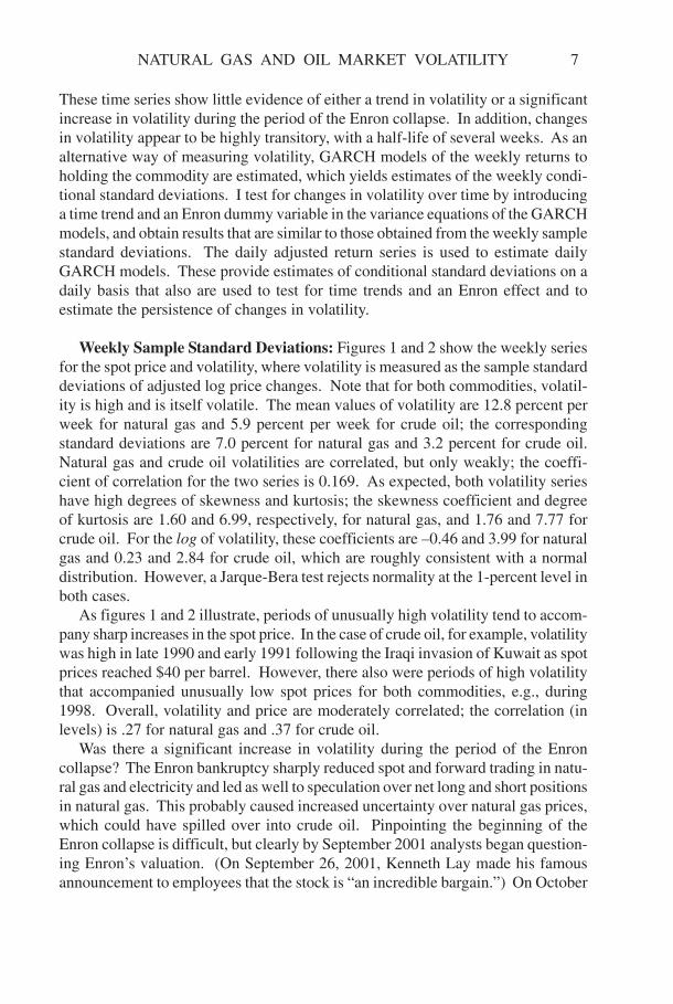
Weekly Sample Standard Deviations: Figures 1 and 2 show the weekly seriesfor the spot price and volatility, where volatility is measured as the sample standarddeviations of adjusted log price changes. Note that for both commodities, volatil-ity is high and is itself volatile. The mean values of volatility are 12.8 percent perweek for natural gas and 5.9 percent per week for crude oil; the correspondingstandard deviations are 7.0 percent for natural gas and 3.2 percent for crude oil.Natural gas and crude oil volatilities are correlated, but only weakly; the coeffi-cient of correlation for the two series is 0.169. As expected, both volatility serieshave high degrees of skewness and kurtosis; the skewness coefficient and degreeof kurtosis are 1.60 and 6.99, respectively, for natural gas, and 1.76 and 7.77 forcrude oil. For the log of volatility, these coefficients are �0.46 and 3.99 for naturalgas and 0.23 and 2.84 for crude oil, which are roughly consistent with a normaldistribution. However, a Jarque-Bera test rejects normality at the 1-percent level inboth cases.
As figures 1 and 2 illustrate, periods of unusually high volatility tend to accom-pany sharp increases in the spot price. In the case of crude oil, for example, volatilitywas high in late 1990 and early 1991 following the Iraqi invasion of Kuwait as spotprices reached $40 per barrel. However, there also were periods of high volatilitythat accompanied unusually low spot prices for both commodities, e.g., during1998. Overall, volatility and price are moderately correlated; the correlation (inlevels) is .27 for natural gas and .37 for crude oil.
Was there a significant increase in volatility during the period of the Enroncollapse? The Enron bankruptcy sharply reduced spot and forward trading in natu-ral gas and electricity and led as well to speculation over net long and short positionsin natural gas. This probably caused increased uncertainty over natural gas prices,which could have spilled over into crude oil. Pinpointing the beginning of theEnron collapse is difficult, but clearly by September 2001 analysts began question-ing Enron�s valuation. (On September 26, 2001, Kenneth Lay made his famousannouncement to employees that the stock is �an incredible bargain.�) On October
8 THE JOURNAL OF ENERGY AND DEVELOPMENT
Figure 1NATURAL GAS: WEEKLY SPOT PRICE AND VOLATILITY, 1990-2002
0
2
4
6
8
10
12
.0
.1
.2
.3
.4
.5
1990 1992 1994 1996 1998 2000 2002
Volatility
Spot price
In Percent per Week
In Dollars per Thousand Cubic Feet
Figure 2CRUDE OIL: WEEKLY SPOT PRICE AND VOLATILITY, 1990-2002
10
20
30
40
50
.00
.05
.10
.15
.20
.25
1990 1992 1994 1996 1998 2000 2002
Volatility
Spot price
In Percent per Week
In Dollars per Barrel
NATURAL GAS AND OIL MARKET VOLATILITY 9
16, 2001, Enron reported a $638-million third-quarter loss and disclosed a $1.2-billion reduction in shareholder equity. Further financial statement revisions wereannounced during October and November; Enron filed for Chapter 11 bankruptcyprotection on December 2.
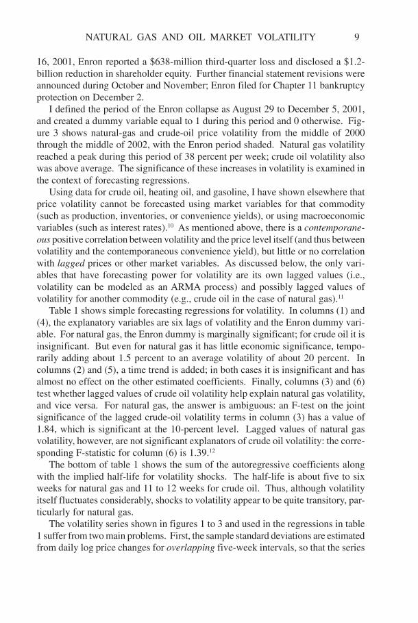
I defined the period of the Enron collapse as August 29 to December 5, 2001,and created a dummy variable equal to 1 during this period and 0 otherwise. Fig-ure 3 shows natural-gas and crude-oil price volatility from the middle of 2000through the middle of 2002, with the Enron period shaded. Natural gas volatilityreached a peak during this period of 38 percent per week; crude oil volatility alsowas above average. The significance of these increases in volatility is examined inthe context of forecasting regressions.
Using data for crude oil, heating oil, and gasoline, I have shown elsewhere thatprice volatility cannot be forecasted using market variables for that commodity(such as production, inventories, or convenience yields), or using macroeconomicvariables (such as interest rates).10 As mentioned above, there is a contemporane-ous positive correlation between volatility and the price level itself (and thus betweenvolatility and the contemporaneous convenience yield), but little or no correlationwith lagged prices or other market variables. As discussed below, the only vari-ables that have forecasting power for volatility are its own lagged values (i.e.,volatility can be modeled as an ARMA process) and possibly lagged values ofvolatility for another commodity (e.g., crude oil in the case of natural gas).11
Table 1 shows simple forecasting regressions for volatility. In columns (1) and(4), the explanatory variables are six lags of volatility and the Enron dummy vari-able. For natural gas, the Enron dummy is marginally significant; for crude oil it isinsignificant. But even for natural gas it has little economic significance, tempo-rarily adding about 1.5 percent to an average volatility of about 20 percent. Incolumns (2) and (5), a time trend is added; in both cases it is insignificant and hasalmost no effect on the other estimated coefficients. Finally, columns (3) and (6)test whether lagged values of crude oil volatility help explain natural gas volatility,and vice versa. For natural gas, the answer is ambiguous: an F-test on the jointsignificance of the lagged crude-oil volatility terms in column (3) has a value of1.84, which is significant at the 10-percent level. Lagged values of natural gasvolatility, however, are not significant explanators of crude oil volatility: the corre-sponding F-statistic for column (6) is 1.39.12
The bottom of table 1 shows the sum of the autoregressive coefficients alongwith the implied half-life for volatility shocks. The half-life is about five to sixweeks for natural gas and 11 to 12 weeks for crude oil. Thus, although volatilityitself fluctuates considerably, shocks to volatility appear to be quite transitory, par-ticularly for natural gas.
The volatility series shown in figures 1 to 3 and used in the regressions in table1 suffer from two main problems. First, the sample standard deviations are estimatedfrom daily log price changes for overlapping five-week intervals, so that the series
10 THE JOURNAL OF ENERGY AND DEVELOPMENT
Figure 3NATURAL-GAS AND CRUDE-OIL PRICE VOLATILITY, JULY 2000-JULY 2002a
(in percent per week)
aShaded area is period of Enron collapse.
are serially correlated by construction. Second, even with five-week intervals,each sample standard deviation is based on at most 25 observations. One way toget around these problems is to estimate GARCH models of the commodity returnsthemselves.
GARCH Models of Weekly Returns: Models are estimated of the followingform. The weekly return to holding the commodity is:
++σ++= t3t2t10t ENRONaaTBILLaaRET
∑=
ε++11
1jtjtjt4 DUMbTIMEa , (6)
where DUMjt are monthly dummy variables. In this equation, the Treasury bill rate
should affect the return because it is a large component of the carrying cost of
Crude Oil Volatility
Natural GasVolatility
January 2002
July 2002
January 2001
July 2001
.04
.06
.08
.10
.12
.14
.0
.1
.2
.3
.4
Peak natural gas volatility
9/26/01
Natural gas volatility Crude oil volatility
NATURAL GAS AND OIL MARKET VOLATILITY 11
Table 1FORECASTING EQUATIONS FOR NATURAL GAS (NG) AND
CRUDE OIL VOLATILITY
Dependent (1) (2) (3) (4) (5) (6) Variable NG NG NG CRUDE CRUDE CRUDE
holding the commodity. Likewise, we would expect the return to increase with itsown riskiness, so tσ , the standard deviation of the error term tε , is included in theequation. Finally, I also include the Enron dummy variable and a time trend to testfor any systematic time variation in returns.
12 THE JOURNAL OF ENERGY AND DEVELOPMENT
The second equation explains the variance of tε as a GARCH (p, q) process:
∑ ∑= =
−− γ+γ+σβ+εα+α=σp
1j
q
1jt2t1
2jtj
2jtj
2t TIMEENRON . (7)
The Enron dummy and a time trend are included to test for time variation in volatility.Table 2 shows maximum likelihood estimates of this model. Because the return
includes the current and previous week�s price, the model is estimated with andwithout a first-order moving average error term in equation (6). In all cases, thenumber of lags in equation (7) is chosen to minimize the Akaike information criteria.
The results for crude oil [columns (3) and (4) of table 2] are consistent with thebasic theory of commodity returns and storage. Returns have a strong positivedependence on the interest rate and on volatility (i.e., the standard deviation of tε ).For natural gas, however, both the interest rate and volatility are statistically insig-nificant in the returns equation. For both commodities, the time trend is insignificantin the returns equation but is positive and significant in the variance equation, andthe Enron dummy is positive but statistically insignificant in the variance equation.Thus, I find a statistically significant positive trend in volatility for both gas andoil, but no separate impact of the Enron events. However, this trend is not eco-nomically significant. For natural gas, the time trend coefficient is about 7x10⁻⁷,which implies a 10-year increase in the average variance of .00035. The meanvalue of volatility (standard deviation of returns) is about .13 for natural gas, so themean variance is about .017; the trend represents a roughly 2-percent increase inthe variance over a decade.
Table 2 also shows estimates of the half-life of volatility shocks. This is determinedby the sum of the ARCH and GARCH coefficients in the variance equation, i.e.,
Half-life = log(.5)/log ( jj βΣ+αΣ ). (8)
The half-life of volatility shocks is about seven to 10 weeks for natural gas, andseven to eight weeks for crude oil. These numbers differ slightly from the esti-mates in table 1, but overall, shocks to volatility again appear transitory for bothcommodities.
We can compare the volatility estimates from these GARCH models (i.e., theconditional standard deviation of tε ) with the sample standard deviations. Usingthe GARCH models that include the moving average term, i.e., columns (2) and (4)of table 2, the simple correlation of the two volatility series is .593 for natural gasand .665 for crude oil. Figure 4 shows the two volatility series for natural gas. Thetwo series generally track each other, but the GARCH volatility is lower on aver-age (a mean of 8.7 percent vs. 12.8 percent for the sample standard deviation) andhas a higher degree of kurtosis.
GARCH Models of Daily Returns: An advantage of estimating GARCH modelsof weekly returns is that the resulting estimates of the conditional standard devia-tions can be compared to the weekly sample standard deviations. However, theseweekly models do not make use of all of the available daily data. Thus, GARCHmodels of daily returns also are estimated. These models take the form of equa-tions (6) and (7); monthly dummy variables in the returns equation are not included.The number of lags is again chosen to minimize the Akaike information criterion.
As with the weekly GARCH models, the results for crude oil, but not naturalgas, are consistent with the theory of commodity returns and storage (see table 3).Crude oil returns have a strong positive dependence on the interest rate and onvolatility, but both variables are insignificant in the equation for natural gas re-turns. And as with the weekly models, there is no statistically significant impact ofthe Enron events on volatility for either commodity. The time trend for volatility is
aRegression equations for weekly returns include monthly dummy variables, which are not re-ported. Numbers of ARCH and GARCH terms were chosen to minimize Akaike information criterion.
now only marginally significant for natural gas and insignificant for crude oil, buteven for natural gas it is only of marginal economic importance. (Using an averageestimate of 5.35x10⁻⁸ for the trend coefficient, the 10-year trend increase in thevariance of daily returns would be .00020, which is about 9 percent of the meandaily variance of .00228.)
The estimates of the half-life of volatility shocks vary across the different speci-fications, but overall are close to those in tables 1 and 2. The half-life is about sixto nine weeks for natural gas, and 3 to 11 weeks for crude oil. Once again, shocksto volatility appear to be largely transitory.
Returns and Volatilities across Markets: Turning to the interrelationship be-tween crude oil and natural gas returns and volatilities, the results in table 1, basedon the five-week sample standard deviations, provide some evidence that crude oilvolatility has predictive power with respect to natural gas volatility (but not theother way around). To explore this further, I run Granger causality tests between
NATURAL GAS AND OIL MARKET VOLATILITY 15
Figure 4NATURAL-GAS PRICE VOLATILITY, 1990-2002
(in percent per week)
gas and oil using the sample standard deviations and the weekly and daily volatili-ties from the GARCH models. I also apply these tests on weekly and daily gas andoil returns. These tests are simply F-tests of the exclusion restrictions b
1 = b
2 = �
= bL = 0 in the regression equation
∑ ∑= =
−− ++=L
1i
L
1iitiiti0t xbyaay .
A failure to reject these exclusion restrictions is a failure to reject the hypothesisthat x
t Granger-causes y
t. When running these tests, I use two, four, and six lags for
the weekly regressions, and 4, 6, 10, 14, 18, and 22 lags for the daily regressions.The results are shown in table 4. The first two panels show tests for the weekly
and daily returns. The weekly returns show no evidence of causation in eitherdirection, but for the daily returns, I can reject the hypothesis that there is no causality
.0
.1
.2
.3
.4
.5
1990 1992 1994 1996 1998 2000 2002
Sample standard deviation Generalized autoregressive conditional heteroscedasticity (GARCH) estimates
aNumbers of ARCH and GARCH terms were chosen to minimize Akaike information criterion.ARCH and GARCH coefficients are not shown.
from oil to gas. Given that oil prices are determined on a world market, if there iscausality in either direction we would expect it to run from oil to gas�not theother way around.
The next three panels show test results for volatility. The tests based on theweekly sample standard deviations and the daily GARCH models show evidenceof causality from oil to gas, and not from gas to oil, as expected. However, theresults using the volatility estimates from the weekly GARCH models show justthe opposite. But note that the simple correlations of the oil and gas volatilities aremuch higher for the weekly sample standard deviations and the daily GARCHestimates (.170 and .146, respectively) than for the weekly GARCH estimates (.092),
NATURAL GAS AND OIL MARKET VOLATILITY 17
Table 4GRANGER CAUSALITY TESTS: NATURAL GAS (NG) AND CRUDE OILa
aTest of x → y is an F-test of the exclusion restrictions b1 = b
2 = � = b
L = 0 in the regression
∑ ∑= =
−+−+=L
1i
L
1iitxib1tyia0aty .
A �no� implies a failure to reject the hypothesis that the bi�s equal 0, and a �yes� implies rejection at
so I discount these latter results. Overall, these tests (along with the regressions intable 1) provide some evidence that crude oil volatility is a predictor of natural gasvolatility.
Variable Lags NG ! Crude Crude ! NG Weekly returns 2 No No (Simple correlation = .095) 4 No No 6 No No Daily returns 4 Yes* Yes* (Simple correlation = .028) 6 No Yes** 10 No Yes** 14 No Yes** 18 No Yes* 22 No No Weekly volatility, 2 No Yes* Sample standard deviation 4 No Yes* (Simple correlation = .170) 6 No No Weekly volatility, 2 Yes** No GARCHb 4 Yes** No (Simple correlation = .092) 6 Yes* No Daily volatility, 4 No No GARCHb 6 No Yes* (Simple correlation = .146) 10 No No 14 No Yes** 18 No Yes** 22 No Yes**
18 THE JOURNAL OF ENERGY AND DEVELOPMENT
Summary and Conclusions
My results can be summarized as follow. First, there is a statistically significantpositive time trend in volatility for natural gas and, to a lesser extent, for oil. Thetrends, however, are small, and not of great economic importance. Given the lim-ited length of my sample, there are certainly no conclusions that can be drawnabout long-term trends. As for the demise of Enron, it does not appear to havecontributed to any significant increase in volatility.
Second, there is some evidence that crude oil volatility and returns have predic-tive power for natural gas volatility and returns, but not the other way around.Nonetheless, this predictive power is quite limited; for practical purposes, volatil-ity can be modeled as a pure ARMA process.
Third, although volatility fluctuates considerably, shocks to volatility are short-lived, with a half-life on the order of 5 to 10 weeks. This means that fluctuations involatility certainly could affect the values of financial gas- or oil-based derivatives(such as options on futures contracts), because such derivatives typically have aduration of only several months. But fluctuations in volatility should not have anysignificant impact on the values of most real options (e.g., options to invest in gas-or oil-related capital) or on the related investment decisions. Of course, these fluc-tuations might lead one to think that financial or real options should be valuedusing a model that accounts for stochastic volatility. However, the numerical analy-ses of J. Hull and A. White, among others, suggests that treating volatility asnon-stochastic will make little quantitative difference for such valuations.13
Sharp (but temporary) increases in the prices of crude oil and natural gas, alongwith the collapse of Enron, have created a perception that volatility has increasedsignificantly, increasing the risk exposure of energy producers and consumers. Thisdoes not seem to be the case. The increases in volatility that I measure are toosmall to have economic significance, and fluctuations in volatility are generallyshort-lived.
NOTES
1Robert S. Pindyck, �Volatility and Commodity Price Dynamics,� The Journal of Futures Mar-kets, forthcoming 2004.
2Using weekly data for the petroleum complex, Robert S. Pindyck, �Volatility and CommodityPrice Dynamics,� shows that the theoretical relationships between volatility and other variables arewell supported for heating oil, but less so for crude and gasoline. The role of volatility in theopportunity cost of production also is spelled out and tested by Robert H. Litzenberger and NirRabinowitz, �Backwardation in Oil Futures Markets: Theory and Empirical Evidence,� Journal ofFinance, December 1995, pp. 1517-545. For an introduction to the interrelationships among price,inventories, and convenience yields, see Robert S. Pindyck, �The Dynamics of Commodity Spotand Futures Markets: A Primer,� The Energy Journal, vol. 22, no. 3 (2001), pp. 1-29.
NATURAL GAS AND OIL MARKET VOLATILITY 19
3Robert S. Pindyck, �Volatility and Commodity Price Dynamics.�
4John Y. Campbell, Burton Malkiel, Martin Lettau, and Yexiao Xu, �Have Individual StocksBecome More Volatile? An Empirical Exploration of Idiosyncratic Risk,� Journal of Finance,February 2001, pp. 1-43.
5For an introduction to generalized autoregressive conditional heteroscedasticity (GARCH) modelsand their use, see R. Pindyck and D. Rubinfeld, Econometric Models and Economic Forecasts, 4thed. (Columbus, Ohio: McGraw-Hill, 1998), chapter 10.
6See Eduardo S. Schwartz, �The Stochastic Behavior of Commodity Prices: Implications forValuation and Hedging,� The Journal of Finance, July 1997, pp. 923-73 and Eduardo S. Schwartzand James E. Smith, �Short-Term Variations and Long-Term Dynamics in Commodity Prices,�Management Science, July 2000, where futures and spot prices are used to estimate a mean-revert-ing price process and value commodity-based options, an approach that also yields implicittime-varying estimates of volatility. M. Haigh and M. Holt estimate GARCH models to studyvolatility spillovers across the components of the petroleum complex (crude oil, heating oil, andgasoline) in Michael S. Haigh and Matthew T. Holt, �Crack Spread Hedging: Accounting for Time-Varying Volatility Spillovers in the Energy Futures Markets,� Journal of Applied Econometrics,May-June 2002, pp. 269-89.
7These issues also are addressed in Robert S. Pindyck, �Inventories and the Short-Run Dynam-ics of Commodity Prices,� The RAND Journal of Economics, spring 1994, pp. 141-59 and ZviEckstein and Martin S. Eichenbaum, �Inventories and Quantity-Constrained Equilibria in Regu-lated Markets: The U.S. Petroleum Industry, 1947-1972,� in T. Sargent, ed., Energy, Foresight, andStrategy (Washington, D.C.: Resources for the Future, 1985).
8Furthermore, one cannot actually put aside issues of data availability. Although weekly dataare available for U.S. production, consumption, and inventories of natural gas and crude oil, dailydata are not.
9If Pt follows a geometric Brownian motion, p
t = logP
t follows an arithmetic Brownian motion,
so that var(pt+n
� pt) = nvar(p
t+n � p
t).
10Robert S. Pindyck, �Volatility and Commodity Price Dynamics.�
11See John H. Herbert, �Trading Volume, Maturity and Natural Gas Futures Price Volatility,�Energy Economics, October 1995, pp. 293-99, which shows that natural gas futures price volatilitycan be explained partly by the volume of trading in the futures contract.
12Note that when lagged values of volatility for the second commodity are added to the regres-sion, the Enron dummy becomes insignificant. This simply may reflect the fact that volatility forboth commodities was unusually high during the Enron period.
13John Hull and Alan White, �The Pricing of Options on Assets with Stochastic Volatilities,�Journal of Finance, June 1987, pp. 281-300.
Fueling the Future: Prices, Productivity, Policies, and Prophesies
September 18-21, 2005 Omni Interlocken Resort Denver, Colorado - USA
25th United States Association for Energy Economics/InternationalAssociation for Energy Economics North American Conference/Denver USAEE Chapter
General Conference Chair: Marianne KahProgram Co-Chairs: Dorothea El Mallakh & Carol Dahl / Concurrent Session Chair: Wumi Iledare
Conference Objective: Energy is in the news again! Will coming years take us to clean, cheap, stable,and secure energy supplies with ever-increasing prosperity? Concentrated plenary sessions, diverseconcurrent sessions, and networking prospects will provide the backdrop to explore wide-ranging energyissues with a view of the Rocky Mountains and a congenial atmosphere.
Plenary Session Themes: Fossil Fuels Reliance/Reserves ! Oil/Natural Gas Market Volatility ! PastEnvironmental Approaches & Future Concerns ! 21st-Century Energy Security ! Electricity Reliability:Boom-to-Bust Cycles ! Energy: Global Commodities ! Non-Conventional Energies: Probable to Proven.
Possible Concurrent Sessions will be developed from the papers selected for the program. Amongthe possible topics are: electricity markets; geopolitics of energy; international energy markets;global LNG; Kyoto Protocol revisited & emissions trading policies; transport-sector challenges;forecasting, modelling & scenario developments; energy efficiency & renewables; avoidingbottlenecks & blackouts; nuclear power revisited; sustainable development; private vs. publicownership & use; energy supply & demand; energy policy discontinuities and the climate changedebate. All topic ideas are welcome; those interested should propose topics and possible speakersto: Wumi Iledare, Concurrent Session Chair (p) 225-578-4552 (f) 225-578-4541 (e) [email protected].
**** CALL FOR PAPERS ****Abstract Submission Deadline: April 29, 2005(Please include a short CV when submitting your abstract)
Abstracts for papers should be a one- to two-paragraph (no longer than one page) concise overview.At least one author from an accepted paper must pay the registration fees and attend the conferenceto present the paper. The author submitting the abstract must include complete contact details (mailaddress, phone, fax, e-mail). Authors will be notified by May 20, 2005, of their paper status.Authors whose abstracts are accepted must send their papers for publication in the proceedings byJune 29, 2005. While multiple submissions by individuals or groups of authors are welcome, theabstract selection process seeks broad participation: each speaker is to present only one paper in theconference. No author should submit more than one abstract as its single author. If multiple sub-missions are accepted, then a different co-author will be required to pay the reduced registration feeand present each paper; otherwise, authors will be asked to drop one or more paper(s) for presenta-tion. Submit abstracts to David Williams, Exec. Director, USAEE/IAEE, 28790 Chagrin Blvd.,Suite 350, Cleveland, OH 44122 USA; (p) 216-464-2785 (f) 216-464-2768; (e) [email protected].
Students: Submit your paper for consideration of the Best Student Paper Award ($1,000 cash prize).Contact USAEE for detailed applications / guidelines. Students may also inquire about our scholarshipsfor conference attendance. Visit http://www.iaee.org/en/conferences for full details.
Travel Documents: International Conference delegates are urged to contact their consulate, embassy, ortravel agent regarding the need for a U.S. visa. Use USAEE contact information above to obtain a letterof invitation for the conference. We strongly suggest you allow plenty of time for document processing.
Interested in touring Denver? Visit http://www.denver.org/visitors/index.aspInterested in touring Boulder? Visit http://www.bouldercoloradousa.com