124
V VOLUME 116 NO. 2 FEBRUARY 2016

VVOLUME 116 NO. 2 FEBRUARY 2016

Mining Studies
Due Diligence
ExplorationGeology
Valuations
Scoping StudiesISO 9001:2008
CPRs
Mineral Resources
Diamond Labs
Environmental
The MSA Group.
Leading consultants to the mining industry.

Realising possibilities...
...from mine to market.
WorleyParsons adds value through our full scope of services from pit to port including studies, mine planning, impact assessments, permitting and approvals, project management, construction management and global procurement.
www.worleyparsons.com
31,40046 148 peoplecountries offices
Environment & Approvals
Non-Process Infrastructure
Mine Planning
Mining & Mine Development
MaterialsHandling
Resource Evaluation
Mineral Processing
Tailings & Waste Management
Smelting & Refining
Transport to Market

�
ii
Mike TekePresident, Chamber of Mines of South Africa
Mosebenzi ZwaneMinister of Mineral Resources, South Africa
Rob DaviesMinister of Trade and Industry, South Africa
Naledi PandorMinister of Science and Technology, South Africa
R.T. Jones
C. Musingwini
S. NdlovuA.S. Macfarlane
J.L. Porter
C. Musingwini
Z. Botha G. NjowaV.G. Duke A.G. SmithI.J. Geldenhuys M.H. SolomonM.F. Handley J.D. SteenkampW.C. Joughin M.R. TlalaM. Motuku D. TudorD.D. Munro D.J. van Niekerk
N.A. Barcza G.V.R. Landman R.D. Beck J.C. Ngoma J.R. Dixon S.J. Ramokgopa M. Dworzanowski M.H. Rogers F.M.G. Egerton G.L. Smith H.E. James W.H. van Niekerk
Botswana L.E. DimbunguDRC S. MalebaJohannesburg I. AshmoleNamibia N.M. NamateNorthern Cape C.A. van WykPretoria P. BredellWestern Cape A. MainzaZambia D. MumaZimbabwe S. NdiyambaZululand C.W. Mienie
Australia: I.J. Corrans, R.J. Dippenaar, A. Croll, C. Workman-Davies
Austria: H. WagnerBotswana: S.D. WilliamsUnited Kingdom: J.J.L. Cilliers, N.A. BarczaUSA: J-M.M. Rendu, P.C. Pistorius
The Southern African Institute of Mining and Metallurgy
*Deceased
* W. Bettel (1894–1895)* A.F. Crosse (1895–1896)* W.R. Feldtmann (1896–1897)* C. Butters (1897–1898)* J. Loevy (1898–1899)* J.R. Williams (1899–1903)* S.H. Pearce (1903–1904)* W.A. Caldecott (1904–1905)* W. Cullen (1905–1906)* E.H. Johnson (1906–1907)* J. Yates (1907–1908)* R.G. Bevington (1908–1909)* A. McA. Johnston (1909–1910)* J. Moir (1910–1911)* C.B. Saner (1911–1912)* W.R. Dowling (1912–1913)* A. Richardson (1913–1914)* G.H. Stanley (1914–1915)* J.E. Thomas (1915–1916)* J.A. Wilkinson (1916–1917)* G. Hildick-Smith (1917–1918)* H.S. Meyer (1918–1919)* J. Gray (1919–1920)* J. Chilton (1920–1921)* F. Wartenweiler (1921–1922)* G.A. Watermeyer (1922–1923)* F.W. Watson (1923–1924)* C.J. Gray (1924–1925)* H.A. White (1925–1926)* H.R. Adam (1926–1927)* Sir Robert Kotze (1927–1928)* J.A. Woodburn (1928–1929)* H. Pirow (1929–1930)* J. Henderson (1930–1931)* A. King (1931–1932)* V. Nimmo-Dewar (1932–1933)* P.N. Lategan (1933–1934)* E.C. Ranson (1934–1935)* R.A. Flugge-De-Smidt
(1935–1936)* T.K. Prentice (1936–1937)* R.S.G. Stokes (1937–1938)* P.E. Hall (1938–1939)* E.H.A. Joseph (1939–1940)* J.H. Dobson (1940–1941)* Theo Meyer (1941–1942)* John V. Muller (1942–1943)* C. Biccard Jeppe (1943–1944)* P.J. Louis Bok (1944–1945)* J.T. McIntyre (1945–1946)* M. Falcon (1946–1947)* A. Clemens (1947–1948)* F.G. Hill (1948–1949)* O.A.E. Jackson (1949–1950)* W.E. Gooday (1950–1951)* C.J. Irving (1951–1952)* D.D. Stitt (1952–1953)* M.C.G. Meyer (1953–1954)* L.A. Bushell (1954–1955)* H. Britten (1955–1956)* Wm. Bleloch (1956–1957)
* H. Simon (1957–1958)* M. Barcza (1958–1959)* R.J. Adamson (1959–1960)* W.S. Findlay (1960–1961)
D.G. Maxwell (1961–1962)* J. de V. Lambrechts (1962–1963)* J.F. Reid (1963–1964)* D.M. Jamieson (1964–1965)* H.E. Cross (1965–1966)* D. Gordon Jones (1966–1967)* P. Lambooy (1967–1968)* R.C.J. Goode (1968–1969)* J.K.E. Douglas (1969–1970)* V.C. Robinson (1970–1971)* D.D. Howat (1971–1972)
J.P. Hugo (1972–1973)* P.W.J. van Rensburg
(1973–1974)* R.P. Plewman (1974–1975)* R.E. Robinson (1975–1976)* M.D.G. Salamon (1976–1977)* P.A. Von Wielligh (1977–1978)* M.G. Atmore (1978–1979)* D.A. Viljoen (1979–1980)* P.R. Jochens (1980–1981)
G.Y. Nisbet (1981–1982)A.N. Brown (1982–1983)
* R.P. King (1983–1984)J.D. Austin (1984–1985)H.E. James (1985–1986)H. Wagner (1986–1987)
* B.C. Alberts (1987–1988)C.E. Fivaz (1988–1989)O.K.H. Steffen (1989–1990)
* H.G. Mosenthal (1990–1991)R.D. Beck (1991–1992)J.P. Hoffman (1992–1993)
* H. Scott-Russell (1993–1994)J.A. Cruise (1994–1995)D.A.J. Ross-Watt (1995–1996)N.A. Barcza (1996–1997)R.P. Mohring (1997–1998)J.R. Dixon (1998–1999)M.H. Rogers (1999–2000)L.A. Cramer (2000–2001)
* A.A.B. Douglas (2001–2002)S.J. Ramokgopa (2002-2003)T.R. Stacey (2003–2004)F.M.G. Egerton (2004–2005)W.H. van Niekerk (2005–2006)R.P.H. Willis (2006–2007)R.G.B. Pickering (2007–2008)A.M. Garbers-Craig (2008–2009)J.C. Ngoma (2009–2010)G.V.R. Landman (2010–2011)J.N. van der Merwe (2011–2012)G.L. Smith (2012–2013)M. Dworzanowski (2013–2014)J.L. Porter (2014–2015)
Van Hulsteyns Attorneys
Messrs R.H. Kitching
The Southern African Institute of Mining and Metallurgy
Fifth Floor, Chamber of Mines Building
5 Hollard Street, Johannesburg 2001 • P.O. Box 61127, Marshalltown 2107
Telephone (011) 834-1273/7 • Fax (011) 838-5923 or (011) 833-8156
E-mail: [email protected]

�iii
ContentsJournal Comment—Mining Business Optimization 2015by M. Woodhall. . . . . . . . . . . . . . . . . . . . . . . . . . . . . . . . . . . . . . . . . . . . . . . . . . . . . . . . . . . . . . . . . . . . . . . . . . iv
President’s Corner—Cooperative human social behaviourby R.T. Jones . . . . . . . . . . . . . . . . . . . . . . . . . . . . . . . . . . . . . . . . . . . . . . . . . . . . . . . . . . . . . . . . . . . . . . . . . . . v–vi
Obituary—Reflections on the life of Robbie Robinsonby R.D. Beck . . . . . . . . . . . . . . . . . . . . . . . . . . . . . . . . . . . . . . . . . . . . . . . . . . . . . . . . . . . . . . . . . . . . . . . . . . . . vii–ix
Post-pit optimization strategic alignmentby M.F. Breed and D. van Heerden . . . . . . . . . . . . . . . . . . . . . . . . . . . . . . . . . . . . . . . . . . . . . . . . . 109Impact of discount rates on cut-off grades for narrow tabular gold depositsby C. Birch . . . . . . . . . . . . . . . . . . . . . . . . . . . . . . . . . . . . . . . . . . . . . . . . . . . . . . . . . . . . . . . . . . . . 115Business optimization for platinum mining projects and operationsby P.J. Petit . . . . . . . . . . . . . . . . . . . . . . . . . . . . . . . . . . . . . . . . . . . . . . . . . . . . . . . . . . . . . . . . . . . 123A simultaneous mining and mineral processing optimization and sustainability evaluation prepared during a platinum project prefeasibility studyby S.F. Burks . . . . . . . . . . . . . . . . . . . . . . . . . . . . . . . . . . . . . . . . . . . . . . . . . . . . . . . . . . . . . . . . . . 131Application of manufacturing management and improvement methodologies in the southern African mining industryby J.O. Claassen . . . . . . . . . . . . . . . . . . . . . . . . . . . . . . . . . . . . . . . . . . . . . . . . . . . . . . . . . . . . . . . . 139Monitoring ore loss and dilution for mine-to-mill integration in deep gold mines: a survey-based investigationby L. Xingwana . . . . . . . . . . . . . . . . . . . . . . . . . . . . . . . . . . . . . . . . . . . . . . . . . . . . . . . . . . . . . . . . 149
Anomaly enhancement in 2D electrical resistivity imaging method using a residual resistivity techniqueby A. Amini and H. Ramazi . . . . . . . . . . . . . . . . . . . . . . . . . . . . . . . . . . . . . . . . . . . . . . . . . . . . . . . 161Determination of mineral matter and elemental composition of individual macerals in coals from Highveld minesby R.H. Matjie, Z. Li, C.R. Ward, J.R. Bunt, and C.A. Strydom . . . . . . . . . . . . . . . . . . . . . . . . . . . . . 169Testing for heterogeneity in complex mining environmentsby J.O. Claassen . . . . . . . . . . . . . . . . . . . . . . . . . . . . . . . . . . . . . . . . . . . . . . . . . . . . . . . . . . . . . . . . 181Stochastic simulation of the Fox kimberlitic diamond pipe, Ekati mine, Northwest Territories, Canadaby L. Robles-Stefoni and R. Dimitrakopoulos . . . . . . . . . . . . . . . . . . . . . . . . . . . . . . . . . . . . . . . . . 189Study of the pyrolysis kinetics of Datong coal using a sectioning methodby R. Du, K. Wu, X. Yuan, D. Xu, and C. Chao . . . . . . . . . . . . . . . . . . . . . . . . . . . . . . . . . . . . . . . . 201Effect of crushing on near-gravity material distribution in different size fractions of an Indian non-coking coalby S. Mohanta, B. Sahoo, I.D. Behera, and S. Pradhan . . . . . . . . . . . . . . . . . . . . . . . . . . . . . . . . . . 209
R. Dimitrakopoulos, McGill University, CanadaD. Dreisinger, University of British Columbia, CanadaE. Esterhuizen, NIOSH Research Organization, USAH. Mitri, McGill University, CanadaM.J. Nicol, Murdoch University, AustraliaE. Topal, Curtin University, Australia
R.D. BeckJ. Beukes
P. den HoedM. Dworzanowski
B. GencM.F. Handley
R.T. JonesW.C. Joughin
J.A. LuckmannC. MusingwiniJ.H. PotgieterT.R. StaceyD.R. Vogt
D. Tudor
The Southern African Institute ofMining and MetallurgyP.O. Box 61127Marshalltown 2107Telephone (011) 834-1273/7Fax (011) 838-5923E-mail: [email protected]
Camera Press, Johannesburg
Barbara SpenceAvenue AdvertisingTelephone (011) 463-7940E-mail: [email protected]
The SecretariatThe Southern African Instituteof Mining and Metallurgy
ISSN 2225-6253 (print)ISSN 2411-9717 (online)
THE INSTITUTE, AS A BODY, ISNOT RESPONSIBLE FOR THESTATEMENTS AND OPINIONSADVANCED IN ANY OF ITSPUBLICATIONS.Copyright© 1978 by The Southern AfricanInstitute of Mining and Metallurgy. All rightsreserved. Multiple copying of the contents ofthis publication or parts thereof withoutpermission is in breach of copyright, butpermission is hereby given for the copying oftitles and abstracts of papers and names ofauthors. Permission to copy illustrations andshort extracts from the text of individualcontributions is usually given upon writtenapplication to the Institute, provided that thesource (and where appropriate, the copyright)is acknowledged. Apart from any fair dealingfor the purposes of review or criticism under
,of the Republic of South Africa, a single copy ofan article may be supplied by a library for thepurposes of research or private study. No partof this publication may be reproduced, stored ina retrieval system, or transmitted in any form orby any means without the prior permission ofthe publishers.
U.S. Copyright Law applicable to users In theU.S.A.The appearance of the statement of copyrightat the bottom of the first page of an articleappearing in this journal indicates that thecopyright holder consents to the making ofcopies of the article for personal or internaluse. This consent is given on condition that thecopier pays the stated fee for each copy of apaper beyond that permitted by Section 107 or108 of the U.S. Copyright Law. The fee is to bepaid through the Copyright Clearance Center,Inc., Operations Center, P.O. Box 765,Schenectady, New York 12301, U.S.A. Thisconsent does not extend to other kinds ofcopying, such as copying for generaldistribution, for advertising or promotionalpurposes, for creating new collective works, orfor resale.
VOLUME 116 NO. 2 FEBRUARY 2016
PAPERS – MINING BUSINESS OPTIMIZATION CONFERENCE
PAPERS OF GENERAL INTEREST
VVOLUME 1116 NN O. 22 FFEBR UARY 22016

�
iv
The SAIMM’s Technical Programme Committee (TPC)identified the need for a conference on the topic ofmining business optimization based on repeated
references and discussions in the ranks of mining companyrepresentatives. In March 2015 a two-day conference wassubsequently held at the premises of Mintek.
Keynote speakers Alan King of Anglo American andJeremy Gardiner of Investec addressed the gathering onreducing variability in mining business processes and awider world view highlighting a positive perspective onSouth Africa. Alan also ran a masterclass that madeprocess improvement theory extremely practical, with somefun along the way. What else, with geologists, miners,engineers, and metallurgists all in the same room!
Depending on who you speak to, the word‘optimization’ is used in many different ways. The commontheme, though, is a desire to seek improvements impactingthe bottom line of the mining business. For the purposes ofthe conference, a definition of ‘Pick the Best Option in theTime Available’ was adopted to embrace not only differentapproaches to optimization but also the implications oftypical time constraints for decision-making.
The delegates, although relatively few in number, putthe opportunity to good advantage, sharing practicalexperiences and highlighting many tools andmethodologies along the way.
The presenters were well prepared with a good mix oftheory and practice eliciting questions, answers, and livelyconversations in the breaks between sessions. They camefrom the ranks of mining technical services professionals,industry consultants, and academia, each contributingfreely of their experiences on topics that are not at all aswell understood as we might like.
The two days provided time to cover the analyticalhierarchy from top to bottom, including what we are doing(descriptive analytics), through what we could be doing(predictive) to what we should be doing (prescriptive), aswell as topics across the core mining value chain and manyof its support processes.
Various presentations, highlighted in this copy of theJournal, focused on specific commodities or miningmethods, and others more broadly on issues such as aproject prefeasibility study and examples of improvementmethodologies from the manufacturing industry.
In the gold mining context a paper by Clinton Birch(School of Mining Engineering, University of theWitwatersrand) addressed the impact of discount rates oncut-off grades for narrow tabular gold deposits. Hisrelatively simple financial model linking ore flow, blocklisting, and cash flow allows cut-off grade to be optimizedas another planning indicator rather than its conventional
use as a hard determinant of mineable reserves.Lumkwana Xingwana (Sibanye Gold) reported on asurvey-based investigation of ore loss and dilution formine to mill integration in deep gold mines. While thepurpose of the study was to understand impacts on minecall factor and to improve the quality of ore mined and fedto the mill, it highlighted the extreme variability associatedwith estimating mine process inventory.
A platinum focus was provided by Pascale J. Petit(independent consultant) tackling business optimizationfor both mining projects and operations and placingsustainability in the spotlight. Her methodology combinesstrategic alignment and integration of optimized short- andlong-term targets.
The open pit world was represented by M.F. Breed andD. van Heerden (Minxcon), who illustrated the need toensure strategic business alignment once the standard,theoretical pit optimization process is completed. NPV aloneis not always the most appropriate KPI.
Steve Burks (MAC Consulting) tackled the broadermining value chain. His approach to simultaneous miningand mineral processing optimization and sustainabilityevaluation aims to significantly increasing mining businessvalue by enabling better long-term planning decisions.
To illustrate how miners can learn from otherindustries, J.O. Claassen (Department of Geology,University of the Free State) tapped into severalmanufacturing management and improvementmethodologies that can be of benefit to mining. He madethe point that successful mining business management andimprovement depends on management’s ability toeffectively deal with mining industry-specific requirementsand the integration of the geology-mining-plant system.
By the end of the two days it was obvious there aremany tools and techniques immediately applicable toimproving value in the mining business, as well as a smallbut enthusiastic number of practitioners well versed intheir application. I trust the readers of this Journal will gainuseful insights and find practical opportunities to apply theknowledge.
M. WoodhallOrganizing Committee Chairman
Journal CommentMining Business Optimization 2015

�v
It is fascinating to watch the social behaviour of large groups of creatures in the animal kingdom. Thepatterns made by flocks of birds flying in formation across a sunset sky, and by schools of silvery fishexecuting swift manoeuvres underwater, are spectacular to see. Some of this social behaviour has
economic effects too. The pollination of crops by bees has been estimated to add about $15 billion of valueannually in the USA. For example, the almond orchards of California (where a million acres of land aredevoted to the production of 1.8 million metric tons of almonds – about 60% of world production) are entirelyreliant on the pollination services of 1.4 million beehives that are brought in specially each year, as thismonoculture cannot provide sufficient pollen and nectar to sustain bees year-round. It is interesting that therevenue from migratory pollination surpassed that from honey around 2007. The bee-keeping industry goeslargely unseen until we experience the occasional bee-sting.
Bees have been a favourite metaphor for human society at least since the Roman poet Virgil more than2000 years ago. In South Africa, Eugene Marais was an early pioneer of the study of animal behaviour,ethology, carrying out research on termites and baboons in the Waterberg mountains. His book ‘The Soul ofthe White Ant’ (published in English in 1937, based on articles originally published in Afrikaans in DieBurger and Die Huisgenoot in the 1920s) beautifully described his observations of termite behaviour andshowed the remarkable way in which the behaviour of individuals fulfilling a particular role contributes to theoverall functioning and survival of the collective termitary. Marais considered the colony as a single complexorganism. His ethological studies of the social structure of a troop of chacma baboons were also veryinsightful.
Humans are also social creatures. Their patterns of interaction are even richer, with the added advantageof language to provide more intricate forms of communication. Although there is much individualism inhuman behaviour, there is also a significant element of cooperative conduct that contributes to the greaterfunctioning of society as a whole. I would like to focus on the type of behaviour where individuals contributeto the good of others, or society as a whole, even when this comes at a cost to themselves. In today'stransactional world, where seemingly everything has a price, what motivates people to contribute their timeand energy for no monetary reward? Is voluntary service still alive today?
This altruistic behaviour is explained in many ways. The Biblical injunction ’it is more blessed to give thanto receive’ is believed by many. Others maintain that there is no such thing as pure altruism, and that peoplemeet various needs of their own by giving to others. This too has some validity. It is indeed rewarding to feelthat you have done a job well, or to be thanked for a contribution you have made. It is good and healthy tofeel appreciated, although it is possible to take this too far to the extent of a pathological need to feelmagnanimous, or to the point of satisfying a need to be needed. It is also possible for those who excessivelylove structure and rules to desire positional power. However, I see the principal reason for volunteering is thatit makes the world a nicer place to live in. It is really enjoyable to participate in activities where you feel youare doing something you are good at, or that you are contributing to something worthwhile.
Service clubs, such as Rotary, Round Table, or Lions exist as voluntary non-profit organizations toprovide networking and social events for members, but also primarily to provide charitable services toorphanages, animal shelters, and many other needy and deserving causes, including working towards theeradication of polio. The oldest of these organisations, the Rotary Club of Chicago, was formed in 1905 by anattorney called Paul Harris. He wanted to create a professional club with the friendly feeling of the smalltowns of his youth. The Rotary name came from the early practice of meetings rotating between members'offices. Rotary now has 1.2 million members around the world, and has the motto ’Service above self’.
Another great example of a more recent volunteer-run (in two senses of the term) movement is the
Cooperative human socialbehaviour
President’s
Corner

�
vi
parkrun phenomenon. A group of friends started running together on Saturday mornings in Bushy Park inLondon. South African-born Paul Sinton-Hewitt (who used to second Bruce Fordyce in the ComradesMarathon) set up a computerized record-keeping system for free 5 km runs like these, and founded what hasnow become the internationally successful parkrun system (already active in twelve countries). Bruce Fordycestarted parkrun in South Africa in November 2011, with 26 people running at Delta Park in Johannesburg.Just over four years later, there are now over 70 parkrun venues and more than 300 000 registeredparticipants around the country. Each of these runs is manned by a group of volunteers who take it in turns toset up the course, time the runners, and make the results available online. There are numerous stories of howthis has changed people's lives for the better – inspiring them to become much healthier and spend time in theoutdoors with family and friends.
The development of open-source software is another good example of cooperative human socialbehaviour. Some of the world's most important computer programs (for example, the Linux operating system,the Apache web server, and various web browsers and e-mail systems) are developed by teams of people whooffer their time and expertise without any expectation of financial reward. In return, they expect others tocontribute freely too.
The lifeblood of a society such as the SAIMM is made up of a vast number of volunteers. Many of thesepeople go above and beyond the call of duty in the service of the community to which we belong. Of course,there are challenges in managing and coordinating the efforts of people who are not paid for their work andnot subject to the usual disciplines of an employer-employee relationship, but the SAIMM system could notfunction without the contributions of numerous volunteers. Council members meet every two months andregularly offer their wisdom and direction to the affairs of the Institute. The majority of the SAIMM's work iscarried out by members of committees who put together the publications and events that provide the principalreason for the SAIMM's existence. Whether your interest is in mining, metallurgy, or economics, there is aplace for you to get together with other like-minded individuals and put together a conference on a subjectthat interests you. There is a great deal of effort that goes into writing and reviewing papers and givingpresentations that communicate ideas to the rest of the community, but the rewards are many. In addition tothe networking, peer recognition, and business opportunities, there is much intellectual stimulation to be had,as well as opportunities for personal growth and development. There is also the camaraderie and friendshipthat comes from being a part of a community. I would like to encourage you to get involved and volunteersome of your skills and time – it really is worth it. To the active volunteers out there – your contributions aregreatly appreciated!
It has been said that ‘Volunteers are not paid – not because they are worthless, but because they arepriceless’
R.T. JonesPresident, SAIMM
Cooperative human social behaviour (continued)

�vii
Robbie Robinson was born on 6 November 1929 in Bloemfontein, brother to older sister Margaret(Peggy), who passed away in December 2014, and surviving younger sister Barbara. He was theproduct of an impoverished family struggling to survive – he was six when the breadwinner, hisfather, died from war wounds and the family remained uncompensated. He attended Grey CollegeBloemfontein (briefly) and then St Andrew’s College, Bloemfontein. In 1940/1941, the familymoved to Johannesburg and Robbie enrolled at St John’s College on a music scholarship. Hematriculated in 1945.
His first job, possibly as a volunteer, was between school and university. He taught maths andscience at Rosettenville Primary School.
In 1946, he obtained a bursary from the Municipality of Johannesburg to attend Wits, initiallyfor the first year in the faculty of science, and then he switched to Chemical Engineering for thesecond year.
After graduating (cum laude) and being awarded the Raikes Memorial Prize for the best student in 1950, Robbie joined theGovernment Metallurgical Laboratory as a research officer. His research work was concerned with the extraction of uraniumfrom gold mining residues. The US Atomic Energy Commission commissioned a pilot plant on these promising results, whichremoved engineers from the lab and left Robbie to work alone on ion exchange resins. The problem was degradation of theresins, and this work led to Robbie registering for a higher degree. In 1953, a crisis at West Rand Consolidated Uraniumplant occurred, with the resins degrading. Robbie was eventually recognized as having worked on this problem, and hissolutions were successfully tested, solving the crisis. He was then left to type up and submit his thesis, which by then hadbeen converted to a PhD, but this was to be ‘top secret’ under the Atomic Energy Act. So although the thesis was submittedto Wits, no copies were allowed in the Wits library, and all the work was lodged with the Atomic Energy Board. His PhDthesis was entitled ‘The study of factors influencing the life cycle of synthetic anion exchange resins, with special reference touranium’. It was never released and remains under lock and key to this day.
A closely guarded family secret is that after all six copies of the thesis had been painstakingly typed, they were left forfinal check on the laboratory bench. But that night a Johannesburg hailstorm blew out the windows of the lab, blew in therain, and washed the ink off the thesis. A most serious girlfriend and shorthand typist, not yet Mrs Robinson, was recruitedto retype this very secret work.
Robbie married Diane (neé Lois Diane Allen) on 9 November 1955.After the PhD, Robbie worked with Anglo American as head of the Chemical Engineering Division of their Central
Metallurgical Laboratory. In 1959 he returned to the Government Metallurgical Laboratory (GML) as one of three speciallyselected chemical engineers who were seconded from industry to design the first uranium refining pilot plant.
In 1961 he was appointed under contract as director of the Extraction Metallurgy Division of the Atomic Energy Board.While Robbie held this onerous post, South Africa developed its ability to refine uranium to nuclear grade and tomanufacture nuclear grade uranium metal and compounds. Uranium plants in South Africa adopted new processes based onsolvent extraction and continuous ion exchange for the economic production of high-purity uranium. This work was includedin the development of the Rossing uranium mine in Namibia.
While involved in this research, Robbie had management responsibilities as well. He became Chief Executive Officer ofwhat is now Mintek, serving as Director of the GML from 1961–1966, and Director General of the National Institute forMetallurgy (NIM) from 1966–1976. It was under his direction in 1966 that the current Mintek logo was designed, and healso oversaw the move of NIM from Yale Road, Milner Park to the current Mintek campus in Randburg in 1976. Therecruitment of scientific staff was a serious difficulty in the 1960s and 1970s. Two initiatives were started during this periodthat are indicative of Robbie’s wide interests, particularly the development of people. He initiated the university researchgroup scheme where the holders of scholarships from GML/ NIM formed research groups at universities. This not onlypromoted research, but gave much-needed assistance to university departments. The longer term problem of scientific staffshortage was addressed by the Phoenix Courses, in which selected teachers were made aware of the mining/metallurgicalindustry through a series of lectures, demonstrations, and visits to operating plants. This was then hopefully passed on toscholars.
In 1978 Robbie joined Sentrachem as Research Director. He helped Sentrachem to become one of the largest groups inthe international agricultural chemical industry, and assisted with the substitution of imported agricultural chemicals withlocally manufactured chemicals, which achieved self-sufficiency in the agricultural chemical industry by backwardsintegration in the manufacture of raw materials.
He actively promoted the agrochemurgy concept as an exciting and challenging opportunity for the country, andcontinued to advocate for scientists and other technical people to take the lead in developing these resources in South Africa.
Reflections on the life of Robbie Robinson

�
viii
Robbie retired in 1989 and formed AC Mining, Consulting and Services (Pty) Ltd. He was appointed as Research Adviserto the Vice-Chancellor (Research) at Wits University and Honorary Professor of Chemical/Metallurgical Engineering. Duringthis time he assisted with the attempt by Wits to establish a research facility at Frankenwald.
His consulting work was with Anglo American Research Laboratories, Chemeffco (a water treatment company), Debex(the research arm of De Beers), Boart, and JCI. Of particular interest to Robbie was the research on blasting systems andselective blast mining in an attempt to reduce discrepancies in the mine call factor.
In 1974, Robbie was the Chairman of the Organizing Committee of the First International Congress on Ferro-Alloys(INFACON), and also established what is now the International Committee on Ferro-Alloys (ICFA) in a partnership betweenMintek, the SAIMM, and FAPA (Ferro-Alloy Producers' Association). The INFACON series of conferences continues to thrive,and fourteen congresses have been held in twelve different countries. The next event, Infacon XV, is due to be held in SouthAfrica (for the fourth time) in 2018.
Robbie joined the SAIMM in 1960 and became a member of the 50-year club in 2010. He served as President in 1975–1976.His Presidential Address was entitled ‘The case for national research in mineral processing’. This was a fascinating piece ofwork because he presented it as a moment in court. In his style as an orator, who can forget his rich, resonant voice and hisbeautiful enunciation and diction! He asked those attending his Presidential Address to imagine that they were in acourtroom and proceeded to argue both the cases for and against investment in research, with views on research forresearch’s sake. He then went on to identify the needs and benefits of research in the Minerals Industry.
He was awarded an Honorary Life Fellowship of the Institute in 1980 and the Brigadier Stokes Memorial Award (theSAIMM's highest award) in 1985.
In 1997, the SAIMM Journal was going the way of other publications of its kind, publishing high-quality research papersthat were read by the enlightened few. The Journal was not getting enough material to be published monthly. Robbie agreedto serve as Editorial Consultant, which he did until 2000, when his sight and hearing deteriorated. He encouraged theinclusion of more practical and descriptive papers in the Journal and started his ‘Journal Comments’, which providedinsightful comment on papers and a platform for many of his ideas. Today the Journal is one of the most read and respectedpublications in the minerals industry, with a wide variety of papers from all corners of the Earth. The ‘Journal Comments’continue with the goals that Robbie set, and are contributed by respected professionals from all disciplines in the mining andminerals industry.
This full career in the minerals and chemical industries developed into a number of well-thought-out topics. The greatesttribute to, and the way to remember, Robbie would be to see these topics advanced. They formed the nucleus for a largenumber of his SAIMM Journal Comments over the years.
Research played a large part in his life and was no doubt a great love of his. He commented on the need for realinnovative research and not just incremental improvements. He suggested the composition and selection of a researchportfolio which he likened to a share portfolio of an investment company, where invariably it is recommended that onespreads the risk over a range of shares from high risk to low risk. He suggested that a ‘Research and Evaluation Team’ mustcomprise far more than a group of creative ‘boffins’. It must include hard-headed pragmatists who can distinguishcompetence from wishful thinking and with experience in feasibility and cost evaluations. These views probably came fromhis practical experience of syndicated research when he was involved in the uranium Industry research and developmentthat led to new technology and the building of 17 plants between 1946 and 1952 This work involved researchers in the USA,Canada, France, and the UK as well as South Africa. Robbie’s view was, ‘if a focused approach to uranium after the SecondWorld War could achieve such results in such a short time, could a similar local syndicated research project not help to solveour problems of deep gold mining, which seems as if it will leave as much gold in the ground as has been mined to date?’
He was a proponent for the potential of the hydrogen age as a key factor in escalating the viability of the platinumindustry in South Africa. He proposed as an additional application for the platinum fuel cell, a ‘bipolar electrolysis cell’. Thisis a three-compartment cell with the anodic and cathodic compartments separated from the central feed compartment byanion-selective and cation-selective membranes respectively. The passage of an electric current separates a solution of aninorganic metal salt into an alkali and acid with the evolution of hydrogen at the anode and oxygen at the cathode. Thesetwo gases can be fed directly to a platinum fuel cell, which would generate most of the power required by the bipolar cell. Itwould also produce pure water in stoichiometric amounts. This would represent a most cost-effective way of producingalkalis and acids, with a host of applications in the electrodeposition of metals in hydrometallurgy , such as base andprecious metals, (including nickel and cobalt in the platinum plants). It would also apply to water treatment, particularly the
Reflections on the life of Robbie Robinson (continued)

�ix
methods using mixed bed ion exchange resins. The acids and alkalis could be a low-cost means of regenerating theimpurity-loaded resins. It represents also a method for producing acids and alkalis in industrial chemistry.
Improved recovery was a constant theme, with discourses on such items as the Kell process and the mine call factor(MCF). One possible reason for the MCF discrepancy is the loss of ultrafine gold particles carried away in the form of dustalong with the explosion gases. Recovery of this gold through selective blast mining (SBM) could potentially harvest orelying at depths below 5 km in the Witwatersrand conglomerates.
Mining clusters, particularly mining combined with agriculture, received a lot of his attention because this covered manythings close to his heart: people, job creation, research to achieve a better standard of living as an outcome of theseinitiatives, and an improved environment with the reduction of acid mine drainage (AMD). All this would culminate inprosperous and productive multidisciplinary communities.
These ideas start with the bipolar cell treatment of acid mine water using ion exchange to provide cleaner agricultural-grade water and allows shared use of mine lands for farming purposes and Improved irrigation incorporating hydroponicsproducing a range of crops from food to industrial raw materials. Research opportunities would include the investigation ofthe deterioration of the anion exchange membranes, which may be solved through research collaboration with themanufacturers of such membranes, as well as the recovery of metals such as cobalt from AMD.
Robbie’s personal life was no less hyperactive.He was a competent sportsman who played really good cricket and hockey through school and university and into his
20s. He was quite proud of a trophy he was awarded for taking all 10 wickets in a cricket match. It is said by a school friendthat he was ‘an aggressive fast bowler, swinging the ball both ways, cutting it off the pitch, getting lift – unplayable at times!’He was also a good tennis player and league hockey player.
Music scholarship! This passion continued through his life, guitar playing and singing with friends and in the choir.Performances of Gilbert and Sullivan.
He was, sometimes to the irritation of his wife, an avid DIY enthusiast and woodworker and a disciple of HeathRobinson! He cut, sawed, and screwed together the contents for an entire household at their holiday house in the EasternCape … all over a holiday season. He even made a plunge pool … a new innovation in that region. He was a boat fixer, carfixer, plumber, and electrician … though not always successfully so.
Another passion of his was photography: cameras, studio equipment to darkrooms. Robbie did nothing in half measuresand he won a number of prizes and awards for his photography.
Robbie’s children remember growing up with their lives frequently punctuated by entertaining on a massive scale. Dianewould prepare and Robbie would arrive with or arrange for guests, politicians, overseas business people, and delegations tojoin the family for lunches, dinners, singsongs, charades, even the memorable occasion of entertaining 20 Japanesebusinessmen, who, newly arrived and without a word of English, were treated to a full Christmas Eve dinner in the middle ofa typical Highveld thunderstorm. According to Robbie’s son, Andrew, ‘This entertainment was by no means restricted tobusiness. Friends, neighbours, and their families were all part of a pattern of community activities that made growing upvery special.’
Overall it might be said that his aim in life was to foster curiosity and develop those around him. This he did withabundance, both with his family and his career. He was a frequent and avid traveller.
It was difficult for him when his health deteriorated: his eyesight began to suffer from macular degeneration in about1999, and then at the age of 70 he had a cochlear implant for deafness. Just prior to this he decided that he could notcontinue as Editorial Consultant to the SAIMM Journal. The SAIMM thought they had lost him! But the implant did the trickand he appeared at publications meetings and continued to contribute his insightful Journal Comments until a few monthsago. He was recently interviewed by Mining Weekly to express his views on the needs of the mining Industry.
Robbie passed away on 21 January 2016 after a battle with cancer and he is survived by his wife Diane, children Michaelin Melbourne, Andrew in Johannesburg, Chris in Sydney, and Jenny in Vancouver, and grandchildren Nicholas, Scott, andJeremy in Melbourne, Claire, Nicole and William in Sydney, and Laura and Katie in Johannesburg.
This obituary has been compiled with input from a number of individuals and family members. It emphasizes howRobbie was part of a great family team and not just a mineral industry professional. We hope that Robbie ‘the person’ comesacross in this obituary. He deserves all that is said about him. Robbie's enthusiasm, dedication, and insight have been aninspiration to many, and he will be sorely missed.
R.D. Beck
Reflections on the life of Robbie Robinson (continued)

Copyright © 2015, Weir Slurry Group, Inc.. All rights reserved. WARMAN is a registered trademark of Weir Minerals Australia Ltd.
We offer you the lowest cost of ownership
Mineralsweirminerals.com
Weir Minerals is the world leader in the design and manufacture of mine dewatering solutions, slurry pumps, hydrocyclones, valves, screens, centrifuges, crushers, feeders, washers, conveyers, rubber lining, hoses and wear-resistant linings for the global mining and mineral processing, sand and aggregate, the power and general industrial sectors.
For more information contact us on +27 (0)11 9292600
Cavex® hydrocyclones
Enduron® vibrating screens
Linatex® hoses
Warman® slurry pumps
Linatex® rubber lining

PAPERS IN THIS EDITIONThese papers have been refereed and edited according to internationally accepted standards and are
accredited for rating purposes by the South African Department of Higher Education and Training
These papers will be available on the SAIMM websitehttp://www.saimm.co.za
Papers – Mining Business Optimization ConferencePost-pit optimization strategic alignmentby M.F. Breed and D. van Heerden . . . . . . . . . . . . . . . . . . . . . . . . . . . . . . . . . . . . . . . . . . . . . . . . . . . . . . . . . . . . . . . . . . . . . . . 109This paper describes and discusses the selection of an alternative cut-off grade as a strategic intervention. It involves changing the cut-off grade, and effectively increasing the head grade to gain a strategic advantage with a clear understanding of the financial value impact.
Impact of discount rates on cut-off grades for narrow tabular gold depositsby C. Birch . . . . . . . . . . . . . . . . . . . . . . . . . . . . . . . . . . . . . . . . . . . . . . . . . . . . . . . . . . . . . . . . . . . . . . . . . . . . . . . . . . . . . . . . . 115The purpose of this study was to establish the impact of discount rates on cut-off grades for narrow, tabular gold deposits. A simple financial model was created that links the ore flow, block listing, and the cash flow, allowing the cut-off grade to be optimized considering how the cost -of -capital and chosen discount rate affect the cashflow. The results from the model were found to be comparable to the current cut-off grades obtained from the mine’s proprietary optimizer program.
Business optimization for platinum mining projects and operationsby P.J. Petit . . . . . . . . . . . . . . . . . . . . . . . . . . . . . . . . . . . . . . . . . . . . . . . . . . . . . . . . . . . . . . . . . . . . . . . . . . . . . . . . . . . . . . . . . 123This paper describes a mining case study that applies business optimization as a methodology to optimize both short- and long-term targets. Business optimization increased the NPV by 14.7% by challenging conventional decision-making associated with maximizing business value by including environmental externalities within the life of project.
A simultaneous mining and mineral processing optimization and sustainability evaluation prepared during a platinum project prefeasibility studyby S.F. Burks . . . . . . . . . . . . . . . . . . . . . . . . . . . . . . . . . . . . . . . . . . . . . . . . . . . . . . . . . . . . . . . . . . . . . . . . . . . . . . . . . . . . . . . 131The case study consisted of a review of the prefeasibility study designs and cost estimates for a platinum group metal project in South Africa. Value chain optimization and sustainability studies were carried out simultaneously to identify potential value uplifts and guide the owner’s team as it moves into the feasibility study phase of this project.
Application of manufacturing management and improvement methodologies in the southern African mining industryby J.O. Claassen . . . . . . . . . . . . . . . . . . . . . . . . . . . . . . . . . . . . . . . . . . . . . . . . . . . . . . . . . . . . . . . . . . . . . . . . . . . . . . . . . . . . . 139A study was conducted on the business management and improvement methods used at 22 operating mines in southern Africa. It is argued that successful mining business management and improvement depends on management’s ability to effectively deal with mining industry-specific requirements, the integration of the geology-mining-plant system, and the implementation of systemic flow-based principles in all aspects of mining.
Monitoring ore loss and dilution for mine-to-mill integration in deep gold mines: a survey-based investigationby L. Xingwana . . . . . . . . . . . . . . . . . . . . . . . . . . . . . . . . . . . . . . . . . . . . . . . . . . . . . . . . . . . . . . . . . . . . . . . . . . . . . . . . . . . . . 149The purpose of this study was to understand how ore loss and dilution affect the mine call factor with the aim of subsequently improving the quality of ore mined and the feed to the mill. A case study revealed that ore fragmentation, underground accumulation of ore, and dilution have a significant influence on the mine call factor and mine output

Papers of General InterestAnomaly enhancement in 2D electrical resistivity imaging method using a residual resistivity techniqueby A. Amini and H. Ramazi . . . . . . . . . . . . . . . . . . . . . . . . . . . . . . . . . . . . . . . . . . . . . . . . . . . . . . . . . . . . . . . . . . . . . . . . . . . . 161A study was carried out in a karstic area in western Iran to detect the location and geometry of probable cavities by conventional resistivity inversion and residual resistivity (RR)-based inversion. The results showed that the anomalous zones are better highlighted in the RR-based inversion images compared with the conventional inversion images.
Determination of mineral matter and elemental composition of individual macerals in coals from Highveld minesby R.H. Matjie, Z. Li, C.R. Ward, J.R. Bunt, and C.A. Strydom . . . . . . . . . . . . . . . . . . . . . . . . . . . . . . . . . . . . . . . . . . . . . . . . . . 169A number of conventional and advanced analytical techniques were integrated and cross-checked to provide a detailed characterization of coals from the Highveld coalfield in South Africa in order to better understand the mineralogical and chemical properties of the individual coal sources that are blended as feedstocks for combustion and carbon conversion processes.
Testing for heterogeneity in complex mining environmentsby J.O. Claassen . . . . . . . . . . . . . . . . . . . . . . . . . . . . . . . . . . . . . . . . . . . . . . . . . . . . . . . . . . . . . . . . . . . . . . . . . . . . . . . . . . . . . 181A study performed at several operating mines suggests that the impact of heterogeneous or variable geological, mining, and plant processing environments on overall mining value chain performance may not be a key focus area at these operations. The findings reflect a high relative variability in the geological and processing environments and the mining operator’s inability to effectively deal with the sources and consequences of variability. A focus on heterogeneity in complex mining operations may significantly enhance overall performance.
Stochastic simulation of the Fox kimberlitic diamond pipe, Ekati mine, Northwest Territories, Canadaby L. Robles-Stefoni and R. Dimitrakopoulos . . . . . . . . . . . . . . . . . . . . . . . . . . . . . . . . . . . . . . . . . . . . . . . . . . . . . . . . . . . . . . . 189Two multiple-point simulation methods were tested for modelling the geology of a diamond pipe at the Ekati mine. The validation of the simulation results showed a reasonable reproduction of the geometry and data proportions for all the geological units considered.
Study of the pyrolysis kinetics of Datong coal using a sectioning methodby R. Du, K. Wu, X. Yuan, D. Xu, and C. Chao . . . . . . . . . . . . . . . . . . . . . . . . . . . . . . . . . . . . . . . . . . . . . . . . . . . . . . . . . . . . . . 201A sectioning method was used to overcome certain shortcomings of the traditional methods used in studying the pyrolysis of coal. The temperature range was divided into three intervals, and three corresponding models of reaction established to study the different stages of the pyrolysis process.
Effect of crushing on near-gravity material distribution in different size fractions of an Indian non-coking coalby S. Mohanta, B. Sahoo, I.D. Behera, and S. Pradhan . . . . . . . . . . . . . . . . . . . . . . . . . . . . . . . . . . . . . . . . . . . . . . . . . . . . . . . . 209Two numerical indices, namely ‘near gravity material index’ and ‘index of washability’, are used to quantify the distribution of the near-gravity material in different density classes and to evaluate the degree of difficulty involvedin the coal washing process.

It is common for companies to select theoptimal pit shell defining the mineral reservewithout much further consideration. However,companies may consider various strategies tooptimize the long-term value of the project orto optimize the short-term cash flow. Analysisof the entire life-of-mine value estimationprocess shows that the selection of a cut-offgrade and other parameters should be basedon careful analysis. Determining the optimalcut-off grade of ore at a different period duringthe life of mine to maximize the value is oftenone of the most difficult challenges for acompany.
A cut-off grade is the lowest grade thatmining activities will target. As a result theaverage mining grade, which drives the valueof a project, will always be higher than the cut-off grade applied.
According to Bascetin and Nieto (2007)cut-off optimization is still not widelypractised. Cut-off grade optimization is aneffort to maximize the value of a project by
understanding the capacity constraints in themine, mill, and the market. At any pointduring the life of mine, any or all of thelimitations on tonnage mined, tonnage milled,and product sold may be constraining thesystem. To ensure cut-off optimization is donecorrectly, the capacity constraints must beindependent of the cut-off grade.
This is to ensure an informed decision ismade with regard to selecting an alternativecut-off grade as a strategic intervention toidentify potential gain from the optimal pitshell, for future analysis and refinement.
This future analysis and refinement toachieve a strategic advantage could be basedon optimizing other measures, such as annualcash flow, as defined in a company life-of-mine strategy.
The first objective of a life-of-mine plan is todetermine the maximum inventory of open-pitmineable reserves. Typically each block in themodelled resource will be assigned revenueand cost values. The algorithms developed byLerchs-Grossman and others can then be usedto determine the economic boundaries to thenumber of ore blocks that can optimally berecovered from open pit mining methods.
Newman et al. (2010) describe solving thefinal pit design, or the optimal pit shell, as abalancing act between stripping ratio and thecumulative value in the final pit limits. Thisanalysis requires the cut-off grade to be fixed.Traditional open pit scheduling uses a resourcemodel, assuming a fixed cut-off to determine aseries of nested pits, in which a given price isused to define one pit and increasing prices
Post-pit optimization strategicalignmentby M.F. Breed* and D. van Heerden*
Successful development of projects or life-of-mine strategies requires anunderstanding of the relative sensitivity of value drivers such as grade,tonnage, energy costs, direct operational costs, and recoveries. Forexample, the results could vary significantly depending on the gradestrategy, given a specific orebody amenable to open pitting.
Pit optimization is a very powerful tool widely used in the industry todetermine the pit shell with the most attractive value potential. Based onthe input parameters utilized, the pit optimization process determines thestripping ratio, mineable reserves, and pit shape, and effectively calculatesa cut-off grade, assumed to be the optimal cut-off grade.
Once the initial pit optimization process is completed, the need mayarise to align the optimization results with the company strategy byfurther optimizing other criteria, such as maximizing short-term cash flow.
This paper describes and discusses the selection of an alternative cut-off grade as a strategic intervention. It involves changing the cut-offgrade, effectively increasing the head grade to gain a strategic advantagealigned with the company strategy, with a clear understanding of thefinancial value impact. With this knowledge, it is clear that pitoptimization establishes the basis for future analysis and refinement.
post-pit optimization, cut-off grade, optimal pit, ultimate pit, pitoptimization.
* Minxcon.© The Southern African Institute of Mining and
Metallurgy, 2016. ISSN 2225-6253. This paperwas first presented at the, Mining BusinessOptimization Conference 2015, 11–12 March2015, Mintek, Randburg.
109 �
http://dx.doi.org/10.17159/2411-9717/2016/v116n2a1

Post-pit optimization strategic alignment
�
110
correspond to larger pits. These pits are used to select theoptimal pit. The typical design process is illustrated in Figure 1.
There are two principal methods to determine the shapeof the optimal pit, namely the floating cone method (Laurich,1990) and the method defined by Lerchs and Grossmann(1965). This method provides an exact and computationallytractable method for open pit optimization. Newman et al.(2010) indicate that Lerchs and Grossmann use a maximum-weight closure algorithm that exploits network structure toproduce an optimal solution. Many current commerciallyavailable software packages utilize this algorithm for pitoptimization. The data for this paper was generated in one ofthese software packages, CAE NPV Scheduler.
Typical pit optimization input parameters include, but arenot limited to, resource model, production rate, cut-off grade,operating and capital cost estimation, slope angles, treatmentcapacity, recoveries, and discount rate. The sensitivity of cut-off grade, taking cognisance of the other input parameters,should be considered to make informed decisions about thefinal parameters for the purpose of defining the life-of-minestrategy.
Experience shows that pit optimizations usually end uponselection of the ultimate pit, although there could besignificantly more feasible or better strategically alignedoptions. Pit optimization only establishes the basis for futureanalysis and refinement as part of a post-pit optimizationprocess.
Optimal grade cut-off selection is the foundation of the life-of-mine strategy, being the driving force behind revenuegenerated. In addition to maximizing value, a life-of-minestrategy could be focused on other measures. Experience hasshown that many strategic business decisions are based onmeasures of optimizing several other key performanceindicators. These drivers of the strategy could include:
� Annual cash flow� Life of mine� Operating risk� Technical, economic. and political risks� Product requirements (blending strategies).
Clarity on the strategy and understanding of theperformance indicators are critical in order to complete asuccessful optimization process. Guided by the strategy and,importantly, understanding the value drivers, operationalmanagers and corporate executives can confidently makedecisions and select an ultimate pit. This pit shell will be usedas the final pit limits for the life-of-mine schedule and will bethe basis for a new optimal plan developed during a post-pitoptimization process.
Once the final pit limits, based on sensible input parameters,have been selected, the iterative process to determine theoptimal life-of-mine strategy can begin. The key to theprocess lies in understanding the fact that many of thedecisions from one step impact all subsequent stages and thatthe entire process is a closed loop.
According to Hall (2009) a new optimal plan typically
involves a significant increase in cut-off grade, especially inthe earlier phases of the life of mine. This is typicallyassociated with short-term increases in stripping ratios. Hall(2009) found that in many instances optimal plans arerelatively insensitive to major changes of the value drivers,while sub-optimal plans have significantly higher financialrisk when exposed to volatile markets.
Increasing the cut-off grade is not the only tool availableto create a new optimal plan. Companies can also considerselecting a different pit, producing at a different rate, anddeveloping stockpiling strategies.
It is clear that there are considerable benefits whenoperating within the limits of an optimal strategic plan that iscontinually driven by short-term strategic goals. The key tothese short-term strategic decisions is an understanding ofthe longer term impact on the project value.
Unfortunately, experience has shown that decisions takenon achieving a short-term strategic advantage are oftendriven by operational managers trying to achieve productiontargets without understanding the longer term impact onoverall project value. It is also true that some of thesedecisions arise from corporate influence, or even an industrythat values only short-term performance while often failing toidentify or just ignoring the long-term effects (Hall, 2009).
The process described in Figure 1 should be adapted toallow for post-pit optimization to achieve a strategic valuegain within the ultimate pit.

Post-pit optimization strategic alignment
111 �
Upon completion of a rigorous post-optimization process,operating managers and corporate executives can againconfidently make decisions and select a life-of-mine optionthat achieves the measures defined for each key performanceindicator, as defined in the company strategy. This decisionis made with a good understanding of the relationshipbetween short-term gain and long-term value. The decisionscould result in one of the following scenarios:
1. Selection of a sub-optimal (with regard to value) pitshell with results closer aligned to the keyperformance indicators defined in the strategy
2. Re-evaluation of the input parameters to complete anew series of pit optimizations, to ensure that theselected pit is the optimal pit in terms of value and isalso aligned to the key performance indicators.
It is important to understand that once this process iscompleted, the opportunity exists to review the strategy andinitial ultimate pit selection. This could be updated or refinedto gain a further advantage closing the process loop on thetotal pit optimization process.
To demonstrate the effect of changes to the input parametersduring post-pit optimization, we will use a gold orebody as acase study. We will analyse the changes in value within theoptimal pit limits of the pit optimization by updating post-pitoptimization input parameters. This paper focuses on carefulanalysis of all the major value drivers to understand thelong-term value impact.
The economic pit limits define what can be economicallyextracted from a given orebody. To identify ore blocks to bemined the Lerchs and Grossmann (1965) algorithm isapplied, based on assumed production and processing costsand commodity prices at current economic conditions.
At specific production rate and commodity priceassumptions, the optimization software generates a graphindicating project value at specific progressive pit sizes.Figure 3 illustrates a typical graph with the values and otherproject indicators associated within the pits generated.Typically, the optimal pit selected will be the pit with themaximum value; however, the optimal pit for a specificscenario may be the one that maximizes the otherperformance indicators.
Figure 3 shows that all the pits can be economicallyextracted if capital is ignored. With all the informationavailable, confident decisions can be made and sensitiveareas, for example where the life of mine significantlyreduces below Pit 12, can be avoided.
The optimization algorithm calculates a break-even cut-off grade without making provision for capital. This break-even grade can be defined as an external cut-off – ‘A cut-offapplied during pit optimization, which controls whether ablock is permitted to generate revenue. Blocks below this cut-off value are treated as waste, and the block’s value is anegative one corresponding to the waste mining cost.’ (Bairdand Satchwell, 1999).
According to Baird and Satchwell (1999) the operationmust be profitable to ensure a return on investment. One wayof achieving this is to apply a break-even cut-off grade. Anycredits will then be used to pay for the capital investment.Should the entire margin be used to pay capital during thepayback period, the project might not yield an acceptable rateof return. This will then require selection of an alternativestrategy to gain an advantage during the initial paybackphase of the project, or a capital optimization study.
Selection of the final pit limits can be based on manymeasures. Typically the selection is done, but is not limitedto, maximizing the key performance indicators as defined inthe strategy.
The importance of a clearly defined strategy has already beenhighlighted. Just as important is a clear understanding of thevalue drivers, ensuring alignment to the key performanceindicators. Ultimately, defining a strategy for post-pitoptimization remains the determination of key performanceindicators such as annual cash flow, life of mine, operatingrisk, technical, economic, and political risks, and productrequirements.
As part of defining a strategy it must be decided wherethe focus of a post-pit optimization process will be. Post-pitoptimization can be applied at various points in the pit designprocess, as illustrated in Figure 2.
The first opportunity for post-pit optimization is duringthe selection of the ultimate pit. This process has a loopwhere the selection of an economic pit should be aligned withthe global performance indicators, as defined in the strategy.Figure 4 shows alternative pit options and the expectedchanges on two typical performance indicators whenselecting an alternative pit.
The second opportunity arises once the economic pit hasbeen selected. The post-pit optimization process proposed inFigure 2 can be followed to optimize the life-of-mineextraction strategy of the resource contained within theselected ultimate pit.
The theory and application of the optimization principlesremain the same for both the post-pit optimizationprogressions.

Post-pit optimization strategic alignment
In order to proceed with the case study it is necessary todefine terms for the various pit shells referred to in thispaper:
� Economic pit shell—defines what can be economicallyextracted from a given orebody
� Optimal pit—typically the pit with the maximum value.� Ultimate pit—selection of an alternative pit aligned
with the defined strategy � Final pit limits—pit shell selected for the final open pit
mine design.
Post-pit optimization for the selection of the ultimate pitinvolves an analysis of the data generated by theoptimization algorithm to make a decision on the ultimate pitfor the defined strategy. Figure 5 shows the optimal pit basedon the maximum value. To align the pit selection with thestrategy, we need to review the performance indicators. If thestrategy is to increase the annual cash flow, for example toincrease the rate of return, the pit selection will be a smallerpit. If the strategy is to increase the life of mine, for exampleto maximize the mineral reserves, a larger pit will be selected.
With all the information available, operational managersand corporate executives can confidently make decisions andselect an ultimate pit. If the strategy requires an ultimate pitwithin 20% of the optimal pit value, the selection would belimited to Pit 14 – Pit 29 (Figure 4).
Post-pit optimization within the ultimate pit will yield thesame optimal value as for the ultimate pit selection.Optimizing the life-of-mine strategy could involve variationson the internal cut-off grade and for production volumeswithin the ultimate pit; the changes in value are illustratedFigure 6.
The internal cut-off grade can be defined as ‘a cut-offapplied after pit optimization, to decide what to do with ablock that falls inside the optimized pit and must be mined aseither ore or waste’ (Baird and Satchwell, 1999). Thetonnage–grade curve representing the grade distributionwithin the ultimate pit shell will guide the process as it givesan initial indication of what changes can be expected to orevolume when varying the ‘internal cut-off’ grade.
The next step in the post-pit optimization process is tocompare the optimal result with the company strategy bycompleting interim financial valuations. Figure 7 illustratesthe possible variations of inputs to the optimal plan thatcould be considered to align the results with the companystrategy. These changes may have a massive impact on theoverall project value, as the strategy moves away from theoptimal point. In addition the selected strategy may increasethe operating risk.
�
112

Changes to the optimal pit production volume will alwaysmove the project to a sub-optimal option. This may berequired in a market where commodity prices are constrainedand product cannot be sold; a reduction in productionvolumes will then be required.
As the mining rate is increased, more material will beavailable for treatment, while increasing the cut-off grade willsend higher grade material to the processing plant. Therevenue will increase as a result of the higher grade and willmore than pay for the increase in mining costs. As theproduction rate continues to increase, a point will be reachedwhere the tonnage-grade relationship of the deposit will besuch that any revenue gains will be exceeded by the miningcosts, destroying value (Hall, 2009).
As discussed, developing a new optimal plan usuallyinvolves changing cut-off grade, which is always associatedwith production rate as a driver of the economic models. Asexamples, we will demonstrate two things companies coulddo to maximize life of mine and annual cash flow. At theoptimal production rate, variations on the cut-off grade andthe influence on the key performance drivers are illustrated in Figure 8.
From the graph it is clear that if the cut-off grade isdecreased, there is a gain in life of mine. The importanttrade-off in this case is whether the loss of value compared tothe increase in life of mine is acceptable for the company.
On the other hand, increasing the cut-off grade delivershigher grade to the processing plant, effectively increasingthe annual cash flow. As expected, the continued increase incut-off grade affects the tonnage-grade relationship to theextent that value is destroyed, resulting in a steep reductionof value. Again, the importance of the sensitive relationshipbetween short-term gain and long-term value is highlightedas a significant project risk. If the strategy remains to select acut-off grade scenario producing a value within 20% of theoptimal pit value, the cut-off grade value would be limited toa maximum of 0.75 g/t
It is important to note that the analysis ignores the valueof sub-grade material. According to Baird and Satchwell(1999), many company strategies plan to mine at an internalgrade cut-off above the external ‘break-even’ cut-off grade,in order to assist the rate of return on investments. Toachieve this, sub-grade material is stockpiled for treatment atsome future date. However, for this to be feasible andpractical the following criteria should be met:� There must be space available for stockpiling material,
and selective mining must be possible in the day-to-day operation of the project
� The stockpiled material must contain enough value topay for additional re-handling and downstreamprocessing costs.
A stockpiling strategy will influence the value line (NPVvariance %) in Figure 8 and should defer the downturn invalue at a higher internal grade cut-off.
Pit optimization determines the pit shell with the mostattractive NPV. One of the factors that have a significanteffect on the pit optimization process is the discount rate. Theprevious section describes the selection of optimal andultimate pit, all based on the outcome defined by the projectvalue.
Determining a realistic discount rate for a project is one of themost difficult and important aspects of value analysis. Thecase study established that operational and corporatedecisions on a discount rate, without due process, could leadto the selection of a sub-optimal pit. This could make orbreak a developing project. Figure 9 shows that at increaseddiscount rates the pits selected contain less ore tons.
Further analyses of the optimal pits selected at thevarying discount rates are illustrated in Figure 10. Thisclearly indicates that less ore tons are contained in the pitsselected at higher discount rates. It is interesting to note, forthis case study, that the grade does not decrease as the pitsize increases. This is a function of much lower grades in theshallow oxide material being mined in the small pits. As thepit size increases the grade will increase as more of thedeeper higher grade sulphide material can be extracted. Thishighlights the importance of understanding all the valuedrivers when evaluating projects.
To further illustrate the sensitivity of discount rate weanalysed the four optimal pits generated at 0%, 5%, 10%,and 15% discount rate. We selected each pit size anddiscounted the cash flow generated at various rates. Figure 11 illustrates the results and highlights thesignificance and sensitivity of using discount rate to select anultimate pit. At 0% discount rate, the larger Pit 23 has themaximum NPV, and at the highest rate investigated, thesmallest Pit 15 has the maximum NPV. It is important tounderstand that although there is only a maximum of
Post-pit optimization strategic alignment
113 �

Post-pit optimization strategic alignment
8%variance in NPV, the size of pit selected could significantlyvary the mineral reserve. The difference in reserve ouncesbetween Pit 15 and Pit 23 is 16%.
Park and Matunhire (2011) stated that when evaluatingmining investment opportunities, the risks associated withthe mineral exploration and development should beconsidered. These risks are classified as technical, economic,and political risks. These risks are commonly accounted forby changing the discount rate to compensate for thevariability of success.
During pit optimization, discount rate should not beapplied to mitigate technical, economic, and political risk. Thediscount rate applied could be regarded as pure cost ofcapital. It is the rate of return a company must generate tocompensate its investors. A risk-adjusted discount rateshould be applied in the subsequent cash flow analysis. Thisrate can be calculated utilizing the capital asset pricing modeland the weighted average cost of capital.
It is extremely important to understand the application ofa discount rate in the software used for the pit optimizationprocess. For example, the software may select an ultimate pitbased on maximum cash flow, essentially a 0% discount rate.If an alternative discount rate is applied the software mightnot re-optimize, but just apply the adjusted discount rate tothe ultimate pit’s cash flow. The discount rate should beapplied over the life of mine, discounting the value of the oreas the pit progresses, resulting in a smaller ultimate pit.
Determining a discount rate for pit optimization remains adifficult decision. However, the decision should be based onthe key performance drivers defined in the strategy.Knowledge of the drivers and results obtained at varyingdiscount rates, should assist in developing a strategicallyaligned life-of-mine strategy.
Traditional pit optimization provides an ‘optimal’ solutionbased on a fixed set of input parameters. Post-pitoptimization is a process that requires analysis after theinitial pit optimization. It may result in an ultimate pit thatwould be sub-optimal but which could be a better fit for thestrategic goals of the company.
The project risk significantly increases if there is not anin-depth understanding of the effect changes to theoptimization input parameters have on the overall projectvalue. This includes operational and corporate decisions on adiscount rate regularly made without due process.
The typical practice of selecting a cut-off grade, which isonly one of the tools available to optimize a new plan, simplyto increase grade trying to drive short-term revenue of aproject, will often produce a sub-optimal life-of-minestrategy. This exposes the sensitive relationship betweenshort-term gain and long-term value.
Understanding the changes and the economic driversbehind them will significantly reduce the risk of executing asub-optimal life-of-mine plan. This effectively reduces therisk of not achieving the strategic advantage that a post-pitoptimization process is intended to accomplish.
BAIRD, B.K. and SATCHWELL, P.C. 1999. Application of economic parameters andcutoffs during and after pit optimization. SME Annual Meeting, Denver,Colorado.
BASCETIN, A. and NIETO, A. 2007. Determination of optimal cut-off grade policyto optimise NPV using a new approach with optimisation factor. Journal ofthe Southern African Institute of Mining and Metallurgy, vol. 107, no. 2.pp. 87–94.
DAGDELEN, K. 2001. Open pit optimization – strategies for improving economicsof mining projects through mine planning. 17th International MiningCongress and Exhibition of Turkey. Chamber of Mining Engineers ofTurkey. pp. 117–121.
HALL, B.E. 2009. Short-term gain for long-term pain – how focussing ontactical issues can destroy long-term value. Journal of the SouthernAfrican Institute of Mining and Metallurgy, vol. 109, no. 3. pp. 147–156.
LAURICH, R. 1990. Planning and design of surface mines. Surface Mining.Kennedy, B. (ed.). Chapter 5.2. Port City Press, Baltimore. pp. 465–469.
LERCHS, H. and GROSSMAN, I.F. 1965. Optimum design of open-pit mines. CIMBulletin, vol. 58, no. 633. pp. 47–54.
NEWMAN, A.M., RUBIO, E., CARO, R., WEINTRAUB, A., and EUREK, K. 2010. Areview of operations research in mine planning. Interfaces, vol. 40, no. 3.pp. 222–245.
PARK, S-J. and MATUNHIRE, I.I. 2011. Investigation of factors influencing thedetermination of discount rate in the economic evaluation of mineraldevelopment projects. Journal of the Southern African Institute of Miningand Metallurgy, vol. 111, no. 11. pp. 773–779. �
�
114

Mining companies calculate a cut-off grade todetermine which portion of the mineral depositcan be mined economically. This cut-off grade
calculation takes into account the estimatedprice of the commodity, exchange rate, minerecovery factor, the cost to mine and processthe ore, as well as the fixed costs for the mine.In addition, mineral resource royalty tax aswell as income tax costs may be included. Cut-off grade is a planning tool and thus needs tobe established at the start of the annualplanning cycle. There is an element ofuncertainty in the establishment of the cut-offgrade, as the modifying factors used in theestablishment of the cut-off are estimations.By using the planned extraction rate, expectedrecovery factor, and production costs, thevariable to break-even then becomes the insitu grade of the material being sold. As longas the grade is higher than the break-evengrade in a particular block being mined, theblock will be mined profitably.
This paper explores the use of simpleMicrosoft Excel® spreadsheets to optimize thecut-off grade considering the discounted cashflow (DCF) and resultant net present value(NPV) for narrow tabular gold deposits. To beable to calculate the NPV, a discount rate isrequired. This is determined by consideringthe weighted cost of capital (WACC) as well asapplicable risk adjustments. Various othermethods to achieve this are available in thepublic domain and in proprietary software, butare often complicated to follow and implementon a mine without expert external help.Various methods for calculating cut-off will beconsidered. These are break-even-based cut-off, optimized for profit cut-off, and optimizedfor NPV cut-off. The example presented in thispaper is a typical mature gold mine, and the
Impact of discount rates on cut-offgrades for narrow tabular gold depositsby C. Birch*
The purpose of this study was to establish the impact of discount rates oncut-off grades for narrow tabular gold deposits as characterized by thegoldfields of the Witwatersrand Basin in South Africa. There are variousmethods available for determining the cut-off grade, from simple break-even calculations to sophisticated software packages that consider avariety of inputs to optimize the cut-off grade. For this study a simplefinancial model was created in Microsoft Excel® that links the ore flow,block listing, and the cash flow. This allows the cut-off grade to beoptimized considering how the cost of capital and chosen discount rateaffect the cash flow.
The discounted cash flow (DCF) and resultant net present value (NPV)are a widely used valuation method for production properties according tothe South African Code for the Reporting of Mineral Asset Valuation(SAMVAL Code). The financial model in this study utilizes the Solverfunction, as well as simple Microsoft Excel spreadsheet formulae tooptimize the NPV. Solver was chosen as it is a standard feature in Exceland thus no additional software costs are incurred beyond the basicMicrosoft Office suite. For the purpose of this study, just narrow tabulargold deposits of the Witwatersrand Basin were considered. An example ofa typical ore block listing, as well as the costing figures, was obtained froman operating gold mine. The results obtained from the study financialmodel were compared to the current cut-off grades obtained from the mineusing their proprietary optimizer program, and were found to becomparable. The methodology utilized for this study thus appears valid.
The cut-off grade was optimized considering the cash flow, whichincludes the variable mineral resource royalty tax, the variable goldincome tax, as well as the discount rate. By comparing the resultant NPVsusing discount rates of zero, 9%, and 12%, the impact of the discount rateon cut-off grades, resultant life of mine, and average mining grades (AMG)could be compared for the example ore block listing.
The South African Code for Reporting of Exploration Results, MineralResources and Mineral Reserves (SAMREC Code) does not requireoperations to state if a discount rate was considered in determiningmineable reserves. Mining companies approach the question of applyingdiscount rates in determining their cut-off grades, and thus mine planningstrategy, in different ways. Due to the negative impact that optimizingpurely on NPV has on the life of mine, some choose to optimize only onprofit. Other companies have reverted to utilizing pay limits as theirprimary grade planning strategy. The calculated cut-off grade is thenconsidered to be another planning indicator rather than a harddetermination of mineable reserves.
discount rates, cut-off grades, discounted cash flow (DCF), net presentvalue (NPV), optimization, Microsoft Excel, and Solver.
* School of Mining Engineering,University of theWitwatersrand.
© The Southern African Institute of Mining andMetallurgy, 2016. ISSN 2225-6253. This paperwas first presented at the, Mining BusinessOptimization Conference 2015, 11–12 March2015, Mintek, Randburg.
115VOLUME 116 �
http://dx.doi.org/10.17159/2411-9717/2016/v116n2a2

Impact of discount rates on cut-off grades for narrow tabular gold deposits
�
116 VOLUME 116
information utilized includes the historical ore flow, blocklisting, as well as the cost and metal price estimations. Themine also provided their own cut-off grade results to becompared with the financial model created for this study forverification purposes.
Every orebody is unique and thus should be consideredindividually for the determination of cut-off grades. Theblock listing, as well as the resultant grade-tonnage curve,should be the starting point of any cut-off gradedetermination if the value optimization is to consider the fullextraction of the ore resource. The block model is a listing ofall the discrete blocks evaluated in the geological blockmodel. These include the Measured Resource, IndicatedResource, and Inferred Resource (SAMREC, 2009), but forthis study only the available Measured and Indicated blocksare considered.
The starting point for the Microsoft Excel evaluationmodel created for this study was the block listing. This block listing is created from the geological model and is a list of all the potential mining areas, and their estimatedgrades and volumes. Using this block listing, companiesdeclare their mineral resource and reserve in the publicdomain. This is usually as part of the annual report, but alsoat times when a Competent Person’s report is prepared asrequired by shareholders and potential investors. The blocklisting is often depicted in the form of a grade-tonnage curve (Figure 1). From this figure, it is easy to determine the tonsabove a certain cut-off, and the resultant average grade of allthose blocks above that cut-off grade. The SAMREC Code setsout the minimum standards required for public reporting ofexploration results, mineral resources, and mineral reservesin South Africa. Part of this Code deals with the conversion ofmineral resources to mineral reserves, with the potential foreconomical extraction being part of these requirements. Thecut-off grade is thus fundamental to how investors view thepotential of an orebody to generate returns on theirinvestment (SAMREC, 2009).
The block listing shown in Figure 1 is for a typical matureSouth African gold mine. This particular block listing andresultant grade-tonnage curve were used for all thediscussions in this paper. The data is not intended torepresent any particular mine and is a number of years old.The block listing is therefore not representative of themineral resource currently available on the source mine. Thisis the typical output of the geological block model. The size ofthe blocks in the block model should represent the smallestblock that can be selectively mined. The block listing in thisparticular example was modelled using 2D modellingtechniques, which are generally considered adequate fornarrow tabular gold deposits.
For this study, a Microsoft Excel spreadsheet was createdto link the block listing to a simple cash flow calculation.Additional spreadsheets were added into the program tobring in average ore flow information (which impacts theratio of ore to waste tons milled) and output grade-tonnageas well as grade-profit curves.
The block listing used for the creation of the cash flowmodels was based on the Measured and Indicated blocks only(based on geological confidence in the block model). Noinitial capital was considered for the cash flow and thus aninternal rate of return (IRR) could not be obtained. Theorebody investigated in this study is that of a mature mine,and the only capital is ongoing capital. This capital wasincluded in the working costs, as it is felt that ongoing capitalshould be considered in the determination of the cut-offgrade. This is because the mining of a block should cover thereplacement costs. Owing to the uncertainty in the grade andvolume of the inferred blocks, cut-off calculations includingthis material were considered to be unreliable.
The block listing used has 4158 Measured and Indicatedblocks. The block sizes range from 10 m2 to 12 000 m2. Theblocks were created manually and consider all knownstructures with displacements greater than 2 m to be a barrier– such structures are used to split blocks. Due to thisconsideration, the majority of the geological losses arealready considered in creation of the blocks, and the blockscan all be considered mineable for this study. The gradedistribution ranges from 0.1 g/t to 49 g/t. This grade is notthe channel grade, but the grade over the practical stopingwidth. The channel width varies between 6 cm and 167 cm.The minimum practical planned stoping width is 136 cm,with the maximum being 192 cm. The grade dilution is notconstant because where the channel width is below thepractical minimum stoping width, the dilution can besignificantly higher than for areas where the channel width isabove this width.
The cut-off grade calculation is essentially very simple. Itdetermines the grade required for a unit of ore to return aprofit. The break-even volume formula is well known infinancial textbooks and is essentially used to calculate howmany units need to be produced to cover the fixed costs, aswell as cover the unit variable cost for that amount of units(Correia et al., 2013). For calculating the break-even grade, itis essentially a volume break-even calculation where thevolume is known (usually limited due to shaft capacity, millcapacity, or some other physical constraint), and the

Impact of discount rates on cut-off grades for narrow tabular gold deposits
VOLUME 116 117 �
unknown is the in situ grade of the commodity. The otherparameters required are total fixed cost and unit variablecost. From these the total unit cost can be obtained (typicallyexpressed in rands per ton). The other factor required for thecut-off calculation is the mine recovery factor (MRF), whichis the shaft call factor (SCF) multiplied by the plant call factor(PCF). The commodity price in rands per gram is obtainedfrom the commodity price in US dollars (usually quoted pertroy ounce for gold) and the exchange rate. This can beexpressed as follows:
Total fixed costUnit total cost = (
Volume ) + Unit variable cost
i.e. UTC = (TFCX
) + UVC
Unit revenue = Grade × MRF × Price
i.e. UR = Grade × MRF × Price
Thus:
Grade × MRF × Price = (TFCX
) + UVC
(since unit revenue = unit total cost)
((TFCX
) + UVC) )
Grade = (Price × MRF))
As long as only mineral resources above the break-evengrade are mined, the profit from the orebody will bemaximized as it is not being diluted by mining material thatdoes not cover the cost of mining. Thus the break-even gradebecomes the cut-off grade. The average grade of the materialin the block listing above the cut-off grade becomes theaverage mining grade. This grade can then become the targetgrade for planning to ensure full extraction of the orebodywithout depleting the highest grade areas prematurely.
Which costs are included in the cut-off calculation issubject to much debate and often changes through the life ofthe project. While a company is still recovering the initialcapital costs, a budget cut-off can be used. This will includeall the mining and development costs, as well as anadditional percentage to recover the initial capital costs,considering the impact of time value of money. In the finalstages of the mine, development costs are minimal andcertain areas can be mined that were previously consideredbelow cut-off grade. This is called a marginal cut-off grade(Lane, 1988).
For the case study, a gold price of R420 per gram wasused (US$1244 per ounce with R10.5 per US dollar). Thefixed costs for the mine are assumed to be R120 million peryear and the variable costs are R1273 per ton (based onfigures supplied by the mine and used in the 2014/2015planning cycle for cut-off grade determination). The miningcost was based on a hoisting/milling constraint of 67 300t/month (806 000 t/a). The MRF used is 64.5% (based onthe weighted average of the two MCFs estimated for the tworeefs being mined, as well as the historical PCF). This costexcludes mineral resource royalty tax and income tax. Theresultant break-even grade is calculated to be 5.25 g/t. Theresultant tons above 5.25 g/t are 9.5 Mt. The average mininggrade (AMG) is 8.4 g/t.
This break-even grade calculation is very simplistic. Itjust considers direct and indirect mining costs. The MCF isutilized, but no consideration is given to the additional wastetons that are milled (expected dilutions like gullies, historicaldiscrepancies, and waste development hoisted as reef). It isthen possible to depict a grade-profit curve. Where the profitpeaks, the grade at this point is the cut-off grade. Thisrelationship is shown in Figure 2.
If the ratio of the additional waste tons that are milled tothe face grade is brought into the break-even calculation,along with mineral resource royalty tax costs, a more realisticcut-off value is obtained. To determine these, the sameparameters used in the financial model were considered.These are a R420 per gram gold price, mining costsdetermined by mineral resource royalty tax rate, a MRF of64.5%, and 85% of the material being mined coming fromthe stope faces. The following cut-offs were obtained:
� No mineral resource royalty tax: 6.17 g/t� Historical mineral resource royalty tax rate used in cost
(4%): 6.54 g/t� Maximum refined mineral resource royalty tax used in
cost (5%): 6.63 g/t.
Some companies use optimizer programs that utilize theblock listing, as well as the basic inputs, to calculate the cut-off grade. The grade-tonnage curve is then automaticallygenerated – indicating how much material is available abovethe cut-off grade for reporting purposes. The average mininggrade can also be obtained. This is the average grade of thematerial above the cut-off grade, and becomes the planninggrade for the financial model.
In the simplest form, all that is required is the block listinformation with gold grades in either grams per ton orcentimetre-grams per ton (cmgt), the channel width, stopingwidth, and area of the blocks. From the area and specificgravity, the tons can be determined for each block. The goldcontent (in grams) can be calculated using the grade for theblock and the tonnage. The mining costs can be estimatedconsidering the fixed and variable costs for the mine at the

Impact of discount rates on cut-off grades for narrow tabular gold deposits
expected production rate, and the resultant profit for eachblock can be determined. Factors from the historical ore floware included in the calculation, and these include expecteddilutions like gullies, historical discrepancies, and plannedwaste development hoisted as reef. A consideration formineral resource royalty tax may also be incorporated (eitherat the estimated rate or at the maximum rate) as it isconsidered a cost. Income tax is excluded from the calculationas it is subject to tax shields and gold tax is paid on a slidingscale based on profitability. This is difficult to determinewithout considering the financial model.
The optimizer sorts the blocks according to grade, andseeks to maximize the profit using a cumulative function.The grade for the block that corresponds to the maximumcumulative profit is then considered the cut-off grade. Onlythe blocks above this grade are mined. The AMG isdetermined and this grade is then used in the financialplanning. This is, however, basically an extension of thebreak-even calculation. The cut-offs obtained using thismethod are identical if there is no consideration given formineral resource royalties tax. They are also very similar tothose obtained just using the break-even calculation if a costis used that includes different rates of mineral resourceroyalties tax. There has been no consideration of time valueof money, cost of capital, discount rates, or net present value(NPV) in this type of profit optimization calculation.
The discounted cash flow (DCF) valuation method iscommonly used to value mineral exploration projects as wellas operating mines where there is significant knowledge ofthe orebody. This requires a detailed mine design withexpected tonnages and grades, as well as good estimationsfor costs and recoveries (i.e. at feasibility study level or forproducing mines). The mine’s cost of capital is used as thediscounting rate of the cash inflows and outflows, and thesum of these discounted cash flows is the NPV for the mine.A positive NPV is usually required for the mine to beconsidered viable when regarding the declaration of mineralreserves according to the SAMREC Code. The time period foreach discounting period is normally a year, with inflows andoutflows for the year being added and then discounted by thefull year’s discount rate (year-end convention).
Microsoft Excel has an NPV function where the discountrate as well as the cash flow is considered. The check for thisfunction is to discount each amount in the cash flow by theappropriate year, and then sum these resultant discountedamounts.
To do a discounted cash flow, a discount rate is required.This discount rate is essentially the cost of capital and it isusually calculated by the weighted average cost of capital(WACC). This essentially considers all the sources of capitalrequired for a project (equity and debt), the portion of thetotal each source makes, and its cost. The various sources arethen weighted by their proportion and an average iscalculated. A risk factor can be added to the WACC to accountfor uncertainties in the plan and ensure a positive NPV, evenif the plan is not achieved.
The cost of debt is easily understood. It is the interest ratethat banks charge borrowers. The cost of equity is harder toquantify. Investors in the mining business need to exceed thereturn on their capital that they could get by just depositingthe money in the bank with no risk. Spreading theinvestment across many investment opportunities is a way ofreducing risks, but the returns are likely to be lower thaninvesting in a single company. The capital asset pricingmodel (CAPM) is a way to determine the return on theinvestment that an investor is likely to require to ensurecontinued investment. It is calculated considering the risk-free rate (usually based on government bonds), a fullydiversified rate (usually the rate of return on the whole stockmarket or the sector of the stock market in which the miningcompany operates), and the beta (a measure of volatility ofthe share compared to the whole stock market or sector of thestock market). Volatility in share prices is perceived asindicating risk.
Discount rates can be in nominal (include the effects ofinflation and escalation) or real (based on current financialconditions) terms. Due to the uncertainties regarding futurecosts as well as metal prices, many investment evaluationsfor mining projects are developed in real terms.
According to Smith et al. (2007), real discount rates of 9–12% for mining projects are appropriate for South Africanmining projects. This is equivalent to 14.5–17.6 % at a 5%annual inflation rate for WACC in nominal terms (Smith et al., 2007).
Two methods were considered for cut-off grade optimizationto maximize the NPV. They both utilize the Solver functionbuilt into Microsoft Excel. This function is activated in theAdd-Ins in the File menu. Once activated, a link to the dialogbox appears in the Data menu (Meissner and Nguyen, 2014).The variable for the Solver function is the cut-off grade, andthe Solver function is set up to optimize the cut-off grade tomaximize the resultant NPV from the cash flow. The financialmodel was limited to a maximum of 20 years. Due to thediscounting, income after 20 years has very little impact onthe overall NPV.
The cash flow model considers the total face tonnageavailable as well as the AMG for the blocks above cut-off.The total planned milled tonnage is considered a fixedamount determined considering the constraints on the shaft.The other assumption is that the mix of mining areas will bethe AMG, and thus the mined grade for the financial model isthis grade. The ratio of tonnage from stope faces comparedto all the tonnage milled is determined from a simple oreflow. This ore flow considers face tonnage, gully dilutions,and other sources of dilution, historical discrepancies, andhow much development waste will be hoisted and milled withthe ore. The ore flow also uses the historical SCF and PRF tocalculate the planned MRF for use in the financial model.Revenue is derived from the recovered gold, the planned goldprice, and the expected exchange rates.
This financial model considers mineral resource royaltytax as well as income tax (gold tax formula) in determiningthe cash flow. These tax rates both consider the profitabilityratio of the operation in their calculations of how much tax ispayable. The mineral resource royalty tax rate is applied to
�
118 VOLUME 116
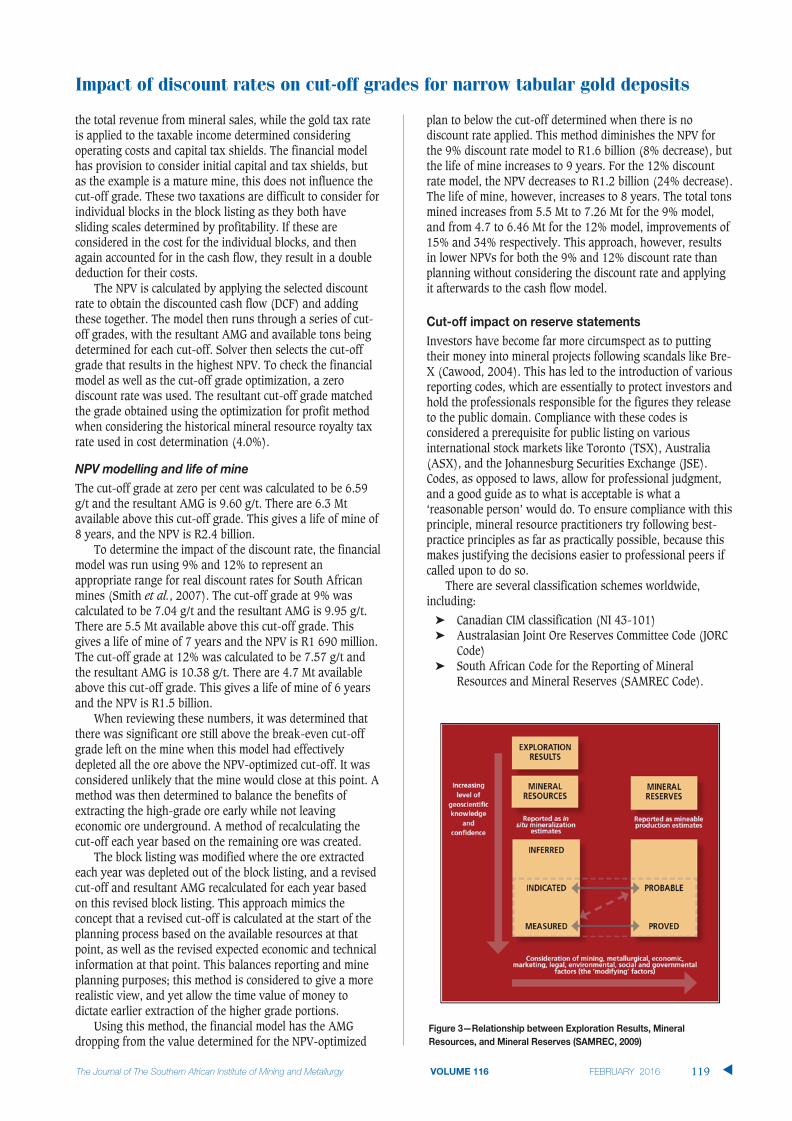
the total revenue from mineral sales, while the gold tax rateis applied to the taxable income determined consideringoperating costs and capital tax shields. The financial modelhas provision to consider initial capital and tax shields, butas the example is a mature mine, this does not influence thecut-off grade. These two taxations are difficult to consider forindividual blocks in the block listing as they both havesliding scales determined by profitability. If these areconsidered in the cost for the individual blocks, and thenagain accounted for in the cash flow, they result in a doublededuction for their costs.
The NPV is calculated by applying the selected discountrate to obtain the discounted cash flow (DCF) and addingthese together. The model then runs through a series of cut-off grades, with the resultant AMG and available tons beingdetermined for each cut-off. Solver then selects the cut-offgrade that results in the highest NPV. To check the financialmodel as well as the cut-off grade optimization, a zerodiscount rate was used. The resultant cut-off grade matchedthe grade obtained using the optimization for profit methodwhen considering the historical mineral resource royalty taxrate used in cost determination (4.0%).
The cut-off grade at zero per cent was calculated to be 6.59g/t and the resultant AMG is 9.60 g/t. There are 6.3 Mtavailable above this cut-off grade. This gives a life of mine of8 years, and the NPV is R2.4 billion.
To determine the impact of the discount rate, the financialmodel was run using 9% and 12% to represent anappropriate range for real discount rates for South Africanmines (Smith et al., 2007). The cut-off grade at 9% wascalculated to be 7.04 g/t and the resultant AMG is 9.95 g/t.There are 5.5 Mt available above this cut-off grade. Thisgives a life of mine of 7 years and the NPV is R1 690 million.The cut-off grade at 12% was calculated to be 7.57 g/t andthe resultant AMG is 10.38 g/t. There are 4.7 Mt availableabove this cut-off grade. This gives a life of mine of 6 yearsand the NPV is R1.5 billion.
When reviewing these numbers, it was determined thatthere was significant ore still above the break-even cut-offgrade left on the mine when this model had effectivelydepleted all the ore above the NPV-optimized cut-off. It wasconsidered unlikely that the mine would close at this point. Amethod was then determined to balance the benefits ofextracting the high-grade ore early while not leavingeconomic ore underground. A method of recalculating thecut-off each year based on the remaining ore was created.
The block listing was modified where the ore extractedeach year was depleted out of the block listing, and a revisedcut-off and resultant AMG recalculated for each year basedon this revised block listing. This approach mimics theconcept that a revised cut-off is calculated at the start of theplanning process based on the available resources at thatpoint, as well as the revised expected economic and technicalinformation at that point. This balances reporting and mineplanning purposes; this method is considered to give a morerealistic view, and yet allow the time value of money todictate earlier extraction of the higher grade portions.
Using this method, the financial model has the AMGdropping from the value determined for the NPV-optimized
plan to below the cut-off determined when there is nodiscount rate applied. This method diminishes the NPV forthe 9% discount rate model to R1.6 billion (8% decrease), butthe life of mine increases to 9 years. For the 12% discountrate model, the NPV decreases to R1.2 billion (24% decrease).The life of mine, however, increases to 8 years. The total tonsmined increases from 5.5 Mt to 7.26 Mt for the 9% model,and from 4.7 to 6.46 Mt for the 12% model, improvements of15% and 34% respectively. This approach, however, resultsin lower NPVs for both the 9% and 12% discount rate thanplanning without considering the discount rate and applyingit afterwards to the cash flow model.
Investors have become far more circumspect as to puttingtheir money into mineral projects following scandals like Bre-X (Cawood, 2004). This has led to the introduction of variousreporting codes, which are essentially to protect investors andhold the professionals responsible for the figures they releaseto the public domain. Compliance with these codes isconsidered a prerequisite for public listing on variousinternational stock markets like Toronto (TSX), Australia(ASX), and the Johannesburg Securities Exchange (JSE).Codes, as opposed to laws, allow for professional judgment,and a good guide as to what is acceptable is what a‘reasonable person’ would do. To ensure compliance with thisprinciple, mineral resource practitioners try following best-practice principles as far as practically possible, because thismakes justifying the decisions easier to professional peers ifcalled upon to do so.
There are several classification schemes worldwide,including:
� Canadian CIM classification (NI 43-101)� Australasian Joint Ore Reserves Committee Code (JORC
Code) � South African Code for the Reporting of Mineral
Resources and Mineral Reserves (SAMREC Code).
Impact of discount rates on cut-off grades for narrow tabular gold deposits
VOLUME 116 119 �

Impact of discount rates on cut-off grades for narrow tabular gold deposits
For this paper, the SAMREC Code has been used forillustration purposes, but the other codes share the samedefinitions and broadly follow the same requirements forcompliance. Figure 3 shows the relationship between mineraloccurrences, Inferred, Indicated, and Measured resources, aswell as the modifying factors required to convert Resourcesinto Reserves.
To comply with the SAMREC Code regarding thedeclaration of resources and reserves, various aspects need tobe recorded and documented in a series of tables. Table I isan extract from SAMREC Code Table 5.7, which deals witheconomic criteria when regarding Exploration Results,Mineral Resources, and Mineral Reserves.
As can be seen in the table, the SAMREC Code has nospecific requirement to disclose the WACC, and thus whatwould be considered an appropriate discount rate for themining company. Different companies have different WACCsdue to how they structure their debt/equity (debt is generallyconsidered cheaper than equity), as well as how risky theyconsider the project. There is, however, a requirement to’State, describe and justify all economic criteria that havebeen used for the study’, including those used to determinecut-off grades. In Mineral Reserves (ii, iii, and v), itfurthermore states that applicable taxes and royaltyallowances should also be considered in how the cut-offgrade is calculated.
Cut-off grades are used for two primary purposes: todeclare a Mineral Reserve from a Mineral Resource, and formine planning. There should be no conflict arising betweenthese two objectives. Companies will always try and increasethe amount of Mineral Reserve they declare, becauseinvestors place value on this. By having a lower cut-offgrade, the Mineral Reserve will automatically increase asmore of the Mineral Resource will be above this grade, andthus become part of the Mineral Reserve. Using a cut-offgrade that just considers overall profit or break-even ignores
the currently accepted measure of financial value which is theNPV. The cost of capital should also be considered in determining the cut-off grade. The time value of money andfocusing on NPV rather than just overall profit means that thehigher grade portions of the orebody should be mined first.Using this resultant higher grade cut-off grade only,however, leads to a lower overall extraction of the orebody,and economic portions above the break-even grade areeffectively abandoned. When valuing an orebody using theDCF method, the SAMVAL Code requires a full disclosure ofthe WACC as well as how the discount rate being applied wasobtained (SAMVAL, 2009).
Table II shows the overall measured and indicatedresource for the mine analysed for this study. Table III showsthe summary of Mineral Reserves (Proven and Probable) thatwould result by applying the different cut-off grade strategiesdiscussed.
For this summary, the various methods for calculating thecut-off grade have been tabulated indicating the cut-offgrade, total tons milled (including dilutions and plannedwaste), life of reserve, resultant AMG, recovery grade(including PRF), recovered ounces, and the profit or NPV. Forthe methods where the profit was calculated, this wasdiscounted using either 9% or 12% to allow directcomparison with the methods that were optimized at thesetwo rates. All the methods utilized the same final cash flow
�
120 VOLUME 116
Table I
SAMREC Code Table 5.7. Economic criteria for Exploration Results, Resources, and Reserves (SAMREC, 2009)
Exploration Results (A) Mineral Resources (B) Mineral Reserves(C)
(i) Not usually reported. (i) In reporting, a Mineral Resource should (i) For Mineral Reserves, parameters should be detailed withIf mentioned, however, factors meet the minimum requirement of engineering completed to a pre-feasibility study engineering significant to project economics ‘reasonable prospects for eventual completed to a pre-feasibility study level as defined in the should be current and based on economic extraction’ SAMREC code.generally accepted industry practice (ii) State and define the reasonable and realistic (ii) State, describe and justify all economic criteria that have beenand experience. Assumptions should assumptions/parameters (albeit preliminary, e.g. used for the study such as capital and operating costs, exchange be clearly defined. cut-off grade, cut-off screen size, product price or rates, revenue / price curves, royalties, cut-off grades, reserve
other criteria) used to assess eventual likelihood pay limits.of economic extraction. (iii) Summary description of method used to estimate the (iii) These assumptions and factors should be commodity price profiles used for cut-off grade calculation, reasonably developed and based on generally economic analysis and project valuation, including applicableaccepted industry practice and experience. taxes, inflation indices and exchange rates.If appropriate, state the level of study. (iv) Demonstrate that the product price assumptions are
reasonable and supportable. Justify assumptions made concerning production cost and value of product. Consider transportation, treatment, penalties, exchange rates, marketing and other costs.(v) Allowances should be made for royalties’ payable, both to government and private.(vi) Resource/Reserve sensitivity – detailed description of method used and results obtained.
Table II
Total Measured and Indicated Resource (cut-off 0 g/t)
Classification Mt Grade (g/t) Content (million ounces)
Measured and Indicated 14.0 3.71 1.67

model to determine the final profit/NPV. This cash flowincluded the expected PRF, dilutions and planned waste,mineral resource royalty tax, and income tax based on thegold tax formula. All cash flow models utilized the samecommodity price, exchange rate, fixed cost, variable cost, andproduction rate.
As can be observed, the NPV optimized at 0% resulted inthe highest profit. However, when the actual cost of capitaland the timing of the extraction are considered, this type ofcut-off grade determination results in an overall lower NPV.When optimization purely on NPV occurs, the focus is on thehighest grade portion of the orebody initially. This results ina shorter life of mine and lower overall orebody utilization.With this type of approach, the model indicates the orebodyis depleted when significant resources still remainunderground that could be economically extracted.
The models where the cut-off grade and resultant AMGwere recalculated each year (as the orebody was depletedwith the approach to maximize the NPV of the remaining ore)were not satisfactory. The life of mine remained the same orhigher than when optimizing with the view of maximumprofit (0% model with NPV at zero), but the AMG quicklydrops as the higher grade portions are depleted initially.While the mine remains profitable for a longer period, theNPV is severely diminished compared to the models wherethe NPV at 9% and 12% are the prime focus.
The impact of the varying the discount rate on the cut-offgrade and NPV is displayed in Figure 4.
The relationship between cut-off grade and the discountrate is not a smooth curve, but has distinctive step changes.This is a function of the model used and the particular blocklisting. Different orebody block listings will display thisrelationship in different forms, depending on the number ofblocks and where the peak for optimization occurs for eachrun of the optimization model as it is selecting a specificblock value. The relationship between the discount rate andNPV can be approximated with a smooth polynomial polylineand is a function of the amount of ore mined, the life of mine,as well as the degree of discounting of the resultant cashflow.
The cost of capital and the concept of time value of moneyhave a significant impact on cut-off grades if modelled to
maximize NPV. The current trend is to focus on value, andnot just overall profit. This has resulted on companiesoptimizing regarding the DCF and resultant NPV as theprimary measure of value. The investors are, however, notthe only stakeholders in a mining business. Dueconsideration should be given to employees, the communityin which a mine operates, as well as the State. Thjeoverriding concern of these would be for a long life of mineas well as maximum exploitation of the orebody.
Cut-off grades can be determined in a number of ways.These range from simple break-even calculations to verycomplex models considering multiple facets of the miningbusiness, including the effects of variations in the miningenvironment (Smith et al., 2007). In this study, however, theorebody, ore flow, as well as the cash flow, are the primefocus areas of consideration in determining optimal cut-offgrade. A simple Microsoft Excel cut-off grade modelling toolhas been developed that links the block listing, ore flow, andcash flow, and uses the Solver optimization tool. The impactof both the mineral resource royalty tax, as well as theincome tax, is considered in determining the optimal cut-offgrade. The SAMREC Code requires the cost of taxation to beincluded in the economic analysis in determining what theeconomically extractable portion of the mineral resource is.
Impact of discount rates on cut-off grades for narrow tabular gold deposits
VOLUME 116 121 �
Table III
Proven and Probable Reserves calculated using different methods
Description Cut-off Tons milled Life of AMG Rec. grade Rec. ounces Profit 0% NPV @ 9% NPV @ 12%grade (g/t) (millions) reserve (g/t) (g/t) (millions) (millions) (millions) (millions)
Basic break-even 5.25 9.69 12 8.39 4.41 1.37 R2 034 R1 258 R1 098
Break-even, No royalty 6.17 7.26 9 9.26 4.80 1.12 R2 316 R1 564 R1 395
Break-even, 3% royalty 6.54 6.45 8 9.56 5.03 1.04 R2 386 R1 651 R1 482
Break-even, 5% royalty 6.63 6.45 8 9.63 4.94 1.03 R2 262 R1 598 R1 442
NPV-optimized, 0% discount 6.56 6.45 8 9.57 5.03 1.04 R2 394 R1 659 R1 489
NPV-optimized, 9% discount 7.04 5.50 7 9.95 5.37 0.95 - R1 690 -
NPV optimized, 12% discount 7.57 4.84 6 10.38 5.45 0.85 - - R1 548
NPV -optimized, variable cut-off 9% 5.68-7.61 7.26 9 8.79-10.41 4.77 1.12 - R1 557 -
NPV optimized, variable cut-off 12% 4.20-7.61 6.45 8 7.77- 10.41 4.58 0.95 - - R1 181

Impact of discount rates on cut-off grades for narrow tabular gold deposits
The concept of variation has been ignored as it adds awhole level of complexity, requiring tools like Monte Carlosimulation to address. As these tools are not part of the basicMicrosoft Excel package, they are considered beyond thescope of this paper. The orebody considered in this study is amature South African gold deposit, and it is assumed that allthe initial capital included in the tax shield has been depleted.As a result of there being no negative cash flow in the initialyears (capital payback), no IRR could be determined for thevarious model options. Ongoing capital costs are included inthe working costs for simplicity of determining the break-even cut-off grades. When using the NPV-optimizedmethods, splitting the ongoing capital from the working costscould have benefits in how the taxation is calculated. Thiswould differ for each mining company, according to how theyconsider their capital structure.
It has been shown that determining cut-off grades with amethod that does not take the cost of capital and discountrate into the calculation results in lower NPVs when adiscount rate is later applied. It has also been shown thatoptimizing on NPV alone results in partial extraction ofeconomic ore, and thus lower mineral reserve value.Investors place value on the mineral reserve statement, andlower quantities of economic ore could negatively impact amining company’s investment potential.
Lane (1988) considered how to optimize extraction in theearly years of a project to ensure early capital payback, andstill get high total ore extraction. He determined differentmethods to calculate the cut-off grade at different points in amine’s value cycle. He proposed using a budget cut-off in theearly years where the cost of capital is added onto the profit,then an optimal cut-off grade through the bulk of the projectlife. When the available ore dropped to the point that the millwas not running at its maximum capacity, Lane proposedcalculating a marginal cut-off grade to extract the ore thathad been left previously. In determining the marginal cut-offgrade, he proposed removing development costs as well asmilling costs, as this ore would have been accessed earlier inthe mine’s life, and the mill is the most economical whenrunning at its maximum capacity. The spare capacity in themill could be filled, with no additional milling costs, with oreabove the marginal cut-off grade. This would contributeeconomically, as controlling the total unit cost is critical inensuring the cut-off grade is valid (Lane, 1988). In theexample presented as part of this study, the marginal cut-offgrade concept has not been applied, but there would besignificant material above this grade. Using a variable cut-offgrade strategy as proposed in this study would replace theneed to determine a budget cut-off, as this is automaticallydetermined in the model.
Block listings are dynamic. This cut-off grade has beendetermined at a point in time to direct mine planningprimarily for the following 12 months, and guide longer termplanning. It also reflects the remaining ore available on themine, as well as the geological confidence in the orebody atthat point in time. As the mine continues to develop andconduct further exploration, Inferred mineral resources will
be upgraded to Indicated or Measured mineral resources, andpotentially become part of the Mineral Reserve. Consideringthis, the published Mineral Reserve can never be consideredthe final amount of ore that will be mined until just prior tomine closure.
Optimizing the cut-off grade with the view of maximizingprofit (0% NPV) gives the best balance regarding life of mine,overall tons, and profit. Optimizing using the NPV as the keydriver reduces life of mine significantly, for a small benefit inthe NPV at both 9% and 12% (2% and 4% respectively). TheSAMREC Code does not require a specific statement to bemade regarding the cost of capital and subsequent discountrate. The impact of applying the discount rate into the cashflow model on the total declarable reserve ounces issignificant if using the NPV as the optimizer driver. Thisimpact was found to be 9% and 19% for the 9% and 12%discount rates respectively.
Using cut-off grades as a primary planning tool is verysimplistic. It assumes that the production levels will bemaintained at the optimal level. The grade distribution in theorebody is not considered, nor what ore is available forimmediate extraction. The resultant ore flow used ingenerating the cash flow (and the resultant DCF to calculateNPV and IRR) assumes the AMG will be maintainedconstantly.
CAWOOD, F.T. 2004. Towards a mineral property valuation. Journal of the South
African Institute of Mining and Metallurgy, vol. 104, no. 1. pp. 35–43.
CORREIA, C., FLYNN, D., ULIANA, E., and WORMALD, M. 2013. Financial
Management. 7th edn. Juta, Cape Town.
LANE, K.F. 1988. The Economic Definition of Ore. Mining Journal Books,
London.
MEISSNER, J. and NGUYEN, T. 2014. An Introduction to Spreadsheet Optimization
Using Excel Solver. Meiss Research Group.
http://www.meiss.com/download/Spreadsheet-Optimization-Solver.pdf
[Accessed 2/12/2014].
SAMREC. 2009. South African Mineral Resource Committee. The South African
Code for Reporting of Exploration Results, Mineral Resources and Mineral
Reserves (the SAMREC Code). 2007 Edition as amended July 2009.
http://www.samcode.co.za/downloads/SAMREC2009.pdf [Accessed 10
April 2014].
SAMVAL. 2009. South African Mineral Asset Valuation (SAMVAL) Working
Group. The South African Code for the Reporting of Mineral Asset
Valuation (The SAMVAL Code). 2008 Edition as amended July 2009.
http://www.samcode.co.za/downloads/SAMVAL2009.pdf [Accessed 1
December 2014].
SMITH, G.L., PEARSON-TAYLOR, J., ANDERSON, D.C., and MARSH, A.M., 2007. Project
valuation, capital investment and strategic alignment—tools and
techniques at Anglo Platinum. Journal of the Southern African Institute of
Mining and Metallurgy, vol. 107. pp. 67–74. �
�
122 VOLUME 116

Mine operators and engineers are compelled toreview the way they look at projects due tochanging mining conditions, legislative issues,rising electricity costs, and the constrainedsupply of skills in South Africa.
Pre-feasibility studies and valuationmethodologies to assess such impacts arebecoming increasingly important. For example,in a hard-rock mining operation, cost control isapplied by reducing blasting. However, thisincreases the overall cost of the operation,because poorly fragmented ore increasesmaterial handling demands. There is a
decreased throughput due to damage toconveyors and transfer chutes, or poor skiputilization. Ultimately, milling costs increasesubstantially.
The inclusion of the long-term effects onindirect stakeholders and mercurial policieshave also been overlooked in performancestudies. The quantification of social andenvironmental risks/benefits for allstakeholders at the end of the life of project(LOP) have been influencing the way in whichdecisions are made. Life-cycle activities(cradle-to-grave), beyond the boundaries ofthe operation, can no longer be omitted. Whenthese are disregarded, the project undergoesmultiple iterations leading to semi-optimaloperation.
Hence, there is an increased focus onperformance realization for sustainability, andcash flows are starting to incorporate theeconomics pertaining to the externalenvironment. These costs are labelled externalbecause they are not directly accounted for inproduction output rates.
Therefore, to understand and encompassthe real value of a project or operation, re-selecting KPIs (originally identified in a basecase) to support the overall performance of theoperation has become a necessity.
Business optimization (BO) adopts method-ologies to select the best alternatives tosimultaneously increase the benefits andreduce the risks. It is conducted across themining value chain activities of a depleting
Business optimization for platinummining projects and operationsby P.J. Petit*
The complex planning required to achieve any planned production yieldsmultiple and dissociated responses over the life of project (LOP). Thecustomary decision-making process negates the possibilities of developingoptimized and integral solutions from operating levels up to business andstrategic levels. This results in an inefficient project or overall underper-formance of the operation.
In the project setting, disconnected trade-offs and improvedperformance studies become inadequate, because they are site-specific anduse only a few comparative parameters. They are often based on a smalldata-set.
Decisions taken to achieve overall objectives require the correctdetermination and dissemination of key performance indicators (KPIs).The KPIs indicate efficiency in operation, whereby the marginal rate oftechnical substitution corresponds to the rate of production. It is thenecessary condition for optimization. Performance realization for sustain-ability follows optimization modelling, the latter often being presentedwith financial results such as business net present value (NPV). Itconsiders techno-financial constraints and provides a strategic and alignedoutlook of KPI decisions for an enhanced and integrated outcome.
This paper explains a mining case study that is rendered efficient, andthrough business optimization (BO) short-term and sustainable targets arereached. Business optimization increases the NPV by 14.7%. This isachieved by challenging conventional decision-making associated withmaximizing business value by including environmental externalitieswithin the LOP.
business optimization, key performance indicators, valuation methodologies, multiple-criteria decision-making (MCDM), analyticalhierarchical process (AHP), environmental externalities.
* Independent Consultant.© The Southern African Institute of Mining and
Metallurgy, 2016. ISSN 2225-6253. This paperwas first presented at the, Mining BusinessOptimization Conference 2015, 11–12 March2015, Mintek, Randburg.
123VOLUME 116 �
http://dx.doi.org/10.17159/2411-9717/2016/v116n2a3

Business optimization for platinum mining projects and operations
resource. BO also aims to improve the financial outcomes ofthe business and to ensure long-term gains for allstakeholders.
In the literature, BO has focused primarily on mining andprocessing solutions. Without the impact that engineeringactivities can provide, improvements have been relative, andbottlenecks, mostly technical constraints, have been mostlyviewed in terms of a capital injection, instead of analternative engineering solution, with the potential foradditional or unforeseen benefits at minimal cost.
An increased concern for decreasing and deteriorating naturalresources has resulted in the environment being valued as anasset. This asset, external to the direct project outcomes,includes the atmosphere, water sources, and land. It is‘operationalized’ through explicit changes in its environ-mental status.
In this case study, environment externalities arise whenactivities or events of the mining producer have external(indirect) unintended beneficial or negative effects on otherproducers and/or consumers. Environmental externalitiesinclude:
� Residuals such as reject products, waste rock,discharge water, and air pollution
� Intangibles such as irreversible changes and environ-mental damage
� Incommensurables, including the effects of anactivity/event that are, with some effort, assignedmonetary value.
A basic evaluation matrix (BEM) can be used to optimize abase case and to cater for external objectives. Due to timeconstraints, the tendency is generally to revert to‘engineering judgement’ or previous experience, biasedtowards satisfying the perceived dominant parameter at thatpoint in time. This approach has several shortcomings.
� It is based on trade-off studies that are site-specific� Primary cost-related drivers are used, which are based
on a small data-set� Power and water studies omit ancillary usage and
reticulation possibilities.
No single parameter can be viewed in isolation, due to thedirect or indirect relationships that exist between parameters,as shown in Figure 1. The collection of data from otheroperations also has the capacity to provide insight into, orvalidate, parameters to potentially render themcertain/controllable.
Certainty depends on the information base and itsquantification, which can facilitate decision-making.Controllable parameters allow decisions to be easilyenumerated, unlike parameters susceptible to externalities.An increase in uncertainty across parameters, with fluctu-ations between the extremes of control, makes decision-making complex and results in multiple outcomes(scenarios).
The parameters in Figure 1 were assigned realistic andnumeric ratings for the base case. This revealed inefficienciesand resulted in the implementation of alternative engineeringsolutions. The exercise was repeated to render the base caseefficient.
Subsequently, applying the principles of financialmechanics modelling, a comprehensive techno-financialmodel (TFM) was built. The TFM incorporates activity-basedcosting with some costing based on first-principles costingmethodology. Sensitivities, scenarios, and realistic riskprofiles were applied to simultaneously determine the impactof both technical and cost drivers, and their throughput effectat business level. This method has the potential to yieldunexpected KPIs.
KPIs that became prominent were power savings, thecapacity and the quality of the water source (the supply), thewater consumption rates and reticulation routes, and theinfluence of environmental taxes. These KPIs led a re-basedreference for design enhancement and operating initiativesthat could potentially lead to optimization.
The revised base case was then optimized to yield asolution that was holistic (with consideration of externalities)at operating, business, and strategic levels. With BO,engineering (non-mining) solutions were integrated toensure that non-process infrastructure, supporting services,and all throughput processes were considered.Environmental, social, and other legislative aspects wereencompassed in this iterative exercise such that each iterationtook into account the strengths, weaknesses, opportunities,and threats (SWOT) of the solutions generated.
Replacement cases, alternatives, and options wereintroduced and subject to decision-making techniques. Theresults were transferred to a business optimization matrix(BOM) of the project or operation.
The remainder of this paper illustrates the BO approachand the multiple-criteria decision-making process in a typicalproject.
The team, tasked with a greenfield platinum project with alife of project (LOP) of 13 years, wishes to optimize itsunderground mining methodology to firstly reduce power andsecondly, to lower its impact on an open water source.
�
124 VOLUME 116

Electricity consumption is to be kept to a minimum, duenot only to rising electricity prices, but also to constraints onallocation. In the case of water, the open source is utilized notonly by the mine, but also by the local community fordomestic consumption. Due to the semi-arid climate in thearea, the volume of the open water source is anticipated todiminish significantly over the LOP. Consequently, thenitrate-nitrogen concentration of the water supply and thenitrate load generated by the mine are to be considered.
The base case (Case 1) established on the reserve layoutwas generated by:
� Use of a traditional hard-rock tabular mining method,namely hand-held electric drilling with hydropowersupport, the latter as was practised at Bokoni andTwickenham platinum mines
� Omitting any consideration for environmentalexternalities by initially maintaining the open watersource at constant volume, with no seasonal fluctu-ations. The life-cycle monthly water extraction was alsokept constant In this instance; however, this allowedthe initial condition for inflow and outflow character-istics of nitrate concentration and nitrate amounts to beset.
� Neglecting de-nitrification� Disregarding the impending carbon tax� Omitting the impact of the underground engineering
footprint.
Subsequent to the establishment of the base case, the miningdesign was changed from a half-level approach to blockmining. A typical underground decline layout consists of adecline cluster feeding sub-levels of geometric consistency.The mine re-planning resulted in a decline cluster feeding ascheduled series of blocks, thus promoting access to highergrades of ore earlier on in the LOP. The lower value blocksare bypassed, and accessed later in the LOP. Although thiswas a substantial task for mine planning and scheduling, thisconsiderably reduced the mining footprint and developmentcosts. However, other challenges remained.
The production drilling equipment in the base case (Case1) was no longer viable in terms of real-time changes for theLOP. (The electrical equipment was assessed on a leaseagreement for the LOP). Alternative recognized and testeddrilling methods were proposed, as follows:
� Alternative case (Case 2): hydropower drilling withhydropower support, with an open-circuit system,powerpacks in the crosscut and high-pressure pipereticulation in the stope. The drills are driven by thewater, which is then discarded and pumped out of thestopes, as performed at Northam Platinum,Twickenham, Dwarsrivier, Karee, and Amandelbultmines
� Alternative case (Case 3): electric drilling with localizedcompressed air support – new alternative.
A multiple-criteria decision-making process known as the
analytical hierarchical process (AHP) was applied to selectthe mining technology. The AHP expresses the relativevalues of a set of criteria of different parametric units, withina matrix, to rank or eliminate cases by
� Listing of systematic and unsystematic criteria� Rating each criterion out of 10 in an inverse square
matrix� Including all project and production personnel.
The pertinent outcome, shown in Figure 2, was derivedby using a set of pairwise comparisons configured in theBEM. These comparisons were used to obtain the weights ofimportance (ranking) for the drilling technology decision, andthe relative performance measures of the alternatives, knownas relative values (RVs), in terms of each individual decisionparameter.
In Figure 2, the core of the graph represents 0% or lowestranking, and the greater the distance from the centre, thebetter the score, and thus the more preferable the solution asrepresented by the higher percentage.
In the AHP results, the penetration rate was the dominantparameter for the LOP. The penetration rate is sensitiveacross drilling methods, and it affects parameters such asenergy delivery to the rock face; water consumption; capitalexpenditure; safety, health, and environment (SHE); andtechnology phase change and its implementation. The above-mentioned parameters can be controlled, but they are affectedby other parameters, namely projected productionperformance, electricity cost, and legislation, the latter ofwhich cannot be controlled.
Variable penetration rates experienced at existingoperations are adverse to the production objectives for theLOP. Due to the variability of the rock conditions, and theoption to access the UG2 Reef at a later stage, consistency inthe penetration rates to achieve the production cycle wasimperative.
Electricity consumption also showed a significantvariability, based on the variability of drilling time per hole atthe stoping face, while operating costs were of lesser value in
Business optimization for platinum mining projects and operations
125VOLUME 116 �

Business optimization for platinum mining projects and operations
the AHP results. Electricity consumption was identified inview of the relation between energy consumption andgreenhouse gas (GHG) emissions and the proposed carbontax anticipated for introduction in July 2016.
Implementation complexity and specialist maintenanceacross the re-planned mining layout rendered the base casedrilling methodology unviable for the LOP under consid-eration in the project, as shown in Figure 2.
Legislative and SHE aspects pertaining to noise, oil, anddust generation were all satisfied in each case.
Low water consumption was a prerequisite in theselection of the base case and for the alternative cases.Subsequently, it formed part of electricity consumption sincewater requires energy to reach the mining blocks and waterreticulation affects implementation. It was noted that lowwater consumption at the mine contributes to communitybenefits, and indirectly to creating a micro-economic zone forcommunity-generated income in the vicinity of the project.
The AHP results for stoping indicated that the preferredoption was hydropower drilling with hydropower support(Case 2), mainly because of consistent penetration ratesexperienced at existing operations and test results across rockconditions. Reduced labour requirements with betterpenetration rates were an operating cost consideration.Subsequently, this permits for the up-skilling of rock drilloperators (RDOs) and engineering crews.
In addition, since the mine plan has been de-constrainedfrom half-levels to mining blocks, the modular configurationof the hydropower solution eases relocation of equipment. Aclosed-circuit water reticulation system is also possible whenremote blocks are drilled far from the decline cluster.
Hydropower drilling with hydropower support was alsodeemed advantageous for short-term planning in the event ofunforeseen events (geotechnical), and for long-term planningif mining of the UG2 Reef is later considered.
Electric drilling with localized compressed air support(Case 3) was discarded from a technical perspective. Multiplecompressors stationed at simultaneously mined blocksaggregated to higher electricity consumption andmaintenance requirements than a surface compressorunit/station. Independent supply of air from surface to refugechambers in the mining blocks was also a technical and costconstraint. The extent of compressed air delivery to theremotely mined blocks will still be subject to pipe leakages.
Strategic project planning, based solely on the perceivedprimary parameter, namely capital, did not offer the mostadvantageous solution. Although the NPV confirms thetechnical decision in Table I, namely Case 2, if the capex andopex were the only parameters considered for the decision,Case 2 would not have been selected. Hence, viewing thesefinancial parameters collectively yielded a counterintuitiveoutcome, and contradicted the selection of the original KPIs.The business NPV and the peak funding requirements alsoconfirm the techno-financial decision.
The selection of the stoping method cannot be confined towithin the boundaries of the operation. In this project, anincreased concern for decreasing raw water availability anddeterioration of water quality has led to water being‘operationalized’.
Environmental externalities arise when activities ofproducers, or consumers, have external (indirect) unintendedbeneficial or negative effects on other producers or/andconsumers. Negative inter-temporal externalities occur whenexhaustible resources are depleted. Therefore, the movementof water was ‘operationalized’ from source to sink.
In this case study, the open water source is subject towater pollution, irreversible changes, and environmentaldamage. The mine discharges minewater with a nitratecontent into a simultaneous water source and sink. Allconsumers of this polluted water incur rising costs of treatingwater for consumption, and within the operation, increasingproduction costs and secondary operating costs occur, suchas health claims, and other private- and social-related costs.
Prior to costing denitrification solutions, the project teamtook measurements of the pre-project nitrate concentration.The pre-project capacity of the open water source wasapproximately 28 000 M . The laboratory results indicatedelevated nitrate concentrations at 35.0 g/M . The SANSnitrate concentration allowance for the project as per SANSClass 1 is 10.0 g/M
The natural increase in nitrate concentration in the openwater source at the end of LOP, for a reduced water sourcevolume is projected at 39.4 g/M . Over and above thisrealization, the mine planned to discharge 4 M of water permonth with a nitrate concentration of 75.0 g/M .
�
126 VOLUME 116
Table I
Financial valuation results of stoping selection (real terms)
Platinum operation 94 kt/month, 13 years LOP Base Case Case 2 Case 3
Direct operating cost (excl. contractor labour) ZAR million 856 993 626
Contractor mining labour ZAR million 11.51 8.87 11.53
Direct operating cost rate ZAR/tROM 764.87 609.67 751.76
Direct capital cost (excl. contingency) ZAR million 949 1.837 852
NPV post-tax @ 10% discount ZAR million 7 530 8 533 7 644
Internal rate of return (total project) percent 10.67% 11.24% 10.73%
Business NPV ZAR/tROM 469.33 531.82 476.44
Peak funding requirement ZAR million 87 78 83

Regulatory mechanisms are enforceable on the miningcompany. Penalties are implementable if the nitrate concen-tration/threshold in this common-property resource reaches38.0 g/M during the LOP. The pollution charge is a functionof the concentrations of pollutants above this prescribed limit.Hence, measures to reduce the reliance on the open waterresource and reduce the nitrate load in the discharge wastewater were imperative. The impact on the overall projectcapital estimate was also to be limited.
A water balance of the open water source over the LOP wasdeveloped, and included on-site water recycling activities andrecirculation flows. In the majority of projects, the waterbalance usually focuses on internal water movement andstorage capacities, but excludes the impacts on the externalsupply (the open water source).
Once the comprehensive water balance was completed,the water pollution in the BAU base scenario (do-nothingscenario) was generated by initially maintaining the openwater source at constant volume (no fluctuations). Thisallowed the initial condition for inflow and outflow character-istics of nitrate concentration and nitrate amounts to be set.The capacity of the open water source was then fluctuatedmonthly over the LOP. An assumption was made that waterwas mixed uniformly over a fluctuating open water sourcevolume. Thereafter, a climatic change (successive series ofdry seasons) was inserted in the last six years of the LOP.The LOP water extraction was kept constant at 36 M /month.
With these conditions, the monthly nitrate concentrationof the open water source, volume inflows (replenishment),and outflows (depletion) were calculated over the LOP byusing transcendental calculations (non-algebraic functions).In this project, the pollution was generated from astationary/point source, the underground mine.
The completion of the BAU base case provided theopportunity to generate water- and energy efficient
possibilities. The mining activity, water consumption, anddischarge by the operation have direct and indirectconsequences on project capitalization. The incentive existedto abate the release of pollution by introducing cost-effectivedenitrification technologies.
Several denitrification processes were investigated. Basedon the design criteria of the project, reverse osmosis (RO)was deemed the most suitable to treat high-nitrate water forthe LOP and to ensure compliance with regulatory nitrateconcentration levels. Additional benefits include effectivedesalination with comparatively moderate operating costs.
Denitrification allows for containment, recycling, andrecirculation of water on-site, and therefore the successivereduction of demand from the open water source. Thiseliminated cost penalties incurred due to accidental dischargeof untreated water into the open water source.
Initial capital requirements were also curtailed becausepiping and pumping requirements from the open water sourcewere scaled down, and continuous recirculation of waterwithin the operation reduced the size of the water storagefacilities (smaller footprint). Hence, the financial capitalprerequisite was controlled because it will be easier torehabilitate a smaller volume of water during the course ofthe operation, resulting in faster closure.
Actively mitigating the risk of the projected nitrateconcentration in the open water source controlled the effecton natural capital, social capital, on-site capital requirements,and financial capital prerequisites.
The nitrate treatment using RO was calculated for threescenarios as follows:
� Scenario 1—treatment of the water inflow into the openwater source only (water volume discharged by mine)
� Scenario 2—treatment of water outflow from the openwater source (water volume withdrawn by mine)
� Scenario 3—continuous treatment of water outflowfrom the open water source (continuous water volumewithdrawn by mine).
Business optimization for platinum mining projects and operations
VOLUME 116 127 �

Business optimization for platinum mining projects and operations
The short- and long-term effects of the water treatmentscenarios were calculated based on the monthly rates ofdepletion, dispersion/concentration/dilution, and replen-ishment, as well as the treatment investment costs per unitvolume over the LOP.
The change in the nitrate concentration in the open watersource for the BAU base case and the three treatmentscenarios is shown in Figure 3. The effect of climate changein the last six years is shown by the decreased volumes.
In the BAU base case, the initial nitrate concentration in the open water source was 35.0 g/M . It increased to 39.4 g/M by the end of LOP as a result of the reduced damvolume (see previous section entitled Effect of the miningoperation on a natural resource for further details). Thus, thesmaller open water source volume towards the end of LOPhas a significant impact on the water quality.
In Scenario 1, the nitrate concentration in the treatedinflow (water discharged from mine) is 37.7 g/M with theimplementation of a two-unit 5000 /h RO plant at the start ofthe project. The RO plant processes water from the operationuntil the project is self-contained.
The limitations of the ten-unit 5000 /h reverse osmosisplant installed at the start of the LOP in Scenario 2 constrainthe nitrate removal to a 36.0 M /month throughput.Consequently, the process results in an open water sourceconcentration of 38.8 g/M at the end of LOP. It is noted thatthis is above the regulatory limit of 38.0 g/M . Hence, thisscenario is unsuitable.
In Scenario 3, the ten-unit 5000 /h RO plant is installedat the start of the LOP. Another three ten-unit 5000 /h ROplants were phased-in every three years. This improved theresult from Scenario 2, but it was insufficient to meet theimposed regulatory limit. At the end of LOP, the open watersource concentration is 38.2 g/M .
The increasing fluctuation of the nitrate concentration asthe project progresses shows the sensitivity to the volume ofthe open water source. It is noted that prior to the reducedopen water source volume (prior to the climatic change), thenitrate concentrations in Scenarios 1 and 3 meet, or werewithin reach of, the regulatory value of 38.0 g/M . Thesudden reduction in the open water source capacity indicatesthe sensitivity of nitrate-moderating capacity of the openwater source to its volume. This is an uncontrolled factor inthis case study.
Consequently, the Scenario 1 solution was selected.
An analysis of all emission sources in this project wasconducted. The carbon tax was calculated by aggregating theelectricity consumption of the mining and engineering
equipment used for the production cycle. An emissionconversion factor was applied to determine the carbonequivalents.
The South African government has proposed a carbon taxof R120 per ton CO2e on Scope 1 emissions. 1 kg of CO2 isemitted for every kilowatt-hour of energy produced andconsumed in South Africa. The tax will come into effect on 1July 2016, and increase by 10% a year. It is anticipated that60% of emissions will be tax-exempt for certain industries,and this threshold will apply in the first 5-year phase. Theeffective carbon tax ranges from R24.00 in 2016 to R35.14per ton CO2e from 2020 onwards. Table II quantifies the effectof the carbon tax estimation on the NPV for each scenario.
Interestingly, although Scenario 1 was selected based onthe denitrification assessment, should Scenario 3 have beenselected, a rebate would occur in the form of carbon offsets.This could be quantified in a trade-off study when clarity isobtained on the state of carbon trading and the South Africancarbon market. The capital investment and the penalty ofexceeding the regulatory limit of 38.0 g/M by 0.2 g/M versusthe carbon rebate potential will be valued in the future.
Subsequent to the denitrification assessment, theunderground mining and engineering water consumption andstorage were considered as follows:
� Option 1—series of cascade dams per mining blockestablished in the base case
� Option 2—open-ended feed from surface to a pressurebreak dam at the first production block. Fewer cascadedams, but with increased capacity, supplying multiple blocks are developed and pressure reducing stations(PRSs) are installed during block development,depending on the block mining scheduled and waterrequirements.
In the techno-financial analysis, Option 2 was selected.This option allowed for a smaller operating footprint and agreater flexibility for water storage. Piping and pumprequirements could be minimized through salvage and re-use.
The compounded decisions made for this project, using theBAU base case as a reference, yielded results that incorporatetechnical and financial considerations on parameters thataffect the open water source. In Table III, the BAU base case
�
128 VOLUME 116
Table II
Carbon tax estimation for each scenario
Platinum operation 94 kt/month, 13 years LOP Base Case Scenario 1 Scenario 2 Scenario 3
Carbon tax effect on NPV ZAR million - 2.76 2.40 (3.65)

with the selected mining technology is shown in the thirdcolumn. The results, based on the three RO nitrate treatmentscenarios, are progressed with the inclusion of the effect ofthe carbon tax, and then the selected underground waterdelivery storage and distribution system (Option 2).
The marginal cost of operating the RO plant was neutral,as compared to the BAU base case, hence proving that it isalso a cost-effective solution across the scenarios. Theoperating costs included reagents, power, and maintenance.Small changes in nitrate concentration affect the relativetreatment costs of delivering water for operations and denitri-fication. It tipped the financial case in favour of Scenario 1and highlighted the importance of reducing the dependenceof the open water source with the associated incoming waternitrate concentration (key driver).
Furthermore, this positive financial outcome offered thepotential to improve and capitalize water storage and distri-bution for the block mining layout. This is a function of thehigher risk profile when access to the open water source isrestricted due to drought conditions, and it is also to beconsidered if the UG2 Reef is mined in the future.
The business NPV is marginally better for Scenario 1 thanthe other scenarios. Although the difference is moderatesubsequent to the mining technology selection, the inclusionof the denitrification, carbon taxation, and the undergroundwater delivery, storage, and distribution system are based onthe effect the mining operation has on the open water source,and the requirement for the mining company to limit itsimpact on the deterioration of the open water source and topromote sustainability. This was achieved by re-selecting theKPIs to include environmental externalities and to supportthe overall performance of the operation over the LOP.
The context of such decisions was critical to the outcomeof the BO process and project value contribution, as shown inFigure 4. An increase in NPV of 14.7% for successive andconsolidated business enhancement was achieved for thiscase study.
It is not suggested that the solutions provided for thiscase study are applicable to variety of projects. However, it islikely that the results of the decision-making and valuationprocesses that took into account environmental externalitieswill be different from a process that is solely focused onproject or operating cash flow comparisons.
In BO, the aim is to apply the best technical solutions toensure that the production performance forecast prior toexecution is achieved, and that no technical constraintsinfluence the economic effect of the capital expenditure. Thisis because the financial and manufactured capitals are not theonly capital aspects of the project or operation.
Within the Six Capitals framework, other capital itemswere actively addressed. The natural capital, namely the openwater source, was stress-tested in terms of water volume andnitrate concentration. The reduced underground footprint wasa result of block mining and an optimized underground waterdelivery, storage, and distribution system. It contributed toreducing the impact on the natural capital by creating apositive control, which in turn impacts on the social andrelationship capital.
The implementation of a hydropower-based drillingmethod and the RO plant allowed for skills development andtraining, and cross-disciplinary opportunities for sustainableperformance through product and equipment improvement.Thus intellectual and human capitals were satisfied.
The integrated opportunities from the Six Capitalsframework improved the sustainable development (SD)performance.
This paper examined the effects of the need to incorporate BOfor projects and operations, in view of growing concernspertaining to the environment and climate change, andmicro-economic factors such as labour and skills shortages.
BO should be done in a systematic, integrated, andrigorous manner, as early as possible in the project life cycleto:
� Identify SWOTs and initiatives to enhance SHEQ andCSI
� Analyse cases, scenarios, and options against areference (BAU base case)
� Rank and prioritize by measuring effectiveness� Implement an action plan though decision-making � Obtain support for the decisions made.
Business optimization for platinum mining projects and operations
VOLUME 116 129 �
Table III
Financial valuation results of business optimization approach and the multiple-criteria decision-making process(real terms)
Platinum operation 94 kt/month, 13 years LOP Base Case Scenario 1 Scenario 2 Scenario 3
Direc.25t operating cost with RO ZAR '000 993 194 993 195 993 210 993 236
Operating cost rate of RO ZAR/tROM 7.41 7.41 7.41 7.41
Direct capital cost of RO ZAR million - 1 929 1 933 1 945
NPV post-tax @ 10% discount ZAR million 8 532.85 8 532.59 8 529.79 8 524.68
Internal rate of return percent 11.24% 11.23% 11.10% 11.10%
Carbon tax effect on NPV ZAR million - 2.76 2.40 (3.65)
NPV post-tax @ 10% discount (incl. PRS and cascade dams) ZAR million 8 532.85 8 641.45 8 638.65 8633.53
Business NPV ZAR/tROM 531.82 538.59 538.42 538.10

Business optimization for platinum mining projects and operations
BO is accomplished with committed implementation of thestrategies that can be controlled and evaluated againstrelevant KPIs.
The author would like to acknowledge the contributions fromHilti, Hydro Power Equipment, Novatek, Anglo Platinum, andBRPM operations, and Platinum Group Metals Limited forfacilitating access to study data.
ATAEL, M., JAMSHIDI, M., SERESHIKI, F., and JALALI, S.M.E. 2008. Mining method
selection by AHP approach. Journal of the Southern African Institute of
Mining and Metallurgy, vol. 108, no. 12. pp. 741–749.
BARRICK SEBEDILO. 2008. Bankable feasibility study. Executive summary of the
high level overview regarding the electric drilling option. April 2008.
CORDER, G.D., MCLELLAN, B.C., and GREEN, S. 2010. Incorporating sustainable
development principles into minerals processing design and operation:
SUSOP. Minerals Engineering, vol. 23. pp. 175–181.
COYLE, G. 2004. The Analytical Hierarchy Process (AHP). Pearson Education,
Glasgow. pp. 1–11. http://www.booksites.net/download/coyle/
student_files?AHP_Technique.pdf [Accessed 12 March 2012].
D’SOUZA, F. 2002. Putting Real Options to Work to Improve Project Planning -
Project analysis? Climb the decision tree. Harvard Management Update,
vol. 7, no. 8. http://hbswk.hbs.edu/archive/3090.html [Accessed
November 2014].
EVANS, R., BRERETON, D., and MORAN, C.J. 2006. Beyond NPV – a review of
valuation methodologies and their applicability to water in mining.
Proceedings of the Water in Mining Conference. Brisbane, QLD, 14–16
November 2006. Australasian Institute of Mining and Metallurgy,
Melbourne. pp 97–103.
Flatt, V. Not dated. Adapting laws for a changing world: a systemic approach to
climate change adaptation. http://ssrn.com/abstract=2042607 [Accessed
September 2014].
KLUGE, P and MALAN, D.F. 2011. The application of the analytical hierarchicalprocess in complex mining engineering design problems. Journal of the
Southern African Institute of Mining and Metallurgy, vol. 111, no. 12. pp. 847–855.
MUSINGWINI, C. and MINNITT, R. 2008. Ranking the efficiency of selected
platinum mining methods using the analytical hierarchy process (AHP).
Proceedings of the Third International Platinum Conference ‘Platinum in
Transformation’, Sun City, South Africa, 5-9 October 2008. Southern
African Institute of Mining and Metallurgy, Johannesburg. pp. 319–326.
PEEVERS, R. and WHITTLE, G. 2013. Enterprise optimization for mining
businesses. Proceedings of the SME National Convention, Melbourne,
Australia, 27 February 2013.
PHILIBERT, C. 1999. The economics of climate change and the theory of
discounting. Energy Policy, vol. 27, no. 15. pp. 913-927.
PROKOFIEVA, I., LUCAS, B., THORSEN, B.J., and CARLSEN, K. 2011. Monetary values
of environmental and social externalities for the purpose of cost-benefit
analysis in the EFORWOOD project. EFI Technical Report 50. European
Forest Institute, Joensuu, Finland. http://www.efi.int/files/attachments/
publications/eforwood/efi_tr_50.pdf [Accessed February 2016].
SANKAR, U. 2001. Environmental Externalities. 10th impression. Oxford
University Press. pp 1–15.
SCHOEMAN, J. and STEYN. A. 2003. Nitrate removal with reverse osmosis in a
rural area in South Africa. Desalination, vol. 155. pp. 15–26. October
2003.
TRIANTAPHYLLOU, E. and MANN, S.H. 1995. Using the analytical hierarchy process
for decision making in engineering applications: some challenges.
International Journal of Industrial Engineering: Applications and Practice,
vol. 2, no. 1. pp. 35–44.
TWP Projects. 2009. Comparison for in-stope drilling: hand-held pneumatic
drilling, electric or hybrid drilling for Lonmin Saffy shaft pre-feasibility
study. WorleyParsons RSA, Johannesburg.
WHITTLE, G. and BURKS, G. 2010. Simultaneous mining and mineral processing
enterprise optimization for the platinum industry. Proceedings of the the
Fourth International Platinum Conference, Platinum in Transition ‘Boom
or Bust’, Sun City, South Africa, 11–14 October 2010. Southern African
Institute of Mining and Metallurgy, Johannesburg. �
�
130 VOLUME 116

Many software packages exist to optimizevarious parts of a mining business in isolation.However, it is rare for companies to optimizeall parts of their operation or portfoliosimultaneously. In the past ten years someoptimization specialists have focused onexpanding the boundaries of integratedoptimization, concentrating on issues faced by
large and complex mining and processingoperations. Burks and Whittle (2010)introduced these techniques at the 4thInternational Platinum Conference. Usingadvanced techniques, an integrated geological,mining, processing, transport, and productmodel can be constructed. This is manipulatedmathematically to optimize the values of thosevariables that are considered negotiable.Utilizing this procedure, it is possible todevelop long-term plans that maximize thevalue of large geological and technical plantasset portfolios. Significant improvements innet present value (NPV) of the business havebeen demonstrated in many cases.
This methodology is very suitable forapplication to the PGM (platinum group metal)and related sectors of the mining industry.Whittle Consulting (an Australian company),assisted by its regional associates, recentlycompleted an optimization study of a platinumproject in South Africa (Burks et al., 2014,2015). In this paper, the author discussessome of the optimization techniques andmechanisms applied, and briefly refers to someof the main conclusions and recommendations.
Enterprise optimization, a term coined byWhittle Consulting, can help to solve theproduction schedule challenges of mining andprocessing operations with multiple pits,mining faces, and underground mines,multiple metal or mineral products, stockpilingand blending opportunities, and alternativeprocessing options. The combination of thesefeatures creates significant long-term planningand analytical problems and opportunities thatoften exceed the capabilities of commerciallyavailable mining optimization software.
A simultaneous mining and mineralprocessing optimization andsustainability evaluation preparedduring a platinum project prefeasibilitystudyby S.F. Burks*
This paper develops themes explained at two SAIMM platinum conferences.Optimization techniques can be used to significantly increase the value ofmining businesses by enabling better long-term planning decisions. Openpit and underground mine design, mine scheduling, cut-off grade andblending, stockpiling, and the linking of these to flexible elements of themetallurgical recovery processes are all evaluated together. Transport orsale of intermediate products and the requirements of the product metalmarkets can also be considered. Experience shows that net present value(NPV) can be increased significantly, usually even before the expenditure ofsignificant amounts of project capital. Recent studies of NPV have aimed tosimultaneously evaluate the impact of the optimized financial solution onthe non-financial features of a project or operation.
The case study presented comprised a commercially orientated reviewof the prefeasibility study designs and cost estimates of a platinum groupmetal (PGM) project in South Africa, followed by value chain optimizationand sustainability studies of the project carried out simultaneously toidentify potential value uplifts to be gained and guide the owners’ teamgoing forward into the feasibility study phase. Some of the major aspects ofthe project that were found to have significant potential to add valueincluded enhancement of the business model by the application of activity-based costing and theory of constraints, focus on the highest net valueportions of the orebody in the early years of production, enhanced andoptimized scheduling of the underground mining operation, application ofdynamic grind and percentage mass recovery from ore to flotationconcentrate (also known as percentage mass pull) to optimize revenue,application of elevated cut-off grades early in the life of mine, matching ofthe mining and processing capacity, expansion of the operation subject tocapital availability, and installation of downstream processing facilitiessubject to regional third-party capacities.
The investigation of non-financial project features focused ondemonstrating that a financially optimized solution could also have anumber of other benefits. These are mentioned briefly in the paper, whichaims to present the status of the project at an early stage of itsdevelopment.
sustainable health and safety, productivity, efficiency, project delivery,mechanization, optimization, tunnelling technology, rock cutting andboring.
* MAC Consulting.© The Southern African Institute of Mining and
Metallurgy, 2016. ISSN 2225-6253. This paperwas first presented at the, Mining BusinessOptimization Conference 2015, 11–12 March2015, Mintek, Randburg.
131 �
http://dx.doi.org/10.17159/2411-9717/2016/v116n2a4

A PGM mining and mineral processing optimization and sustainability study
�
132
Simultaneous optimization aims to address all steps inthe value chain and all assets in the enterprise portfoliotogether, and does this while also considering all time periodsof the planned operation, as discussed by Burks (2012). Thisis a crucial additional complexity that differentiates miningfrom other businesses. An orebody is a depleting resource;when we decide what to mine and process in one period, weconstrain the available options for all future periods.
Figure 1 illustrates this point. There is little or nothingthat any enterprise can do to improve the resource in theground or the international market for the products, but allthe other steps illustrated in the figure can potentially beoptimized.
Enterprise optimization concentrates on optimizing theNPV of businesses. NPV is the sum of discounted cash flows,normally calculated or forecast annually. It reflects the timevalue of money and is considered to be a metric for planningand measuring the performance of any business that will beunderstood and appreciated by executive management,shareholders and other investors, and all stakeholders.
Philosophically, many mining businesses struggle toidentify clear and consistent objectives. For example,maximizing metal production, maximizing life of mine,minimizing costs, maximizing resource recovery from theground, maximizing metal recovery from ore mined, andmaximizing utilization of equipment are all often cited asbeing key objectives for operations. However, it is difficult torank these against each other, and some of them conflict.Enterprise optimization therefore focuses on a singleobjective: to maximize the economic value of the business.
From a sustainable development perspective, theeconomic value represents the addition of financial capital toa project. The overall evaluation in this case includedpotential enhancements of the social, human andenvironmental capitals of the project, but this paper describesin detail only the work done to investigate possible increasesin financial capital.
This optimization study provided diverse challenges inseveral links of the production value chain. This real casestudy is used to illustrate the flexible nature of theoptimization mechanisms and techniques applied.Unfortunately, since the analysis of the results identifiedoperational strategies that could affect the valuation of theoperation, the identity of the project as well as specific resultscould not be provided in this paper, which focuses ondescribing the approach and mechanisms tested and on thebroad trends of the results.
In this study, the optimization work included the whole ofthe value chain between the resource in the ground and thesale of final metal products.
The project is being developed on the northern limb of SouthAfrica’s Bushveld Complex. With the support of manypartners and stakeholders, including local empowermentbeneficiaries in the locality of the planned mine, employees,local South African entrepreneurs, and third-party investors,the owner’s team is committed to building a safe, large-scale,mechanized underground platinum group and base metalsmine.
The recently completed prefeasibility study (PFS) coveredthe first phase of development that would include theunderground mine, a flotation concentrator, and otherassociated infrastructure to support initial concentrateproduction by 2019 (Anon, 2013, 2014). As Phase 1 is beingdeveloped and commissioned there will be opportunities todefine the timing and scope of subsequent expansion phases.
Key features of the PFS included:� Development of Phase 1 of a large, mechanized
underground mine with associated processing plantand surface infrastructure
� Planned initial annual production rate of 433 000ounces of 3PE+Au (platinum, palladium, rhodium, andgold) plus 19 million pounds of nickel and 12 millionpounds of copper per year
� Estimated pre-production capital requirement ofapproximately US$1.2 billion, including US$114million in contingencies, at a ZAR:USD exchange rateof 11 to 1
� The project would rank at the bottom of the cash costcurve at an estimated US$322 per ounce of 3PE+Au netof byproducts
� After-tax NPV of US$972 million at an 8% discountrate
� After-tax internal rate of return (IRR) of 13%.The optimization study used the PFS parameters,
preliminary designs, and results as a starting point. Itcommenced with a strategic assessment consisting principallyof a two-day workshop attended by delegates drawn from allcorporate and project disciplines likely to have any influenceon the financial viability of the project. Optimizationprinciples were discussed and explained, the current businessplan of the project was presented, and the personnel whowould be responsible later for providing information wereidentified.
The main items identified for further investigation in thesubsequent enterprise optimization study by WhittleConsulting and a related sustainability (SUSOP) studydelivered in parallel by JKTech included activity-basedcosting; theory of constraints; underground mine zoneshapes, sizes, and sequence rules; mine scheduling; cut-offvalue policy; selective stockpiling; ore blending; grind-throughput-recovery variability in the metallurgical

A PGM mining and mineral processing optimization and sustainability study
133 �
processing plant; dynamic concentrate mass pull; capital andperiod cost optimization; enhancement of the optimizationmodel by consideration of the non-financial capitals(manufactured, social, human, and natural capital); andsensitivity to various external factors such as metal prices.
The approach described is typical of many other similaroptimization studies, except that in this case much moreemphasis was placed on the optimization of mining zoneshapes and cut-off grades and subsequent scheduling fromthe underground mine. The steps that were followed, mainlysequentially but sometimes in parallel, are outlined below:
� Resource model, operational, test work, and studyinformation was collected from each project teamdepartment and incorporated into a single data input orbusiness model to be used to prepare the input files forthe proprietary Prober optimization software. Inaddition, the underground mine zone definition andannual mining schedules from the PFS report were alsotransferred, to be used for the initial stages of theoptimization
� An activity-based cost (ABC) model was set upmatching the overall PFS operating costs at the definedplant capacity but with some variance in the splitbetween variable and fixed costs (usually fixed only forone annual period, and therefore referred to by WhittleConsulting as ’period’ costs). Theory of constraintswas applied to this ABC model by allocating all periodand sustaining capital costs for the entire operation tothe overall bottleneck in the system. For the scenariostudied in the PFS this happened to be the poweravailable for milling. In the optimization, the effect ofthis allocation is to make the processing of highervalue (usually higher grade) ore though milling morepreferential in the early years of the schedule beforethe annual discount rate significantly reduces theannual discounted cash flow
� A base case optimization was then prepared usingproprietary software. This was compared with theproject’s current production and financial plan. Severalof the input parameters were corrected in an iterative
process until the optimization results correspondedwell with the PFS expectations of operational andfinancial performance. The NPV of all other casesgenerated was compared to this base case. The resultswere presented using a consistent format includingsummary tables, dashboards, and waterfall charts toensure that the owner’s team could easily compare newresults with earlier cases
� The next stage of work tested the mining andmilling/flotation optimization mechanisms. The oremining zone start dates and ramp-up schedules werereviewed and a few alternatives were proposed toenable a theoretical schedule with increased earlyannual cash flows to be generated. This will need to betested for achievability by the mining consultants inthe next phase of the project. Early optimization runsapplied fixed processing parameters, with milling to ap80 of 74 m (p80 is the term used to determine thegrind size achieved during milling and is defined as thescreen size in micrometres that 80% of the mill productwould pass through) and 4% mass pull to finalflotation concentrate. After this, variable grind versusrecovery and concentrate mass pull versus recoveryrelationships based on test work or typical PGMindustry experience were applied to determine theimpact of allowing flexibility in the processing plantoperation
� An exercise to review and re-optimize the cut-off gradepolicy in each mining zone was now undertaken. Foreach zone, several alternative cut-off grade policieswere applied to develop a series of zone variations forthe ore and waste blocks falling within each zone asdefined in the PFS. The shape and size of thesealternative zones was reduced as the cut-off gradeincreased, as illustrated for mining zone 14 in Figure 2
� The new zone shapes were used to develop updatedmining and processing schedules in WhittleConsulting’s Prober optimization software package,comparable to the best of the previous set of runsbased on the PFS base case, but with cash flowsbrought forward. Initially runs were done at constantcut-offs, with the ore from the re-optimized versions ofthe first 17 mining zones being those developed fromthe Indicated Resource category. Manual selections ofdifferent combinations of cut-off were then tested, andfinally the entire database was imported into Whittle’sproprietary Prober C software to apply a novel

A PGM mining and mineral processing optimization and sustainability study
‘Evolutionary Solver’ technique. This complexprocedure enables the optimization software to learnand refine based on past results where options arepresented as alternative scenarios (such asunderground mine schedules based on different zoneshape and cut-off grade combinations). In this case theoptimum sequence yielding maximum NPV from theinitial 17 mining zones proved to be a combination ofthe alternatives shown in Figure 2 for zone 14
� Several different combinations of size and start date ofshafts and concentrator modules were then testedusing the PFS mining zones as well as the optimizedset of new zone shapes. The cases testing multipleshafts and processing modules with potentialexpansions of ore processed were enhanced firstly byadding additional ore zones from the Inferred portionof the resource, and then by adding dedicated smeltingand base metal refining facilities to be constructed onor close to the project site
� Sensitivities to changes in the metal prices wereprepared next. Unlike conventional sensitivity analysesthat tend to leave the physical production dataunchanged and simply adjust the financials, newoptimization runs were prepared for each set of revisedcommercial parameters in order to test the influence ofthese on the optimized mining and processingschedules
� Several optimization runs were prepared making use ofmodified input parameters such as social costs, waterand electricity consumption, and project permittingdelays. These ‘non-financial’ capital issues wereaddressed in the parallel SUSOP study and theoptimization model was then used to quantify theirlikely impact on financial capital.
This concluded the main part of the optimization study,in which over 150 Prober runs were completed over a seven-month period. The output of each run consisted of over 50data tables and 70 charts illustrating trends in the keyoperating parameters as well as providing an overall financialanalysis of the effect of changes in the input settings.
In December 2014 and January 2015 some supplementaryoptimization work was done to test the following:
� The effect of expected delays in the initial mining andprocessing of ore
� The impact of new flotation recovery data� The influence of improved capital and operating cost
estimates for downstream processing facilities� The influence, on both NPV and peak funding
requirements, of deferring development andcommissioning of some of the shafts and concentratormodules by several years.
Due to the sensitivity of the revised financial forecastsgenerated in this type of analysis, it is not possible at thisstage to present the identity of the project or the full resultsof the final optimization runs that have been selected as aguide for the feasibility study team working on the nextphase of project development. The charts and explanatorynotes that follow are therefore intentionally not identifiedexplicitly in terms of the input parameters that were appliedto generate them, and they do not all refer to the sameoptimization run. Also, they have been amended by removingmost of the production, grade, and monetary figures. Thesecharts illustrate key trends in major production metrics thatwere observed in all completed optimization runs.
Figure 3 illustrates how the model was set up to enablethe optimizer to schedule waste development, oredevelopment, and ore extraction from production stopes ineach zone, with built-in lags from initial waste developmentto the other phases of mining. This summary table wasproduced for each optimization run. It facilitated a very rapidvisual check in each case to ensure that zone sequence rulesin respect of the physical location of zones in relation to theshafts and the ability of the mining teams to access specificzones were being followed. The number of zones beingmined in any year and the progression from wastedevelopment into ore mining could also be followed, enablingthe amount of mining equipment and labour as well as the
�
134

ventilation requirements to be inferred. Mechanisms of thistype are important in any strategic optimization exercise toensure that the solution being offered is likely to bepracticable as the design and development of a projectprogresses.
Figure 4 is a plan view of the mining zones in relation tothe planned shaft locations. This provides some context forthe need to provide zone sequencing rules in the schedulingprocess. Clearly, some zones have to be mined before othersin order to open up new areas and provide access to outerzones.
Figure 5 is an extract from the PFS report. The thirdcolumn shows the stratigraphy of the reef in this specificorebody, with the T1, T2, Upper, and T2 Lower rock typesbeing of interest.
Figure 6 illustrates some features of the mining schedulesof a typical optimization run. The first three charts are to thesame scale and show respectively the tons of ore minedannually by stratigraphic rock type, the total tons of rockmined by method (vertical and lateral waste development, oredevelopment, ore mining by one of three different methodsplanned), and the tons of ore mined by zone. The final chartin the bottom right-hand corner of Figure 6 shows theaverage platinum grade mined each year for each rock type.This particular run was used to establish the base case priorto optimization, and it can be seen that the logical sequencingof zones in the PFS based on their location meant that peakore grade, usually closely correlated with net value, couldonly be achieved by about year 15 of the mining schedule.
A PGM mining and mineral processing optimization and sustainability study
135 �

A PGM mining and mineral processing optimization and sustainability study
One implication of the optimization process was that themetal grades mined in the early years of the schedule wereincreased. This was a consequence of a combination of thezone selection, mining schedule, cut-off grade, andstockpiling optimization mechanisms being applied. The netresult was a benefit in early cash flow and NPV.
The PFS, and therefore also the base case for theoptimization study, specified a main production shaft with aconsiderable excess of rock hoisting capacity compared to theore treatment design capacity of the metallurgical plant. Inthis scenario, milling is the production bottleneck.
A comprehensive set of metallurgical test data was madeavailable at the beginning of the optimization study, and thisincluded milling and flotation test work providinginformation on the specific power consumption and metalrecoveries possible at different grind sizes. As would beexpected, metallurgical recoveries peaked at a mill productclassification of about 80% passing 74 m. However, thedrop in recovery at 106 and 150 m was relatively little,whereas the specific power consumption for these coarser
grinds dropped off sharply. This introduced the opportunityto specify the system bottleneck as mill power available andallow the optimizer to select the optimum grind size each yearto achieve maximum life-of-mine NPV.
Figure 7 shows the result from one Prober run. Theannual power consumption (left-hand graph) always reachedthe red line, which indicates the maximum power limit. Inother words, the bottleneck was limiting production, asshould be the case. On the right-hand side, it can be seenthat the optimization process selected a coarse grind for someof the ore in the first fifteen years of the schedule, allowingthe recovery to drop while processing significantly more thanthe design target of 4 Mt/a of ore. In later years, as the headgrade to the plant decreased it was necessary to increaserecovery as much as possible to maintain a minimumconcentrate grade to smelting, and this caused the optimizerto revert to a finer grind. Sufficient additional capital wasadded in runs with this mechanism to ensure that thedownstream flotation circuit could process the additionalmaterial.
�
136

It should be noted that towards the end of theoptimization study most of the runs considered an alternativescenario with shaft and plant capacity matched much moreclosely. In these cases the shaft became the bottleneck andthe optimizations therefore always selected a grind size thatwould maximize metallurgical recovery.
In any flotation process, metal recovery can be improvedby increasing the mass pull from ore to concentrate. The PFSspecified a fixed mass pull throughout the life of mine, butalso referred to a minimum 3PE+Au grade that would beacceptable to toll smelters without incurring penalty charges.The optimization model was set up to increase cash flow byoperating flotation at higher mass pulls while specifying thatthe minimum 3PE+Au grade would always be achieved.Figure 8 illustrates the variability that occurred in many runswhen this mechanism was applied. It can be seen that in oneyear the optimization even incurred a penalty charge for lowconcentrate grade.
Figure 9 presents a comparison of cumulativeundiscounted cash flow between the base case (blue) andone of the expansion cases studied (red). It was evident thatit should be possible to fund at least a portion of anyexpansion from operating cash flow. However, the extent towhich this would be possible would depend on the timingand size of the expansion as well as on metal prices andoperational performance of the initial project aftercommissioning.
The study base case used the mining and processing plansalready developed during the prefeasibility study. Thepotential NPV of the project could be influenced positively by:
� Applying theory of constraints to evaluate the orebodyzones in terms of net value per bottleneck unit,
resulting in the location of the most profitable ore beingidentified
� Applying a novel massive iteration process to test allpossible combinations of net value applied to eachmining zone, resulting in an optimized model forscheduling purposes, with distinct cut-off valuesdefined for each zone
� Bringing forward revenue and cash flow usingenhanced scheduling, cut-off grade, and stockpilingoptimization techniques to the defined mining zones,subject to the technical limitations on mining defined inthe PFS
� Application of dynamic grind to increase processingrates and dynamic mass pull to flotation concentrate toincrease recovery where possible, both resulting inincreased early cash flow.
A PGM mining and mineral processing optimization and sustainability study
137 �

A PGM mining and mineral processing optimization and sustainability study
Natural capital initiatives were identified with potential toreduce electricity and water usage per unit of metal producedin concentrate and also to introduce mining and backfillingpractices to increase utilization of the resource in each zoneover the life of mine. None of the non-financial ‘capitals’(natural, manufactured, social, and human) were found tohave a significant influence on NPV in this case.
The optimization study also considered different sizesand configurations of mining and processing operations.Some of the preliminary conclusions reached were:
� NPV of the project could potentially be increased bymaking more effective use of the mining infrastructurealready planned for the project during the PFS. Thedevelopment shaft could be converted to production tosupplement the main shaft. By matching the oreprocessing capacity of the metallurgical plant to thetotal shaft hoisting capacity an optimized overallsolution could be generated
� The peak funding requirements for the project could bereduced by commissioning an initial small-scaleoperation as early as possible, then constructing andoperating expansions a few years later
� The possibility of building a dedicated smelter and basemetal refinery was considered and investigationscommenced. This should ultimately increase theamount of net cash generated by the operation, butwould require significant additional capitalexpenditure.
ANON. 2013, 2014. Confidential prefeasibility study reports.
BURKS, S.F. 2012. Case studies of simultaneous mining and mineral processing
optimization applied to platinum and nickel operations. 5th InternationalPlatinum Conference, ‘A Catalyst for Change’, Sun City, South Africa, 17–
21 September 2012. Southern African Institute of Mining and Metallurgy,
Johannesburg. pp. 829–856.
BURKS, S.F. and WHITTLE, G. 2010. Simultaneous mining and mineral processing
enterprise optimization for the platinum industry. 4th InternationalPlatinum Conference. Platinum in Transition: ‘Boom or Bust’, Sun City,
South Africa. 11–14 October 2010. Southern African Institute of Mining
and Metallurgy, Johannesburg. pp. 329–338.
Burks, S.F. et al. 2014, 2015. Confidential enterprise optimization workbooks,
presentations, and reports. �
�
138
The 2nd School onManganese Ferroalloy
Production
For further information contact:
For further information on the conference, please contact: Raymond van der Berg,
Head of Conferencing, SAIMM,Tel: +27 11 834-1273/7
E-mail: [email protected]
MAIN PRESENTER—MERETE TANGSTADProfessor at NTNU (Norwegian University of Science and Technology).
Merete took her Master degree and PhD degree at NTNU. In the followingyears, she worked for Elkem and Eramet, mostly within ferromanganeseand silico-manganese production, and mainly with research within theseprocesses. Since 2004, she has been a professor at the Norwegian Uni-versity of Science and Technology within Material Science and Engineer-ing, with the main emphasis on manganese ferro-alloy production, andupgrading metallurgical silicon to solar-grade silicon. Merete is co-authorof the definitive textbook on manganese ferroalloy production: Productionof Manganese Ferroalloys, published by Tapir Press in Norway.
27–28 June 2016

The study aims to explore the use ofmanufacturing management and improvementmethodologies in the southern African miningindustry. Considering the unique challengesassociated with mining operations, attention isgiven to the applicability of the mostcommonly used manufacturing methodologiesin the tactical, operational, and strategicenvironments. The article endeavours tostimulate more research and debate in anunexplored field of study.
The study was conducted in two parts. Firstly,a questionnaire was circulated to 50operational mines to establish how widelymanufacturing methods are applied in theindustry, which element(s) of the profitequation currently receives the most attention,and which methods are favoured. In thesecond part of the study, the database of theMineral Resource Throughput Management
(MRTM) programme, a Masters degreeprogramme presented through the GeologyDepartment of the University of the Free State(UFS), was consulted regarding the applicationof systemic flow-based principles at some ofthe mining operations evaluated.
Inputs were received from small- to large-scale operators in the precious metal (Pt, Au),ferrous metals (Fe, Mn, Cr), base metals(Pb/Zn, Cu), coal, and diamond industries,operating mainly in southern Africa.
Strike actions in the industry, lower pricesdriven by lower demand from China, andincreasing costs, among other reasons (PWC,2014), have focused the attention of mostmining operators on means to end and turnaround the downward performance spiralexperienced in recent years. In fact, the miningindustry is expected to bring about a stepchange in performance through bold actions,new ways of thinking, and implementinginnovative management methods andtechnologies (Mining Weekly, 2014).
Some mining operators and consultingfirms in the mining industry are now againturning to management and improvementmethods developed in and for themanufacturing sector in an attempt toresuscitate the industry. A case in point is aglobal mining operator with extensive interestsin southern Africa that intends to adoptprinciples from manufacturing methodologiessuch as Lean Production and Six Sigma inorder to establish a business environment that‘delivers continuous improvement (CI) onbudget’ (Anglo American, 2014). It is
Application of manufacturingmanagement and improvementmethodologies in the southern Africanmining industryby J.O. Claassen*
A study conducted at 22 operating mines in the southern African regionindicated that each mine employs about five management andimprovement methods with roots in the manufacturing industry. Allrespondents reported the implementation of cost-saving initiatives,whereas 80% of the mines are affected by restructuring. TQM, Six Sigma,BPM, and TOC were found to be the most prevalent manufacturingmanagement and improvement methods used. A mechanistic vs systemicevaluation of the suitability of these methods to bring about positivechange in the industry suggested that complex, ever-changing miningsystems are better served by a systemic flow-based approach, which isembedded in methods such as TOC, JIT, TPS, and Lean Production. Thesemethods, however, lack industry presence, possibly because they do noteffectively deal with the unique challenges associated with the miningenvironment. It is argued that successful mining business managementand improvement depends on management’s ability to deal effectivelywith mining industry-specific requirements, the integration of the geology-mining-plant system, and the implementation of systemic flow-basedprinciples in all aspects of mining.
mining improvement, continuous improvement, business improvement,manufacturing methodologies, mechanistic, systemic.
* Department of Geology, University of the FreeState, South Africa.
© The Southern African Institute of Mining andMetallurgy, 2016. ISSN 2225-6253. This paperwas first presented at the, Mining BusinessOptimization Conference 2015, 11–12 March2015, Mintek, Randburg.
139 �
http://dx.doi.org/10.17159/2411-9717/2016/v116n2a5

Application of manufacturing management and improvement methodologies
�
140
noteworthy that this operator already employs an extensiveCI programme based on other manufacturing methodologiesat all its operations. This announcement probably supportsthe notion in mining that the industry is still looking for acost-effective, fit-for-use mining management andimprovement method that effectively addresses the uniquechallenges associated with the mining environment.
Imagine a pharmaceutical producer adopting an approach of‘you supply the best raw materials/inputs you can and wewill make the best medicine we can’. Through ongoingresearch into the management of the total manufacturingvalue chain, there is a lot that mining can learn from themanufacturing industry, but key differences between thesetwo environments should be recognized and adjustmentsshould be made where necessary. A systemic view of themining value chain (Claassen, 2015), which emphasizes afocus on all dependencies in the system, on flow through thesystem, and the management of variability to achieve a stableand predictable environment, highlights the following keydifferences between mining and manufacturing.
Stringent raw material specifications are enforced inmanufacturing in order to limit variability throughout thevalue chain and, more importantly, to produce a final productwithin budget and specification, as alluded to earlier. Off-specification raw material is simply rejected in manufacturingor ‘diluted’ (blended with on-spec material) to a level whereits impact on overall system performance is within acceptablelimits. Everything about the raw material is known and itsbehaviour through the value chain can be predicted, i.e.processes can be set up within narrow operating limits tooptimally process the materials/parts. This greatly enhancesoperational stability, predictability in financial performance,and the company’s ability to implement its business strategy.
In mining, the ore and associated host rock quality aswell as the ore to waste ratio in the plant feed can varyconsiderably over time due to variable ore (intergrowth,texture, mineral associations, etc.) and orebody morphology(seam dip, faults, roof and floor conditions, etc.). In mostcases all the raw material is also processed (from drilling andblasting to beneficiation). In general, limited information onthe ore and orebody exists (limited exploration data on oreand orebody morphology) and the behaviour of the ever-changing ore/waste package in downstream processing isgenerally difficult to predict. Mining operators therefore oftenfind it difficult to set up processing equipment correctly andto maintain optimal equipment/processing set-points. Inaddition, the effects of key processing performance driverssuch as ore and waste hardness, intergrowth, grain-sizedistribution (ore morphological factors), etc. cannot beblended away, i.e. a mixture of hard and soft ore does notyield a medium hard ore and a blend of coarsely and finelyintergrown ores does not produce medium intergrown ore. Ifhard and soft rock are treated simultaneously in acomminution circuit, the hard rock is typically under-groundand the soft rock over-ground, which has an adverse impacton downstream extraction performance. Variable raw material
quality results in the production of lower product volumes(sacrificing ore and product extraction for the sake of quality)and/or poorer product quality due to misplacement, which inturn directly impacts the profitability of an operation. Thisadversely affects an operation’s ability to accurately predictits financial performance and to implement its businessstrategy.
It could be argued that raw material variability in miningcreates a complex network of geo-processing (geology-mining-metallurgy) dependencies, which in turn impact theoverall business performance. Treatment of variable rawmaterial qualities in mining differentiates the industry frommanufacturing. It is also noteworthy that the ripple effect ofthis variability runs through the entire mining value chain ifnot properly addressed. This argument also suggests thatwithout a proper understanding of the impact of geo-processing variables on run-of-mine, concentrate, andproduct quality, any business improvement and managementapproach may not yield the expected outcome.
Compared to manufacturing processes, most miningoperations suffer from a lack of process control (Peace et al.,1998). In manufacturing nearly all inputs, processes, andoutputs are rigorously monitored and controlled. In mining,an attempt is made to achieve as high as possible level ofcontrol. It should be noted that most of the ore morphologicalfactors (specifically physical characteristics of ore and waste)mentioned earlier cannot be detected with online instruments,and the focus is therefore mainly on grade (chemicalcomposition), which assists the operator to some extent, i.e.plant feed quality/grade in many cases does not accuratelypredict optimal process/equipment set-points andperformance as alluded to in Table I.
Combining the impacts of variable raw material qualityand quantity (ever-changing geological environment), thedifficulty associated with measuring ore treatment parameters(Table I), variable equipment performance (whole productionline is not static), variable human performance (limitedautomation), variable mining conditions (conditions aroundproduction line continuously evolving), variable marketdynamics, and an ever-changing legislative environment onmining performance, it is not hard to understand whycomplex, ever-changing mining environments are moredifficult to manage and improve than simple, stableenvironments found in most manufacturing processes.Complex, ever-changing environments experienced in mostmining operations probably require a unique managementand improvement approach to ensure optimal performance ina sustainable manner, as will be discussed later.
High levels of operational stability and predictabilitygenerally experienced in the manufacturing environmentallow the implementation of strategic and operational planswith a relatively low level of risk, i.e. operations follow theplan. In mining, where operators need to deal with highlyvariable geological and processing conditions, this approachcan introduce more variability into the system, as a result ofa misalignment between plans and what the geo-processingenvironment allows, where geology is a given and processing

Application of manufacturing management and improvement methodologies
141 �
methods are fairly fixed once implemented. It can thereforebe argued that the plan should be subordinated to the valuegeneration potential of the geo-processing environment. Thismay also imply that the chosen mining businessimprovement and management approach should enable theestablishment of a stable and predictable operationalenvironment in order to successfully implement the strategicand operational plans, i.e. a stable geology-mining-plantprimary value chain and supporting functions is aprerequisite for the successful implementation of a strategicplan in the mining environment.
In manufacturing, value is added to the raw materials/partsby processing and/or combining them with other rawmaterials/parts up to the final product. From a mineralresource management perspective, mining operations aim tominimize losses/value attrition from the moment the ore isfirst handled at the face to the final product, as illustrated inFigure 1, i.e. to capture as much value (Priem, 2007) aspossible from the orebody for the effort, time, and moneyinvested.
A drive to limit value attrition throughout the miningvalue chain as shown in Figure 1 inevitably focuses attentionagain on the geology-mining-plant interrelationship and the
need to understand its dynamics better. This in turn impliesthat the chosen management and improvement model(s)should enable mining operators to establish all geo-processing relationships and effectively manage them.However, the chosen approach should also be able toestablish a balance between value capture (supply side) andvalue generation (demand side) through the development ofniche/alternative products and customers where possible(Johannessen and Olsen, 2010).
Figure 2 attempts to compare at a high level typicalmanufacturing (motor vehicle) and mining (simple case foropencast mining and ore to metal production) value chains ifthe product development and reserve definition stages areexcluded, respectively.
Table I
Summary of important raw material variables mostly not detected with online instruments in some ore treatmentprocesses
Separation process Raw material parameter not measured and controlled Geological driver
Comminution Hardness, grindability Ore and waste mineralogical composition/ associations,Ore and waste textureWeathering effectsOre and waste porosityIntergrowthGrain size distributionElement/mineral deportment
Screening Particle shape Depositional environmentParticle size distribution Ore and waste texture
Ore and waste composition
Dense medium separation Density Ore and waste mineralogical composition/ associationsDensity distribution Ore and waste textureParticle shape Weathering effects
Ore and waste porosityDepositional environment
Flotation Particle size and size distribution Ore and waste mineralogical composition/ associations,Mineral liberation size Ore and waste textureMineral surface chemistry Weathering effectsParticle porosity IntergrowthCompeting species

Application of manufacturing management and improvement methodologies
It should be evident from Figure 2 that moredependencies and interdependencies exist in the miningvalue chain. One can then conclude that if a more complexnetwork of dependencies and interdependencies is combinedwith other mining value chain characteristics mentionedearlier (variable raw material quality, dynamic mining valuechain sensitive towards mining conditions, lessautomation/limited process control, and an ever-changinglegislative environment), then a different approach towardsmanaging mining systems compared to manufacturing chainsmay be required.
Before the applicability of the above-mentioned managementmethods in the mining sector is evaluated, it is essential torecognize that people generally adopt either a mechanistic ora systemic/organic approach towards managing theirenvironments, as indicated by Burns and Stalker (1961). Theauthors describe organizational designs for simple, stableenvironments as mechanistic and designs suitable forcomplex, changing environments as organic/systemic innature. They argue that these designs and views supportmanagement’s will to gain power, domination, and controlover the natural environment and labour. Furthermore, thedesigns and views can be seen as products of two differentapproaches (mindsets and behaviour) to enterprisesoperating in a continuum between simple, stableenvironments and complex, changing environments. Burnsand Stalker (1961) indicated that simple, stableenvironments are easier to control and performance is morepredictable than for complex, changing environments. Thelatter require a more flexible (less rigid structures andmanagement practices) approach, the deployment ofresources where needed most (opposite of centralizedservices), fit-for-use solutions (less standardization due tovariable conditions), and a systems view (consideration ofdependencies and interdependencies in the system in a flowcontext) of the business. Simple, stable, and predictableenvironments in turn can be effectively managed using afunctional approach (silo approach), best practices(benchmarking), and strong hierarchical authority.
The mining industry poses unique challenges to itsleadership compared with the manufacturing environment.These may include the following.
� All raw material is treated, and its variable chemicaland physical characteristics generally causes instabilityin downstream processes and/or a less predictableoutput than is the case in manufacturing
� Key processing variables (can be linked to geologicalvariables) impacting operational performance aredifficult to measure and control
� Operational instability (noncompliance to plan) impactsthe successful implementation of the strategic andoperational plans
� A balance needs to be found between capturing optimalvalue from the mineral resource and generating valuefrom niche products and new markets
� Mining value chains comprise a more complex networkof dependencies and interdependencies and evolvecontinuously.
Considering the above, it can be argued that mining is acomplex, ever-changing business environment whereperformance is less predictable. As such it is probably betterserved by a systemic management and improvementapproach than a mechanistic approach, as discussed in moredetail in the following sections.
Feedback from 22 mines was received as summarized inTable II and presented graphically in Figures 2 and 3.Approximately half of these mines are owned by big miningcompanies operating in different commodities (differentmining entities).
From Table II and Figures 3 and 4 the following pointscan be highlighted.
� All mines have opted to employ more than onemanagement and improvement method. On average,approximately five of the listed approaches or elementsof the approaches are exploited at each mine
�
142
Table II
Summary of results obtained from a survey sent to 50 operating mines

� All mines are working on cost-saving initiatives, and80% of mines are restructuring their operations. Thefocus of most mines is more towards cost saving thanincreasing revenue
� A notable awareness in the industry exists withregards to the importance of identifying and managingdifferent business processes – Business ProcessManagement (BPM) and Business Process Redesign(BPR)
� Elements of several other methods such as TotalQuality Management (TQM), Theory of Constraints(TOC), Lean Production, and Six Sigma (SS) are alsoemployed by some mining operators
� 35% of mines have developed their own fit-for-usemining management and improvement methods,probably signalling a need for a more effective way ofdealing with the unique challenges of the miningenvironment
� The top five management and improvement methodscurrently employed by mines to ensure sustainableoperations are cost saving (20%), BPM (18%),business restructuring (16%), TQM (11%), and TOC(9%).
The applicability of manufacturing business improvementmethods in the mining industry is evaluated considering the
unique challenges associated with mining and whether themethods are applied from a mechanistic or systemicperspective. For more background information on some of theimprovement methods discussed here, the reader is referredto the Appendix.
Cost saving and business restructuring are currently widelyemployed as a means to improve business performance, asillustrated in Figures 3 and 4. When these methods areapplied in a mechanistic way, all departments in theorganization are often affected. One of the premises of amechanistic approach is that money saved throughout thecompany will directly translate to bottom-line savings andtherefore an improvement in profitability. This is mostly truein the case of simple, stable environments. In complex, ever-changing mining environments this approach can hamper thelonger term performance of the organization due to:
� The constraint(s) in the mining system being adverselyaffected, which increases the risk of not meetingperformance targets or compliance with plan andstrategy
� Other dependencies and interdependencies beingcreated that are not anticipated and therefore notmanaged, which further affects the organization’sability to control its processes.
When cost saving and restructuring is implemented usinga systemic approach, the constraint(s) in the system and allthe dependencies and interdependencies that affects itsperformance are considered. The impact of future changes inthe internal (geological and mining conditions) and externalenvironments that can affect the overall system stability isalso considered. In this way, savings generated through cost-saving initiatives should be more sustainable than when amechanistic approach is used.
Cost-saving and restructuring initiatives do notnecessarily deal with challenges to better deal with variableraw material quality, the integration of the geology-mining-plant value chain, value captured from the mineral reserve,and value chain complexity. Instead, these approaches canhave a very negative impact on the long-term profitability ofthe organization if the unique challenges of mining are notaddressed in a systemic manner.
Managing an organization’s key business processes as assetswas proposed by Hammer (1990), and the idea later evolvedto accommodate the softer’ ‘people’ side of the organization.When BPM is applied in a mechanistic way, process silos arecreated in addition to the functional and discipline silosalready existing in the organization, which further increasescomplexity as it creates more dependencies andinterdependencies in the system. Furthermore, businessesvery seldom appoint additional people to manage theseprocesses. Multi-skilling and multi-tasking are required as aresult, which can put the success of the approach at risk sincean equal focus on all aspects of the business is required whena mechanistic approach is followed. Therefore, when BPM isapplied in a mechanistic manner, the organization becomesmore fragmented and more constraints can develop, whichcould defeat the purpose of establishing better control and
Application of manufacturing management and improvement methodologies
143 �

Application of manufacturing management and improvement methodologies
management, improving compliance to plan and strategy,enhancing value capture and value generation, andaddressing the complexities of the mining value chain.
When BPM is approached from a systemic perspective,the emphasis is not only on defining and managing the keybusiness processes, but also on the management of flowthrough these processes, i.e. enhance synchronizationthrough focusing on the system constraints andsubordinating everything else to the requirements of theconstraints. Through a systemic approach, an organization’sbusiness processes can be integrated with its functionalrequirements by defining all dependencies andinterdependencies that impact the output of the system as awhole. In this way the business environment can besimplified; it presents the manager with a small number ofkey enablers/leverage points that are directly linked to theperformance of the constraint(s).
BPR, and later BPM, was not developed in the miningenvironment. At a high level the methodology does assistmining operators to identify and manage the key businessprocesses. The stability and profitability of mining systemsare, however, dependent on establishing the ability tosuccessfully integrate the geological, mining, metallurgical,and service environments in a systemic flow-based manner,which is not a key focus of BPR and BPM.
TQM (Porter and Parker, 1993) evolved from methods suchas Total Quality Control (Feigenbaum, 1991), QualityManagement (Juran, 1999), and statistical process control.Other management and improvement methods with roots inTQM include Continuous Improvement (Rijnders and Boer,2004) and Six Sigma (Eckes, 2001).
These methods are essentially based on a mechanisticapproach towards organizational management andimprovement that supports:
� An equal focus on each part of the organization. Theperformance of each process, department, individual,piece of equipment and cost centre must be optimized
� The use of endless performance, quality andgovernance rules, protocols, and standards in anattempt to ensure compliance in every aspect of thebusiness.
From a systemic point of view, time and resources can bewasted when this approach is followed as it has the potentialto:� Direct money, time, and energy towards non-
constraints in the value chain (excluding legislativerequirements), which will not yield the expectedimprovement
� Further fragment the organization and increase theneed to implement more control systems, at huge cost,on non-constraints and variables that do not enhancegeology-mining-plant integration and performanceoptimization
� Balance capacities in the mining value chain over time,which makes it increasingly difficult to prioritize theallocation of resources
� Create more dependencies and interdependencies inalready complex systems if the up-and downstreamimpacts of changes are not fully understood
� Create bulky and expensive business structures byfocusing on all parts/aspects of the organization.
TQM and related methods are tried and tested in themanufacturing environment, but have the potential toadversely affect the performance of mining systems over thelong term when the above-mentioned points are considered.
Systemic flow-based management and improvementprinciples are included in TOC (Goldratt and Cox, 1986), LeanProduction (Krafcik, 1988), Just-in-Time (JIT) (Ohno,1988a), and Toyota Production Systems (TPS) (Ohno,1988b). Lean Production is a westernized view of TPSdeveloped by Toyoda and Ohno in the post-WWII Japaneseautomotive industry. These methods (excluding TOC) wereexclusively developed in and for the motor vehiclemanufacturing environment. As such, these methodsessentially do not accommodate the unique mining challengeslisted earlier, and the following shortcomings should behighlighted:
� JIT, TPS, and to some extent Lean Production promotethe concept of flow perfection, which is achievablewithin a simple, stable environment where no or verylittle variability in raw material quality occurs
� All these methods are supported by the ability torigorously control all processes and equipment, whichin turn ensures that buffer sizes (work in process) areminimized, waste is eliminated, and the constraintstays in one place so that its performance can beoptimized
� These methods support organizations where operationssuccessfully follow the strategy and where there is astrong focus on value generation (compared to amineral reserve value capturing potential focus).
Mining can, however, significantly benefit from thefollowing concepts promoted by these methods:
� As systemic flow-based methods, they promote theestablishment and management of the systemconstraint(s) and all dependencies andinterdependencies affecting its performance
� Complex systems can be simplified by identifying andmanaging the key throughput drivers of the productionvalue chain, as opposed to a focus on every aspect ofthe business
� Performance is optimized through the creation of astable and predictable operational environment
� There is an emphasis on synchronization, whichsignificantly enhances the value chain and overallbusiness performance.
Some mining operators and firms consulting in the miningindustry are again turning to management and improvementmethods developed in and for the manufacturing sector in anattempt to improve performance. A questionnaire sent to 50operating mines to establish how widely manufacturingmethods are applied in the industry, which element(s) of theprofit equation currently receives the most attention, andwhich methods are favoured, indicated the following:
�
144

� All respondents opted to employ more than onemanagement and improvement method. On average,approximately five of the listed approaches/elementsof the approaches are exploited by each mine
� All respondents are working on cost-saving initiatives,and 80% of mines are restructuring their operations.The focus of most mines is more towards saving cosstthan increasing revenue
� There is a notable awareness in the industry withregard to the importance of identifying and managingdifferent business processes (Business ProcessManagement (BPM) and Business Process Redesign(BPR))
� Elements of several other methods such as TotalQuality Management (TQM), Theory of Constraints(TOC), Lean Production, and Six Sigma (SS) are alsoemployed by some mining operators
� 35% of mines have developed their own fit-for-usemining management and improvement methods,probably indicating a need for a more effective way ofdealing with the unique challenges of the miningenvironment
� The top five management and improvement methodscurrently employed by mines to ensure sustainableoperations are cost saving (20%), Business ProcessManagement (18%), business restructuring (16%),TQM (11%), and TOC (9%).
A high-level mechanistic vs systemic evaluation of thesuitability of these methods to bring about positive change inthe mining industry indicated that:� A systemic approach that better suits the management
and improvement of complex, ever-changing miningenvironments should be adopted when applyingmanufacturing management and improvement methodsin the mining environment
� Cost saving and restructuring initiatives shouldconsider the requirements of the constraint(s) in themining system in order to avoid increasing the risk ofnot meeting performance targets
� Most manufacturing management and improvementmethods were exclusively developed in themanufacturing environment and as such do notadequately address mining’s specific requirements suchas treating raw material with variable physical andchemical properties, measuring (online) and controllingphysical material properties, improving compliance toplan, focusing on value capture compared to valuegeneration, and managing and improving morecomplex networks of dependencies andinterdependencies
� TQM, CI, Six Sigma, and BPM present means to focusresources on every aspect of the business. This,however, has the potential to destabilize organizationsin the long-term as it establishes a balanced capacityenvironment, which in turn has a detrimental impacton the prioritization and allocation of resources. Bulkyand expensive structures are required to support afocus on every part of the organization
� JIT, TPS, and Lean Production were developed in andfor the motor vehicle industry, and do not supportoptimal synchronization of the geology-mining-plantsystem. These methods, however, emphasize the
importance of simplifying and stabilizing value chainsthrough creating a focus on flow through the system asa whole. Mining can significantly benefit from theimplementation of this approach
� The mining industry can also benefit from theimplementation of TOC principles. This method,however, lacks industry presence, possibly due to itsinability to deal effectively with the mining-specificchallenges indicated earlier.
In conclusion, it can be argued that a successful miningmanagement and improvement method should include afocus on the integration of the geology-mining-plant andother essential systems in a systemic flow manner thatenhances overall system stability and predictability.
It is therefore recommended that mine owners andmanagers cultivate a systemic thinking capability andbusiness schools are encouraged to expand their programmesto incorporate systemic thinking elements (Atwater, et al.,2008) in order to optimize mining systems in a sustainablemanner.
Anglo American. 2014. http://www.angloamerican.com/~/media/Files/A/Anglo-American-PLC-V2/presentations/2014pres/melbourne-mining-club.pdf [Accessed 28 January 2015].
ATWATER, J.B., KANNAN, V.R., and STEPHENS, A.A. 2008. Cultivating systemicthinking in the next generation business leaders. Academy ofManagement Learning and Education, vol. 7, no. 1. pp. 9–25.
BURNS, T.E. and STALKER, G.M. 1961. The Management of Innovation.University of Illinois at Urbana-Champaign’s Academy for EntrepreneurialLeadership Historical Research Reference in Entrepreneurship.http://ssrn.com/abstract= 1496187
CLAASSEN, J.O. 2015. Applying systemic flow-based principles in mining.Journal of the Southern African Institute of Mining and Metallurgy, vol. 115, no. 8. pp. 747–754.
ECKES, G. 2001. The Six Sigma Revolution. How General Electric and Othersturned Process into Profits. Wiley, New York.
FEIGENBAUM, A.V. 1991. Total Quality Control. 4th edn. McGraw-Hill, New York.GOLDRATT, E.M. and COX, J. 1986. The Goal. A Process of Ongoing Improvement.
Revised edition. North River Press, New York.HAMMER, M. 1990. Reengineering Work: Don’t Automate, Obliterate. Harvard
Business Review, July/August 1990. pp. 104–112.JOHANNESSEN, J. and OLSEN, B. 2010. The future of value creation and
innovation: Aspects of a theory of value creation and innovation in aglobal knowledge economy. International Journal of InformationManagement, no. 30. pp. 502–511.
JURAN, J.M. 1999. Juran’s Quality Handbook. 5th edn. McGraw-Hill, New York.KRAFCIK, J.F. 1988. Triumph of the lean production system. Sloan Management
Review. pp. 41–52.MINING WEEKLY. 2014. http://www.miningweekly.com/print-version/miners-
urged-to-chase-productivity-to-revive-returns- 2014-07-02 [Accessed 28January 2015].
OHNO, T. 1988a. Just-in-Time for Today and Tomorrow. Productivity Press,New York.
OHNO, T. 1988b.Toyota Production System: Beyond Large-Scale Production.Productivity Press, New York.
PEACE, J.D., YOUNG, M.F., JOHNSTON, M., CLARK, A., and TUCKER, G. 1998. Lessonsfrom manufacturing – integrating mining and milling for a complexorebody. Mine to Mill Conference, Brisbane, Australia, 11–14 October1998. pp. 3–12.
PORTER, L.J. and PARKER, A.J. 1993. Total Quality Management – the criticalsuccess factors. Total Quality Management, vol. 4, no. 1. pp. 13–22.
PRIEM, R.L. 2007. A consumer perspective on value creation. The Academy ofManagement Review, vol. 32, no. 1. pp. 219–235
PWC SA. Mine 2014. http://www.pwc.co.za/en_ZA/za/assets/pdf/sa-mine-2014-6th-edition-21-nov.pdf [Accessed 27 January 2015].
RIJNDERS, S. and BOER, H. 2004. A typology of Continuous Improvementimplementation processes. Knowledge and Process Management, vol. 11,October-December 2004, no. 4. pp. 283–296.
Application of manufacturing management and improvement methodologies
145 �

Application of manufacturing management and improvement methodologies
The best known value chain improvement and optimizationmethodologies were developed in and for the manufacturingenvironment. These include Quality Control (QC) (Juran,1999), Total Quality Control (TQC) (Feigenbaum, 1991),Total Quality Management (TQM) (Feigenbaum, 1991), Just-in-Time (JIT) (Ohno, 1988a), Toyota Production System(TPS) (Ohno, 1988b), Lean Production (Womack et al.,1990), Theory of Constraints (TOC) (Goldratt and Cox,1986), Six Sigma (Eckes, 2001), Continuous Improvement(CI) (Rijnders and Boer, 2004), Business Process Re-engineering (BPR) (Champy, 1995), and Business ProcessManagement (BPM) (Vom Brocke, and Rosemann, 2010).Lately, the application of combinations of thesemethodologies is also gaining ground. These include Lean-Six Sigma (Muir, 2006), TOC-Lean-Six Sigma (Nave, 2002)and Lean-Six Sigma-BPM (BPTrends, 2014).
The concept of quality has evolved significantly over time.Initially it meant inspection of finished goods to ensureadherence to specifications. From the 1920s onwards, itunderwent significant change with inputs from qualityexperts such as Shewhart, Deming, Juran, Feigenbaum,Ishikawa, Taguchi, and Crosby as shown in Table AI.
A study of improvement methodologies suggests thatmany of these have roots in quality control and qualitymanagement. The contributions (Table AI) of the earlyquality experts are specifically noteworthy. They not onlyshaped the western world’s thinking around quality, qualitycontrol, and quality management but also had a significantimpact on the understanding of quality and the application ofquality control in Japan after World War II. Quality gurussuch as Taguchi and Ishikawa were influenced by Demingand Juran, who visited Japan in the 1950s, and Toyoda and
Ohno who visited Ford in 1950. It could be argued that thisearly work and interaction between west and east (Toyotawas an early adopter) laid the foundation for thedevelopment of what are known today as TQM, CI, JIT,Toyota Production System, Lean Production, and Six Sigma.
During the twentieth century, quality control andmanagement evolved into what is known today as TQM.TQM, according to Feigenbaum (1991), is the consequentfurther development of Statistical Process Control (fromShewhart and other quality concepts) and Total QualityControl. It uses quantitative methods, people across all theprocesses in an organization (multidisciplinary approach),and guiding principles (Deming and Co.) to lay thefoundation of a continuously improving organization thatexceeds customer’s expectations. TQM has customer serviceat its core and forms the basis of the service–cost–revenue’triple crown’ improvement drive upon which othermethodologies such as Lean Production, Six Sigma, and BPMwere built, as illustrated in Figure A1.
The Toyota Production System was described by Ohno(1988b) as a system that supports the maximum productionof goods in a continuous flow. Ohno (1988b) also pointedout that JIT and smart automation (autonomation or Jidoka)form the two main pillars of TPS. JIT enhances flow and pullperfection where the right parts reach a designated point inan assembly line at the time they are needed and only in thequantities needed (abolishes inventory, eliminates waste,synergizes entire process, and provides support at all levels).Jidoka, on the other hand, represents the ability of machineryand processes to stop when products or intermediate productsare not within specification.
The term Lean Production was coined by J. Krafcik(1988) and was based on lean principles employed by Toyotaand other Japanese manufacturing companies at the time.Krafcik’s research was continued by the International MotorVehicle Program at MIT, which produced the best-seller bookThe Machine that Changed the World by Womack et al.(1990). Lean Production is therefore a western interpretationof Toyota’s manufacturing methodologies. Lean Productionnot only provides a set of tools to assist the identification and
�
146
Table AI
Contributions made to quality control and qualitymanagement by the best known quality experts
Period Quality expert Contribution
From 1920s W.A. Shewhart • Understanding process variability• Concept of statistical control charts
From 1940s W.E. Deming • Management of quality(management responsibility)
• 14 points to assist with qualitymanagement
From 1950s J.M. Juran • Concept of fitness for use• Concept of cost of quality
G. Taguchi • Product design quality• Taguchi loss function
From 1960s A.V. Feigenbaum • Concept of total quality control• Concept of total quality
management
K. Ishikawa • Cause and effect diagrams• Concept of internal customer
From 1970s P.B. Crosby • Phrase: quality is free• Concept of zero defects

elimination of waste, it also enables the improvement of flow(smoothness of work) in a production system. Its focus,therefore, is on optimal planning, preparation, and design(muri), elimination of variation in quality and volume atscheduling and operational levels (mura), the elimination ofwaste (muda), and Lean Leadership (Lean Sensei). LeanLeadership is required to make work simple enough foreveryone to understand, do, and manage and to foster leanthinking in the organization.
The concept of focusing on a limiting factor to improve theoutput of a system was first developed by Carl Sprengel in1828 and later popularized by Justus von Liebig (Liebig’sLaw, 2014). It propagated the principle that plant growth iscontrolled by the scarcest resource and not the total amountof resources available. This concept surfaced again in the1960s and 1970s in the financial environment whenWolfgang Mewes (2014) propagated Management byConstraints (solving complex market constraints). It was alsoused in a scheduling software product called OPT (optimizedproduction technology) in the late 1970s (Jacobs, 1983). E.Goldratt’s book The Goal (Goldratt and Cox, 1986), however,created enough momentum for this concept (termed Theoryof Constraints) to become one of the most widely appliedbusiness improvement methodologies (it was not tailored fora specific industry) in the world today.
Goldratt postulated that every organization has at leastone constraint that limits its performance. Performance isoften expressed as the rate at which money or goal units aregenerated, which emphasizes the unique flow-based natureof this methodology. Five focusing steps were presented toidentify the constraint and optimize flow through the systemas a whole, now and in the future. These include thesubordination of non-constraints to the needs of theconstraint, which is coordinated through the drum-buffer-rope technique. The TOC emphasizes the importance of firstlystabilizing the system, and then enhancing capacity if neededand where needed most (at the constraint(s)).
Six Sigma is commonly used in the field of process capabilitystudies, and it indicates the ability of a manufacturingprocess to produce a high proportion of output withinspecification. Six Sigma strives to produce products/outputsto a quality standard of less than 3.4 defects per millionattempts (99.99966% within specification) by focusing onthe elimination of variability throughout the organization orcore business/manufacturing process.
The methodology was developed at Motorola in 1986 andgained momentum when GE’s Jack Welch made it part of hisbusiness strategy in 1995. The methodology focusesstrongly on statistical control and decision-making throughthe use of quality management tools. It also employschampions (black belts) that facilitate improvementinitiatives across all business functions.
Business Process Re-engineering was introduced to theprivate sector by Michael Hammer (Hammer, 1990) when he
stated that companies should reconsider their processes inorder to maximize customer value while minimizing theconsumption of resources required for delivering the productor service. A similar idea was propagated by Davenport andShort (1990) more or less at the same time that Hammermade his statement.
BPR strives to review key processes (the way work isdone) in order for the organization to become a world-classcompetitor. It results in a radical re-design of anorganization’s resources and order-of-magnitudeimprovements are claimed once it is successfullyimplemented. Benefits come from managing processes asassets (end-to-end process view) in the organization andusing IT to make non-value-adding work obsolete. Thisradical IT-driven re-thinking and re-design of anorganization was criticized for its ambitious (change tooradical) and often inhumane (lay-offs resulted fromimplementation) approach. One can also argue that BPR doesnot provide an effective way to focus the organization’sefforts on the improvement of the constraint(s) and thereforeflow through the processes.
BPM (also called management by business processes)also requires a re-thinking and re-design of all businessprocesses before it can be successfully applied. Essentially itpropagates the same concepts as BPR, but it leans stronglyon TQM and CI methods and approaches.
Table AII highlights some key differences and similaritiesbetween the above-mentioned improvement methods interms of general focus, outcomes, and means of achievingthese outcomes.
BPTrends. 2014. http://www.bpptrends.com [Accessed December 2014]. CHAMPY, J. 1995. Reengineering Management. Harper, New York.DAVENPORT, T. and SHORT, J. 1990. The new industrial engineering: information
technology and Business Process Re-design. Sloan Management Review.pp. 11–27.
ECKES, G. 2001. The Six Sigma Revolution. How General Electric and OthersTurned Process into Profits. Wiley, New York.
FEIGENBAUM, A.V. 1991. Total Quality Control. 4th edn. McGraw-Hill, New York.GOLDRATT, E.M. and COX, J. 1986. The Goal. A Process of Ongoing Improvement.
Revised edition. North River Press, New York.HAMMER, M. 1990. Reengineering Work: Don’t Automate, Obliterate. Harvard
Business Review, July/August 1990. pp. 104–112.JACOBS, F.R. 1983. The OPT scheduling system: A review of a new production
scheduling system. Production and Inventory Management Journal, vol. 24. pp. 47–51.
JURAN, J.M. 1999. Juran’s Quality Handbook. 5th edn. McGraw-Hill, New York.KRAFCIK, J.F. 1988. Triumph of the lean production system. Sloan Management
Review. pp. 41–52.LIEBIG’S LAW. http://en.wikipedia.org/wiki/Liebig%27s_law_of_the_minimum
[Accessed December 2014]. MUIR, A. 2006. Lean Six Sigma Statistics: Calculating Process Efficiencies in
Transactional Projects. McGraw-Hill, New York.NAVE, D. 2002. How to compare Six Sigma, Lean and the Theory of Constraints.
Quality Progress, March 2002. pp. 73–79.OHNO, T. 1988a. Just-in-Time for Today and Tomorrow. Productivity Press.OHNO, T. 1988b. Toyota Production System: Beyond Large-Scale Production.
Productivity Press, New York.RIJNDERS, S. and BOER, H. 2004. A typology of Continuous Improvement
implementation processes. Knowledge and Process Management, vol. 11,no. 4, October–December 2004. pp. 283–296.
Application of manufacturing management and improvement methodologies
147 �
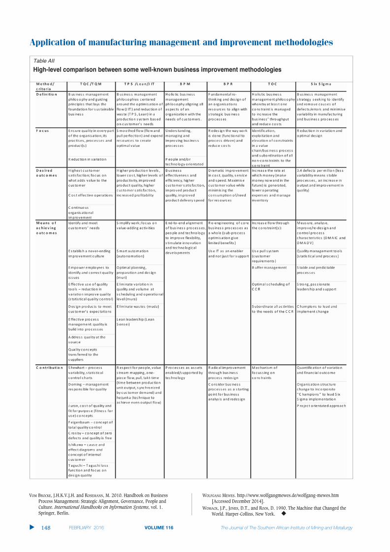
Application of manufacturing management and improvement methodologies
VOM BROCKE, J.H.K.V.J.H. and ROSEMANN, M. 2010. Handbook on BusinessProcess Management: Strategic Alignment, Governance, People andCulture. International Handbooks on Information Systems, vol. 1.Springer, Berlin.
WOLFGANG MEWES. http://www.wolfgangmewes.de/wolfgang-mewes.htm[Accessed December 2014].
WOMACK, J.P., JONES, D.T., and ROOS, D. 1990. The Machine that Changed theWorld. Harper-Collins, New York. �
�
148
Table AII
High-level comparison between some well-known business improvement methodologies
The mining of high gold grades is obviouslyvery beneficial for the economic viability of anoperation, but optimum recovery of theproduct is required to maximize profits(Chapman and Bindoff, 2010, p. 13). Althoughintegrating these two requirements is verydifficult, due to the various activities occurringbetween mining and processing, it isindispensable. The main driver of thisintegration is the impact that different oretypes and characteristics have on head grade.According to Isokangas et al. (2012, p. 871),mining and processing operations involve aseries of well-defined sequential stages thatare complementary in an efficiently operatingmine, with the performance of one operationaffecting that of another. An attempt tooptimize each function separately withoutconsidering the whole extraction process willnot result in the optimum efficiency of theentire mine. Several researchers havedeveloped a proven methodology for revealingthese inefficiencies (Dance et al., 2006, p. 1).
In recent years, JKTech, W.H. BryanResearch Centre (BRC), and the JuliusKruttschnitt Mineral Research Centre (JKMRC)have introduced mine-to-mill integration as aholistic approach to process optimization thatwould maximize the overall profitability(Rogers et al., 2012). Most of these studiesconsidered open pit mining (Ebrahimi, 2013,p. 2) and pit-to-plant operations (Gillot, 2004,p. 1) as subjects and then generalized thesespecific results to underground miningoperations. In most cases, these results werenot applicable to underground gold miningoperations. Despite the interest ininvestigating mine-to-mill integration atindividual gold mines (Bamber, 2008, p. 5;Grundstrom et al., 2001), information on oreloss and dilution is relatively scarce as fewreliable works have been documented that areapplicable to conditions in South African goldmines (Onederra, 2004, p. 1). Moreover, veryfew techniques were previously available tomeasure the size distribution of rockfragments in mining and processing operations(Kanchibotla, Valery, and Morrell, 1999, p.137). It is now possible to simultaneouslyevaluate in-stope fragmentation, monitor oreloss and dilution, and track ore movement indeep-level gold mining.
For the mine to operate efficiently, it isnecessary to compare the actual productrecovered with the desired target. These twoestimations must be as close to each other aspossible; or equated to approximately 100 percent, a situation that is impossible in practice.From a grade control perspective, the multitudeof errors and inaccuracies with regard to theestimated gold content of the reef are hiddenin the mine call factor (MCF) (Chieregati and
Monitoring ore loss and dilution formine-to-mill integration in deep goldmines: a survey-based investigationby L. Xingwana*
The purpose of this study is to understand how ore loss and dilution affectthe mine call factor, with the aim of subsequently improving the quality ofore mined and fed to the mill. It was necessary to know the relationshipbetween ore mined and delivered for processing in order for the mine tooperate efficiently. A review of the literature suggested the mine-to-millintegration approach as a standard intervention to address declining minecall factors. A case study was undertaken at a gold mine in the Free Stateon the influence of the fragment size distribution on ‘free gold’, the effectof ore loss and dilution on the mill efficiency, and time tracking of oremovement from source to the plant. The study revealed thatfragmentation, underground accumulation of ore, and dilution have asignificant influence on the mine call factor and mine output. It wasdifficult to quantify the total ore loss due to the time lag between miningand milling, which is extremely variable, when estimating the mineprocess inventory. However, it was possible to estimate the total dilutionwith some degree of precision by analysing the daily blast and headgrades. It is therefore recommended that mines accept that some gold lossand dilution will always occur during blasting and transport of broken ore,and this loss must be minimized.
Mine call factor, mine-to-mill integration, fragmentation, ore loss, dilution.
* Sibanye Gold, Welkom, South Africa.© The Southern African Institute of Mining and
Metallurgy, 2016. ISSN 2225-6253. This paperwas first presented at the, Mining BusinessOptimization Conference 2015, 11–12 March2015, Mintek, Randburg.
149VOLUME 116 �
http://dx.doi.org/10.17159/2411-9717/2016/v116n2a6

Monitoring ore loss and dilution for mine-to-mill integration in deep gold mines
�
150 VOLUME 116
Pitard, 2009, p. 108; De Jager, 2005, p. 56). From theinvestor perspective, 40% of ore reserves are left behind assupport pillars, and this percentage will increase as the depthof mining increases. Of the 60% remaining and that can bemined, 20% to 30% of the gold-bearing particles are lost inthe chain of operations between the source and processingplant. This issue is further exacerbated by 50% to 100%dilution of the product, which adds to processing costs(Candy, 2014). Focusing on ore dilution to increase headgrade is not a new subject. However, emphasis on generatingmore tonnage to the mill in mining operations has resulted inloss of focus in this area. There is a need to close this gap.
The primary objective of this study was to understandhow ore loss and dilution affect the MCF and to subsequentlyimprove the quality of ore mined and fed to the mill. On thebasis of this objective, the basic research question is:
What is the impact of ore movement on the head grade ina deep-level gold mine?
In subsequent sections. the theoretical framework of thestudy is outlined and the research methodology described.Finally, the paper presents the empirical results of theinvestigation, the main conclusions, and recommendations.
A study by Bamber (2008, p. 5) highlighted two approachesof mine-to-mill integration, namely operational and physicalintegration. Operational integration includes the use of drilland shovel monitoring technologies, optimization of the blastfragmentation and communition processes, and improvedmonitoring in the pit and ore handling system. On the otherhand, physical integration includes fragment sizeclassification, sorting, improving grade control, andimproving mill feed grades. Optimization of the blastfragmentation and improving grade control and feed gradesare the focal points of this study. Based on an analysis of thestudy by Bamber (op. cit.), it was possible to construct amodel of mine-to-mill integration in deep-level gold mines.Figure 1 depicts the impact of the blast movement dynamicson the MCF in a theoretical model.
Figure 1 indicates the three components of mine-to-millintegration, namely fragmentation, ore loss, and dilution,which when addressed on an individual basis would notshow a significant effect on the MCF but when consideredjointly may affect output levels and profit marginsignificantly. The mine therefore needs to optimize blast
fragmentation and to deliver sufficient ore tonnage (volumeand old gold) at the required mill grade (quality and grade)to the metallurgical plant.
Mine-to-mill integration, MCF, fragmentation, ore loss, anddilution may have different connotations for people workingin various mining disciplines, in particular those that are notworking in mineral resource management (MRM) or at themines. These concepts are clarified below.
Mining is a process of delving into the Earth to extractnaturally occurring minerals, either on surface orunderground, and quarrying for construction materials. Forthis study, mining includes the processes of drilling, blasting,and ore movement (handling, loading, and hauling) to themain shaft orepasses.
Milling is the process of crushing, grinding, and treating ofraw material from the mine to extract a saleable product. Italso involves the processes of hoisting and transporting ofbroken ore to the mill via trucks or conveyor belts.
This is an approach to reconcile the blasted material at thestope face with the hoisted raw material at the shaft toprovide accurate information about the quality of ore that isdelivered to the plant. This approach allows the grade controlofficers to reduce the grade variability of the ore sent forprocessing and thus increase the predictability of the goldrecovery. The predictability can be measured based on acomparison of the estimated and actual ore tonnage andgrade. The outcome of this comparison is a factor such as thestope call factor (SCF), shaft call factor, tramming factor,recovery factor, extraction factor, overall recovery factor,plant call factor, and MCF, to name but a few (Chieregati andPitard, 2009, p. 107; Andersen, 1999, p. 4). The emphasis inthis paper is on the MCF.
The mine survey department is responsible for measuringand recording waste and ore broken underground, asindicated in ore flow calculations. All tonnages from differentsources, including surface stockpiles, are added together, andcompared with the actual tonnage received at the plant. Thedifference is known as tonnage discrepancy and is indicatedby the MCF. The MCF is the ratio, expressed as percentage, ofthe specific product accounted for in the recovery, plusresidues, and the corresponding product called for by themine’s measuring and evaluation methods. The objective ofthe MCF is two-fold. Firstly, it is used to investigate whathappened to the ore tonnage and gold content that is notreflected further along the production stream. Secondly, itdetermines how much of the product was lost in theextraction system (Macfarlane, 2011, p. 429; De Jager, 2005,p. 55) or gives an indication of how accurate the estimateturned out to be compared to the quantity of metal recoveredplus residue (Chieregati and Pitard, 2009, p. 107; Minnitt,

Monitoring ore loss and dilution for mine-to-mill integration in deep gold mines
VOLUME 116 151 �
2007, p. 453). These comparisons must be as close aspossible or equate to approximately 100%, a situation that isimpossible in practice, hence a MCF of 85% was consideredreasonable.
The main goal of blasting is to produce manageable rockfragments for ease of cleaning, handling, loading, andcrushing in order to minimize total production costs per tonblasted (Zagreba, 2003, p. 3). Fragmentation may be definedas the size distribution of rock fragments (Cho and Kaneko,2004, p. 1722) and is dependent on the rock properties,specific drill spacing and charge pattern, explosivesproperties, and explosion gas pressure (Cho and Kaneko,2004. p. 1722; La Rosa and Thornton, 2011, pp. 300-302;Thornton, Kanchibotla, and Brunton, 2002). Recent studiestend to support the view that certain explosive types producebetter fragmentation than others, and the MCF can beimproved through better fragmentation (Rajpot, 2009, p. 54).
The movement of ore in the stope is by blasting, facecleaning, gully scraping, and loading from the orepass. Theseprocesses result in some ore not reaching the intendeddestination. Ore loss refers to any unrecoverable economicore left inside a stope (broken, in place as pillars, or notproperly blasted at the boundaries), or to any valuable orenot recovered by the mineral processing system. The tonnageaccumulations consist of current broken ore that is called forby mine measuring methods but was not removed in time tobe incorporated in the current metal accounting system.When this broken ore is finally removed, probably by thevamping section, it is classified as ‘old gold’ and is thencalled for again (Andersen, 1999, p. 15). The failure toremove the ore can create bottlenecks (Rupprecht, 2003, p.53) and causes a low MCF, ultimately complicating the mine-to-mill reconciliation as broken does not reach the surfacetimeously, if at all. Ore losses also arise when valuablematerial is misclassified as waste and sent to the wastedumps (Engmann et al., 2013, p. 27).
The broken material from a stope is a mixture of reef andwaste rock. The proportion of waste to reef depends on manyfactors, including reef width, waste width, faults, intrusions,and mining practices. Dilution may occur as a result of low-grade or waste material mixing with ore during the operationand being sent for processing, thus reducing the ore value(Chieregati and Pitard, 2009, p. 110) or any waste materialwithin a mining block (Yilmaz, 2011, p. 94). Dilution can bequantified as the ratio of the tonnage of waste mined andsent to the mill to the total tonnage of ore plus waste that ismilled (Wang et al., 2011, p. 334). It is always expressed asa percentage:
Waste tons × 100Dilution = Ore plus waste tons
A case study was undertaken at a gold mine in SouthAfrica’s Free State Province of the influence of fragment size
distribution on ‘free gold’, the effect of ore loss and dilutionon the mill efficiency, and time tracking of ore movementfrom source to the plant. The sampling frame was restrictedto all current underground working places, referred to in thisstudy as stope panels. The study was correlational in natureas it was designed to establish the relationship between the actual measurements of the ore hoisted from undergroundand estimates of the ore blasted at the stope faceunderground in order to improve the MCF. Specifically, theaim was to predict quantitatively the effect of ore handlingand transport on the ore grade sent to the plant anddetermine the statistical significance of the estimatedrelationships. This would be possible with the application ofthe mine-to-mill approach considering in-stopefragmentation, dilution, ore loss, and tracking in the form offour exercises.
The first exercise examined the size distribution of rockfragments to minimize and control loading, hauling, andcrushing costs, using digital photography and directobservation. Twenty images of broken ore in stopes 4 and 6were used to measure the size distribution of blastedfragments. According to Siddiqui, Ali Shah, and Behan(2009, p. 83), image acquisition is crucial in the analysis offragment size distribution. The images were taken randomlyand systematically, at an angle that ensured the surfaces offragments were photographed in full, while balls of 20 mm indiameter and tennis balls were used to provide the scale ofthe images at the stope face, gully, boxhole vicinity, andcrosscut. These images were then downloaded into the SPLITDesktop program for analysis. According to Siddiqui, et al.(2009, p. 83), there are several software packages, such asSPLIT, GoldSize, FragScan, PowerSieve, etc. that arecommercially available to quantify size distribution. Therationale behind choosing SPLIT Desktop for size distributionwas that the accuracy of these systems is presumed to bebetween 2% and 20%. To check the reliability of visualobservations of the muck pile underground, online digitalcameras were mounted at a strategic point on surface. Thesecameras automatically captured images of ore on a movingconveyor belt, analysed the size distribution of the rocks withthe SPLIT image analysis system, and reported the rock sizestatistics and passing percentage.
The second exercise was the gap analysis that would helpthe business understand and quantify the grade gap thatexists between the estimate of mine production and actualgrade entering the plant. The data was collected throughobservation and grab sampling methods. Grab samples werecollected at the top, middle, and bottom of the stope face andat the cross-section of various points (strike and dip gullies)and the mean value of these points was used for the analysis.The representativeness of these samples was considered fairinsofar that they represented high-, medium-, and low-gradepanels and were sufficient to indicate the grade gap along theore stream. For this study, a SCF score of 60% or more wasconsidered to be practically significant and to confirmconvergent validity. Grab sampling was used as a method ofreconciling the daily blasted grade to the predicted daily headgrade (Dominy, 2010, p. 277) and not for metal accountingpurposes (Spangenberg, 2012, p. 73). Numbered samplesweighing about 500 g each were collected from muck piles ofbroken ore at the stope face, gully cross-sections, boxhole,

Monitoring ore loss and dilution for mine-to-mill integration in deep gold mines
and crosscut. The samples were securely packed, transportedto the assay laboratory, and assayed to determine gold andsilver values. This method of grab sampling was used withextreme caution to avoid over-sampling of fines, pick-up, andpreferential selection of high-grade fragments. For instance, alarge sample was drawn, reduced to the required size of 500 g by quartering, and then sent to the assay laboratory. Inthis way, more representative samples were obtained.
The third exercise was the process system analysis usinga material census checklist as the measuring instrument. Therationale behind this step was to pinpoint flaws in the gradecontrol methods and examine whether the grade controlsystem was properly established, operated at maximumefficiency, and all MCF requirements were addressed. Thisexercise covered observations from a series of undergroundvisits to several stoping panels. A considerable time wasspent in the working place, taking field notes of what wasoccurring. The checklists were developed to assess four areasof concern, namely the stope face, advance strike gully,central dip gully, and orepass for possible accumulation ofore. Although material census checklists were usedextensively as the measuring instruments, the study relied onthe experience of the researcher to identify these areas ofconcern from the ore flow diagram.
The fourth exercise was concerned with the tracking ofore movement from the stope face to the stope orepass. Radiofrequency identification (RFID) tags were used as trackingdevices (Isokangas et al., 2012 p. 874) to:
� Identify the source of ore with a high fines content;� Indicate how long it took for the ore to be hauled to the
surface� Record any cross-tramming events over time with great
accuracy.
These numbered RFID tags have a chip with an antennaencased in a hard protective plastic shell to withstand theblasting and handling process en route to the mill plant. Thetag number, the stope location where the tag was placed, thename of the surveyor, time and date, as well as shaft wereentered into the database. The characteristics of the ore at theparticular source were recorded in the field notebookunderground. The RFID tags were dropped on the brokenrock at the stope face and in the advance strike gully, centre
gully, and boxhole. These tags surfaced from undergroundwith broken ore on the conveyor belt, where a tag detectorrecorded and passed the information to the database. Amanagement report was extracted from the database toassess the time taken for the waste and reef to reach surface.Tagged ore sent to stockpiles can be detected at a later stagewhen eventually processed and then reconciled back to itssource.
Since the main concerns in reliability and validitymeasurements were stability over time or variability ofconditions, a common way to estimate reliability andconvergence validity was with a measure of association andthe correlation coefficient.
The data obtained from stopes 4 and 6 was transferred to anExcel spreadsheet and analysed using Microsoft Excel 2013.Data was analysed by means of descriptive statistics,correlations, and regression analysis.
As a problem-solving tool, the mine-to-mill integrationapproach followed a particular business ore flow sheet thatshows the various stages that the ore passes through beforethe final product is extracted. The ore flow sheet guided thesequence of analyses that the study used to indicate where tostart and end measuring. The investigation begins withunderstanding of in-stope fragmentation for mine-to mill-integration model standardization. This is followed by valuestream mapping and monitoring of ore loss and dilution.Finally, the investigation closes with time tracking of oremovement from source to the mill plant.
An understanding of fragmentation was obtained first byvisual observations of muck piles immediately following theblasting of rock in situ, and the SPLIT offline applicationsused to predict the size range of the actual blasted rocks (seeFigure 2). Since 20 mm rubber balls, tennis balls, andgrizzlies were used as scaling tools, an image analysisstrategy was developed that estimated the size distribution of
�
152 VOLUME 116

the broken ore across the percentage <20 mm (fines) andpercentage >20 mm (coarse) fragments. This strategy issummarized in Figure 2; the actual details of this process arebeyond the scope of this paper.
Figure 2 indicates that the size distribution of fines waspositively correlated (from 53% to 68% split of ore material)with the movement of broken ore. This means that theamount of fines increases as the broken ore moves awayfrom the source. On the other hand, the size distribution ofcoarse particles is negatively correlated (from 47% to 32%split of ore material) with the movement of broken ore. Thismeans that the amount of coarse particles decreases as thebroken ore moves away from the stope face to the BH. Amean fragment size of less than 20 mm at sieve passing rateof 74% was observed in the crosscut. Therefore, the finesdistribution of data of this bar chart is negatively skewed (tothe left), while the coarse distribution is positively skewed (tothe right). However, it must be noted that the mean size ofthe coarse distribution might be smaller than that estimatedfrom visual inspection, since smaller fragments dominatedthe view after vibration and settling. Therefore, for this stopepanel, 68% of the gold-bearing particles were liberated fromthe host rock (quartz, silicates, and pyrite) while 32% of thecoarse particles were associated with or still attached to thehost rock. Hence there was a need to reduce the amount offines in the blasted material and optimize fragmentation.
An investigation of fines distribution at the stope faceindicated that the friable and carbonaceous portion of thereef, which contains the highest portion of gold, was the mostshattered by blasting, broken out, and crushed into fineseasily. In contrast, gangue (waste material) was mostlybigger than tennis ball size, hence the ore and waste werebroken unequally. The substantial rock breakage was furtherexacerbated by the increase in panel length, gully length,scraper routes, and crossovers that caused the decrease incleaning rate. The more the cleaning rate decreases, the morethe coarse particles are crushed further into fines. It must benoted that gold particles are minute, associated with very fineparticles, and can be as fine as 0.001 mm. These finesbecome airborne and are dispersed by gaseous emissions asdust from the collection zone when the rock is blastedconventionally. These fines could also be easily water-washed into crevices and cracks in the footwall or away todifferent parts of the mine during sweeping or drilling, thusincreasing gold loss. The gold lost underground in this
manner is commonly referred to as ‘free gold’. Free gold hasbeen a persistent problem in the mine for some time, asdemonstrated by significant higher gold recoveries from thefines in the back area and mud in the crosscuts. Hence therewas a need to understand the run-of-mine fragmentation.
The visual observations of the muck pile underground werecompared with the actual fragmentation results from imageanalysis captured from the online digital camera throughSPLIT online applications (see Figure 3).
The results in Figure 3 show a mean fragment size of16.00 mm at 50% passing. In addition, the shape distributionof these fragments is consistent and negatively skewed,whereby mean% < median% < mode, indicating a finer sizedistribution. The greatest increase in fines content occursbetween 3 mm and 10 mm as well as between 50 mm and100 mm, as shown by the steepness of the curve betweenthese class boundaries. Hence, approximately 92.17% of thefragments will not require crushing as they will passsmoothly through the primary crusher to the secondarycrusher screen. This means there a greater percentage of finerfragments was fed to the mills on 4 of July. It is clear fromFigures 2 and 3 that the estimates of size distribution offragments in both cases are very close to each other.
The choice of using Anfex explosives in developmentends and Powergel (cartridge) explosives in stope panels wasmainly based on rock breakage requirements. Subsequently,drilling patterns and overcharging remain the cause of theincreased fragmentation that leads to losses of gold in thefine fractions produced. The production of excessive of finematerials and dust is not desirable in gold mines in that it:
� Poses a health hazard to the workers underground (acause of silicosis and tuberculosis)
� Is not easy to collect in subsequent scraping, loading,and hauling operations, leading to losses of gold.
The blasted broken ore in the stopes is a mixture of wasterock and gold-bearing rock (reef). No matter how careful thepersonnel are to mine only reef, there will always be wasterock diluting the grade of ore going to the mill for processing.A gap analysis report of eight stope panels (Table I) wasprepared to assist mine management understand why the oretonnage and gold content were not being reflected furtheralong the production stream.
Monitoring ore loss and dilution for mine-to-mill integration in deep gold mines
VOLUME 116 153 �

Monitoring ore loss and dilution for mine-to-mill integration in deep gold mines
Table I shows that all SCF score values for the eight stopepanels are above 60% and that the values of chip and grabsamples are practically significant, related to each other, andconfirm the convergence validity of the techniques. However,since grab samples were collected from the fines, grabsampling tended to overstate the grade of the diluted wasteblock by 14.29% to 160.5% and understate the grade of thehigh-grade block by 8.54% to 81.34%. Even though theassay values of these stope panels were variable, most of thegold particles were located in the fines and this is a cause ofconcern for the mine-to-mill reconciliation and metalaccounting system. The grade variability of the mine-to-millintegration model was explained by dilution, which can be upto 100% where off-reef is mined.
On investigation, it was found that the gold mineralization isassociated with weak host rock and geological features suchas faults, sills, and dykes. Deposits within weak host rockswith indistinct contacts are usually associated with caving ofsidewalls and the hangingwall, resulting in high dilution. Itwas also observed that where an ideal stoping width wasmaintained, drilled holes were drilled into the narrow reef.
During blasting the gold-bearing material was scattered farand wide in the stope panel, leaving behind large quantity ofwaste rock. Evidence of this was in the form of the high goldcontent of the fines that covered mat packs and contaminatedthe swept area. In addition to the large quantity of waste rockbroken from the stope face, it is important to consider alsothe waste from footwall scraping during cleaning, barring ofbrows, and falls of ground, faults, intrusions, and footwalllifting in gullies. These waste materials contaminate the orein the downstream process. However, an overall analysis ofgold concentration at the face, and in the gullies andorepasses (hoppers to the station) (Table II) indicated thatthe assay values had a significant positive correlation, with acoefficient of 0.9291 (Table III).
Although it is impossible or impractical to eliminate dilutioncompletely, it can be measured (Figure 4) and controlled(Figure 5) with some degree of precision. What is required isfor the orebody to be properly delineated and the extractedvolumes to be effectively measured. It is a common practice tomake general assumptions of 5% dilution for massivedeposits and 10% for tabular deposits, instead of measuring
�
154 VOLUME 116
Table I
Grade gap analysis report
Panel Stope ASG CDG Av. (grab) Av. (chip) Boxholes X-CUT SCF Grade gap
1 Stope 4 7.400 10.119 9.470 9.411 8.033 11.478 8.673 117.30% +14.29%15.0m (M/P) 10.655 Water Overstate
2 Stope 5 4.018 4.566 4.303 5.233 3.701 6.561 82.22% -8.54%11.5m (M/P) 4.755 Understate
3 Stope 6 5.434 3.725 3.552 4.763 6.933 3.107 3.194 68.70% -81.34%14.0m (S/A) 6.342 Understate
4 Stope 7 13.207 10.538 7.163 12.410 16.167 9.426 7.245 76.76% -51.87%14.5m (S/A) 18.604 Water Understate
5 Stope 8 9.191 5.697 7.289 7.630 9.100 6.902 7.781 83.84% -14.49%14.0m (M/P) 8.343 Water Same CG Understate
6 Stope 9 3.695 3.475 3.175 3.184 5.000 5.058 7.059 63.68% +11.60%15.0m (S/A) 2.392 Overstate
7 Stope 10 3.944 2.473 1.953 2.239 0.700 1.556 2.400 319.86% +122.3%13.0m (M/P) 0.584 Overstate
8 Stope 11 4.467 2.400 4.800 3.715 0.600 1.563 2.791 619.17% +160.5%18.0m (S/A) 3.191 Overstate Overstate
M/P = Mat packs S/A = Swept area
Table II
Tonnage inventory of underground accumulation of broken ore
Stope face (RD = 1.62) Advance strike gully (W = 2.0m) Central dip gully (W = 2.0m) Boxhole (W = 1.4m)
L B H Tons L H Tons L H Tons L H Tons
Stope 4 41 24 0.6 956 126 1.0 408 35 0.9 102 33 2.0 150
Stope 5 28 10 0.3 136 98 1.0 318 5 1.1 18 27 2.0 122
Stope 6 24 10 0.5 194 47 0.3 46 30 0.7 68 21 2.0 95
Stope 7 25 10 0.3 122 35 0.4 45 5 0.8 10 17 2.0 77
Total 1408 817 198 227
Total = 2650 t

it (Ebrahimi, 2013, p. 1). This assumption differs from mineto mine. The comparison of daily head grade and dailyblasted grade is depicted in Figure 4.
From a comparison of the total mine daily blasted gradeand the plant head grade (Figure 4), it is obvious that gradevariation does exist, although the overall pattern is quitestable with few outliers such as 10.25 g/t (13 June), 10.45g/t (21 June), and 9.36 g/t (3 July). A monthly gradevariation of approximately 52.59% due to dilution is shown,and can be used to estimate the dilution rate for theforthcoming months, provided that corrective measures areimplemented. This means that the daily blasted grade wouldalways be greater than the daily head grade; therefore theMCF would always be less than 100%. An investigationregarding the discrepancy between the estimation of dailyhead grade and daily blasted grade is beyond the scope ofthis study. The answer to this might lie in the fact that theestimates of shaft head grade include the grades ofdevelopment ore (waste and reef), sweepings from old areas,and other sources, not all of which were sampled (Bartlett,Korff, and Minnitt, 2014, p. 109). The grade of broken orehoisted from underground (daily head grade) is notequivalent to the grade measured on the faces (daily blastedgrade)
Figure 5 demonstrates how dilution can be controlled fora properly delineated orebody.
Figure 5 indicates that in December, an average reefchannel width of 17 cm was mined out with 130 cm ofexternal waste, resulting into a dilution of 88.4%. The annualdilution of this unit ranges from 68.6% to 89.6%, the peakbeing in September. Over a twelve-month period, the reef wassteadily becoming thinner. Subsequently, as miningprogresses, more waste would be included in the muck pilesand the mill feed grade would decrease. A grade of 24.6%gold was reported in January, decreasing to 13.0% inDecember. In this way dilution can be measured and can becontrolled by reducing external waste. The financial impact ofdilution on the mining operation is due to the extra costsinvolved in mining and processing of the waste (130 cm) thatis treated as ore.
An ore with a dilution rate of 88.4% should not be sent tothe mill for processing, but action must be taken to separatewaste from the ore either underground or on surface. If thisis not possible, then this material must be treated as wasteand dumped. For instance, if the processing cost was R200per ton, a dilution rate of 88% would mean that R176 isspent on processing waste as ore in the mill. It is clear thatthe mill processing costs would increase directly by an
Monitoring ore loss and dilution for mine-to-mill integration in deep gold mines
VOLUME 116 155 �

Monitoring ore loss and dilution for mine-to-mill integration in deep gold mines
amount equal to the dilution factor. Reduction of externalwaste would result in less tonnage at a higher grade beingsent to the plant. This dilution of ore with waste would meanlow-grade ore will be processed instead of high grade ore.This would impact negatively on the MCF.
As discussed previously, gold losses occur when gold-bearingmaterial is misclassified as waste and sent to the wastedump, reef is left behind in the footwall and hangingwall,excessive waste is mined, blocks of reef are left behind aspermanent support pillars, and ore locked up underground isnot removed in time to form part of the current metalaccounting system. The latter factor is the focus of this study.The real gold loss must be found underground, if the lossoccurs during mining operations, but if it cannot be foundunderground it can only be ascribed as apparent gold loss.Table II is a hypothetical, but realistic, example to illustratehow much of the gold-bearing material was lost in theextraction process.
Table II indicates that there was accumulation of brokenore at the faces in stopes 4 and 5, gullies, and orepass duringthe movement of ore. The movement of ore in the stope is theresult of blasting, face cleaning, gully scraping, and loadingfrom the orepass. These are the potential areas of tonnageaccumulation. The tonnage accumulations consist of currentbroken ore that is called for but was not removed in time toform part of the current metal accounting system. Theinability to locate the exact points of accumulation of oreunderground and quantify the volume and value of gold-bearing material remaining underground over time has led toa declining MCF.
On investigation, it was found that the accumulation of oreunderground was due to the long face length and scrapingdistance in the gully. As the gully length, scraper routes, andcrossovers increase, the more the cleaning rate decreases andcoarse particles are crushed further into fines. Work ingeneral, in particular scraper cleaning, becomes difficult,leading to the accumulation of ore in the back area, sidings(north and south) and gullies. This indicates that sweeping ofback area was not done on daily basis as part of the mining
cycle. If panels are not timeously swept, falls of ground mayoccur and cover up vast areas of backlog sweepings that willnever be removed due to safety issues. Excessiveaccumulation of material in the gully reduces the gully depthif not pulled to the footwall regularly. A shallow gully hasinsufficient storage capacity when an orepass is filled up dueto tramming delays, resulting into spillage along theshoulders and adjacent swept panel, amounting to gold loss.This means that these gullies would not be scraper-cleaned tothe footwall regularly. Two of the reasons that were noted fornot scraping the gully to the footwall regularly were offlinedevelopment of the gully and the use of 37 kW winch withone scoop to clean the scraping distance of more than 60 m.The offline gullies observed created major cleaningbottlenecks associated with damaged gully shoulders, largegully span, accumulation of broken ore, water in the gully,and spillage along the shoulders of the gully.
Figure 6 indicates how accurate the estimate turned out to becompared to the quantity of metal recovered plus residue.
Figure 6 indicates that the estimated hoisted gold andgold recovered at the plant show parallel trends over time; theincrements of the two variables are the same and there is anore loss or overestimation of about 17% (in kilograms)between the underground source to the surface plant. Thismeans that more tonnage with low grade was sent to the millfor processing, resulting into low overall recovery. A MCF of83% seems justified to estimate the amount of gold to berecovered in forthcoming months, provided that all othervariables stay the same.
In an attempt to ascertain the impact of ore movement on thehead grade at the mine, correlation and regression analysiswere applied.
The current study was correlational in nature as it wasdesigned to assist understanding of how gold was lostbetween the source (stope face) and the shaft main tips. Thecorrelation coefficient is one of the techniques used toestimate reliability of this study by measuring the correlation
�
156 VOLUME 116

between the distance from the source to the shaft and thegold content. The discussion above showed that the sizedistribution of fines was positively correlated and the coarsenegatively correlated, but this is only a qualitative indication.The correlation coefficient provides a quantitative measure ofthe relationship. For example, the correlation coefficients forstopes 4 and 6 are presented in Table III and Figures 7 and 8.
There is a positive correlation coefficient of 0.9130between distance and grade as the broken ore moves fromstope to the shaft main orepass, and a negative correlationcoefficient of -0.97079 in the case of stope 6. A highcorrelation coefficient indicates a convergent validity. Apositive relationship shows that as the distance from thestope face to the orepass increases, so does the fines content(gold content) of the broken ore. Since both correlationcoefficients are close to unity, there is a strong correlationbetween the gold content and distance between the sourceand main shaft orepass.
Regression analysis was performed to determine the extent towhich the distance to the main shaft orepass would explainthe variance in grams per ton (value) of the ore broken fromthe stope face. The discussion deals with the application ofregression to firstly estimate or predict the quantitative effectof the distance upon the values, and secondly to determinethe statistical significance of the estimated relationships. The summary of the Excel regression output is presented in Table IV (for the case where gold is evenly distributed overthe width of the reef) and Table V (gold is concentrated nearthe footwall contact of the reef).
In Table V, the R2 value of 0.833 indicates that most ofthe data has some linear relationship, with some degree ofscatter; a very good fit as R2 is close to unity. This means83% of the variation in the grade is explained by the lengthof the gully. However, the relationship between these twovariables is statistically insignificant at a significance level = 0.05 as p > 0.05, with P-value = 0.0870 despite thecorrelation coefficient of 0.913. This means that the distanceof movement of ore from a thick reef (where gold is evenlydistributed over the width) does not have an adverse effecton the grade gap. In other words, for each unit increase inlength at 7.385 Y-intercept, the grade increases by 0.019units.
In Table V, R2 the value of 0.942 indicates that most ofthe data has some linear relationship, while some isscattered, a very good fit as R2 is closer to unity. This meansthat 94% of the grade variation is explained by the length ofthe gully. The table also show that the relationship between
the length and grade is statistically significant (p < 0.05, withquantitative effect of 0.0292) despite an inverse relationshipof -0.97079. This means that the distance of movement ofore from a thin reef (where gold is concentrated near thefootwall contact) does have an adverse effect on the gradegap. In other words, for each unit increase in length at 4.708Y-intercept, the grade decreases by 0.016 units. It cantherefore be deduced that the grade gap between the sourceand the plant is very variable due to the uncertainty of manygrade-controlling parameters, in particular the dynamics ofore movement.
Having tested the relationship between the transportdistance and grade, it is now possible to determine the timelag between the measuring and milling month and track thesource of material being fed into the crushing and grindingcircuits.
Monitoring ore loss and dilution for mine-to-mill integration in deep gold mines
VOLUME 116 157 �
Table III
Determining correlation coefficient of Stope 4 and 6
Stope 4 Stope 6
Distance from face (cumulative) Grams per ton Distance from face (cumulative) Grams per ton
Stope face 0 7.4 0 4.8Adv. strike gully 126 10.1 47 3,7Central dip gully 161 9.5 77 3,6Box hole 181 11.5 98 3;1

Monitoring ore loss and dilution for mine-to-mill integration in deep gold mines
The real gold loss must be traceable if lost during miningoperations, but if it cannot be located underground it can onlybe ascribed as apparent gold loss. It is of vital importance thatmovement of ore from the source to the mill is understood toreduce ore loss and dilution in order to improve the MCF.Table VI depicts the time lag between undergroundproduction and milling.
Table VI indicates the time the RFID tags were planted inthe muck piles at the source and the detection time at theconveyor belt on surface. The fluctuations in the monthlymined value and the time lag of approximately 20 daysbetween production and milling also result in variations inthe MCF. The time delays may therefore be extremelyvariable, making it difficult to estimate the mine processinventory and develop a metal accounting system with a fairdegree of confidence. Only one reef tag (A5756) was read at22h56 as going to the waste dump. This means gold-bearingmaterial is still classified as waste and sent to the wastedump, a potential loss of gold. The highlighted tags were
those that correspond to top ten high-grade panels of theirrespective shafts and their low recovery rates indicate thathigh-grade ore does not reach surface timeously, if at all. Theslow arrival of high-grade ore causes a low MCF andcomplicates mine-to-mill reconciliation. The financial impactof ore loss on the mining operation equals the revenue that isforfeited when ore is not delivered from the mine to the plant.With this information, corrective measures can be takenquickly. Ore tracking reports are sent on a weekly basis to themanager, listing the tags that have not yet passed the reader.If the tracking system is effective, ore loss and dilution can beestimated by correlating the time the tag was dropped at thestope face and the time it was detected on the conveyor belt.For tags A5711 and A5712 movements of 181 m and timelags of 15 days were recorded, and these have significantimplications for dilution and ore loss. The inability to locatethe exact points of ore accumulation underground and toquantify the volume and value of gold-bearing materialremaining underground over time has led to a declining MCF.
�
158 VOLUME 116
Table IV
Regression analysis: Influence of distance on grade value of Stope 4
Regression statistics
Multiple R 0,912961608R Square 0,833498897Adjusted R Square 0,750248346Standard Error 0,851413047Observations 4
ANOVA
df SS MS F Significance F
Regression 1 7,257691647 7,257692 10,01193245 0,087038392Residual 2 1,449808353 0,724904Total 3 8,7075
Coefficients Standard Error t Stat P-value Lower 95% Upper 95% Lower 95,0 Upper 95,0
Intercept -302,0453632 133,9817346 -2,25438 0,152886 -878,522 274,4315 -878,522 274,4315Value 43,53718059 13,7594586 3,164164 0,087038 -15,665 102,7394 -15,665 102,7394
Table V
Regression analysis: Influence of distance on grade value of Stope 6
Regression statistics
Multiple R 0,970786114R Square 0,94242568Adjusted R Square 0,91363852Standard Error 0,210552194Observations 4
ANOVA
df SS MS F Significance F
Regression 1 1,451336 1,451336 32,73771 0,029213886Residual 2 0,088664 0.044332Total 3 1.54
Coefficients Standard Error t Stat P-value Lower 95% Upper 95% Lower 95,0 Upper 95,0
Intercept 274,3701299 38,75931612 7,078818 0,019378 107,6022525 441,138 107,6023 441,138Value -57,5974026 10,06650595 -5,72169 0,029214 -100,9100819 -14,2847 -100,91 -14,2847

This study was aimed at increasing mine output and profitmargin by controlling fragment size distribution, managinggrade variability, and ensuring that broken ore reaches themill plant timeously. Movement of rock, ore loss, and dilutionare the consequence of blasting the rock in situ. Hence,efficiency ore management mine necessitates the need tomeasure accurately, firstly the fragment size distribution,then ore loss and dilution, and thereafter track ore movementafter blasting from the stope face to the concentration plant.The findings of the study have shown that it is difficult toquantify the total ore loss due to the time lag betweenbreaking of the rock and processing of the ore to the finalproduct when estimating the mine process inventory. Theinability to minimize ore loss can thus impact negatively onmine output through the loss of revenue. However, it ispossible to estimate the total dilution with some degree ofprecision by analysing the daily blast grade and daily headgrade. Ore dilution can also impact negatively on the mineprofit margin as a result of the extra costs involved in miningand processing of the waste that is treated as ore. The feed tothe concentrator should preferably contain a sufficientamount of high-grade gold ore and be as homogeneous aspossible for stable plant operation. However, ore below thepay limit adds variation to the mill grade as increased millthroughput will be required to make up for the loss of gold,and that impacts on the recovery in the plant. It is againstthese perspectives and findings of this study that the MCFshould be seen as a method that identify the real problemsunderground and when these are addressed, the profitabilityof the mine will increase.
A satisfactory mine output and margins can be achievedby the correct application of the mine-to-mill approachdiscussed above. It is therefore recommended that the mineaccept that ore losses and dilution will always occur duringblasting and moving of broken ore, and this loss must bekept at a minimum. It is worth mentioning that a MCFinvestigation is likely to be successful when initiated andsupported by management.
� The focus in this research was on real gold lossbetween the source and the stope orepass. It wouldhave been useful and interesting to analyse therelationship between the apparent gold loss and themine call factor
� The empirical study was carried out for academicpurposes and therefore the time allocated was limited,hence a cross-sectional survey was performed. The trueresults could have been obtained through alongitudinal study and testing of reversal causal effects
� Three short case studies were undertaken tounderstand the impact of ore loss and dilution on theMCF. This situation varies widely from mine to mine,depending upon the problems posed and managerialpolicy. The ability to extend the results of the study tothe wider South African mining industry is thereforelimited
� RFID tags were place at the working place in the reefhorizon only. Information regarding the classificationof waste as reef could have been obtained to minimizedilution of broken ore sent to the mill
� Due to the limited availability of resources and timeallocated for this project, it was not possible to visit allstope working places.
The following extract seems appropriate to conclude thispaper with:
‘… for a higher grade deposit, the cost of ore loss andmisclassification has a greater impact than the cost ofdilution, hence it may be preferable to accept moredilution to minimise the cost of ore loss andmisclassification’ and ‘… for a lower grade deposit, thecost of dilution has a greater impact than the cost of oreloss…, hence it may be preferable to accept more ore lossand misclassification to minimise the cost of dilution…’(Singh and Sinha, 2013, p. 263).
My thanks to Chris Opperman, Ndubuzo Shange, andLazarus Phutheho for their contributions to this study.
Monitoring ore loss and dilution for mine-to-mill integration in deep gold mines
VOLUME 116 159 �
Table VI
Management ore tracking report
Reader Read date Read time Tag ID Surveyor Working place Panel no. Issue date Issue time Time, days
2R Belt 14-Jun 04H08 A5638 John Stope 01 BH 13-Jun 9H00 1
2R Belt 15-Jun 17H24 A5637 John Stope 01 FACE 13-Jun 9H10 2
2R Belt 14-Jun 14H25 A5641 John Stope 02 BH 11-Jun 9H00 3
2R Belt 26-Jun 09H14 A5631 John Stope 02 FACE 11-Jun 10H00 15
2R Belt 12-Jul 06H44 A5632 John Stope 03 FACE 12-Jun 9H00 30
2R Belt 21-Jun 01H30 A5633 John Stope 03 ASG 12-Jun 9H00 9
3R Belt 4-Jul 16H30 A5711 John Stope 04 FACE 19-Jun 9H00 15
3R Belt 4-Jul 16H12 A5712 John Stope 05 FACE 19-Jun 9H10 15
3R Belt 5-Jul 03H15 A5715 John Stope 06 FACE 19-Jun 9H30 16
4R Belt 21 Jun 15H51 A5751 John Stope 07 SSG 21-Jun 9H35 0
4R Belt 2-Jul 16H46 A5752 John Stope 07 FACE 21-Jun 9H00 11
5R Belt 30-Jun 22H56 A5756 John Stope 08 BH 21-Jun 9H50 9
4R Belt 7-Jul 19H29 A5757 John Stope 08 FACE 21-Jun 9H45 17
4R Belt 28-Jun 01H45 A5758 John Stope 09 FACE 21-Jun 9H40 7
4# Reef 30-Jun 18H14 A5759 John Stope 09 ASG 21-Jun 9H45 9

Monitoring ore loss and dilution for mine-to-mill integration in deep gold mines
ANDERSEN, D.C. 1999. Criteria influencing the mine call factor of a gold mine.
Selected topics in mining engineering. Faculty of Mining Engineering,
University of the Witwatersrand, Johannesburg.
BAMBER, A.S. 2008. Integrated mining, pre-concentration and waste disposal
systems for the increased sustainability of hard rock metal mining.
Doctoral thesis, University of British Columbia, Vancouver.
BARTLETT, H.E., KORFF, L., and MINNITT, R.C.A. 2014. The allocation of gold
production from multiple shafts feeding a common treatment plant using
run-of-mine sampling of ore deliveries. Journal of the Southern African
Institute of Mining and Metallurgy, vol. 114. pp. 109–120.
CANDY, G. 2014. New tech to help gold miners tackle tough veins. Mineweb.
CHAPMAN, R. and BINDOFF, M. 2010. The placer gold mining game. School of
Earth and Environment, University of Leeds:
CHIEREGATI, A.C. and PITARD, F.F. 2009. The challenge of sampling gold.
Proceedings of the Fourth World Conference on Sampling and Blending.
Southern African Institute of Mining and Metallurgy, Johannesburg.
CHO, S.H. and KANEKO, K. 2004. Rock fragmentation control in blasting. Mining
and Materials Processing Institute of Japan, vol, 45, no.5. pp. 1722–1730.
DANCE, A., VALERY, W., JANKOVIC, A., LA ROSA, D., and ESEN, S. 2006. Higher
productivity through cooperative effort: A method of revealing and
correcting hidden operating inefficiencies. Proceedings of SAG 2006,
Vancouver, 23-27 September 2006. CIM, Montreal. pp IV–375.
De Jager, C.P. 2005. Risk management in mining and minerals economics as
well as minerals resources management. Master’s dissertation. University
of the Witwatersrand, Johannesburg.
DOMINY, S.C. 2010. Grab sampling for underground gold mine grade control.
Journal of the Southern African Institute of Mining and Metallurgy,
vol. 110. pp. 277-287.
EBRAHIMI, A. 2013. The importance of dilution factor for open pit mining
practices. [A modified version of: An attempt to standardize the
estimation of dilution factor for open pit mining projects]. Proceedings of
the World Mining Congress, Montreal.
ENGMANN, E., AKO, S., BISIAUX, B., ROGERS, W., and KANCHIBOTLA, S. 2013.
Measurement and modelling of blast movement to reduce ore losses and
dilution at Ahafo Gold Mine in Ghana. Ghana Mining Journal, vol. 14.
pp. 27–36.
ISOKANGAS, E., SONMEZ, B., WORTLEY, M., and VALERY, W. 2012. Using Smarttag
to track ore in process integration and optimization projects: Some case
studies in a variety of applications. Journal of the Southern African
Institute of Mining and Metallurgy, vol. 112. pp. 871–892.
GILLOT, P.L. 2004. Pit-to-plant optimisation at Morila Gold Mine. Morila Gold
Mine, Bamako, Ghana.
GRUNDSTROM, C., KANCHIBOTLA, S.S., JANKOVICH, A., and THORNTON, D. 2001. Blast
fragmentation for maximising the SAG mill throughput at Porgera Gold
Mine. Julius Kruttschnitt Mineral Research Centre, Brisbane.
KANCHIBOTLA, S.S., VALERY, W., and MORREL, S. 1999. Modelling fines in blast
fragmentation and its impact on crushing and grinding. Proceedings of
Explo’99. Australasian Institute of Mining and Metallurgy, Melbourne.
pp. 137–144.
LA ROSA, D. AND THORNTON, D. 2011. Blast movement modelling and
measurement. Proceedings of the 35th APCOM Symposium, Wollongong,
New South Wales, 24–30 September.
MACFARLANE, A. 2011. Reconciliation along the base metal value chain.
Proceedings of the 6th Southern African Base Metals Conference. Southern
African Institute of Mining and Metallurgy, Johannesburg. pp. 345–356.
MINNITT, R.C.A. 2007. Sampling: the impact on costs and decision making.
Journal of the Southern African Institute of Mining and Metallurgy,
vol. 107. pp. 451–462.
ONEDERRA, I. 2004. Breakage and fragmentation modelling for underground
production blasting applications. Julius Kruttschnitt Mineral Research
Centre, University of Queensland, Australia.
RAJPOT, M.A. 2009. The effect of fragmentation specification on blasting cost.
Master’s thesis, Queen's University, Kingston, Ontario, Canada.
ROGERS, W., KANCHIBOTLA, S.S., TORDOIR, A., AKO, S., ENGMANN, E., and BISIAUX, B.
2012. Solutions to reduce blast-induced ore loss and dilution at Ahafo
Gold Mine in Ghana. Proceedings of the 2012 SME Annual Meeting and
Exhibit 2012, Seattle, Washington. Preprints, pp. 19–22.
RUPPRECHT, S.M. 2003. Best practice for personnel, material and rock
transportation in ultra-deep level gold mines. Doctoral thesis, University
of Natal, Durban.
SIDDIQUI, F.I., ALI SHAH, S.M., and BEHAN, M.Y. 2009. Measurement of size
distribution of blasted rock using digital image processing. JKU
Engineering Science, vol. 20. no.2. pp. 81–93
Singh, P.K. and Sinha, A. 2013. Rock Fragmentation by Blasting. Taylor &
Francis, London.
SPANGENBERG, I.C. 2012. The status of sampling practice in the gold mining
industry in Africa: Working towards an international standard for gold
mining sample practices. Master’s dissertaton, University of the
Witwatersrand, Johannesburg.
THORNTON, D.M., KANCHIBOTLA, S., and BRUNTON, I.D. 2002. Modelling the impact
of rock mass and blast design variation on blast fragmentation. Fragblast,
vol. 62. pp.169–183.
WANG, W., HUANG, S., WU, X., and MA, O. 2011. Calculation and management
for mining loss and dilution under 3D visualization technical condition.
Journal of Software Engineering and Applications, vol. 4. pp. 329–334.
YILMAZ, E. 2011. Advances in reducing large volumes of environmentally
harmful mine waste rocks and tailings. Department of Applied Sciences,
University of Québec at Abitibi-Temiscamingue (UQAT).
ZAGREBA, S.V. 2003. FRAGM: A blasting fragmentation model of rocks,
Master’s thesis, Department of Mining Engineering. West Virginia
University. �
�
160 VOLUME 116

The geoelectrical resistivity method has beenwidely used since the early 20th century, andplays an important role in several fields suchas groundwater and subsurface mineralexploration, geotechnical and environmentalinvestigations, and archeological studies(Bayrak and Senel, 2012; Candansayar andBasokur, 2001; Fehdi et al., 2011; Hee et al.,2010; Osella et al., 2003; Wilkinson et al.,2010). The goal of geoelectrical resistivitysurveys is to determine the distribution ofsubsurface resistivity by measuring thecurrent-potential difference on the groundsurface (Aizebeokhai et al., 2010). In theelectrical resistivity method, an electricalcurrent is injected into the ground by twoelectrodes, called current electrodes (AB), andthe potential difference is measured betweenanother pair of electrodes, the potentialelectrodes (MN). Several methods ofinterpretation are available for application toelectrical resistivity data, the simplest beingthe graphical interpretation of the apparentelectrical resistivity pseudo-sections alongeach survey line. A second method, electricalresistivity inversion, has been developed to
create relatively accurate two- and three-dimensional computational resistivity modelsof subsurface sections (Loke and Barker,1996; Niwas and Mehrotra, 1997; Nordiana etal., 2014; Oldenburg and Li, 1994;Papadopoulos et al., 2009; Yilmaz andNarman, 2014). In the inversion method,models of subsurface objectives aremathematically inverted to reach optimalsolutions subject to prescribed objectivefunctions, constrains, and convergence criteria.A common problem when using the electricalresistivity inversion method is that theinversion model of an electrical resistivityprofile may be non-unique because differentinhomogeneities in the investigation mediacan result in the same electrical response(Smith and Vozzof, 1984).
In a given electrically uniform,homogenous medium, the measured resistivityremains constant along the survey line, henceresistivity anomalies in such a medium will beclearly detected in measurements. But in realcases, the investigation area usually consistsof various heterogeneous geological layers,each with different electrical properties. Evenin a uniform geological layer, the electricalresistivity measurements can vary in both thevertical and the lateral direction due to surfacecondition effects, moisture variations, and soon. Although anomalies are illustrated in themaps and sections prepared by theconventional method, these models are stillaffected by a variable background resistivity.In such cases it is useful to determine thebackground resistivity gradient. Kamkar-Rouhani (1998) defined the ‘apparentresistivity residual’ as the weighted differencebetween apparent resistivity values obtainedby different arrays in a survey line. The
Anomaly enhancement in 2D electricalresistivity imaging method using aresidual resistivity techniqueby A. Amini* and H. Ramazi*
This article is devoted to the introduction of a new technique of electricalresistivity data processing called residual resistivity (RR). We define RR asmeasured resistivity minus background resistivity. To determine thebackground resistivity, the data acquired from electrical resistivitymeasurements along a given survey line is evaluated, and then anequation is fitted to the data corresponding to a chosen measurementstation as a function of current electrode spacing (or array length). The RRtechnique was applied to several synthetic models to compare theconventional resistivity inversion of each model with its RR-basedinversion. A case study was carried out in a karstic area in Zarrinabad,Lorestan Province, western Iran, to detect the location and geometry ofprobable cavities by conventional resistivity inversion and RR-basedinversion. The results showed that the anomalous zones are betterhighlighted in the RR-based inversion images in comparison with theconventional inversion images. In some cases, anomalies detected by theRR-based images were hidden in the conventional method.
electrical resistivity, residual resistivity, cavity detection, CRSP array.
* Amirkabir University of Technology, Tehran, Iran.© The Southern African Institute of Mining and
Metallurgy, 2016. ISSN 2225-6253. Paper receivedJan. 2015; revised paper received Aug. 2015.
161 �
http://dx.doi.org/10.17159/2411-9717/2016/v116n2a7

Anomaly enhancement in 2D electrical resistivity imaging method
�
162
resultant difference will enhance the response differencesbetween the arrays to the presence of anomalous bodies byremoving the approximate common response to the layeredenvironment. However, the technique requires a multi-electrode acquisition system and data obtained by twodifferent electrode configurations is needed to compute the‘apparent resistivity residual’. In this paper, we propose anew technique of apparent resistivity data processing,referred to as ‘residual resistivity’ (or RR), that is applied todata obtained by a single four-electrode array, and whichenhances anomalies in the acquired electrical resistivitymeasurements. It also has the advantages of fastinterpretation and no need for complex computations.
The RR method is summarized as follows.
The background resistivity function can be determined eitherby evaluation of vertical electrical sounding (VES) curves orfrom resistivity pseudo-sections.
In those cases where VES data is available, the VEScurves are evaluated and a good representative curve for thebackground resistivity of the investigating area is selectedbased on statistical studies and engineering judgment. In thecases in which data is obtained from profiling surveys, thebackground resistivity function can be extracted fromapparent resistivity pseudo-sections. After plotting theapparent resistivity pseudo-section along the survey line, thearea with the least variation in measurements is selected. Thenearest measuring stations to the selected area areconsidered and a one-dimensional resistivity curve alongeach measuring station is plotted. The smoothest resistivitycurve is then chosen, and for both cases the simplestequation is fitted to the passing curve along measuring points(usually a polynomial equation of order 2 is satisfying) usingthe Lagrange numerical method. We name this equation the‘background resistivity function’ (BR function). Theindependent variable of the BR function is the currentelectrode spacing of each measurement (array length inarrays such as the dipole-dipole) and the output of theequation is the background resistivity (or BR).
To obtain the residual resistivity (RR) values for a givensurvey line, the estimated BR value of the ith measuring point(BRi) is subtracted from its corresponding apparent resistivitymeasurement (Ri) as follows:
[1]
where RRi is the RR value of the ith measuring point.Note that in the RR calculations, a value of zero
represents the nominal BR. Positive RR values representareas with higher resistivity values than the BR. Some RRvalues may be negative. Although the negative values haveno geoelectrical meaning, they physically represent areaswith less resistivity values than the BR. In order to avoidpotential problems with negative values when used forinversion modelling, the smallest value is subtracted from allRR values plus one.
To examine the performance of the RR technique, a buriedtwo-dimensional rectangular body in a five-layered section, afault in sedimentary media, and a horizontal pollution lens ina two-layered media are simulated, and the inversion resultsfrom conventional method are compared to the RR-basedinversion results for each model. In all models, forwardmodelling was carried out by application of the RES2DMODfreeware (Loke, 1995–2013), and inversion by application ofthe commercially available RES2DINV software (Loke andBarker, 1996).
The first model consists of five layers as shown inFigure 1(a). The resistivity values of layers are 10, 30, 50,70, and 90 Ω-m respectively and the thickness of each layeris considered 1 m. A buried body with dimensions of 2×3 mand a resistivity of 5000 Ω-m is inserted at a burial depth of1.5 m. The two-dimensional forward model grid has 130*60nodes. A Wenner-Schlumberger array with 51 electrodesspread at 2 m intervals was modelled. Figures 1(b), 1(c), and1(d) illustrate the apparent resistivity, BR, and RR pseudo-sections arisen from forward modelling, respectively. Figure1(e) shows the inversion image from the apparent resistivitydata and Figure 1(f) shows the inversion image resulted fromthe mode’s RR data. A comparison between Figure 1(e) andFigure 1(f) shows that the RR-based inversion imageillustrates the position and dimensions of the buried bodybetter than the conventional inversion image. It should benoted that as the values are different in the conventional andRR sections (because of subtraction of the BR values fromacquired data), the colour scales are chosen such that theanomalies are highlighted in the same pattern.
The second model describes a vertical normal fault in asix-strata sedimentary medium. The electrical resistivityvalues of top layers are 10, 20, 30, 40, and 50 Ω-mrespectively, overlying 100 Ω-m bedrock. The thickness ofeach layer is 2 m (except the covering top layer, which isassumed to be levelled due to erosion), as illustrated inFigure 2(a). The objective of the survey is to detect theposition of the fault by using a Wenner electrode array.Figure 2(b) shows the apparent resistivity pseudo-sectionalong the modeled survey line, while Figures 2(c) and 2(d)show its corresponding BR and RR pseudo-sections,respectively. Figure 2(e) shows the conventional inversionimage of the model and Figure 2(f) illustrates its RR-basedinversion image. As seen in Figure 2(f), the fault location inthe RR-based image was determined more accurately than inthe conventional image.
The third model consists of two layers as shown in Figure 3(a). The top layer has an electrical resistivity value of10 Ω-m and a thickness of 2.5 m. The second layer is auniform half-space with an electrical resistivity value equal to100 Ω-m. A horizontal lens with presumed oil pollution andan electrical resistivity value of 120 Ω-m has been inserted inthe top layer. The objective is to detect the position anddimensions of the pollution lens by using a dipole-dipoleelectrode array. Figures 3(b), 3(c), and 3(d) show theapparent resistivity, BR, and RR pseudo-sections along themodelled survey line, respectively. Figure 3(e) shows themodel's conventional inversion image and Figure 3(f)illustrates the model's RR inversion image. The comparisonbetween Figure 3(e) and Figure 3(f) shows that the image
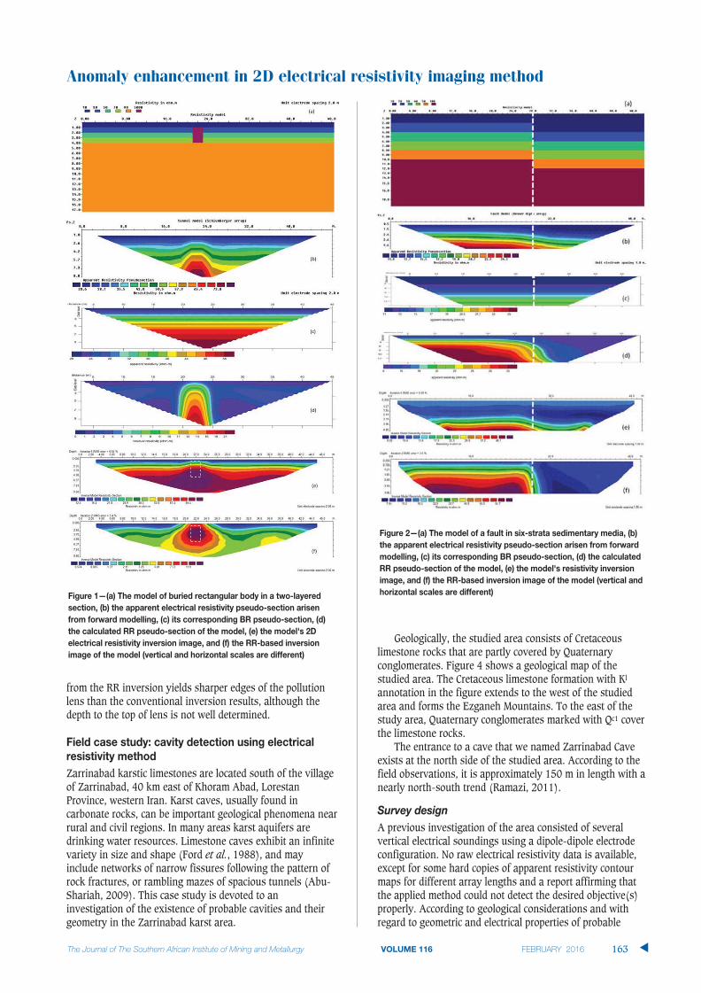
Anomaly enhancement in 2D electrical resistivity imaging method
163 �
from the RR inversion yields sharper edges of the pollutionlens than the conventional inversion results, although thedepth to the top of lens is not well determined.
Zarrinabad karstic limestones are located south of the villageof Zarrinabad, 40 km east of Khoram Abad, LorestanProvince, western Iran. Karst caves, usually found incarbonate rocks, can be important geological phenomena nearrural and civil regions. In many areas karst aquifers aredrinking water resources. Limestone caves exhibit an infinitevariety in size and shape (Ford et al., 1988), and mayinclude networks of narrow fissures following the pattern ofrock fractures, or rambling mazes of spacious tunnels (Abu-Shariah, 2009). This case study is devoted to aninvestigation of the existence of probable cavities and theirgeometry in the Zarrinabad karst area.
Geologically, the studied area consists of Cretaceouslimestone rocks that are partly covered by Quaternaryconglomerates. Figure 4 shows a geological map of thestudied area. The Cretaceous limestone formation with Kl
annotation in the figure extends to the west of the studiedarea and forms the Ezganeh Mountains. To the east of thestudy area, Quaternary conglomerates marked with Qc1 coverthe limestone rocks.
The entrance to a cave that we named Zarrinabad Caveexists at the north side of the studied area. According to thefield observations, it is approximately 150 m in length with anearly north-south trend (Ramazi, 2011).
A previous investigation of the area consisted of severalvertical electrical soundings using a dipole-dipole electrodeconfiguration. No raw electrical resistivity data is available,except for some hard copies of apparent resistivity contourmaps for different array lengths and a report affirming thatthe applied method could not detect the desired objective(s)properly. According to geological considerations and withregard to geometric and electrical properties of probable

Anomaly enhancement in 2D electrical resistivity imaging method
cavities in the area, a combined resistivity sounding andprofiling electrode array (CRSP) was applied. CRSP wasintroduced by Ramazi (2005) and is defined as follows: threevertical electrical soundings are surveyed simultaneously by aset of measurement current electrodes that are normally usedfor one vertical electrical sounding (VES). In this array thedistance of each measuring station is equal to the spacing ofthe potential electrodes (see Figure 5 for a schematicrepresentation of the CRSP array). As shown in the figure,CRSP is similar to the Schlumberger and Wenner-Schlumberger arrays in central measurements; however, thepotential electrode spacing can be decreased for shortercurrent electrode distances and hence increased horizontalresolution obtained. The potential electrode spacing dependson the survey objectives, including the depth of investigation.We define n as:
where AB is the current electrode spacing and Pc is theappropriate potential electrode spacing (P2P3 distance), which
is equal to PL and PR. The first current electrode spacing inroutine CRSP measurements starts at n=2, which is equal tofive times the appropriate potential electrode spacing(including the measuring station interval). For example, ifthe measuring stations interval is 5 m (P1P2 = P2P3 = P3P4 = 5 m), the first current electrode spacing (AB) for CRSPmeasurements will be 25 m (AB = 25 m). AB is increased forthe other measurements as the following:
For n=1 the current electrode distance is equal to threetimes the potential electrode spacing (for example AB = 15m); in this case and also for other near surface measurements(AB<15 m), each the sounding points is surveyedindividually as in the Schlumberger array. The data obtainedby this array could be processed and interpreted as soundingcurves and/or into pseudo-sections. As seen in Figure 5, theCRSP array has the advantage of penetrating deep in thesubsurface as well as detecting lateral changes through theacquisition of more data in a section. In practice, CRSP hasbeen successfully applied to different mineral exploration andengineering site investigations (Ramazi and Mostafaie,2013). It should be noted that a combined method, called‘combined sounding-profiling resistivity’ was also proposedby Karous and Pernu (1985). This method is significantlydifferent from CRSP in electrode configuration, fieldoperation, and processing. For example, in the Karous and
�
164

Pernu proposed array, the distance between potentialelectrodes is constant, but in the CRSP configuration, threecouples of potential electrodes are used (PL, PC, and PR).Likewise, the Karous and Pernu configuration is based on athree-electrode array, while a symmetrical array is used inthe CRSP method (Ramazi and Jalali, 2014).
In this case study, CRSP resistivity measurements wereacquired along three survey lines. Figure 6 shows thelocations of designated survey lines. Each profile wasapproximately 600 m in length and the distance between twosurvey lines was set to 30 m. In total, 19 stations (with 57measurement points) were acquired along each survey line.In all survey lines the measuring point interval as well aspotential electrode spacing was assigned as 10 m. Currentelectrode distances (AB) were selected from 50 m to 250 m.For AB lengths shorter than 50 m, the distance of eachcouple of the potential electrodes was decreased to 5 m, andeach of the sounding points was surveyed separately (n=1).
The RR technique was applied to the acquired data asdescribed above. Figure 7 shows the VES resistivity curvealong station 4 of survey line P1. The BR function wascalculated using the VES data from station 4 as follows:
[2]
where BR is the background resistivity value of eachmeasuring point and x is the corresponding current electrodespacing (AB).
Figure 8(a) illustrates the apparent resistivity pseudo-section along survey line P1, while Figure 8(b) shows itscorresponding BR pseudo-section. The RR pseudo-sectionalong survey line P1 is shown in Figure 8(c). Figure 8(d)illustrates the conventional resistivity inversion along surveyline P1. As seen from the figure, the formation consists ofseveral resistivity layers that increase in resistivity withdepth.
Figure 8(e) shows the RR-based inversion image alongP1. The figure shows that by applying the RR method, the
rbackground resistivity layers reduce to a relatively moreuniform background; moreover, anomalies with high RRvalues show potential karst cavities (see Table I). Thepositions of the RR anomalies are also shown in theconventional inversion image in Figure 8(d). According toprevious observations, point C represents the ZarrinabadCave footprint. A comparison between Figure 8(d) and Figure8(e) clearly shows that the anomalies are considerably moreenhanced in the RR-based image. Drill testing into areas Aand E convincingly proved the results.
Anomaly enhancement in 2D electrical resistivity imaging method
165 �

Anomaly enhancement in 2D electrical resistivity imaging method
Figure 9(a) shows the apparent resistivity pseudo-sectionalong survey line P2, while Figure 9(b) shows itscorresponding BR pseudo-section. The RR pseudo-sectionalong survey line P2 is shown in Figure 9(c). Figure 9(d)represents the electrical resistivity inversion image alongsurvey line P2, while Figure 9(e) shows its correspondingRR-based inversion image. The background resistivity layersin Figure 9(d) were removed in Figure 9(e). Area D in thefigure shows the footprint of Zarrinabad Cave. Areas A and Hin Figure 9(e) represent RR anomalous zones that wereconcealed by the natural regional resistivity gradient inFigure 9(d). Table II describes anomalies detected in thefigure.
The apparent resistivity pseudo-section along surveyline P3 is shown in Figure 1(a), while Figure 10(b) shows its
corresponding BR pseudo-section. Figure 10(c) alsoillustrates the RR pseudo-section along survey line P3. Figure 10(d) shows the electrical resistivity inversion imagealong survey line P3, and Figure 10(e) represents itscorresponding RR-based inversion image. A visualcomparison of Figure 10(d) and Figure 10(e) highlights theproficiency of the RR technique well. The RR anomalouszones of areas C, D, E, and F in Figure 10(e) completelydistinguish shallow karst zones, their extensions, andprobable connections. Further drilling into area D proved thisinterpretation. Areas E and F in Figure 10(e) representZarrinabad Cave footprints. Areas A, B, C, G, and H in Figure10(e) represent several anomalous RR zones, which arefaded in the conventional electrical resistivity inversion image(Figure 10(d)), suggesting filled or small cavities. Thisinterpretation has not been drill-tested (Table III).
In this paper the residual resistivity (RR) technique was
introduced as a new method of electrical resistivity dataprocessing. The RR technique can enhance probable localanomalies through the elimination of regional resistivitygradients. The technique may highlight positive and/or
�
166
Table II
Description of the anomalies detected in Figure 9(e)
Anomaly Interpretation Local X-coordination (m) Predicted depth (m) Actual depth (m)
A Karst zone 110 Z ≥15 Z ≥15B Fractured zone 210 Z ≥8 N/AC Small cavity 330 6-8 N/AD Zarrinabad Cave 380 8-12 ~12E Karst zone 410 Z ≥15 N/AF Cavity 430 12 ≥ Z ≥8 N/AG Fractured zone 470 Z ≥7 ≥7H Karst zone 500 Z ≥7 N/AI Karst zone 580 Z ≥15 N/A
Table I
Description of anomalies detected in Figure 8(e)
Anomaly Interpretation Local X-coordination (m) Predicted depth (m) Actual depth (m)
A Karst zone 110 Z ≥15 Z ≥ 14B Karst zone 300 Z ≥8 N/AC Zarrinabad Cave 340 8-12 ~13D Shallow cavity 390 5-8 N/AE Karst zone 440 Z ≥8 Z ≥10F Karst zone 470 Z ≥10 N/AG Karst zone 490 Z ≥8 N/AH Fractured zone 550 Z ≥12 N/A

negative anomalies representing materials with electricalresistivity values more or less than the background levelrespectively. The most important conclusions are summarizedas follows:
� Background resistivity plays an important role inresistivity anomaly detection. In many cases it changesdue to variations in physical properties of theinvestigated area (as in the synthetic and field casestudies)
� The existence of potentially fictitious anomalies isreduced by the RR technique due to the determinationof the background resistivity gradient for eachmeasuring point. Likewise, probable anomalies that arenot easily detectable by conventional inversion
methods are highlighted with acceptable precision andresolution
� Shallow and deep underground cavities were detectedin the Zarrinabad karst area by applying the RRtechnique. Further drilling convincingly proved theresults obtained by this technique
� The CRSP (combined resistivity sounding and profiling)electrode array is an appropriate array for applying theRR technique.
ABU-SHARIAH MOHAMAD, I.I. 2009. Determination of cave geometry by using ageoelectrical resistivity inverse model. Engineering Geology, vol. 105. pp. 239–244.
AIZEBEOKHAI, A.P., OLAYINKA, A.I., and SINGH, V.S. 2010. Application of 2D and3D geoelectrical resistivity imaging for engineering site investigation in acrystalline basement terrain, southern Nigeria. Environmental EarthSciences, vol. 61. pp. 1481–1492.
BAYRAK, M. AND SENEL, L. 2012. Two-dimensional resistivity imaging in theKestelek boron area by VLF and DC resistivity methods. AppliedGeophysics, vol. 82. pp. 1–10.
CANDANSAYAR, M.E. and BASOKUR, A.T. 2001. Detecting small scale targets bythe 2D inversion of two-sided three-electrode data: application to anarcheological survey. Geophysical Prospecting, vol. 49, no. 1. pp. 13–25.
DE LA VEGA, M., OSELLA, A., and LASCANO, E. 2003. Joint inversion of Wennerand dipole-dipole data to study gasoline-contaminated soil. AppliedGeophysics, vol. 54. pp. 97–109.
FEHDI, C., BAALI, F., BOUBAYA, D., and ROUABHIA, A. 2011. Detection of sinkholesusing 2D electrical resistivity imaging in the Cheria Basin (north-east ofAlgeria). Arabian Journal of Geosciences, vol. 14, no. 1-2. pp. 181–187.
FORD, D.C., PALMER, A.N., and WHITE, W.B. 1988. Landform developments;karst. The Geology of North America. Vol. O-2, Hydrogeology. pp. 401–412.
HA, H.S., KIM, D.S., and PARK, I.J. 2010. Application of electrical resistivitytechniques to detect weakand fracture zones during undergroundconstruction. Environmental Earth Sciences, vol. 60. pp. 723–731.
LOKE, M. 1995-2013. RES2DMOD, 2D resistivity and IP forward modeling, Ver.3.0. www.geotomosoft.com/r2dmodwin.zip [Accessed 12 June 2014].
LOKE, M. and BARKER, R. 1996. Rapid least squares inversion of apparentresistivity pseudo-sections using a quasi Newton's method. GeophysicalProspecting, vol. 44. pp. 131–152.
KAMKAR-ROUHANI, A. 1998. Development and application of processingtechniques for signal enhancement using multisystem resistivitymeasurements. PhD thesis, Curtin University of Technology, Australia.
KAROUS, M. and PERNU, T.K. 1985. Combined sounding-profiling resistivitymeasurements with the three-electrode arrays. Geophysical Prospecting,vol. 33. pp. 447–459.
Anomaly enhancement in 2D electrical resistivity imaging method
167 �
Table III
Description of the anomalies detected in Figure 10(e)
Anomaly Interpretation Local X-coordination (m) Predicted depth (m) Actual depth (m)
A Fractured zone 60 Z ≥8 N/AB Fractured zone 100 Z ≥10 N/AC Fractured zone 300 Z ≥12 N/AD Karst zone 360 Z ≥15 Z ≥13E Zarrinabad Cave 400 8-12 14F Cavity 430 Z ≥8 12-14G Karst zone 500 Z ≥18 N/AH Fractured zone 570 Z ≥13 N/A

Anomaly enhancement in 2D electrical resistivity imaging method
NIWAS, S.M. and MEHROTRA, A.M. 1997. A stable iterative scheme for inversionof direct current resistivity sounding data. Acta Geodaetica et GeophysicaHungarica, vol. 32, no. 1-2. pp. 15–25.
NORDIANA, M.M., ROSLI, S., and NAWAWI, N.N.M. 2014. A numerical comparisonof enhancing horizontal resolution (EHR) technique utilizing 2Dresistivity imaging. Arabian Journal of Geosciences, vol. 17, no.1. pp. 299–309.
OLDENBURG, D.W. and LI, Y. 1994. Inversion of induced polarization data.Geophysics, vol. 59. pp. 1327–1341.
Papadopoulos, N.G., Tsokas, G.N., Dabas, M., Yi, M. and Tsourlos, P. 2009. 3Dinversion of Automated Resistivity Profiling (ARP) data. ArcheoSciences,vol. 33 (suppl.). pp. 329–332.
RAMAZI, H.R. 2005. Combined resistivity sounding and profiling and itsapplication in mineral exploration and site investigation. Technical report.Zamin Moj Gostar, Tehran, Iran. 21 pp. (in Persian).
RAMAZI, H.R. 2011. Zarrinabad karsts geophysical report. Zamin Moj Gostar,Tehran, Iran. 100 pp. (in Persian).
RAMAZI, H.R. and JALALI, M. 2014. Contribution of geophysical inversion theoryand geostatistical simulation to determine geoelectrical anomalies. StudiaGeophysica et Geodaetica, vol. 59, no. 1. pp. 97–112. DOI:10.1007/s11200-013-0772-3
RAMAZI, H.R. and MOSTAFAIE, K. 2013. Application of integrated geoelectricalmethods in Marand (Iran) manganese deposit exploration. ArabianJournal of Geosciences, vol. 6, no. 8. pp. 2961–2970.
SMITH, N.C. and VOZZOF, K. 1984. Two dimensional DC resistivity inversion fordipole- dipole data. IEEE Transactions on Geosciences and RemoteSensing, vol. GE-22, no. 1. pp. 21–28.
WILKINSON, P. B., MELDRUMM, P.I., KURAS, O., CHAMBERS, J.E., HOLYOAKE, S.J., andOGILVY, R.D. 2010. High-resolution electrical resistivity tomographymonitoring of a tracer test in a confined aquifer. Applied Geophysics, vol. 70. pp. 268–276.
YILMAZ, S. and NARMAN, C. 2014. 2-D electrical resistivity imaging forinvestigating an active landslide along a ridgeway in Burdur region,southern Turkey. Arabian Journal of Geosciences. DOI: 10.1007/s12517-014-1412-0. �
�
168
9–10 June 2016 • Mintek, Randburg
Driving mining productivity improvement through technology and innovation
For further information contact:Conference Co-ordinator, Camielah JardineSAIMM, P O Box 61127, Marshalltown 2107
Tel: (011) 834-1273/7Fax: (011) 833-8156 or (011) 838-5923
E-mail: [email protected]: http://www.saimm.co.za
BACKGROUNDThe South African mining industry finds itself at a crossroadswhere current levels of productivity and safety, which are drivenby current mining methods, will no longer be either socially or eco-nomically acceptable.
The future competitiveness of the Southern African mining in-dustry depends on the application of appropriate and workabletechnologies, as well as innovative mining methods, that improvesafety and productivity. These will be based on process based or-ganisations that are enabled and empowered by increasing levelsof real time data and information integrated across the value chain.
This event is aimed at presenting examples of how technologycan improve the costs and competiveness of the SA Mining indus-try, within the next 10 years and technology that is in use now. Not
only will it draw on case studies and examples of technology de-velopment, but it will also explore innovative ways of applying stateof the art technologies from other sectors, to the mining environ-ment.
OBJECTIVES
To showcase, explain and demonstrate the potential for opera-tional improvement through innovative but practical technologicalsolutions aimed at improvements in quality, output and productiv-ity.
It is also aimed at achieving a common vision of ‘the art ofthe possible’ as well as exploring new paradigms for mining in thefuture.

Low-grade, medium-rank C bituminous coalsare mined for South African chemicalcompanies from six different collieries in theHighveld coalfield, located in the MpumalangaProvince of South Africa (Pinheiro et al.,1998–1999). Products containing coarse coalparticles mixed with rock fragments (> 6 mmcoal fraction) are transported from the minesources to the preparation plant, where theyare blended according to their availability toform a mixture that is suitable for thecompany’s coal conversion operations (Matjieet al., 2006; van Dyk et al., 2006). Finer coal
particles are pulverized to 100% passing 75 m and combusted in boilers to produceenergy or electricity for the domestic powerand chemical industries (van Alphen, 2005).
As discussed further by authors such asBenson (1987), Ward (2002), and van Alphen(2005), the material regarded as mineralmatter in coal consists effectively of twofractions: (1) a range of discrete crystallinemineral particles occurring in the coal indifferent ways, and (2) a range of non-mineralinorganic elements dissolved in the pore wateror intimately associated with the organicmatter (Li et al., 2007, 2010; Mares et al.,2012). Along with other constituents such asorganic sulphur, the mineral matter is the mostsignificant factor in problems that may beassociated with coal handling and use, such asabrasion, stickiness, slagging, sintering,corrosion, and pollution (Falcone et al., 1984;Tangsathitkulchai, 1986; Bryers, 1996; Guptaet. al., 1996; Wall et al., 2002; Creelman et al.,2013; Su et al., 2001; Barnes, 2009; Matjie etal., 2008, 2011, 2012a, 2012b). In addition,mineral matter occurring within the coalmacerals, especially the non-mineral inorganicelements, is a key contributor to the formationof ultrafine ash particles, as well as condensedmetallic vapours, during coal combustion(Buhre et al., 2006; Zhang, 2006).
Determination of mineral matter andelemental composition of individualmacerals in coals from Highveld minesby R.H. Matjie*, Z. Li†‡, C.R. Ward†, J.R. Bunt*, and C.A. Strydom**
A number of conventional and advanced analytical techniques (proximateand ultimate analysis, low-temperature oxygen-plasma ashing, X-raydiffraction, X-ray fluorescence spectrometry, coal petrography, and light-element electron microprobe analysis) have been integrated and cross-checked to provide detailed characterization of coals from the Highveldcoalfield in South Africa, as a basis for better understanding of themineralogical and chemical properties of the individual coal sources thatare blended as feedstocks for combustion and carbon conversionprocesses. The techniques included methods to quantify the abundanceand composition of the mineral matter (minerals and non-mineralinorganic elements), and also the abundance and chemical composition ofthe individual macerals in the individual coals concerned.
Kaolinite is the most abundant of the minerals in the coals studied,with lesser but still significant proportions of quartz, mica and/or illite,dolomite, calcite, and pyrite. Small but variable proportions of anatase,goyazite, and siderite are present in some coal samples. Electronmicroprobe analysis, based on a special configuration for light-elementstudy, shows that the vitrinite contains less carbon and more oxygen, andhas significantly higher concentrations of nitrogen and organic sulphur,than the inertinite macerals in the same samples. Minor proportions oforganically-associated inorganic elements, including titanium, were alsoidentified in some of the maceral components.
A comprehensive knowledge of the minerals and non-mineralinorganic elements in the coals used for feedstock preparation, obtained byintegration of data from these advanced analytical techniques with moreconventional analyses, may be of benefit in understanding the processesthat take place during coal utilization, and also in avoiding or amelioratingsome of the operational and environmental problems that may occur indifferent sectors of the coal utilization industry.
coal analysis, coal petrology, mineral matter, X-ray diffraction, electronmicroprobe.
* Unit for Energy and Technololgy Systems, Schoolof Chemical and Minerals Engineering, North-West University, Potchefstroom.
†‡ School of Biological, Earth and EnvironmentalSciences, University of New South Wales, Sydney,Australia, and CSIRO Energy Flagship, NorthRyde, Australia.
** School of Physical and Chemical Sciences, North-West University, Potchefstroom.
© The Southern African Institute of Mining andMetallurgy, 2016. ISSN 2225-6253. Paperreceived Jul. 2015; revised paper received Aug. 2015.
169 �
http://dx.doi.org/10.17159/2411-9717/2016/v116n2a8

Determination of mineral matter and elemental composition of individual macerals
�
170
The inorganic elements within the organic structure ofcoal macerals may react in a different way to the sameelements occurring in the discrete mineral particles (Falconeet al., 1984; Ward, 2002). More specifically, Quann andSarofim (1986) found that the organically-associatedinorganic elements (calcium and magnesium) in lignitic coalreact with free aluminium silicate to form fused agglomeratesduring combustion.
Many of the minerals in coal undergo chemical andcrystallographic changes at the temperatures associated withcombustion (O’Gorman and Walker, 1973; Vassilev et al.,1995; Creelman et al., 2013), including during preparation oflaboratory ash samples for conventional (proximate) analysisprocedures. The minerals in a coal sample are thereforeusually isolated and identified by low-temperature oxygen-plasma ashing (Gluskoter, 1965; Standards Australia, 2000),during which the coal is exposed, under vacuum, to a streamof electronically activated oxygen, which destroys the organicmatter at a temperature of around 120°C, leaving a residueconsisting of the essentially unaltered mineral components.The organic sulphur in the coal macerals may, however,interact with organically-associated inorganic elements toform mineral artefacts in the plasma-ashing process (Frazerand Belcher, 1973). Non-mineral calcium, for example, mayreact with sulphur released from the coal to form bassanite(CaSO4.½H2O) in the low-temperature ash residues of SouthAfrican coal samples (Matjie et al., 2008, 2011, 2012a,2012b; Hlatshwayo et al., 2009). The formation of suchcalcium sulphate artefacts provides an example of the greaterreactivity shown by non-mineral inorganic elements duringcoal combustion, relative to equivalent or counterpartelements (e.g. calcium in calcite) occurring in less reactivemineral forms.
Several authors (e.g. Raymond and Gooley, 1978; Raymond,1982; Clark et al., 1984; Ward and Gurba, 1998) have usedelectron microprobe analysis and similar techniques todetermine the concentration of organic sulphur in coalmacerals. In practical terms this represents sulphur thatcannot be removed from the coal, even if the pyrite and othersulphur-bearing phases are completely separated out byconventional preparation techniques (Ryan and Ledda,1997).
As an extension of this approach, special light-elementelectron microprobe techniques have been used to determinethe percentages of carbon, oxygen, and nitrogen in theindividual macerals of coal samples (e.g. Bustin et al., 1993;Mastalerz and Gurba, 2001; Ward et al., 2005, 2007, 2008),providing a better understanding of the differences betweenthe individual components of the organic matter tocomplement more conventional chemical and petrographicstudies. This approach has also provided new insights intothe occurrence of non-mineral inorganic elements, such asCa, Mg, Fe, and Al, in the different coal macerals and thechanges that may take place in those elements withadvancing rank (Li et al., 2007, 2010).
The minerals and other inorganic elements in coal mayinteract with each other when the coal is used. The nature of
these interactions and the impact of the associated productsdepend on the minerals involved, and also on factors such asthe utilization conditions (e.g. temperature,oxidation/reduction), the mode(s) of mineral or elementoccurrence within the coal, and the opportunities for andduration of contact between the various phases in theutilization system (e.g. Bryers, 1996; Grigore et al., 2008;Matjie et al., 2011, 2012a, 2012b; Creelman et al., 2013).
In order to manage these processes and minimize theirpotentially adverse effects, it is important to have a goodunderstanding of the chemical and mineralogical properties ofthe individual coals that contribute to the feedstockpreparation, especially the nature and mode of occurrence ofthe different mineral matter components. Although asignificant amount of information is available from chemicalanalyses (e.g. proximate analysis, ultimate analysis, ashanalysis), and mineralogical analysis has also been carriedout on some South African coals (Pinheiro et al., 1998-1999;Gaigher, 1980; DME, 2006; Pinetown et al., 2007; Matjie etal., 2011), very little information is available on the chemicalcomposition of the actual macerals in South African coals oron the mineralogical composition of low-temperature ashresidues isolated from South African coal samples.
The objective of this paper is to describe the application oftwo advanced analytical techniques – evaluation of mineralmatter by quantitative X-ray diffraction and chemicalanalysis of coal macerals using the electron microprobe – tosome industrially significant South African coals. As well asdescribing the techniques and the results obtained, the studyincludes comparisons with data from other, moreconventional procedures, partly to check and confirm theresults obtained and partly to illustrate the relation betweenthe information from the advanced techniques andconventional coal analysis data. The use of such informationin understanding the behaviour of South African coals duringutilization is also included in the discussion.
Samples of coal from six different mines in the Highveldcoalfield were analysed. Each coal represents a component ofthe blend used for gasification and/or combustionapplications in the Sasol industrial complex. Representativeportions of each sample were crushed to the appropriateparticle size and submitted to laboratories in South Africaand Australia for the analysis programme described below.
Representative portions of each coal were ground to 100%passing 212 m, and the ground samples were analysed byproximate analysis, using standard methods to measure thepercentages of moisture (SABS 924, ISO 589), ash (ISO1171), and volatile matter (ISO 562). Ultimate analysis of thecoals was carried out using the ASTM D5373 procedure. TheASTM D4239 method was used to determine the totalsulphur content. The overall results were expressed to a dryash-free (daf) basis, and the oxygen content was calculatedby difference.
Other portions of each coal were ground to fine powderand ashed at 815°C at the University of New South Wales inSydney, Australia. The ashes were fused with lithiummetaborate and cast into glass discs, following the method of

Determination of mineral matter and elemental composition of individual macerals
171 �
Norrish and Hutton (1969). The discs were analysed by X-ray fluorescence (XRF) spectrometry using a Philips PW 2400spectrometer and SuperQ software, and the results wereexpressed as percentages of the major element oxides in eachash sample.
Representative splits of each crushed coal were mixed withepoxy resin and prepared as polished sections forpetrographic analysis. Petrographic analysis was carried outby Coal and Organic Petrology Services Pty Ltd, Sydney,Australia, based on optical microscopy using oil-immersionobjectives. The procedure followed Australian StandardAS2856, based on ICCP guidelines and ISO 7404. Thevolumetric proportions of individual macerals and maceralgroups, and also of the visible mineral components, weredetermined for each of the coals, as well as the meanmaximum reflectance of the vitrinite in the coal samples.
Other representative splits of each coal sample were finelypowdered, and a representative portion of each powdersubjected to low-temperature oxygen-plasma ashing using anIPC four-chamber asher at the University of New SouthWales, as outlined in Australian Standard 1038, Part 22. Themass percentage of low-temperature ash (LTA) wasdetermined in each case.
The mineralogy of each LTA from the coal was analysedby X-ray powder diffraction (XRD) using a Phillips X'pertdiffractometer with Cu K radiation, and the minerals presentidentified by reference to the International Center forDiffraction Data (ICDD) Powder Diffraction File. Quantitativeanalyses of mineral phases in each LTA were made usingSiroquant™, a commercial XRD interpretation softwarepackage originally developed by Taylor (1991) based on therefinement principles described by Rietveld (1969).
The clay fraction (less than 2 m effective diameter) ofeach LTA sample was isolated by ultrasonic dispersion insodium hexametaphosphate (Calgon) and subsequentsettling. This fraction was concentrated, mounted on glassslides, and investigated in more detail by XRD of theresulting oriented aggregates using glycol and heat treatment(Hardy and Tucker, 1988). The relative proportions of thedifferent clay minerals in this fraction for each sample weredetermined using the method described by Griffin (1971).
Polished sections of representative coal fragments(approximately 5 mm diameter) were prepared from eachsample. The fragments were selected to embrace the range ofmacerals in each sample, as indicated by the macroscopicappearance (lithotype) of the coal in each case.
The surfaces of the polished sections were coated with athin film of carbon, and loaded into a Cameca SX-50 electronmicroprobe analyser at the University of New South Wales,equipped with the Windows®-based SAMx operating systemand interface software. The elemental chemistry of theindividual macerals in each sample was analysed on thisinstrument using special light-element techniques, followingprocedures described more fully by Bustin et al. (1993) andWard et al. (2005).
Images were also captured of selected fields of view foreach sample (Figure 1) using the optical observation systemof the microprobe unit. Although the resolution was less thanthat obtained by reflected-light microscopy under oilimmersion and some details were obscured by the carboncoating, the light optics of the microprobe were found to beadequate for recognition of the individual macerals, basedmainly on shape and other textural features.
Individual points on representatives of the differentmaceral groups were analysed for each sample using theoperating conditions described by Ward et al. (2005). Theaccelerating voltage for the electron beam was 10 kV and thefilament current 20 nA, with a magnification of 20 000×,giving an beam spot size on the sample of around 5 to 10 min diameter. As discussed by Bustin et al. (1993), anindependently analysed anthracite sample was used as thestandard for carbon in the analysis process. A range ofmineral standards was used for the other elements (Li et al.,2010).
The percentages of carbon, oxygen, nitrogen, sulphur,silicon, aluminium, calcium, magnesium, potassium,titanium, and iron were measured for each selected point,with a note on the type of maceral represented in each case.The results of the individual analyses were tabulated inspreadsheet format. Although care was taken to analyse only’clean’ macerals and avoid areas where visible minerals werealso present, the area analysed for some points unavoidablyincluded significant proportions of mineral components (e.g.

Determination of mineral matter and elemental composition of individual macerals
quartz, clay, and pyrite) as well as the organic matter. Pointsthat apparently included mineral contaminants (e.g. pointswith high (>0.5%) Si or with particularly high percentages ofboth Fe and S) were excluded from consideration; so, too,were points that included some of the mounting epoxy resin(e.g. epoxy filling empty cell structures), indicated byunusual oxygen and high nitrogen contents.
Proximate analysis data (Table I) shows that the samplesyield 30–34% volatile matter on a daf basis. The inherentmoisture content of the coals ranges between 2.9% and 3.8%,and the ash yield of the samples tested (air-dried basis)ranges between 22.1% and 29.7%. Total sulphur content,determined as part of the ultimate analysis procedure (seebelow) ranges from 0.7% to 1.1% when expressed on an air-dried basis.
Ultimate analysis data (Table II) indicates that the coalscontain high proportions of carbon (77–80% daf), withrelatively low concentrations of total sulphur (0.9–1.6% daf),nitrogen (2-2.1% daf), and hydrogen (4.0–4.6% daf). Theoxygen content of the coals (daf basis) was found bycalculation to range from 12 to 16%.
The proportions of inorganic elements (reported as oxides) in the coal ashes, derived from XRF analysis, are given inTable III. The percentage of ash for each sample analysed inthis way, determined as part of the XRF analysis procedure,is also indicated. These percentages are slightly differentfrom the ash percentages in Table I, partly because ofdifferences in the samples actually analysed by the twolaboratories, and also possibly because of differences insulphur retention within the ashes due to different ashpreparation techniques.
Silica (SiO2, 47–58%) and alumina (Al2O3, 21–28%) arethe dominant constituents in the coal ashes, with lesser butstill significant proportions of CaO, Fe2O3, MgO, and TiO2.Other oxides, with the exception of SO3 and in some casesP2O5 and K2O, each make up less than 1% of the coal ashsamples.
The percentage of sulphur retained as SO3 in the ash isless than that expected if all of the sulphur in the coal (thetotal sulphur in Table I) was retained in this way. As with theformation of bassanite in oxygen-plasma ash discussedabove, the extent of sulphur retention depends partly on theashing conditions (e.g. heating rate) and partly on theproportion of elements such as Ca that are available tocombine with the S released from the coal during the ashingprocess. For example, the lowest percentage of SO3 in Table III occurs in sample 2, which also has the lowestpercentage of CaO, and the highest SO3 percentage occurs insample 6, which has the highest CaO percentage. Linksbetween CaO and SO3 in ashes prepared under similarconditions are discussed further by Koukouzas et al. (2009).
Petrographic analysis (Table IV) indicates that the coals areinertinite-rich, with significant proportions (9–27%) of visiblemineral matter. If the minerals are excluded and the maceralpercentages recalculated to 100%, the coals contain 19–30%vitrinite and 64–77% inertinite components on a mineral-freebasis. Liptinite makes up between 3 and 5% (mineral-free) ofthe coal samples. Samples 5 and 6 contain slightly higherproportions of vitrinite and liptinite and lower proportions ofinertinite than the other coal samples.
The vitrinite in the coals is represented mainly byrelatively thick bands of collotelinite (telocollinite). Finerbands of collodetrinite (desmocollinite) occur in minorproportions, typically as a structureless matrix containingother maceral components. The principal inertinite maceral issemifusinite, with minor proportions of inertodetrinite,
�
172
Table I
Proximate analysis data (air-dried basis) for thecoals tested
Sample number 1 2 3 4 5 6
Moisture (%) 3.3 2.9 3.2 3.4 3.0 3.8Ash (%) 24.5 29.0 29.7 27.2 26.8 22.1Volatile matter (%) 21.7 22.9 21.3 21.5 22.4 23.1Fixed carbon (%) 50.5 45.2 45.8 47.9 47.8 51.0Total sulphur (%) 1.1 1.0 0.8 1.0 1.1 0.7Volatile matter (daf basis, %) 30.1 33.6 31.7 31.0 31.9 31.2
Table II
Ultimate analysis data for the coals tested (dry,ash-free basis)
Sample number 1 2 3 4 5 6
Carbon (%) 79.9 78.5 77.1 77.8 79.0 77.9Hydrogen (%) 4.36 4.55 4.07 4.12 4.59 4.29Nitrogen (%) 2.12 2.00 1.97 2.00 2.08 2.00Total sulphur (%) 1.55 1.41 1.15 1.50 1.62 0.92Oxygen (% by difference) 12.1 13.5 15.7 14.6 12.7 14.9
Table III
Inorganic oxide percentages (wt%) from XRFanalysis of coal ash samples
Sample number 1 2 3 4 5 6
Ash (815°C) 28.9 40.6 30.8 32.8 30.6 22.8SiO2 51.27 53.67 52.17 49.63 58.25 46.79Al2O3 24.70 27.95 26.40 27.05 21.22 23.71Fe2O3 4.31 3.69 2.46 3.55 3.48 3.74TiO2 1.24 1.29 1.54 1.48 1.15 1.43P2O5 0.40 .070 0.67 0.83 0.70 1.17CaO 7.46 5.70 8.08 7.75 6.19 13.27MgO 2.19 1.67 2.64 2.11 1.70 3.64Na2O 0.41 0.22 0.50 0.36 0.38 0.55K2O 0.79 1.13 0.84 1.21 1.07 0.35SO3 5.57 4.50 4.94 5.59 4.47 6.13Total 98.33 100.52 100.24 99.56 98.60 100.78

macrinite, and fusinite, and traces of micrinite are alsopresent. Sporinite and cutinite are the only liptinite maceralspresent, with sporinite being especially abundant in theliptinite-rich coals represented by samples 5 and 6.
The minerals or mineral-rich components visible underthe microscope are mainly disseminated clays, with minorcarbonate and traces of quartz and pyrite. Stony particles(shale) are also present in the crushed coal grain mounts,especially in the mineral-rich coal of sample 2. It should benoted that the percentages in Table IV are all volumepercentages; since minerals such as quartz and clays typicallyhave densities around twice those of the macerals in coal, theweight percentages of mineral material would be significantlyhigher, as a fraction of the coal, than the volume percentagesindicated in the table.
The coals have a mean maximum vitrinite reflectance,measured on collotelinite (telocollinite), of 0.70–0.75%.According to ISO 11760 (ISO, 2005), this indicates that thecoals can be classified as medium-rank C bituminous coals.
Table V summarizes the weight percentage of LTA isolatedfrom the coals by oxygen-plasma ashing, and also thepercentages of the individual minerals in each LTA, based onthe powder XRD and Siroquant evaluations. Figure 2illustrates typical X-ray diffractograms of the LTA from thecoal samples.
Figure 3A provides a plot of the LTA percentage for eachsample against the percentage of high-temperature (815°C)ash indicated for the same coal sample in Table III. The plotincludes a diagonal line, along which the data points wouldbe expected to fall if both percentages were equal. The datapoints, however, fall above this equality line, indicating thatthe percentages of mineral matter, expressed by the LTA, areslightly higher than the high-temperature ash yields from thesame coal samples. This is because the LTA contains anabundance of essentially unaltered minerals, such as clayminerals, pyrite, and carbonates, which liberate volatilecomponents and leave a lesser proportion of altered mineralresidue after the high-temperature ashing process. Forexample, although quartz is non-reactive, kaolinite losesaround 14% by mass and calcite loses around 44% on high-temperature ashing, due to dehydroxylation anddecarbonization reactions respectively. The slope factor(1.08) in the linear regression equation indicates that, onaverage, the overall proportion of mineral matter (LTA) in thecoal samples is typically around 8% higher than the (high-temperature) ash yield.
Determination of mineral matter and elemental composition of individual macerals
173 �
Table IV
Petrographic analysis of coal samples (vol.%)
Maceral group 1 2 3 4 5 6
A – Minerals includedVitrinite (%) 16.7 18.9 17.4 17.2 26.7 24.7Liptinite (%) 3.0 2.7 2.7 2.8 4.7 4.9Inertinite (%) 67.2 51.8 64.9 63.7 55.7 61.6Minerals (%) 13.1 26.6 15.0 16.2 12.8 8.8
B – Mineral-freeVitrinite (%) 19.2 25.8 20.5 20.6 30.6 27.1Liptinite (%) 3.5 3.7 3.2 3.4 5.4 5.4Inertinite (%) 77.3 70.6 76.3 76.1 63.9 67.5Rvmax (%) 0.72 0.70 0.75 0.72 0.70 0.7
Table V
Mineralogy (wt%) of LTA from coal samples frompowder XRD analysis
Sample number 1 2 3 4 5 6
LTA 31.9 43.9 34.5 36.2 33.6 24.6Quartz 17.6 21.5 20.6 15.2 20.1 18.3Kaolinite 51.4 50.4 49.5 44.0 50.8 47.6Illite bld 5.7 bld 5.7 5.3 2.2Mica 10.4 7.4 7.0 6.9 4.5 4.5Calcite 2.1 1.2 2.7 9.8 1.8 4.6Dolomite 10.3 6.4 11.7 10.0 10.2 15.2Siderite bld 1.3 0.9 0.4 0.3 1.4Pyrite 2.4 1.4 1.6 1.4 2.6 2.0Bassanite 2.1 1.4 1.6 2.5 1.9 2.5Goyazite 1.0 1.7 2.7 3.0 1.4 0.9Anatase 2.7 1.5 1.6 1.0 1.0
Note: bld = below limit of detection

Determination of mineral matter and elemental composition of individual macerals
Figure 3B shows the relation between the percentage ofmineral matter as indicated by the LTA and the percentage ofvisible mineral components identified during petrographicanalysis. Because the petrographic data provides volume, notmass, percentages, and because the minerals have higherdensities than the macerals, the volume percentages indicatedby optical microscopy (solid symbols) are significantly lowerthan the weight percentages indicated by the plasma-ashingdata. However, if the volume percentages of the minerals aremultiplied by two (open symbols) to allow for the differencesin density and thus to represent approximate weightpercentages, the mineral percentages indicated by thepetrographic analyses fall close to the equality line,suggesting a broad consistency in the data from the twodifferent sources.
As indicated in Table V and Figure 2, the LTA derivedfrom the six coals is made up mainly of kaolinite, with lesserproportions of quartz, mica and/or illite, and dolomite, andminor proportions of siderite, calcite, pyrite, anatase, and thealuminophosphate mineral goyazite (SrAl3(PO4)2(OH)5.H2O).A small proportion of bassanite (CaSO4.½H2O) is also presentin the LTA samples; as discussed above, this was probablyderived from interaction of organically-associated calcium inthe coals with organic sulphur during the low-temperatureashing process (Frazer and Belcher, 1973; Matjie et al., 2008,2011, 2012a, 2012b).
Further data on the clay minerals, based on the separateoriented aggregate XRD study of the <2 m fraction, isprovided in Table VI. The results differ in some ways fromthe bulk analysis data for the same minerals in Table V;different fractions were analysed in each case, and differentmethods were used for the mineral percentage estimations.Kaolinite is the dominant mineral in the clay fraction of all ofthe LTAs. Small proportions of illite are present in the clayfraction of most samples, along with a somewhat greaterrelative proportion of expandable-lattice clay material. Inmost of the LTAs the expandable clay is represented byirregularly interstratified illite/smectite (I/S), but in two of thesamples (sample 1 and sample 3) a separate smectite phase isalso present. Detailed identification of such phases is difficultfrom the XRD powder patterns alone (Figure 1), partlybecause of the relatively low overall proportions present inthe LTAs and partly because the poorly-ordered crystalstructures of those minerals produce diffuse peaks in thepowder diffractograms.
The chemical composition of the (high-temperature) coal ashexpected from each of the coals, based on the mineralogy ofthe LTA residues, was calculated from the mineralpercentages listed in Table V and the chemical composition ofthe individual minerals based either on stoichiometry or ontypical analyses of the same minerals published in theliterature (cf. Ward et al., 1999). The results, presented inTable VII, allow for loss of hydroxyl groups from the clayminerals, CO2 from the carbonates, and changes in the pyriteat high temperature. They were also normalized to excludeSO3 associated with the bassanite in the LTA material.
�
174
Table VI
Clay mineralogy (wt%) of <2 m fraction fromoriented aggregate XRD analysis of coal LTAsamples
Sample Kaolinite Illite Expandable Nature of number % % clay % expandable clay
1 93 1 6 Mainly smectite2 92 3 5 Mainly irregular I/S3 90 2 8 Smectite + regular I/S4 92 3 5 Regular to irregular I/S5 93 3 4 Mainly irregular I/S6 96 0 4 Mainly irregular I/S
Table VII
Inferred ash chemistry (SO3-free) based onSiroquant data
Sample number 1 2 3 4 5 6
SiO2 55.17 59.32 56.18 51.33 57.57 54.02Al2O3 28.86 29.09 27.51 28.18 28.55 26.58Fe2O3 1.91 2.02 1.95 1.46 2.28 2.73TiO2 3.22 1.74 1.92 1.23 1.19 0.99P2O5 0.41 0.67 1.10 1.26 0.57 0.38CaO 6.27 3.93 7.27 12.20 5.98 10.27MgO 2.69 1.63 3.08 2.70 2.66 4.13Na2O 0 0 0 0 0 0K2O 1.47 1.61 0.99 1.64 1.20 0.91
Note: I/S = interstratified (mixed-layer) illite-smectite

Similar data for the high-temperature ash analyses byXRF spectrometry, normalized to exclude SO3, is given inTable VIII. Figure 4 provides graphic plots comparing theprincipal oxide percentages indicated by the two differenttechniques. Equal ranges for the axes are used in each case,and each plot includes a diagonal line along which the pointswould fall if the percentages indicated by each techniquewere equal.
Although individual outliers are represented on some ofthe plots, the bulk of the data points for SiO2, Al2O3, CaO, andMgO fall close to the diagonal equality line. This suggeststhat the quantitative percentages in the mineralogicalanalyses (Table V) are generally consistent with the chemicaldata independently determined by XRF analysis of therespective high-temperature ash materials. One sample(sample 5) appears as an outlier on the plot for Al2O3, with alow percentage of Al2O3 indicated by the XRF data comparedto that inferred from the XRD results. This may reflectinconsistencies between the actual coal samples subjected toanalysis by the two different techniques, such as variationsin the balance between the clay and non-clay components.
The plot for K2O appears to indicate a consistent over-estimation from the XRD data compared to the actualpercentage as indicated by direct ash analysis. However, asdiscussed more fully in other studies (e.g. Ward et al., 1999),this is probably due to incorporation of lower than expectedproportions of K into the interlayer crystallographic spaces ofthe illite in the coals, which was not allowed for in thestoichiometric compositions used for illite in calculating theinferred chemical compositions from the XRD data. This isreinforced by the presence of I/S, and in some cases smectite,in the clay fraction of the LTA residues, which was notdetected in the powder XRD patterns used for the inferredash chemistry calculations.
The data for Fe2O3, on the other hand, suggests aconsistent under-estimation of Fe-bearing phases by XRDanalysis, with most points falling below the equality line.This may be due to errors in the determination of Fe-bearingphases due to absorption of the Cu radiation used for theXRD analysis (cf. Ward et al., 2001), inclusion of Fe in thestructure of the calcite and dolomite (which was not allowedfor when calculating the inferred oxide percentages), orpossibly the presence of Fe in noncrystalline form (e.g. poorlycrystalline Fe oxyhydroxides) within the mineral matter.
The results of the electron microprobe analyses of the coalmacerals are summarized in Table IX. This data representsthe average proportion of each element in each maceral forthe respective samples, based on the number of individualpoints indicated in each case.
Determination of mineral matter and elemental composition of individual macerals
175 �
Table VIII
Normalized inorganic oxide percentages (SO3-free)from XRF data for coal ash samples
Sample number 1 2 3 4 5 6
SiO2 55.24 55.87 54.71 52.79 61.84 49.40
Al2O3 26.62 29.09 27.69 28.77 22.53 25.03
Fe2O3 4.65 3.84 2.58 3.78 3.69 3.95
TiO2 1.33 1.34 1.62 1.57 1.22 1.51
P2O5 0.43 0.72 0.70 0.88 0.74 1.24
CaO 8.04 5.93 8.47 8.24 6.57 14.01
MgO 2.36 1.74 2.77 2.24 1.80 3.84
Na2O 0.44 0.23 0.52 0.38 0.41 0.58
K2O 0.85 1.17 0.88 1.29 1.13 0.37

Determination of mineral matter and elemental composition of individual macerals
As with other samples studied by this technique (e.g.Ward et al., 2005), the vitrinite macerals in the coals werefound to have lower carbon and higher oxygen contents thanthe inertinite macerals. Collotelinite (referred to in Table IX astelocollinite) generally has a slightly lower carbon contentthan the collodetrinite (desmocollinite) in the same samples.Comparison with data presented by Ward et al. (2005)indicates that the carbon content of the collotelinite(telocollinite) in most samples (around 75%) is similar to thatof the same maceral in coals from the Bowen Basin ofAustralia, having a mean maximum vitrinite reflectance ofaround 0.7%. As indicated in Table IV, similar vitrinitereflectance values are noted for the coal samples analysed inthe present study.
The collotelinite (telocollinite) in sample 6, however, hasa slightly lower carbon content (around 70%), yet still has avitrinite reflectance of 0.7%. The significance of this is notclear at present; it may indicate either a slightly low vitrinitecarbon percentage for a coal with a similar rank to the othersamples, or a slightly high reflectance for the vitrinite in acoal with a slightly lower rank.
The vitrinite macerals in each individual coal havemarkedly higher (organic) sulphur and nitrogen contentsthan the inertinite macerals in the same samples. This isconsistent with observations made in other studies (Ward
and Gurba, 1998; Mastalerz and Gurba, 2001). In almost allcases the proportions of these elements in the vitrinitemacerals are approximately twice those in the same sample’sinertinite components.
The proportion of organic sulphur in the vitrinite ofsamples 1, 2, 3, and 5 is around 0.6–0.8%, while the vitriniteof samples 4 and 6 has only 0.4–0.5% organic sulphur. Thesignificance of this observation is also not clear at present.The absence of any significant iron in these macerals (TableIX) confirms that the sulphur in all cases is organic in nature,and that the higher sulphur levels do not reflect incorporationof submicroscopic pyrite in the macerals concerned.
The overall proportions of carbon, oxygen, and nitrogenfor the whole-coal samples, expressed on a dry ash-free basis(Table II) are intermediate between the carbon, oxygen, andnitrogen contents for the vitrinite macerals on the one handand the inertinite macerals on the other (Table IX), asdetermined by the electron microprobe study. The totalsulphur content of the coals (Table II), however, issignificantly higher than the values indicated by microprobeanalysis of the mineral-free macerals; this reflects theadditional occurrence of pyrite (and thus additional pyriticsulphur) in the mineral-bearing whole-coal samples, asindicated by the mineralogical data in Table V. Maceralscontaining visible pyrite were avoided in the microprobe
�
176
Table IX
Elemental composition of macerals in coal samples by electron microprobe analysis
Maceral Points C% N% O% Mg% Al% Si% S% K% Ca% Ti% Fe%
Sample 1TC 23 73.24 2.38 18.97 0.01 0.06 0.06 0.65 0.00 0.10 0.55 0.02DSC 12 74.82 2.46 17.39 0.01 0.10 0.11 0.67 0.01 0.10 0.44 0.00SF 15 84.40 0.98 10.21 0.01 0.02 0.04 0.30 0.01 0.07 0.02 0.00FUS 16 85.73 0.84 8.68 0.03 0.06 0.09 0.25 0.01 0.13 0.01 0.00Sample 2TC 23 74.34 2.29 18.00 0.03 0.10 0.07 0.79 0.01 0.13 0.38 0.00DSC 22 78.56 1.94 14.71 0.01 0.09 0.12 0.58 0.01 0.06 0.22 0.00SF 7 88.28 0.23 7.07 0.07 0.01 0.01 0.24 0.01 0.07 0.01 0.00FUS 15 89.28 0.75 6.31 0.07 0.02 0.02 0.36 0.01 0.15 0.01 0.00Sample 3TC 15 73.17 2.41 19.83 0.01 0.41 0.33 0.76 0.05 0.06 0.38 0.00DSC 12 74.49 2.31 18.62 0.01 0.40 0.25 0.77 0.08 0.07 0.41 0.00SF 10 81.04 1.66 13.03 0.02 0.22 0.25 0.42 0.02 0.08 0.01 0.00FUS 14 83.11 1.00 11.41 0.02 0.00 0.01 0.36 0.00 0.11 0.02 0.00Sample 4TC 23 77.32 1.93 16.02 0.01 0.10 0.10 0.39 0.03 0.06 0.42 0.00DSC 17 77.67 2.10 15.24 0.01 0.17 0.16 0.40 0.02 0.07 0.45 0.00SF 12 85.46 0.81 9.16 0.02 0.01 0.01 0.19 0.01 0.09 0.01 0.00FUS 14 86.36 0.99 8.43 0.04 0.01 0.02 0.18 0.01 0.17 0.01 0.00Sample 5TC 33 75.39 2.10 17.96 0.01 0.24 0.07 0.80 0.01 0.09 0.03 0.00DSC 19 76.47 2.19 16.80 0.01 0.17 0.09 0.87 0.01 0.08 0.09 0.00SP 1 79.70 1.89 15.00 0.02 0.54 0.53 1.14 0.02 0.04 0.03 0.00SF 6 86.26 0.94 9.48 0.06 0.06 0.08 0.34 0.01 0.17 0.01 0.00FUS 8 89.22 0.43 7.39 0.04 0.09 0.07 0.37 0.01 0.12 0.00 0.00IDT 2 90.90 1.52 5.77 0.02 0.13 0.13 0.33 0.00 0.12 0.02 0.00Sample 6TC 29 69.51 2.67 23.38 0.02 0.19 0.06 0.46 0.01 0.12 0.07 0.00DSC 21 70.06 2.55 22.06 0.02 0.20 0.08 0.47 0.01 0.17 0.06 0.00CUT 2 76.49 1.61 16.03 0.01 0.18 0.01 0.35 0.00 0.12 0.02 0.00SP 4 77.04 1.84 14.28 0.02 0.29 0.09 0.36 0.00 0.93 0.02 0.00SF 18 80.39 1.25 12.64 0.02 0.04 0.03 0.22 0.01 0.14 0.01 0.01FUS 12 85.05 0.72 9.40 0.06 0.10 0.10 0.17 0.00 0.26 0.01 0.00IDT 5 90.13 0.68 4.23 0.02 0.02 0.01 0.20 0.00 0.43 0.01 0.00
TC = telocollinite, DSC = desmocollinite, SP = sporinite, CUT = cutinite, SF = semifusinite, FUS = fusinite, IDT = inertodetrinite. Pts = number of points analysedfor indicated maceral.

analysis, which was focused on the mineral-free organiccomponents. The proportion of organic sulphur in coals fromsimilar Highveld sources is typically around 0.45% (Skhonde,2009), which is between the sulphur concentrationsmeasured by microprobe for the vitrinite and inertinitemacerals (Table IX) in most of the coals analysed in thepresent study.
These comparisons reinforce the well-known but oftenoverlooked fact that coal represents a mixture of differentmacerals, along with its mineral components. The individualmacerals, which may react independently or with each otherduring utilization, have somewhat different characteristics tothe whole-coal chemistry, and thus may follow differentreactions at the particle scale to those expected from moreconventional whole-coal analysis data.
Despite efforts to avoid including data from points withsignificant contamination by mineral matter, the vitrinite andsemifusinite macerals in sample 3, and possibly also sample4, appear to contain small, approximately equal, proportionsof both Al and Si. This may suggest incorporation of anintimate admixture of kaolinite or a similar clay mineral intothe maceral structure. Lesser, but similarly equal, proportionsof Al and Si are noted in the vitrinite of samples 1 and 2. Thevitrinite in samples 5 and 6 appears to have relatively highproportions of Al and only traces of Si, suggesting either theincorporation of bauxite-group minerals (gibbsite and/orboehmite), or possibly incorporation of Al as an inorganicelement within the vitrinite component. The occurrence of Alin vitrinite, without significant Si, was also noted inmicroprobe studies by Ward et al. (2007) and Li et al.(2010).
Small proportions (mostly <0.2%) of Ca were noted in themacerals of some coal samples, especially the inertinitemacerals. Ca is especially abundant in the sporinite andinertinite components of sample 6, probably indicating tracesof calcite in the pore spaces of those particular macerals. Forthe vitrinite macerals, the relatively minor amount of Ca mayoccur within the organic structure.
The vitrinite in samples 1, 2, 3, and 4 contains significantproportions (0.3–0.5%) of titanium. This may occur either asevenly distributed submicroscopic particles (cf. Mares et al.,2012) or be incorporated directly into the maceral structure.Traces of Ti (<0.1%) are also possibly present in thevitrinites of the other two coal samples. Titanium is not,however, present in any of the inertinite components. Thisprovides support for earlier findings by Snyman et al. (1983)that coal float fractions from the Witbank coalfield containhigh vitrinite with organically associated titanium, and byvan Alphen (2005), who noted the presence of titanium inthe vitrinite of South African coals using SEM techniques.The presence of Ca, Mg, and Al has also been noted in themacerals of South African coals by van Alphen (2005), basedon SEM studies.
More detailed electron microprobe studies usingquantitative element mapping (Li et al., 2007) have shownthat Ca and Al in other coals form an integral part of themaceral structure, rather than representing fine but discreteincluded mineral particles. Quantitative element mappingusing electron microprobe techniques has not, however, beenapplied to the coals of the present study.
The typical high ash yield from South African coals,combined with coal mineralogy and ash composition, may beresponsible for the formation of clinkers and slags thatsubsequently erode or block utilization equipment and lowerproduction efficiency during coal combustion and carbonconversion processes (e.g. Matjie et al., 2006; Matjie, 2008;Matjie and van Alphen, 2008). A number of recent studies toevaluate the mineralogical changes that take place inoperating gasifiers and packed-bed combustion systems(Matjie et al., 2008, 2011, 2012a, 2012b; Hlatshwayo et al.,2009) have made use of oxygen-plasma ashing andquantitative XRD analysis of different feed coals, combinedwith chemical and XRD analysis of the associated ashresidues and, in some cases, electron microprobe study ofindividual phases within the ashes and slags. These haveshown, inter alia, that the fused material bonding less-reactive, often stony, coal fragments together in clinkers andsimilar deposits is derived from melting and subsequentcooling of Ca-rich and/or Fe-rich residues left afterdestruction of low-ash coal particles that originally containedabundant calcite, dolomite, and/or pyrite, and also possiblysome non-mineral Ca or Fe in the organic components.
Similar studies, linking the mineralogy of ashes frompulverized-fuel power stations to the mineral matter in therespective feed coals, have been published by Ward andFrench (2006) and Silva et al. (2010). These and otherstudies (e.g. Creelman et al., 2013) show that the individualcomponents of the mineral matter in the feed coals may reactin different ways, with some being essentially non-reactivebut others forming phases that may bond to combustionsurfaces or interact with other mineral matter products underoperating plant conditions.
Data from XRD and geochemical studies may becomplemented by information gathered from optical andelectron microscopy, including integration of scanningelectron microscopy and image analysis techniques (e.g. vanAlphen, 2005; French et al., 2008), which indicate the modesof occurrence of the mineral components within the coal orcoal products. Indeed, a combination of the two approachescan be used to provide a better understanding of how themineral matter actually occurs in South African coals, andalso how the mode of occurrence impacts on mineral matterbehaviour during different utilization processes (e.g. Matjie etal., 2011).
In a different application, Pinetown et al. (2007) usedmineralogical data on a range of coals from the Witbank andHighveld coalfields, obtained by oxygen-plasma ashing andquantitative XRD analysis, to evaluate the balance betweenphases that may give rise to acid leachates (e.g. pyrite) andphases such as calcite and dolomite, which have the potentialto neutralize those acids in field situations. Acid–baseaccounting data generated from such studies was noted asbeing of value in making plausible predictions concerning thepotential of the coal and non-coal rocks to contribute to acidmine drainage in these and other coalfield areas.
The mineral matter in the feed coals may be responsiblefor volatilization of minor amounts of Al and Si duringcombustion and carbon conversion processes (Matjie et al.,2006; Matjie and van Alphen, 2008). In addition, some of theexpandable-lattice clay minerals in the coal samples may
Determination of mineral matter and elemental composition of individual macerals
177 �

Determination of mineral matter and elemental composition of individual macerals
react at elevated temperatures to form ultrafine ash particlescontaining aluminosilicate species (Matjie, 2008; van Alphen,2005). The aluminosilicate species from these ultrafine ashparticles may then dissolve in the plant water and form acolloidal aluminium silicate precipitate, which builds up onthe heat exchanger plates during the liquid-liquid extractionprocess (Matjie and Engelbrecht, 2007). Formation of thisgelatinous precipitate is an operational problem that mayresult in a severe blockage of the heat exchanger plates andeventually need to be removed with hydrofluoric acid, a toxicand corrosive chemical. The potential for such issues maytherefore need to be taken into account by incorporatingmineralogical data into the blending of coal feedstocks forindustrial use.
The non-mineral inorganic elements (e.g. Ca, Mg) inlignitic coals have been shown to react with aluminiumsilicates released from breakdown of other minerals to formfused agglomerates during the combustion process (e.g.Quann and Sarofim, 1986). They may also be responsible forevolution of corrosive and polluting gases such as hydrogensulphide, carbonyl sulphide, and sulphur oxides (Ozum et al.,1993), and the formation of ultrafine ash particles, as well ascondensed metallic vapours, during coal combustion andcarbon conversion processes (Zhang et al., 2006; Buhre etal., 2006; Matjie, 2008). Recognition of such elements,through either electron microprobe analysis or moreconventional studies, may help to minimize the potential forcorrosion, slagging, and fouling in operating combustion andgasification plants (Creelman et al., 2013), as well as theemission of gases and/or fine particulates with potential foradverse environmental impacts.
A number of advanced analytical techniques, including low-temperature oxygen-plasma ashing, quantitative X-raydiffraction analysis, and light-element electron microprobeanalysis, have been combined with more conventionalmethods (proximate and ultimate analysis, ash analysis, andpetrographic studies) to evaluate the mineral and organicmatter in coals from several Highveld mines, used asfeedstock for combustion and carbon conversion processes.Such a combination of techniques allows better evaluation ofthe proportions of fluxing minerals (pyrite, dolomite, andcalcite) and organically-bound inorganic elements that appearto be responsible for clinker and slag formation, as well asthe volatilization of inorganic elements and sulphuremissions associated with these and other activities.
The proportions of mineral matter in the coals studied, asindicated by low-temperature oxygen-plasma ashing, arehigher than the proportions of ash indicated by conventionalproximate analysis, reflecting the decomposition of clays,carbonates, and other minerals in the coals at the hightemperatures used in the proximate analysis process. Ifallowance is made for the higher density of the mineralsrelative to the macerals, this is also consistent with thevolumetric percentages of mineral components determined byoptical microscopy and petrographic analysis.
Kaolinite is the most abundant of the minerals in the coalsamples, with lesser but still significant proportions of quartz,mica and/or illite, dolomite, calcite, and pyrite. Small butvariable proportions of anatase, goyazite, and siderite are
present in some samples. Bassanite, which also occurs in theLTA residues, was probably formed by interaction of non-mineral Ca with S released from the organic matter during theplasma-ashing process. More detailed XRD analysis of theclay (< 2 m) fractions of the LTA samples, using ethyleneglycol and heat treatment, has further identified the nature ofthe expandable clay minerals (smectite and interstratifiedillite/smectite) present in the coal samples.
Light-element electron microprobe techniques haveenabled direct measurement of the carbon, oxygen, nitrogen,and organic sulphur contents of the individual macerals inthe coals, providing determinations that are possible inconventional analysis only by indirect techniques (e.g.oxygen, organic sulphur). The vitrinite was found to containless carbon and more oxygen, and to have significantlyhigher concentrations of nitrogen and organic sulphur, thanthe inertinite macerals in the same coal samples. Minorproportions of organically-associated inorganic elements,including Ca, Al, Si, Mg, and Ti, were also identified in themacerals, especially (for Ti) in the vitrinite components.
As well as the crystalline mineral phases, non-mineralinorganic elements such as Ca and Mg may contribute to, andeven promote, the formation of clinkers and slags in plantequipment at the elevated temperatures associated with coalcombustion and carbon conversion processes. Along withpyrite and organic sulphur in the coals, they may also beresponsible for the evolution of corrosive gases (hydrogensulphide and sulphur oxides), formation of ultrafine ashparticles, fouling of water by aluminium silicate, andgeneration of condensed metallic vapours during the coalcombustion and carbon conversion processes.
A comprehensive knowledge of the minerals and non-mineral inorganic elements in the coals used for feedstockpreparation, gathered by integration of conventional andmore advanced analytical techniques, may be of benefit inunderstanding the processes that take place during coalutilization, and in avoiding or ameliorating some of theoperational and environmental problems that may occur indifferent sectors of the coal utilization industry.
This paper was developed from a collaborative researchprogramme between Sasol Technology Research andDevelopment, the University of New South Wales, and North-West University. The assistance provided by Sarel du Plessis,Elias Nana, and the Highveld Coalfield Group is alsoacknowledged. The authors would like to thank themanagement of Setpoint Laboratories in Johannesburg andCoal and Mineral Technologies (Pty) Ltd for providing theanalytical facilities for basic characterization of the coals.Barry Searle and Irene Wainwright of the University of NewSouth Wales, and Harold Read and Walter Pickel of Coal andOrganic Petrology Services, are thanked for assistance withdifferent aspects of the analytical programme. The work wasalso based on research supported by the South AfricanResearch Chairs Initiative of the Department of Science andTechnology and National Research Foundation of SouthAfrica (Coal Research Chair Grant No. 86880, UID85643,UID85632). Any opinion, finding, or conclusion orrecommendation expressed in this material is that of theauthors and the NRF does not accept any liability in thisregard.
�
178

BARNES, I. 2009. Slagging and Fouling in Coal-Fired Boilers. IEA Clean Coal
Centre, London, U.K., Report CCC/147, 43 pp.
BENSON, S.A. 1987. Laboratory studies of ash deposit formation during the
combustion of Western U.S. coals. PhD thesis, Pennsylvania State
University.
BRYERS, R.W. 1996. Fireside slagging, fouling, and high-temperature corrosion
of heat transfer surfaces due to impurities in steam raising fuels. Progressin Energy and Combustion Sciences, vol. 22. pp. 29−120
BUHRE, B.J.P., HINKLEY, J.T., GUPTA, R.P., NELSON, P.F., and WALL, T.F. 2006. Fine
ash formation during combustion of pulverised coal: coal property
impacts. Fuel, vol. 85. pp. 185–193.
BUSTIN, R.M., MASTALERZ, M., and WILKS, K.R. 1993. Direct determination of
carbon, oxygen and nitrogen content in coal using the electron
microprobe. Fuel, vol. 72. pp. 181–185.
CLARK, C.P., FREEMAN, G.B., and HOWER, J.C. 1984. Non-matrix corrected organic
sulphur determination by energy dispersive X-ray spectroscopy for
western Kentucky coals and residues. Scanning Electron Microscopy,
vol. 2, pp. 537–545.
CREELMAN, R.A., WARD, C.R., SCHUMACHER, G., and JUNIPER, L. 2013. Relation
between coal mineral matter and deposit mineralogy in pulverized fuel
furnaces. Energy & Fuels, vol. 27. pp. 5714–5724.
DEPARTMENT OF MINERALS AND ENERGY (DME), South Africa. 2006. Operating and
developing coal mines in the Republic of South Africa. Directory D2/2006.
FALCONE, S.K., SCHOBERT, H.H., RINDT, D.K., and BRAUN, S. 1984. Mineral
transformations during ashing and slagging of selected low-rank coals.
Fuel Chemistry, vol. 29, no. 4. pp. 76–82.
FRAZER, F.W., and BELCHER, C.B. 1973. Quantitative determination of the
mineral-matter content of coal by a radiofrequency-oxidation technique.
Fuel, vol. 52, pp. 41–46.
FRENCH, D. WARD, C.R..,and BUTCHER, A. 2008. QEMSCAN for characterisation of
coal and coal utilisation by-products, Research Report 93. Co-operative
Research Centre for Coal in Sustainable Development, Brisbane, Australia.
103 pp.
GAIGHER, G.L. 1980. Mineral matter in some South African coals. MSc thesis,
University of Pretoria.
GLUSKOTER, H.J. 1965. Electronic low temperature ashing of bituminous coal.
Fuel, vol. 44. pp. 285–291.
GRIFFIN, G.M. 1971. Interpretation of X-ray diffraction data. Procedures inSedimentary Petrology. Carver, R.E. (ed.). Wiley-Interscience, New York.
GRIGORE, M., SAKUROVS, R., FRENCH, D., and SAHAJWALLA, V. 2008. Mineral matter
in coals and their reactions during coking. International Journal of CoalGeology, vol 76. pp. 301–308.
GUPTA, S.K., WALL, T.F., CREELMAN, R.A., and GUPTA, R. 1996. Ash fusion
temperatures and the transformations of coal ash particles to slag.
Proceedings of the ACS Division of Fuel Chemistry Spring NationalMeeting, Symposium on Ash Chemistry: Phase Relationships in Ashes andSlags, New Orleans, LA, 24−28 March. pp. 647−651.
HARDY, R.G. and TUCKER, M.E. 1988. X-ray powder diffraction of sediments.
Techniques in Sedimentology. Tucker, M.E. (ed.). Blackwell Scientific.,Oxford, UK., pp. 191–228.
HLATSHWAYO, T.B., MATJIE, R.H., LI, Z., and WARD, C.R. 2009. Mineralogical
characterization of Sasol feed coals and corresponding gasification ash
constituents. Energy & Fuels, vol. 23. pp. 2867–2873.
INTERNATIONAL STANDARDS ASSOCIATION (ISO). 2005. Classification of coals. ISO-
11760-2005. Geneva. 9 pp.
KOUKOUZAS, N., WARD, C.R., PAPANIKOLAOU, D., and LI, Z. 2009. Quantitative
evaluation of minerals in lignites and intra-seam sediments from the
Achlada Basin, northern Greece. Energy & Fuels, vol. 23. pp. 2169–2175.
LI, Z., WARD, C.R., and GURBA, L.W. 2007. Occurrence of non-mineral inorganic
elements in low-rank coal macerals as shown by electron microprobe
element mapping techniques. International Journal of Coal Geology,
vol. 70. pp. 137–149.
LI, Z., WARD, C.R., and GURBA, L.W. 2010. Occurrence of non-mineral inorganic
elements in macerals of low-rank coals. International Journal of Coal
Geology, vol. 81. pp. 242–250.
MARES, T.E., RADLINSKI, A.P., MOORE, T.A., COOKSON, D., THIYAGARAJAN, P.,
ILAVSKY, J., and KLEPP, J. 2012. Location and distribution of inorganic
material in a low ash yield, subbituminous coal. International Journal of
Coal Geology, vol. 94, pp. 173–181.
MASTALERZ, M. and GURBA, L.W. 2001. Determination of nitrogen in coal
macerals using electron microprobe technique — experimental procedure.
International Journal of Coal Geology, vol. 47. pp. 23–30.
MATJIE, R.H. 2008. Sintering and slagging of mineral matter in South African
coals during the coal gasification process. PhD thesis, University of
Pretoria, Pretoria, South Africa.
MATJIE, R.H. and ENGELBRECHT, R. 2007. Selective removal of dissolved silicon
and aluminium ions from gas liquor by hydrometallurgical methods.
Hydrometallurgy, vol. 85. pp. 172–182.
MATJIE, R.H., LI, Z., WARD, C.R., and FRENCH, D. 2008. Chemical composition of
glass and crystalline phases in coarse coal gasification ash. Fuel, vol. 87,
pp. 857-869.
MATJIE, R.H., FRENCH, D., WARD, C.R., PISTORIUS, P.C., and LI, Z. 2011. Behaviour
of coal mineral matter in sintering and slagging of ash during the
gasification process. Fuel Processing Technology, vol. 92. pp. 1426–1433.
MATJIE, R.H., WARD, C.R., and LI, Z. 2012a. Mineralogical transformations in
coal feedstocks during carbon conversion, based on packed bed combustor
tests. Part 1: Bulk coal ash studies. Coal Combustion and Gasification
Products, vol. 4. pp. 45–54.
MATJIE, R.H., WARD, C.R., and LI, Z. 2012b. Mineralogical transformations in
coal feedstocks during carbon conversion, based on packed bed combustor
tests. Part 2: Behaviour of individual particles. Coal Combustion and
Gasification Products, vol. 4. pp. 55–67.
MATJIE, R.H., and VAN ALPHEN, C. 2008. Mineralogical features of size and
density fractions in Sasol coal gasification ash, South Africa and potential
by-products. Fuel, vol. 87. pp. 1439–1445.
MATJIE, R.H., VAN ALPHEN, C., and PISTORIUS, P.C. 2006. Mineralogical
characterisation of Secunda gasifier feedstock and coarse ash. Minerals
Engineering, vol. 19, no. 3. pp. 256–261.
Determination of mineral matter and elemental composition of individual macerals
179 �

Determination of mineral matter and elemental composition of individual macerals
NORRISH, K. and HUTTON, J.T. 1969. An accurate X-ray spectrographic method
for the analysis of a wide range of geological samples. Geochimica et
Cosmochimica Acta, vol. 33. pp. 431–453.
O’GORMAN, J.V. and WALKER, P.L. 1973. Thermal behaviour of mineral fractions
separated from selected American coals. Fuel, vol. 52. pp. 71–79.
OZUM, B., KOVACIK, G., and CHAMBERS, A. 1993. Coal gasification gas clean-up;
International Journal of Hydrogen Energy, vol. 18, no. 10. pp. 847–851.
PINHEIRO, H.J., PRETORIUS, C.C., and BOSHOFF, H.P. 1998-1999. Analyses of coal
product samples of South African collieries. Part 2, DME, SABS and CSIR
Bulletin, no. 113. pp. 64–93.
PINETOWN, K.L., WARD, C.R., and VAN DER WESTHUIZEN, W.A. 2007. Quantitative
evaluation of minerals in coal deposits in the Witbank and Highveld
Coalfields and the potential impact on acid mine drainage. International
Journal of Coal Geology, vol. 70. pp, 166–183.
QUANN, R.J. and SAROFIM, A.F. 1986. A scanning electron microscopy study of
the transformations of organically-bound metals during lignite
combustion. Fuel, vol. 65. pp. 40–46.
RAYMOND JR., R. and GOOLEY, R. 1978. A review of organic sulphur in coal and a
new procedure. Scanning Electron Microscopy, vol. 1. pp. 93–107.
RAYMOND JR., R. 1982. Electron probe microanalysis: a means of direct
determination of organic sulphur in coal. Coal and Coal Products:
Analytical Characterization Techniques. Fuller Jr., E.L. (ed.). American
Chemical Society Symposium Series, vol. 205. pp. 191–203.
RIETVELD, H.M. 1969. A profile refinement method for nuclear and magnetic
structures. Journal of Applied Crystallography, vol. 2. pp. 65–71.
RYAN, B.D. and LEDDA, A. 1997. A review of sulphur in coal: with specific
reference to Tewa deposit. North-Western British Columbia, in geological
fieldwork, B.C. Ministry of Employment and Investment, paper 1998-1.
pp. 29-1 to 29-21.
SILVA, L.F.O., WARD, C.R., HOWER, J.C., IZQUIERDO, M., WAANDERS, F., OLIVEIRA,
M.L.S., LI, Z., HATCH, R.S., and QUEROL, X. 2010. Mineralogy and leaching
characteristics of coal ash from a major Brazilian power plant. Coal
Combustion and Gasification Products, vol. 2. pp. 51–65.
SKHONDE, M.P. 2009. Sulphur behaviour and capturing during a fixed-bed
gasification process of coal. PhD thesis, School of Physical and Chemical
Sciences, North-West University, Potchefstroom, South Africa.
SNYMAN, C.P., VAN VUUREN, M.C.J., and BARNARD, J.M. 1983. Chemical and
physical characteristics of South African coal and a suggested
classification system. National Institute for Coal Research, Coal 8306.
pp. 1–63.
STANDARDS AUSTRALIA. 2000. Higher rank coal – mineral matter and water of
constitution. Australian Standard 1038 Part 22. Standards Australia,
Sydney, 20 pp.
SU, S., POHL, J.H., HOLCOMBE, D., and HART, J.A. 2001. Slagging propensities of
blended coals. Fuel, vol. 80. pp. 1351–1360.
TANGSATHITKULCHAI, M. 1986. Studies of the initiation, growth and sintering in
the formation of utility boiler deposits. PhD thesis, Pennsylvania State
University, University Park, PA.
TAYLOR, J.C. 1991. Computer programs for standardless quantitative analysis of
minerals using the full powder diffraction profile. Powder Diffraction,
vol. 6. pp. 2–9.
VAN ALPHEN, C. 2005. Factors influencing fly ash formation and slag deposit
formation (slagging) on combusting a South African pulverized fuel in a
200 Me boiler. PhD thesis, Faculty of Engineering and the Built
Environment, University of the Witwatersrand, Johannesburg.
VAN DYK, J.C., KEYSER, M.J., and COERTZEN, M. 2006. Syngas production from
South African coal sources using Sasol–Lurgi gasifiers, International
Journal of Coal Geology, vol. 65. pp. 243–253.
VASSILEV, S.V., KITANO, K., TAKEDA, S., and TSURURE, T. 1995. Influence of
mineral and chemical composition of coal ashes on their fusibility. Fuel
Processing Technology, vol. 45. pp. 27–51.
WALL, T., ELLIOTT, L., ZHANG, D.K., FRENCH, D., CREELMAN, R., GUPTA, S., and
VUTHALURU, H.B. 2002. Relating Coal Properties to Ash Deposition and
Slagging: Tools for Investigation of Deposit Samples. Report C10060.
Australian Coal Association Research Program (ACARP), Brisbane,
Queensland, Australia.
WARD, C.R. 2002. Analysis and significance of mineral matter in coal seams.
International Journal of Coal Geology, vol. 50. pp. 135–168.
WARD, C.R. and FRENCH, D. 2006. Determination of glass content and estimation
of glass composition in fly ash using quantitative X-ray diffractometry.
Fuel, vol. 85. pp. 2268–2277.
WARD, C.R. and GURBA, L.W. 1998. Occurrence and distribution of organic
sulphur in macerals of Australian coals using electron microprobe
techniques. Organic Geochemistry, vol. 28, no. 11. pp. 635–647.
WARD, C.R., LI, Z., and GURBA, L.W. 2005. Variations in coal maceral chemistry
with rank advance in the German Creek and Moranbah Coal Measures of
the Bowen Basin Australia using electron microprobe techniques.
International Journal of Coal Geology, vol. 63. pp. 117–129.
WARD, C.R., LI., Z., and GURBA, L.W. 2007. Variations in elemental composition
of macerals with vitrinite reflectance and organic sulphur in the Greta Coal
Measures, New South Wales, Australia. International Journal of Coal
Geology, vol. 69. pp. 205–219.
WARD, C.R., LI, Z., and GURBA, L.W. 2008. Comparison of elemental composition
of macerals determined by electron microprobe to whole-coal ultimate
analysis data. International Journal of Coal Geology, vol. 75.
pp. 157–165.
WARD, C.R., MATULIS, C.E., TAYLOR, J.C., and DALE, L.S. 2001. Quantification of
mineral matter in the Argonne Premium Coals using interactive Rietveld-
based X-ray diffraction. International Journal of Coal Geology, vol. 46.
pp. 67–82.
WARD, C.R., SPEARS, D.A., BOOTH, C.A., STATON, I., and GURBA. L.W. 1999.
Mineral matter and trace elements in coals of the Gunnedah Basin, New
South Wales, Australia. International Journal of Coal Geology, vol. 40.
pp. 281–308.
ZHANG, L., NINOMIYA, Y., and YAMASHITA, T. 2006. Occurrence of inorganic
elements in condensed volatile matter emitted from coal pyrolysis and
their contributions to the formation of ultra-fine particulates during coal
combustion. Energy & Fuels, vol. 20. pp. 1482–1489. �
�
180

Heterogeneity refers to a state or quality ofbeing variable/diverse and comprisingdifferent non-compatible elements or parts. Instatistical terms a heterogeneous populationcan refer to a population comprising differentnon-compatible sub-populations or a multi-population environment. The latter iscommonly found in natural environments suchas geological environments (Bardossy andFodor, 2001). The inherent heterogeneity ofcomplex geological environments is alsoreferred to as spatial heterogeneity.Heterogeneity or variability, however, alsooccurs over time at mining operations. A casein point is variable ore composition on aconveyance system feeding a processing plantor product stockpile.
Heterogeneity associated with the miningenvironment can significantly influence keyaspects of day-to-day mining operations suchas sampling, the use of descriptive,probabilistic, and inference calculations, andan operation’s ability to manage and controlthe mining value chain as a whole.
The data generated from sampling campaignsforms the basis of nearly all decision-makingat the operational, tactical, and strategic levels.As such, it can be argued that the quantity,quality, and correct use of sampling datagreatly influence the sustainability of a miningoperation.
As far as sampling of heterogeneousenvironments is concerned, an attempt shouldbe made to capture the variability (both spatialand in time) in all key value chainperformance drivers through representative orrandom sampling. According to the theory ofsampling developed by Pierre Gy (1983),sampling errors are induced mainly by highlevels of heterogeneity of the population beingsampled.
Descriptive statistics are used on a daily basisin mining operations to calculate values suchas the average, median, range, and standarddeviation of a known data-set. Probabilisticand inference statistics are less frequentlyemployed. Probabilistic statistics (based onprobability theory) are used to determine thelikelihood or degree of certainty/uncertainty ofoutcomes drawn from a known population, i.e.if the population is known, what can bededuced from the samples taken from it?
Inference statistics are used to describe anunknown population if everything about thesample is known (random sampling required).Inference statistics involve tests of hypotheses,confidence intervals, and regression.
Testing for heterogeneity in complexmining environmentsby J.O. Claassen*
Homogeneous populations are required to perform descriptive,probabilistic, and inference statistics and to support stable, predictablemining operations. The geological and downstream processingenvironments are, however, highly heterogeneous. The complex nature ofmining environments requires means to identify and define multi-population environments that could affect the performance of miningvalue chains. A study performed at several operating mines suggests thatthe impact of heterogeneous or variable geological, mining, and plantprocessing environments on overall mining value chain performance maynot be a key focus area at these operations. This was illustrated throughthe use of basic and spatial statistics, which included the log-probabilityplot, a modified range equation, and chronovariography. The findingsreflect high relative variability in the geological and processingenvironments studied and mining operators’ inability to effectively dealwith the sources and consequences of variability. The study suggests thata focus on heterogeneity in complex mining operations may significantlyenhance overall mining performance.
heterogeneity, mining variability, variography, chronovariography.
* Department of Geology, University of the FreeState, Bloemfontein.
© The Southern African Institute of Mining andMetallurgy, 2016. ISSN 2225-6253. Paper receivedSep. 2015; revised paper received Sep. 2015.
181 �
http://dx.doi.org/10.17159/2411-9717/2016/v116n2a9

Testing for heterogeneity in complex mining environments
�
182
It should be noted that the existence of a homogeneouspopulation, combined with representative random samplesdrawn from the population, forms the basis of thesecalculations as illustrated in Figure 1. This implies that:
� The application of descriptive, probabilistic, andinference statistical calculations is suspect unlessapplied to a homogeneous data-set, e.g. calculation ofan average value to describe a population is of littlevalue unless it is known that the population ishomogeneous
� The geoscientist should test whether heterogeneityexists in a population or sample before proceeding withdata analysis, simulation, and graphic presentation ofdata. This directly affects the accuracy of geological,mining, and financial models and the effectiveness ofthe reconciliation process, among other things.
If the geoscientist is not aware of this fact, thenmathematical blending or integration of non-compatible data(in a multi-population data-set) can lead to amisrepresentation of reality and incorrect decision-making atall levels in the organization, as discussed in more detail inensuing paragraphs.
The mining value chain can be viewed as a complexintegrated system. Resources, activities, equipment, andprocesses are dependent on each other, and the effects ofdisturbances that occur ripple up- and downstream throughthe production chain. Forrester (1958), Fowler (1999), Towill(1996), and Wikner et al. (1991) reported that ripple effectsare amplified as they move away from the source up or downthe value chain, with a significant impact on the performanceof the system as a whole due to the destabilizing effect, asillustrated in Figure 2.
The integrated nature of the mining value chaincombined with a heterogeneous geological environmentcharacterized by spatial variability can therefore have asignificant impact on the performance of mining operations,i.e. variability leads to poor synchronization of activities anda misalignment between ore characteristics andplant/equipment settings, for example. This implies that ifheterogeneity and the sources of variability are not identifiedand addressed, then the compounding effects (increase invariability when moving away from the source of variability)can completely destabilize a system (lead to stop-startoperations) and have a detrimental impact on its overallperformance (product volumes, product quality, and cost).
In conclusion, it can be argued that it is essential formining professionals generating and working with data toutilize means to identify and assist with managing thesources of heterogeneity, as discussed in the ensuingparagraphs.
The study, performed at different mining operations, aims todemonstrate how simple statistics can be employed to test forand define heterogeneity. Specific attention is given to theapplication of a log-probability plot, a modified rangeequation, and chronovariography.
The study also discusses how information gathered fromthese basic statistical exercises can be used to improvemanagement of the impact of heterogeneity and the risksassociated with it.
A probability plot is used to indicate deviations from a bell-shaped or normal distribution. It can therefore depict multiplepopulations or data mixtures through changes in the slope ofthe graph, as shown in Figure 3b. The x-axis is scaledlogarithmically in order to obtain a straight line graph in thecase where data is naturally skewed, which is often the casewith geological data.
The ‘spread’ or range of values in a distribution can be usedto indicate heterogeneity or variability. The range equation(Equation [1]) was modified to Equation [2] and applied todaily production data in the study.
Range = maximum – minimum [1]
Range = [(M/nmax) – (N/n‐nmax)] x100
[2] N/n‐nmax
whereM/nmax = Average of daily maximum production values =
average of the top 10% valuesN/n-nmax = Average of the rest of the values (values
including or excluding zero values)
Equation [2] can be used as an indicator not only ofvariability in, for example, daily production results but alsoof the improvement potential of a system. In many cases zero

Testing for heterogeneity in complex mining environments
183 �
values are encountered in the production results of miningoperations due, for example, to planned maintenanceinterventions. If a more realistic improvement potential of asystem needs to be calculated, these values can be omitted.
The challenge involved with using an equation such asEquation [2] is to ascertain which benchmark value can beused to evaluate results. In this study a value of 15% wasassumed to be reasonable for stable operations, i.e. themaximum values will not differ more than 15% from the restof the values. More research needs to be conducted toestablish what benchmark value is acceptable given thedifferent levels of complexity and variable processingconditions associated with different mining environments.
When Equation [2] is used to calculate variability insequential steps in the mining value chain, e.g. from blastingto loading, hauling, processing, and product logistics for avariable such as the amount (tons) of material processed, agraphical representation of variability and the operation’sability to manage the sources of variability is generated, asshown later in the paper. The effect of disturbances runningthrough the mining value chain, as alluded to earlier anddepicted in Figure 2, can be illustrated using Equation [2].
Variography has become a frequently employed tool in thegeotechnical environment since the work of Krige (1951) andMatheron (1960) that formalized the development and use ofvariography in spatial estimations. Equation [3] is used tocalculate a variogram plot from which a variogram/krigingequation is deduced. The latter is then used for kriging toestimate the spatial distribution of a variable.
Semivariance (γ)2 = 1 ∑[g(x) – g(x+h)]2[3]
2N
Equation [3] calculates the similarity or homogeneity ofvalues at different pre-set distances (lags) apart; thesemivariance is calculated as a function of the differencesbetween distance pairs (g(x) – g(x+h)) and plotted as asemivariogram as shown in Figure 4.
Key indicators defining the variogram include the sill,nugget, and range.
� Sill—Indicates the population variance or total variancein the system as well as the point where datacorrelates. The sill can be fitted as the total populationvariance or manually fitted to the semivariogram plot.The latter requires vast experience and knowledge ofstatistics and the geological environment that is studied
� Nugget—The semivariance at lag distance = 0 reflectsthe inherent variability in the data as a result of thepresence of large grains/nuggets of minerals typicallyencountered in precious metals and diamondoperations. When a nugget value is encountered inmore homogenous stratiform deposits or in processstreams (chronovariography), it represents sampling,segregation, preparation, and analytical errors. Thenugget value can be expressed as a percentage of thetotal/sill variance
� Range—The range or range of influence represents thepoint beyond which there is limited correlation betweendata points. It therefore indicates the maximum‘allowable’ frequency of sampling to capture thevariability in the variable being studied.
Chronovariography is based on the same principles asvariography, except that the semivariance of a variable iscalculated as a function of time-pairs and not distance-pairs,as illustrated in the following section. Gy, a metallurgist,developed ‘chronostatistics’ during the 1950s in order toillustrate the correlations between samples in a time series orproduct stream (Pitard, 1993, 2006). The development anduse of chronovariograms to control a variable in processstreams are discussed by Minnitt and Pitard (2008) in detail.The authors illustrate how other key indicators of achronovariogram, which include the random variability(variance at time = 0 or nugget in variography), total processvariability (variability at the first time lag), processvariability (the difference between random variability andtotal process variability), and the cyclical variability (non-random variability at the first sill or semi-sill) can be used tomanage variability in process streams as discussed in moredetail in the next section.
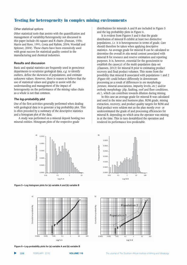
Testing for heterogeneity in complex mining environments
Other statistical tools that assists with the quantification andmanagement of variability/heterogeneity not discussed inthis paper include chi-square and R charts (Duncan, 1956;Harris and Ross, 1991; Costa and Rahim, 2004; Woodall andSpitzner, 2004). These charts have been extensively usedwith great success for statistical quality control in themanufacturing and chemical industries.
Basic and spatial statistics are frequently used in geosciencedepartments to scrutinize geological data, e.g. to identifyoutliers, define the skewness of populations, and estimateunknown values. However, there is reason to believe that theuse of statistical values and graphs to assist with theunderstanding and management of the impact ofheterogeneity on the performance of the mining value chainas a whole is not that common.
One of the first activities generally performed when dealingwith geological data is to generate a log-probability plot. Thisis often preceded by a summary of the descriptive statisticsand a histogram plot of the data.
A study was performed on a mineral deposit hosting twomineral entities. Histogram plots of the respective grade
distributions for minerals A and B are included in Figure 5and the log-probability plots in Figure 6.
It is evident from Figures 5 and 6 that the gradedistribution of mineral B exhibit at least two distinctivepopulations, i.e. it is heterogeneous in terms of grade. Careshould therefore be taken when applying descriptivestatistics. An average grade for mineral B can be calculated todetermine the overall in situ metal content associated withmineral B for resource and reserve estimation and reportingpurposes. It is, however, essential for the geoscientist toestablish the cause(s) of the multi-population data-set(Claassen, 2013) for mineral B prior to estimating productrecovery and final product volumes. This stems from thepossibility that mineral B associated with populations 1 and 2(Figure 6b) could behave differently in downstreamprocessing as a result of differences in ore morphology(texture, mineral associations, impurity levels, etc.) and/ororebody morphology (dip, faulting, roof and floor conditions,etc.), which can contribute towards dilution during mining.
In this case an average grade for mineral B was calculatedand used in the mine and business plan. ROM grade, miningextraction, recovery, and product quality targets for ROM andfinal product were seldom met as the plan mostly over- orunderestimated the grade of and processing efficiencies formineral B, depending on which area the operator was miningin at the time. This in turn destabilized the operation andrendered its performance less predictable.
�
184
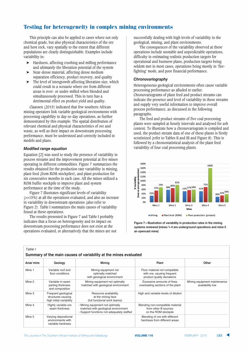
This principle can also be applied to cases where not onlychemical grade, but also physical characteristics of the oreand host rock, vary spatially to the extent that differentpopulations are clearly distinguishable. Examples includevariability in:
� Hardness, affecting crushing and milling performanceand ultimately the liberation potential of the system
� Near-dense material, affecting dense mediumseparation efficiency, product recovery, and quality
� The level of intergrowth affecting liberation size, whichcould result in a scenario where ore from differentareas is over- or under-milled when blended andsimultaneously processed. This in turn has adetrimental effect on product yield and quality.
Claassen (2015) indicated that few southern Africanmining operators link variable geological environments withprocessing capability in day-to-day operations, as furtherdemonstrated by this example. The spatial distribution ofrelevant chemical and physical characteristics of ore andwaste, as well as their impact on downstream processingperformance, must be understood and correctly included inmodels and plans.
Equation [2] was used to study the presence of variability inprocess streams and the improvement potential at five minesoperating in different commodities. Figure 7 summarizes theresults obtained for the production rate variability in mining,plant feed (from ROM stockpiles), and plant production forsix consecutive months in each case. All the mines utilized aROM buffer stockpile to improve plant and systemperformance at the time of the study.
Figure 7 illustrates significant levels of variability(>>15%) at all the operations evaluated, and also an increasein variability in downstream operations (also refer to Figure 2). Table I summarizes the main causes of variabilityfound at these operations.
The results presented in Figure 7 and Table I probablyindicates that a focus on heterogeneity and its impact ondownstream processing performance does not exist at theoperations evaluated, or alternatively that the mines are not
successfully dealing with high levels of variability in thegeological, mining, and plant environments.
The consequences of the variability observed at theseoperations include unstable and unpredictable operations,difficulty in estimating realistic production targets foroperational and business plans, production targets beingseldom met in most cases, operations being mostly in ’fire-fighting’ mode, and poor financial performance.
Heterogeneous geological environments often cause variableprocessing performance as alluded to earlier.Chronovariograms of plant feed and product streams canindicate the presence and level of variability in these streamsand supply very useful information to improve overallprocess performance, as discussed in the followingparagraphs.
The feed and product streams of five coal processingplants were sampled at hourly intervals and analysed for ashcontent. To illustrate how a chronovariogram is compiled andused, the product stream data of one of these plants is firstlyscrutinized (refer to Tables II and III and Figure 8). This isfollowed by a chronostatistical analysis of the plant feedvariability of four coal processing plants.
Testing for heterogeneity in complex mining environments
185 �
Table I
Summary of the main causes of variability at the mines evaluated
Area/ mine Geology Mining Plant Other
Mine 1 Variable roof and Mining equipment not Floor material not compatible floor conditions optimally matched with ore, causing frequent
with geological environment product quality deviations
Mine 2 Variable in-seam Mining equipment not optimally Excessive amounts of fines Mining equipment maintenance parting thickness matched with geological environment overloading sections of the plant availability lowand composition
Mine 3 Frequent geological Resource availability High and variable levels of dilution structures causing at the mining face
high initial variability (full functional work teams)
Mine 4 Highly variable ore - Mining equipment not optimally Blending non-compatible material seam thickness matched with geological environment from other B sources
- Support functions not adequately staffed on the ROM stockpile
Mine 5 Varying depositional Blending of ore with different environments with hardness from different areasvariable hardness

Testing for heterogeneity in complex mining environments
The chronovariogram illustrated in Figure 8 contains thefollowing key variability indicators:
� Sill—the total variance of the data-set was calculated at0.67% ash2
� Random variability or fundamental error [V0]—thesemivariance at time = 0 represents the sampling,preparation, and analytical error associated with thedata-set. In this case it is equal to 0.22% ash2 or0.22/0.67 = 32.8% of the total variance. V0 is obtainedby extrapolating the chronovariogram to time = 0.Generally a fundamental error associated withsampling, preparation, and analysis of 10% is assumedto be acceptable. The high value of nearly 33% impliesthat an effort should be made to investigate these stepsto establish what factors contribute towards this error
� Total process variability [V1]—the semivariance at thefirst time lag represents the sum of the randomvariability and the variability associated withprocessing. It is assumed that very little variability iscontributed towards total process variability by thematerial on the conveyor belt within one time-lag. Thisassumption should be validated for very complexenvironments. In this case V1 = 0.27% ash2 or0.27/0.67 = 40.3% of the total variance
� Process variability [V1- V0]— The difference betweenthe total process variability and the random variabilityis 0.06 ash2 or 0.06/0.67 = 9.0% of the total variance
� Cyclical variability [Vc ]—the cyclical variancerepresents the variance at the first or short range cycle,which amounts to Vc = 0.5 × amplitude = 0.5 × 0.14 =0.07% ash2 or 0.07/0.67 = 10.4% of the total variance.Mining operations often exhibit cyclical eventsincreasing variability in the system. These eventsinclude shift changes, resetting of equipment set-points, changes in equipment performance over time,etc. The short-range cycle visible in this example was aresult of changes made in the RD set-points of theplant’s dense medium cyclones. In this example, thelong-range cycle (9-12 hours) was linked to miningmoving from one mining area to another, i.e. a changein the plant feed quality
� Range (hours)— the range deduced from thechronovariogram in this instance is about 6.3 hours.The range indicates the optimal frequency of samplingrequired to adequately capture short-range variabilityin the stream. It can therefore be used to optimize plantsampling regimes based on the inherent variability inthe system (material being processed as well as thesystem/process variability) instead of just samplingbased on a time or mass setting.
The same approach was followed to study the variabilityin plant feed quality for four different coal processing plants.The data used was collected over a period of threeconsecutive months. The data and semivariances calculatedfrom the data are summarized in Tables IV and V,respectively. The values for the chronovariogram variabilityindicators were obtained from Figure 9 and are summarizedin Table VI.
�
186
Table II
Summary of hourly analytical data for product ash
Time Ash %
06h00–07h00 14.1
07h00–08h00 14.2
08h00–09h00 15.9
09h00–10h00 15.3
10h00–11h00 16.1
11h00–12h00 15.0
12h00–13h00 15.0
13h00–14h00 15.1
14h00–15h00 15.1
15h00–16h00 15.5
16h00–17h00 15.0
17h00–18h00 14.4
18h00–19h00 14.3
19h00–20h00 14.1
20h00–21h00 15.5
21h00–22h00 14.6
22h00–23h00 16.2
23h00–00h00 16.1
00h00–01h00 15.8
01h00-02h00 16.3
02h00–03h00 16.3
03h00–04h00 16.7
04h00–05h00 16.6
05h00–06h00 15.9
Variance 0.67
Table III
Semivariance calculated for product ash values
Time lag Semivariance (% ash2)
01 0.272 0.313 0.444 0.555 0.486 0.647 0.738 0.899 1.0010 0.8711 0.81

From Table VI the following findings should behighlighted:
� Sill—the total variance in plant feed ash is high forplants 1 and 4 at 45.6% ash2 and 31.7% ash2,respectively. For plant 1 the random variabilitycontributed about 20% and process variability about32% of the total sill value. Random variability (39.4%)and cyclical variability (34.7%) are the biggest
contributors to variability in the plant feed ash to plant 4
� Random variability [V0]—the relatively high randomvariability for plants 1, 3, and 4 is probabilityassociated with sampling, preparation, and analysiserrors as discussed earlier
Testing for heterogeneity in complex mining environments
187 �
Table IV
Summary of hourly analytical data collected over aperiod of three months for plant feed ash for fourcoal processing plants
Average % ash
Time Plant 1 Plant 2 Plant 3 Plant 4
06h00–07h00 35.6 25.6 33.3 18.8
07h00–08h00 35.8 31.3 39.5 23.6
08h00–09h00 38.1 33.9 32.1 23.6
09h00–10h00 46.1 28.6 28.2 24.4
10h00–11h00 35.8 30.9 35.6 19.7
11h00–12h00 31.5 31.2 31.8 23.5
12h00–13h00 26.5 29.3 27.3 28.2
13h00–14h00 26.6 28.8 30.5 27.2
14h00–15h00 26.5 28.7 31.5 26.8
15h00–16h00 49.1 28.9 28.9 21.3
16h00–17h00 30.9 30.5 32.6 25.0
17h00–18h00 40.1 31.8 34.5 26.9
18h00–19h00 36.1 32.0 31.6 31.8
19h00–20h00 30.9 31.3 31.6 35.4
20h00–21h00 26.2 30.9 37.1 39.3
21h00–22h00 36.0 32.4 32.2 25.0
22h00–23h00 36.7 31.8 29.7 25.0
23h00–00h00 28.8 29.8 28.9 19.4
00h00–01h00 22.1 31.6 43.1 20.1
01h00–02h00 31.1 28.8 28.2 25.9
02h00–03h00 42.2 31.1 33.4 32.8
03h00–04h00 31.1 31.0 39.2 27.0
04h00–05h00 26.9 17.8 37.3 38.8
05h00–06h00 26.6 26.4 33.1 27.4
Variance 45.6 10.1 15.9 31.7
Table V
Semivariance calculated for plant feed ash valuesfor four coal processing plants
Lag Semivariance (% ash2)
Plant 1 Plant 2 Plant 3 Plant 4
01 23.5 2.5 10.3 14.72 38.3 7.7 17.6 17.53 52.7 7.5 18.9 22.34 59.8 4.9 9.8 36.95 43.0 7.5 10.9 41.86 49.9 7.4 22.0 40.97 39.6 8.3 14.4 27.68 44.5 9.8 9.1 26.29 38.7 8.9 15.2 18.910 44.4 8.8 16.3 28.511 41.1 10.0 8.6 33.512 55.2 10.9 21.5 35.7
Note: variability expressed as a % of the population variance/sill value in bottom half of Table VI
Table VI
Statistical variance and errors calculated from chronovariograms plotted of plant feed ash variance for theprocessing plants under review
Variability indicator Plant 1 Plant 2 Plant 3 Plant 4
Population variance (sill) [% ash2] 45.6 10.1 15.9 31.7Random variability (V0) [% ash2] 9.0 0 2.5 12.5Total process variability (V1) [% ash2] 23.5 2.5 10.3 14.7Process variability (V1- V0) [% ash2] 14.5 2.5 7.8 2.2Cyclical variability [% ash2] 6.0 2.0 5.0 11.0Range (time lags) 2.5 11.8 1.8 3.7Random variability (V0) [%] 19.7 0 15.7 39.4Total process variability (V1) [%] 51.5 24.8 64.8 46.4Process variability (V1- V0) [%] 31.8 24.8 49.1 6.9Cyclical variability [%] 13.2 19.8 31.4 34.7

Testing for heterogeneity in complex mining environments
� Process variability [V1 - V0 ]—the feed ash variance forplants 1, 2, and 3 exhibits high upstream processvariability. In this case the variability was inducedduring mining operations, mainly as a result of highlyvariable geological environments and the inability toadjust to mining condition
� Cyclical variability [Vc ]—the feed to plants 3 and 4suffered from cyclical variability induced in upstreamoperations. It was established that the cyclic eventsrelated to mining frequently moving to different miningareas with different conditions and ore quality, i.e.about 5-hourly and 8-hourly cycles for plants 3 and 4,respectively
� Range (hours)—the results indicate that significantincreases in short-range variability from the first tosecond time lag (excluding plant 4) exist. Process andcyclical variability contributed the most towards theseincreases. In order to enable upstream functions totimeously manage the causes of variability, thefrequency of reporting analysis should probably beincreased. The total cycle time for sampling,preparation, analysis and reporting should be reducedto between 2 and 3 hours for the plants evaluated. Inall the cases the total cycle time for sampling,preparation, analysis and reporting was between 4 and5 hours.
Mining environments are heterogeneous or variable bynature. This variability directly impacts the use of descriptive,probabilistic, and inference statistics as well as an operation’sability to create a stable and predictable businessenvironment.
Descriptive, probabilistic, and inference statistics areapplied on the premise that a well-known homogeneouspopulation or representative sample of the population exist.For multi-population distributions, these statisticalcalculations should be approached with caution. A case inpoint is the inappropriate averaging or ‘mathematicalblending’ of grade values in a multi-grade deposit. Utilizingthese averages in mine and business plans can result inunrealistic plans that are seldom met and which in turn candestabilize mining operations. The study demonstrated that alog-probability plot is a good indicator of the existence ofmultiple populations in geological environments. It isimperative that geoscientists not only identify the presence ofmulti-population environments, but also establish the rootcause(s) of these populations, understand how they impactthe use of data in plans and models, and know how miningand plant operations should be set up to optimally processthese deposits. If variable geological environments areexploited without full consideration of the potential impact ondownstream processing performance, a ripple effect that runsdownstream through the processing chain may beexperienced.
In order to establish whether this effect can be detected inprocessing streams a modified range equation andchronovariography were applied to data obtained from fiveoperational mines and processing plants. The study reportedrelatively high production rate variability using the modifiedrange equation, varying between 26% and 160%, which is far
greater than the ’benchmark’ value of 15%. This was causedmainly by variable geological environments and miningoperators’ inability to effectively deal with the variability. Anincrease in production rate variability from the mining face tothe plant product stockpiles (variability increases furtherdown the mining value chain) of between about 15% andover 300% suggest that the root causes of variability havenot been identified and managed at the operations studied.
A ‘chronostatistical’ study conducted on plant feed andproduct streams at several coal processing operations alsofound high levels of variability in the systems. The resultsindicate that random variability (sampling, preparation, andanalysis), process variability (all processing activities), andcyclical variability (cyclical changes such as equipment set-point and shift changes) are the main contributing factorstowards relatively high overall variability found in the plantsstudied.
The study suggests that a focus on heterogeneity maysignificantly enhance overall mining performance as it createsan opportunity to understand inherent system variability andaddress instability and unpredictability in complex miningenvironments.
BARDOSSY, G. and FODOR, F. 2001. Traditional and new ways to handleuncertainty in geology. Natural Resource Research, vol. 10, no. 3. pp. 179–187.
CLAASSEN, J.O. 2013. Yield improvement at a mid-sized coal mine in theWitbank coalfields. Journal of the Southern African Institute of Miningand Metallurgy, vol. 113. pp. 761–768.
CLAASSEN, J.O. 2015. Application of systemic flow-based principles in mining.Journal of the Southern African Institute of Mining and Metallurgy, vol. 115, no. 8. pp. 747–754.
COSTA, A.F.B. and RAHIM, M.A. 2004. Monitoring process mean and variabilitywith one non-central chi-square chart. Journal of Applied Statistics, vol. 31, no. 10. pp. 1171–1183.
DUNCAN, A.J. 1956. The economic design of X charts used to maintain currentcontrol of a process. American Statistical Association Journal, June 1956.pp. 228–242.
FORRESTER, J.W. 1958. Industrial dynamics: a major breakthrough for decisionmakers. Harvard Business Review, vol. 38, July–August. pp. 37–66.
FOWLER, A. 1999. Feedback and feedforward as systemic frameworks foroperations control. International Journal of Operations and ProductionManagement, vol. 19, no. 2. pp. 182–204.
GY, P. 1983. Sampling of Particulate Materials, Theory and Practice.Developments in Geomathematics 4. Elsevier Scientific.
HARRIS, T.J. and ROSS, W.H. 1991. Statistical process control procedure forcorrelated observations. Canadian Journal of Chemical Engineering, vol. 69. pp. 48–57.
KRIGE, D.G. 1951. A statistical approach to some basic mine valuation problemsin the Witwatersrand. Journal of the Chemical, Metallurgical and MiningSociety of South Africa, December 1951. pp. 119–139.
MATHERON, G. 1960. Traité de géostatistique appliquée, tome i: Mémoires dubureau de recherches géologiques et minières, vol. 14. 333 pp.
MINNITT, R.C.A. and PITARD, F.F. 2008. Application of variography to the controlof species in material process streams: % Fe in an iron ore product.Journal of the Southern African Institute of Mining and Metallurgy, vol. 108. pp. 109–122.
PITARD, F.F. 1993. Pierre Gy’s Sampling Theory and Sampling Practise:Heterogeneity, Sampling Correctness and Statistical Process Control. 2ndedn. CRC Press, Boca Raton, Florida. 491 pp.
PITARD, F.F. 2006. Chronostatistics: a powerful, pragmatic, new science formetallurgists. Proceedings of Metallurgical Plant Design and OperatingStrategies, Perth, Australia, 18–19 September 2006. Australasian Instituteof Mining and Metallurgy, Melbourne. 22 pp.
TOWILL, D.R. 1996. Industrial dynamics modelling of supply chains.International Journal of Physical Distribution and Logistics Management,vol. 26, no. 2. pp. 23–42.
WIKNER, J., TOWILL, D.R., and NAIM, M.M. 1991. Smoothing supply chaindynamics. International Journal Production Economics, vol. 22, no. 3.pp. 231–248.
WOODALL, W.H. AND SPITZNER, D.J. 2004. Using control charts to monitor processand product quality profiles. Journal of Quality Technology, vol. 36, no. 3.pp. 309–320. �
�
188
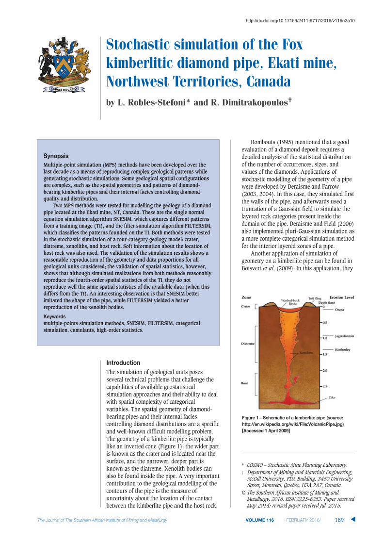
The simulation of geological units posesseveral technical problems that challenge thecapabilities of available geostatisticalsimulation approaches and their ability to dealwith spatial complexity of categoricalvariables. The spatial geometry of diamond-bearing pipes and their internal faciescontrolling diamond distributions are a specificand well-known difficult modelling problem.The geometry of a kimberlite pipe is typicallylike an inverted cone (Figure 1); the wider partis known as the crater and is located near thesurface, and the narrower, deeper part isknown as the diatreme. Xenolith bodies canalso be found inside the pipe. A very importantcontribution to the geological modelling of thecontours of the pipe is the measure ofuncertainty about the location of the contactbetween the kimberlite pipe and the host rock.
Rombouts (1995) mentioned that a goodevaluation of a diamond deposit requires adetailed analysis of the statistical distributionof the number of occurrences, sizes, andvalues of the diamonds. Applications ofstochastic modelling of the geometry of a pipewere developed by Deraisme and Farrow(2003, 2004). In this case, they simulated firstthe walls of the pipe, and afterwards used atruncation of a Gaussian field to simulate thelayered rock categories present inside thedomain of the pipe. Deraisme and Field (2006)also implemented pluri-Gaussian simulation asa more complete categorical simulation methodfor the interior layered zones of a pipe.
Another application of simulation ofgeometry on a kimberlite pipe can be found inBoisvert et al. (2009). In this application, they
Stochastic simulation of the Foxkimberlitic diamond pipe, Ekati mine,Northwest Territories, Canadaby L. Robles-Stefoni* and R. Dimitrakopoulos†
Multiple-point simulation (MPS) methods have been developed over thelast decade as a means of reproducing complex geological patterns whilegenerating stochastic simulations. Some geological spatial configurationsare complex, such as the spatial geometries and patterns of diamond-bearing kimberlite pipes and their internal facies controlling diamondquality and distribution.
Two MPS methods were tested for modelling the geology of a diamondpipe located at the Ekati mine, NT, Canada. These are the single normalequation simulation algorithm SNESIM, which captures different patternsfrom a training image (TI), and the filter simulation algorithm FILTERSIM,which classifies the patterns founded on the TI. Both methods were testedin the stochastic simulation of a four-category geology model: crater,diatreme, xenoliths, and host rock. Soft information about the location ofhost rock was also used. The validation of the simulation results shows areasonable reproduction of the geometry and data proportions for allgeological units considered; the validation of spatial statistics, however,shows that although simulated realizations from both methods reasonablyreproduce the fourth-order spatial statistics of the TI, they do notreproduce well the same spatial statistics of the available data (when thisdiffers from the TI). An interesting observation is that SNESIM betterimitated the shape of the pipe, while FILTERSIM yielded a betterreproduction of the xenolith bodies.
multiple-points simulation methods, SNESIM, FILTERSIM, categoricalsimulation, cumulants, high-order statistics.
* COSMO – Stochastic Mine Planning Laboratory.† Department of Mining and Materials Engineering,
McGill University, FDA Building, 3450 UniversityStreet, Montreal, Quebec, H3A 2A7, Canada.
© The Southern African Institute of Mining andMetallurgy, 2016. ISSN 2225-6253. Paper receivedMay 2014; revised paper received Jul. 2015.
189 �
http://dx.doi.org/10.17159/2411-9717/2016/v116n2a10

Stochastic simulation of the Fox kimberlitic diamond pipe, Ekati mine
�
190
built a stochastic simulation of the geometry of a kimberlitepipe conditioned to a piercing point’s data-set. Thesimulation was conducted on the cylindrical space bytransforming x-y-z coordinates to -r-z (rotation angle,radius, elevation) coordinates. A vertical trend was definedfor the radius, as it decreases towards the bottom of the pipe.However, this methodology assumes that the walls of thepipe are smooth and cylindrical, making it hard to use formore complex kimberlite models. A possible inconvenience isthat the transformation of the coordinates may lead to anorder problem when back-transforming the simulated values.The main drawback of the method is that the wrapping of therotation angle may not ensure continuity in the points beingsimulated at each level.
The reproduction of complex geological features presentin kimberlite pipes can be addressed with newer multiple-point (MP) methods. MP modelling techniques focus onreproducing the geological patterns and shapes of orebodies;for example, they focus on the reproduction of complexspatial arrangements, such as xenoliths in the diatreme partof a pipe. Other than the MP methods discussed next andapplied herein, related methods in the technical literatureinclude those of Daly (2004) and Kolbjørnsen et al. (2014),who worked on a multiple-point approach focused on Markovrandom fields. Tjelmeland and Eidsvik (2004) applied ametropolis algorithm for sampling multimodal distributions.Arpat and Caers (2007) and Honarkhah and Caers (2012)developed computer graphic methods to reproduce patterns inimages. Gloaguen and Dimitrakopoulos (2009) implementeda simulation algorithm based on the wavelet decompositionof geophysical data and analogues of the geological model;this method is able to reproduce nonstationarycharacteristics. This framework was extended to MPsimulations for both categorical and continuous variables byChatterjee et al. (2012) and Chatterjee and Dimitrakopoulos(2012). Mustapha and Dimitrakopoulos (2010) presentedhigh-order simulations based on conditional spatialcumulants.
Multiple-point methods are based on the use of trainingimages (TIs), which are interpretations or analogues of thepossible geological patterns that underlie the phenomenonstudied. The TIs usually have a regular spatial configuration,which facilitates the inference of spatial patterns and theirprobability of occurrence. Templates are used for scanningTIs that represent information about a particular geologicalmodel. A pattern is a possible configuration of valuesobtained by scanning the TI with the template. Single normalequation simulation (SNESIM) is a fast MP simulationalgorithm developed by Strebelle (2002) as an extension ofpast approaches (Guardiano and Srivastava, 1993). Whenusing SNESIM, the patterns are saved in a tree-like datastructure, together with their conditional proportions. Anapplication of this method to the modelling of a curvilineariron deposit can be found in Osterholt and Dimitrakopoulos(2007). The latter work reports a known limit of the MPmethods, i.e. their inability to always reproduce the two-pointspatial relations in the data available, although all statisticsof the TI are reproduced. MP methods are TI-driven asopposed to data-driven, and when there are differencesbetween the higher order relations in the data and the TI, theTI characteristics prevail.
Filter-based simulation or FILTERSIM (Zhang et al.,2006; Wu et al., 2008) is a MP simulation method thatassociates filter scores to patterns. This recent simulationapproach groups patterns into classes of patterns. Theclassification of patterns is made according to a small set ofscores per pattern. The score is obtained by applying filterfunctions to the values at the template nodes. The underlyingassumption is that similar patterns will have similar scores.During the pattern simulation, the selection of the class fromwhich the pattern will be retrieved is given by measures ofdistance and similarity.
In the present study, first, the SNESIM and simulationusing filters (FILTERSIM) are revisited. Then, the twomethods are used to stochastically simulate lithologycategories of the Fox diamond-bearing kimberlitic pipe,located on the Ekati property, Northwest Territories. Finally,the performance of the stochastic outputs from SNESIM andFILTERSIM outputs are compared and validated in terms ofthe high-order statistics reproduced.
Sequential simulation offers a class of stochastic simulationalgorithms (Ripley, 1987). In particular, sequentialsimulation is also part of the MP simulation algorithms usedhere. The basic concept consists of modelling and samplinglocal conditional distribution functions (cdfs) at each node ofa grid. The multivariate N-point cdf of a stationary randomfield can be written as a product of N univariate cdfs(Equation [1]),
[1]
The following description of a single normal equation followsthe one presented in Guardiano and Srivastava (1993).Consider the existence of an unsampled location x0, and anevent A0 at that location. At each data location there is a dataevent A ; a simple data event would be a single datumA :{Z(x ) = z }, and a complex data event would be thewhole data-set S(n):{Z(x ) = z , = 1,...,n}.
The conditional probability of the event A0 given the ndata events A = 1, = 1,...,n, is equal to the conditionalexpectation of the indicator random variable A0.
is the single indicator of the global data
event S(n) = 1 that occurs if, and only if, all elementary dataevents occur simultaneously, . Given thisrelationship, the system of normal equations can be reducedto a single one (Equation [2]):
[2]

Stochastic simulation of the Fox kimberlitic diamond pipe, Ekati mine
191 �
[3]
Equation [3] can be read as a Bayes relationship forconditional probabilities; the result of indicator kriging usinga single global data event is equivalent to the Bayespostulate. Equation [3] can be expressed in probability terms:
These probabilities can be obtained from real data-sets orTIs by scanning them. In particular, E{A0.S(n)} is thefrequency of occurrence of the joint event, and E{S(n)} is thefrequency of occurrence of the global data event.
SNESIM was proposed by Strebelle (2002) and itscomputational aspects were since revisited and improved(Strebelle and Cavelius, 2014). In the SNESIM algorithm a TIis scanned in order to infer the relative frequencyE{A0|S(n)=1}. Each pattern scanned on the TI is saved in abinary search tree together with its conditional probability.Each pattern is saved in the tree, and every pattern is a leafof the tree. The conditional probability of a particular patternis calculated by counting the frequency of appearance of thepattern in the TI. The root of the tree contains the simplestsearch templates, and moving towards the leaves, thetemplate size increases given that more possibleconfigurations are available. The tree is constructed from theTI occurrences, not from the total number of theoreticaloccurrences.
Afterwards, a simulated value at node x0 is obtained bydrawing a realization of A0 using Monte Carlo simulationmethods. The sequential simulation rule is implemented suchthat each simulated value is kept as a data event forsubsequent nodes. The global data event will grow by oneunit S(n+1); if N nodes are simulated the last node will havea data event of size (n + N – 1). Simplification suggestskeeping just the nearest conditioning data events, reducingthe number n and complexity of data events. The SNESIMalgorithm can be applied only to categorical variables. As anexample, when using five categories and a data event of 16nodes (K = 5 and n = 16), there are up to Kn = 1.5 x 10¹¹
joint realizations of the n data values. This should not be aproblem if there is consistency between the hard data and theTI, so the data event is easily found during the scanning ofthe training image.
SNESIM is reasonable in its computational aspects, as ituses less CPU time by scanning the TI once. The conditionalprobabilities and the patterns are saved in a data structure;this facilitates the search when performing the simulationwithout demanding excessive RAM. Computational aspects ofSNESIM have recently been revisited and further improved(Strebelle and Cavelius, 2014). One limitation is related to thescope of the studies that can be done using this method,given that it works only using categorical data. Anotherlimitation is that discontinuities or nonstationaritybehaviours in the TI will not be reflected in the simulationoutputs, unless enough conditioning data is available giventhat local information is lost when saving patterns in thesearch tree. Another drawback is that when finding the dataevent, the hard data locations are moved to the closest nodein the search template configuration; however, this induces ascreen effect and other close data values could be ignored.
1. Scan the training image with particular data template n ofn nodes. Store the patterns along with the cdfs in a searchtree. The cdf is calculated using the Bayes relationship.The total number of occurrences of the data event is(c(dn)), and the number of times this data event has acentral value belonging to class k is defined as (ck(dn))
2. Each node on the grid is visited once along a randompath. At each node u, obtain the conditioning data eventinside the data search neighbourhood W(u), which is asub-template of n. Then find this pattern on the tree, anddraw a realization of the central value by sampling fromthe conditional probability distribution function. Thecentral value is used as hard data for subsequentlysimulated nodes.
A two rock-phase training image and a squared template offour nodes are shown in Figure 1. The template is used toscan the TI; but only the inner nodes of the TI are used, toensure that all the nodes in the template are assigned aparticular rock value. The construction of the search treewould follow these steps:
1. Use the node located in the centre of the template tocount the frequency of coloured versus white nodeslocated on the inner part of the TI, in this case 4×4nodes giving a total of 16 (do not count the first andlast rows and columns). This gives a distribution of 9whites and 7 coloured. These frequencies are saved onthe head of the search tree
2. Use the template node in the centre and the one in theposition 1 to scan the TI. There are two possibilities;node 1 is either white or coloured. If the centre node iswhite, node 1 is white 4 times and coloured 5 times. Ifthe centre node is coloured, node number one is 6times white and 1 time coloured
3. Use three nodes in the template to scan the image:centre, node 1, and node 2. Now there are eight totalpossible combinations. For each possible combination,count how many times it appears in the TI. There isone pattern that does not exist on the TI, so instead ofeight we will have just seven possible patterns
4. Use the four nodes to scan the TI (centre, nodes 1, 2,and 3). The total number of possible combinations is16, but only 10 of the combinations are present in theTI
5. Use the five nodes to scan the TI (centre, nodes 1, 2,3, and 4). The total number of possible patterns is 32,but only 20 of the combinations appear in the TI.
The possible patterns will be the leaves of the search tree,and their frequency of appearance is registered on the tree.Figure 3 shows the final search tree for this small example. Itwill be noticed that simple configurations are in the root ofthe tree and the complex ones towards the leaves.
FILTERSIM is a multiple point simulation algorithm that wasintroduced by Zhang et al. (2006); it works with bothcategorical and continuous TIs (it was mostly developed forcontinuous TIs). The filter simulation consists of three mainsteps: filter score calculation, pattern classification, andpattern simulation.

Stochastic simulation of the Fox kimberlitic diamond pipe, Ekati mine
A set of mathematical functions called filters is applied tothe TI. The TIs are scanned using a template configuration.Each TI’s pattern has a set of filter scores. A template TJ ={x0;hj, j = 1...J} is a set of J points xj = x0 + hj j = 1... Jdescribed by the origin coordinates x0 and the offset distancehj. A filter is a set of weights associated with a template TJ.There are L filters functions for a template with J nodes {fl(hj)j = 1... J, l = 1...L}. A training pattern (pat) centred atlocation x of template TJ has a set of L scores associated thatare calculated using Equation [4].
[4]
In the case of K categories, the image is divided into K
binary indicators Ik(x) = { }k = 1... K.The filters are applied to each category, giving K x L scoresfor each pattern. A continuous TI is a particular case of acategorical TI with only one category.
There are three default filters (average, gradient, andcurvature) for each axis X – Y – Z. The template size is ni, foreach direction i; the filter node offset is i = –mi,...,+mi withmi = (ni – 1)/2; finally, the filters can be defined as:
There is a minimum of nine filters scores consideringthree default filters in 3D; three of which are shown in Figure 4 for the case of a diamond pipe TI. The main aspect ofFILTERSIM is the dimension reduction, where a pattern of Jnodes is reduced to only K x L scores.
From this set of scores, the patterns (pat) can beclassified and grouped into several pattern classes, calledprototype classes (prot), which assumes that similar patternswill have similar filter scores. A prototype (prot) is defined asthe pointwise average of all the patterns belonging to theprototype class, and it has the same number of nodes as thetemplate (Equation [5]).
[5]
The total number of replicates, c, corresponds to thenumber of patterns extracted from the TI that belong to thespecific prototype class.
The categorical prototype is a set of K proportion maps. Aproportion map gives the probability of a category prevailingat template location xi + hj (Equation [6]).
[6]
There are two options to classify and group patterns. Oneis to define arbitrary thresholds in the score space; this iscalled cross-partition. The other option is called K-meanpartition; and it applies clustering techniques in the scorespace.
Finally, sequential simulation is performed by drawingpatterns that honour the data-set. A conditioning data event(dev) is obtained from the neighbouring data using the sametemplate utilized to scan the TI. Hard data is moved into gridnodes for each simulated node x, then the set of scores iscalculated for that data event.
The closest pattern class (prot) is chosen by means of aminimum distance measure d(dev, prot) defined in Equation[7]. The final simulated object is pulled by random selectionfrom the set of patterns belonging to the selected patternclass. Afterwards, the pattern is pasted into the simulationgrid and is used as hard data for the next point beingsimulated. The simulation is made starting from a coarse gridand then continuing with finer grids, helping with thereproduction of large-scale and small-scale features.
[7]
The main advantages of this method are related to thespeed and computing performance; it is fast since it scans theTI once with a given template size. This algorithm is lessdemanding on RAM than SNESIM. In particular, the patterninformation is represented by a smaller set of filter scoresinstead of the larger template dimensions; this reductiongenerates an increase in the speed of the algorithm.
�
192
l if x belongs to kth category 0 otherwise

The counterpoint relates to the output simulations,because these will depend strongly on the size of the templatebeing used. Not only will the running times depend on thesize of the template; the quality of the simulation willdecrease when using large templates, by showing artifacts.On the other hand, a small template can miss some large-scale behaviours of the TI. In summary, a good qualitysimulation output will require a careful selection of thetemplate size. Also, the selection of the filter functions beingused is important; some filters may give redundantinformation about the TI, for example when the TI issymmetric. Another drawback of this method is therepositioning of the hard data information into grid nodeseach time a data event is obtained.
Repeat:1. Rescale to gth coarse grid2. Calculate scores using rescaled filters3. Divide (pat)s into (prot)classes4. Relocate hard conditioning data into grid Gg
5. For (each node u)a. Extract (dev) at ub. Find (prot) class using (dev, prot)c. Sample (prot) class to get (pat)d. Paste (pat) to realization
6. End for7. If g 1, take out hard conditioning data from Gg until all
multi-grids Gg have been simulated.
The Ekati property, located in the Northwest Territories inCanada, is one of the main diamond producers in the world.BHP Billiton has mined diamonds from Ekati since 1998. In2003, 150 kimberlite pipes had been found, and five of themwere being mined: Fox, Panda, Misery, Beartooth, and KoalaNorth. In June, 2002, BHP Billiton reported a total resource of113 Mt, with an average grade of 1.3 carats per ton (Dyck etal., 2004). Nowicki et al. (2003), reviewed the geology of thefive kimberlite pipes that are being mined on the Ekatiproperty.
The shape of the pipes is mainly like an inverted cone(Figure 1); the wider part of the pipe is known as the craterand is located near the surface and the narrower, lower partof the pipe is known as the diatreme. A very importantcontribution to the geological modelling of the contour of thepipe is the measure of uncertainty about the location of thecontact between the kimberlite pipe and the host rock, mainlybecause all the material inside the pipe is considered as oreand is sent to the processing plant. The mining operations atEkati are based on open pit designs where the usual miningbench is about 10 to 15 m high; moreover, the host rockquality is good enough to allow for a steep slope angle.
According to Nowicki et al. (2003), the Ekati pipes arecomposed mainly of volcaniclastic kimberlite material (VK),such as fine- to medium-grained crater sediments,resedimented volcaniclastic kimberlite (RVK) that isash/mud-rich to olivine-rich, and primary volcaniclastic orpyroclastic kimberlite (PVK).
Fox is the largest orebody, 550 by 630 m in area and 810 m in depth. Fox is situated within the biotite granodioriteof the Koala Batholith. In general, the wall rock contactfollows a circular shape and in detail it is irregular andstrongly controlled by faults; the wall rocks also includeseveral diabase dykes. Fox pipe has two different phases: anupper flared zone (100–150 m thick) that contains mainlymud-rich resedimented volcaniclastic kimberlite (mRVK) anda lower diatreme-shaped zone filled mainly with tuffisitickimberlite (TK). The contact between the crater and thediatreme zone is sharp. There are large granodiorite boulderswithin the TK phase, below the RVK phase, in the lower partof mRVK phase, and sporadically in the tuffisic kimberlite.
Drill-hole samples contain information about the samplelength, the number of diamonds found, and the bulk density.There are 8991 samples with lengths ranging from 0.01 to821.8 m; on average, samples are 5 m long. Compositing isnecessary to regularize the sample length. The maximumnumber of occurrences of stones is 44, and the average is 7stones. The average rock density is 2.1 t/m3.
As mining operations are based on open pit designs witha typical bench height of 10 m, this measure is chosen as thecomposite length. The composites were built respecting thelithological codes in order to have representative samples foreach rock category, which is the main objective of this casestudy. There are 3610 composites samples that have anaverage length of 9.9 m; the minimum length is 7 m and themaximum 10 m.
The association between the rock categories in the harddata-set (containing 44 rock categories) and the 3D solidsinterpreting geological zones (crater, diatreme, xenoliths, andhost rock) is not straightforward. The crossing of informationbetween lithological codes and rock solids leads to thefollowing classification:
� Granodiorites are associated with the host rock (code0)
� Resedimented kimberlites, olivine kimberlites, andsands are with the crater solid (code 1)
� Tuffisitic kimberlites and primary kimberlites areassociated with the diatreme solid (code 2)
� Breccias are associated with xenoliths (code 3).
Figure 5 shows a vertical section of the composited drill-hole samples classified into the previously mentioned rockcategories. Xenoliths are present inside the pipe’s crater andalso in the diatreme; these bodies are considered to be mainlywaste, so their geological modelling is interesting, since theirtonnage should be discounted from the total ore reserves.The composites samples, rock type proportions aresummarized in Table I.
Geologists provided three wireframe solids representingthe geological model of Fox kimberlite pipe (Figure 5). Thewireframes comprised the wide crater zone near the surface,the narrow diatreme zone at the bottom, and the xenolithbodies inside the pipe. The lentil-shaped circles around themiddle zone are xenolith orebodies. These solids are used asbase information for the construction of a TI. The TI is athree-dimensional grid with nodes 10×10×10 m apart; whichdimensions are 54×63×81. The origin is (X×Y×Z):(515060×7170200×-300). Each grid node can have one
Stochastic simulation of the Fox kimberlitic diamond pipe, Ekati mine
193 �

Stochastic simulation of the Fox kimberlitic diamond pipe, Ekati mine
value among the four phases; each phase has a numeric code:0 for host rock, 1 for crater, 2 for diatreme, and 3 forxenoliths.
It is interesting to observe how the proportions of thedifferent rock types change along the vertical direction in theTI. From top to bottom, the relative proportions werecalculated every 10 m; the graphic with the proportionsinformation is shown in Figure 6. The vertical axis shows therelative proportions of each of the four rock types, and thehorizontal axis the elevation. Level 1 is at the bottom of thepipe and level 81 near the surface. The proportion of nodesinside the pipe decreases with increasing depth as the pipe isnarrower at the bottom. There are four main xenolithclusters, mostly located between the vertical levels 40 and 65.In Figure 6, the area covered in colour by each rock type canbe used to calculate the total tonnage of that particular rocktype.
This TI does not meet the assumption of stationaritybecause the rock type proportions change considerably alongthe vertical axis. Also, the patterns do not repeat themselvesmultiple times. The lack of stationarity can be overcome byadding data in zones where hard data is scarce and there is astrong geological expectation for a given rock type. Forexample, granite (host rock) would be expected outside theboundaries of the pipe. The use of abundant soft data wasproposed to overcome the problem, because the conditioningstep should ensure the reproduction of trends and complexpatterns.
Soft data is added outside the pipe limits in a regular gridof 10×10×10 m. Thus, artificial hard information with rockcode 0 is added. The soft data generation process is doneusing an algorithm that grows a given 3D object. The numberof times the object grows is an arbitrary election based on thetolerance to geological uncertainty. In this example, the entirepipe (union of crater and diatreme solids) is used as the 3Dobject. At each iteration, the pipe grows 10 m along eachaxis; in particular, this means the closest nodes with code 0located at the pipe’s border become part of the pipe for thenext iteration. For this particular case study, the pipe hasbeen grown five times, giving 50 m to allow for geologicaluncertainty. The nodes outside the last ‘bigger’ pipe areselected as locations for soft information (host rock). Animage of the soft information added outside the boundariesof the pipe is shown in Figure 7.
The SNESIM algorithm was utilized to obtain a stochasticgeology model. The simulation grid size has 54×63×81 nodeslocated every 10×10×10 m. Soft data is included. Thealgorithm needs as input the global marginal distribution ofthe four categories; this was obtained by counting thenumber of nodes that belong to each category. From a total of275 562 nodes in the training image grid, 222 090 belong tohost rock, 23 434 to crater, 27 598 to diatreme, and 2440were xenoliths (proportions: 0.806 host rock, 0.085 crater,0.100 diatreme, and 0.009 xenoliths.).
�
194
Table I
Drill-holes and composites rock categoriesproportions
Type Code Number Frequency
Host Rock 0 906 25%
Crater 1 1035 29%
Diatreme 2 1461 40%
Xenoliths 3 208 6%
Total 3610 100%

The RAM requirement and running time are increased byaugmenting the number of nodes in the search template, butthis will lead to a better reproduction of the patterns existingin the TI. In this case, 80 nodes inside the search templateare selected. The election of the search template geometrywas isotropic with 50 m (five nodes) in the X, Y, and Zdirections.
The ‘minimum number of replicates’ parameter can bedescribed as the number of times a pattern similar to the dataevent is present in the TI; the minimum frequency of thatgiven pattern in the search tree. If this number of replicates ismet, a simulated pattern will be retrieved from the conditionalprobability distribution. In this case, the minimum number ofreplicates is unity; if there is just one replicate of the dataevent in the search tree this particular pattern will beretrieved with 100% probability. Three multiple grids arechosen to ensure the reproduction of large and small scalepattern continuity.
Ten realizations were generated in order to assess thegeological uncertainty. The running time was 5.78 minutes.Figure 8 shows a section view of four realizations obtained.SNESIM realizations respect the main geometricconfigurations; crater rocks are at the top, diatreme rocks areat the bottom, and xenoliths are inside the pipe; however, thexenoliths are choppy and scattered. The host rock wall is asnot as soft as in the TI. The SNESIM algorithm gives areasonable structural quality of its realizations; however, thequality of the simulations must be measured using high-order statistics.
Figure 9 shows the vertical level-by-level proportioncurves for each rock category and for every realization. Eachlevel has 54×63 blocks; there are 81 vertical levels. Eachblock is assigned to one of the four different rock codes.
There are ten realizations. Blue lines describe the number ofblocks with the host rock code, light blue lines those assignedto the crater, yellow lines the diatreme, and red lines thosebelonging to the xenoliths. Black lines show the proportionsof the rock types in the TI. In general, the realizations respectthe proportions of the three main rock categories (crater,diatreme, and host rock); however, the proportions ofxenolith rocks are underestimated. The realizations alsofollow the same level-by-level inflections of the proportioncurves. The TI and the realizations curves follow each otherclosely between the top level (around level 81) and thebottom level (around level 0), where there is more consistentconditioning information.
For the purpose of comparing between the TI and thestochastic realizations, cumulants of fourth order werecalculated (Dimitrakopoulos et al., 2009) When a fourth-order cumulant is calculated, three different directions areprovided. In this case, top-bottom, east-west, and north-south are chosen. The cumulant of fourth order is a 3D objectwith different cumulant values at each node. Each node inthe cumulant object can be specified by three lags ordistances to the origin, defining a search template. Thetraining image and the geological realizations are scannedusing this template, generating one cumulant value for onenode in the object. Cumulants can be calculated oncontinuous variables or indicator (0-1) variables(Dimitrakopoulos et al., 2010). Cumulants on the TI can becalculated if we label the crater, diatreme, and xenoliths ascode 1 (inside pipe) and the host rock as code 0 (outsidepipe). Another cumulant map can be obtained by labellingthe xenoliths as code 1 and the crater, diatreme, and hostrock as code 0 (outside xenoliths). Figure 10 shows thecumulant 3D objects calculated by scanning the TI multipletimes with multiple templates. The cumulant maps providestructural information on the general shape of the kimberlitepipe. Also, cumulants identify the main distances betweenxenolith bodies along the vertical level and their lentil-shapedstructure. The fourth-order cumulant maps on the compositedrill-hole samples were also calculated in Figure 11.Although the cumulant object is incomplete since thecomposite samples are not fully informed on space,nevertheless the main shape of the cumulant object isreproduced.
Stochastic simulation of the Fox kimberlitic diamond pipe, Ekati mine
195 �

Stochastic simulation of the Fox kimberlitic diamond pipe, Ekati mine
Figure 12 shows the cumulants of fourth order of onerealization obtained with SNESIM. The xenolith cumulantsshow a tail, which differs from the training image. Thecontinuity of the xenolith’s bodies in the simulated maps ispoor, and the cumulant map reflects this situation.
The categorical version of the FILTERSIM simulationalgorithm was used to obtain several conditional realizations,which produced a model of the geological uncertainty. Themost relevant parameters used are detailed as follows.
The template size strongly influences the running time ofthe algorithm. The running time does not follow a linearbehaviour when increasing the template size; this can beexplained as follows. FILTERSIM consist of three maincalculation parts – filter calculation for the training image;pattern classification, which may be dominant whenclustering into prototypes; and pattern simulation, which maybe dominant when finding the distance between the dataevent and different prototypes.
A larger template is conducive to finding fewer patternswhile scanning the TI; then, the minimum number ofexpected replicates should be reduced. With a larger templateit is harder to find a data event; then the algorithm startsdoing unconditional simulation, and the reproduction ofgeology becomes poorer. A smaller template produces a moreaccurate reproduction of the TI, more replicates for eachpattern, and then a better subdivision, but the running timeincreases. While decreasing the template does not mean
increasing the running time further; some smaller templatesreach simplicity in the patterns found, which decreases therunning time. The extreme case is a template size of a singlenode. In the case of a binary variable there will be two mainprototypes classes, 0 and 1; however, the quality of therealizations becomes useless as they show lack of continuityand, in the extreme case, a pure nugget effect.
Finally, the template size 5×5×7 was used for obtaining10 realizations in the four-phase case study. The patch sizeshould ideally be just one node, to be pasted into thesimulated grid, but in this case running time will increase,and this can also lead to lack of reproduction of small-scalepatterns. The patch size chosen is 3×3×5, which is smallenough to ensure the absence of artefacts and large enoughto have a reasonable running time.
The number of multiple grids used helps the reproductionof largescale and small-scale patterns; however, it makes therunning time longer. In this case study, two multiple gridswould be chosen. The minimum number of replicates is thepattern prototype splitting criteria, to split a parent class intochild classes. Only those parent patterns with more than 10occurrences are further split into child classes. In this casestudy, cross-partition is used, selecting four divisions as aparent splitting criteria at each filter score, and two assecondary splitting or child partitions. The data weights forhard, patch and other are 0.5, 0.3, and 0.2, respectively.
An image with an output of four realizations is shown inFigure 13. From a purely visual inspection, the realizationsseem to follow the main structural features of the pipe,generating xenolith bodies only inside the pipe boundariesand following closely the pipe’s cone shape. Somerealizations lose continuity in the crater phase near the topand in the diatreme phase at the bottom.
Figure 14 shows the vertical level-by-level proportioncurves for each rock category and for every FILTERSIMrealization. In general, the realizations respect theproportions of the three main rock categories (crater,diatreme, and host rock). The TI and the realizations curvesfollow each other closely between the top level (around level81) and the bottom level (around level 0), where there ismore consistent conditioning information. However, theproportions of xenolith rocks are underestimated; also, therealizations do not follow the TI xenolith curve tightly.Cumulants of fourth order of the FILTERSIM realizations areshown in Figure 15. The xenoliths cumulants appear tofollow the TI cumulants better than SNESIM.
�
196

The FILTERSIM running time is 16 807 529 ms (4.67 hours);which is large in comparison to the SNESIM simulation (346725 ms (0.1 hours). This can be explained mainly by the factthat the set of parameters chosen for FILTERSIM wasdemanding. The FILTERSIM algorithm requires less RAMthan SNESIM; in consequence, it takes a longer running time.The SNESIM algorithm is faster than FILTERSIM for the samestructural quality of its realizations. This gives a majoradvantage of SNESIM compared with FILTERSIM; the samegood simulation outcome can be obtained for less than 10%of the running time.
In order to compare the SNESIM and FILTERSIM realizationswith the TI, the global relative error was calculated usingEquation [8].
[8]
where N = 275562 is the total number of nodes in the TI. Thevalue of the cumulant of the stochastic realization j at node iis Vi
jis , and the value of the cumulant of the TI at node i is
ViTI. There is one global error for each stochastic realization.
As there are ten realizations, ten relative error values aregenerated, one for each cumulant map calculation (insidepipe and inside xenolith cases). The relative error betweenthe cumulant map calculated on the composites and the TIwas also calculated.
The summary of these calculations is shown in Table II.The total sum of the squared values of the TI N
Node i = 1 (ViTI)2
is 6085.59 for the inside/outside pipe cumulant map; and,18.04 for the inside/outside xenolith cumulant map. Relativeerrors in the reproduction of the cumulants of the wall of thepipe fluctuate around 1%; this means that the stochasticsimulation algorithms reproduce well the shape of the wall of
Stochastic simulation of the Fox kimberlitic diamond pipe, Ekati mine
197 �
Table II
Relative error of cumulant values
Global relative error
In/out pipe In/out xenoliths
SNESIM 0 0.528% SNESIM 0 25.02%
SNESIM 1 0.604% SNESIM 1 25.29%
SNESIM 2 0.980% SNESIM 2 22.31%
SNESIM 3 1.109% SNESIM 3 27.91%
SNESIM 4 0.526% SNESIM 4 23.88%
SNESIM 5 0.795% SNESIM 5 27.75%
SNESIM 6 0.991% SNESIM 6 22.89%
SNESIM 7 0.470% SNESIM 7 25.27%
SNESIM 8 0.416% SNESIM 8 25.61%
SNESIM 9 0.379% SNESIM 9 25.32%
Composites 26.85%
Sum (cumulant_TI2)
6085.59 18.23

Stochastic simulation of the Fox kimberlitic diamond pipe, Ekati mine
the pipe provided by the training image. Relative errorsfluctuate around 25% for the reproduction of the fourth-ordercumulants of the xenolith bodies. Relative errors are muchhigher in the reproduction of the cumulant values of thexenolith orebodies than in the reproduction of the cumulantsof the pipe wall. There is a difference of 26.85% between thecomposites and the TI. The composites’ cumulants followroughly the same shape of the cumulants calculated on theTI. The cumulant maps of the composite, as well as thetraining image and the realizations, were re-scaled. Giventhat the cumulants are used on an indicator variable, theyrepresent mainly geometric features of the map, so the re-scaling does not affect the error calculation because thecumulants are invariant to additional constants; moreover, ithelps to clarify the analysis of the errors. All of the cumulantmaps were re-scaled to a [0,1] interval, so the comparisonbetween the cumulant maps of the stochastic images, the TI,and the composites is more comprehensible.
With the purpose of validating FILTERSIM realizationsagainst the TI, the global relative error was calculated usingEquation [8]. There are ten realizations per simulationmethod, and ten relative error values are obtained for eachcumulant map calculation (inside pipe and inside xenolithcases). The summary of these calculations are shown inTable III. The relative errors in the reproduction of thecumulants of the wall of the pipe fluctuate around 2% forFILTERSIM. The FILTERSIM realizations’ errors for thexenolith maps fluctuate around 15%.
Relative errors are much higher in the reproduction of thecumulant values of the xenolith orebodies than in thereproduction of the cumulants of the pipe wall. FILTERSIMprovides better results than SNESIM for the reproduction ofthe continuity of the xenolith bodies because it simulatespatterns; however, the high relative errors reflect thedeficiency of both methods in reproducing the high-orderstatistics when simulating small or medium objectsdistributed in the geological domain.
The reproduction of the high-order statistics of thecomposites was analysed by calculating the global relativeerror with respect to the composite cumulant map. However,since the composite cumulant map is incomplete with respectto the other cumulant maps, only the set of nodes informedon both maps (composite cumulant map versus TI orrealizations cumulant maps) contribute to the errorcalculation. These nodes are called fully informed nodes.Equation [9] is used to obtain the global relative error.
[9]
where N = 22945 is the number of fully informed nodes. Theglobal relative errors are shown in Table IV. The total sum
NFully Informed Node i = 1 (Vi
Composites)2 is 6047.69 for theinside/outside pipe cumulant map. The inside/outsidexenolith cumulant global relative error was not calculatedsince the xenoliths composite cumulant map is poorlyinformed, and the relative errors do not provide usefulinformation. FILTERSIM errors fluctuate around 27.3% andSNESIM around 27.5%. FILTERSIM reproduces the
composites values slightly better. However, both stochasticmethods give a poor reproduction of the high-order statisticsof the composites.
The FILTERSIM method uses only a set of linear filters toclassify complex geological patterns; then, it may not possibleto reproduce nonlinear spatial correlations, i.e. high-orderspatial cumulants, of the TI from the simulated images.Furthermore, it is difficult to reproduce the high-order spatialnonlinear cumulants of complex geologic structures usingSNESIM, which is based on the calculation of only one linearhigh-order moment.
SNESIM and FILTERSIM were used for the stochasticsimulation of geology on the Fox kimberlite pipe. Fourcategories were used to simplify the geological model: crater,diatreme, xenoliths, and host rock. The training image (TI)
�
198
Table III
FILTERSIM relative error of cumulant values
FILTERSIM global relative error
In/out pipe In/out xenoliths
FILTERSIM 0 1.550% FILTERSIM 0 17.81%
FILTERSIM 1 2.101% FILTERSIM 1 13.11%
FILTERSIM 2 1.835% FILTERSIM 2 17.86%
FILTERSIM 3 1.604% FILTERSIM 3 14.07%
FILTERSIM 4 1.364% FILTERSIM 4 10.05%
FILTERSIM 5 3.634% FILTERSIM 5 10.83%
FILTERSIM 6 3.141% FILTERSIM 6 7.63%
FILTERSIM 7 1.393% FILTERSIM 7 12.46%
FILTERSIM 8 1.226% FILTERSIM 8 19.70%
FILTERSIM 9 2.938% FILTERSIM 9 13.96%
Composites 26.85%
Sum (cumulant_TI2)
6085.59 18.23
Table IV
SNESIM and FILTERSIM relative error with respectto composite cumulant values
FILTERSIM - SNESIM global relative error
In/out pipe
FILTERSIM 0 27.06% SNESIM 0 27.50%
FILTERSIM 1 26.44% SNESIM 1 27.74%
FILTERSIM 2 27.84% SNESIM 2 27.62%
FILTERSIM 3 27.24% SNESIM 3 27.00%
FILTERSIM 4 27.96% SNESIM 4 27.60%
FILTERSIM 5 28.60% SNESIM 5 28.09%
FILTERSIM 6 26.74% SNESIM 6 26.91%
FILTERSIM 7 27.17% SNESIM 7 28.19%
FILTERSIM 8 26.94% SNESIM 8 27.31%
FILTERSIM 9 27.88% SNESIM 9 27.66%
TI 27.02%
Sum (cumulant_composites2) 6047.693.42

provided by the geologist was not stationary. The generationof soft conditioning information outside the boundaries of thepipe (host rock code) was necessary to obtain a goodreproduction of the shape of the pipe. SNESIM simulation ismuch faster than FILTERSIM. Both methods reasonablyreproduce the main proportions of the main rock categories(crater, diatreme, and host rock); however, both methodsunderestimate the xenolith proportions. Fourth-ordercumulants were calculated using three main lag directions:top-bottom, east-west, and north-south. Cumulants werecalculated on the TI, the composites and the stochasticrealizations obtained from SNESIM and FILTERSIM methods.The binary variables chosen for the cumulant calculation aredivided into two different rock grouping configurations(inside/outside pipe and inside/outside xenoliths). Theinside/outside pipe cumulants show the shape of the pipe,and the inside/outside xenoliths show the vertical distancesbetween the lentil-shaped xenolith bodies. The global relativeerror was calculated between the cumulant maps of the TIand the stochastic realizations. As the errors of theinside/outside pipe are relatively small, it can be concludedthat both methods provide a good reproduction of thetraining pipe’s shape; larger errors are obtained whencomparing the inside/outside xenoliths cumulants, indicatingthat SNESIM and FILTERSIM algorithms perform worse in thereproduction of the xenolith bodies than in the reproductionof the walls of the pipe. SNESIM reproduced the pipe’s shapebetter than FILTERSIM; however, FILTERSIM reproduced thexenolith bodies better than SNESIM.
The assessment of the reproduction of high-order spatialstatistics (fourth-order spatial cumulants) by the simulatedrealizations from the two MPS methods shows that while therealizations tend to reproduce the high-order statistics of theTI, they do not reproduce those of the available data, whichin this case study are different to those of the TI. Othermethods that may improve this are currently beinginvestigated.
The work in this paper was funded from NSERC CDR Grant335696 and BHP Billiton, as well NSERC Discovery Grant239019 and McGill’s COSMO Lab. Thanks are in order to BHPBilliton Diamonds and, in particular, Darren Dyck, BarrosNicolau, and Peter Oshust for their support, collaboration,data from Ekati mine, and technical comments.
ARPAT, G.B. and CAERS, J. 2007. Conditional simulation with patterns.
Mathematical Geology, vol. 39, no. 2. pp.177–203.
CHATTERJEE, S., DIMITRAKOPOULOS, R., and MUSTAFA, H. 2012. Dimensional
reduction of pattern-based simulation using wavelet analysis.
Mathematical Geosciences, vol. 44. pp. 343–374.
CHATTERJEE, S. and DIMITRAKOPOULOS, R. 2012. Multi-scale stochastic simulation
with wavelet-based approach. Computers and Geosciences, vol. 45.
pp. 177–189.
DALY, C. 2004. High order models using entropy, Markov random fields and
sequential simulation. Geostatistics Banff 2004. Leuangthong, O. and
Deutsch, C. (eds). Springer, Dordrecht, vol. 2. pp. 215–224.
DIMITRAKOPOULOS, R., MUSTAPHA, H., and GLOAGUEN, E. 2010. High-order
statistics of spatial random fields: Exploring spatial cumulants for
modeling complex, non-Gaussian and non-linear phenomena.
Mathematical Geosciences, vol. 42, no. 1. 6 pp. 5–97.
DYCK, D., OSHURST, P., CARLSON, J., NOWICKI, T., and MULLINS, M. 2004. Effective
resource estimates for primary diamond deposits from the Ekati Diamond
MineTM, Canada. Lithos, vol. 76, no. 1–4. pp. 317–335.
GLOAGUEN, E. and DIMITRAKOPOULOS, R. 2009. Two-dimensional conditional
simulations based on the wavelet decomposition of training images.
Mathematical Geosciences, vol. 41, no. 6. pp. 679–701.
GUARDIANO, F.B. and SRIVASTAVA, R.M. 1993. Multivariate geostatistics: beyond
bivariate moments. Geostatistics Troia 1992. Proceedings of the FourthInternational Geostatistics Congress, vol. 1. Soares, A. (ed.). (Kluwer
Academic Publishers, Dordrecht, The Netherlands. pp. 133–144.
HONARKHAH, M. and CAERS, J. 2012. Direct pattern-based simulation of non-
stationary geostatistical models. Mathematical Geosciences, vol. 44, no. 6.
pp. 651–672.
KOLBJØRNSEN, O., STIEN, M., KJØNSBERG, H., FJELLVOLL, B., and ABRAHAMSEN, P.
2014. Using multiple grids in Markov mesh facies modeling.
Mathematical Geosciences, vol. 46, no. 2. pp. 205–225.
MUSTAPHA, H. and DIMITRAKOPOULOS, R. 2010. High-order stochastic simulations
for complex non-Gaussian and non-linear geological patterns.
Mathematical Geosciences, vol. 42, no. 5. pp. 455–473.
NOWICKI, T., CRAWFORD, B., DYCK, D., CARLSON, J., MCELROY, R., OSHUST, P., and
HELMSTAEDT H. 2003. The geology of kimberlite pipes of the Ekati
property, Northwest Territories, Canada. Lithos, vol. 76. pp. 1–27.
OSTERHOLT, V. and DIMITRAKOPOULOS, R. 2007. Simulation of orebody geology
with multiple-point geostatistics – application at Yandi channel iron ore
deposit, WA, and implications for resource uncertainty. Orebody Modellingand Strategic Mine Planning, 2nd edn. Dimitrakopoulos,
R. (ed.). Spectrum Series 14, Australasian Institute of Mining and
Metallurgy. pp. 51–58.
RIPLEY, B. 1987. Stochastic Simulation. Wiley, New York.
ROSENBLATT, M. 1985. Stationary Sequences and Random Fields. Birkhäuser,
Boston. 285 pp.
STREBELLE, S. 2002. Conditional simulation of complex geological structures
using multiplepoint statistics. Mathematical Geology, vol. 34. pp. 1–22.
STREBELLE, S. and ZHANG, T. 2005. Non-stationary multiple-point geostatistical
models. Geostatistics Banff 2004. Leuangthong, O. and Deutsch, C. (eds.).
Part 1. Springer, Dordrecht. pp. 235–244.
STREBELLE, S. and CAVELIUS, C. 2014, Solving speed and memory issues in
multiple-point statistics simulation program SNESIM. MathematicalGeosciences, vol. 46, no. 2. pp. 171–186
TJELMELAND, H. and EIDSVIK, J. 2004. On the use of local optimisations within
Metropolis-Hastings updates. Journal of the Royal Statistical Society,Series B, vol. 66. pp. 411–427.
WU, J., BOUCHER, A., and ZHANG, T. 2008. A SGeMS code for pattern simulation
of continuous and categorical variables: FILTERSIM. Computers andGeosciences, vol. 34, no. 12. pp.1863–1876.
ZHANG, T., SWITZER, P. and JOURNEL, A. 2006. Filter-based classification of
training image patterns for spatial simulation. Mathematical Geology,
vol. 38, no. 1. pp. 63–80.
Stochastic simulation of the Fox kimberlitic diamond pipe, Ekati mine
199 �

Stochastic simulation of the Fox kimberlitic diamond pipe, Ekati mine
The experimental calculation of cumulants is detailedaccording to Dimitrakopoulos et al. (2010). A template
Tn+1h1,h2,...,hn is defined as a set of n points separated from the
point x by distances h1,h2,...,hn. Every vector hi is defined by a lag distance hi, a direction vector di and a supportiveangle ai. An example of a four-point template is shown inFigure 16, which shows three vector distances{h1
North,h2East,h3
Vertical,}. The experimental calculation of thethird- and fourth-order cumulants are based on average summations in (10) and (11). In this case, Nh1,h2 and Nh1,h2,h3
are the number of elements of each template T3h1,h2 and
T4h1,h2,h3.
[10]
[11]
When a fourth-order cumulant is calculated, threedifferent directions are provided. In this case, top-bottom,east-west, and north-south are chosen. The cumulant offourth order is a 3D object with different cumulant values ateach node. Each node in the cumulant object can be specifiedby three lags or distances to the origin, defining a searchtemplate. The training image and the geological realizationsare scanned using this template, generating one cumulantvalue for one node in the object. �
�
200
SUBSCRIBEof the SAIMM Journal
TO 12 ISSUESJanuary to December 2016
ORR1 910.00LOCAL
US$515.90OVERSEAS
per annum per subscription
For more information please contact: Kelly Matthee The Journal Subscription DepartmentTel: 27-11-834-1273/7 • e-mail: [email protected] or [email protected]
Website: http://www.saimm.co.za
� Less 15% discount to agents only
� PRE-PAYMENT is required
� The Journal is printed monthly
� Surface mail postage included
� ISSN 2225-6253
� with cutting-edge research � new knowledge on old subjects � in-depth analysis

In view of environmental concerns and theshortage of good-quality coking coal, theCOREX process was designed as a newironmaking technology, attracting wideattention (Fang et al., 2005). In this process,lump coal and a small quantity of coke aredirectly charged into the melter-gasifier, wherea high-quality reducing gas is generated forthe reduction of the iron ore (Kumar et al.,2009). In contrast to the conventional blastfurnace (BF) process, non-coking lump coal isused as the reducing agent and as the energysource, and the iron charge consists of lumpore and/or pellets, which results in theelimination of the coke oven and sinteringplant as well as a decrease in investment(Kumar et al., 2009; Liu et al., 2012).
Although the COREX process has madegreat progress, in current production practicethe energy consumption greatly exceeds thatof the BF, and it requires a certain amount ofcoke to maintain permeability of the semi-cokebed (Wang et al., 2008). In addition, theprocess consumes a lot of good-quality lump
ore and lump coal. The pyrolysis of coal is thefirst step in most coal conversion processes,such as carbonization, gasification, andcombustion (Aboyade et al., 2013). Thereaction behaviour of lump coals in the COREXmelter-gasifier is crucial, as it determinesenergy utilization and gas composition, as wellas the metallurgical properties and particle sizeof the semi-coke produced (Prachethan et al.,2011; Zhang et al., 2014). In order to optimizethe process and improve its competitiveness,the pyrolysis kinetics of Datong coal used inBaosteel’s COREX C-3000 facility was studied.
Generally, the Coasts-Redfern method (Xuet al., 2010), ‘model-free’ method (Xu et al.,2010), and DAEM method (Tang et al., 2005)are used to investigate the kinetics of coalpyrolysis. In the Coasts-Redfern method,commonly used mechanism functions areinserted into the non-isothermal kineticequation to fit the experimental data one-by-one. The mechanism function with the largestcorrelation coefficient is selected as the best(Zhang et al., 2013). In this process, thereaction order is often replaced by the apparentreaction order to obtain the best fit (Zhang etal., 2014). However, the physical and chemicalmeanings of the reaction model are ignored. Inthe ‘model-free’ method (or DAEM method),the activation energies under differentconversion rates can be calculated. However,there is no way to calculate the kineticmechanism functions and the relatedparameters (Xu et al., 2010; Tang et al.,2005). Therefore, based on the previousresearch, a sectioning method was proposed tostudy the kinetics of coal pyrolysis. The kineticparameters at different heating rates were
Study of the pyrolysis kinetics ofDatong coal using a sectioning methodby R. Du*†, K. Wu*†, X. Yuan*†, D. Xu*†, and C. Chao*†
Lump coals are currently employed to replace part of coke in the COREXmelter-gasifier for ironmaking. In order to optimize the process, thepyrolysis kinetics of Datong coal used in the COREX process was studied.A sectioning method is proposed to overcome certain shortcomings oftraditional methods for studying the pyrolysis of coal. Based on thesectioning method and the characteristics of the coal pyrolysis process, thetemperature range was divided into three intervals. In the first, theadsorbed gas and water of crystallization were removed; in the second, thecoal was transformed into semi-coke; and finally, the semi-coke wasfurther coked. Three models of reaction were then established to study thedifferent stages of the pyrolysis process: an interfacial chemical reactionmodel, a random pore model, and internal diffusion with shrinkingvolume. The results showed that the experimental data fitted the modelswell, with all correlation coefficients (r2) exceeding 0.97. Finally, themechanisms of reaction and kinetic parameters for each temperature rangewere derived, which laid a necessary foundation for optimizing the usageof non-coking coal in the COREX process.
ironmaking, COREX process, kinetics, coal pyrolysis; sectioning method.
* State Key Laboratory of Advanced Metallurgy,University of Science and Technology Beijing,Beijing, China.
† School of Metallurgical and Ecological Engineering,University of Science and Technology Beijing,Beijing, China.
© The Southern African Institute of Mining andMetallurgy, 2016. ISSN 2225-6253. Paper receivedJan. 2015; revised paper received Sep. 2015.
201 �
http://dx.doi.org/10.17159/2411-9717/2016/v116n2a11
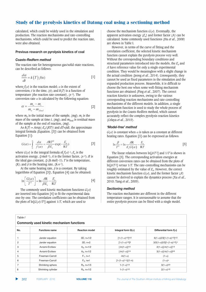
Study of the pyrolysis kinetics of Datong coal using a sectioning method
�
202
calculated, which could be widely used in the simulation andproduction. The reaction mechanisms and rate-controllingmechanisms, which could be used to predict the reaction rate,were also obtained.
The reaction rate for heterogeneous gas/solid-state reactions,can be described as follows:
[1]
where f( ) is the reaction model; is the extent ofconversion; t is the time, (s); and k(T) is a function oftemperature (the reaction rate constant), (s-1). Theconversion rate is calculated by the following equation:
[2]
where m0 is the initial mass of the sample, (mg); mt is themass of the sample at time t, (mg); and mfinal is residual massof the sample at the end of reaction, (mg).
As k(T) = Aexp(-Ea/(RT)) and dT= dt, the approximateintegral formula (Equation. [3]) can be obtained fromEquation [1]:
[3]
where G( ) is the integral formula of f( )-1; Ea is theactivation energy, (J·mol-1); A is the former factor, (s-1); R isthe ideal gas constant, (J·(K·mol)-1); T is the temperature,(K); and is the heating rate, (K·s-1).
At the same heating rate, is a constant. By takinglogarithms of Equation [3]), Equation [4] can be obtained:
[4]
The commonly used kinetic mechanism functions G( )are inserted into Equation [4] to fit the experimental dataone-by-one. The correlation coefficients can be obtained fromthe plots of ln[G( )/T2] against 1/T, which are used to
choose the mechanism function G( ). Eventually, theapparent activation energy (Ea) and former factor (A) can becalculated. Some commonly used functions (Hu et al., 2008)are shown in Table I.
However, in terms of the curve of fitting and thecorrelation coefficient, the selected kinetic mechanismfunction cannot explain the pyrolysis process very well.Without the corresponding boundary conditions andstructural parameters introduced into the models, the Ea andA have reference value for only a single experimentalcondition. They would be meaningless with a slight change inthe actual condition (Jeong et al., 2014). Consequently, theycannot be used as fixed parameters in the simulation and theexpanded production process. Meanwhile, it is difficult tochoose the best one when some well-fitting mechanismfunctions are obtained (Ping et al., 2007). The correctreaction kinetics is unknown, owing to the variouscorresponding reaction mechanisms and rate-controllingmechanisms of the different models. In addition, a singlemechanism function is used to study the whole process ofpyrolysis in the Coasts-Redfern method, which cannotaccurately reflect the complex pyrolysis reaction kinetics(Celaya et al., 2015).
G( ) is constant when is taken as a constant at differentheating rates. Equation [3] can be expressed as follows:
[5]
The linear relation between ln[ /T 2] and 1/T is shown inEquation [5]. The corresponding activation energies atdifferent conversion rates can be obtained from the plots ofln[ /T 2] versus 1/T. The rate-controlling mechanisms can beroughly estimated by the value of Ea. However, the correctkinetic mechanism function G( ), and the former factor (A)cannot be derived to explain the dynamics process (Xu et al.,2010; Tang et al., 2005).
The reaction mechanisms are different in the differenttemperature ranges. It is unreasonable to assume that theentire pyrolysis process can be fitted with a single model.
1 Jander equation 3D, n=1/2 [1-(1- )1/3]1/2 6(1- )2/3[1-(1-α)1/3]1/2
2 Jander equation 3D, n=2 [1-(1- )1/3]2 3/2(1- )2/3[1-(1-α)1/3]-1
3 Avrami-Erofeev A2, n=1/2 [-ln(1- )]1/2 2(1- )[-ln(1- )]1/2
4 Avrami-Erofeev A3, n=1/2 [-ln(1- )]1/3 3(1- )[-ln(1- )]2/3
5 Freeman-Carroll F1, n=1 -ln(1- ) (1- )
6 Freeman-Carroll F2, n≠1 [1-(1- )1-n]/(1-n) (1- )n
7 Shrinking sphere R3, n=1/3 1-(1- )1/3 3(1- )2/3
8 Shrinking cylinder R2, n=1/2 1-(1- )1/2 2(1- )1/2

Study of the pyrolysis kinetics of Datong coal using a sectioning method
203 �
Only the mathematical function for fitting can be derived, butthe rate-controlling mechanisms and corresponding kineticparameters cannot. Less is known about the entire pyrolysisprocess. Therefore, a sectioning method was proposed.
There are four steps in the sectioning method. First,according to the characteristics of the coal pyrolysis process,the temperature range is divided into different stages.Secondly, the appropriate kinetic models are established todescribe the different ranges of the pyrolysis process. Thefitting results are then acquired to verify the establishedmodels. Finally, the kinetic parameters of each stage arecalculated.
Compared to the traditional methods, the sectioningmethod emphasizes the physical and chemical meanings ofcoal pyrolysis kinetics, rather than a simple mathematicalfitting process. It was helpful in further studies of the coalresource. Furthermore, because the corresponding boundaryconditions and structural parameters were introduced to thekinetic models, the corresponding kinetic parameters of thepyrolysis process could be widely used in the simulation andexpanded production. Meanwhile, the reaction mechanismsand rate-controlling mechanisms were obtained, which couldbe used to predict the reaction rate.
Datong (DT) coal used in the Baosteel COREX C-3000 processwas used in the experimental work. The proximate, ultimate,and petrographic analyses are shown in Table II. According tothe classification standards for coal rank, DT coal belongs tothe bituminous class of coals.
A Netzsch STA 409 C thermogravimetric analyser wasused for the TGA experiments. Sample masses of between 10and 12 mg and particle size of 0.074–0.147 mm were used inthe experiments. The sample was held at room temperaturefor 40 minutes to remove the air, heated to 105°C at a rate of10°C·min-1, held at 105°C for 10 minutes to remove adsorbedwater, and then heated to 900°C at different heating rates (5,25, and 45°C·min-1). A gas flow of high-purity nitrogen (N2>99.999%) at 150 mL·min-1 was employed to protect thesample from oxidation. The change in the sample residualmass with respect to time and temperature change (TG data)was logged automatically by the computer.
The mass loss and derivative mass loss curves for thepyrolysis process at different heating rates are shown inFigures 1 and 2.
Regardless of the heating rate employed, the mainpyrolysis process of DT coal was roughly divided in twostages by Zhang (2013): the primary pyrolysis temperaturerange was from 300°C to 600°C; the secondary pyrolysisoccurred at temperature from 600°C to 800°C. In thispaper because changes of the kinetic mechanism are oftenaccompanied by radical changes in the mass loss rate, thetemperature range is divided into three parts at thetemperature where the regional variation of mass loss ratereaches the maximum. The ranges are shown in Table III.The temperature ranges are different at different heatingrates, the sectioning temperature points becoming higher asthe heating rate is increased.
In the low-temperature range, the heating rate has littleeffect on the mass loss rates, which remain at a low level.The adsorbed gas and crystalline water are removed.Meanwhile, the weak chemical bond of coal decomposes (Cui
59.30 7.57 26.21 6.92 69.71 4.72 0.99 10.62 1.33 32.6 1.7 7.0 58.7
Group maceral: Vit=vitrinite, Ex=exinite, Min=mineral, In=inertinite.

Study of the pyrolysis kinetics of Datong coal using a sectioning method
et al., 2007). The pyrolysis rate increases sharply at around386°C, which indicates the reaction mechanism and the rate-controlling mechanism are changing.
In the middle-temperature range, the rate of mass lossincreases rapidly, and the DTG curves remain at lower levels.This indicates that the pyrolysis rate is rapid. The reactionsoccurring are dominated mainly by depolymerization anddecomposition reactions, with evaporation of large amountsof coal gas, tar vapours, and water. As the temperatureincreases, the coal is transformed into semi-coke (Wu et al.,2014). Meanwhile, with increasing heating rate, the massloss of rate DT coal decreases, and the rate of pyrolysisshows a decline. At 464°C (25°C·min-1), the peak of massloss appears on the corresponding DTG curve, indicating thatthe pyrolysis reaction rate is at the maximum. With increasedheating rate, the maximum mass loss rate increases, and thetemperature corresponding to the peak shifts to the high-temperature region.
In the high-temperature range, the DTG curves graduallyshift upwards and approach zero with increasingtemperature, which indicates that the mass loss rate isdecreasing and the reaction is approaching completion. Thereactions taking place are dominated mainly bypolycondensation reactions with little tar and volatiles.Meanwhile, the semi-coke is further coked with an obviousvolume shrinkage (Fu et al., 2007). At the same temperaturewith the faster heating rate, the rate of pyrolysis of DT coalincreases at a slower rate. The effect of heating rate onpyrolysis rate decreases with increasing temperature (Cui etal., 2007).
According to the characteristics of each stage, the most likelykinetic mechanism functions were fitted to the thecorresponding range. Then, the models with the best fittingresults were chosen as the kinetic mechanism functions. Theresults indicated that the interfacial chemical reaction modelwith shrinking sphere, random pore model, and internaldiffusion model with shrinking volume were suitable fordescribing the different stages in the pyrolysis of DT coal.
The adsorbed gas and crystalline water are removed in thelow-temperature range. The gaseous products are easilyremoved from the solid product. Therefore, the interfacialchemical reaction model was used for the first phase. It wasassumed that the reaction particle A is a compact sphere; thereaction type is an interfacial chemical reaction; and thereaction equation is A (s) =aG (g) +bS (s) (Guo, 2006).
When the interfacial chemical reaction is the rate-controlling mechanism, the consumption rate of A is equal to
the interfacial chemical reaction rate, namely
The integral equation can be described as follows:
[6]
where 1=MA/ AR0; y1( )=1-(1- )1/3; the conversion rate is= (R3
0-r3)/R30; MA is the relative molecular mass of sample
A, 131×1.66×10-27 kg; A is the density of reactant A,1.28×106 g·m-3; r refers to the radius of reactant A, (m); andR0 refers to the initial radius of sample A, 1.11×10⁻⁴ m.
The function dT= dt and the equation krea1=A1exp(-Ea1/(RT)) are substituted into Equation [6] to yieldEquation [7].
[7]
where krea1 is the constant for the interface chemical reactionrate, (m·s-1); A1 is the former factor, (m·s-1); and Ea1 is thereaction activation energy, (J·mol-1).
According to the linear relationship of ln[y1( ) /T 2] and1/T in Equation [7], the slope and intercept of the curve canbe obtained in terms of the fitting results in the low-temperature range, and, Ea1, A1, and the function of krea1 andT can then be calculated.
Coal is transformed into semi-coke in the middle-temperaturerange. The reaction rate is related to the specific surface area,which is increased with a large number of pores forming. Therandom pore model was adopted to describe the process. Itwas assumed that the microporosity consisted of cylindricalholes with arbitrary radius, randomly distributed in the solidreactants; the pyrolysis reaction occurs mainly on thesurfaces of micropores; and (ignoring the effect of diffusion)the pyrolysis rate of coal is equal to the chemical reactionrate, which is proportional to the specific surface area (Gupta,et al., 2000; Wang, et al., 2006).
By introducing the pore structure parameters, the randompore model is applied to the gas-solid reaction process, whichhas a low conversion rate (approx. 0–0.6) and a maximum orgradually reducing reaction rate. The relationship for fittingcan be expressed as follows:
[8]
[9]
�
204
5 105–369 369–497 497–90025 105–386 386–524 524–90045 105–399 399–548 548–900

whereS0, isthe initial surface area, 7.46×10⁵ m2·m-3; L0 is the total lengthof the initial pore, 1.56×10¹¹ m·m-3; and 0 is the initial voidratio, 0=0.17 (dimensionless). S0 and 0 were measured bythe mercury intrusion method.
Similarly, Ea2, A2, and the function of krea2 and T can beobtained from the plots of ln[y2( )/T 2] against 1/T inEquation [9].
In the high-temperature range, the semi-coke is further cokedwith obvious volume shrinkage. With the high temperature,the chemical reaction rate is faster than the diffusion rate.The internal diffusion model with shrinking volume of theproduct was adopted (Zhang et al., 1988).
When gas internal diffusion is the rate-controlling step,the consumption rate of A is equal to the gas diffusion rate. Itmeets the relation D = a A, namely
The equation can be expressed as
follows:
[10]
where
V is the volume ratio of solid products and reactants, V=(R3X-
r3)/(R30-r3), V=0.733; ci and c0 are the gas concentration at
the internal and external surface the solid materialrespectively, ci= P /RT; c0=0 mol·m-3; D is the effectivediffusion coefficient, m2·s-1; D0 is frequency factor, m2·s-1; a isthe stoichiometric number of the gas products, which wastaken as 1; and Rx is the radius (m) of particle A attemperature Tm.
Similarly, Ea3 and D0 can be acquired from the plots ofln[y3( ) /T 2] vs. 1/T.
According to Table III, the experimental data for differenttemperature ranges at various heating rates were fitted byEquations [7], [9], and [10]), respectively. The results areshown in Figures 3, 4, 5, and Table IV. In the figures, thesymbols �, �, and � represent experimental data at thedifferent heating rates, and the lines the fitting results of themodels.
According to Figures 3, 4, 5, and Table IV, theexperimental data is a good fit, and all the correlationcoefficients (r2) exceed 0.97. Therefore, the interfacechemical reaction model, random pore model, and internaldiffusion model with the shrinking volume of product can beapplied to the low-, middle-, and high-temperature ranges ofthe pyrolysis process, respectively.
Based on the slopes and intercepts of the fitting curves andrelevant parameters, the kinetic parameters in threetemperature ranges at different heating rates were calculated.The results are listed in Tables V, VI, and VII.
Study of the pyrolysis kinetics of Datong coal using a sectioning method
205 �
5 0.9724 0.9917 0.993525 0.9716 0.9926 0.995945 0.9783 0.9935 0.9960
�

Study of the pyrolysis kinetics of Datong coal using a sectioning method
In Tables V, VI and VII, the activation energy at the samerate-controlling mechanism increases with the heating rate,but the magnitude of variation is less. The minimumactivation energy in the low-temperature range is from 14 to20 kJ·mol-1. Adsorbed gas and crystalline water are removedin this process, which needs less energy than the processes athigher temperatures. The maximum activation energy (93.7–116.3 kJ·mol-1) exists in the second temperature range. Themain reactions are macromolecule dissociation of coal andfurther decomposition of macromolecules in a split product,which need more energy. The activation energy with thelowest range, from 37 to 39 kJ·mol-1, corresponds to thehigh-temperature range. The semi-coke is coked further inthis temperature range. The observed activation energies,particularly in the low-and high-temperature ranges, arelower than that obtained by Zhang (2013), with a valuebetween 100 kJ/mol and 200 kJ/mol determined by theCoasts-Redfern method. The reason is that the experimentaldata should not have been calculated by G( ) for the entire
process, which leads to the error being introduced in theCoasts-Redfern method.
Furthermore, according to the variation in chemicalreaction rate constant and effective diffusion coefficient withtemperature (Tables V–VII), the kinetic parameters atdifferent temperatures were calculated. The results are shownin Tables VIII, IX, and X. By taking the logarithm of thekinetic parameters, the results are shown in Figure 6.
The reaction rate constant falls into the range 10-7–10-5 m·s-1. The magnitude of the effective diffusioncoefficient ranges from 10-10–10-8 m2·s-1. The value of thereaction rate constantly exceed the effective diffusioncoefficient by about 2–3 magnitudes, which conforms well tothe data measured by other researchers (Ferrara et al., 2014;Ishida, et al., 1968). In the non-isothermal thermodynamics,the reaction rate constant at a certain temperature is amomentary value, rather than a steady one. The heating ratehas an important influence on the Ea and A, hence the rateconstants are dependent on the heating rate. The chemical
�
206
5 105–369 1.47×10⁴ 2.19×10⁻⁴ lnkrea1 = -1.76×10³/T-8.4325 105–386 1.81×10⁴ 2.61×10⁻³ lnkrea1 = -2.17×10³/T-5.9545 105–399 2.00×10⁴ 4.49×10⁻³ lnkrea1 = -2.41×10³/T-5.41
5 369–497 9.37×10⁴ 6.17 lnkrea2 = -1.23×10⁴/T+1.8225 386–524 1.04×10⁵ 1.53×10² lnkrea2 = -1.25×10⁴/T+5.0345 399–548 1.16×10⁵ 3.39×10³ lnkrea2 = -1.40×10⁴/T+8.13
5 497–900 3.78×10⁴ 2.12×10⁻⁷ lnD = -4.54×10³/T-15.3725 524–900 3.80×10⁴ 4.31×10⁻⁷ lnD = -4.57×10³/T-14.6645 548–900 3.81×10⁴ 8.23×10⁻⁷ lnD = -4.58×10³/T-14.01
Table VIII
krea1 at different temperatures in the low-temperature range
Heating rate Temperature range Start krea1 at different temperatures (m·s-1) Final temperature
(°C·min-1) T (°C) temperature 200 (°C) 250 (°C) 300 (°C )
5 105–369 2.56×10⁻⁶ 5.70×10⁻⁶ 8.14×10⁻⁶ 1.10×10⁻⁵ 1.40×10⁻⁵
25 105–386 7.11×10⁻⁶ 2.26×10⁻⁵ 3.51×10⁻⁵ 5.04×10⁻⁵ 8.27×10⁻⁵
45 105–399 9.45×10⁻⁶ 3.50×10⁻⁵ 5.70×10⁻⁵ 8.52×10⁻⁵ 1.58×10⁻⁴

reaction rate constant or effective diffusion coefficientincrease with the heating rate at the same temperature, andalso increase with the temperature.
In order to overcome certain shortcomings of traditionalmethods in studying the pyrolysis process of coal, asectioning method was proposed in this paper.
1. According to the characteristics of Datong coalpyrolysis, the temperature range was divided intothree parts at the temperature where the regionalvariation of mass loss rate reached a maximum. Theadsorbed gas and crystalline water are removed in thelow-temperature range. With the evaporation of largeamounts of coal gas and tar, coal is transformed intosemi-coke in the second phase. In the third range, thesemi-coke is further coked
2. Different reaction mechanisms prevail in the threetemperature ranges. In terms of the characteristics ofDatong coal pyrolysis, the interfacial chemical reactionmodel, random pore model, and internal diffusion
model with shrinking volume of products were appliedto the different mechanisms
3. According to the divisions of temperature range andthe established models, the experimental dataobtained at different temperature ranges at variousheating rates were fitted. The results showed that theexperimental data was a good fit, and all thecorrelation coefficients (r2) exceeded 0.97. Theestablished models were therefore suitable fordescribing each range of the pyrolysis process
4. The corresponding kinetic parameters in each rangewere calculated at different heating rates. Theactivation energy increased with the heating rate atthe same rate-controlling mechanism. The chemicalreaction rate constant or effective diffusion coefficientincreased with the heating rate at the sametemperature, and also increased with temperature.
The authors are grateful for support from the NationalScience Foundation China (Grant No. 51274026, 51474022),
Study of the pyrolysis kinetics of Datong coal using a sectioning method
207 �
Table IX
krea2 at different temperatures in the middle-temperature range
Heating rate Temperature range Start krea2 at different temperatures (m·s-1) Final temperature
(°C·min-1) T (°C) temperature 400 (°C) 450 (°C) 500 (°C )
5 369–497 1.47×10⁻⁷ 3.29×10⁻⁷ 1.05×10⁻⁶ - 2.71×10⁻⁶
25 386–524 8.82×10⁻⁷ 1.31×10⁻⁶ 4.73×10⁻⁶ 1.45×10⁻⁵ 2.36×10⁻⁵
45 399–548 3.04×10⁻⁶ 3.14×10⁻⁶ 1.32×10⁻⁶ 4.63×10⁻⁵ 1.34×10⁻⁴
Table X
D at different temperatures in the high-temperature range
Heating rate Temperature range Start D at different temperatures (m2·s-1) Final temperature
(°C·min-1) T (°C) temperature 600 (°C) 700 (°C) 800 (°C )
5 497–900 5.80×10⁻¹⁰ 1.16×10⁻⁹ 1.98×10⁻⁹ 3.07x10⁻⁹ 4.40×10⁻⁹
25 524–900 1.40×10⁻⁹ 2.30×10⁻⁹ 3.94×10⁻⁹ 6.11×10⁻⁹ 8.78×10⁻⁹
45 548–900 3.11×10⁻⁹ 4.34×10⁻⁹ 7.43×10⁻⁹ 1.15×10⁻⁸ 1.66×10⁻⁸

Study of the pyrolysis kinetics of Datong coal using a sectioning method
the Independent Research Project of State Key Laboratory ofAdvanced Metallurgy and the National High-Tech (Grant No.41603003), University of Science and Technology Beijing(USTB), China.
ABOYADE, A.O., GÖRGENS, J.F., and CARRIER, M. 2013. Thermogravimetric study
of the pyrolysis characteristics and kinetics of coal blends with corn and
sugarcane residues. Fuel processing Technology, vol. 106. pp. 310–320.
CELAYA, A.M., LADE, A.T., and GOLDFARB, J.L. 2015. Co-combustion of brewer's
spent grains and Illinois No. 6 coal: Impact of blend ratio on pyrolysis and
oxidation behavior. Fuel Processing Technology, vol. 129. pp. 39–51.
CUI, Y.P., QIN, L.L., and DU, J. 2007. Products distribution and its influencing
factors for coal pyrolysis. Coal Chemical Industry, vol. 129, no. 2.
pp. 10–15.
FANG, J., WANG, XJ., and GUO, L. 2005. Energy consumption in smelting
reduction. Steel Research International, vol. 76, no. 10. pp. 705–708.
FERRARA, F., ORSINI, A., and PLAISANT, A. 2014. Pyrolysis of coal, biomass and
their blends: Performance assessment by thermogravimetric analysis.
Bioresource Technology, vol. 171. pp. 433–441.
FU, Z.X., GUO, Z.C., and YUAN, Z.F. 2007. Swelling and shrinkage behavior of
raw and processed coals during pyrolysis. Fuel, vol. 86. pp. 418–425.
GUO, H.J. 2006. Metallurgy Physical Chemistry. Metallurgical Industry Press,
Beijing.
GUPTA, J.S. and BHATIA, S.K. 2000. A modified discrete random pore model
allowing for different initial surface reactivity. Carbon, vol. 38, no. 1.
pp. 47–58.
HU, R.Z., GAO, S.L., and ZHAO, F.Q. 2008. Kinetics by Thermal Analysis.
Science Press, Beijing.
ISHIDA, M. and WEN, C.Y. 1968. Comparison of kinetic and diffusional models
for solid-gas reactions. AIChE Journal, vol. 14, no.2. pp. 311–317.
JEONG, H.M., SEO, M.W., and JEONG, S.M. 2014. Pyrolysis kinetics of coking coal
mixed with biomass under non-isothermal and isothermal conditions.
Bioresource Technology, vol. 155. pp. 442–445.
KUMAR, P.P., BARMAN, S.C., and REDDY, B.M. 2009. Raw materials for COREX
and their influence on furnace performance. Ironmaking and Steelmaking,
vol. 36, no. 2. pp. 87–90.
KUMAR, P.P., RAO, Y.S., CHIDAMBARAN, K., and RANJAN, M. 2009. Influence of coal
size on the performance of COREX process. Steel Research International,
vol. 80, no. 3. pp. 179–184.
LIU, Q.H., WU, K., and WANG, H.Y. 2012. Kinetic study of tar’s separation from
coals used in COREX. Journal of China Coal Society, vol. 37, no. 10.
pp. 1749–1752.
PING, C.J., ZHOU, J.H., and CHENG, J. 2007. Research on the pyrolysis kinetics of
blended coals. Proceedings of the CSEE, vol. 27, no. 17. pp. 6–10.
PRACHETHAN, K.P., RAJU, B.S.L., and RANJAN, M. 2011. Characteristics of coal
required for superior performance of COREX ironmaking. Ironmaking and
Steelmaking, vol. 38, no. 6. pp. 412–416.
TANG, W.J., WANG, C.X., and CHEN, D.H. 2005. Kinetic studies on the pyrolysis
of chitin and chitosan. Polymer Degradation and Stability, vol. 87.
pp. 389–394.
WANG, L., ZHANG, Z.T., and ZHANG, L. 2006. Study on modified random pore
model of catalytic coal char gasification. Journal of Xi’an Jiao Tong
University, vol. 40, no. 3. pp. 319–323.
WANG, N., XIE, X.M., and ZOU, Z.S. 2008. Analysis of material and energy
consumption of COREX C3000. Steel Research International, vol. 79,
no. 7. pp. 547–552.
WU, K., LIU, Q.H., and ZHAN, W.L. 2014. Research on tar precipitation kinetics
using phasewise analysis. Journal of Chemical Engineering of Chinese
Universities, vol. 28, no. 4. pp. 738–744.
XU, G.Y., PAUL, W. A., and NAOKO, E. 2010. Kinetic study on thermal
decomposition of flax fibers with model-free and Coats-Redfern model
fitting kinetic approaches. CIESC Journal, vol. 61, no. 9. pp. 2480–2487.
ZHANG, C.R., YANG, Y.G., and ZHANG, G. 1988. Kinetic model for solid state
reactions controlled by diffusion. Acta Physico-chimica Sinica, vol. 4,
no. 5. pp. 539–544.
ZHANG, J.L., WANG, G.W., and SHAO, J.G. 2014. A modified random pore model
for the kinetics of char gasification. BioResource, vol. 9, no. 2.
pp. 3497–3507.
ZHANG, S.F., ZHU, F., and BAI, C.G. 2014. High temperature pyrolysis behaviour
and kinetics of lump coal in COREX melter gasifier. Ironmaking and
Steelmaking, vol. 41, no. 3. pp. 219–228.
ZHANG, S.F., ZHU, F., and BAI, C.G. 2013. Thermal behavior and kinetics of the
pyrolysis of the coal used in the COREX process. Journal of Analytical and
Applied Pyrolysis, vol. 104. pp. 660–666. �
�
208

The prime objective of coal beneficiation is toremove physical impurities as effectively andeconomically as possible. The beneficiationprocess includes various operations on the as-mined coal to make it more suitable for end-use application without destroying the physicalidentity of the coal. There are several coalbeneficiation processes, but gravity-basedseparators remain the most efficient unitoperation for removing the undesirable ganguematerial from run-of-mine coal. Theseseparators exploit the difference in densitybetween coal particles and gangue particles toeffect a separation. The feed is introduced intoan aqueous suspension of ultrafine magnetitewith a particular density. The feed particleswith a relative density less than that of thesuspension (clean coal) float to the top surfaceof the suspension, whereas particles denserthan the suspension density (gangue material)sink to the bottom. When the difference indensity between the particle and the aqueoussuspension is large, the separation is easy, butwhen this difference is less the separationbecomes much more difficult since the settlingvelocity of the particles is very low. This lower
settling velocity increases the probability thatparticles that should report to floats report tosinks, and vice versa, hence increasing theamount of misplaced material. Therefore, thedegree of difficulty in beneficiating a typicalcoal at a particular specific gravity depends onthe amount of material occurring within ±0.1specific gravity range. This is known as ‘near-gravity’ material, also termed ‘near-dense’material, at that particular specific gravity ofseparation.
As coal is heterogeneous in nature, thedensity of a daughter coal particle depends onthe nature of the parent coal particle fromwhich it has been produced and the fracturepatterns involved during crushing, as shownin Figure 1. As the fracturing of particulatematerial is a random process and many factorscontribute to the fracturing of any singleparticle, the result is never exactly predictable.Particles of the same material and similar insize and shape show a wide variation inindividual fracture patterns. Therefore, when abigger heterogeneous particle of particulardensity is subjected to crushing a broadspectrum of particles of various sizes anddensities is produced. Similarly, when run-of-mine coal is crushed, a wide variety of smallerparticles are generated, which alters theamount of near-gravity material present in aparticular density class and accordinglychanges the degree of difficulty in washing.Therefore, it is imperative that the change inmass of the near-gravity material at aparticular specific gravity on crushing shouldbe determined accurately.
The difficulty in washing a particular coalcan be interpreted from the steepness of the‘characteristic curve’, which is derived fromthe sink-and-float data (Corriveau and
Effect of crushing on near-gravitymaterial distribution in different sizefractions of an Indian non-coking coalby S. Mohanta*, B. Sahoo*, I.D. Behera*, and S. Pradhan*
Run-of-mine coal contains particles of different sizes with differentspecific gravities, and when this coal is crushed, the amount of materialpresent in a particular density class changes. This alters the washabilitycharacteristics of the coal, which affects the quantity, quality, andseparation efficiency of the gravity-based coal washing process. Thedegree of difficulty in washing a typical coal at a particular specific gravitydepends mostly on the amount of material occurring within ±0.1 specificgravity range, which is known as ‘near-gravity material’ at that particularspecific gravity of separation. In this paper, two numerical indices, namely‘near-gravity material index’ and ‘index of washability’, are used toquantify the distribution of near-gravity material in different densityclasses and to evaluate the degree of difficulty involved in the washingprocess. The results of this preliminary investigation indicate the uniformdistribution of near-gravity material in all density classes for finer sizefractions, whereas for coarser size fractions more near-gravity material ispresent in the lower density classes, making the washing process moredifficult at a lower specific gravity of separation.
coal, coal cleaning, near-gravity material, index of washability.
* Department of Chemical Engineering, IndiraGandhi Institute of Technology, Sarang, India.
© The Southern African Institute of Mining andMetallurgy, 2016. ISSN 2225-6253. Paper receivedJul. 2015; revised paper received Oct. 2015.
209 �
http://dx.doi.org/10.17159/2411-9717/2016/v116n2a12

Effect of crushing on near-gravity material distribution in different size fractions
�
210
Schapiro, 1979; Osborne, 1988; Salama, 1989; Salama andMikhail, 1993). Also, several indices, coefficients, and factorssuch as the index of washability (Govindarajan and Rao,1994), washability number (Sarkar et al., 1977), andwashability index (Sarkar et al., 1962) have been proposedto quantify the amenability of a particular coal towardswashing, but none of them has gained wide acceptanceamong the coal preparation fraternity because each of theseparameters suffers from inherent limitations. In the presentwork, two simple parameters from the literature, namely‘near-gravity material index’ (NGMI) and ‘index ofwashability’ (IW), are reviewed and utilized to evaluate theeffect of crushing on the distribution of near-gravity materialin different density classes. The primary reason for selectingthe parameter IW for this study is that it varies between zeroand 100, thus facilitating quick interpretation, and providesan explicit equation and hence a precise evaluation of coalwashability characteristics is possible. Similarly, the NGMIvaries from zero to 1 for ‘easy to wash’ and ‘difficult to wash’coal respectively, thus also facilitating rapid interpretation.Moreover, the NGMI generates more useful information fromthe sink-and-float data for a typical coal and provides aneasier way to compare the washability characteristics ofdifferent coals quantitatively.
Govindarajan and Rao (1994) considered the float fraction ofthe sink-and-float analysis as the recovery of twoconstituents, namely non-ash (RN) and ash-forming (RA)materials, which can be calculated by the equations
100. X. (100–CA)RN = [1]100–HA
100. X. CARA = [2]HA
where X is the cumulative fractional weight of the feed coalfloated, and CA and HA are the ash percentages of the floatfraction and feed, respectively. Also, they observed that athree-constant cubic equation of the following form is a goodfit when the recovery curves for RN and RA are plotted againstcumulative fractional weight.
RN = aX + bX2 + cX3 [3]
RA = pX + qX2 + rX3 [4]
In order to demonstrate the calculation procedure, thesink-and-float analysis results of -150+25 mm size fractionof Ananta OCP coal is considered (Table I). The values for RN
and RA are calculated from Equations [1] and [2] and are tabulated in Table I. The recovery curves for non-ash and ash-forming materials (curve ADC and curve ABC inFigure 2) are drawn by plotting RN andRA values againstcumulative fractional weight. The values of the constants inEquations [3] and [4] are estimated by fitting theseequations to the non-ash and ash recovery curves and byusing the least squares method. In the present study acommercial software package named DataFit Version 8.0 isutilized to calculate the values for these constants. For float-and-sink data in Table I, the calculated values for a, b, c, p,q, and r are 128.17, –4.76, –22.93, 46.84, 8.99, and 43.26,respectively.
On considering the area bounded by these two curves forthe recoveries of non-ash and ash-forming material,Govindarajan and Rao (1994) proposed the index ofwashability (IW). The final form of the equation isrepresented as
{6a+ 4b +3c – 600} {6(a – p) + 4(b –q) +3(c – r)}IW = [5]
3600HA
This index of washability varies between zero and 100for the ‘unwashable’ and ‘easiest washable’ coal,respectively. For the data tabulated in Table I, the value of IWis found to be 15.259. The IW values for other size fractionsof coal are calculated following the same procedure.
Based on the same concept, Majumder and Barnwal(2004) proposed the ‘near-gravity material index’ (NGMI) fora better comparison between the coals. Curves ADC and ABCof Figure 2 represent the recovery curves for non-ash andash-forming materials, respectively. The amount of near-gravity material (NGM) at a particular specific gravity isdefined as the difference in cumulative fractional weightsfloated at ±0.1 specific gravity around that specific gravity.Using this definition with the data in Table I, the NGM at1.45 specific gravity may be calculated from the differencebetween the cumulative fractional weight floated at 1.55 andthe cumulative fractional weight floated at 1.35 (i.e. 0.737 –0.298 = 0.439). In terms of recovery of non-ash and ash-forming materials, the NGM distribution at 1.45 may be

Effect of crushing on near-gravity material distribution in different size fractions
211 �
represented geometrically by the area under KLMN in Figure 2. This area will be different at different specificgravities of separation for a particular coal. The near-gravitymaterial index can be calculated from the following equation:
[6]
As per the test programme, a coal sample of 4 t was collected(Indian Standard (IS):436, Part 1/Section 1) from AnantaOCP, and three representative samples prepared after coningand quartering the collected sample. Each representativesample was individually crushed to 150 mm, 100 mm, and50 mm in a laboratory-type roll crusher and the crushedproducts subjected to screen analysis.
Sink-and-float tests (IS: 13810) were conducted fordifferent size fractions. This test is conducted primarily todetermine how much coal of what quality can be produced ata given specific gravity with what separation complexity(Mitchell and Charmbury, 1963). Liquids in a range ofequally spaced specific gravity intervals from 1.4 to 2.0 areprepared, which include 1.4, 1.5, 1.6, 1.7, 1.8, 1.9, and 2.0.The liquids from density 1.4 to 1.6 are prepared fromsolutions of zinc chloride in water, and the rest by mixing
carbon tetrachloride and bromoform in different proportions.The separation tank is part-filled with the required liquid, therelative density of which is then checked using a suitablehydrometer. The relative density of the liquid is adjusted tothe correct reading and maintained at that value by frequentchecking to ensure that it remains within the range of ±0.002of the desired relative density for the duration of the test.
Each size fraction of coal obtained after screen analysis isintroduced into the tank containing the liquid of density 1.4and gently agitated. Care is taken not to overload the tank asthis is liable to interfere with the separation of entrained neargravity material. After allowing sufficient time for separation,the float material is removed and collected on a drainingplatform. The settled sink material is agitated to release anyentrained float material. Then, all the float materials arewashed in water, air-dried, and weighed for further analysis.The sink material is well drained and care is taken tomaintain the relative density of the succeeding liquid byintroducing only completely drained material from theprevious test. It is then introduced into the liquid of nexthigher relative density (density 1.5). The float material fromthis separation is also washed, air-dried, weighed, andprepared for further analysis. This procedure is repeated untilall the coal fractions have been tested at all relative densities.
The ash content of each sink-and-float fraction isdetermined as per IS: 1350. The ash content is determined byheating a weighed quantity of powdered coal (< 212 m) inan open crucible in presence of air to 500°C in 30 minutes,from 500 to 815°C for further 60 minutes, and maintained atthis temperature until a constant weight is achieved(approximately 60 minutes). The weight of residue is the ashcontent of the coal sample. A typical set of sink-and-floatdata for -150+25 mm size fraction is shown in Table I for therepresentative coal sample crushed to 150 mm.
On utilizing the sink-and-float data, the recovery curves forall the size fractions were drawn for each of the threerepresentative samples. Accordingly, the parameters for thecubic equation were calculated by fitting the equation to thedata points and adopting the least squares approach. Usingthese parameters and methodologies described earlier, theNGMI values were calculated and plotted as a function ofspecific gravity of separation as shown in Figure 3. It isinteresting to note that for all the three representativesamples, the pattern of the curves is similar. The NGMI ishigher at lower specific gravity of separation and decreases
Float at 1.4 1.36 29.8 17.6 29.8 17.6 37.57 15.141.4 to 1.5 1.45 25.5 29.8 55.3 23.2 64.96 37.081.5 to 1.6 1.55 18.4 37.2 73.7 26.7 82.64 56.841.6 to 1.7 1.65 8.8 47.1 82.5 28.9 89.76 68.801.7 to 1.8 1.75 5.2 52.9 87.7 30.3 93.51 76.741.8 to 1.9 1.85 4.2 57.6 91.9 31.6 96.23 83.731.9 to 2.0 1.95 3.6 63.1 95.5 32.7 98.26 90.28Sink at 2.0 2.22 4.5 74.8 100.0 34.6 100.00 100.00

Effect of crushing on near-gravity material distribution in different size fractions
with increasing specific gravity of separation. At lowerspecific gravity of separation the NGMI is highest for thecoarser size fraction, whereas at higher specific gravity ofseparation it is lowest. This indicates that the coarser sizefractions are more amenable towards washing at a higherspecific gravity of separation and the finer size fractions aremore amenable at a lower specific gravity of separation. Also,from Figure 3 it can be observed that the slope of the curvefor the finer size fraction is less than that for the coarser sizefraction. This indicates that the near-gravity material isdistributed more-or-less uniformly in all the density classesfor the finer size fractions. Therefore, the degree of difficultyinvolve in the separation process is almost same for finer sizefractions, bur for coarser size fractions the difficulty is greaterat lower specific gravity of separation due to the presence ofmore near-gravity material.
In order to clearly visualize the effect of crushing onnear-gravity material distribution in different density classes,the NGMI was plotted against specific gravity, as shown inFigure 4 for the coarsest and finest size fractions when the
three representative coal samples are crushed to 150 mm,100 mm, and 50 mm. It can be seen that the near-gravitymaterial is distributed more uniformly in all the densityclasses for both the size fractions when the coal is crushed to50 mm. Therefore, the slopes of the curves for the coalcrushed to 50 mm are less than the slopes of the curves forthe coal crushed to 100 mm or 150 mm. When the coal iscrushed to 50 mm, more finer particles are generated withvarious densities and these are equally distributed among allthe density classes; whereas when the coal is crushed to 150mm or 100 mm fewer finer particles are generated and mostof the particles are larger. As a result they are not equallydistributed in all the density classes.
The IW values for different size fractions of the coal werecalculated for the three representative coal samples crushedto 150 mm, 100 mm, and 50 mm and are shown in Table II.The IW values decrease with decreasing particle size for allthree samples, which indicates the uniform distribution of thenear-gravity material in all the density classes for smallersize fractions. A comparison between the coal crushed to 150mm and coal crushed to 50 mm shows that the near-gravitymaterial is distributed more uniformly between the densityclasses in the coal crushed to 50 mm.
The preliminary results of this investigation indicate thatfiner crushing results in the uniform distribution of the near-gravity material in all the density classes. This is probablybecause crushing generates a greater number of particleswith different specific gravities. Therefore, the difficulty
�
212
+25 15.259 12.064 17.354-25+13 26.556 25.811 22.783-13+6 30.653 32.223 25.786-6+3 40.813 38.115 33.490-3+0.5 42.393 42.603 38.138

involved in beneficiating finely crushed coal remains almostthe same for all specific gravities of separation. With coarsercrushing, more near-gravity material is present in the lowerdensity class than the higher density classes. Beneficiationtherefore becomes more difficult at a lower specific gravity ofseparation. However, this is a case-specific situation and itdepends on the nature of the mineral distribution in the run-of-mine coal.
The authors express their sincere thanks to The Institution ofEngineers (India) for funding the project (Project I.D.UG2014012). Sincere gratitude is also extended to the coalcompanies that provided the samples for this investigation.Finally, the authors express their thanks to all colleagueswho directly or indirectly contributed to the successfulcompletion of this study.
CORRIVEAU, M.P. and SCHAPIRO, N. 1979. Projecting data from samples. CoalPreparation. 4th edn. Leonard, J.W. (ed.). American Institute of Mining,Metallurgical, and Petroleum Engineers Inc., New York. Ch. 4, pp. 4–27.
GOVINDARAJAN, B. and RAO, T.C. 1994. Indexing the washability characteristicsof coal. International Journal of Mineral Processing, vol. 42. pp. 285–293.
INDIAN STANDARD. IS: 1350, (Part I): 1984. Methods of Test for Coal and Coke.(Reaffirmed 2001).
INDIAN STANDARD. IS: 436, (Part I/Sec 1): 1964. Methods of Sampling of Coaland Coke. (Revised 1981).
INDIAN STANDARD. IS: 13810: 1993. Code of Practice for Sink-and-float Analysisof Coal.
MAJUMDER, A.K. and BARNWAL, J.P. 2004. Development of a new coalwashability index. Minerals Engineering, vol. 17. pp. 93–96.
MITCHELL, D.R. and CHARMBURY, H.B. 1963. Cleaning and Preparation. Chemistryof Coal Utilization. Supplementary Volume. Lowry, H.H. (ed.). Wiley, NewYork. pp. 312–319.
OSBORNE, D.G. 1988. Coal Preparation Technology, Vol. I. Graham and Trotman,London. pp. 179–188.
SALAMA, A.I.A. 1989. Theoretical aspects of parallel coal processing circuits.International Journal of Mineral Processing, vol. 27. pp. 171–188.
SALAMA, A.I.A. and MIKHAIL, M.W. 1993. Balancing of raw washability datautilizing the least squares approach. Coal Preparation, vol. 13. pp. 85–96.
SARKAR, G.G., BOSE, R.N., MITRA, S.K., and LAHIRI, A. 1962. An index for thecomparison and correlation of washability characteristics of coal. IV CoalPreparation Congress, Harrogate. Paper E4.
SARKAR, G G., DAS, H.P., and GHOSE, A. 1977. Sedimentation patterns: do theyoffer clues to coal quality? World Coal. pp. 10–13. �
Effect of crushing on near-gravity material distribution in different size fractions
213 �
The Southern African Institute of Mining and Metallurgy and theMining Resilience Research Institute at the University of Pretoria
presents the
Resilience in the Mining IndustryConference 2016
African Mining Resilience - Strategic repositioning
For further information contact:Conference Co-ordinator, Camielah JardineSAIMM, P O Box 61127, Marshalltown 2107
Tel: (011) 834-1273/7Fax: (011) 833-8156 or (011) 838-5923
E-mail: [email protected] Website: http://www.saimm.co.za
13–14 July 2016: Conference, University of Pretoria

�
x
201617–18 May 2016 — The SAMREC/SAMVALCompanion Volume ConferenceJohannesburgContact: Raymond van der BergTel: +27 11 834-1273/7Fax: +27 11 838-5923/833-8156E-mail: [email protected]: http://www.saimm.co.za
18–19 May 2016 — Aachen International MiningSymposia (AIMS 2016) First InternationalConference Mining in EuropeAachen, GermanyContact: Conference Organisation of AIMSTel: +49-(0)241-80 95673Fax: +49-(0)241-80 92272E-mail: [email protected]: http://www.aims.rwth-aachen.de
21–28 May 2016 — ALTA 2016Perth, Western AustraliaContact: Allison TaylorTel: +61 (0) 411 692 442E-mail: [email protected]: http://www.altamet.com.au
9–10 June 2016 — New technology and innovationin the Minerals Industry ColloquiumMintek, RandburgContact: Camielah JardineTel: +27 11 834-1273/7Fax: +27 11 838-5923/833-8156 E-mail: [email protected]: http://www.saimm.co.za
27–28 June 2016 — The 2nd School on ManganeseFerroalloy ProductionJohannesburgContact: Raymond van der BergTel: +27 11 834-1273/7Fax: +27 11 838-5923/833-8156E-mail: [email protected]: http://www.saimm.co.za
13–14 July 2016 — Resilience in the MiningIndustry Conference 2016University of PretoriaContact: Camielah JardineTel: +27 11 834-1273/7Fax: +27 11 838-5923/833-8156 E-mail: [email protected]: http://www.saimm.co.za
25–26 July 2016 —Production of Clean SteelMintek, RandburgContact: Raymond van der BergTel: +27 11 834-1273/7Fax: +27 11 838-5923/833-8156E-mail: [email protected]: http://www.saimm.co.za
1–3 August 2016 — HydrometallurgyConference 2016‘Sustainability and the Environment’in collaboration with MinProc and the Western Cape BranchBelmont Mount Nelson Hotel, Cape TownContact: Raymond van der BergTel: +27 11 834-1273/7Fax: +27 11 838-5923/833-8156E-mail: [email protected]: http://www.saimm.co.za
16–18 August 2016 — The Tenth InternationalHeavy Minerals Conference ‘Expanding thehorizon’Sun City, South AfricaContact: Camielah JardineTel: +27 11 834-1273/7Fax: +27 11 838-5923/833-8156 E-mail: [email protected]: http://www.saimm.co.za
31 August–2 September 2016 — MINESafeSustaining Zero Harm ConferenceEmperors Palace, Hotel Casino Convention ResortContact: Raymond van der Berg
INTERNATIONAL ACTIVITIES

�xi
Tel: +27 11 834-1273/7Fax: +27 11 838-5923/833-8156E-mail: [email protected]: http://www.saimm.co.za
12–13 September 2016 — Mining for the Future2016 ‘The Future for Mining starts Now’Electra Mining, Nasrec, JohanannesburgContact: Camielah JardineTel: +27 11 834-1273/7Fax: +27 11 838-5923/833-8156 E-mail: [email protected]: http://www.saimm.co.za
12–14 September 2016 — 8th InternationalSymposium on Ground Support in Mining andUnderground ConstructionKulturens Hus – Conference & Congress, Luleå,SwedenContact: Erling NordlundTel: +46-920493535Fax: +46-920491935E-mail: [email protected]: http://groundsupport2016.com
19–21 October 2016 — AMI Ferrous and BaseMetals Development Network Conference 2016Southern Sun Elangeni Maharani, KwaZulu-Natal,South AfricaContact: Raymond van der BergTel: +27 11 834-1273/7Fax: +27 11 838-5923/833-8156E-mail: [email protected]: http://www.saimm.co.za
2017
25–28 June 2017 — Emc 2017: EuropeanMetallurgical ConferenceLeipzig, GermanyContact: Paul-Ernst-StraßeTel: +49 5323 9379-0Fax: +49 5323 9379-37E-mail: [email protected]: http://emc.gdmb.de
27–29 June 2017 —4th Mineral Project ValuationMine Design Lab, Chamber of Mines Building, TheUniversity of the Witwatersrand, JohannesburgContact: Raymond van der BergTel: +27 11 834-1273/7Fax: +27 11 838-5923/833-8156E-mail: [email protected]: http://www.saimm.co.za
2–7 October 2017 —AfriRock 2017: ISRMInternational Symposium ‘Rock Mechanics forAfrica’Cape Town Convention Centre, Cape TownContact: Raymond van der BergTel: +27 11 834-1273/7Fax: +27 11 838-5923/833-8156E-mail: [email protected]: http://www.saimm.co.za
INTERNATIONAL ACTIVITIES (continued)

�
xii
Company AffiliatesThe following organizations have been admitted to the Institute as Company Affiliates
3 M South Africa
AECOM SA (Pty) Ltd
AEL Mining Services Limited
Air Liquide (PTY) Ltd
AMEC Mining and Metals
AMIRA International Africa (Pty) Ltd
ANDRITZ Delkor(Pty) Ltd
Anglo Operations Ltd
Anglo Platinum Management Services (Pty) Ltd
Anglogold Ashanti Ltd
Atlas Copco Holdings South Africa (Pty) Limited
Aurecon South Africa (Pty) Ltd
Aveng Moolmans (Pty) Ltd
Axis House (Pty) Ltd
Bafokeng Rasimone Platinum Mine
Barloworld Equipment -Mining
BASF Holdings SA (Pty) Ltd
Bateman Minerals and Metals (Pty) Ltd
BCL Limited
Becker Mining (Pty) Ltd
BedRock Mining Support (Pty) Ltd
Bell Equipment Company (Pty) Ltd
Blue Cube Systems (Pty) Ltd
Bluhm Burton Engineering (Pty) Ltd
Blyvooruitzicht Gold Mining Company Ltd
BSC Resources
CAE Mining (Pty) Limited
Caledonia Mining Corporation
CDM Group
CGG Services SA
Chamber of Mines
Concor Mining
Concor Technicrete
Council for Geoscience Library
CSIR-Natural Resources and theEnvironment
Department of Water Affairs and Forestry
Digby Wells and Associates
Downer EDI Mining
DRA Mineral Projects (Pty) Ltd
DTP Mining
Duraset
Elbroc Mining Products (Pty) Ltd
Engineering and Project Company Ltd
eThekwini Municipality
Exxaro Coal (Pty) Ltd
Exxaro Resources Limited
Fasken Martineau
FLSmidth Minerals (Pty) Ltd
Fluor Daniel SA (Pty) Ltd
Franki Africa (Pty) Ltd Johannesburg
Fraser Alexander Group
Geobrugg Southern Africa
Glencore
Goba (Pty) Ltd
Hall Core Drilling (Pty) Ltd
Hatch (Pty) Ltd
Herrenknecht AG
HPE Hydro Power Equipment (Pty) Ltd
Impala Platinum Limited
IMS Engineering (Pty) Ltd
Ivanhoe Mines SA
JENNMAR South Africa
Joy Global Inc. (Africa)
Kadumane Manganese Resources
Leco Africa (Pty) Limited
Longyear South Africa (Pty) Ltd
Lonmin Plc
Lull Storm Trading (PTY)Ltd T/A Wekaba Engineering
Magnetech (Pty) Ltd
Magotteaux(PTY) LTD
MBE Minerals SA Pty Ltd
MCC Contracts (Pty) Ltd
MDM Technical Africa (Pty) Ltd
Metalock Industrial Services Africa (Pty)Ltd
Metorex Limited
Metso Minerals (South Africa) (Pty) Ltd
Minerals Operations Executive (Pty) Ltd
MineRP Holding (Pty) Ltd
Mintek
MIP Process Technologies
Modular Mining Systems Africa (Pty) Ltd
MSA Group (Pty) Ltd
Multotec (Pty) Ltd
Murray and Roberts Cementation
Nalco Africa (Pty) Ltd
Namakwa Sands (Pty) Ltd
New Concept Mining (Pty) Limited
Northam Platinum Ltd - Zondereinde
Outotec (RSA) (Proprietary) Limited
PANalytical (Pty) Ltd
Paterson and Cooke Consulting Engineers (Pty) Ltd
Polysius A Division Of ThyssenkruppIndustrial Solutions (Pty) Ltd
Precious Metals Refiners
Rand Refinery Limited
Redpath Mining (South Africa) (Pty) Ltd
Rosond (Pty) Ltd
Royal Bafokeng Platinum
Roymec Tecvhnologies (Pty) Ltd
Runge Pincock Minarco Limited
Rustenburg Platinum Mines Limited
SAIEG
Salene Mining (Pty) Ltd
Sandvik Mining and Construction Delmas (Pty) Ltd
Sandvik Mining and ConstructionRSA(Pty) Ltd
SANIRE
Sasol Mining(Pty) Ltd
Sebilo Resources (Pty) Ltd
SENET
Senmin International (Pty) Ltd
Shaft Sinkers (Pty) Limited
Sibanye Gold (Pty) Ltd
Smec SA
SMS Siemag South Africa (Pty) Ltd
Sound Mining Solutions (Pty) Ltd
South 32
SRK Consulting SA (Pty) Ltd
Technology Innovation Agency
Time Mining and Processing (Pty) Ltd
Tomra Sorting Solutions Mining (Pty) Ltd
Ukwazi Mining Solutions (Pty) Ltd
Umgeni Water
VBKOM Consulting Engineers
Webber Wentzel
Weir Minerals Africa
WorleyParsons (Pty) Ltd

2016� CONFERENCE
The SAMREC/SAMVAL Companion Volume Conference17–18 May 2016Johannesburg
� COLLOQUIUMNew technology and innovation in the Minerals IndustryColloquium9–10 June 2016Mintek, Randburg
� SCHOOLThe 2nd School on Manganese Ferroalloy ProductionJohannesburg27–28 June 2016
� CONFERENCEResilience in the Mining Industry Conference 2016University of Pretoria13–14 July 2016
� SCHOOLProduction of Clean SteelMintek, Randburg25–26 July 2016
� CONFERENCEHydrometallurgy Conference 2016 ‘Sustainability and theEnvironment’ in collaboration with MinProc and the WesternCape BranchBelmont Mount Nelson Hotel, Cape Town1–3 August 2016
� CONFERENCEThe Tenth InternationalHeavy Minerals Conference ‘Expanding the horizon’Sun City, South Africa16–18 August 2016
� CONFERENCEMINESafe Sustaining Zero Harm ConferenceEmperors Palce, Hotel Casino Convention Resort31 August–2 September 2016
� CONFERENCEThe Tenth InternationalHeavy Minerals Conference ‘Expanding the horizon’Sun City, South Africa16–18 August 2016
� CONFERENCEMining for the Future 2016 ‘The Future for Mining starts Now’Electra Mining, Nasrec, Johannesburg12–13 September 2016
� CONFERENCEAMI Ferrous and Base Metals Development Network Conference 2016Southern Sun Elangeni Maharani, KwaZulu-Natal19–21 October 2016
SAIMM DIARY
For further information contact:Conferencing, SAIMM
P O Box 61127, Marshalltown 2107Tel: (011) 834-1273/7
Fax: (011) 833-8156 or (011) 838-5923E-mail: [email protected]
For the past 120 years, theSouthern African Institute ofMining and Metallurgy, has
promoted technical excellence inthe minerals industry. We strive tocontinuously stay at the cuttingedge of new developments in themining and metallurgy industry. TheSAIMM acts as the corporate voicefor the mining and metallurgyindustry in the South Africaneconomy. We actively encouragecontact and networking betweenmembers and the strengthening ofties. The SAIMM offers a variety ofconferences that are designed tobring you technical knowledge andinformation of interest for the goodof the industry. Here is a glimpse ofthe events we have lined up for2016. Visit our website for moreinformation.
EXHIBITS/SPONSORSHIP
Companies wishing to sponsor
and/or exhibit at any of these
events should contact the
conference co-ordinator
as soon as possible


