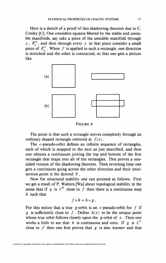
BULLETIN (New Series) OF THE AMERICAN MATHEMATICAL SOCIETY Volume 24, Number 1, January 1991
STATISTICAL PROPERTIES OF CHAOTIC SYSTEMS
D. S. ORNSTEIN AND B. WEISS
ABSTRACT. The theory of smooth dynamical systems and the theory of abstract dynamical systems (ergodic theory), although having the same roots, have for many years developed quite independently of one another. These theories have now matured to the point where they can be combined to shed light on the nature of chaotic behavior.
Introduction
1. Overview 1.1 Smooth dynamical systems 1.2 Abstract dynamical systems
1.2.1 Abstract systems 1.2.2 Concrete systems
1.3 Stationary processes 1.4 The picture from the point of view of abstract dynamical
systems 1.5 Smooth systems and hyperbolic structure 1.6 Isomorphism of smooth systems 1.7 a-congruence 1.8 a-congruence and smooth systems 1.9 Historical overview of isomorphism theory of chaotic sys
tems 1.10 More recent results in abstract isomorphism theory
2. a-congruence 2.1 Strong stochastic stability 2.2 Stability under random perturbations 2.3 Scaling time 2.4 Bernoulli flows and Markov processes 2.5 Long-term versus short-term behavior and simulation 2.6 Instability, or when a-congruence fails
Received by the editors June 5, 1988 and, in revised form, July 28, 1989. 1980 Mathematics Subject Classification (1985 Revision). Primary 28Dxx,
28Fxx, 58Fxx, 70D05. This work was supported in part by a grant from the National Science Founda
License or copyright restrictions may apply to redistribution; see https://www.ams.org/journal-terms-of-use
12 D. S. ORNSTEIN AND B. WEISS
2.7 Further directions for a-congruence 3. A survey of some abstract ergodic theory
3.1 The öf-distance 3.2 Entropy and a-entropy 3.3 Extremal processes 3.4 Very weak Bernoulli (VWB) 3.5 Finitely determined processes (FD) 3.6 Isomorphism theorems 3.7 Factors, ^-limits and the relativized theory
4. A survey of some smooth chaotic systems 4.1 Introduction 4.2 Geodesic flows 4.3 Anosov flows 4.4 Axiom A flows 4.5 Partially hyperbolic systems and billiards 4.6 Proving that smooth systems are Bernoulli 4.7 Smooth models for abstract systems
5. Proofs of the new results 5.1 Proofs for strong stochastic stability (§2.1) 5.2 Proofs for §2.4: Bernoulli flows and Markov processes 5.3 Proofs for §2.2: Random perturbations 5.4 Proofs for §2.5: Long-term versus short-term behavior 5.5 Proofs §2.3: Scaling time 5.6 Proofs for instability (§2.6) 5.7 Some proof for §3
Appendix by David Fried Bibliography
INTRODUCTION
Ergodic theory arose from an attempt to study the long-term1
statistical behavior of dynamical systems. The early successes of ergodic theory were Poincaré's recurrence theorem and Birkhoff s ergodic theorem. These results were proved without using the topological or differential structure that comes with a dynamical system. This led to abstract ergodic theory which studies measure-preserving transformations (in discrete) time and measure-preserving flows (in continuous time) on abstract measure spaces or, equiv-alently, abstract dynamical systems where all but the probability structure is abstracted out.
1 We watch our system forever.
License or copyright restrictions may apply to redistribution; see https://www.ams.org/journal-terms-of-use
STATISTICAL PROPERTIES OF CHAOTIC SYSTEMS 13
From another direction measure-preserving flows (or transformations) were introduced in order to model the stationary processes of probability theory. The level of abstraction of abstract ergodic theory is what allowed one to put dynamical systems and random processes into the same mathematical framework.
One of the problems concerning measure-preserving transformations that most interested ergodic theorists was the classification of the transformations that arise from independent processes—the Bernoulli shifts. The problem was considered important partly because of the role that independent processes have in probability theory and partly because of the simplicity of Bernoulli shifts. The first step in this direction was taken in 1958 when Kolmogorov and Sinai showed that not all Bernoulli shifts were isomorphic. This was done by transplanting the Shannon entropy from information theory to ergodic theory.
The problem was solved in 1970 when it was shown that Bernoulli shifts were completely classified by their entropy. The method used to prove this also gave a number of other results with the following common theme: There is a unique measure-preserving flow that is the most random flow possible (this is called the Bernoulli flow).
Independently of the development of abstract ergodic theory, Hopf, Anosov, Sinai, Pesin, etc. made great progress in elucidating the structure of specific systems. They showed that certain systems had hyperbolic structure, a, sharp form of "sensitivity to initial conditions," which could be used to prove things like ergo-dicity.
The proof of the isomorphism theorem for Bernoulli shifts did not use the independence property of Bernoulli shifts. Instead it rested on a property (FD, or finitely determined) derived from independence. It was observed that hyperbolic structure could be used to check FD. In this way many concrete systems were shown to be isomorphic to the Bernoulli flow. These are the only cases so far of chaotic (positive entropy) systems that have been determined up to isomorphism.
The main focus of this article will be the recent results that show that the isomorphisms produced by the abstract theory in some cases still preserve much of the concrete geometric structure that was abstracted away by abstract ergodic theory.
The first result along these lines was motivated by the purely topological results of the Anosov-Smale school about structural
License or copyright restrictions may apply to redistribution; see https://www.ams.org/journal-terms-of-use
14 D. S. ORNSTEIN AND B. WEISS
stability. Here isomorphism theory provides a fairly exact statistical analog of these results.
Further motivation came from the growing interest in chaos. A central issue here is understanding the phenomenon of systems that obey deterministic laws such as Newton's laws, but whose behavior seems to be random. Here isomorphism theory goes beyond sensitivity to initial conditions, which is a kind of randomness, by showing that in many cases the same system can be produced by Newton's laws or by a random mechanism based on coin flipping.
A much discussed question about chaos is whether randomness comes from the effects of small random perturbations (like thermal agitation) whose cumulative effect is large or from inherent deterministic laws. Here the isomorphism theory can show that, in certain cases, the process produced by small random perturbations (where effects in principle are cumulative) can also be produced by small random perturbations in the device through which we are observing the system. These latter effects are clearly not cumulative.
Chaos is sometimes studied by computer simulation. A result in this direction is the following: Bernoulli systems and (essentially) only Bernoulli systems have the property that long-term behavior can be modeled by a finite state machine (e.g., a computer) equipped with a roulette wheel.
Another question is whether long-term behavior is observable. It turns out that Bernoulli systems also have the property that their long-term behavior can be reconstructed from an observation of the system that lasts a (sufficiently long) finite time.
The plan of this paper is the following. §1 is a detailed introduction. §2 contains new results that re
late to chaos. These results are based on results in abstract er-godic theory and results about specific smooth systems. §3 gives the abstract background on which §2 is based, while §4 gives the smooth dynamical background. §5 gives the proofs for our new results. These are based on fairly long proofs which we do not reproduce but which can be found in the literature. The appendix by David Fried is about the relationship between structural stability and stochastic stability.
1. OVERVIEW
1.1 Smooth dynamical systems. For chaotic systems there is a very strong sensitivity to initial conditions, in the sense that
License or copyright restrictions may apply to redistribution; see https://www.ams.org/journal-terms-of-use
STATISTICAL PROPERTIES OF CHAOTIC SYSTEMS 15
arbitrarily small changes in the starting point eventually produce large changes in the trajectory. Individual trajectories are therefore not reproducible and the emphasis is placed, rather, on the overall features of ensembles of trajectories. In this spirit we form the phase space, which is the manifold M of all possible configurations of our system. If, for example, our system is a billiard ball moving with velocity 1 on a table, the phase space would be the three-dimensional manifold of all possible positions and directions of motion of the ball. The laws of physics tell us how a configuration changes and the time evolution of a configuration is represented by a trajectory, or orbit, in the phase space M. We can think of the time evolution, of the system as a whole, as a flow on M (i.e., a one-parameter family of transformations on M or the solution of an ordinary differential equation on M).
There are several approaches to the study of such flows, each of which focuses on certain features of the flow and ignores others. The features that one is concerned with are usually pinned down by the notion of equivalence. For example, the "qualitative theory of ordinary differential equations" initiated by Poincaré and extended by people like Sinai, Anosov, and Smale focuses on the topology of orbits. This is made precise by saying that flows on manifolds are equivalent if there is a homeomorphism between the manifolds that takes orbits to orbits. A stronger equivalence is also studied (in connection with structural stability) in which the manifolds are the same and the homeomorphism moves all points by less than a, thus preserving some of the geometry as well as the topology.
In many cases (e.g., Hamiltonian systems, billiard flows, geodesic flows, Axiom A attractors, etc.) there is an invariant measure on the phase space M that represents the probability that a configuration is in a certain set in the phase space. In this case we are able to study the statistical properties of the system.
Because a homeomorphism may take a set of measure 1 (probability 1 ) to a set of measure 0, it need not preserve the probability structure. Furthermore, a map that takes orbits to orbits need not preserve the parametrization of the orbits. Therefore, statements involving the evolution of a set E in M can get garbled under equivalence.
Because of the above, when studying the statistical properties of a dynamical system, we replace equivalence by isomorphism.
Definition of isomorphism. Two flows, ft acting on M, preserving a measure //, and ƒ acting on M, preserving /Z, are isomor-
License or copyright restrictions may apply to redistribution; see https://www.ams.org/journal-terms-of-use
16 D. S. ORNSTEIN AND B. WEISS
phic if there is an invertible measure-preserving map (j) between (M, n) and (M, ft) that takes orbits of ft to orbits of ft in a time-preserving manner, except possibly for a collection of orbits of measure 0 (i.e., <t>ft{x) - ft<f>(x) for all x except for an invariant set of measure 0).
1.2. Abstract dynamical systems.
1.2.1. Abstract systems. We can think of an equivalence class under isomorphism as an abstract dynamical system. More concretely we can define an abstract dynamical to be a one-parameter family ft of invertible measure-preserving transformations of an abstract (probability) measure space X where the map from XxR to X defined by (x, t) »-» ft(x) is measurable (i.e., the transformations are put together in a measurable way), and ft (ƒ, ) =
ftx+t2 '
1.2.2. Concrete systems. If we ignore sets of probability zero, then we can think of a concrete dynamical system as an abstract system together with a function P, where P is what we really see. If ft
is a flow on a manifold M, then P would be the identity function from M as an abstract measure space to M as a manifold. For an experimenter the function P might be just a finite-valued function defined on M that describes his possible observations.
1.3. Stationary processes. We have been describing measure-preserving flows in the context of dynamical systems. They can also arise from stationary processes like Markov processes.
The mathematical model for a continuous time stationary process taking values in a metric space M is a flow ft on an abstract measure space X and a function P from X to a metric space M. (P can be thought of as the result of an observation on X.)
We justify the model as follows: A stationary process (like a diffusion on M) is a measure on all possible paths.
If we start with ( ft, X, P) then for each x, the function from t to M, P(ft(x)), can be thought of as a possible path and X puts a measure on these paths.
2
See a formal description in the footnote at the beginning of §3.
License or copyright restrictions may apply to redistribution; see https://www.ams.org/journal-terms-of-use
STATISTICAL PROPERTIES OF CHAOTIC SYSTEMS 17
On the other hand, given a stationary process the paths, functions from t to M, form the measure space X, P tells us where the path is at time 0, and ft shifts the path by t.
Note that ( ft, X, P) can be thought of either as a stationary process or as a concrete system.
1.4. The picture from the point of view of abstract dynamical systems.
I. A central consequence of the isomorphism theory is the existence of a unique abstract system that is the most random abstract system possible. We call this system the Bernoulli flow or Bt. (The statement that Bt is the most random possible is, of course, not well defined and would not make sense if we did not identify isomorphic flows. However, we will now present theorems about Bt
that make this clear.3) In order to understand the nature of Bt, let us focus for a
moment on the case of discrete time. It seems clear that the most random kind of stochastic process is the process of independent random variables, in its simplest version the tossing of a fair coin. The corresponding transformation, the Bernoulli shift (\, \), is defined as the shift4 on Az with product measure where A has 2 points each of measure \ . (The general Bernoulli shift B(- ' Pt•' ' ' ) > Pi > 0 9 YsPi — 1 is defined similarly.) The simplest form of the isomorphism theorem says:
Theorem 1.4.1. B(- • -p. •• -pk) is isomorphic to #(• ••<?;• ••#/) if and only if £ p . log/?, = E Qj l°gtf; •
The class of independent processes is thus fairly simple from the point of view of isomorphism. A stronger theorem is the following.
Theorem 1.4.2. There is a flow Bt such that Bx is isomorphic to the Bernoulli shift (\ , \), and for any tQ, Bt is also a Bernoulli
shift; in fact we get all Bernoulli shifts by varying tQ.5 Bt is unique up to a constant scaling of the time parameter {i.e., if Bt is another
The results of this section may be found in [O 1]. 4Points in Az are doubly infinite sequences { a , } ^ . The shifted sequence is
the sequence {ât} , where ~ai = at_x , A = {ƒƒ, T} , a = H or a = T. The general Bernoulli shift is defined formally in §3.6.
5 More precisely, finite entropy shifts. For infinite entropy, see below. Also, note that Bt refers to a one-parameter family of transformations indexed by t while Bx and Bt refer to a single transformation in the family.
License or copyright restrictions may apply to redistribution; see https://www.ams.org/journal-terms-of-use
18 D. S, ORNSTEIN AND B. WEISS
flow such that for some t0, Bt is a Bernoulli shift, then there is a
constant c such that Bct is isomorphic to Bt).
II. To further justify our claim that Bt is the most random abstract flow possible, and to see that it occupies a unique place among chaotic flows, we will compare Bt with all the flows that could be considered random or chaotic. We will describe the class of random flows by eliminating the ones that are generally considered nonrandom. These are called completely predictable and are characterized by the property that all observations on the system are predictable in the sense that if we make the observation at regular intervals of time (i.e., every hour on the hour), then the past determines the future. (By an observation we simply mean a measurable function P on M—we can think of this as a stationary process.) It is not hard to prove that these are exactly the flows of zero entropy.
Theorem 1.4.3. Any flow ft that is not completely predictable {i.e., ft has positive entropy) has Bct as a factor. {The c's are those for which the entropy of Bct is not greater than the entropy of ft.) The only factors of Bt are Bct, 0 < c < 1.
The flow {gt, Y) is a factor of {ft, X) if there is a 0: X -> Y such that the inverse image of any measurable set is a set of the same measure and </>(fj(x)) = gt(<f>(x)) for all x except for an invariant set of measure zero.6 (If we insist that <f> is one-to-one and invertible, then ft and gt are isomorphic.) We could also think of a factor of ft as ft acting on an invariant sub-cr-algebra (these arise naturally from observations that do not generate).
Theorem 1.4.3 implies that if a system has any observation that is not predictable, then the set of processes arising from observations on the system includes all the processes that can arise from observations on Bt. Furthermore, it can also be shown that if ft
is not isomorphic to Bt, then there is some observation on f( that is more predictable than any observation on Bt in the sense that it is not VWB and not extremal. (VWB and extremal characterize the processes arising from Bt in terms of predictability and will be discussed in §3.) Furthermore, this observation cannot be approximated by observations on Bt in the sense of a-disparate (§2.6).
'An eigenfunction in our terminology is a rotation factor.
License or copyright restrictions may apply to redistribution; see https://www.ams.org/journal-terms-of-use
STATISTICAL PROPERTIES OF CHAOTIC SYSTEMS 19
III. One concrete realization of Bt is given by the following stationary process: Pick a > 0 and P > 0, with a/fi irrational. Flip a coin and wait a units of time if the outcome is heads (/? if the outcome is tails) before flipping again. The isomorphism theory implies that when we vary a, /?, and the bias of the coin, we get flows that are isomorphic to each other and to Bt (except for changing the unit of time, i.e., Bt —> Bct).
If ajP is rational we get the direct product of Bt and the flow of rigid rotations of the circle.
IV. So far, we have ignored the case of infinite entropy. (Note that smooth flows on compact manifolds must have finite entropy.) There are analogous results for infinite entropy that complete the picture.
If in our discussion of Bernoulli shifts we want to include all independent processes (i.e., define Bernoulli shifts as those transformations that arise from independent processes) then we must consider the cases when A is countably infinite or has a continuous part. In the countably infinite case we still have isomorphism if and only if E^logp, . = E ^ l o g ^ . . If 2>/k>8P,- = oo or if A has a continuous part, then we get the unique Bernoulli shift of infinite entropy B°° .
There is also a unique Bernoulli flow of infinite entropy B™ . B°° is the Bernoulli shift of infinite entropy for any £n. If ƒ
'0 U *0
is the Bernoulli shift of infinite entropy for some t0 then ft is isomorphic to B™ .
The only factors of B™ are B™ or Bct. The only factors of B°° are B°° or !?(•••/>,.•••)• B™ is a factor of any flow of infinite entropy. B°° is a factor of any transformation of infinite entropy. A concrete realization of Bf° is given by any Poisson process on the line.
V. The picture for flows not isomorphic to Bt is very complicated and poorly understood.
At one extreme we have the completely predictable (zero entropy) flows. These include billiards on a rectangular table with no obstacle and the horocycle flow on a manifold of negative curvature, and the rigid rotation of the circle.
The remaining flows, those that have some measurement that is not predictable (positive entropy), are generally considered chaotic
License or copyright restrictions may apply to redistribution; see https://www.ams.org/journal-terms-of-use
20 D. S. ORNSTEIN AND B. WEISS
and are characterized by positive Lyapunov exponents. Among the flows having some nonpredictable measurement are
those flows where all measurements are nonpredictable. These are called K flows or Kolmogorov flows (i.e., ft is K if it has no zero entropy factors; it is easy to see that Bt is K).
It was once hoped that the picture would be fairly simple, at least in discrete time. The hope was that all K transformations were Bernoulli shifts (Bernoulli shifts are easily seen to be K) and that every transformation was either K, or zero entropy or the direct product of K and zero entropy (the Pinsker conjecture). Both of these conjectures turned out to be false, both in continuous and in discrete time.
Theorem 1.4.4. There is a flow {transformation) that is not K, or zero entropy or the direct product of K and zero entropy.
Theorem 1.4.5. There are uncountably many nonisomorphic K flows {K transformations) of the same entropy. {For flows this means that they cannot be made isomorphic by a constant rescaling of time.)
0 entropy positive entropy all measurements not all measurements
are predictable are predictable
~ " ^ - ^ ^ C —Bernoulli
K
no measurements are predictable
FIGURE 1
1.5. Smooth systems and hyperbolic structure. Certain chaotic systems have what is called hyperbolic structure. For a diffeo-morphism D of a two-dimensional manifold, this would mean roughly, two invariant one-dimensional foliations, one of which expands exponentially under D while the other contracts exponentially. Hopf, Sinai, and Anosov used the hyperbolic structure to show that geodesic flow on manifolds of negative curvature was ergodic and in fact K. These results depended on delicate properties of the foliation and successive weakening of these conditions— Anosov flows, Axiom A flows, partially hyperbolic flows—were
In the popular terminology of chaos, positive entropy corresponds to sensitivity to initial conditions. This makes sense even if there is no invariant measure.
License or copyright restrictions may apply to redistribution; see https://www.ams.org/journal-terms-of-use
STATISTICAL PROPERTIES OF CHAOTIC SYSTEMS 21
studied. In addition, Sinai, Pesin, and many others found hyperbolic structure in a variety of specific systems. For example, Sinai [Si 4] found a partially hyperbolic structure in billiards with a convex obstacle and used this to prove ergodicity and the K property.
Hyperbolic structure was also used by Anosov [Ano 1] and Smale [Sm] to show that for certain systems, a small perturbation in the defining vector field did not change the topology of the orbits and did not change the geometry of orbits very much. More specifically there is a homeomorphism from the space on which the flow is defined, to itself that moves points by < e and takes orbits of the original flow to orbits of the perturbed flow in an order-preserving way.
1.6. Isomorphism of smooth systems. Combining hyperbolic structure and a variant of the isomorphic theorem of §1.4, we proved that the geodesic flow on a surface of negative curvature was isomorphic to Bt. This was the first nontrivial flow whose measure-theoretic structure was determined exactly. Furthermore, the proof gave a general method for checking if a concrete flow was Bt. This has led, over the years, to showing that a very large number of
o q
very different looking concrete flows are Bt. ' (In fact, the only nontrivial case where something is shown to be isomorphic to a Bernoulli shift or flow depends on the isomorphism theorem.)
Here is a small sampling of the flows that have been shown to be isomorphic to Bt or ~Bt, the direct product of Bt and the flow that rotates the circle. Geodesic flow on a manifold of negative curvature of any dimension is Bt. Axiom A attractors are Bt or 'Bt [Rat 1, Bun]. The motion of a billiard ball on a table with a convex obstacle is Bt, [GO] a model for the Lorentz attractor is Bt [Rat 2]. The following theorem of Pesin [Pe] is especially striking: Theorem 1.6.1. Let ft be a smooth flow on a three-dimensional compact manifold that preserves a smooth10 invariant measure.
o
We can get a better feeling for the result that all geodesic flows on all surfaces of negative curvature are isomorphic (up to rescaling time) by contrasting it with the following result: Horocycle flows on surfaces of negative curvature are isomorphic (up to rescaling of time) only if the surfaces are the same (isometric). This means that the picture does not necessarily simplify when we identify isomorphic flows, and that a measure-preserving flow on an abstract measure space can, in principle, contain smooth information (we can reconstruct the surface) [Fe 0], [Ot].
o Many such examples can be found in [Si 7, Part II]. Absolutely continuous with respect to Lebesgue measure.
License or copyright restrictions may apply to redistribution; see https://www.ams.org/journal-terms-of-use
22 D. S. ORNSTEIN AND B. WEISS
After ignoring an invariant set of measure zero, we have that: Any ergodic component on which ft is not completely predictable has positive measure and on each such component ft is either Bt or
V Bt can also arise from a variety of stationary processes. A few
examples are: A semi-Markov flow (where the particle remains in each of a finite number of states—st for a fixed time t{ and then jumps according to the spin of a roulette wheel) is Bt or Bt. In particular, if the process has two states, changes states with probability £, and if tx/t2 is irrational, then the process is Bt
[O 5]. Poisson processes, continuous time Markov processes on a finite number of states, or Brownian motion with reflecting barriers (so it remains in a finite interval or square) are B™. [McCSh, AdShSmo]
Here are a few results for discrete time. In an algebraic context we have the beautiful result of Katznelson, Lind, and Miles and Thomas: [Katz, Lin, MiTn 1, 2, 3]. Any ergodic automorphism of a compact Abelian group is isomorphic to a Bernoulli shift. For one-dimensional maps we have that the natural extension of the continued fraction transformation is Bernoulli; [Smo] the natural extension of the maps ax (I - x), for those a for which there is an absolutely continuous invariant measure, is Bernoulli [Led].
Because of the large variety of systems isomorphic to Bt or Bt, we conjecture that most chaos is Bernoulli. To the extent that this is true, the diversity that we see would come from different measurements on the same abstract system. Furthermore, the diversity would be tamed because there are only a countable number of processes that can arise from observations on Bt (if we identify measurements that differ by a small amount except on a small part of the state space). Thus at the outer limit of randomness we get an extra amount of simplicity.
1.7. a-congruence. Because very different systems can be isomorphic, we propose studying a stronger kind of isomorphism which takes into account both the geometry and the statistical properties.
Definition of a-congruence. We will say that two measure-preserving flows ft and ft on the same compact metric space M are
Compactness is essential. Any measure-preserving flow can be modeled by a C°° flow, preserving a smooth invariant measure, even on a two-dimensional manifold which is, of course, noncompact [ArOW].
License or copyright restrictions may apply to redistribution; see https://www.ams.org/journal-terms-of-use
STATISTICAL PROPERTIES OF CHAOTIC SYSTEMS 23
a-congruent if they are isomorphic and the map 0 from M to M that implements the isomorphism moves the points in M by < a except for a set of points in M of measure < a.
If we agree that we cannot distinguish points in M that have distance < a, and if we are willing to ignore events of probability less than a (experimental error), then a-congruent flows are indistinguishable.
Assuming ergodicity for the flow, the ergodic theorem will imply that if two flows are a-congruent, then, almost surely, orbits of corresponding points in M are within a of each other except for a set of times of density < a . Thus a-congruent flows have essentially the same collection of orbits with the same probability distribution.
We will also define a-congruence in a more general context. If ft and ft are flows on abstract measure spaces X and X and P (and P) are functions from X(X) to a metric space then:
Definition. (ft,X,P) and (ƒ, ,X,ÎP) are a-congruent if there is an invertible measure-preserving </>, </>ft(x) = ft<t>{x) a.e. and d(P(x), ~P{(j)x)) < a except for a set of measure < a (d denotes distance in the metric space).
An alternative wording of the above definition is the following: ( ft, X, P) and ( ft, X , P) can be jointly modeled by a third system (fl, X', P' U 7 ) where (a) P' (and 7 ) generate the entire a-algebra under f[ , (b) {f[, X', P') (and (j£, X\ ?')) give the same concrete systems as (ft, X, P) (and (ft, X, P)), and (c) T' and P' differ by less than a except on a set of measure < a . This says that our systems differ by a small change in the function that tells us what we see.
P and P can be thought of as the functions that make the abstract system (ft, X) and (ft, X) into concrete systems.
1.8. a-congruence and smooth systems. One kind of a-congruence result is a statistical version of structural stability. Consider, for example, a rectangular billiard table with a convex obstacle. Pick a > 0. Now perturb the obstacle so that the shape and the curvature change by a small amount (depending on a ) . The original and the perturbed billiard flow will then be a-congruent. (We may have to rescale time in one of the flows, by a small amount, i.e., change ft to fct, |1 - c\ < a , c is a constant.) We also
License or copyright restrictions may apply to redistribution; see https://www.ams.org/journal-terms-of-use
24 D. S. ORNSTEIN AND B. WEISS
get an a-congruence result for essentially the same systems and perturbations for which structural stability holds. In addition, we get a-congruence results for some systems that are not structurally stable.
The main difference between structural stability and the above a-congruence result is that the homeomorphisms in structural stability preserve the topology while the map in a-congruence preserves probabilities. Moreover, in a-congruence the parametriza-tion of orbits is preserved (or rescaled by a constant) and therefore corresponding sets evolve in the same way. On the other hand we lose all information about events of probability zero.
Another stability result says that in certain cases adding noise to a system will have the same effect as leaving the system alone but adding noise to the device through which we view the system. Suppose we add noise to an axiom A diffeomorphism, D, by after applying D to a point x, jumping with uniform distribution in a sphere of small radius around D(x). Our result says that there is a viewer whose state changes randomly but independently of D, and where the point that we see when looking through the viewer (which depends on the point we are looking at and the state of the viewer) is with high probability close to the point we are looking at. If we look at the unperturbed diffeomorphism through this viewer, we see our perturbed system exactly (all joint probabilities are the same). The interest in this result lies in the fact that the effects of the first perturbations are clearly cumulative, while the effects of the viewer are not since the viewer does not interfere with D, and only misreads a point slightly.
Another a-congruence result says that the randomness of systems isomorphic to Bt manifests itself in a more concrete way. Consider billiards with a convex obstacle. Pick a > 0. We can define a process on the same table, whose mechanism is governed by tossing a (biased) coin, that is a-congruent to billiards. The process can be described as follows: Our ball will always be at one of a finite number of points on the table. It will stay at each point p for time t(p) and will then jump to one of a pair of points according to the flip of our biased coin. (The pair of points depends on p.)
If we think of the function that implements the above a-congruence as a device or viewer which looks at the billiard ball and according to its position and velocity sees one of the special points on the table, then our result could be phrased as follows: There is a viewer that is deterministic and does not distort by > a for a
License or copyright restrictions may apply to redistribution; see https://www.ams.org/journal-terms-of-use
STATISTICAL PROPERTIES OF CHAOTIC SYSTEMS 25
collection of configurations of probability > 1 - a and when we look at the billiards through this viewer we see a ball that moves according to the flips of the coin.
An additional a-congruence result says that the long-term behavior of a Bernoulli flow on a manifold is finitely accessible: There is an algorithm that takes an observation of our system for a sufficiently long, but finite, interval of time and produces a stationary process that could have been produced by watching our system (forever) through a viewer whose state changes randomly but with high probability, distorts very little.
1.9. Historical overview of isomorphism theory of chaotic systems. Isomorphism theory for chaotic systems began in 1958 when Kolmogorov and Sinai introduced the concept of entropy (§2.4) into ergodic theory and used it to solve a long-standing problem by showing that not all Bernoulli shifts were isomorphic. They showed that the entropy of B(p{, p2, p3) was p{ logp{ +p2 logp2+ p3 log/?3, etc. and that shifts of different entropy could not be isomorphic [Ko ,1, Ko 2, Si 1].
In 1962 Sinai [Si 2] showed, in discrete time, that a Bernoulli shift was a factor of everything of equal or larger entropy. In 1967 Adler and Weiss [AdW 1,2] proved an isomorphism theorem for automorphisms of the 2-torus.
Entropy also gave the break up into completely predictable and not completely predictable and completely unpredictable [Ko 1, Ko 2, Si 1].
On the concrete side Sinai and Anosov showed that a large class of systems (including billiards with obstacles) had a "good hyperbolic structure" and used this to show that they were completely unpredictable [Si 3, Ano 1, Si 4].
Anosov also used hyperbolic structure to show that these systems were stable in a topological (rather than statistical) sense (structural stability) [Ano 1].
In 1970 Ornstein showed that Bernoulli shifts of the same entropy were isomorphic [O 2]. The method was different from the Adler-Weiss proof or the Sinai proof.
By a different set of ideas Ornstein showed that the completely unpredictable class contained more than the Bernoulli shifts and that not every transformation was the direct product of a completely unpredictable and a completely predictable transformation (the Pinsker conjecture) [O 7, O 8, O 9, OSh].
License or copyright restrictions may apply to redistribution; see https://www.ams.org/journal-terms-of-use
26 D. S. ORNSTEIN AND B. WEISS
By the method used to prove the isomorphism theorem for Bernoulli shifts, Ornstein showed that Bernoulli shifts can be embedded in a flow and there is a unique Bernoulli flow Bt which strings together all of the Bernoulli shifts [O 6], that Bt was a factor (modulo scaling) of any flow that was not completely predictable (the continuous time extension of Sinai's 1962 result), and that the only factor of Bt is Bct, 0 < c < 1 [O 1],
The connection with concrete systems was made when Ornstein and Weiss showed that the geodesic flow on a surface of negative curvature is isomorphic to Bt [OW 3]. Since then it was shown that a large class of specific flows was isomorphic to the Bernoulli flow. This was done by using the hyperbolic structure (elucidated by Sinai-Anosov-Pesin and others) to check a criterion, VWB (see §2.6), which makes the isomorphism theorem work [GO, Pe, Rat, Bun].
In many cases the isomorphisms produced by the theory do not move points very much and these are the results about a-congruence and stability that we will focus on in the next section.
1.10. More recent results in abstract isomorphism theory. We have so far described the history of the isomorphism results that we have been concerned with in this paper. The subject, however, does not end here and some of the deepest results in isomorphism theory are outside the scope of this paper. We will now try to give the reader a hint of these results.
Thouvenot [Tho 1, Tho 2] introduced the idea of relativizing with respect to a factor, and showed that the isomorphism arguments could be relativized. This gave criteria for when a factor had an independent Bernoulli complement. Our results involving viewers whose state changes use this theory.
A sample result of the Thouvenot theory is that a factor of the direct product of a zero entropy and a Bernoulli is again of that form.
Thouvenot's theory^can also be obtained by substituting a different metric for the d metric of §3 [Rud 2]. Feldman introduced yet another metric and initiated the study of measure-theoretic equivalence where one weakens the definition of isomorphism by allowing orbits to map to orbits with a time change that varies from point to point along the orbit [Fe 1]. Ornstein, Rudolph, and Weiss modified the isomorphism machinery to accommodate Feldman's
License or copyright restrictions may apply to redistribution; see https://www.ams.org/journal-terms-of-use
STATISTICAL PROPERTIES OF CHAOTIC SYSTEMS 27
metric [ORudW]. This direction culminates in Rudolph's equivalence theory [Rud 2].
Rudolph has a very deep theorem about the Bernoulliness of compact extensions of a Bernoulli shift [Rud 3, Rud 4]. The Bernoulliness of many concrete examples relies on this result. Rudolph's compact extension result together with an isomorphism theorem for actions of a skew product of the integers and a compact group allows him to classify12 the factors of a Bernoulli shift with finite fibers [Rud 5]. There are results that indicate that the classification of all factors of a Bernoulli shift has much of the complexity of the general classification problem for transformations [O 10].
Ornstein and Weiss [OW 2] developed an isomorphism theory for actions of a general amenable, unimodular group. This builds on Rudolph's isomorphism theory for Z skew compact group, the isomorphism theorems for Zn and Rn , Feldman's r-entropy [Fe 2], and new proofs of the Shannon-McMillan theorem.
The above results build on the original proof of the isomorphism theorem for Bernoulli shifts but in many cases there is a new level of intricacy and ingenuity.
In a different direction, Keane and Smorodinsky [KeSmo] have proved a version of the isomorphism theorem for Bernoulli shifts where the codes are finitary. The Adler-Weiss isomorphism theorem for toral automorphisms was also finitary and there is now a large and active area concerned with various kinds of finitary codes.
Lastly we should mention that there is a rich and beautiful collection of counterexamples. In particular we mention Rudolph's theory of "minimal self joinings," a systematic method of constructing certain kinds of examples [Rud 6].
2. a-CONGRUENCE
2.1. Strong stochastic stability. The individual orbits of chaotic systems are highly unstable but in certain cases the system as a whole will be stable. To discuss the stability of a certain system, we must specify the allowed perturbations and give a way of measuring their size. We must also specify the sense in which we want the perturbed system to be close to the unperturbed system. In all of our results "close" will mean a-congruent, for small a. Since
1 We want an isomorphism of the whole system that takes corresponding factors to each other.
License or copyright restrictions may apply to redistribution; see https://www.ams.org/journal-terms-of-use
28 D. S. ORNSTEIN AND B. WEISS
we have results for many kinds of perturbations, we will make a definition that focuses only on the sense of closeness.
Definition. ft is stochastically stable under a certain kind of perturbation if given ft and a > 0 and if ft is a small enough perturbation (of the right kind) of ft there is a constant c, 11 -c\ < a and ft and fct are a-congruent.
( ft and ft cannot be isomorphic unless the entropies are the same, c is the unique scaling of time that makes the entropies of ft and ft the same.)
We will postpone for the moment a discussion of the kinds of systems and the kinds of perturbations for which we have stochastic stability and focus on what stochastic stability tells us, by comparing it with a celebrated kind of topology stability called structural stability (or Q stability). These topological stability results say that if ft is a flow of a certain kind on a manifold M, then given ft and a > 0, if ƒ t is a small enough perturbation of the right kind, there is a homeomorphism of M to M that takes orbits of ft onto orbits of ƒ t and moves points by < a.
The conclusion of stochastic stability differs from that of structural stability in three ways: The homeomorphism is replaced by an invertible measure-preserving map. The map takes orbits rigidly onto orbits (i.e., after rescaling time, the map is an isomorphism). Instead of moving all the points by < a, there is a set of points of measure > 1 - a that are moved by < a. (We will discuss the necessity of this weakening in Remark 3 below.)
For example, if the perturbation only changes the speed of the flow and does this in a nonconstant way, then the structural stability homeomorphism could be the identity while the stochastic stability map must permute orbits.
Before giving a discussion of a general class of systems and perturbations for which we have stochastic stability, we will give some concrete examples:
Theorem 2.1.1. Let ft be the geodesic flow on a manifold L of negative curvature. Fix a > 0. If ƒ\ is the geodesic flow on L resulting from a small {given a) change in the Riemannian structure on L ,l3then ft and fct are a-congruent where \c-\\ < a.
The corresponding metric tensors should be C -close.
License or copyright restrictions may apply to redistribution; see https://www.ams.org/journal-terms-of-use
STATISTICAL PROPERTIES OF CHAOTIC SYSTEMS 29
(Note that a geodesic flow on L is really a flow on M, the unit tangent bundle to L, and preserves the Riemannian measure on M).
Theorem 2.1.2. Let ft be the billiard flow on a square table with a convex obstacle. Fix a > 0. If f t is the flow resulting from a small (given a) perturbation in the obstacle and its curvature, then ft will be a-congruent to fct where | 1 - c\ < a.
(Note that ft (and ft) is a flow on a three-dimensional manifold M, consisting of positions on the table and directions; ft
(and ft) preserve Lebesgue measure.) A general result is that we have stochastic stability for a class of
situations that include essentially the same systems and perturbations for which we have structural stability.,14 We will devote the rest of this section to a more careful statement of the above claim [Ma l ,Ma2] .
A result (due mainly to Smale and Mané) characterizes the flows that are structurally stable under C1 perturbations of the defining vector field as axiom A systems (with some extra technical conditions). Axiom A systems are, except for a set of measure zero, a finite union of axiom A attractors, and we will therefore focus on the stochastic stability axiom A attractors. These are discussed in §4.4 but we will summarize some points needed for this discussion.
Axiom A attractors are smooth flows defined on a manifold M or a subset Q of ¥ . These flows are a generalization of geodesic flows on a manifold of negative curvature where Anosov first proved structural stability.
C2 axiom A attractors do have a canonical invariant measure, the Sinai-Bowen-Ruelle measure (or SBR measure). This measure is believed to be physically relevant. When we consider an axiom A attractor we will always endow it with its SBR measure.
To make sense out of stochastic stability, both the flow and its perturbation must have an invariant measure. A C flow that is sufficiently close C1 to an axiom A attractor is itself an axiom A attractor and therefore has an SBR measure.
Definition of strong stochastic stability (SSS). We will say that a C2 axiom A attractor, ft on M, is strongly stochastically stable
It is hoped that stochastic stability is a much more general phenomenon than structural stability, see §2.7.
License or copyright restrictions may apply to redistribution; see https://www.ams.org/journal-terms-of-use
30 D. S. ORNSTEIN AND B. WEISS
or SSS if given a > 0 : if ƒ t is a C flow on M that is sufficiently close C1 to ft, then ƒ, and fct are a-congruent for | c - 1| < a .
We turn to the question: Which C2 axiom A attractors are SSS?
We first note that C axiom A attractors come in two flavors, that is, we have the following dichotomy.
Type 1. ft is a suspension. This means that there is a nontrivial eigenfunction (i.e., a function g from M to the circle such that
#(ƒ*(*)) = Ryt(s(x)) w h e r e ^ y r i s r o t a t i o n by J") • I f ƒ, h a s a
measurable eigenfunction, then it has a continuous one and is not topological^ mixing. ft is isomorphic to the direct product of the Bernoulli flow and the flow that rotates the circle.
Type 2. ft has no measurable eigenfunction. ft is topologically mixing. ft is isomorphic to the Bernoulli flow.
The relevance of the above discussion is that a flow of type 1 is not isomorphic to a flow of type 2. It is also easy to see that if ft
is type 1, then we can make an arbitrarily small perturbation, ƒ t , such that ft is type 2.
This means that a type 1 flow cannot be SSS and a type 2 flow that is the C1 limit of type 1 flows cannot be SSS.
Our theorem is that the above are only obstructions to SSS.
Theorem 2.1.3. A C axiom A attractor is SSS if and only if it is not the C limit of C suspensions.
The question now arises: Can an axiom A attractor be a Cx
limit of suspensions but not a suspension itself? David Fried clarified this situation for us and the complete answer is given in the Appendix. Here is part of the story: It can happen, but it cannot happen if ft is Anosov of dimension < 4. It cannot happen if the expanding and contracting foliations are not jointly integrable. It cannot happen if àimH{(U, JR) = 1 (U being a small open neighborhood of the attractor).
Theorem 2.1.4. If ft is an axiom A attractor that is not a suspension, even if it is a C{ limit of suspensions, then one still has a lot of stability : either the perturbation ft is a-congruent to fct or to Rtxfct, | c - l | < a .
Rt x fct acts on the product of the circle and the manifold. Here Rt is the flow that rotates the circle with small period and
License or copyright restrictions may apply to redistribution; see https://www.ams.org/journal-terms-of-use
STATISTICAL PROPERTIES OF CHAOTIC SYSTEMS 31
the isomorphism <j> takes a point (y9x), where y is on the circle and x is in M, to a point x in M . x and x' are closer than a with probability > 1 - a (i.e., we are using the second definition of a-congruence).
The a-congruence to Rt x fct could be pictured as follows: We could think of Rt as a viewer whose state or condition changes cyclicly. When we look at a point x in M through the viewer, we see a point x'(x = </>(y 9 x)) in M. x depends only on x and the state y of the viewer. When we look at fct through the viewer, we see exactly ft. We could recover the point we are looking at and the state of the viewer from the orbit that we see, i.e., there is an inverse viewer (whose state does not change).
We could, of course, also think of the a-congruence between ft
and fct as being implemented by a viewer whereby we look at a point x in M and see a point (f)(x) in M. Thus if we watch fct
through this viewer, we will see ft (and looking at ft backwards through this viewer we see f c t ) .
The main point of statistical stability is that the effect o f a C{
perturbation is in principle cumulative, whereas the distortions produced by a viewer are clearly not cumulative.
Remark 1. The difficulties associated with types 1 and 2 do not occur in the theory of structural stability because we do not insist in this theory that orbits map to orbits rigidly. If we gave up on this requirement in the statistical case, the difficulty would similarly disappear.
Proposition. Let ft be the flow on an axiom A attractor M. Then — 2 i
given a> 0, if ft is a C flow, sufficiently close C to ft, there is an invertible measurable15 map from M to M that takes orbits to orbits and moves all points by < a except for a set of measure < a.
Remark 2. The reason we do not strengthen SSS by requiring that (f) move all points by < e is that for axiom A flows there is only one orbit of the perturbed system that is uniformly close to a given orbit of the original system. If, for example, the perturbation only changes the speed of the flow, then each orbit must map onto itself. It is easy to see that this cannot be done rigidly and measurably unless the speed change is very special. If we strengthened the
If (j) is not an isomorphism, it cannot take an invariant measure to an invariant measure.
License or copyright restrictions may apply to redistribution; see https://www.ams.org/journal-terms-of-use
32 D. S. ORNSTEIN AND B. WEISS
conclusion of Theorem 1 when L has dimension 2, then L and its deformation would have to be isometric. This follows from a theorem of Otal [Ot]. Remark 3. In Theorem 2.1.2 it is important not to change the curvature very much. If we approximate the boundary of our obstacles arbitrarily well by polygons, then (*), after ignoring a collection of orbits of total probability zero, any orbit of the original flow and any orbit of the perturbed flow will be D apart on the average, where D is the average distance between points in the state space. (This is because the perturbations have entropy 0.) If we take sufficiently good smooth approximations to the polygon, (*) will still hold but our perturbation will now have positive entropy and will even be Bernoulli.
Here are a few general comments on the meaning of SSS. Two flows that are close in the C1-topology behave in a simi
lar way for some finite amount of time. The closer they are, the longer this finite amount becomes, but it remains finite. Thus in a sense, knowing {ft} up to a small error in C1 determines only the short-term behavior of the system. The SSS of ft means that the approximate short-term behavior actually determines the long-term behavior arbitrarily far out in time (even though the individual orbits are sensitive to initial conditions).
The number of different ft on M that are SSS is severely limited: For fixed a, there are only a countable number of different ft up to «-congruence.
Stability properties are important from the point of view of experimentation or simulation. Because we can never duplicate an experiment exactly and in general we do not even know the theoretical model exactly, we need some stability properties in order to observe, simulate, or experiment with a system. Remark 4. We also have an a-congruence theorem for axiom A diffeomorphisms, but because we cannot scale time the result is not as clean.
Theorem 2.1.5. Let f be a connected axiom A attractor on M — 2
and pick a > 0. If f is a C diffeomorphism on M that is sufficiently close in C1 to ƒ, then either ƒ is a-congruent to the direct product of ƒ and a Bernoulli shift, or ƒ is a-congruent to the product of ƒ and a Bernoulli shift.
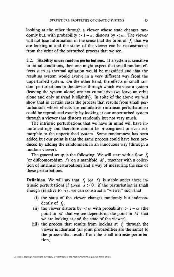
We can interpret this result as saying that one of the diffeomorphisms can be reproduced exactly (ignoring probability 0) by
License or copyright restrictions may apply to redistribution; see https://www.ams.org/journal-terms-of-use
STATISTICAL PROPERTIES OF CHAOTIC SYSTEMS 33
looking at the other through a viewer whose state changes randomly but, with probability > 1 - a, distorts by < a. The viewer will not lose information in the sense that the orbit of ft that we are looking at and the states of the viewer can be reconstructed from the orbit of the perturbed process that we see.
2.2. Stability under random perturbations. If a system is sensitive to initial conditions, then one might expect that small random effects such as thermal agitation would be magnified and that the resulting system would evolve in a very different way from the unperturbed system. On the other hand, the effects of small random perturbations in the device through which we view a system (leaving the system alone) are not cumulative (we leave an orbit alone and only misread it slightly). In spite of the above we will show that in certain cases the process that results from small perturbations whose effects are cumulative (intrinsic perturbations) could be reproduced exactly by looking at our unperturbed system through a viewer that distorts randomly but not very much.
The intrinsic perturbations that we have in mind will have infinite entropy and therefore cannot be a-congruent or even isomorphic to the unperturbed system. Some randomness has been added but our point is that the same process could have been produced by adding the randomness in an innocuous way (through a random viewer).
The general setup is the following: We will start with a flow f (or diffeomorphism ƒ) on a manifold M, together with a collection of intrinsic perturbations and a way of measuring the size of these perturbations.
Definition. We will say that ft (or ƒ) is stable under these intrinsic perturbations if given a > 0 : if the perturbation is small enough (relative to a), we can construct a "viewer" such that
(i) the state of the viewer changes randomly but independently of ft,
(ii) the viewer distorts by < a with probability > 1 - a (the point in M that we see depends on the point in M that we are looking at and the state of the viewer),
(iii) the process that results from looking at ft through the viewer is identical (all joint probabilities are the same) to the process that results from the small intrinsic perturbation,
License or copyright restrictions may apply to redistribution; see https://www.ams.org/journal-terms-of-use
34 D. S. ORNSTEIN AND B. WEISS
(iv) the viewer does not involve extra information in the sense that the orbit of ft that we are looking at and the state of the viewer can be reconstructed from the orbit of the perturbed process that we see.
Note, (iv) also means that ft and the viewer produce our process in a nonredundant way. As well it means that ft together with the viewer is, measure theoretically, the minimal mechanism capable of producing our process (the intrinsic perturbation).
Our viewer can be modeled as follows: The states of the viewer will form a measure space V. A measure-preserving flow on V, denoted by vt, will govern the way that the state of the viewer changes with time. The dynamical system that results from ft and the viewer will be the direct product of vt and ft: (vtxft, Vx M). (The measure on V x M is a product measure.)
The way the viewer distorts will be described by a function Q from V x M to M. If we look at x in M through the viewer and the state of the viewer is w in V, then the point in M that we see will be Q(w, x). The reliability of the viewer will be the expected distance between x and Q(w, x) (using product measure on V x M). In addition Q will generate under vt x ft
so that Q does not lose information. An intrinsic perturbation can be thought of as a stationary pro
cess with values in M or a measure on M, the collection of all paths in M. We model this by (st, M, P) where st shifts each path in M by t and P is the function from M t o M that tells us where the path is at time 0.
Restating our previous definition in the language of a-congru-ence, we get:
Definition. ft is stable under intrinsic random perturbations of a certain kind if, given a > 0, any sufficiently small intrinsic perturbation (denote the resulting process by (st, X, ~P) where X is the space of paths and P tells us where the path is at time 0) is a-congruent to the direct product of ft and some flow vt (call it (vt x ft, V x M)) relative to the functions 7 and Ö where Q(w, x) = x, w in V and x in M.
This agrees with our previous definition if we let our viewer be (vt x ft, V x M, Q) where Q is the image of 7 under the a-congruence.
License or copyright restrictions may apply to redistribution; see https://www.ams.org/journal-terms-of-use
STATISTICAL PROPERTIES OF CHAOTIC SYSTEMS 35
An alternative wording of our definition is the following: In {vt x ft, V x M, Q) we can make a small change in Q (obtaining Q), and {vt x ft, V x M, Q) models our intrinsic perturbation exactly and Q generates under vt x ft.
(A) Our first example will concern a diffeomorphism (ƒ, M) because it is easiest to describe. The perturbation will be a Markov process on M obtained as follows: Apply ƒ to x and then jump with uniform distribution in a ball of radius r around f(x). Then apply ƒ again to the resulting point, etc. This will give a unique probability measure on the space X of paths through M which is invariant under the shift S. Our model for this Markov process is (S, X, JP) where P tells us where a path is at time 0. The size of the perturbation is measured by r.
Theorem 2.2.1. An axiom A attractor that is Bernoulli is stable under the above kind of intrinsic random perturbation.
(B) Our next example concerns perturbations that are not arbitrarily small but occur very rarely. All Bernoulli flows are stable under such perturbations (think of a billiard table with a convex obstacle that is bumped once in a great while).
Start with a stationary process that alternates between long random periods of quiet (all at least of size L) and short active periods of fixed size A. During the quiet periods we flow using ft(x). If we are at x at the start of an active period, then we diffuse for a period of time equal to A to a new point xA which has an absolutely continuous distribution /u(x) which we assume dominates a fixed constant times the volume element in a ball of fixed radius around x. The nature of the diffusion is not relevant. From xA
one continues to flow with ft until the end of the next quiet period. Fixing the //(x)'s and measuring the size of the perturbations by 1/L we have:
Theorem 2.2.2. Every Bernoulli flow on a compact manifold pre-serving a smooth invariant measure is stable under the above intrinsic perturbations.
(C) There is a continuous time analog to Theorem 2.2.1 but it is technically harder to describe because the perturbation takes place infinitesimally (i.e., our intrinsic perturbation results from a diffusion).
License or copyright restrictions may apply to redistribution; see https://www.ams.org/journal-terms-of-use
36 D. S. ORNSTEIN AND B. WEISS
One formalism goes as follows. To the flow ft we associate its differential equation
*P-nw. dt
where F is a C2-vector field on M. The random perturbation will be given by wt = [w], . . . , wt ) , the standard d-dimensional Brownian motion, and C2-vector fields on M, Xl9 ... , Xd. The diffusion process xt can be described by a stochastic differential equation
d
dxt = V{xt) dt + Y, xMt) dw\ 1=1
or by an infinitesimal generator
(*) L=V + \j^XiXi.
Corresponding to the transition probability measure fi{x) above, we now have P(t,x,dy) which describes the distribution of a point at time t that was at x at time 0. If L is a nondegener-ate elliptic operator, then these transition probabilities P(t, x9 •) have a unique invariant measure on the manifold, say v, and then a shift invariant measure Pv is defined on the space of all continuous maps from R to M, X = C(R, M), so that
Pu({xteA}) = u(A) for all f
and
= / • • • / P(t{ - t0, u0, du{)P(t2 -tl9ux, du2)
'"P(tk-tk_l9uk_l9 duk)du{u0)
for t0< tx"- < tk and sets A0, . . . , An c M, where the integration is over all ute An 0 < / < R.
An invariant measure // for the flow ft also gives a measure on X , say dm, which is described in a similar way by saying that m({tx G A0, . . . , xt e Ak}) equals the // measure of the set of those points u0 in A0 such that ft_t (uQ) G At. In a sense this is unnecessary for /u, since X with dm can be identified, up to a null set, with M itself. However, for the Markov process this trajectory space is essential and it is there that we will describe the stability. We metrize X by giving it the topology of uniform
License or copyright restrictions may apply to redistribution; see https://www.ams.org/journal-terms-of-use
STATISTICAL PROPERTIES OF CHAOTIC SYSTEMS 37
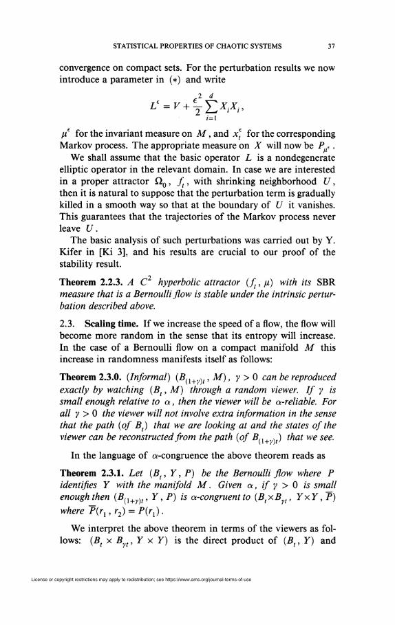
convergence on compact sets. For the perturbation results we now introduce a parameter in (*) and write
fi€ for the invariant measure on M, and x] for the corresponding Markov process. The appropriate measure on X will now be P e.
We shall assume that the basic operator L is a nondegenerate elliptic operator in the relevant domain. In case we are interested in a proper attractor Q0, ft, with shrinking neighborhood U, then it is natural to suppose that the perturbation term is gradually killed in a smooth way so that at the boundary of U it vanishes. This guarantees that the trajectories of the Markov process never leave U.
The basic analysis of such perturbations was carried out by Y. Kifer in [Ki 3], and his results are crucial to our proof of the stability result.
Theorem 2.2.3. A C2 hyperbolic attractor (ft, //) with its SBR measure that is a Bernoulli flow is stable under the intrinsic perturbation described above.
2.3. Scaling time. If we increase the speed of a flow, the flow will become more random in the sense that its entropy will increase. In the case of a Bernoulli flow on a compact manifold M this increase in randomness manifests itself as follows:
Theorem 2.3.0. {Informal) (B,x+y)t, M), y > 0 can be reproduced exactly by watching (Bt, M) through a random viewer. If y is small enough relative to a, then the viewer will be a-reliable. For all y > 0 the viewer will not involve extra information in the sense that the path (of Bt) that we are looking at and the states of the viewer can be reconstructed from the path (of Bn+y\t) that we see.
In the language of a-congruence the above theorem reads as
Theorem 2.3.1. Let (Bt, Y, P) be the Bernoulli flow where P identifies Y with the manifold M. Given a, if y > 0 is small enough then (2?,j w, Y, P) is a-congruent to (BtxB , YxY,7) where T(rx, r2) = P{rx).
We interpret the above theorem in terms of the viewers as follows: (Bt x B t, Y x Y) is the direct product of (Bt, Y) and
License or copyright restrictions may apply to redistribution; see https://www.ams.org/journal-terms-of-use
38 D. S. ORNSTEIN AND B. WEISS
(Byt, Y). P allows us to identify (Bt, Y) and (Bt, M). Our viewer is (B t, 7 ) . If Q is the image of P under the a-congru-ence, then Q(r{, r2) tells us what we see when we look at r{ in M and the viewer is in state r2(r2 e Y). a-congruence implies that Q is close to P and thus our viewer is reliable.
We can also slow Bt by looking at it through a deterministic viewer but we cannot reconstruct the orbit we are looking at from the orbit that we see.
The above theorem can fail dramatically in the non-Bernoulli case. For example, if ft rotates the unit circle by t, then any orbit of ft and any orbit of fct will differ by \ on the average, no matter how close c is to 1, i.e.,
^ f \td-ctd\dt-> i . 1 Jo
There is also a K flow ( ft, X, P) such that the orbits produced by ( ft, X, P) and the one produced by ( fct, X, P), c ^ 1, differ in the same quantitative sense: There is an a > 0 (that does not depend on c) and
lim i [Td(P(ft(x)),P(fct(x)))dt > a
for all x , I in I and all c ^ 1 and d denotes the distance between points in the range of P.
2.4. Bernoulli flows and Markov processes. Our next a-congru-ence results describe, in a more concrete way, the randomness of systems isomorphic to B{. We will do this by comparing our flow ft on a manifold M, to a process that is generally thought of as random. We will define a semi-Markov process16 on M to be a process that stays at one of a finite number of points pt in M for time t. and then uses a roulette wheel to decide which of the p. to jump to. For the purposes of our comparison we could focus on a special semi-Markov process where we take 2N points in M and label each of these by a sequence of O's and l's of length Af. Fixing a (biased) coin (we get head with probability p), we get the label of the point to which we jump by erasing the first digit and flipping our coin to decide whether to add a 0 or a 1 to the end (e.g., 01111 => }}!!?). The holding times t0,t{ will depend in
The theory of Markov partitions which has been developed for many of these flows is a topological notion and does not give rise to measure-theoretic Markov processes like the ones we have in mind here.
License or copyright restrictions may apply to redistribution; see https://www.ams.org/journal-terms-of-use
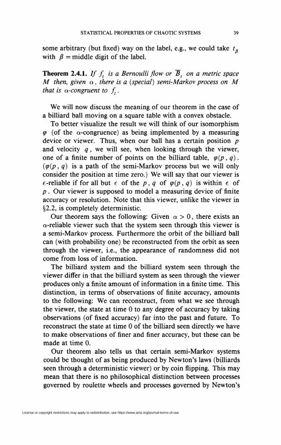
STATISTICAL PROPERTIES OF CHAOTIC SYSTEMS 39
some arbitrary (but fixed) way on the label, e.g., we could take t» with /? = middle digit of the label.
Theorem 2.4.1. If ft is a Bernoulli flow or Tït on a metric space M then, given a, there is a {special) semi-Markov process on M that is a-congruent to ft.
We will now discuss the meaning of our theorem in the case of a billiard ball moving on a square table with a convex obstacle.
To better visualize the result we will think of our isomorphism (p (of the a-congruence) as being implemented by a measuring device or viewer. Thus, when our ball has a certain position p and velocity q, we will see, when looking through the viewer, one of a finite number of points on the billiard table, cp{p, q). {<P(P 9 q) is a path of the semi-Markov process but we will only consider the position at time zero.) We will say that our viewer is e-reliable if for all but e of the p, q of q>(p, q) is within e of p . Our viewer is supposed to model a measuring device of finite accuracy or resolution. Note that this viewer, unlike the viewer in §2.2, is completely deterministic.
Our theorem says the following: Given a > 0, there exists an a-reliable viewer such that the system seen through this viewer is a semi-Markov process. Furthermore the orbit of the billiard ball can (with probability one) be reconstructed from the orbit as seen through the viewer, i.e., the appearance of randomness did not come from loss of information.
The billiard system and the billiard system seen through the viewer differ in that the billiard system as seen through the viewer produces only a finite amount of information in a finite time. This distinction, in terms of observations of finite accuracy, amounts to the following: We can reconstruct, from what we see through the viewer, the state at time 0 to any degree of accuracy by taking observations (of fixed accuracy) far into the past and future. To reconstruct the state at time 0 of the billiard seen directly we have to make observations of finer and finer accuracy, but these can be made at time 0.
Our theorem also tells us that certain semi-Markov systems could be thought of as being produced by Newton's laws (billiards seen through a deterministic viewer) or by coin flipping. This may mean that there is no philosophical distinction between processes governed by roulette wheels and processes governed by Newton's
License or copyright restrictions may apply to redistribution; see https://www.ams.org/journal-terms-of-use
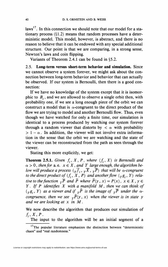
40 D. S. ORNSTEIN AND B. WEISS
laws17. In this connection we should note that our model for a stationary process (§1.2) means that random processes have a deterministic model. This model, however, is abstract, and there is no reason to believe that it can be endowed with any special additional structure. Our point is that we are comparing, in a strong sense, Newton's laws and coin flipping.
Variants of Theorem 2.4.1 can be found in §5.2.
2.5. Long-term versus short-term behavior and simulation. Since we cannot observe a system forever, we might ask about the connection between long-term behavior and behavior that can actually be observed. If our system is Bernoulli, then there is a good connection:
If we have no knowledge of the system except that it is isomorphic to Bt, and we are allowed to observe a single orbit then, with probability one, if we see a long enough piece of the orbit we can construct a model that is a-congruent to the direct product of the flow we are trying to model and another Bernoulli flow. Thus, even though we have watched for only a finite time, our simulation is identical to a process produced by watching our system forever through a random viewer that distorts by < a with probability > 1 - a. In addition, the viewer will not involve extra information in the sense that the orbit we are watching and the state of the viewer can be reconstructed from the path as seen through the viewer.
Stating this more explicitly, we get:
Theorem 2.5.1. Given ft, X, P, where (ft, X) is Bernoulli and a > 0, then for a. e. x e X, and T large enough, the algorithm below will produce a process (Tft, TX, TP) that will be a-congruent to the direct product of( j \ , X, P) and another flow (Tgt, Y) relative to the function TT and P where P(y, x) = P(x), x e X, y e Y. If P identifies X with a manifold M, then we can think of (Tgt, Y) as a viewer and if TP is the image of TP under the a-congruence, then we see TP(y, x) when the viewer is in state y and we are looking at x in M.
We now describe the algorithm that produces our simulation of ft,X,P.
The input to the algorithm will be an initial segment of a
The popular literature emphasizes the distinction between "deterministic chaos" and "real randomness."
License or copyright restrictions may apply to redistribution; see https://www.ams.org/journal-terms-of-use
STATISTICAL PROPERTIES OF CHAOTIC SYSTEMS 41
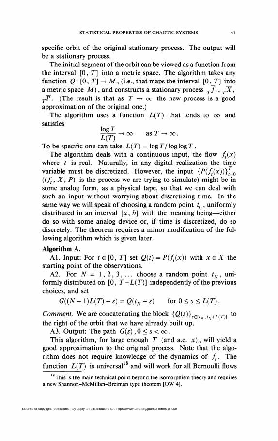
specific orbit of the original stationary process. The output will be a stationary process.
The initial segment of the orbit can be viewed as a function from the interval [0, T] into a metric space. The algorithm takes any function Q: [0, T] —• M, (i.e., that maps the interval [0, T] into a metric space M), and constructs a stationary process Tft, TX, TP. (The result is that as T —• oo the new process is a good approximation of the original one.)
The algorithm uses a function L(T) that tends to oo and satisfies
Z(Tp°° a s 7^°°-To be specific one can take L(T) = log T j log log T.
The algorithm deals with a continuous input, the flow ft(x) where t is real. Naturally, in any digital realization the time variable must be discretized. However, the input {P(ft(x))}f=Q
({ft, X, P) is the process we are trying to simulate) might be in some analog form, as a physical tape, so that we can deal with such an input without worrying about discretizing time. In the same way we will speak of choosing a random point t0, uniformly distributed in an interval [a, b] with the meaning being—either do so with some analog device or, if time is discretized, do so discretely. The theorem requires a minor modification of the following algorithm which is given later.
Algorithm A. Al. Input: For t e [0, T] set Q(t) = P(ft(x)) with j c e l t h e
starting point of the observations. A2. For JV = 1 , 2 , 3 , . . . choose a random point tN, uni
formly distributed on [0, T-L(T)] independently of the previous choices, and set
G((N - l)L(T) + s) = Q(tN + s) for 0 < s < L{T).
Comment We are concatenating the block {Q(s)}se[t t +UT]\ t 0
the right of the orbit that we have already built up. A3. Output: The path G(s), 0 < s < oo. This algorithm, for large enough T (and a.e. x), will yield a
good approximation to the original process. Note that the algorithm does not require knowledge of the dynamics of ft. The function L(T) is universal18 and will work for all Bernoulli flows
18
This is the main technical point beyond the isomorphism theory and requires a new Shannon-McMillan-Breiman type theorem [OW 4].
License or copyright restrictions may apply to redistribution; see https://www.ams.org/journal-terms-of-use
42 D. S. ORNSTEIN AND B. WEISS
in spite of the lack of uniformity of the ergodic theorem. The only problem might come from a bad starting point, but we assume implicitly that the data with which we are presented reflect the physically significant invariant measure. Unfortunately, the algorithm as such fails to give a-congruence since the resulting process may not have sufficient entropy. We can correct for this by artificially adding some fixed entropy. To do this we add intervals of length one between the successive blocks of lengths L(T) that the algorithm is concatenating, and label these intervals independently with a collection of labels of size 2 ( r ) . This will ensure that the resulting process, for T large enough, will have entropy greater than the entropy of the given process (ft, P).
Remark. The result in §2.4 (and the result above) implies that the Bernoulli flows can be modeled by a finite state machine (a computer) equipped with a roulette wheel. We may ask if there is an algorithm that allows us to produce a good simulation if we know the equations of motion.
The usual approach is the following: We discretize time and phase space and approximate the vector
field to determine how one of our discrete points in phase space will move to another discrete point in one unit of time. If we discretize finely enough and approximate the vector field well enough, then we can iterate this procedure and approximate a solution to our equations for a long period of time. However, if we keep iterating, our simulation will eventually be periodic (a computer is a finite state machine) and no periodic orbit can be close most of the time to a generic orbit of Bt or any mixing flow.
If, however, our computer is equipped with a random device that acts like a roulette wheel, then the situation can be remedied in the following seemingly paradoxical way: Iterate our equation L times and then jump in a random way to another point, flip a coin whether to decide to wait 0 or /? units of time {fi/L is irrational, 0 < /? < 1), iterate L times again, etc. If our original system is Bt, and the invariant measure has bounded density with respect to Lebesgue measure, then we can prove that if L is large enough and we have discretized finely enough and approximated well enough (depending only on L), then the computer simulation will be a-congruent to the direct product of the original flow and the Bernoulli flow. This means that the approximation is good for all time and even that the simulated process could have been
License or copyright restrictions may apply to redistribution; see https://www.ams.org/journal-terms-of-use
STATISTICAL PROPERTIES OF CHAOTIC SYSTEMS 43
produced by watching the system through a random viewer that distorts by < a with probability > 1 - a . (In addition, the viewer will not lose information in the sense that the orbit we are watching and the state of the viewer can be reconstructed from the path as seen through the viewer.)
Our random jumps could be taken to be uniform over the whole discretized phase space or uniform over a discretized ball of radius r around our position when we jump. (Our computer simulation can be thought of as a flow if we stay at each discrete point for our discrete unit of time.)
2.6. Instability, or when a-congruence fails.
I. All of our results about a-congruence that we have presented depend on Bernoulliness in an essential way and are for the most part false, in the non-Bernoulli case. Not only are the relevant processes not a-congruent; they even fail to satisfy part of the defining properties of a-congruence in a quantitative way. The reason for this is that any non-Bernoulli process is quantitatively different from all Bernoulli processes. To make this precise we introduce the notion of processes being a-disparate.
Definition of a-disparate. Processes ( ƒ,, X, P), ( ft, X, P) are a-disparate if for almost every x € X, and almost every I G I , the set of V s for which
d(P(ft(x)),P(ft,(x)))>a
has density > a . (d measures the distance between points in the common range of P and P).
The appropriate sets of x and x can be described independently of this definition, as the generic points of the flows ft, ft, respectively. These are the typical points for which time averages convergence to the spatial averages for all continuous functions of the process.
For two fixed processes, the supremum of the a's for which they are a-disparate defines a metric on processes, called the ^-metric. It plays an important role in the isomorphism theory of Bernoulli flows and will be discussed in detail in the next chapter. Here is the basic result:
Theorem 2.6.1. If {ft, X, P) is not Bernoulli and P is a generator, then there is a positive a > 0, such that ( ft, X, P) and any Bernoulli (ft,~X,7) are a-disparate.
License or copyright restrictions may apply to redistribution; see https://www.ams.org/journal-terms-of-use
44 D. S. ORNSTEIN AND B. WEISS
Let's consider the results of §2.2 in this light. There the intrinsic perturbations give rise to Bernoulli flows regardless of the nature of the original flow. (In B we must assume that the process that produces the interference is Bernoulli.) Thus for a non-Bernoulli flow ft, there is an a > 0 such that all those intrinsic perturbations, no matter how small, are a-disparate from ft. In this way microscopic perturbations that are too small to see will have a cumulative macroscopic effect. This effect will be observable in a strong way as we shall see a little later on.
II. In Theorem 1 we see the extent of our being able to model by Bernoulli processes. Suppose, however, that we are interested in modeling with semi-Markov flows or semi-multi-step Markov flows (or in discrete time, Markov or multi-step Markov processes). If a semi-Markov flow or process has no periodic factor then it is Bernoulli and in general it is the direct product of a Bernoulli and a rotation. A system will be a-disparate from this larger class if it is not the direct product of a Bernoulli flow and the inverse limit of rotations (which can be thought of as a clock that gives seconds, minutes, hours, days, ... and so on with an infinite number of nested periods).19 This makes good sense both in discrete time and continuous time.
The class of products of Bernoulli and inverse limits of rotations is stable under factors and ^-limits. This follows from Thou-venofs relative isomorphism theory and FieldsteeFs extension to continuous time.
The next theorem is due to D. Rudolph and G. Schwarz [Rud-Sch] in discrete time and K. Park [Pa] in continuous time.
Theorem 2.6.2. (ft, X, P), P generating, is the d-limit of semi-multi-step Markov flows10 if and only if ft is the direct product of a Bernoulli flow and an inverse limit of rotations.
Thus, if ft is not the direct product of a Bernoulli flow and an inverse limit of rotations then, given a generating partition P, there is an a > 0 such that (ft, P) is a-disparate from any semi-multi-step Markov flow.
The output of a finite state machine equipped with a roulette wheel can be modeled by a semi-multi-step Markov flow (or, in
19 A more formal description is given in §3.7.
20
In a semi- «-step Markov flow we remain at each of a finite number of states si, a fixed length of time ti and then jump with a probability distribution that depends on st and the previous n states.
License or copyright restrictions may apply to redistribution; see https://www.ams.org/journal-terms-of-use
STATISTICAL PROPERTIES OF CHAOTIC SYSTEMS 45
discrete time, a multi-step Markov process) and Theorem 2 tells us exactly which processes can be modeled by the outputs of such machines. In particular the existence of a non-Bernoulli K automorphism means that there is a discrete time process with no deterministic part whose randomness cannot be explained in terms of roulette wheels.
Since most of our results involve modeling or approximating by Bernoulli or semi-Markov processes, they fail in a quantitative way when we stray too far from the Bernoulli case.
III. a-disparate processes are quantitatively different and one might ask whether or not this difference can actually be observed. More generally, if we watch a sample output P(ft(x)) of a process (ft, X, P) andji sample output Q(gt(y)) of (gt,X,Q), can we estimate their d-distance?
If we are allowed to watch forever, then there is no real problem because the Birkhoff ergodic theorem tells us that, with probability one, the entire process ( ft, X, P) can be reconstructed from a sample infinite orbit {P{ft(x))}^l0 (we assume that P generates).
The following theorem captures our idea of observability in a better way.
Theorem 2.6.3. There is a universal algorithm with the following properties:
(a) The input is a pair of functions from the interval (0, T) to a metric space, {Pif^x))}1^, and {Q(ft{x))}^.
(b) The output is a number DT (our estimate of the d-distance). If f(x) is Bernoulli or the direct product of Bernoulli and an inverse limit of rotations, then for almost every x, y chosen according to product measure on X x Y, DT
converges as T —> oo to the d-distance between ( ft, X, P) and {gt,Y,Q).
Remark 1. The above algorithm is robust in the sense that if we change each input by < /? in the Lx sense, then DT change by <2fi. Remark 2. If we make no assumption on ( ft, X, P) or (gt, Y, Ö), then liminfD, will be greater or equal to the d-distance between (ft, X, P) and {gt,Y, Q).
Remark 3. One can prove that there is no algorithm that will work for all {ft,X9P) and (gt,Y,Q).
License or copyright restrictions may apply to redistribution; see https://www.ams.org/journal-terms-of-use
46 D. S. ORNSTEIN AND B. WEISS
2.7. Further directions for a-congruence. When do we have statistical stability? Structural stability is limited to axiom A and few realistic systems are axiom A. We also ask when is there a canonical measure like the SBR measure, and when do we get stability results for the measure of maximal entropy?
Theorem 2 (see 1.2) shows that we can go beyond axiom A for certain perturbations. Another example due to Eloranta [E] is the following. Perturb the billiard system by taking two copies of a billiard table very close together and cutting a hole where each obstacle is, and connecting the opposite holes with a smooth surface (of negative curvature). The billiard system is then approximated by a geodesic flow and the approximating flow is a-congruent to the billiard system, after a small rescaling of time, (a —• 0 as the tables get closer.) This example is interesting for two reasons. ( 1 ) The conclusion of structural stability cannot apply because a.e. orbit will spend a small amount of time circling the hole, (2) The perturbation, although small, gives a qualitatively different system. Thus billiards can be smoothed without changing the long-term dynamics.
If we restrict the kind of perturbation enough, we can get stability results for wide classes of systems. For example, if (ft, M) is a smooth Bernoulli flow on a compact three-dimensional manifold M preserving a measure absolutely continuous with respect to Rie-mannian volume, and if we perturb ft by changing the speed by a small C2 function (which may vary from point to point along an orbit) then (ft, M) will be a-congruent either to the perturbed flow ft or to ft times a rotation (this is the analog of Theorem 2.1.4). The question now is when can the alternative be ruled out?
We can also ask for systems other than axiom A that are stable under random perturbations. It seems that this is where the gap between what we can prove and what is true is the greatest. Most reasonable random perturbations are Bernoulli. If our original system is not Bernoulli we have no possibility of stability (see §2.6) so we assume that our original system is Bernoulli. Therefore, what we need to understand is how the invariant measure and the entropy change under the perturbation? For example, we do not know if there is a Bernoulli diffeomorphism of a two-dimensional manifold that is not stable under the perturbation of Theorem 2.2.1 when we jump with uniform distribution in a disk of small radius around the point we land at under the diffeomorphism.
License or copyright restrictions may apply to redistribution; see https://www.ams.org/journal-terms-of-use
STATISTICAL PROPERTIES OF CHAOTIC SYSTEMS 47
We can also look for different kinds of random perturbations. One example is the following: Take an ergodic automorphism of T, of a compact Abelian group &. Perturb the T process by taking any stationary process with values in 9, concentrated near 0, and adding this process to the T process. We have stability when the noise process is Bernoulli.
Any time we have a stationary process and another process that is supposed to approximate it, we can ask if the approximation is good for arbitrarily long time intervals. In this spirit, we can ask if the processes are close in the d sense or the sense of a-congruence. (For example, Brownian motion confined to a finite interval with reflecting barriers is often approximated by a random walk.) Eloranta has results along these lines that extend the Donsker invariance principle [E].
We can also study a-congruence for other systems like infinite particle systems. Here the group is Z " x R . (Zn corresponds to translation of a «-dimensional lattice and R to the time evolution.) In certain cases Steif [Ste] has shown that the system is a-congruent to a system where the lattice is made up of an infinite number of large disjoint cubes that do not interact with one another. Steif s cases are: (1) The M < e condition [Lig] where there is only one invariant measure. (2) The two extreme measures for monotone systems—each lattice site wants to imitate its neighbors (see [Lig]). These systems include most of the systems studied. This result is interesting because infinite particle systems are supposed to model large finite systems, and this result says that they do in a very strong sense.
We can also ask for a-congruences that preserve some additional structure. One example is the (n - l)-frame flow on an «-dimensional manifold of negative curvature, n odd, n ^ 7 . In this case, we have a group larger than R acting. (We can rotate the frame at a point.) Using the isomorphism theory for this more general group, one can show (using results of Brin and Gromov [BrG]) that if we perturb the metric, the new frame flow will be a-congruent (after a small rescaling of time) to the original one and the conjugating map will take the collection of frames at a point to the collection of frames at another point.
Understanding particular systems has been an ongoing project. Here is a recent example where work still needs to be done: Wo-jtkowski [Wo 1, Wo 2] has shown that the following system has
License or copyright restrictions may apply to redistribution; see https://www.ams.org/journal-terms-of-use
48 D. S. ORNSTEIN AND B. WEISS
FIGURE 2
positive entropy: a ball of nonzero mass acted on by gravity and bouncing in an elastic way (no energy loss) where the floor is shaped like a wedge and n/2 < 6 < n (Figure 2).
The Katok-Strelcyn [KatoStr] modification of Pesin theory almost certainly takes care of the singularities and if so, the system is either Bt or 2?, on each ergodic component. In either case the system would be a-congruent to a semi-Markov process as in §2.4. We could ask if a small change in 6 produces an a-congruent system where we can make a arbitrarily small by making the change in 6 sufficiently small. (When 6 — n/2 or 6 = n the system has zero entropy and will therefore change discontinuously). The force of gravity could be taken as constant or inversely nonpro-portional to the distance to the center of the earth. Will the latter small perturbation produce an a-congruent system with small a ? Some of the interest in the above system lies in the fact that it is so close to a ball bouncing on a flat floor—the first system one studies in calculus.
3. A SURVEY OF SOME ABSTRACT ERGODIC THEORY21
3.1. The ^-distance. When a stochastic process xn is observed through a noisy medium, the observed process can be represented
21 The results in this section that are not specifically referenced can be found in
[OW l ] o r [ 0 1]. A stochastic process {x^™^ is a collection of random variables defined on
some probability space (Q, I , ju) with values in some set A . The measure on A defined by the image of /z under the mapping œ «-• {x^œ)}0^^ is called the distribution of the process or the joint distribution of the variables {xn} . The process is called stationary if for each p , the distribution of {xn+p}
<^L_00 is the same as that of {x^™^ . If the process is stationary, then the shift T on Az
(xn{co) = xn_l{Tco)) preserves JU and we can therefore also model a stationary process by a measure-preserving transformation T acting on a space X = A and a function P on X (P(co) = x0(co)). Note that V ^ r ' P generates the entire a -algebra of X (up to sets of measure 0). We denote this setup by (T, X, P), or if we want to emphasize the measure by (T, fx, P), etc.
License or copyright restrictions may apply to redistribution; see https://www.ams.org/journal-terms-of-use
STATISTICAL PROPERTIES OF CHAOTIC SYSTEMS 49
by Xn = Xn + en >
where the ert represent the error process. If the medium is not very noisy, then en will be small most of the time and then for most time instants n, xn will be close to xn . This is the archetypal example of two processes that we wish to think of as being close to one another. The ^-distance is a formal way of measuring the distance between processes that takes into account not merely the finite distributions but also the long-range behavior in the same way that the xn and the xn processes above are close. Since discrete time stochastic processes are simpler than continuous time ones, we will begin by explaining the ^-distance in that case, and further suppose that the processes are finite valued.
When one is presented with two distinct stochastic processes {xn} and {yn}, then it makes no sense to ask questions such as what is the probability that xQ = y1, since these random variables need not be defined on the same probability space. Any way of defining the two processes on the same space is called a joining of the two processes. More formally a joining is a stochastic process of pairs [xn, yn} such that {xn} has the same distribution, or probability laws as {xn} and {yn} has the same distribution as {yn} . There is always at least one joining of any two given processes—the independent joining—obtained by declaring that the xn variables are all independent of the yn variables. We shall be dealing with stationary processes and in that case by a joining we shall mean a stationary one, i.e., {(xn , Fw)}!foo *s a^s0
a stationary process. There are cases where the independent joining is the only joining; however, in the situation that we will be studying there are typically many different joinings.
Given two processes {xn}, {yn} we seek a joining between them {(xn , yn)} so that
(*) P r { * 0 ^ o } shall be as small as possible. The infimum of (*) as we range over all possible joinings is the rf-distance between {xn} and {yn}. Formally _
d({xn}, {yn}) = inf Pr{x0 ^ y0},
where {(xn,yn)} ranges over all joinings of the given processes. This metric is much more stringent than the metric defined by the finite distributions. Here is a simple example to keep in mind.
License or copyright restrictions may apply to redistribution; see https://www.ams.org/journal-terms-of-use
50 D. S. ORNSTEIN AND B. WEISS
Consider the two state Markov chain defined by the transition matrix
( l - e e J and stationary measure (j, \). When e = 0, this is a pure periodic process with precisely two output sequences. As long as e > 0, the d-distance between this process and the pure periodic is \ , corresponding to the independent joining (indeed there is no other one). To see the former, observe that by stationarity
Pr{*0^70} = i £ > { * , . # 7,.}.
Now for a typical xt output when e is very small we will see long strings of alternations between the two states. However these will be out of phase about half the time with respect to either of the purely periodic alternations represented by {y •} . In finite distributions, of course, this family of Markov chains is continuous all the way down to 6 = 0 . The family is continuous in the d-distance for e > 0. While fairly elementary, this fact is nontrivial; see §3.5.
To compute the ^/-distance between two processes in terms of the finite distributions, one proceeds as follows. Define the d-distance between {xn}^l9 {yn}„={ by
- 1 N
(**) d({xn}N
n=x, {yH}^i) = u-inf- u M E P r ^ * 7n) >
where the infimum is over all joinings (now not required to be stationary) between the xn's and the yn's. It is a fact that
Our main interest in this metric is the behavior at zero, and so variant definitions which give that same behavior are sometimes more useful. For example, the right-hand side of (**) can be replaced by
inf {e : for some joining (xn ,yn),
Pr{~\{l<n<N:xn^yn}\>e}<ey
With this variant it is easy to see what to do if the process is not finite valued but takes values in a fixed compact metric space
License or copyright restrictions may apply to redistribution; see https://www.ams.org/journal-terms-of-use
STATISTICAL PROPERTIES OF CHAOTIC SYSTEMS 51
(M, d). We take then the infimum of all e > 0 for which there is some joining such that
f i N
y„)>e\<e.
After this discussion of the more standard situation we come to the one we need here. Now we have to begin with a measure-preserving flow ft on a measure space (X, âS, fi). For example ft could be a smooth flow on a manifold X with SB the Borel sets and // a fixed invariant measure. A process will be defined by such a flow and a mapping
which is a measurable mapping from X to a compact metric space (M, of). We will sometimes refer to P as a partition of X. For example, if X is a compact manifold, then the identity map with M = X defines a process. To any point x e X, and any T > 0, we associate a path in M defined by
PT(x) = {P(ft(x)):0<t<T}
and call that the P-T name of x . This map takes the measure /u onto a probability measure on M[ 'T ] , the space of [0, T]-paths in M, which we denote by juT . These are the finite distributions of the process P. Had we been considering a finite space M, and a discrete time flow {fn) , then these would just be our earlier finite distributions. For two measures juT, vT on M[ ' r ] define
d(juT, vT) = inf{/?},
where /? ranges over all positive numbers for which there is some measure X on M[0 'T] x M[0 ' r ] satisfying
(1) 7Tj o A = / / r , n2o X = uT; where 7rx 2 are the coordinate projections. This is a formal way of saying that A is a joining of fiT and vT.
(2) xl(u,v):j^Td(u(t),v(t))>À<fi,
Here u(t) and v(f) denote a [0, T]-path or an element in M[0, T] i.e., u(t) = P(ft(x)) for some x.
If vT represents the finite distribution of some process (gt >
v > Ö) with values in M then we define
d((ft,fi,P),(gt,i',Q))= lim rf(/ir, vT). i — • O O
License or copyright restrictions may apply to redistribution; see https://www.ams.org/journal-terms-of-use
52 D. S. ORNSTEIN AND B. WEISS
For the whole process this guarantees that for any /? greater than this of-distance there is a joining between them, a measure X on {M x M ) R , so that
JL{(u,v):d(u(0),v(0))>fi}<fi.
The notion of the ^-distance is implicit in the concept of a-congruence. Indeed two processes that are a-congruent are within a in the ^-metric, but a-congruence involves much more since the (close) joining of the processes is required to be an isomorphism between them. 3
d is not very useful for studying deterministic processes like the linear flows on the torus. Here almost any two different flows are far apart in d. Indeed, defining
for (x,y) e T2 , if (a, b) and (c, d) are not rationally related then one can show that the only joining possible between processes defined by ft and gt are independent joinings. It is precisely for chaotic systems, the ones that have positive entropy, and are very far from such deterministic systems, that the df-metric proves to be a very useful tool.
3.2. Entropy and a-entropy. For a continuous mapping T of a compact metric space (M, d) the topological entropy is defined by
limlimsup — log{minimal number of (N, e) balls e-*0 W - K » iV
that cover the space M},
where the (N, e) ball means a set B that satisfies
d(Tnx, Tny)<e, all 0 < n<N, allx,yeB.
This quantity measures the exponential growth rate of the number of diverging orbits and is denoted by
The topological entropy is zero for nice flows like the irrational flow on the torus, and its positivity is an indication of some kind
23
Rudolph has unpublished examples that show that it is possible for processes to be close in the d sense and isomorphic without being close in the sense of a-congruence. In these examples there are joinings that are isomorphisms and joinings that produce a good c/-match but no joining that does both.
License or copyright restrictions may apply to redistribution; see https://www.ams.org/journal-terms-of-use
STATISTICAL PROPERTIES OF CHAOTIC SYSTEMS 53
of chaotic behavior or sensitive dependence on initial data. In the presence of a measure fi that is T-invariant it is natural to count the minimum number of (TV, e) balls required to cover a set in X of large measure rather than all of X. For ergodic measures it turns out that fixing any c> 0 and calculating
lim lim sup — log{minimal number of (N, e) balls
neededto fill a set of //-measure c in X)
gives the same number independently of c, and this number is called the measure-theoretic entropy of the system (M, T, / / ) , denoted by
For flows ft, the measure-theoretic entropy was originally defined by means of the discrete time skeleta fnd . It was J. Feldman who showed how to define the entropy of a flow, with respect to a finite partition, directly in terms of the flow [Fe 2]. His definition is close in spirit to the one we just gave and works just as well for compact partitions. For a measurable flow (X, 3S, ju, ft) and a partition P : X —• M, a compact metric space, define a P — a — T ball to be a set B c X that satisfies
j J d{P{ftx), P(fty)) dt<a all x, y G B.
Now define for 0 < c < 1
= lim sup -= log{minimal number of (P, a, T) balls
needed to fill a set of // measure c in X}.
For ergodic processes one shows that this limit is independent of c G (0, 1) and we call that limit the a-entropy of the process, denoted by h(P, a ) . The entropy of the process (P, /J) is defined by
h(P, ft) = lim h(P, a)
and finally the entropy of the flow is defined to be
h(ft) = sup(P,ft), p l
where the supremum ranges over all compact partitions, or over all finite partitions. This turns out to be the same as the more usual definition which is h(f{).
License or copyright restrictions may apply to redistribution; see https://www.ams.org/journal-terms-of-use
54 D. S. ORNSTEIN AND B. WEISS
We have the formula first proved by Abramov, h{ ft ) — \t0\h(ft). Note that h(ft) refers to the entropy of the flow while h(ft ) , where t0 is thought of as a fixed real number, is the entropy of the transformation ƒ, .
It is trivial that under rescaling, ft = fct, we have
h(7t,P,a) = \c\h{ft,P9a),
and thus also in the limit as a —• 0
h{P9ft) = \c\h(P,ft).
When P is changed to a P that is close to P in the sense that for some small ô > 0
(*) /i(x: d(P(x), P(x)) <S)>1-S,
then for most of the space X, (P, a, T) balls are (P, (a + 2<J), T) balls so that for ergodic processes
h(P, a + AS) < h(P, a) < h(P, a - 43).
In the limit, as a —• 0 this continuity in P is lost and in general it is not true that as P„ —• P in the metric defined by (*) above,
h{ft,P„)-+h{ft,P).
In the totally discrete situation, when the number of elements in the partition is finite and held fixed and the time discretized, the entropy depends continuously on the partition. This continuity allows for some results to be formulated more simply in that situation, and it is the lack of continuity in our setting that is responsible for the cumbersome definition of "finitely determined processes" below.
One can establish a version of the Shannon-McMillan theorem for the a-entropy and it plays a key role in the proofs of the theorems in the rest of this chapter. The remarkable thing is that a real meaning is given thereby not only to the process entropy h(P, ft) but to the a-entropy for each value of a. Here is one version of the theorem:
Given e > 0, if T is sufficiently large then there is a subset X0 c X satisfying
1. fi(X0)>l-e; 2. for any P-a-T ball B c X0
ju(B)<exv{-T(h(P,a)-e)};
License or copyright restrictions may apply to redistribution; see https://www.ams.org/journal-terms-of-use
STATISTICAL PROPERTIES OF CHAOTIC SYSTEMS 55
3. there is a covering of X0 by fewer than
exp{T(h(P,a) + e)}
(P,a,T) balls.
Another way of understanding (3) is to observe that, in the presence of (2), (3) implies that most of the (P9 a , T) balls in that covering collection have measures which lie in the
cxp{-T(h(P,a)±e)}.
In the discrete situation one can take a = 0 and then there are canonical (P, N) balls which are simply the atoms of the partitions vf "n1 f~lP. Thus the classical Shannon-McMillan theorem simply asserts that most atoms of V ^ 1 f ~ l P have exponential size approximately equal to exp{-Nh(f{P)} . In general the formulation is of necessity more complicated.
The Shannon-McMillan theorem has a simpler statement for very small a. This statement is about centered (P, a, T) balls. We define a (P, a, T) ball centered around y(t) e M[0,T] to be the set of y such that
j;J*d{P{fty)9y{t))dt<a.
If we use centered (P, a, T) balls, the value of a-entropy will change but the above Shannon-McMillan theorem will still hold and we will get the same limit h(P, ft) as a -• 0. In terms of centered balls we get a Shannon-McMillan theorem for h(P, ft)\
Given e > 0, if a is small enough and T large enough (given a), then there is a subset XQc X, ti(XQ) > 1 - e and any (P9a, T) ball with center in X0 has measure between exp{-T[h(P, ft)±e]} and there is a covering X0 by fewer than exp{T[h(P, ft) + e]} (P,a,T) balls.
The way in which a-entropy was defined makes it clear that the topological entropy of the flow gives an upper bound for the measure theoretic entropy (for this and the following result see the discussion in Szlenk's book [Sz]). The fact that there always exists invariant measures which approach the topological entropy lies a little deeper and requires the construction of invariant measures.
With the concept of entropy at our disposal we can return to our earlier discussion of predictable and nonpredictable processes. The results are easier to state in discrete time (for continuous time flows
License or copyright restrictions may apply to redistribution; see https://www.ams.org/journal-terms-of-use
56 D. S. ORNSTEIN AND B. WEISS
ft, these results are best formulated by considering the discrete samplings of the flow {ft n}nez) . A finite state process {x^™^ is said to be predictable if x0 is a measurable function of the past {xn : n < - 1} . The fundamental connection with entropy is the following: A finite state process {x^™^ is predictable if and only if it has zero entropy, A flow has zero entropy if and only if the discrete samplings of any measurable function are predictable.
Sometimes deterministic is used instead of predictable. Standard approximation theorems yield that if we are satisfied with predicting x0 up to a small error then & finite number of observations in the past suffice. Examples of such systems include periodic systems such as the simple pendulum or quasi-periodic systems like billiards on a rectangular table with no obstacles. Geometric examples include the horocycle flow on a negatively curved manifold or the geodesic flow on an ellipsoid.
At the other extreme are the systems that are completely nonpre-dictable, where no nonconstant measurement on the system taken at discrete times (i.e., ntQ) is predictable. These are exactly the systems that have no factors of zero entropy. These systems are also called A'-systems and for obvious reasons systems with completely positive entropy.
By a theorem due to Pinsker, Rohlin and Sinai [RoSi] these systems also have the following characterization: A process {xn}nEZ is completely nonpredictable if and only if, for any k, and e > 0, there is an N so that the distribution of {xx, x2, . . . , xk} conditioned on {xn: n < -N} is within e of the unconditioned distribution but for a set of measure < e of specific outcomes of {xn : n < -N}. Informally, any fixed number of observations {x{, . . . , xk) is approximately independent of the remote past (and remote future). A flow is K if and only if any measurement taken at discrete times is completely nonpredictable.
Examples here are all the examples of Bernoulli flows that we have already discussed, but in addition there are non-Bernoulli examples, [O 7]. The first smooth example was given by Katok [Ka 1], and some rather natural smooth ones are discussed in Rudolph [Rud 7].
3.3. Extremal processes. We start by recalling the definition of Bernoulli shifts as those transformations that arise from independent processes. ft is a Bernoulli flow if ft is a Bernoulli shift for some fn. There are various characterizations of Bernoulli
License or copyright restrictions may apply to redistribution; see https://www.ams.org/journal-terms-of-use
STATISTICAL PROPERTIES OF CHAOTIC SYSTEMS 57
processes. The last one to be discovered was the property of extremality due originally to J.-P. Thouvenot and first used extensively by D. Rudolph in his work on extensions of Bernoulli shifts. Since this characterization works for infinite entropy flows as well as finite entropy discrete time actions, we describe it first. To begin with the simplest situation, consider a discrete process {xn} with values in the finite set A. We say that the process is extremal if the measure jun that it defines on «-names (i.e., An) cannot be divided up into a small number of pieces that are far away from nn in the d-metric. In formal terms we require that for any e > 0, there is some ô > 0 and Ne, and for all n > Ne
if jun , the measure 4 on An defined by {xt} is decomposed as a convex combination
i=\
of probability measures kt, then most (measured by ct) of the kt
satisfy
(*) d(/in , kt) < e .
In more precise terms
T,ci>l~€
iei where I consists of all those indices that satisfy (*).
The basic fact is that independent processes are extremal in the sense just described. It is easiest to prove this fact using the notion of finitely determined (see §3.5 below). For flows and compact partitions one can use the very same definition for extremality:
Definition. A process (ft, P) is extremal if given e > 0 there is some ô > 0 and T0, and for all T > T0 if /uT denotes the measure on P - T names and
i=i
is a convex decomposition of /uT into probability measures jut, then
E c / > 1 " " c
iei Here is how the stochastic process {xt} defines the measure
License or copyright restrictions may apply to redistribution; see https://www.ams.org/journal-terms-of-use
58 D. S. ORNSTEIN AND B. WEISS
where iel if d(/it, fiT) < e .
Recall that a process P is called a generator for the flow (X, 32, /u, ft) if the cr-algebra generated by P , V ^ / J P coincides with c^ modulo yU-null sets.
Theorem 3.3.1, If one generator o f a flow is extremal so are all processes defined by that flow, and the flow is Bernoulli {isomorphic to Bct for some constant c > 0, or to Bf°).
If in our definition of extremal we restricted the convex combinations of measures ut to be those that come from partitioning X, we would get an equivalent definition.
Extremality in the latter form is especially easy to interpret in terms of predictability. Suppose ft is a Bernoulli flow on a metric space M, and that we would like to predict, to within e , the T-name (M - T-name) of a point (in M) that we can see with only finite precision. The finite precision device, through which we view our starting point, partitions M into a finite number of pieces and extremality says that if there are fewer than 2 T pieces, then with probability 1 - e we can say nothing about T-names if we ignore an average error less than e . Thus exponentially (in T) good precision tells us nothing about the T future if the exponential rate is too slow. This means that if it takes ô~l units of time to get one extra bit of information about the starting point and if ô~l is too large, then no prediction is possible.
Note that the entropy gives the slowest rate for which it is possible to predict arbitrarily well.
3.4. Very weak Bernoulli (VWB). For an independent process the distribution of {x{, ... , xn} conditioned on any past event A of the form
A = {co:xi(œ)=Çi,i<0}
is the same as the unconditioned distribution. You come to the definition of a very weak Bernoulli process by relaxing a little bit on this both in the set of 4's and on the relationship of the unconditioned to the conditioned distribution. We are considering here finite-valued discrete times processes P and use the notation fiN for the measure on iV-names defined by the distribution of
S~1PvS~Vv---vS~ iV/\
License or copyright restrictions may apply to redistribution; see https://www.ams.org/journal-terms-of-use
STATISTICAL PROPERTIES OF CHAOTIC SYSTEMS 59
We have switched to the notation of a measure space (X, £%, / / ) , a measure-preserving transformation S: X -+ X and a finite valued partition P of I . The process (S, P) is said to be very weak Bernoulli (VWB) if, given e > 0, there exists NQ and for all N > NQ and all L the set of all atoms A of V°_LS~lP for which
d{/N\A9ju^)<e
has total measure greater than 1 - e . Here we are using [iPN\A to
denote the measure on P - A/-names obtained by conditioning on the atom A.
The following basic result from the isomorphism theory of Bernoulli shifts provides a way that specific flows can be shown to be Bernoulli since this property is often verifiable [OW 3].
Theorem 3.4.1. (a) The process (S, P), P finite, is very weak Bernoulli (VWB) if and only if
(x, V s ~ n p , n , s \
is a Bernoulli transformation. (b) If for some t0, and finite partitions Pt, P. { refines Pt,
and together they generate under ft {i.e., U;(v!°oo/r"^) ^ ^e
whole a-algebra) and (ft , P.) is VWB then ft is isomorphic to Bct for some c > 0, or B°°. Conversely if ft is isomorphic to Bct, c > 0, or B°° then for any fixed finite partition P, and any t0^0, (ftQ,P) is VWB.
Here is a variant of this property where both L and fi are given infinite values. For C in a set of atoms of V0_ooT~nP that has full measure
( oo oo \
\jT~nP\C,\jT~nP\ = 0 . Note that since the first distribution is not stationary, this doesn't imply that the processes are the same. The rf-distance in (*) should be interpreted as: for some joining between the conditional variables {x^}™ and {xn}™ we have
1 N
License or copyright restrictions may apply to redistribution; see https://www.ams.org/journal-terms-of-use
60 D. S. ORNSTEIN AND B. WEISS
This property may be compared with one of the characterizations of K processes that we gave in §3.2. Instead of saying there that {xx, . . . , xn} becomes independent of the remote past {xn : n < -N} , we could equally well say that a fixed time range {xn : N < n < N + k} in the distant future becomes independent of the past {xn : n < -1} . On the other hand, for VWB processes the past gives vanishingly little information (on average) of the long-term future.
In terms of how knowledge of the past allows us to predict the future we get the following table (observations with finite precision at discrete time intervals).
Class of flow
0 entropy Positive entropy K
Bernoulli
Knowledge of past for a generating observation tells us
Everything about the future Not everything about the future Arbitrarily little about fixed time in dis
tant future Vanishingly little about long-term future
3.5. Finitely determined processes (FD). One of the key concepts that emerged from the proof of the isomorphism theorem for Bernoulli processes is that of processes whose long-range behavior is fixed or determined in the ^-metric by their finite distribution and entropy. Thus, after fixing the short-range behavior (i.e., the distribution of some finite number of variables), the long-range behavior (i.e., the joint distribution of all the variables of the process) is essentially described by a single real parameter—the entropy. The concept makes sense only for finite entropy processes and flows and we restrict to that case throughout this section.
We begin with a definition for finite-valued processes or partitions in discrete time.
Definition. A process (S, P) is finitely determined if given e > 0 there is a ô > 0 and an N such that whenever (S, T) satisfies: close in finite distribution
^distribution (VQ&P) , distribution (WQS~17)} < Ö
License or copyright restrictions may apply to redistribution; see https://www.ams.org/journal-terms-of-use
STATISTICAL PROPERTIES OF CHAOTIC SYSTEMS 61
and close in entropy
\h(S,P)-h(S,P)\<ô
then d((S,P),(S,P))<e.
Since for fixed N the space of distributions on VQS~1P is finite dimensional the specific metric d that is used is not important, one can, for example, use the /^norm between the probability vectors, or the d-metric. The basic observation is that independent processes are finitely determined. That is fairly easy to see using the fact that the only way for the entropy of a process to be close to its theoretical maximum (the entropy of the partition P itself) is for P to be nearly independent of vZl
NS~~lP • After this basic observation is made, one can go on to show that the FD property is preserved under factor maps and this gives some insight into how the concept is very useful.
When working with flows or compact partitions it is best to use the a-entropy even though this definition of finitely determined becomes more cumbersome. This was given by Feldman.
Definition. A process (ft, P) is finitely determined if given e > 0 there is an y > 0 and functions T(fi), S(fi) (that depend both on y and the process) such that if (ft, P) is any process that satisfies for some_/?
(i) hfft,P9fi)>h{ft,Pl-j, (ii) d( distribution v J w / r P , distribution V%lfi)ftP) < S(fi)9
then _ *((ƒ,, 7 ) , (ƒ , , />))<€.
The extra p is necessary since the closeness in distribution required in (ii) depends upon the level /? at which the test process has enough entropy. For T(fi) chosen well (i) and (ii) together will imply
\h(?t979fi)-h{ft,P)\<y since one can easily give upper bounds for the entropy in terms of finite distributions.
The above form of the definition is the one that is used in proving the main isomorphism theorems (the original proof involved a messy discretization of time). However, in applications it is convenient to have another version of the definition in which ordinary entropy rather than a-entropy appears.
License or copyright restrictions may apply to redistribution; see https://www.ams.org/journal-terms-of-use
62 D. S. ORNSTEIN AND B. WEISS
Lemma 3.5.1. If (ft9 P) is finitely determined and P is a finite partition, then given e > 0, there is an y > 0, ô > 0, and T such that if (ft, P) is ergodic and satisfies
(a) ^h(ftQ, 7) > A(y;, P) _ y / o r *om6> t0 e (± , 2) ,
(b) rf(distvj/^, distvJ/,/>) < ? ,
(*) d((ft,P)Aft,P))<£-
Note that h(ft , P) rç/ers to Ae entropy of the Z-action generated
by ft , while h(ft, P) refers to the entropy of the R-action, ft, teR°.
Here is the main theorem concerning FD and Bernoulli processes.
Theorem 3.5.1. (Bt, P) is FD for all P. If (ft, P) is FD for a generator P, then ft is isomorphic to Bct for some constant c.
If S is Bernoulli (S, P) is FD for all P. If (S, P) is FD for a generator P then S is Bernoulli.
In particular if a process is not Bernoulli then we can find finite approximations to it that remain a fixed distance away in d. A zero entropy process (S, P) cannot be finitely determined since the «-step Markov approximation (with a tiny bit of pure randomness thrown in) (Sn , Pn) are certainly close in finite distribution and in entropy but there is no nontrivial (nonindependent) matching between {S 9 P) and (Sn,^n) so that the ^-distance between them is bounded away from zero. Let us take a closer look at rotations of the circle. Any two rotations, Ra, Rp , are fixed distance apart in d no matter what partition we take. Thus in any neighborhood of Ra in the topology of finite distributions (entropy is not an issue since they all have zero entropy) there are an uncountable number of processes, all of whose mutual distance in d are greater than some fixed ô > 0. This is another example of how our results are limited to chaotic systems.
An immediate consequence of the FD property for Bernoulli flows is the following result which has no analogue in discrete time:
Proposition 3.5.1. If ft is a Bernoulli flow and P is a fixed partition, then the mapping
c~(fct,P)
is continuous in the d-metric.
License or copyright restrictions may apply to redistribution; see https://www.ams.org/journal-terms-of-use
STATISTICAL PROPERTIES OF CHAOTIC SYSTEMS 63
For non-Bernoulli flows this kind of continuity can fail dramatically. For the simplest examples consider the Kronecker flows on a torus of any dimension (including 1).
Remark. A result that is much stronger than Proposition 1 was given in §2.3.
3.6. Isomorphism theorems. We begin by stating again the ba-sic definitions. Two measure-preserving flows (X, 38, fi, ft), (X, 38, /Z, ft) are isomorphic if there is a measurable invertible mapping 0: X -+ ~X such that ju(d~l(B)) = Jl(B) for all B G I and
ftoe = doft
for all t. A partition P : X —> M is said to be a generator if the smallest
sub- cr-algebra of 38 with respect to which all ft o P's are measurable is all of 38 (modulo //-null sets). In general this sub-cr-algebra is denoted by P*™, thus P is a generator means that 38 = P*™. While the existence of finite generators for transformations of finite entropy was a nontrivial achievement (first accomplished by W. Krieger [Kri]) it is easy to find compact generators. Indeed if X itself is compact, as is often the case, then P = identity is trivially a generator.
Abstract processes (ft, P), (ft, P) are isomorphic if the flows
(X, P+™ , ft), (X, P+_Z , ft) are isomorphic. Finally, let us repeat again the definitions of y-congruence. First
of all two flows ft, ft defined on the same space M, are y-congruent if they are isomorphic via a mapping 6: M —• M that satisfies
//{x: rf(x, 0(x)) >y} < y ,
where d is a fixed metric on M. Thus y-congruence strengthens the notion of isomorphism by requiring that the correspondence giving the isomorphism be close to the identity in a strong geometric sense.
To compare flows on different spaces from this point of view we need to fix partitions on these spaces with values in the same space (M, d). So flows
(ft,X,P), (ft,X,P)
25We will denote a flow simply by ft or by (X, ft), or by (X, 38 , ft).
License or copyright restrictions may apply to redistribution; see https://www.ams.org/journal-terms-of-use
64 D. S. ORNSTEIN AND B. WEISS
with both P and P taking values in (M, d) are y-congruent relative to P and P if there is an isomorphism
6:X^X
between (ft, X) and (ft, ~X) such that
ti{x:d(P(x),P(6(x)))>y}<y.
Note that this notion depends on more than the abstract process (ft, P) since we require that 0 be an isomorphism even if P is not a generator.
The first definition is a special case of the second when we take & = p = identity. Notice that if (ft,X, P) and (ft,X,P) are y-congruent for small y, then the processes (ft, X, P) and (ft, X, P) are close in of since the map 0 defines a joining between (ft, P) and (ƒ,, P ) . This joining is simply the fi measure lifted up to the graph {(x, 6(x)): x e X} in X x X, The fact that this measure projects onto /7 in the second coordinate is the fact that 6 o fi = Ji,
When processes ( / , , P + ~ , P ) and ( ƒ , , ? ! £ , P) are 0-congruent we will simply call them congruent. In the language of probability theory, congruent processes are identically distributed processes, We_make the following convention: When we write (ft, P) and (ft, P) are congruent or identically distributed, we will always refer to the process (ft, P ^ , P ) . y-congruence, however, refers to the entire cr-algebra, not just the one generated by P . We will also write d(P, P) < y as an abbreviation for fi{x:d(P(x),P(x))>y}<y.
Recall that ft is defined to be a Bernoulli flow (of finite or infinite entropy) if and only if ft is a Bernoulli shift for some fixed t0, A Bernoulli shift is defined as follows. Let Y be a measure space of total measure one. Let Y., -oo < / < oo, be copies of Y, Let X = n!°oo Yt with product measure (points in X are sequences with values in Y). The Bernoulli shift acts by shifting each of the above sequences.
Here is the weak isomorphism (or imbedding) theorem for Bernoulli flows:
Theorem 3.6.1. Let (X, ft) be a Bernoulli flow and P any partition defined on X. (a) Imbedding. If h(ft) > h(ft, P) then there is a partition P on H such that the processes (ft, P) and (ft, P) are identically distributed.
License or copyright restrictions may apply to redistribution; see https://www.ams.org/journal-terms-of-use
STATISTICAL PROPERTIES OF CHAOTIC SYSTEMS 65
(b) Stability of imbedding. If h(ft) > h(ft, P) and there is a partition P on X satisfying
d((?t,?),{ft,P))<a
then for any e > 0 there is a partition P such that
d(P,P) <a + c
and (ft, P) and (ft, P) are identically distributed.
The result in (b) of course is a strengthening of (a), which follows from (b) by beginning with any partition. It is also the more basic result since it gives a hint as to how the theorem is proved. What it shows is that any approximate imbedding, one which is not too distant from the goal, can be changed slightly so as to become an exact imbedding. In all of the subsequent generalizations the same pattern persists—first one establishes an embedding theorem of the type that we just gave and then when both flows are Bernoulli and the entropies are equal one obtains isomorphisms. In the next theorem, part (a) is the basic isomorphism theorem for Bernoulli flows of equal entropy and it appeared first for finite entropy in [O 6]. Part (c) is a refinement which is often useful and says that isomorphisms are prevalent. Parts (b) and (d) deal with ^-congruences and are new; we shall give their proofs in §5.
Theorem 3.6.2. (a) Isomorphism theorem for flows. If (X, ft) and (X, ft) are Bernoulli flows of equal entropy, then they are isomorphic. (b) If (X, ft) and (X, ft) are Bernoulli flows of equal entropy and P, P are partitions that satisfy
d((ft,P),(ft,P))<jQ,
then (X, ft, P) is y-congruent to (X, ft, P). (c) Prevalence of isomorphisms. If (X, ft) is a Bernoulli flow and R is a full entropy partition (i.e., h(ft, R) = h(ft)), then for any ô > 0 there is some R satisfying
(i) R is a generator, (ii) d(R,R)<S,
(iii) the processes (ft, R) and (ft, R) are identically distributed. (d) If (X, ft, P) is a Bernoulli flow and y, rj > 0 are given, then there is a ô > 0 such that any Bernoulli flow (X,ft, 7) that satisfies
(i) d({ft,P),(ft,7))<y/20,
License or copyright restrictions may apply to redistribution; see https://www.ams.org/journal-terms-of-use
66 D. S. ORNSTEIN AND B. WEISS
(ü) \h{ft)-h{ft)\<ô is y-congruent to {X, fct, P) for some constant c that satisfies |1 - c\ < r\. (6(d) differs from (b) only in the case of finite entropy.)
3.7. Factors, d-limits, and the relativized theory. The main structural theorem concerning Bernoulli processes is:
Theorem 3.7.1. (a) Any f actor of a Bernoulli flow is a Bernoulli flow, where by a factor we mean the restriction of the flow to an invariant sub-a-algebra.
(b) If 38n are a-algebras, 3§i c ^ ; . for j > i and \J&n = ^oo and if ft restricted to each £%n is a Bernoulli flow, then ft restricted to 3%^ is a Bernoulli flow.
(c) If {ft , P^) are Bernoulli processes that converge in d to {ft, P), then (ft, P) is also a Bernoulli process, {i.e., ft acting on the a-algebra generated by P is the Bernoulli flow).
Especially useful is part (b) which reduces proving that a given flow is Bernoulli to obtaining the result for special partitions.
The next most random processes after the independent processes are the Markov chains. Already for discrete time and finite state space a Markov chain is not necessarily Bernoulli because it may be periodic. If it is not purely periodic then from the point of view of the general theory it has a simple structure: it is the direct product of a finite rotation and a Bernoulli process. The d-limits of such processes are fairly easy to describe; they are the direct products of a Bernoulli process and an inverse limit of finite rotations (see [RudSch]).
The best way to think about an inverse limit of rotations is as follows. When a process has a periodic factor with period px, there is a definite shift invariant way to divide almost every realization of the process into consecutive blocks of size px. If in addition there is a periodic factor with period pxp2, then one can group these px -blocks into p2-groups in a definite way. Continuing in this fashion, a process has such an inverse limit of finite rotations as a factor if almost every realization of the process can be given a hierarchical nested block structure into px -blocks, pxp2-blocks, etc. If these blocks completely determine the realization, then the process itself is an inverse limit of rotations.
License or copyright restrictions may apply to redistribution; see https://www.ams.org/journal-terms-of-use
STATISTICAL PROPERTIES OF CHAOTIC SYSTEMS 67
It is a general consequence of the disjointness theory of H. Furstenberg [Fu] that a zero entropy factor (in particular an inverse limit of rotations) and a Bernoulli factor are independent. What is not always the case for a given process is that one can find a Bernoulli factor that generates together with the zero entropy factor. One of the consequences of J.-P. Thouvenot's relative theory is a concrete criterion for exactly when this happens. This criterion is what is linking the results mentioned above. Because of its importance we give the general formulation. We first give the formulation for discrete time.
Definition of relative Bernoulli. A process ( ƒ, P) is said to be relatively Bernoulli with respect to a factor $f , if there is a Bernoulli factor âS that is independent of stf and together with st gives the entire cr-algebra of the process.
When sf is generated by a partition Q{sf = V ^ / ' g ) then we look for a partition R such that
(i) all flR are independent, (ii) the a -algebras V ^ f R and V^fQ are independent, (iii) Q V R is a generator, i.e.,
OO QO
~oo —oo
For the notions of relatively VWB and relatively FD one modifies the usual definitions by conditioning on the cr-algebra sf . One can define these notions directly in terms of s# by means of the Rohlin representation of X as a measurable bundle of measure spaces over X\sf , the space of the factor. A more finite definition is possible if one fixes some generator Q of sf . We give the latter first. It is convenient to use the notion of a relative ^-metric. Given two spaces X, X and partitions Q, Q so that ( ƒ, Q) is congruent to (ƒ,£?)> we define for partitions P of X, P of X
dQ,Q((f,P),(f,P))
as the supremum of Pr{P 7} taken over all joinings of (ƒ, PvQ), (7, 7vë ) that identify (ƒ, Q) with (ƒ ,0 ) - More formally there should be a space with partitions (P1,7 , Q') such that:
(a) (f,P\Q')~(f,PvQ),
(b) ( / , p ' v ö ' ) ~ ( 7 , ? V Ö ) ,
License or copyright restrictions may apply to redistribution; see https://www.ams.org/journal-terms-of-use
68 D. S. ORNSTEIN AND B. WEISS
dQ g ( ( / , P)(f9 P)) = supPr(P ^ P') where the supremum is
taken over all (ƒ' ^ ' v P ' v ö ' ) satisfying (a) and (b). As usual, these things may be calculated by looking for such
joinings of VQ f (P V Q), VQ f(JP V Q) for each n , and this gives the finite definition of the relative rf-metric.
Definition. A process (ƒ, P) is FD relative to the factor sf = V ^ / ö if given e > 0 there is a 5 > 0 and an w, such that if ( ƒ , P V Ô) is any ergodic process satisfying:
This notion was first introduced by J.-P. Thouvenot [Tho 1] who proved that these are exactly the processes that are relatively Bernoulli. This work was extended by A. Fieldsteel in [Fi 1] to flows with a definition that is exactly analogous. He also proved the analogue of the statement that if ƒ, is Bernoulli, then ƒ,, as a flow, is Bernoulli, and showed that if P is Bernoulli relative to a factor for one fixed time ft , then it is relatively Bernoulli as a flow.
To check that specific examples are relatively Bernoulli it is convenient to have the analogue of relatively VWB. In practice one usually does this when conditioning on the entire fibers of the factor (as opposed to a finite condition).
Definition. We say that ( ƒ , P) is VWB relative to sf if for any e > 0 there is some A 0, and for e—a.e. atom A of $f and for
any L there is a set <§* of atoms of V°_LfnP of relative measure in A greater than 1 - e and then for all N > N0
d{yNor
nP\AnE, vjrnP\A) < e, E e r .
Here too variants are possible where one supposes sf generated by Q and looks only at the conditioning on a finite portion of
Although this notion is not found explicitly in Thouvenot's work, it is straightforward to see that it too is equivalent to relatively FD and to being relatively Bernoulli. For flows, one uses
License or copyright restrictions may apply to redistribution; see https://www.ams.org/journal-terms-of-use
STATISTICAL PROPERTIES OF CHAOTIC SYSTEMS 69
this to check that f is relatively Bernoulli and then applies Field-steel's result as we have described above.
A further result, based on these was obtained in [ShiTho], where it is shown that the class of processes that are Jthe direct products of zero entropy and Bernoulli is closed in the of-metric. These results form the background to what we have said about of-limits of Markov chains and d-limits of semi-Markov processes (see Theorem 2.6.2 and [Pa, RudSch]). Finally we mention the striking result that any factor of a process that is Bernoulli x zero entropy is again of that form. This shows that the class of Bx zero entropy processes has the same structural properties that the class of Bernoulli processes themselves possess. We will give here one result that we use to prove the results of §2.
Theorem 3.7.2. Suppose that (X, 3S, ft) is Bernoulli or the direct product of a Bernoulli flow and a flow of zero entropy. Let P be a partition such that (ft, P) is Bernoulli. Given e, there is a P satisfying:
(i) d(P,P)<6. (ii) (ft, P) and (ft, P) are identically distributed.
(iii) there is an f invariant a-algebra srf, independent of
V^ooff SUch that
^v(v~00ftP) = ^.
In case (ft, P) has full entropy then J / can be taken to be the zero entropy factor alone.
4 . A SURVEY OF SOME SMOOTH CHAOTIC SYSTEMS
4.1. Introduction. In this section we shall review the material from the theory of dynamical systems that forms the subject matter of our study. The material is quite standard and can be found in various places. See, for example, [Shu, Ma 1, Sm]. The basic problem can be quickly stated: Given a system of ordinary differential equations
dx (*) -jj-=F(xx,...,xd)9 \<i<d
analyze and describe the qualitative behavior of solution curves xt{t), especially as t —• oo. A more general version deals with a manifold M and a vector field X on the manifold and studies
License or copyright restrictions may apply to redistribution; see https://www.ams.org/journal-terms-of-use
70 D. S. ORNSTEIN AND B. WEISS
the integral of the vector field, or what amounts to the same, the flow
ft:M-+M
which gives, as {ftx} the integral curve that passes through a given point x. Even in the rare instances that explicit solutions of (*) can be found, their asymptotic behavior still presents a problem, while for the most part, of course, one cannot even hope for explicit solutions. The problem originates in Newtonian mechanics with the differential equations (*) describing the motion in the dynamical system phase space.
Perhaps the simplest nontrivial case is the 2-body problem which in suitable coordinates (taking the origin at the center of gravity) gives rise to the system
dqt dpi cqi —L-p —rL- *~ Z = l , 2 , 3 . dt l dt \\q\\
2
Here there are basically two types of motion: (1) the two bodies eventually separate and grow further and
further apart as time goes on; (2) there is a periodic motion so that one returns again and
again to the starting position exactly. The first represents the prototype of wandering where there is no recurrence at all, while the second represents the simplest type of recurrence, namely periodicity. As soon as one admits a third body to the problem, the situation changes dramatically. A new type of behavior occurs—recurrence without periodicity and recurrence in a highly nonregular fashion. A similar thing happens when one passes from the simple pendulum that exhibits a qualitatively simple periodic behavior to a compound pendulum obtained by adding a bar at the end that is free to rotate in the plane of the motion. Here once again one observes experimentally highly nonregular behavior.
One of the early attempts to organize the study of such irregular systems was via the notion of structural stability. This important idea was introduced in [AndP] motivated mainly by physical considerations. These lead one to look for systems whose essential qualitative behavior doesn't change under small perturbations of the underlying differential equations. The perturbations are supposed to reflect our imperfect knowledge of the precise equations
License or copyright restrictions may apply to redistribution; see https://www.ams.org/journal-terms-of-use
STATISTICAL PROPERTIES OF CHAOTIC SYSTEMS 71
that govern a system. A flow {ft} is said to be structurally stable if for any { ƒ,} which is nearby in the C1 topology (on the vector fields defining the flow) there is a homeomorphism close to the identity of the phase space that carries orbits of ft to orbits of ft. Somewhat paradoxically, the phenomenon of structural stability is intimately connected with instability of individual orbits, in the sense that small changes in the initial position can lead to exponential divergence for large time values. Almost periodic flows are not structurally stable since the rotation number can be changed by very small changes in the vector field. This can be seen very clearly already for the linear flows on the two-dimensional torus. There is a good historical survey of structural stability in [Ano 2].
While there has been little success so far in rigorously explaining phenomena, such as the compound pendulum, a great deal of progress has been made in the analysis of model problems that exhibit some kind of hyperbolicity which seems to be the source of the highly irregular behavior of solution curves in examples like the compound pendulum. The archetypal model example is the geodesic flow on a manifold, which represents the motion of a free particle constrained to move on the surface. Here one sees highly irregular behavior when the surface has negative curvature and one has a good understanding of the asymptotic behavior through the work of many mathematicians such as Hadamard, Morse, Hed-lund, Hopf, Sinai, and Anosov. ([Ano 1] contains a good account of this work.) Following a quick summary of this work we shall describe the successively more encompassing generalizations with weaker hyperbolicity assumptions: Anosov flows, axiom A flows, partially hyperbolic systems (such as billiards with convex obstacles).
A parallel story can be told concerning discrete time systems in which the iterates of a single transformation replaces the continuous time flow. In this brief survey we shall alternate between the two cases usually choosing to focus on that case for which the story is more easily told.
4.2. Geodesic flows. Fix some compact Riemann manifold M with a Riemannian metric and let X = T{M
d denote the unit tangent bundle, i.e., the bundle consisting of pairs (u, Ç), where u G M and Ç is an element of the tangent space at u that has length one (already the metric is being used). The geodesic flow
License or copyright restrictions may apply to redistribution; see https://www.ams.org/journal-terms-of-use
72 D. S. ORNSTEIN AND B. WEISS
gt acts on X and maps («,£) to the point (ïï,{) as follows: Form the geodesic starting at u in the direction £, follow it to a distance t (if £ < 0 go backwards), the point that is reached is ü while { is the unit tangent to that geodesic at ü (in the direction away from u, of course).
The geodesic flow preserves the natural Riemannian volume element of X which is taken to be the measure in any measure-theoretic discussion of the geodesic flow. When the manifold has positive curvature, the sphere for example, then the motion tends to be periodic or quasi-periodic. We shall concern ourselves with the case of negative curvature. There the first phenomenon that one encounters is the instability of the motion in the sense that small changes in the starting point typically lead to large deviations as time goes by. One can see this explicitly very clearly if M is a two-dimensional manifold with constant negative curvature because then the covering space is simply the hyperbolic space and typically straight lines, even if they start out very close to one another, will diverge apart.
There is, however, a compensating feature, namely for any fixed point (u0, £0) if u is near u0 then there are special directions Ç for which gt(u0,Z0) and gt{u9Ç) stay close to one another, and in fact for some fixed constant c the points
get close to one another exponentially fast. In the classic case of constant negative curvature these points lie on a horocycle through (u0, £0). Let's define in general the stable and unstable sets for x in X:
W\x) = {y: lim d(gtiy)9 gt(x)) = 0}
Wu(x) = {y: lim d(gt(y), gt(x)) = 0}.
For the geodesic flow it turned out that these sets have the structure of submanifolds that intersect transversally at x (and are also transversal to the flow direction), and that furthermore their tangent spaces at x together with the vector field defining the flow span the tangent space at x. These foliations play a major role in proving the structural stability of the flows. The stable and unstable manifolds have an important geometric property—namely, it turns out that they are dense in the manifold. From the point of
License or copyright restrictions may apply to redistribution; see https://www.ams.org/journal-terms-of-use
STATISTICAL PROPERTIES OF CHAOTIC SYSTEMS 73
view of the measure-theoretic properties of the geodesic flow the key property is that they form absolutely continuous foliations. To motivate this definition we first sketch Hopf s argument for the ergodicity of the geodesic flows on surfaces of variable negative curvature.
For any fixed continuous function 0, BirkhofFs ergodic theorem implies that
1 tx
(*) lim 7 / <t>(gsx) ds = (j){x),
where <p is the projection of 0 onto the set of invariant functions. To prove ergodicity is equivalent to showing that for every continuous function <j> this projection 0 is a constant a.e. Since </> is continuous if y e Ws{x) then since gsx and gsy get closer and closer also d((j)(gsx), (f>{gsy)) —• 0 and then </>(x) = <f>(y). But the invariant functions for gs and g_s are the same; thus if 0 represents the limit in (*) when t —> — oo we have </> = </> almost everywhere. We are thus in the following situation. We have two functions (p, 0 such that
(a) for a.e. x, </>(x) = <f>(x), (b) 0 , 0 are both constant along orbits, (c) (f) is constant on stable manifolds, (d) </> is constant on unstable manifolds,
and would like to conclude that <\> is constant. Without further information we cannot draw such a conclusion. In spite of the fact that the three parts—the flow direction and stable and unstable manifolds—locally span the whole space since we only know (a) for a.e. x we cannot conclude that (f> is locally a constant.
Here is a schematic diagram of what may happen (we have eliminated the flow direction by projecting onto a plane—in reality the stable and unstable manifolds never form such a two-dimensional surface). The vertical curves represent the unstable foliation and the horizontal lines the stable foliation. A function 0 taking two values ± 1 is defined in such a way that it is constant on horizontal lines and is +1 on the upper half of the strip and -1 on the lower half. 0 (Figure 3, see p. 74) will be constant on vertical curves and will almost equal (j>.
Iterating this kind of picture again and again allows one to replace most by almost everywhere (a.e.). Essentially, absolute continuity eliminates this pathology requiring that the mapping between different leaves of the unstable foliation, given by mapping
License or copyright restrictions may apply to redistribution; see https://www.ams.org/journal-terms-of-use
74 D. S. ORNSTEIN AND B. WEISS
-
-
-
+
+
—"\ +
-
-
+
+
^
-
-
-
+
+
^ - N
-
-
+
+
+
~
-
-
+
+
^
~
-
+
+
+
^
~
~
-
~
~
FIGURE 3
along the stable manifolds is absolutely continuous with respect to the Lebesgue measure on the leaves. This allows one to conclude that (j) and 4> are locally constant functions. A further argument of a topological nature is required to finish the proof. Here by other methods one shows that the flow had dense orbits— or what is the same, is topologically transitive. This latter means that for any nonempty open sets U, V there is some t0 such that gtunv?0.
The above considerations apply to a wider class of flows and actually prove more than ergodicity. There is an alternative, depending on whether or not the stable and unstable vector fields are jointly integrable. If yes, then there is a rotation factor for the flow and the following discussion is valid for the Poincaré map to any such leaf. If not, then one sees that measurably any set foliated by both stable and unstable leaves has measure zero or one. Then one proves that the flow is a A -flow as follows (for geodesic flows such as we have been considering it is known that the first alternative cannot arise ): For this one notices that for any smooth partition P of the partition An V ° fkt P is essentially Wu . The Pinsker-Rohlin-Sinai theorem [Ro, Si] implies that measure-theoretically the following two cr-algebras are the same
f l V gkt p = H V gkt p U P t0 sets °f measure zero •
Thus a measurable function which is constant along leaves of Wu
is almost surely constant along leaves of Ws and as we have just seen such functions must be constant. Wé use the P-R-S theorem once again to conclude that our flow is K.
This argument, and extensions of it, represent the contributions
For more details, see the discussion in §4.4 below.
License or copyright restrictions may apply to redistribution; see https://www.ams.org/journal-terms-of-use
STATISTICAL PROPERTIES OF CHAOTIC SYSTEMS 75
made by Sinai and Anosov to the geodesic flows in the 1960s after the theory of entropy was developed. With the further advances made in the theory of Bernoulli processes we were able to show in fact the geodesic flow is isomorphic to the Bernoulli flow [OW 3]. We shall sketch later on how one carries this out for a discrete time analogue, namely a hyperbolic toral automorphism.
4.3. Anosov flows. An Anosov flow is one that possesses a global hyperbolic structure similar to the one present in the geodesic flow. Here is the standard definition:
A flow ft : M -» M is called Anosov if there is an /^-invariant decomposition of the tangent bundle TM into a Whitney sum
TM = ES @EU@E,
where E is the direction of the flow and Es, Eu satisfy
\\Dft{u)\\ < Ce^\\u\\ ueE\ t>0, ( * )
\\Df_t(v)\\<Ce-Àt\\v\\ veE\ t>0
for constants C, X > 0 with || || representing the norm with respect to some Riemannian metric. As usual, Df represents the differential of the map ƒ . It is technically somewhat easier to analyze an Anosov diffeomorphism which is a diffeomorphism ƒ : M -> M such that TM decomposes into TM = Es ®EU and the analogue of (*) holds (replacing t by an integer and understanding fn to be the nXh iterate of ƒ ) . Note that the time one map of an Anosov flow is not an Anosov diffeomorphism because of the presence of the flow direction. One reduces Anosov flows to Anosov-like maps by considering the first return map to a codi-mension one cross-section transversal to the flow. The simplest example of an Anosov diffeomorphism is a hyperbolic toral automorphism, i.e., an algebraic automorphism of T none of whose eigenvalues has modulus one. We shall use these to illustrate the results about flows.
The first important result is the integration of Es, Eu to obtain stable and unstable manifolds.
There are foliations <£?s, %u of the manifold M which are invariant under ft and whose leaves are tangent to Es, Eu , respectively. If the flow is C , k > 2 then each leaf is a submanifold with smoothness C . As C. Pugh has recently shown [Pu] one cannot obtain such a result with merely C 1 , although Cl+a for some a > 0 does suffice. Furthermore there is a metric on the manifold
License or copyright restrictions may apply to redistribution; see https://www.ams.org/journal-terms-of-use
76 D. S. ORNSTEIN AND B. WEISS
such that if x, y belong to the same leaf of %s
d(ftx,fty)<e~Xt forallf >0
and some fixed A > 0 and similarly for &" with ft replaced by f_t. A similar result holds for Anosov diffeomorphisms. When ƒ is a toral automorphism these foliations are simply the affine subspaces parallel to the two basic linear spaces Es, Eu which group together the eigenvectors corresponding to modulus strictly less than one and strictly greater than one, respectively.
A straightforward consequence of this is the fundamental shadowing of pseudo-orbits. We'll describe this for diffeomorphisms.
Definition. A sequence {x^^L^^ is an e-pseudo-orbit for ƒ (with respect to a fixed metric d) if
d(fxn9xn+l)<e alltt.
Theorem 4.3.1. If ƒ is an Anosov diffeomorphism there is some 60 > 0 such that if {x^^ is an e-pseudo-orbit with e < e0 there is a unique point x such that
d(fnlx, xn) < c(e) all n,
where fn is defined by f = identity, fn±l = f±l o fn and c(e) tends to zero with e .
It might be helpful to compare this purely topological theorem when the pseudo orbit is produced by a perturbation, with shadowing that comes from a-congruence. Here all perturbed orbits have a shadow orbit that is close all of the time, a-congruence produces a shadow orbit for almost every perturbed orbit that is close most of the time. The shadowing orbits produced by a-congruence, however, are generic; i.e., they are typical in the sense that their statistics reflect the statistics of diffeomorphisms or flows (see §2.6) while the orbits in the above theorems need not be generic (in fact they will all be periodic if the pseudo-orbits arise from simulating by a finite state machine, i.e., a computer).
In the case of continuous time there is an additional difference. In the topological case, the shadowing orbit may have to be reparametrized in a way that varies from point to point along the orbit while in the measure-theoretic case we only have to reparametrize by a constant rescaling of time (which is the same for all orbits).
License or copyright restrictions may apply to redistribution; see https://www.ams.org/journal-terms-of-use
STATISTICAL PROPERTIES OF CHAOTIC SYSTEMS 77
Here is a sketch of a proof of this shadowing theorem due to C. Conley [C]. One considers squares fibered by the stable and unstable manifolds, say take a piece of the unstable manifold through x, &" , and then through every y in that piece consider a small piece of %?*. When ƒ is applied to such a rectangle, one direction is stretched and the other is contracted, so that one gets a picture like
(a)
(b)
FIGURE 4
The point is that such a rectangle moves completely through an ordinary shaped rectangle centered at f(x).
The e-pseudo-orbit defines an infinite sequence of rectangles, each of which is mapped to the next as just described, and then one obtains a continuum joining the top and bottom of the first rectangle that maps into all of the rectangles. This proves a onesided version of the shadowing theorem. Then reversing time one gets a continuum going across the other direction and their intersection point is the desired x .
Now for structural stability one can proceed as follows. First we get a result of P. Walters [Wa] about topological stability in the sense that if g is C° close to ƒ then there is a continuous map h such that
f oh = hog.
For this notice that a true g-orbit is an e-pseudo-orbit for ƒ if g is sufficiently close to ƒ . Define h(x) to be the unique point whose true orbit follows closely upon the g-orbit of x. Then one works a little to see that h is continuous and onto. If g is C1
close to ƒ then one first proves that g is also Anosov and that
License or copyright restrictions may apply to redistribution; see https://www.ams.org/journal-terms-of-use
78 D. S. ORNSTEIN AND B. WEISS
the C(e) can be chosen uniformly in a neighborhood of ƒ , then reversing the argument one sees that each is a factor of the other and finally that they are actually topologically conjugate.
The ergodic theory of these difFeomorphisms or flows is understood best when ƒ or ft preserves a smooth measure. Anosov and Sinai showed [AnoSi] that they were AT-automorphisms and later on, with the development of the Bernoulli theory, they were shown to be Bernoulli [Az, Bun, Rat]. These results depend upon the measure-theoretic properties of the foliations &s, %u that we discussed in the previous section (absolute continuity). When ƒ or ft doesn't preserve a smooth measure there are several natural measures that present themselves for consideration. There is the measure of maximal entropy (which Bowen showed was unique, in general) and the measures defined by the natural geometric measures associated with the foliations %?s, <ê?u . These latter are the SBR measures which we discuss below.
For difFeomorphisms these issues are best studied via the symbolic dynamics for the Anosov difFeomorphisms. This beautiful subject that goes back to the work of Hadamard and Morse became a very powerful tool for the analysis of hyperbolic systems. The key idea is that of a Markov partition, first used for classifying automorphism of the 2-torus in [AdW 1, AdW 2] and then extended by Ya. G. Sinai [Si 5] and R. Bowen [B 1]. A discussion of these ideas would take us too far afield and so we return to the dynamics and take up the next generalization: axiom A flows.
The main ideas and results of this section are due to Smale [Sm].
4.4. Axiom A flows. If {ft} is a flow on a manifold M the nonwandering set Q is defined by
Q =
[ x e M: for every neighborhood U of x, there are) arbitrarily large positive f s such that unft(U)*0
Basically axiom A flows are those with hyperbolic structure on Q. The point is that only on Q, are there any interesting long-range dynamics and so that is where the hyperbolic structure is needed to recover results like those obtained for Anosov flows. Define in general a hyperbolic structure on an ft -invariant set A to be a continuous /^-invariant splitting of the tangent bundle TA(M) = Es + Eu + E where E is the one-dimensional tangent bundle to
License or copyright restrictions may apply to redistribution; see https://www.ams.org/journal-terms-of-use
STATISTICAL PROPERTIES OF CHAOTIC SYSTEMS 79
the flow and there are constants C , A > 0 so that
(i) \\Dft(v)\\ < Ce-Xt\\v\\ forveEs,t>0,
(ii) \\Dft{u)\\ < Ce~kt\\u\\ forueEu,t<0.
Definition. The flow ft is an axiom A flow if Q = A u F where 1. F is the set of fixed points of the flow each of which is
hyperbolic, (in particular F is finite). 2. A is the closure of the nontrivial periodic orbits of ft and
carries a hyperbolic structure. 3. A and F are disjoint.
The reason for the separation between F and the rest of Q is that the only way a point x in F can be hyperbolic is for the sum
diml?* + dim J?"
to equal the dimension of the manifold, since there is no flow direction at a fixed point, and this can't mesh continuously with Es, Eu that satisfy
dim Es + dim Eu = dim M - 1.
Anosov flows are axiom A flows. The nonwandering set is the whole manifold and there are no fixed points so the one thing to check is that periodic orbits are dense and indeed a variant of the argument that shows that e-pseudo-orbits are tracked by orbits does just that.
For the axiom A case one establishes the existence of stable and unstable foliations integrating Es and Eu except that now these manifolds extend beyond Q, and so the theory becomes much more technical. The main result here can be formulated as follows:
Theorem 4.4.1. If ft is an axiom A flow then for each point i e Q we have injectively immersed manifolds Wu(x), Ws(x) tangent to E", Es
x> respectively. They are characterized by the property
s —kt
W (x) = {y : for some c, A > 0, d(ftx, fty) <ce , t > 0}
Wu{x) - {y : for some c, A > 0, d(f_tx, f_ty) < ce~ l, t > 0}. Two leaves Wu(x), Wu{y) either coincide or are disjoint. The families Wu = {Wu(x): x e ft}, Ws = {W\x): x e Q} are
License or copyright restrictions may apply to redistribution; see https://www.ams.org/journal-terms-of-use
80 D. S. ORNSTEIN AND B. WEISS
invariant under ft, the leaves are as smooth as is the vector field that defines the flow and vary continuously with x.
For this formulation compare [PuShu]. We reiterate the point that these Wu , Ws's extend in general beyond Q which might in fact have the structure of a Cantor set crossed with R.
Next using this result one goes on to establish that Q decomposes into a finite number of components Q = Q0 U Q,{ U... U Q,m , on each of which ft is topological^ transitive. This means that most orbits (in the sense of: with the exception of a set of the first category) are dense. In terms of these components one can formulate the no cycle condition. A cycle is a finite chain
Qt ,Qt , . . . , Q , =ai , 'o M lk l0
where for each 0 < j < k the /,'s are distinct and we have that — J J
there is a point x e M whose a-limit set lies in fi and whose j
co-limit set lies in Slr+l. Recall that the a-limit set of x is the set of limit points of ftx as t —• -oo and the co-limit set of x is the set of points of ftx as t —• +00. The orbit through x provides a kind of transition between Q. and Q.: , . The flow satisfies the
j j
no cycle condition if there are no cycles with k > 2. The form that the structural stability theorem takes here is the
following: Theorem 4.4.2. An axiom A flow ft with the no cycle condition is Q-stable in the sense that for any flow ft sufficiently close to it in the C1 topology there is a homeomorphism of Q into Q, the nonwandering set for ft, that maps directed trajectories for ft to directed trajectories for ft.
It follows in particular that the perturbed flow ft is also axiom A. In the decomposition above, the sets £2/ are called basic hyperbolic sets. They have the property that there is an open set Ut D £l( such that ÇI. = f]teR ft ^ • ^ special case of these basic sets is formed by those where for some open neighborhood Ut and tQ9 for all t > tQ9 ft(Ut) c Ur It then follows that Qi = n,>o fSVd ' a n d s u c h systems are called axiom A attractors. One can prove that for a C axiom A flow these basins of attraction with those of point attractors, cover the manifold up to a set of Lebesgue measure zero. For these attractors a special measure is singled out by the following theorem. Denote by W the basin
License or copyright restrictions may apply to redistribution; see https://www.ams.org/journal-terms-of-use
STATISTICAL PROPERTIES OF CHAOTIC SYSTEMS 81
of the attractor Q which is the union of the stable manifolds of points in Q. Thus W consists of all the points x that are asymptotic to some point y e Q, in the sense that d(ftx, fty) -> 0 as t —• +00. Let m denote the volume measure on the manifold.
Theorem 4.4.3. There is a probability measure JU , invariant under ft, such that for m-a.e. x e W, the basin of attraction of Q, we have (m = Lebesgue measure)
(*) lim -= ƒ (f>(ftx)dt= o du
for all continuous functions (j>.
The main point here is that for most points in W the orbit behaves in a statistically regular way. The attractor, which typically has measure zero and cannot be seen precisely, is what governs this regularity through the mediation of the invariant measure /u ; i.e., the dynamics on the attractor govern the long-term behavior of all points near the attractor. (The orbit of a.e. point in W is forward asymptotic to the orbit of a generic point on the attractor. Generic means that the time average of any continuous function converges along the orbit to its integral.)27 Conversely the points of the large set W—which always contains an open set—can be used to get good information about the hidden attractor.
For the nature of the flow ft on the attractor with this special measure (which we shall refer to as the Sinai-Bowen-Ruelle measure, cf. [Si 6, BRue]) we first have to discuss the basic dichotomy for flows and it's best to begin with Anosov flows (a special case of an axiom A attractor). A simple example will illustrate the possibilities. Take an Anosov diffeomorphism ƒ of a compact manifold M. Consider the constant time suspension flow of ƒ defined as follows. First take M x [0, 1] and identify points (x, 1) with (ƒ(*), 0). Then flow along the vertical fibers, i.e., ft(x, r) = (JC , r + t). Where r + t is greater than 1, one reduces using the identification just made. This flow is never mixing because one has eigenfunctions. Indeed if one collapses M to a point then our flow is just the periodic flow around the circle. Nonetheless the flow is seen to be an Anosov flow. Thus Anosov flows need not be mixing and a fortiori need not be K or Bernoulli. However, in this example, after one accounts for
27
Thus the long-term behavior of certain dissipative systems is governed by a finite invariant measure.
License or copyright restrictions may apply to redistribution; see https://www.ams.org/journal-terms-of-use
82 D. S. ORNSTEIN AND B. WEISS
the periodic behavior, the resulting transformation is Anosov and one has a well-understood ergodic behavior. In general, this is essentially the only way that an Anosov flow can fail to have good mixing properties. To formulate the next theorem, due to J. Plante [PI] (an earlier version is due to Anosov who uses a smooth invariant measure), recall that strongly stable and strongly unstable foliations %ss, %uu are the ones that integrate the strictly stable and strictly unstable directions.
Dichotomy Theorem. If ft is an Anosovflow of a compact manifold M such that there are no wandering points then either
(I) Each strongly stable and strongly unstable manifold is dense in M, or
(II) ft is the suspension {constant time) of an Anosov diffeomor-phism of a compact C1 submanifold of codimension one in M.
In [B 1], R. Bowen proves an analogous dichotomy theorem for axiom A flows. The resulting structure in the case that leaves are not dense is not quite as smooth as in the above and one gets on the cross section not an axiom A diffeomorphism but a homeomor-phism that behaves qualitatively like an axiom A diffeomorphism (i.e., the global, integrated versions of the properties hold). For case (I), the symbolic dynamics of the SBR measure enable one to establish that the flows are K and even Bernoulli (cf. Bunimovich [Bun] and M. Ratner [Rat]). In case (II) the flow is measure-theoretically a Bernoulli times a pure rotation.
The cases (I) and (II) also correspond to the weakest kind of mixing—namely topological mixing. That is to say that case (I) holds if and only if the flow is topologically mixing. It then turns out that this implies the strongest kind of measure-theoretic mixing.
4.5. Partially hyperbolic systems and billiards. The next class of flows for which a good analogue of much of the theory above can be still established consists of those flows for which one has some hyperbolicity but it is not uniform and it expresses itself in the long-range behavior. Here one finds such simple physical systems as billiards with convex scatterers that can model the hard sphere gas, geodesic flows on manifolds with some positive curvature, and so on. The most basic idea here is that of Lyapunov exponents and the theorem of Oseledec and we proceed to explain that next, beginning with the case of diffeomorphisms.
License or copyright restrictions may apply to redistribution; see https://www.ams.org/journal-terms-of-use
STATISTICAL PROPERTIES OF CHAOTIC SYSTEMS 83
An important feature of a diffeomorphism f: M -> M is that one can linearize in an infinitesimally small neighborhood of any point. Doing this to fn and applying the chain rule we get
(*) Dfn(xQ) = {Df){xn_{) • Df(xn_2) • • • Df{xQ),
where xt = fl(x0) and Df(x) is of course a linear mapping from TXM to Tj-^M. This expression is a multiplicative analogue of a sum g(x0) + g(x{ ) H h <?(*„_ j ) which forms the matter of the classical ergodic theorems and the multiplicative ergodic theorem of Oseledec is a general kind of limit theorem for expressions such as (*). The general setup is as follows. A finite measure-preserving transformation T: X —• X is given and a vector space Vx of fixed dimension is attached measurably to each x e X. Finally one is given a linear transformation A(x) at each x e X mapping Vx
to VTx . By fixing bases in a measurable way one can think of the A(x)'s as being matrices. Define
An(x) = A{Tn~lx)A(Tn~2x) • • • A(Tx)A{x).
To simplify the formulation we assume that T is ergodic, in the general case the various constants appearing below become general functions that are invariant under T.
Theorem 4.5.1. [Os, Rag] If (X, 38, //, T) is an ergodic measure-preserving transformation and A{x) a d x d matrix-valued measurable function such that log(||^(x)||) is integrable then there are constants kx < X2 < •• • < kt and subspaces 0 = V0 c Vx{x) c V2(x) c • • • c J/.jC*) C V[ = R that depend measurably on x such that for a. e. x :
(i) ^(*)^.(x) = ^ ( r * ) , i < i < e , WforveViix^V^ix)
(*) lim -log\\A(Tn~lx)A{Tn~2x)---A{x)v\\=L.
The Af. are called the Lyapunov exponents, they describe the possible exponential growth rates of vectors under An(x). Their multiplicity is dim^. - d im^._j . In case A~l(x) also satisfies the integrability assumption and T is invertible then one can replace the lattice of subspaces V{ by eigenspaces At(x) such that
R^ = AJ(JC) e A2(x) e • • • e Ae(x),
i4(jc)A,.(jc) = A.(rx) and for v e At(x) \ {0}, (*) holds.
License or copyright restrictions may apply to redistribution; see https://www.ams.org/journal-terms-of-use
84 D. S. ORNSTEIN AND B. WEISS
The basic application of the theorem is to a diffeomorphism ƒ on a manifold M. The vector space associated to a point x is the tangent space to M a t x , TXM, and the linear map A(x) is the differential f(x). For each invariant measure the multiplicative ergodic theorem applies and gives a set of full measure for which exponents exist. Asymptotic hyperbolicity expresses itself in the condition that all Lyapunov exponents differ from zero. In that case Ya. Pesin [Pe] showed that much of the theory of axiom A systems carries over. He treats the case when a smooth measure, i.e., absolutely continuous with respect to the volume element, is preserved and develops a theory of locally stable manifolds which form measurable functions rather than smooth ones, but are still absolutely continuous. These in turn are used to establish the basic ergodicity properties. The main results are:
(I) The diffeomorphism has at most a countable number of ergodic components (after ignoring an invariant set of measure 0).
(II) On each ergodic component some iterate of the diffeomorphism is Bernoulli.
For flows ft the results are quite similar, the exponents now capture the possible values of
limsup-log||âfA||,
where v is in the tangent space to the manifold. In the proofs of these results an important role is played by the entropy formula which computes the entropy of the system in terms of the exponents:
*(/) = - f E W<M*) .
Here we must take account of the multiplicity and repeat each X. according to the dimension of the associated eigenspaces.
It follows that if a diffeomorphism of a two-dimensional manifold has positive entropy, then at least one exponent is positive. Then the fact that the diffeomorphism preserves a smooth measure shows that the other exponent must be negative and so the theory applies and this is how the general result concerning positive entropy diffeomorphisms of 2-manifolds is obtained. For flows there is always one neutral direction, and the theory applies when all
License or copyright restrictions may apply to redistribution; see https://www.ams.org/journal-terms-of-use
STATISTICAL PROPERTIES OF CHAOTIC SYSTEMS 85
exponents not in the flow direction are different from zero. This gives the result for positive entropy flows on 3-manifolds.
Even before this theory, Anosov and Sinai [AnoSi] succeeded in extending the analysis to some physical systems that were not completely smooth. The archetypal example was the two-dimensional billiards with a convex scatterer. The inherent hyperbolicity enabled them to construct stable and unstable manifolds, establish absolute continuity, and prove the K property for these systems. Then in [GO] the Bernoulli property was established and some perturbation results of [E] enable us to extend some of our results to such systems.
In [KatoStr] the theories of Pesin and nonsmooth systems are combined to obtain quite general results for partially hyperbolic nonsmooth systems. There is much room here for further work.
An important difference between the Pesin or billiard foliations, and those of axiom A, is that their lack of uniformity destroys the proofs of e-shadowing and structural stability. It is hoped that much of this gap will be filled by statistical stability.
4.6 Proving that smooth systems are Bernoulli. The first example of a Bernoulli flow was given in [O 5]. This was the flow built on an independent process on two equiprobable symbols with a height function taking constant values on the two sets of the basic partition. The first smooth flow that was shown to be Bernoulli was the geodesic flow on a two-dimensional manifold with negative curvature [OW 3]. The method developed in that paper forms the basis for almost all of the subsequent proofs that smooth or otherwise physically defined systems (such as billiards) are Bernoulli.
The situation that appeared there, and indeed the most frequently occurring one in which we can prove that a system is Bernoulli is that of hyperbolicity (i.e., if Es
x, Eux represent the
asymptotically contracting and expanding directions at x, then for a set of full measure dimEs
x + dim is" = dim manifold for diffeomorphisms) d i m ^ - h d i m ^ - f l = dim manifold for flows. In most cases where this happens we can prove:
(A)
(1) A countable number of ergodic components exhaust the given invariant measure;
(2) On each such component the flow is either Bernoulli or a Bernoulli flow times a pure rotation (finite periodic transformation for diffeomorphisms).
License or copyright restrictions may apply to redistribution; see https://www.ams.org/journal-terms-of-use
86 D. S. ORNSTEIN AND B. WEISS
Once (A) has been established, further special arguments are needed to establish ergodicity. This has been carried out in some special cases like the geodesic flow on a negatively curved manifold, certain billiards with convex scatterers, axiom A attractors, and others. In these cases it also turns out that in the alternative in (2) above the rotation part does not occur so that these flows are indeed Bernoulli.
Here is a precise condition that implies (A). Denote by I?5, &u
foliations that integrate Es and Eu ; the leaves of these need not be complete manifolds, but there are enough of them so that a set of full measure can be covered by hyperbolic blocks. For a single transformation, a hyperbolic block is obtained from a bundle B of parts of leaves from %s and another such bundle C from %u, such that each contracting piece intersects each expanding piece in exactly one point. The hyperbolic block is the set of all these intersection points, and thus has the abstract structure of a product space.
(HB)
(a) A set of full measure can be covered by a countable number of hyperbolic blocks;
(b) In each of which the invariant measure JJL is equivalent to a product measure.
For flows we define a transverse hyperbolic block by requiring that bundles B and C from I?5 and %u, when projected by the flow onto a manifold transverse to the flow, form a hyperbolic block in the previous sense. (We define a hyperbolic block to be a transverse hyperbolic block thickened by the flow.)
(HB)
(a) There are a countable number of transverse hyperbolic blocks that sweep out a set of full measure under the flow.
(b) On each transverse hyperbolic block, the transverse invariant measure is equivalent to a product measure (transverse measure is defined by thickening the transverse manifold in the flow direction).
(c) If O is an open subset of a manifold transverse to B (or C) , then the part of B (or C) that intersects O is measurable.
In the following we assume that the invariant measure is separable and that continuous functions are dense in L{. The only property
License or copyright restrictions may apply to redistribution; see https://www.ams.org/journal-terms-of-use
STATISTICAL PROPERTIES OF CHAOTIC SYSTEMS 87
of the leaves of Ws (and &u) that we need once we have (HB) is that they contrast under ft(f_t).
Theorem. The condition (HB) implies (A).
It is worth pointing out that once (HB) has been established, then the smoothness of the flow is no longer needed to prove the theorem. Thus the nonsmooth systems such as billiards or bouncing balls are covered by this format.
In the literature one does not usually see (HB) (b) proven explicitly; however, it can be established given the conditions:
(i) In the disintegration of the invariant measure // along the leaves of &u , the conditional measures are absolutely continuous with respect to Lebesgue measure on these leaves;
(ii) The foliations &u and &s are absolutely continuous. If the invariant measure is smooth, then (ii) alone suffices since it implies (i) in that case.
(iii) Fix one leaf in a hyperbolic block, and let O be an open subset of this leaf. Then the collection of leaves (from the other bundle) that intersect O is measurable.
This formulation is new, and a detailed proof will appear in a later publication of ours. We give here an outline of the proof of the theorem.
The proof of (A)(1) follows the outline sketched above in 4.2. The assumption that // is equivalent to produce measure on a hyperbolic block shows that if the invariant set has positive intersection with a hyperbolic block, then it completely fills it whence the fact that the invariant a -algebra is atomic and hence a countable number of ergodic components exhaust the measure.
For the next step we want to investigate the Pinsker algebra— or algebra of zero entropy factors for the flow. It may not be easy to establish the existence of a smooth generating partition; but, nonetheless, there are smooth partitions Pn such that (J Pn
generates and using the fact that the full Pinsker algebra can be approximated by the Pinsker algebras of the factors defined by the Pn's one sees that sets in the Pinsker algebra contain entire leaves of ê?u and ê?s (up to ^-measure zero of a set of leaves and conditional measures on leaves). We now want to show that the flow on the factor defined by the Pinsker algebra contains a single orbit (having fixed one ergodic component that gave positive measure to some hyperbolic block). For any fixed hyperbolic block
License or copyright restrictions may apply to redistribution; see https://www.ams.org/journal-terms-of-use
88 D. S. ORNSTEIN AND B. WEISS
B we take some T0 sufficiently large and then verify that if u is a subset of the Pinsker algebra whose intersection with B has positive measure , then Ui/i<r f^u) ^ s a^ °f ^ e block B . It is easy to see that this implies that ft restricted to the Pinsker algebra consists of a single orbit. If the orbit is a point, then the flow is a AT-flow, otherwise it is the flow built under a constant function over a measurable cross section. This cross section is completely fibered by ^s and ^u .
Next we have to show that the A -flow is Bernoulli. For this we use the method of our paper [OW 3]. The new observation is that when \x is equivalent to the product measure its Radon-Nikodym derivative with respect to product measure on a fixed hyperblock is measurable and therefore locally almost constant. If we restrict to small hyperbolic blocks, we get that the R-N derivative is constant but for a set of small measure; and, therefore, the map along leaves of ê?s+{ between leaves of l?M is close to measure-preserving for most pairs of leaves.
It is not easy in general to get a nice disjoint covering of the space by such hyperbolic blocks. We get around this difficulty by looking at fn(B) for many n's and one fixed good hyperbolic block of the type that we just described. The ergodic theorem says that for N large these {fn{B) : 0 < n < N} form an almost even covering of the space, and we use this almost even covering to map fixed past atoms along leaves of J?5+1 onto the whole space. When this is done in an almost measure-preserving way, this construction verifies the VWB condition for a fixed smooth partition. For a smooth partition nearby points on the same leaf of g?s+l will have almost the same future name, and this gives the closeness in d of the future conditioned on the past with the unconditional future. The ASproperty is used in an essential way in this argument to see that most past atoms are well distributed among the mapping boxes.
When the flow is not K, first we see that the Poincaré map on the measurable cross section is K. This is done by extending the cross section by ft, 0 < / < t0 with t0 small. Then an argument similar to the one above for maps rather than flows shows that the Poincaré map is a Bernoulli shift, and it follows then that the whole flow is a Bernoulli flow times a pure rotation.
For some specific systems, other methods have been used. Even before the isomorphism theory of Bernoulli shifts, Markov partitions were introduced in [AdW 1,2] and used there to classify automorphisms of the 2-torus by special finite state Markov shifts
License or copyright restrictions may apply to redistribution; see https://www.ams.org/journal-terms-of-use
STATISTICAL PROPERTIES OF CHAOTIC SYSTEMS 89
which were further classified via methods of symbolic dynamics by their entropy. Later Azencott [Az] used these Markov partitions to verify the VWB condition and prove Bernoulliness. For nonhyper-bolic toral automorphisms VWB was verified using some diophan-tine estimates [Katz]. In some constructions of smooth systems the Bernoulli property is obtained by using an additional ingredient from the abstract theory—namely the result of Rudolph [Rud 4] that mixing compact extensions of Bernoulli flows are Bernoulli, see [BrFeKato].
We should point out that the method for verifying the K-property is due to Sinai and predates the Bernoulli theory. The importance of strengthening K to Bernoulli is that at the level of abstraction of isomorphism the Bernoulli property is definitive— there is only one Bernoulli flow.
A large collection of systems that have been shown to be Bernoulli (or K) can be found in [Si 7].
4.7 Smooth models for abstract systems. The most important question on the interface between smooth dynamics and abstract ergodic theory is what properties, if any, are forced upon a dynamical system in virtue of its coming from a smooth flow or transformation. There is one basic restriction that comes from the fact that the manifold is finite dimensional and that is the finiteness of the entropy. Are there any further restrictions? If one admits non-smooth invariant measures, then the Smale horseshoes show that one has all processes that can be represented on a finite shift space and then since every finite entropy process has a finite generator [Kri] we get all finite entropy processes. The way in which these sit on the manifold makes it clear that we should not be considering these as smooth systems and so henceforth we shall restrict to smooth invariant measures.
Next it is worthwhile observing that without compactness the problem becomes much easier. Here it was shown in [ArOW] that any ergodic flow has a model as a C°°-flow preserving a smooth measure on a two-dimensional manifold that is of course not compact. Having focused the problem the results become much more scarce. It has been shown that on all compact manifolds there
28
are smooth Bernoulli diffeomorphisms (cf. [BrFeKato]) . In the 28
Related results are: Any compact closed manifold of dimension 2 or 3 has a C°° Riemannian metric whose geodesic flow is Bernoulli [Ka 2]. Any compact real analytic surface has a real analytic metric whose geodesic flow is Bernoulli [BurGe].
License or copyright restrictions may apply to redistribution; see https://www.ams.org/journal-terms-of-use
90 D. S. ORNSTEIN AND B. WEISS
other direction, there are some non-Bernoulli A^-automorphisms that have been given smooth representations [Ka 1, Rud 7] but no essential progress has been made on the general question.
It is worth pointing out that for a pair of commuting transformations entropy provides further restrictions. Here we are really thinking about a Z2-action rather than a Z-action and again ask when does an abstract Z2-action have a smooth realization. This means a pair of commuting diffeomorphisms preserving a smooth measure such that the Z2-action defined by fkgl is isomorphic to the given Z -action. It was pointed out by M. Herman that for a pair of commuting transformations of that type the entropy inequality
h(fg)<h(f) + h{g)
is a consequence of the Pesin theory. Since there are finite entropy examples of abstract commuting transformations for which the inequality is false (cf. the discussion in [OW 1, Appendix A(b)]), one sees a further restriction arising from the entropy theory.
In low-dimensional manifolds smooth actions have special properties. In dimension one, homeomorphisms cannot have very complicated dynamics, and essentially one gets either trivial dynamics or things like circle rotations. In dimension two, homeomorphisms can be quite general but difFeomorphisms are limited. In particular if a diffeomorphism of a compact two-dimensional manifold preserves a smooth invariant measure then (by Pesin) on every ergodic component of positive entropy it must be Bernoulli times a finite rotation. Similarly if ft is a smooth flow on a three-dimensional compact manifold preserving a smooth invariant measure, then on every ergodic component of positive entropy ft is Bernoulli times a rotation.
5. PROOFS OF THE NEW RESULTS
5.1. Proofs for strong stochastic stability (§2.1). Theorem 2.1.1 is a special case of Theorem 2.1.3 once one observes that a geodesic flow on a manifold of negative curvature is an Anosov flow in which the expanding and contracting foliations are not jointly integrate. This may be found in [Ano 1].
Theorem 2.1.3. A C2 axiom A attractor is SSS if and only if it 1 9
is not the C limit of C suspensions.
License or copyright restrictions may apply to redistribution; see https://www.ams.org/journal-terms-of-use
STATISTICAL PROPERTIES OF CHAOTIC SYSTEMS 91
According to Proposition 5.4 of [BRue], if the perturbation J converges to ft in the C1 topology.
( 1 ) The SBR measures fi of ft converge weakly to the SBR measure JU of ƒ .
(2) h(ft, fi) converges to h{ft, n). According to [Rat] the flow ( ft, fi) is Bernoulli. By the stability
of axiom A attractors, {ft, fi) is again an axiom A attractor, of course, and (ft, fi) is also Bernoulli. Letting P be a partition of the manifold into sets of small diameter, P will generate under both fx and fx (this follows from the local product structure and structural stability). Relation (1) will imply that for any T
( T T \
dist\JftP9 dist\lftP) - 0 0 0 /
as the perturbation ft tends to ft. Together with (2) we,get from the version of FD given by the Lemma following the definition of FD that the processes converge in d. Now the Theorem follows from Theorem 3.6.2(d). D
The proof of Theorem 2.1.2 follows along the same lines. The fact that the entropy of the perturbed billiards is close to the original entropy was established by K. Eloranta [E]. He also showed that for a fine enough partition (even though it may not generate now with respect to ft for fixed t0) its entropy varies continuously with respect to the perturbation. The invariant measure is geometrically defined and is clearly stable under the kind of perturbation that we are looking at. Finally the fact that these billiards are Bernoulli follows from [GO] and thus once again Theorem 3.6.2(d) and Lemma 3.5.1 give the result. Proposition. Let ft be the direct product of a Bernoulli flow and a flow of zero entropy {in particular a rotation). Let P be a partition such that {ft, JP) has full entropy and is Bernoulli. Given e , there is a P satisfying
(i) d{P,P)<e, (ii) {ft, P) is congruent to {ft, P),
(iii) ft is the direct product of the zero entropy factor and the o-algebra generated by P under ft.
Proof. Iterating Lemma 5 of [Fi 1] gives a P that satisfies (i), (ii), and in addition generates together with the zero entropy factor.
License or copyright restrictions may apply to redistribution; see https://www.ams.org/journal-terms-of-use
92 D. S. ORNSTEIN AND B. WEISS
The fact that (iii) holds, i.e., that (ft, P) is independent of the zero entropy factor follows from the basic disjointness result of H. Furstenburg [Fu].
Theorem 2.1.4. If ft is an axiom A attractor that is not a suspension, even if it is a Cx-limit of suspensions, then one still has a lot of stability: the perturbation ft is a-congruent either to fct or to Rt xfct, \c- 1| <a.
Proof. Here the only novelty occurs when the perturbation fct is the direct product of a Bernoulli flow and a rotation. Having chosen c, so that
h(fct) = h{ft)
we use the Lemma following the definition of FD to get closeness in d and then we apply Theorem 3.6.1(b) to (fctP) to get P, close to P such that (fct, P) is congruent to (ft, P). Now we can apply Theorem 3.7.2 to conclude the proof.
Proposition. Let ft be the flow on an axiom A attractor M. Then given a> 0, if ft is a C flow, sufficiently close C to ft, there is an invertible measurable map from M to M that takes orbits to orbits and moves all points by < a except for a set of measure < a.
Proof. If ft is an axiom A attractor and ft a small perturbation, then the Bowen-Ruelle result still applies. However, neither ft
nor ft is necessarily Bernoulli. (1) Make a small (< e) change in the parametrization of ft to
get ft. We can ensure that ft is Bernoulli and, in fact, we can make ft axiom A, so its SBR measure will be a scalar multiple of the original SBR measure.
(2) With ft fixed, We can reparametrize each ft to ft so that the ft —• ft in entropy and finite distribution. We make another small change in ft, calling it ƒ so that ft is Bernoulli and ft
still converges to ft in entropy and finite distributions. As in the previous proof, we can conclude at this point that ft and ft are e-congruent. This gives that ft is e-congruent to a small reparametrization of ft. D
If (j) is not an isomorphism it cannot take an invariant measure to an invariant measure.
License or copyright restrictions may apply to redistribution; see https://www.ams.org/journal-terms-of-use
STATISTICAL PROPERTIES OF CHAOTIC SYSTEMS 93
Proof of the dichotomy for axiom A attractors. In other words an axiom A attractor is either Bernoulli or the direct product of a Bernoulli and a rotation. Ratner proved Bernoulliness in the C-dense case (see [BRue], Remark 3.5). Bowen [B 1], Theorem 3.2, shows that an axiom A attractor is either C-dense or a suspension (of a homeomorphism satisfying axiom A). The suspension is the suspension of a Bernoulli shift or the product of a Bernoulli shift and a finite cyclic permuation. One way to see this is to thicken the base and use absolute continuity of the expanding and contracting foliation that are in the base (this is proved independently whether we have a suspension) as in [OW 2] to prove Bernoulliness. Because a Bernoulli shift can be imbedded in the Bernoulli flow, we can write the suspension as the direct product of the Bernoulli flow and a rotation, o
Remark. In a similar vein we establish our version of Pesin's theorem that we gave in § 1.5. In [Pe] Theorem 9.7, Pesin states that the set on which we have nonzero Lyapunov exponents is the union of a countable number of ergodic components and on each of these we have either a Bernoulli flow or a suspension. He also proves that positive entropy implies positive Lyapunov exponents and obtains expanding and contracting fibers [Pe, Theorem 5.1]. The absolute continuity of the expanding and contracting fibers is proved independently of whether the flow is a suspension and therefore the base, which contains complete expanding and contracting fibers, is a Bernoulli shift or the product of a Bernoulli shift and a finite cyclic permutation. Because Bernoulli shifts can be imbedded in a flow, the flow we started with is a Bernoulli times a rotation.
5.2. Proofs for §2.4: Bernoulli flows and Markov processes.
Theorem 2.4.1. If ft is a Bernoulli flow on a metric space M then, given a, there is a {special) semi-Markov process on M that is a-congruent to ft. Proof. The original flow that was shown to be Bernoulli was the flow built under a function, where the base transformation T has an independent generator (P{, P2), and the height function k was constant on the atoms P{, P2 with values kx, k2 so that kx jk2 is irrational. With a given, choose these ki so that ft does not move points in M by more than ^a for 0 < t < max(/cj, k2). We then choose probabilities for Px and P2 that give the correct entropy. Then use the fact that ft is isomorphic to the Bernoulli
License or copyright restrictions may apply to redistribution; see https://www.ams.org/journal-terms-of-use
94 D. S. ORNSTEIN AND B. WEISS
flow described above to find a cross section Y c X for the flow ft so that the return time function will take the values k{, k2 on sets P{, P2 in Y, with {Px, P2) being an independent generator for (T, Y). Here T: Y —• Y is the return map to the cross section. The fact that P = (P{, P2) is a generator implies that for N sufficiently large, the atoms of VN_NTjP = Q are mostly contained in sets of diameter less than ^ a . The process (7\ Q) is a Markov process, so that the flow ( ft, Q) is a semi-Markov flow (Q is the partition of M defined by assigning a point x of M to that atom of Q that the point first encounters when flowing back to the cross section Y). Choose now for each atom Q. of Q a point xi so that we minimize
ei = {yeQi:d{y,xi)> j^a} .
If the TV is sufficiently large then we can arrange things so that
^e'<ma-Replacing the sets of Q by points xt we get a concrete semi-Markov flow that is isomorphic to ( ft, Q) and the isomorphism doesn't move most points by more than a and thus we have the desired a-congruence.
For Bt one uses the same proof except that we take k{/k2 rational. We thus can prove Theorem 2.4.1 for Bt instead of Bt. •
Here are other versions of this result:
Theorem 5.2,1 • Let P be any finite-valued observation on a system isomorphic to Bt {i.e., P is a finite function on the state space X). Then we can change P {without changing the range) on an arbitrarily small subset of X so that the resulting observation is N-semi-Markov and generates {i.e., the doubly infinite sequence of observations determines the point in X).
An iV-semi-Markov process has a finite number of possible outcomes rt. Each r. lasts for time tx or t2 but not both. The next output is determined by a probability distribution []/ (we sPin
a roulette wheel), which is determined by what the process did between time—iV and 0 for some fixed JV. (There are a finite number of possible 17/ 0
License or copyright restrictions may apply to redistribution; see https://www.ams.org/journal-terms-of-use
STATISTICAL PROPERTIES OF CHAOTIC SYSTEMS 95
Proof. Step 1. We modify P (call it Px ) on an arbitrarily small set so
that h{ft, P) - h{ft). (We could even make Px generate.) Step 2. We can make an arbitrarily small change in Px (call it
P2) so that every orbit can be partitioned into intervals of length kx or k2 (for some kx, k2 small enough and kx/k2 irrational). P2 is constant on each of these intervals and each value in the range of P2 (range of P2 = range of P) is taken on intervals of length kx or k2 but not both. In other words: ft is represented as a flow built under a function g that takes values kx and k2. P2 is constant on each vertical line between the base and g and defines the partition according to whether a point lies below kx or k2. Step 2 follows from the argument of Rudolph [Rud 1],
Step 3. Let Q be the partition of the points x in the base X, according to which atom of P2, contains the vertical line above x. Let T be the transformation on X. Take a sequence of multi-step Markov processes Tt, Qt that converge to T, Q in entropy and finite distributions. Let ifi be the corresponding flows and P{ the partitions corresponding to Q. as P2 corresponds to Q. {tft9Pt) will also converge in entropy and finite distributions. Furthermore if we pick a t0 small compared to kx and k2, P. will generate under t0 (this follows from the argument in [O 1, Lemma 1, p. 58]). By the Lemma 3.5.1 .ƒ,, 3ö
i converges in d to ft, P. We now use Theorem 3.6.2 to complete the proof. D
Theorem 5.2.2. Let T be a Bernoulli shift and P a finite-valued function such that h{P, T) - h{T). We can change P {to 7) on a set of arbitrarily small measure {without changing the range of P) so that 7 generates under T and T ,7 is multistep Markov, {k-step Markov means that the probability of the next output depends only on the last k outputs.)
This theorem will follow immediately from the discrete time version Theorem 3.6.2(b) and the following lemma:
Lemma 1. A Bernoulli process {T, P), P finite, is the d-limit of k-step mixing Markov processes of the same entropy.
To prove Lemma 1, we will need the following:
Lemma 2. Let P, T be a finite state process. Given e we can find 7t, 0 < t < I such that \Pt-P\ < e, 0 < t < 1, Tt is continuous in t and h{T ,7X) < h{T, P) and P0 = P.
License or copyright restrictions may apply to redistribution; see https://www.ams.org/journal-terms-of-use
96 D. S. ORNSTEIN AND B. WEISS
Proof. We will start by defining Px. Pick a Rochlin tower of height n and pick a set E in the base such that m{[fn~~x TlE) = j€ . We get Pj by changing P on ( J " 1 TlE so that it takes on only one value on this set. It is easy to see that if n is large enough we have dropped the entropy by at least (1 - \e). To form Pt we take instead of E a part of E of relative measure e . D
To prove Lemma 1 we pick a large n and take the «-step canonical Markov approximation to T, P{, (TM, Px). If n is large enough h(TM, P{) < h(T, P). By continuity we can find a £0
such that if we take the Markov approximation (TM, Pt) to T, 3ö
t then h(TM, Pt) = h(T, P ) . We can make the finite distribution of TM, P, as close to those of T, P by taking e small enough and since r , P is finitely determined T, P and P M , P, are close in d . D 5.3. Proof for §2.2: Random perturbations.
Proof of Theorem 2.2.1. By the theorem of [OShi] the random perturbation is a Bernoulli transformation with infinite entropy. Fix a finite partition P of the space into sets of diameters less than JQ(*. For this partition P , the results of [Ki 1, 2] imply that the random perturbation (S, P) is close in entropy and finite distribution to (ƒ, P ) . By the FD property of ƒ this implies that (ƒ, P) is close in d to (5 , P ) . By Theorem 3.6.1 there is a P which is close to P so that (S, P) is congruent to ( ƒ , P ) . Now Theorem 3.7.2 will give us the theorem.
Proof of Theorem 2.2.2. We will postpone stating a lemma which would be unnecessary if we began by assuming an additional kind of uniformity for the distribution ju(x) of our ending position after the diffusion. Namely, the measures JU(X) are uniformly absolutely continuous with respect to the flow invariant measure dv . This means that for every e > 0 there is a ô > 0 such that any set E with v(E) < ô, ft(x)(E) < e for all x . With this assumption it is fairly easy to see what happens to the perturbed process. When the quiet-active process is fixed (for all time) the orbit of the perturbed process consists of random pieces of orbits of the ft flow. This differs from the independent concatenation of equal blocks from the (ft, M) process in two ways. The length of the blocks is variable and the distribution of each new block is not independent of the previous blocks but rather depends upon them in the simplest way possible, namely through the end position of the last block concatenated.
License or copyright restrictions may apply to redistribution; see https://www.ams.org/journal-terms-of-use
STATISTICAL PROPERTIES OF CHAOTIC SYSTEMS 97
Observe that fixing the quiet-active process realization we have a Markovian (nonstationary) process on the manifold. The fact that each ju(x) dominates a fixed constant times the uniform distribution on a disc of fixed radius enables one to show, via a coupling argument, that fixing any two past atoms, which means of course, fixing two points on the manifold M, say u0 , v0, the positions of ut and vt for large t will have essentially the same distribution. The mixing property of the Bernoulli flow makes this coupling argument easy because after a long, fixed time, the uniform distribution on a fixed ball will be spread throughout the manifold in a uniform way and thus a fixed proportion of the distribution of ut and vt can be matched the next time an active period occurs. Starting with Lebesgue measure in the arbitrarily distant past we thus get an invariant distribution for the perturbed process conditioned on this fixed quiet-active orbit. Averaging this distribution over the various possible quiet-active realizations gives us an invariant measure for the perturbed process and completes the definition of the process. (Formally, our description in the text only defined transition probabilities for the process.) The additional uniformity assumption at the beginning of the proof or the lemma that follows implies that the invariant measure will be absolutely continuous and that this absolute continuity will be uniform over our perturbations.
We check the relative VWB condition by the coupling argument above and hence our process is relatively Bernoulli. Note that the entropy of the perturbed process is infinite since ju{x) has a continuous distribution.
If we assume the active-quiet process is Bernoulli we could apply Theorem 3.7.2 once we have checked that the perturbed flow is d close to the original flow. If we do not make this assumption we have to apply Theorem 5.7.2. In this case we must check that the perturbed flow is d close to the original flow relative to the active-quiet process. We check both of these using FD and checking finite distributions and entropy on each quiet-active orbit. Discretize time and space (this is harmless since we are only interested in the ^-distance) uniform absolute continuity of the invariant measure and the ergodic theorem imply the finite distribution property, since the starting point of the long orbit pieces is not likely to be in a small set of the invariant measure for the Bernoulli flow. The same property of the invariant measures combined with the conditional independence of the successive blocks and the Shannon-McMillan theorem enables one to see that
License or copyright restrictions may apply to redistribution; see https://www.ams.org/journal-terms-of-use
98 D. S. ORNSTEIN AND B. WEISS
the entropy is close to that of the original Bernoulli flow. Then the FD property gives us the remaining hypothesis of Theorem 5.7.2 and an application of that theorem gives us Theorem 2 under our stronger assumption.
To deal with the weaker assumption that we made in formulating Theorem 2 in the text we have to establish the requisite uniformity as a consequence of this weaker assumption. Abstractly we have the following situation.
Lemma. Suppose we have a transition kernel P(x, dy) on the manifold that has the property that
(*) P(x ,dy)>c dy for y e Br(x),
where dy is the volume element and c and r are fixed positive constants, and in addition a collection of point transformations St, that represent ft where the t('s are the times between successive active periods in a fixed quiet-active realization. Fixing a starting measure ju (Lebesgue measure), the measures
H = HPSkPSk2-PSK,
(as k —• oo) become uniformly absolutely continuous with respect to the volume element.
Proof. Suppose not, then for some a > 0, and arbitrarily large k, there will be sets Ak with k(Ak) —• 0, where X is the Lebesgue measure defined on the manifold, and
l*Mk)>a.
Let a0 be the supremum of the values of a for which such a sequence exists, and suppose that a is close to this supremum. Now the fact that the invariant measure for ft is absolutely continuous with respect to Lebesgue measure means that if k(Ak) -> 0 also
Since (*) holds, we can conclude that for some constant b < 1
P(x, Sk Ak) <b all x and k > kQ.
Choose ô small enough so that (1 - S)/b > 1, and then observe that since P(x, dy) is absolutely continuous for all x, if Bk is the set of x's for which
P(x,S'Ak)>Sa
License or copyright restrictions may apply to redistribution; see https://www.ams.org/journal-terms-of-use
STATISTICAL PROPERTIES OF CHAOTIC SYSTEMS 99
then X(Bk) —• 0 as k —• oo. Now since
a < fik(Ak) = J fik^{dx)P{x, S " 1 ^ ) < ôa + 7ïk_{(Bk)b
we can conclude
(izi) a <nk_x{Bt)t nk = / I P ^ - - P S ^ .
If a is close enough to the supremum, a{\ - S)/b > a0, a contradiction which proves the required uniformity. D
Proof of Theorem 2.2.3. (1) The difficult analysis of these random perturbations has been carried out by Y. Kifer [Ki 1]. The results of his that we need are the following:
1. jue -+ IJL weakly (Proposition 1 of §2). 2. P e —• dm weakly. (This follows easily from (1) above.) 3. For any fixed partition P into sets of small diameter in M
(viewed as a partition of the zero'th coordinate in X) and any fixed T 0 ,
Here ax represents the shift on X by r 0 , and the entropy is taken with respect to the invariant measure indicated in the argument. The last equality holds because if P is sufficiently fine it is a generator for f .
(2) It follows from (1) and from the fact that the Bernoulli shift (fx , fi) is finitely determined that for any r0 if € is sufficiently
small the process (ar , P, P<) is converging in d to (fr , P, /i). We want to conclude that the flows (at, P, P e) are also close in d. For this, one only needs to remark that the uniformities on the diffusion involved guarantee that with probability close to one the full trajectory of the Markov process x\ is close in d to the trajectory determined by its r0 skeleton (if T0 is small enough). After this observation Theorem 3.6.1 will give us the imbedding of (ft ; fi) into the xt process by an imbedding that is close to the identity.
As before we are now in the position to apply Theorem 3.7.2 to complete the proof of the theorem, a
5.4. Proofs for §2.5: Long-term versus short-term behavior.
Theorem 2.5.1. Given ft, X, P, where (ft, X) is Bernoulli and a > 0, then for a.e. x € X, and T large enough the following
License or copyright restrictions may apply to redistribution; see https://www.ams.org/journal-terms-of-use
100 D. S. ORNSTEIN AND B. WEISS
algorithm will produce a process (Tft, TX ,TP) that will be a-congruent to the direct product of ( ft, X, P) and another flow (Tgt, Y) relative to the functions TT and P where P(y, x) = P(x), x G X, y e Y. If P identifies X with a manifold M, then we can think of (Tgt, Y) as a viewer and if TP is the image of TT under the a-congruence then we see TP(y, x) when the viewer is in state y and we are looking at x in M ~ X.
The major part of the work needed to prove this theorem is contained in [OW 4] where we prove that the processes constructed by the algorithm described in the text converge in d to the flow (ft, P). In order to apply Theorem 3.7.2 it remains only to see that the process obtained by independent concatenations is a Bernoulli times a pure rotation. This follows readily by the relativized theory described in §3.7. There is an obvious rotation factor due to the fixed length of the blocks we are concatenating and the random spacers of fixed lengths. Fixing this factor it is trivial to check relative VWB and thus Theorem 3.7.2 applies to prove the theorem.
Discussion for remark. Let us first describe the simulation more precisely. We fix a t0 sufficiently small so that ft, the flow that integrates the given vector field, doesn't move points on the manifold by more than a/10 for \t\ < tQ. Then we take L large enough so that if P is a fixed smooth finite generator under t0, the distribution on L-blocks given by V^Zof-kt ? concatenated independently will be within a/100 in d of the process (ft , P).
This follows from the definition of FD. ° Next we discretize time finely enough and approximate the vector field well enough so that the numerical integration of the vector field will approximate to within a/100 the true orbit out to time tQL. Finally space is discretized to sets A. such that
1. all the Aj's have equal Lebesgue measure, 2. if x and y belong to the same Aj, ftx and fty stay within
a/100 of each other for 0 < t < t0L. Now points Xj G Aj are chosen and a computer program is written that will move Xj at times kt0, 0 < k < L to within a/50 of
Note, that while t0 can be estimated in advance from the vector field, L cannot since it depends upon the ergodic properties of the flow ft with respect to a presumptive smooth invariant measure. Thus various Us must be attempted. Given L and /0 , the further approximations and discretizations needed can be determined purely in terms of the vector field.
License or copyright restrictions may apply to redistribution; see https://www.ams.org/journal-terms-of-use
STATISTICAL PROPERTIES OF CHAOTIC SYSTEMS 101
where fkt would really move JC. to. If the invariant measure were Lebesgue measure, then the distribution on L-blocks that we get by randomizing uniformly the starting point of the computation over the x 's would clearly be very close to the invariant measure distribution on L-blocks with respect to P. Thus the independent concatenation is close in d to the process ( f , P) and if we add entropy as in part A above then Theorem 3.7.2 will complete the proof.
If the invariant measure has a bounded density with respect to Lebesgue measure, or if we randomize only over a fixed small piece of the space, we invoke the extremality property. When choosing L this will provide a further restriction, and then the proof continues as before.
5.5 . Proofs §2.3: Scaling time.
Theorem 2.3.1. Let (Bt> Y, P) be the Bernoulli flow where P identifies Y with the manifold M. Given a, if y > 0 is small enough then (B^l+y)t, Y, P) is a-congruent to (BtxByt, YxY, P) where 7{rx, r2) = P(rx).
In the flow (B(Uy)t, Y, P), think of (B{Uy)t, P) as being an approximation to (Bt, P). Lemma 3.5.1 shows that as y tends to zero the d-distance between them tends to zero. Thus there is a ? such that d(P, P) is small and (5 ( 1 + y ) , , P) is congruent (Bt, P), by Theorem 3.6.1(b). Now we are in a position to apply Theorem 3.7.2 to conclude the proof. D
5.6. Proofs for instability (§2.6). Theorem 2.6.1 follows at once from Theorem 3.7.1(c), since, if there were no such a , ft would be Bernoulli.
For the discussion of the results of §2.2 we need to verify that indeed our random perturbations are Bernoulli.
First consider the setup in Theorem 2.2.1. The compactness of the manifold, and the fact that we jump with a uniform distribution in a ball of radius r around f(x), imply that the Markov process has a unique finite invariant measure absolutely continuous with respect to Lebesgue measure. Now one checks the VWB property just like we checked the relative VWB in §5.3 (see also [McCSh, OSh]). A similar argument will apply to the discrete time skeleton of the diffusion in Theorem 2.2.3. For Theorem 2.2.2, after we added the hypothesis that the interference producing process
License or copyright restrictions may apply to redistribution; see https://www.ams.org/journal-terms-of-use
102 D. S. ORNSTEIN AND B. WEISS
is Bernoulli, the relative Bernoulli properties that we checked in §5.3 give that the perturbations are Bernoulli. 5.7. Some proofs for §3. Our main task here is to prove Lemma 3.5.1 and to deduce the infinite entropy case of some of our theorems from the finite entropy case which can be found in the literature.
Lemma 3.5.1. If (fn P) is finitely determined and P is a finite partition then given e > 0, there is an y > 0, ô > 0, and T such that if (ft, P) is ergodic and satisfies
(a) jTf*( A, >p)^h(ft>p)-y f°r some ' o € ( 5 >2)
(b) rf(dist vjf tP, dist vjftP) < ô,
then
(*) d((ft,7)9(ft,P))<e-
Note that h(ft , ~P) refers to the entropy of the Z-action generated by ft , while h(ft, P) refers to the entropy of the R-action, ft, teR°. Proof of the lemma. The fact that (ƒ,, P) is finitely determined means that given e > 0, we have y, S(fi), T{P) and that (*) follows if (i) and (ii) of the definition of FD above hold. Our main task is to see how the entropy condition (i) can be made to follow from (a) in the presence of (b) and where /? is determined by (ft, P) 9 y , and ô without further knowledge of (ft, 7). For this we have to be able to control continuous names through the discrete skeleton and this is done using the measurability of (ft, P) and the fact that P is finite. Together these imply that for any d > 0, by making r\ > 0 sufficiently small, we can guarantee that the set of x e X for which
(**) \{t e [-r,, t,]: P(ftx) = P(x)}\ > $,(2IJ)
has measure greater than 1 - 6. Replacing 6 by 26 and ^ by ^ this will continue to hold for (ft, P) if ô is sufficiently small and T sufficiently large. We let £ c l be the set of x's where this analogue of (**) is valid.
The ergodic theorem now ensures for us that for most x and N large enough
{0 < n < N: Jnt x e E} > (1 - 30)N.
License or copyright restrictions may apply to redistribution; see https://www.ams.org/journal-terms-of-use
STATISTICAL PROPERTIES OF CHAOTIC SYSTEMS 103
Finally if two such 3c's have their ft, P, t < N names close enough (this is one of our restrictions on /?) then in fact their (fnt , ~P)n<N names will agree up to an error of at most 100 . For 6 sufficiently small and /? as above (note that the choice of /? is independent of the nature of (ft, 7) and depends only on 6, r\ which were obtained from ft, P) this in turn implies that most of the typical (ff9P9fi9N) balls can be covered by fewer than 2yN/4 ( ƒ , , ? , # ) balls. Thus if
then we will get as well
h(ft,7,fi)>h{ft,P)-y.
The final choices are y = y/2, T = T{fi), ô = d(fi) and (a) and (b) will imply (i) and (ii) and hence (*) will follow. D
Theorem 3.7.2 is easily deducible from results in [Fi 2]. Field-steel's results are for finite entropy and for convenience we record here the one we need in our notation.
A. Prevalence of factors with Bernoulli complements. Let (ft, X) be a flow with R a partition such that V ^ ftR has a Bernoulli complement. If Q is any partition, for all e there is a Q such that
(1) d(Q9Q)<e9
(2) (ft,RV Q) and (ft, R V Q), are identically distributed, (3) V!°oo ft(R v Ö) has a Bernoulli complement in (ft, X).
This is Lemma 3 of [Fi 2].
Theorem 3.7.2. Suppose that (X, 3S, ft) is a Bernoulli flow or the direct product o f a Bernoulli flow and a flow of zero entropy. Let P be a partition such that (ft, P) is Bernoulli. Given e, there is a P satisfying:
(i) d(P9P)<6, (ii) (ft, P) and (ft, P), are identically distributed
(iii) there is an ^invariant o-algebra $f, independent of
V^ooftP SUch that
License or copyright restrictions may apply to redistribution; see https://www.ams.org/journal-terms-of-use
104 D. S. ORNSTEIN AND B. WEISS
Note that in case (ft, P) has full entropy, $f can be taken to be the full zero entropy factor alone. (If in addition ft is a Bernoulli flow then P can be taken to generate. (This is theorem 3.6.2 c).
Proof. For finite entropy the theorem follows at once from (A), and the fact that we have already noted that any Bernoulli factor is independent of any zero entropy factor.
In case of infinite entropy for X, but finite entropy for P we first cut down to a large finite entropy factor that has a Bernoulli complement. (Model the Bernoulli flow by the direct product of countably many finite entropy flow.) In that factor, if it is large enough, there is a partition Px that is close to P and thus ( ft, P{ ) and ( ft, P) are very close in ^-metric. Therefore we can imbed an exact copy of ( ft, P) in the finite entropy factor that is close to P, apply the result already proved there, and then include in srf also the remaining infinite entropy Bernoulli complement, and the 0-entropy factor.
When ( f, P) itself has infinite entropy we have to first find in that process a finite entropy factor P{ such that d(P, Px) is very small and V™00ftPx has a Bernoulli complement in V ^ / J P , with a generator P2 . We now apply the previous step to (ft, Px ) to obtain JPj such that d(Px, Px) is small, and y°^00ftPx has a complementary invariant sub- a -algebra Ax. In Ax there is a Bernoulli complement to the zero entropy factor (by the way, we obtained Ax) and there we find a model for (ft, P2), say P2 , that generates this complement (since there is only one Bernoulli flow of infinite entropy). Now in V ^ ^(Pj V P2) we can find a copy of P, say P , which is a generator and d(P, Px) = d(P, JPJ) . This P will satisfy our requirements. D
Theorem 3.6.2. (b) If {X, ft) and (X, ft) are Bernoulli flows of equal entropy and P, 7 are partitions that satisfy
d((ft,P)9(ft,T))<-fa
then (X, ft, P) is y-congruent to (X, ft, 7). (d) If (X, ft, P) is a Bernoulli flow and y, r\ > 0 are given then there is a ô > 0 such that any Bernoulli flow (X, ƒ , , 7) that satisfies
(i) d{(ft,P)9(ft>T))<Y/20,
License or copyright restrictions may apply to redistribution; see https://www.ams.org/journal-terms-of-use
STATISTICAL PROPERTIES OF CHAOTIC SYSTEMS 105
(ii) \h(ft) - h(ft)\ < ô is y-congruent to (X, fct, P) for some constant c that satisfies |1 - c\ < y.
Part (d) has no analogue in discrete time since it depends upon a rescaling of the given flow ft so as to get it to have an entropy which equals the entropy of ( ft, P). That simple observation together with Proposition 3.5.1 of the preceding section which says that for c close to 1, (fct, P) is close to (ƒ,, P) in d, reduces part (d) to part (b). In turn when P and P have full entropy then one proves part (b) as follows:
When h{ft, P) = h(ft): Apply part (c), a special case of Theorem 3.7.2, to ( ft, P) to get a Px that is a generator and satisfies d(P,Px) < y/10 and (ft,Px) and (ƒ,, P) are identically distributed. Then apply Theorem 3.6.1 and imbed (ft,P{) in ft regarding P as the initial attempt. Thus there is a Px such that d(P{, P) < 3y/10 and (ƒ,, 7X) and (ft, Px) are identically distributed. Now apply part (c) again to move Pj to ^ which still has the same distribution as (fnPx), and now generates under ft. The fact that (ft, Px) and (ƒ,, Px) are identically distributed and both Px and Px are generators gives an isomorphism 6 between ft and Jt which sends P{ to P{(P{(x) = Px(0(x))) 9
d(P, P{) < y/2 and d(Px, T) < y/2 translates to y-congruences between (X,ft, P) and (X,ft,P).
When P and P don't have full entropy use Theorem 3.6.1 (b) to change P to P by a small amount so that (ft, P) has the same distribution as (ft, P). Now Theorem 3.7.2 may be applied to both P and P to get Px and Pj such that the canonical isomorphism between the processes (ft, (Pi)t^^i) and (ƒ, (Pj)^? Pj) extends to an isomorphism of the whole flow. This isomorphism gives the required y-congruence.
We will need an analogue of Theorem 3.7.2 for the proof of Theorem 2.2.2 when the active quiet process is not Bernoulli. To this end it is convenient to define what we mean by saying that in a flow (ft, X) a partition P defines a process (ft, P) that is e-close in d, relative to a factor sf , to another process (gt, Q). We mean that for a.e. fiber C of the factor sf (picture X as a measurable bundle of measure spaces over X\stf , the space of the factor).
(*) d((fnP)\C9(gnQ))<e.
License or copyright restrictions may apply to redistribution; see https://www.ams.org/journal-terms-of-use
106 D. S. ORNSTEIN AND B. WEISS
Note that the process (ft, P)\C is not stationary so that in defining d in this context we are of course not restricted to stationary joinings.
In order to verify this kind of hypothesis one usually uses the FD property of a Bernoulli flow (gt, Q). Here is a finite version of this FD property which is useful. Given e > 0, there is a K and a ô > 0 so that if N is large enough and if kN is any distribution on iV-blocks satisfying
(1) the distribution of AT-blocks (averaged over the different K 7
starting points) is within ô of distVj g Q, (2)
mmmN
0tX"-HSl,Q) <s. then there is a joining between vf glQ and kN which is on average within 6 of the identity, i.e.,
d(kN,distv"giQ)<e.
The sharp version of the basic imbedding theorem says that if (*) holds for (gt, Q) and ( ft, X, P), relative to the factor sf , where (gt, Q) is Bernoulli, and if (ft, X) has enough entropy relative to $f , i.e., if
(**) h(ft,X)>h(ft,X,^) + h(gt,Q),
then there is a partition P within e of P such that (i) V ^ / / is independent of s/ , (ii) (ft;, P) is congruent to (gt, Q).
The relative isomorphism theorem says that if in addition (ft, X) is Bernoulli relative to J / and if equality holds in (**) then in addition we can arrange that
(iii) ( V ^ / J P ) V stf is the whole cr-algebra of (ft, X) . We will need a variant of this when in (**) equality doesn't
hold. It is a generalization of Theorem 3.7.2.
Theorem 5.7.1. Suppose that (ft, X) is relatively Bernoulli with respect to a factor sé . Let (gt, Q) be a Bernoulli flow and P a partition of X such that (ft, P) is e-closein d to (gn Q) relative to sf. If
h(ft9X)-h(ft,j/)>h(gt,Q)
we can find a partition P and an invariant a-algebra srf satisfying
(i) d(P,?)<e,
License or copyright restrictions may apply to redistribution; see https://www.ams.org/journal-terms-of-use
STATISTICAL PROPERTIES OF CHAOTIC SYSTEMS 107
(ii) (ft, P) is congruent to (gt, Q), (iii) V ^ / J - P , so? , <$/ are mutually independent and span the
whole a-algebra of (ft, X).
Note that we do not assume that srf has zero entropy or is Bernoulli.
For finite entropy the above theorem is Corollary 1 of [Fi 1], The case where stf has infinite entropy can be proved in the same way but we see no quick reduction to the finite case.
APPENDIX BY DAVID FRIED, BOSTON UNIVERSITY31
The interior of Bernoulli. Let A be a C2 hyperbolic attractor, A = f]t>0 ftU where ft: U —• U is a C semiflow transverse to d U, U is a connected C°° manifold. Assume A is nontrivial, i.e., consists of more than one orbit. We say A is circular if there is a map 6: A -> R/Z such that X6 = (d/dt)6{ftx) > 0 for all x e A. If X6 is constant for some such 6, then we say A is a suspension.
Bowen has shown that A is a suspension if and only if A is not topologically mixing [B 1]. In turn A is topologically mixing if and only if the SBR measure is Bernoulli [Rat]. Thus if A
1 2
is not circular then all C -near C semiflows gt: U —• U define Bernoulli attractors A^ = f)t>oStU (A is topologically conjugate to A hence not a suspension). We will examine a circular A and
1 2
determine whether it is a C limit of C suspensions. This will give a converse to Theorem 2 of Ornstein and Weiss and identify precisely which A are SSS. Proposition A. For a nontrivial C2 hyperbolic attractor A the following are equivalent:
(a) ƒ is the C1 limit of C2 suspensions. (b) ƒ is the C2 limit of reparametrizations that are suspen
sions. (c) The distribution E ®E on A is integrable. (d) There is a cohomology class £ e Hl(U;R) such that the
period l(y) of any closed orbit y c A and its homology class [y] e H{(U\ R) satisfy
«y] = /00.
David Fried was partially supported by the National Science Foundation and the Sloan Foundation.
License or copyright restrictions may apply to redistribution; see https://www.ams.org/journal-terms-of-use
108 D. S. ORNSTEIN AND B. WEISS
Proof. (b) =» (a): Trivial (a) =>> (d): Suppose (j> is a C2 suspension flow C1 near to
ƒ . Then there is a 0, c with (d/dt)0(</>tx) = c> 0. The closed 1-form (l/c)dd = a; satisfies w(X) = 1, where X is the infinitesimal generator of ƒ . Choose </>., 6., cz, JQ, o;/ so that </>. —• ƒ as i —• oo in the C1 topology. By the Lemma below, the sequence of cohomology classes [coj stays bounded as ƒ —• oo so we may suppose it converges to a class £ G Hl(M; R). Let ^ denote the closed orbit of <j>. corresponding to y under the topological conjugacy of <j>i to ƒ provided by Smale's Q-stability theorem. Then
so the function co(X) - 1 has integral zero over every such y. By Livshitz's theorem [Liv], there is a continuous function g on A differentiate along the flow such that
co(X)-l=Xg.
For nearby points x , j ; G A define
c{x,y)= / œ + g {x) - g{y),
where the integral is taken over any short path in U from x to y (two such paths are homotopic if x, y are close enough, relative to some Riemannian metric on U). Then
c(x,y) + c(y,x) = 0,
c(x,y) + c(y, z) = c(x, z)9
so c defines a continuous Alexander 1-cocycle on A. Note that for x G A
c(*, ftx) - f\co(X(fsx)) -Xg(fsx))ds = t. Jo
Thus if y, x G A and y e W*(x) (respectively, y G W"(x)) then
c(x, y) = c(ƒ,*, fty) -> 0
License or copyright restrictions may apply to redistribution; see https://www.ams.org/journal-terms-of-use
STATISTICAL PROPERTIES OF CHAOTIC SYSTEMS 109
as \t\ —• oo with t > 0 (respectively, t < 0) and so c(x, y) = 0. For xQ e A one sees that the locally defined function h{y) - c(y' > *o) > y e we(y') > / e A, is constant on local stable and unstable manifolds near xQ and satisfies
h(y) - h(fty) = t
for y e U, y near x0 . Thus Eu ® Es is integrable. (c) => (b): On a [/-neighborhood of x0 e A we have a contin
uous function h constant on local stable and unstable manifolds but nowhere constant. One can arrange that h{y) measures the flow time between x0 and the codimension one manifold My containing y formed by taking the point y' e A with y e W*{y') and setting
My = \JW?(z)9 zeWeu(y').
z
Then h(y) - h(fty) = / . We define c(x, y) - h(x) - h(y) so that c is a continuous Alexander 1-cocycle on a neighborhood V of A and
c(x, fty) = c{x,y) + t
for x near y9\t\ small. Define c(x, y) for all pairs x, y e U, x near y , by
c(x9y) = c(())Tx, </>Ty)
with T > 0 chosen so ^ [ / c F . Then c is also a 1-cocycle and
c(x, fty) = c(x,y) + t.
Let ^ ^ ( [ / j R ) be the cohomology class of c. Then we choose a class £0 near £ with rational periods and represent £0 - £ by a C°° small closed 1-form ctf0. The 1-cocycle
a (x ,y ) = c(x,3>) + / w0
(where the integral is taken over a short path) represents £0. Let Y0 = X/(l + co0(X)) and define a C2 flow ^ by integrating Y0. Then 0 is C close to ƒ and we have
a(x, c/)ty) = a(x,y) + t.
Define the Abel map
0: C/->R/r , 0 ( JC)= f a ,
License or copyright restrictions may apply to redistribution; see https://www.ams.org/journal-terms-of-use
110 D. S. ORNSTEIN AND B. WEISS
where b is a basepoint in U, x e U, T c Q denotes the set of periods of £0 and where the integral f£ a denotes the finite sum
a{b, xx) + a{xx, x2) + --- + a(xn, x)
over some sequence x0 = b, xx, . . . , xn, xn+x = x of closely spaced points. Changing the choice of sequence affects the sum by a period of £0 so 6 is well defined. As £0 has rational periods and as HX{U \ Z) is finitely generated (U is compact) T is discrete. Thus we may identify R/T with R/Z by rescaling. We see that
so that 0 is a suspension.
Now we turn to the question of constructing Bernoulli attractors that are the C1 limit of non-Bernoulli C2 flows. As noted above, the flows ft must be circular for this to hold. We let stf denote the C2 hyperbolic attractors on U and J ' c i the Bernoulli attractors, each with the C1 topology.
Proposition B. 3S is open in stf o either $7 contains no circular flows or d im/ / 1 ( [ / ;R) = 1.
Proof. <=) If sf has no circular flows then âS = s/ . Assume dim if *([/ ; R) = 1 and 0. -• ƒ , 0. G J / - ^ , ƒ G J / . Then take f as in the proof of (a) =» (d) of Proposition A and take the cocy-cle c as in the proof of (d) => (c). Then since àimHl(U;R) = 1, HX(U\Z) has rank 1 and so the group T c R of periods of £ is discrete. Thus the proof of (c) => (b) (with { = £0, w = 0, a = c) shows that ƒ is a suspension, i.e., ƒ ^ ^ .
=>) Assume ƒ G J / is a circular flow and dim i/1 ( t/ ; R) = /? > 1. After reparametrizing we may assume that ƒ is a suspension. Near ƒ we will find y/ G38 n ^ - ^ .
Let £ G Hl(U; R) be the cohomology class defined by the #:£ƒ-» R/Z arising in the definition of suspension. Then near Ç we choose Ç{ so that the group Tx c R of periods of £ is not discrete (this is possible since /? > 1). Then we represent Çx - £ by a small C°° closed 1-form cox and use
y^z/a + c^x)) 2 — — — — —
to define a C flow y/ near ƒ . Proposition A shows ^ G J Z - J '
is not in the interior of Bernoulli. To see y/ G 3S we use
License or copyright restrictions may apply to redistribution; see https://www.ams.org/journal-terms-of-use
STATISTICAL PROPERTIES OF CHAOTIC SYSTEMS 111
Lemma. The homology classes of closed orbits of any (j) e ^ s p a n ^ ( M ; R ) .
This lemma and our choice of Çx implies the ^ ( y ) , y a closed orbit of y/, are not all multiples of some positive constant and so y/ is not a suspension.
To prove the lemma one argues just as in the transitive Anosov case [Fr]. If the orbits didn't span there would be a surjective homomorphism a: nlU —• Z with a(co) = 0 for all y. Take N > 0 and let UN be the iV-sheeted connected cyclic cover of U corresponding to
nxU A Z-^Z/NZ
with the lifted flow <j*N . Then A^ = f]t>0 <t>t UN is a connected
hyperbolic attractor. But if N is large enough A^ does not contain a dense orbit (for this step we refer to Theorem H in [Fr]) which is a contradiction.
Thus we have characterized the interior of 3B . For the sake of completeness we mention that examples of circular hyperbolic at-tractors with /? > 1 abound: for instance one can take an Anosov suspension flow in dimension 3 and DA p + 1 closed orbits (i.e., replace them by sources) to get an attractor with dimHx (U ; R) = P . For this choice of U, âS is not open.
For an Anosov suspension with /? = 1 the openness of 3S was shown by Bowen [B 2] (no Anosov suspension with /? > 1 is known).
BIBLIOGRAPHY
[AdShSmo] R. Adler, P. C. Shields, and M. Smorodinsky, Irreducible Markov shifts, Ann. Math. Stat. 43 (1972), 1027-1029.
[AdW 1 ] R. Adler and B. Weiss, Entropy a complete invariant for automorphisms of the torus, Proc. Nat. Acad. Sci. U.S.A. 57 (1967), 1573-1576.
[AdW 2] , Similarity of automorphism of the torus, Mem. Amer. Math. Soc. 98(1970).
[AndP] A. Andronov and L. Pontriagin, Coarse systems, Dokl. Akad. Nauk SSSR 14(1937).
[Ano 1] D. V. Anosov, Geodesic flows on closed Riemannian manifolds with negative curvature, Proc. Steklov Inst. Math. 90 (1967).
[BrFeKato] M. Brin, J. Feldman and A. Katok, Bernoulli diffeomorphisms and group extensions of dynamical systems with non zero characteristic exponents, Ann. of Math. 113 (1981), 159-179.
[BrG] M. Brin and M. Gromov, On the ergodicity of frame flows, Invent. Math. 60(1980), 1-7.
[BrKato] M. Brin and A. Katok, On local entropy, Geometric Dynamics, Lecture Notes in Math., vol. 1007, Springer-Verlag, Berlin-New York, 1982, pp. 30-38.
[BRue] R. Bowen and D. Ruelle, The ergodic theorem for Axiom A flows, Invent. Math. 29(1975), 181-202.
[Bun] L. Bunimovitch, On a class of special flows, Math. USSR-Izv. 8 (1974), 219-232.
[BurGe] K. Burns and M. Gerber, Real analytic geodesic flows on S , Ergodic Theory Dynamic Systems 9 (1989), 27-45.
[C] C. Conley, Hyperbolic invariant sets and shift automorphisms, Dynamical Systems Theorem and Applications, Lecture Notes in Phys., vol. 38, 1975, pp. 539-549.
[E] K. Eloranta, Alpha-congruence for billiards and Markov processes, Ph.D. Thesis, Stanford, 1988.
[Fe 1] J. Feldman, New K-automorphisms and a problem of Kakutani Israel J. Math. 24(1976), 16-38.
[Fe 2] , r-Entropy, equipartition, and Ornstein 's isomorphism theorem in R" , Israel J. Math. 36 (1980), 321-345.
[FeO] J. Feldman and D. S. Ornstein, Semi-rigidity of horocycle flows over compact surfaces of variable negative curvature, Ergodic Theory Dynamic Systems 7 (1987), 49-72.
[Fi 1] A. Fieldsteel, The relative isomorphism theorem for Bernoulli flows, Israel J. Math. 40(1981), 197-215.
[Fi 2] , Stability of the weak Pinsker property for flows, Ergodic Theory Dynamical Systems (to appear).
[Fr] D. Fried, Flow equivalence, hyperbolic systems and a new zeta function for flows, Comment. Math. Helv. 57 (1982), 237-259.
[Fu] H. Furstenberg, Disjointness in ergodic theory, minimal sets and a problem in Diophantine approximation, Math. Systems Theory 1 (1967), 1-49.
[GO] G. Gallavotti and D. S. Ornstein, Billiards and Bernoulli schemes, Comm. Math. Phys. 38 (1974), 83-101.
[Ka 2] , Invariant cone families and stochastic properties of smooth dynamical systems, Calif. Inst. Tech., preprint.
[KatoStr] A. Katok, J.-M. Strelcyn, F. Ledrappier, and F. Przytycki, Invariant manifolds, entropy and billiards, smooth maps with singularities, Lecture Notes in Math., vol. 1222, Springer-Verlag, Berlin-New York, 1986.
License or copyright restrictions may apply to redistribution; see https://www.ams.org/journal-terms-of-use
STATISTICAL PROPERTIES OF CHAOTIC SYSTEMS 113
[Katz] Y. Katznelson, Ergodic automorphisms of Tn are Bernoulli shifts, Israel J. Math. 10(1971), 186-195.
[KeSmo] M. Keane and M. Smorodinsky, Bernoulli shifts on the same entropy are finitarily isomorphic, Ann. of Math. 109 (1979), 397-406.
[Ki 1] Y. Kifer, General random perturbations of hyperbolic and expanding transformations, J. Analyse Math. 47 (1986) 111-150.
[Ki 2] , Ergodic theory of random transformations, Birkhauser, Boston, 1986. [Ki 3] , Random perturbations of dynamical systems, Birkhauser, Boston,
1988. [Ko 1] A. N. Kolmogorov, A new metric invariant of transient dynamical sys
tems and automorphisms in Lebesgue spaces, Dokl. Akad. Nauk SSSR 119 (1958), 861-864. (Russian) MR 21 # 2035a.
[Ko 2] , Entropy per unit time as a metric invariant of automorphisms, Dokl. Akad. Nauk SSSR 124 (1959), 754-755. (Russian) MR 2 # 2035b.
[Kre] U. Krengel, Ergodic theorems, W. de Gruyter, New York, 1985. [Kri] W. Krieger, On entropy and generators of measure-preserving transforma
tions, Trans. Amer. Math. Soc. 149 (1970), 453-464. [Led] F. Ledrappier, Propriétés ergodiques des mesures de Sinai, Publ. Math.
Institut des Hautes Etudes Scientifiques 59 (1984), 163-188. [Lig] T. M. Liggett, Interacting particle systems, Springer-Verlag, Berlin, 1985. [Lin] D. Lind, The structure of skew products with ergodic group actions, Israel
J. Math. 28(1977), 205-248. [Liv] A. N. Livshits, Homology properties of Y-systems, Math. Notes 10 (1971),
758-763. [McCSh] R. McCabe and P. C. Shields, A class of Markov shifts that are Bernoulli,
Adv. in Math. 6 (1971), 323-328. [Ma 1] R. Mané, Ergodic theory and differential dynamics, Springer-Verlag, Berlin,
1987. [Ma 2] , A proof of the c stability conjecture, Pub. Math. Institut des Hautes
Etudes Scientifiques 66 (1981), 161-210. [MiTh 1] G. Miles and R. K. Thomas, The breakdown of automorphisms of compact
[MiTh 2] , On the polynormal uniformity of translations of the n-torus, Studies in Probability, Adv. Math. Suppl. Studies 2 (1978), 219-229.
[MiTh 3] , Generalized torus automorphisms are Bernoullian, Studies in Probability, Adv. Math. Suppl. Studies 2 (1978), 231-249.
[O 1] D. S. Ornstein, Ergodic theory, randomness and dynamical systems, Yale Univ. Press, New Haven, 1974.
[O 2] , Bernoulli shifts with the same entropy are isomorphic, Adv. in Math. 4(1970), 337-352.
[O 3] , Two Bernoulli shifts with infinite entropy are isomorphic, Adv. in Math. 5(1970), 339-348.
[O 4] , Factors of Bernoulli shifts are Bernoulli shifts, Adv. in Math. 5 ( 1970), 349-364.
[O 5] , Imbedding Bernoulli shifts inflows, Contributions to Ergodic Theory and Probability, Lecture Notes in Math., Springer-Verlag, Berlin, 1970, pp. 178-218.
License or copyright restrictions may apply to redistribution; see https://www.ams.org/journal-terms-of-use
114 D. S, ORNSTEIN AND B. WEISS
[0 6] , The isomorphism for Bernoulli flows, Adv. in Math. 10 (1973), 124-142.
[O 7] , An example of a Kolmogorov automorphism that is not a Bernoulli shift, Adv. in Math. 10 (1973), 49-62.
[O 8] , A K-automorphism with no square root and Pinsker's conjecture. Adv. in Math. 10 (1973), 89-102.
[O 9] , A mixing transformation for which Pinsker's conjecture fails, Adv. in Math. 10(1973), 103-123.
[O 10] , Factors of Bernoulli shifts, Israel J. Math. 21 (1975), 145-153. [OShi] D. S. Ornstein and P. C. Shields, Markov shifts of kernel type are Bernoulli,
Adv. in Math. 10 (1973), 143-146.
[OSu] D. S. Ornstein and L. Sucheson, An operator theorem on L{ convergence to zero with applications to Markov kernels, Ann. of Math. Statistics 5 (1970), 1631-1639.
[Os] V. I. Oseledec, A multiplicative ergodic theorem, Trans. Moscow Math. Soc. 19(1968), 197-231.
[Ot] J.-P. Otal, Le spectre marqué des longueurs des surfaces a courbure négative, preprint.
[OW 1] D. S. Ornstein and B. Weiss, Entropy and isomorphism theorems for actions of amenable groups, J. Analyse Math. 48 (1987), 1-141.
[OW 2] , Finitely determined implies very weak Bernoulli, Israel J. Math. 17 (1974), 94-104.
[OW 3] , Geodesic flows are Bernoullian, Israel J. Math. 14 (1973), 184-198.
[OW 4] , How sampling reveals a process, Ann. Probab. 18 (1990).
[ORudW] D. Ornstein, D. J. Rudolph and B. Weiss, Equivalence of measure preserving transformations, Mem. Amer. Math. Soc. 262 (1982).
[Pa] K. Park, A flow built under a step function with a multi-step Markov partition on a base, Ph.D. Thesis, Stanford, 1981.
[Pe] Ya. B. Pesin, Characteristic Lyapunov exponents and smooth ergodic theory, Russian Math. Surveys 32 (4) (1977), 55-114.
[PI] J. Plante, Anosov flows, Amer. J. Math. 94 (1972), 729-754.
[Pu] C. Pugh, The Cl+a-hypothesis in Pesin theory, Publ. Math. IHES 59 ( 1984), 143-161.
[PuShu] C. Pugh and M. Shub, The Q-stability theorem for flows, Invent. Math. 11 (1970), 150-158.
[Rag] S. Raghunathan, A proof of Oseledec's multiplicative ergodic theorem, Israel J. Math. 32(1979), 356-362.
[Rat 1] M. Ratner, Anosov flows with Gibbs measures are also Bernoullian, Israel J. Math. 17(1974), 380-391.
[Rat 2] , Bernoulli flows over maps of the interval, Israel J. Math. 31 (1978), 298-314.
[RoSi] V. Rohlin and Ya. Sinai, Construction and properties of invariant measurable partitions, Dokl. Akad. Nauk SSSR 141 (1961), 1038-1041.
[Rud 1] D. J. Rudolph, A two-valued step coding for ergodic flows, Math. Z. 150 (1976), 201-220.
[Smo] M. Smorodinsky, fi-automorphisms are Bernoulli shifts, Acta Math. Acad. Sci. Hungar. 24(1973), 3-4.
[Ste] J. Steif, The ergodic structure of interacting particle systems, Ph.D. Thesis, Stanford, 1988.
[Sz] W. Szlenk, An introduction to the theory of smooth dynamical systems, John Wiley, New York, 1984.
[Tho 1] J.-P. Thouvenot, Quelques propriétés des systèmes dynamiques qui se décomposent en un product de deux systèmes dont l'un est un schéma de Bernoulli, Israel J. Math. 21 (1975), 177-207.
[Tho 2] , Une classe de systèmes pour lesquels la conjecture de Pinsker est vraie, Israel J. Math. 21 (1975), 208-214.
[Tr] S. Troubetzkoy, Extreme instability of the horocycle flow, Ph.D. Thesis, Stanford, 1987.
[Wa] P. Walters, Anosov diffeomorphisms are topologically stable, Topology 7 (1970), 71-78.
License or copyright restrictions may apply to redistribution; see https://www.ams.org/journal-terms-of-use
116 D. S. ORNSTEIN AND B. WEISS
[Wo 1] M. Wojtkowski, A system of one-dimensional balls with gravity, preprint. [Wo 2] , A system of one-dimensional balls in an external field', II, preprint.
STANFORD UNIVERSITY, STANFORD, CALIFORNIA 94305-2125
HEBREW UNIVERSITY, JERUSALEM, ISRAEL 91905
License or copyright restrictions may apply to redistribution; see https://www.ams.org/journal-terms-of-use