Volume 41, 2013 Pages 39{64

Volume 41, 2013

Pages 39–64

http://topology.auburn.edu/tp/

Models of hyperspaces

by

Alejandro Illanes

Electronically published on April 22, 2012

Topology Proceedings

Web: http://topology.auburn.edu/tp/Mail: Topology Proceedings

Department of Mathematics & StatisticsAuburn University, Alabama 36849, USA

E-mail: [email protected]: 0146-4124

COPYRIGHT c⃝ by Topology Proceedings. All rights reserved.

Volume 41 (2013)Pages 39-64

http://topology.auburn.edu/tp/

E-Published on April 22, 2012

MODELS OF HYPERSPACES

ALEJANDRO ILLANES

Abstract. In this expository paper we discuss most of what isknown about models of hyperspaces of metric continua.

1. Introduction

A continuum is a nondegenerate compact connected metric space. Givena continuum X, with metric d, we consider the following hyperspaces ofX.

2X = {A ⊂ X : A is nonempty and closed in X},Cn(X) = {A ∈ 2X : A has at most n components},Fn(X) = {A ∈ 2X : A has at most n points},

C(X) = C1(X).All the hyperspaces are considered with the Hausdorff metric H [17,

Definition 2.1 and Theorem 2.2] defined asH(A,B) = max{max{d(a,B) : a ∈ A}max{d(b, A) : b ∈ B}},

where d(a,B) = min{d(a, b) : b ∈ B}.The hyperspace Fn(X) is known as the n-symmetric product ofX. The

hyperspace F1(X) is an isometric copy of X inserted in each one of thehyperspaces.

In the theory of hyperspaces it is very useful to have geometric ideasof how they look. Since they are defined as certain classes of subsets ofa given space, this task is not easy. For this reason, we try to constructmodels for them. A model for a given hyperspace K(X) is a topologicallyequivalent space, where the elements are points instead of subsets.

2010 Mathematics Subject Classification. Primary 54B20; Secondary 54F15.Key words and phrases. Arc, circle, continuum, embedding, Euclidean space, hy-

perspace, model, noose, n-od, symmetric product.This paper was partially supported by the proyect "Hiperespacios topológicos

(0128584)" of Consejo Nacional de Ciencia y Tecnología (CONACYT), 2009.c©2012 Topology Proceedings.

39

40 ALEJANDRO ILLANES

From the geometric point of view, models of hyperspaces is a veryattractive subject. Moreover, models are a very powerful tool to suggestproperties and results on hyperspaces. Unfortunately, as we will see, thereare only a few hyperspaces that can be modeled.

In this paper we present a survey of what has been made on modelsof hyperspaces of metric continua. Previous versions, in Spanish, of thistopic can be found in [13, Chapter 3] and [14]. In this paper we update theinformation with new developed models. Here, we privilege the geometricideas; for example, we do not prove the continuity of any function. Someof the models included here are explained with more detail in Chapter IIof [17].

2. The unit interval, C(X)

The simplest continuum is the unit interval [0, 1]. Notice that

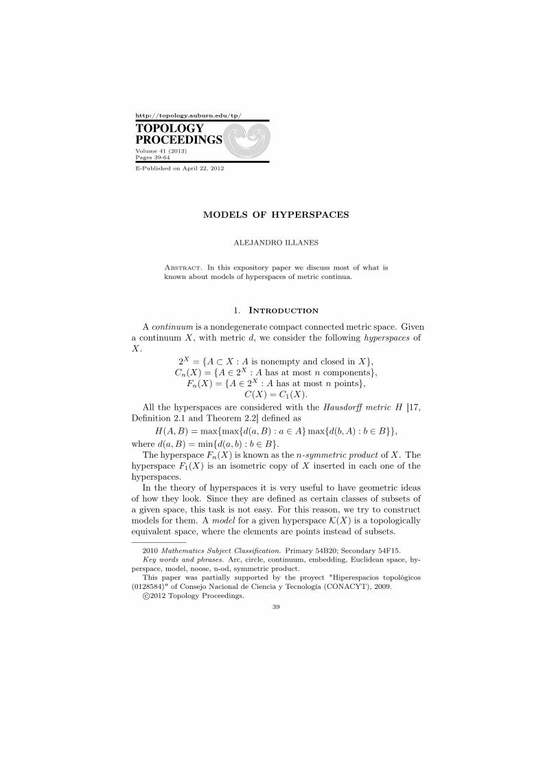
C([0, 1]) = {[a, b] : 0 ≤ a ≤ b ≤ 1}.

It is easy to check that the function ϕ : C([0, 1]) → R2 (R2 is theEuclidean plane) given by ϕ([a, b]) = (a, b) is a homeomorphism betweenC([0, 1]) and the triangle T = {(a, b) ∈ R2 : 0 ≤ a ≤ b ≤ 1}, representedin Figure 1.

Figure 1

Thus, we can say that this triangle is a model for C([0, 1]). Observethat the set of elements in C([0, 1]) that contain 0 (intervals of the form[0, b]) is represented by an edge of T . Similarly, the set of elements ofC([0, 1]) containing 1 is represented by another edge of T . The set ofsingletons F1([0, 1]) is represented on the third edge of T (the diagonal).

MODELS OF HYPERSPACES 41

Sometimes it is more useful to represent C([0, 1]) by using the mapψ : C([0, 1])→ R2 given by ψ([a, b]) = (a+b2 , b−a). Notice that the imageof ψ is the triangle illustrated in Figure 2.

Figure 2

3. The circle, C(X)

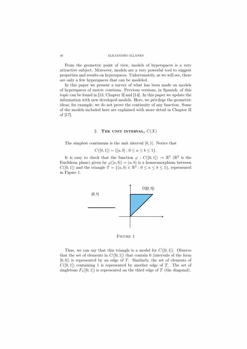
Let S1 be the unit circle in R2, centered at the origin. For each subarcA of S1 let m(A) be the middle point of A in S1 and let L(A) be thelength of A. Then define ϕ : C(S1)→ R2 by

ϕ(A) =

{[1− (L(A)/2π)]m(A), if A 6= S1,(0, 0), if A = S1.

It is easy to check that ϕ is a homeomorphism between C(S1) and theunit disc. Thus, a model for C(S1) is this disc.

Figure 3

Take a point p ∈ S1. For later use, we need to identify the image underϕ of the set C = {A ∈ C(S1) : p ∈ A}. By the homogeneity of S1 wesuppose that p = (0, 1). The best way to visualize C is recognizing itsboundary, which is given by the set {A ∈ C(S1) : A is a subarc of S1


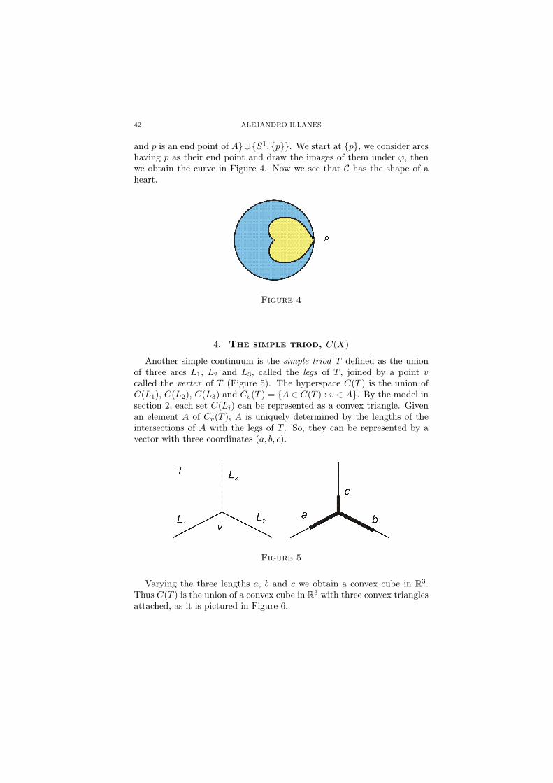
and p is an end point of A}∪{S1, {p}}. We start at {p}, we consider arcshaving p as their end point and draw the images of them under ϕ, thenwe obtain the curve in Figure 4. Now we see that C has the shape of aheart.

Figure 4

4. The simple triod, C(X)

Another simple continuum is the simple triod T defined as the unionof three arcs L1, L2 and L3, called the legs of T , joined by a point vcalled the vertex of T (Figure 5). The hyperspace C(T ) is the union ofC(L1), C(L2), C(L3) and Cv(T ) = {A ∈ C(T ) : v ∈ A}. By the model insection 2, each set C(Li) can be represented as a convex triangle. Givenan element A of Cv(T ), A is uniquely determined by the lengths of theintersections of A with the legs of T . So, they can be represented by avector with three coordinates (a, b, c).

Figure 5

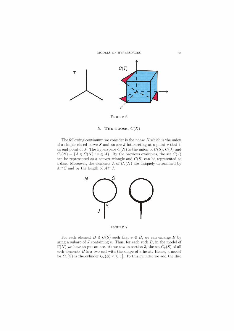
Varying the three lengths a, b and c we obtain a convex cube in R3.Thus C(T ) is the union of a convex cube in R3 with three convex trianglesattached, as it is pictured in Figure 6.


Figure 6

5. The noose, C(X)

The following continuum we consider is the noose N which is the unionof a simple closed curve S and an arc J intersecting at a point v that isan end point of J . The hyperspace C(N) is the union of C(S), C(J) andCv(N) = {A ∈ C(N) : v ∈ A}. By the previous examples, the set C(J)can be represented as a convex triangle and C(S) can be represented asa disc. Moreover, the elements A of Cv(N) are uniquely determined byA ∩ S and by the length of A ∩ J .

Figure 7

For each element B ∈ C(S) such that v ∈ B, we can enlarge B byusing a subarc of J containing v. Thus, for each such B, in the model ofC(N) we have to put an arc. As we saw in section 3, the set Cv(S) of allsuch elements B is a two cell with the shape of a heart. Hence, a modelfor Cv(S) is the cylinder Cv(S)× [0, 1]. To this cylinder we add the disc


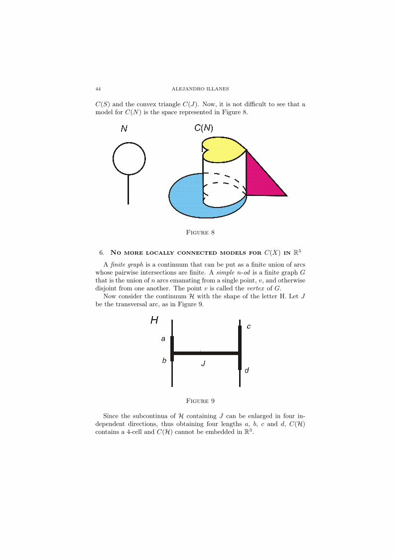
C(S) and the convex triangle C(J). Now, it is not difficult to see that amodel for C(N) is the space represented in Figure 8.

Figure 8

6. No more locally connected models for C(X) in R3

A finite graph is a continuum that can be put as a finite union of arcswhose pairwise intersections are finite. A simple n-od is a finite graph Gthat is the union of n arcs emanating from a single point, v, and otherwisedisjoint from one another. The point v is called the vertex of G.

Now consider the continuum H with the shape of the letter H. Let Jbe the transversal arc, as in Figure 9.

Figure 9

Since the subcontinua of H containing J can be enlarged in four in-dependent directions, thus obtaining four lengths a, b, c and d, C(H)contains a 4-cell and C(H) cannot be embedded in R3.


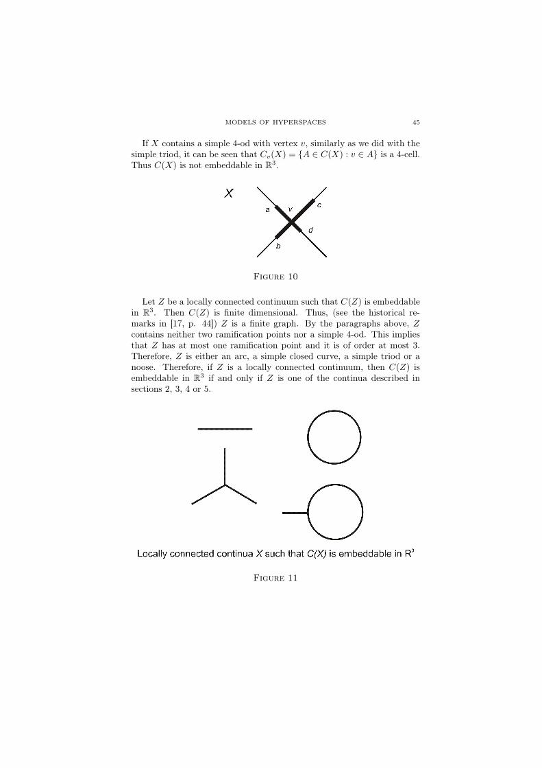
If X contains a simple 4-od with vertex v, similarly as we did with thesimple triod, it can be seen that Cv(X) = {A ∈ C(X) : v ∈ A} is a 4-cell.Thus C(X) is not embeddable in R3.

Figure 10

Let Z be a locally connected continuum such that C(Z) is embeddablein R3. Then C(Z) is finite dimensional. Thus, (see the historical re-marks in [17, p. 44]) Z is a finite graph. By the paragraphs above, Zcontains neither two ramification points nor a simple 4-od. This impliesthat Z has at most one ramification point and it is of order at most 3.Therefore, Z is either an arc, a simple closed curve, a simple triod or anoose. Therefore, if Z is a locally connected continuum, then C(Z) isembeddable in R3 if and only if Z is one of the continua described insections 2, 3, 4 or 5.

Figure 11


7. More continua X for which C(X) is embeddable in R3

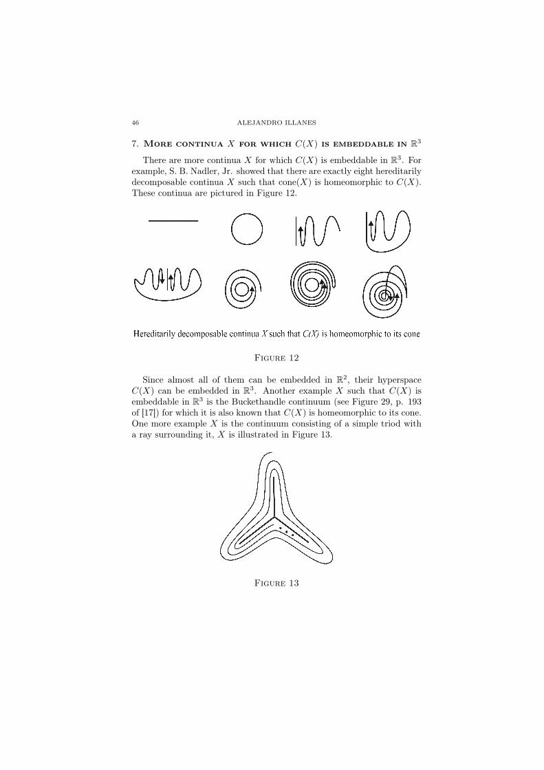
There are more continua X for which C(X) is embeddable in R3. Forexample, S. B. Nadler, Jr. showed that there are exactly eight hereditarilydecomposable continua X such that cone(X) is homeomorphic to C(X).These continua are pictured in Figure 12.

Figure 12

Since almost all of them can be embedded in R2, their hyperspaceC(X) can be embedded in R3. Another example X such that C(X) isembeddable in R3 is the Buckethandle continuum (see Figure 29, p. 193of [17]) for which it is also known that C(X) is homeomorphic to its cone.One more example X is the continuum consisting of a simple triod witha ray surrounding it, X is illustrated in Figure 13.

Figure 13


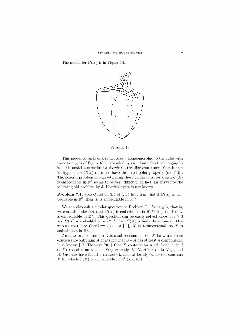
The model for C(X) is in Figure 14.

Figure 14

This model consists of a solid rocket (homeomorphic to the cube withthree triangles of Figure 6) surrounded by an infinite sheet converging toit. This model was useful for showing a tree-like continuum X such thatits hyperspace C(X) does not have the fixed point property (see [15]).The general problem of characterizing those continua X for which C(X)is embeddable in R3 seems to be very difficult. In fact, an answer to thefollowing old problem by J. Krazinkiewicz is not known.

Problem 7.1. (see Question 3.5 of [24]) Is it true that if C(X) is em-beddable in R3, then X is embeddable in R2?

We can also ask a similar question as Problem 7.1 for n ≥ 3, that is,we can ask if the fact that C(X) is embeddable in Rn+1 implies that Xis embeddable in Rn. This question can be easily solved since if n ≥ 3and C(X) is embeddable in Rn+1, then C(X) is finite dimensional. Thisimplies that (see Corollary 73.11 of [17]) X is 1-dimensional, so X isembeddable in R3.

An n-od in a continuum X is a subcontinuum B of X for which thereexists a subcontinuum A of B such that B−A has at least n components.It is known [17, Theorem 70.1] that X contains an n-od if and only ifC(X) contains an n-cell. Very recently, V. Martínez de la Vega andN. Ordoñez have found a characterization of locally connected continuaX for which C(X) is embeddable in R4 (and R5).


8. Locally connected continua X for which C(X) isembeddable in R4 and R5

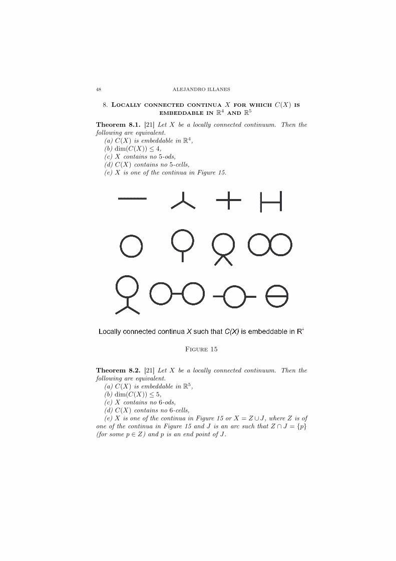
Theorem 8.1. [21] Let X be a locally connected continuum. Then thefollowing are equivalent.

(a) C(X) is embeddable in R4,(b) dim(C(X)) ≤ 4,(c) X contains no 5-ods,(d) C(X) contains no 5-cells,(e) X is one of the continua in Figure 15.

Figure 15

Theorem 8.2. [21] Let X be a locally connected continuum. Then thefollowing are equivalent.

(a) C(X) is embeddable in R5,(b) dim(C(X)) ≤ 5,(c) X contains no 6-ods,(d) C(X) contains no 6-cells,(e) X is one of the continua in Figure 15 or X = Z ∪ J , where Z is of

one of the continua in Figure 15 and J is an arc such that Z ∩ J = {p}(for some p ∈ Z) and p is an end point of J .


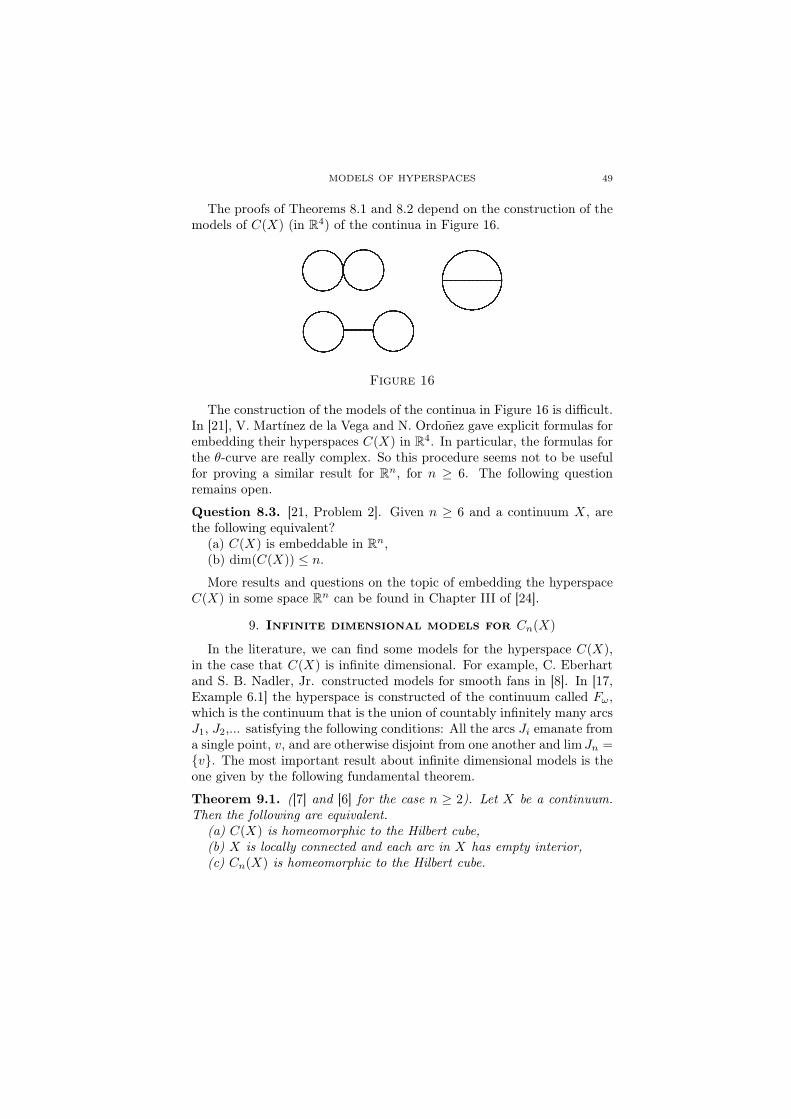
The proofs of Theorems 8.1 and 8.2 depend on the construction of themodels of C(X) (in R4) of the continua in Figure 16.

Figure 16

The construction of the models of the continua in Figure 16 is difficult.In [21], V. Martínez de la Vega and N. Ordoñez gave explicit formulas forembedding their hyperspaces C(X) in R4. In particular, the formulas forthe θ-curve are really complex. So this procedure seems not to be usefulfor proving a similar result for Rn, for n ≥ 6. The following questionremains open.

Question 8.3. [21, Problem 2]. Given n ≥ 6 and a continuum X, arethe following equivalent?

(a) C(X) is embeddable in Rn,(b) dim(C(X)) ≤ n.

More results and questions on the topic of embedding the hyperspaceC(X) in some space Rn can be found in Chapter III of [24].

9. Infinite dimensional models for Cn(X)

In the literature, we can find some models for the hyperspace C(X),in the case that C(X) is infinite dimensional. For example, C. Eberhartand S. B. Nadler, Jr. constructed models for smooth fans in [8]. In [17,Example 6.1] the hyperspace is constructed of the continuum called Fω,which is the continuum that is the union of countably infinitely many arcsJ1, J2,... satisfying the following conditions: All the arcs Ji emanate froma single point, v, and are otherwise disjoint from one another and lim Jn ={v}. The most important result about infinite dimensional models is theone given by the following fundamental theorem.

Theorem 9.1. ([7] and [6] for the case n ≥ 2). Let X be a continuum.Then the following are equivalent.

(a) C(X) is homeomorphic to the Hilbert cube,(b) X is locally connected and each arc in X has empty interior,(c) Cn(X) is homeomorphic to the Hilbert cube.


10. Cn([0, 1]) for n ≥ 2

R. M. Schori has shown that C2([0, 1]) is a 4-cell by using the followingargument [10, Lemma 2.2]. Let C1

0 = {A ∈ C2([0, 1]) : 0, 1 ∈ A} andC1 = {A ∈ C2([0, 1]) : 1 ∈ A}. The typical elements of C1

0 are of the formA = [0, a] ∪ [b, 1], where 0 ≤ a ≤ b ≤ 1. We can define ϕ(A) = (a, b).Then ϕ is not a function since ϕ([0, 1]) = ϕ([0, a]∪ [a, 1]) = (a, a) for eacha ∈ [0, 1]. The image of ϕ is the triangle T in Figure 1. If we identify thediagonal ∆ of T to a point we obtain the space T/∆ and now ϕ is a welldefined homeomorphism between C1

0 and T/∆. This proves that C10 is a

2-cell. It is easy to show that the function ψ : C10 × [0, 1] → C1 given by

ψ(A, t) = t+(1− t)A is continuous, surjective and its only nondegeneratefiber is the set C1

0 × {1}. Thus, C1 is homeomorphic to the cone ofC1

0 . Hence, C1 is a 3-cell. Finally, the function σ : C1× [0, 1]→ C2([0, 1])given by σ(A, t) = tA is continuous, surjective and its only nondegeneratefiber is C1 × {0}. Hence, C2([0, 1]) is homeomorphic to the cone over C1.Therefore, C2([0, 1]) is a 4-cell.

In [11], it has been shown that, if n ≥ 3, then {A ∈ Cn([0, 1]) : A hasa neighborhood in Cn(X) that is a 2n-cell} = Cn([0, 1]) − Cn−1([0, 1]).In particular, this implies that Cn([0, 1]) is not a 2n-cell. The author hasconstructed a model for C3([0, 1]) and he is able to show that C3([0, 1])can be embedded in R6. The following problem remains unsolved.

Problem 10.1. Is Cn([0, 1]) embeddable in R2n for each (for some) n ≥4?

11. Cn(S1) for n ≥ 2

In [12] it is shown that C2(S1) is the cone over a solid torus. The proofis difficult and it seems that it cannot be generalized for n ≥ 3. Nothingelse is known for Cn(S1) (n ≥ 3). The following questions are interesting.

Problem 11.1. (a) Find a model for C3(S1); (b) Is Cn(S1) the cone overa continuum for some (for all) n ≥ 3?; (c) Is Cn(S1) embeddable in R2n

for each (for some) n ≥ 3?

In [19, Theorem 3.1] it was shown that if X is a simple m-od, thenC(X) is the cone over the set {A ∈ Cn(X) : A contains an end pointof X}. In [20] V. Martínez de la Vega proved that if G is a finite graphsuch that Cn(G) is a cone for some n ≥ 2, then G is either an m-odor a simple closed curve. So, the answer to Problem2.8 (b) could give acharacterization of those finite graphs G for which Cn(G) is a cone.


12. Models for 2X

In the early 1920’s, in Poland it was conjectured that 2[0,1] is a Hilbertcube. It was not until the 1970’s when this problem was solved by D. W.Curtis and R. M. Schori who proved the following fundamental theorem.

Theorem 12.1. [7]. Let X be a continuum. Then the following areequivalent.

(a) X is locally connected,(b) 2X is homeomorphic to the Hilbert cube.

Although models of some very specific examples have been constructedfor 2X , the only significant result about models for 2X is Theorem 12.1.

13. The unit interval, Fn(X)

As before, in the topic of models, the simplest continuum is the unitinterval [0, 1].

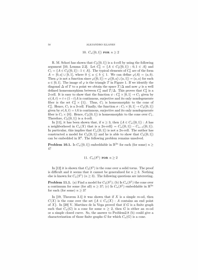
Let ϕ : F2([0, 1])→ R2 be given by ϕ({a, b}) = (min{a, b},max{a, b}).Clearly, ϕ is an embedding whose image is the convex triangle {(a, b) ∈R2 : 0 ≤ a ≤ b ≤ 1}. Thus, F2([0, 1]) is a 2-cell.

Figure 17

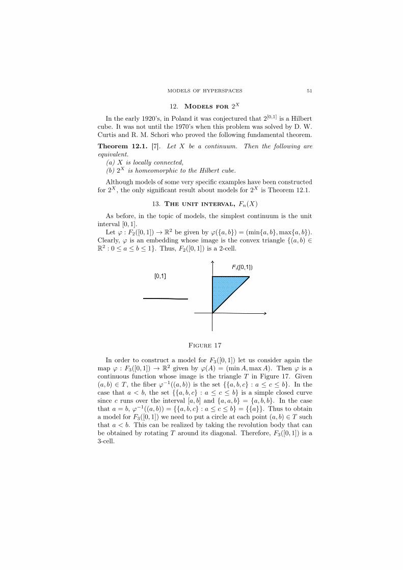
In order to construct a model for F3([0, 1]) let us consider again themap ϕ : F3([0, 1]) → R2 given by ϕ(A) = (minA,maxA). Then ϕ is acontinuous function whose image is the triangle T in Figure 17. Given(a, b) ∈ T , the fiber ϕ−1((a, b)) is the set {{a, b, c} : a ≤ c ≤ b}. In thecase that a < b, the set {{a, b, c} : a ≤ c ≤ b} is a simple closed curvesince c runs over the interval [a, b] and {a, a, b} = {a, b, b}. In the casethat a = b, ϕ−1((a, b)) = {{a, b, c} : a ≤ c ≤ b} = {{a}}. Thus to obtaina model for F3([0, 1]) we need to put a circle at each point (a, b) ∈ T suchthat a < b. This can be realized by taking the revolution body that canbe obtained by rotating T around its diagonal. Therefore, F3([0, 1]) is a3-cell.


Figure 18

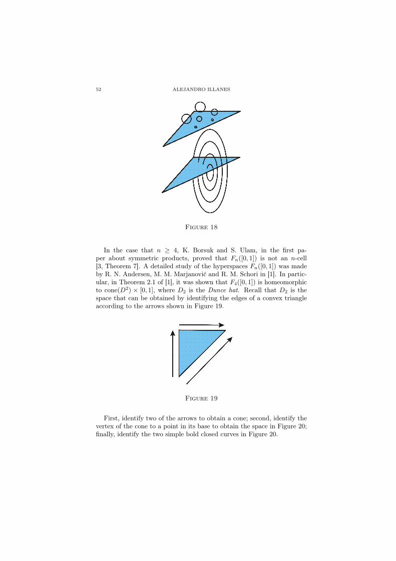
In the case that n ≥ 4, K. Borsuk and S. Ulam, in the first pa-per about symmetric products, proved that Fn([0, 1]) is not an n-cell[3, Theorem 7]. A detailed study of the hyperspaces Fn([0, 1]) was madeby R. N. Andersen, M. M. Marjanović and R. M. Schori in [1]. In partic-ular, in Theorem 2.1 of [1], it was shown that F4([0, 1]) is homeomorphicto cone(D2) × [0, 1], where D2 is the Dunce hat. Recall that D2 is thespace that can be obtained by identifying the edges of a convex triangleaccording to the arrows shown in Figure 19.

Figure 19

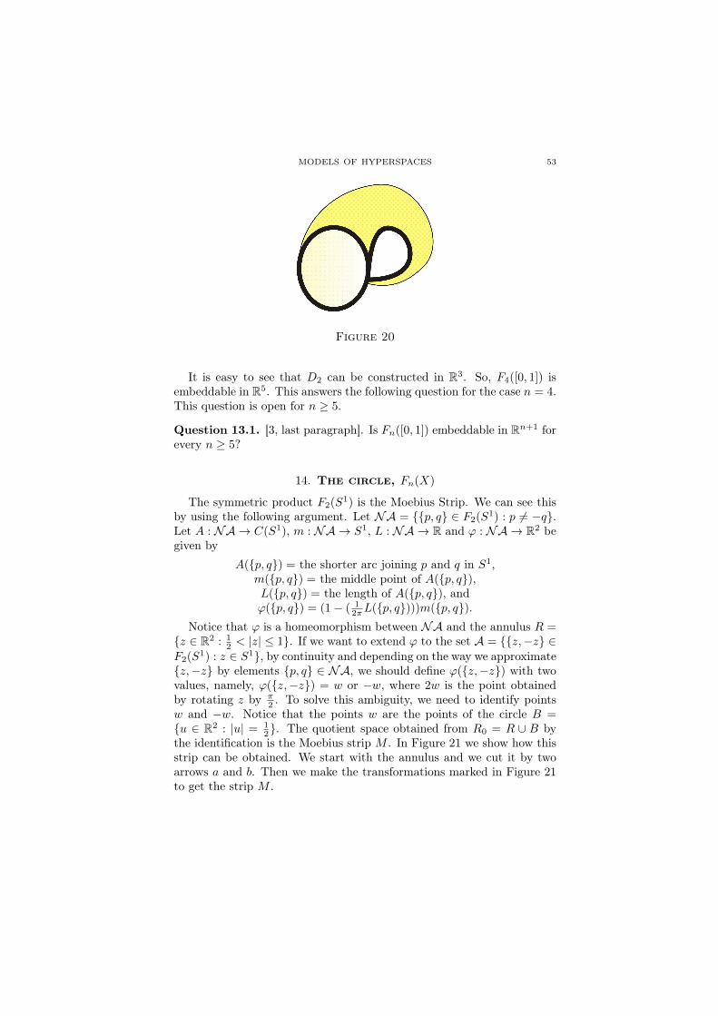
First, identify two of the arrows to obtain a cone; second, identify thevertex of the cone to a point in its base to obtain the space in Figure 20;finally, identify the two simple bold closed curves in Figure 20.


Figure 20

It is easy to see that D2 can be constructed in R3. So, F4([0, 1]) isembeddable in R5. This answers the following question for the case n = 4.This question is open for n ≥ 5.

Question 13.1. [3, last paragraph]. Is Fn([0, 1]) embeddable in Rn+1 forevery n ≥ 5?

14. The circle, Fn(X)

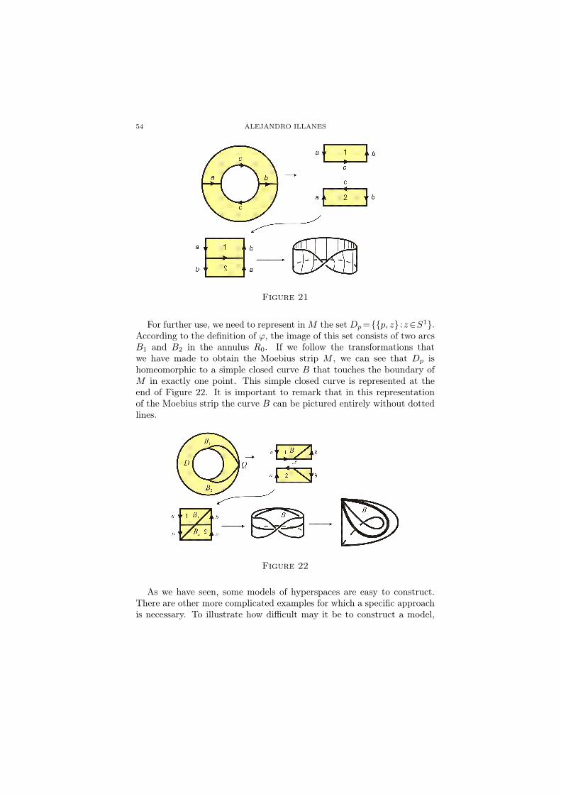
The symmetric product F2(S1) is the Moebius Strip. We can see thisby using the following argument. Let NA = {{p, q} ∈ F2(S1) : p 6= −q}.Let A : NA → C(S1), m : NA → S1, L : NA → R and ϕ : NA → R2 begiven by

A({p, q}) = the shorter arc joining p and q in S1,m({p, q}) = the middle point of A({p, q}),L({p, q}) = the length of A({p, q}), andϕ({p, q}) = (1− ( 1

2πL({p, q})))m({p, q}).Notice that ϕ is a homeomorphism between NA and the annulus R =

{z ∈ R2 : 12 < |z| ≤ 1}. If we want to extend ϕ to the set A = {{z,−z} ∈

F2(S1) : z ∈ S1}, by continuity and depending on the way we approximate{z,−z} by elements {p, q} ∈ NA, we should define ϕ({z,−z}) with twovalues, namely, ϕ({z,−z}) = w or −w, where 2w is the point obtainedby rotating z by π

2 . To solve this ambiguity, we need to identify pointsw and −w. Notice that the points w are the points of the circle B ={u ∈ R2 : |u| = 1

2}. The quotient space obtained from R0 = R ∪ B bythe identification is the Moebius strip M . In Figure 21 we show how thisstrip can be obtained. We start with the annulus and we cut it by twoarrows a and b. Then we make the transformations marked in Figure 21to get the strip M .


Figure 21

For further use, we need to represent inM the set Dp={{p, z} :z∈S1}.According to the definition of ϕ, the image of this set consists of two arcsB1 and B2 in the annulus R0. If we follow the transformations thatwe have made to obtain the Moebius strip M , we can see that Dp ishomeomorphic to a simple closed curve B that touches the boundary ofM in exactly one point. This simple closed curve is represented at theend of Figure 22. It is important to remark that in this representationof the Moebius strip the curve B can be pictured entirely without dottedlines.

Figure 22

As we have seen, some models of hyperspaces are easy to construct.There are other more complicated examples for which a specific approachis necessary. To illustrate how difficult may it be to construct a model,


let us mention that K. Borsuk made a mistake. He published a paper[2] claiming that F3(S1) is homeomorphic to S1 × S2, where Sn is theunit sphere in Rn+1. Three years later, R. Bott [4] corrected this factby proving that F3(S1) is homeomorphic to S3. J. Mostovoy pointed outthat an interesting illustration of the non-triviality of Bott’s theorem isthe result attributed to E. Schepin which says that the embedding knot(F1(S1)) is a trefoil knot (see Theorem 2 of [23]).

Even when no models for Fn(S1) (n ≥ 4) have been constructed, in [25]and [27] some topological properties of these spaces have been studied.

15. The simple triod, F2(X)

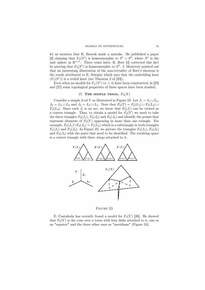
Consider a simple 3-od Y as illustrated in Figure 23. Let J1 = L1∪L2,J2 = L2 ∪ L3 and J3 = L3 ∪ L1. Note that F2(T ) = F2(L1) ∪ F2(L2) ∪F2(L3). Since each Ji is an arc, we know that F2(Ji) can be viewed asa convex triangle. Thus, to obtain a model for F2(Y ) we need to takethe three triangles F2(J1), F2(J2) and F2(J3) and identify the points thatrepresent elements of F2(Y ) appearing in more than one triangle. Forexample, F2(J1)∩F2(J2) = F2(L2) which is a subtriangle in both trianglesF2(J1) and F2(J2). In Figure 23, we picture the triangles F2(J1), F2(J2)and F2(J3) with the parts that need to be identified. The resulting spaceis a convex triangle with three wings attached to it.

Figure 23

E. Castañeda has recently found a model for F3(Y ) [26]. He showedthat F3(Y ) is the cone over a torus with four disks attached to it, one asan "equator" and the three other ones as "meridians" (Figure 24).


Figure 24

16. The simple 4-od, F2(X)

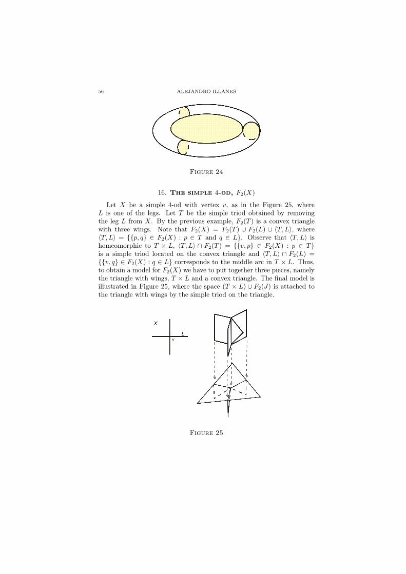
Let X be a simple 4-od with vertex v, as in the Figure 25, whereL is one of the legs. Let T be the simple triod obtained by removingthe leg L from X. By the previous example, F2(T ) is a convex trianglewith three wings. Note that F2(X) = F2(T ) ∪ F2(L) ∪ 〈T, L〉, where〈T, L〉 = {{p, q} ∈ F2(X) : p ∈ T and q ∈ L}. Observe that 〈T, L〉 ishomeomorphic to T × L, 〈T, L〉 ∩ F2(T ) = {{v, p} ∈ F2(X) : p ∈ T}is a simple triod located on the convex triangle and 〈T, L〉 ∩ F2(L) ={{v, q} ∈ F2(X) : q ∈ L} corresponds to the middle arc in T × L. Thus,to obtain a model for F2(X) we have to put together three pieces, namelythe triangle with wings, T × L and a convex triangle. The final model isillustrated in Figure 25, where the space (T × L) ∪ F2(J) is attached tothe triangle with wings by the simple triod on the triangle.

Figure 25


17. The noose, F2(X)

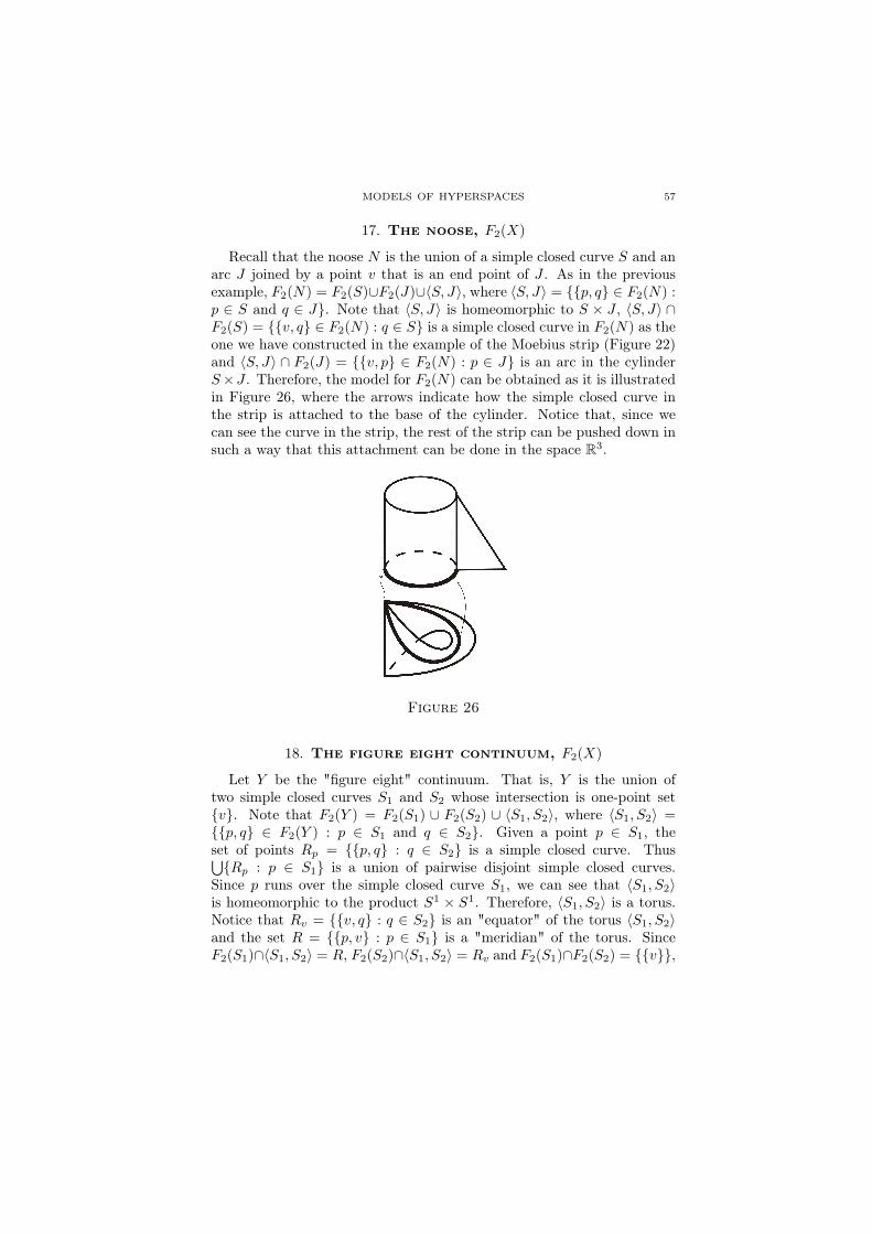
Recall that the noose N is the union of a simple closed curve S and anarc J joined by a point v that is an end point of J . As in the previousexample, F2(N) = F2(S)∪F2(J)∪〈S, J〉, where 〈S, J〉 = {{p, q} ∈ F2(N) :p ∈ S and q ∈ J}. Note that 〈S, J〉 is homeomorphic to S × J , 〈S, J〉 ∩F2(S) = {{v, q} ∈ F2(N) : q ∈ S} is a simple closed curve in F2(N) as theone we have constructed in the example of the Moebius strip (Figure 22)and 〈S, J〉 ∩ F2(J) = {{v, p} ∈ F2(N) : p ∈ J} is an arc in the cylinderS×J . Therefore, the model for F2(N) can be obtained as it is illustratedin Figure 26, where the arrows indicate how the simple closed curve inthe strip is attached to the base of the cylinder. Notice that, since wecan see the curve in the strip, the rest of the strip can be pushed down insuch a way that this attachment can be done in the space R3.

Figure 26

18. The figure eight continuum, F2(X)

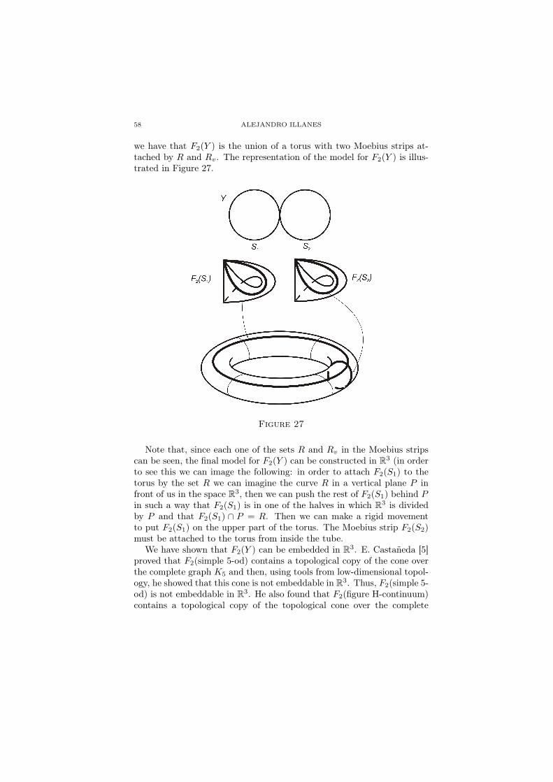
Let Y be the "figure eight" continuum. That is, Y is the union oftwo simple closed curves S1 and S2 whose intersection is one-point set{v}. Note that F2(Y ) = F2(S1) ∪ F2(S2) ∪ 〈S1, S2〉, where 〈S1, S2〉 ={{p, q} ∈ F2(Y ) : p ∈ S1 and q ∈ S2}. Given a point p ∈ S1, theset of points Rp = {{p, q} : q ∈ S2} is a simple closed curve. Thus⋃{Rp : p ∈ S1} is a union of pairwise disjoint simple closed curves.

Since p runs over the simple closed curve S1, we can see that 〈S1, S2〉is homeomorphic to the product S1 × S1. Therefore, 〈S1, S2〉 is a torus.Notice that Rv = {{v, q} : q ∈ S2} is an "equator" of the torus 〈S1, S2〉and the set R = {{p, v} : p ∈ S1} is a "meridian" of the torus. SinceF2(S1)∩〈S1, S2〉 = R, F2(S2)∩〈S1, S2〉 = Rv and F2(S1)∩F2(S2) = {{v}},


we have that F2(Y ) is the union of a torus with two Moebius strips at-tached by R and Rv. The representation of the model for F2(Y ) is illus-trated in Figure 27.

Figure 27

Note that, since each one of the sets R and Rv in the Moebius stripscan be seen, the final model for F2(Y ) can be constructed in R3 (in orderto see this we can image the following: in order to attach F2(S1) to thetorus by the set R we can imagine the curve R in a vertical plane P infront of us in the space R3, then we can push the rest of F2(S1) behind Pin such a way that F2(S1) is in one of the halves in which R3 is dividedby P and that F2(S1) ∩ P = R. Then we can make a rigid movementto put F2(S1) on the upper part of the torus. The Moebius strip F2(S2)must be attached to the torus from inside the tube.

We have shown that F2(Y ) can be embedded in R3. E. Castañeda [5]proved that F2(simple 5-od) contains a topological copy of the cone overthe complete graph K5 and then, using tools from low-dimensional topol-ogy, he showed that this cone is not embeddable in R3. Thus, F2(simple 5-od) is not embeddable in R3. He also found that F2(figure H-continuum)contains a topological copy of the topological cone over the complete


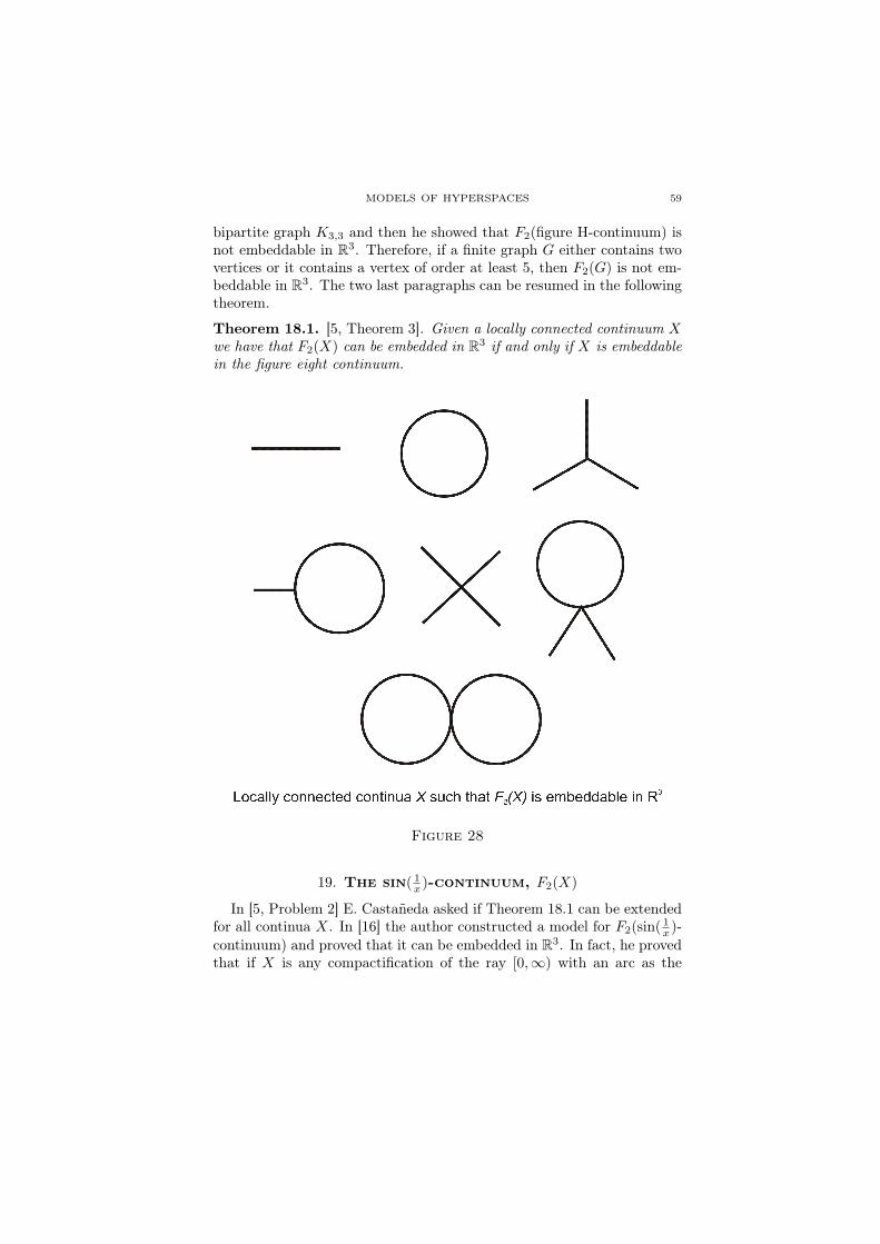
bipartite graph K3,3 and then he showed that F2(figure H-continuum) isnot embeddable in R3. Therefore, if a finite graph G either contains twovertices or it contains a vertex of order at least 5, then F2(G) is not em-beddable in R3. The two last paragraphs can be resumed in the followingtheorem.

Theorem 18.1. [5, Theorem 3]. Given a locally connected continuum Xwe have that F2(X) can be embedded in R3 if and only if X is embeddablein the figure eight continuum.

Figure 28

19. The sin( 1x )-continuum, F2(X)

In [5, Problem 2] E. Castañeda asked if Theorem 18.1 can be extendedfor all continua X. In [16] the author constructed a model for F2(sin( 1

x )-continuum) and proved that it can be embedded in R3. In fact, he provedthat if X is any compactification of the ray [0,∞) with an arc as the


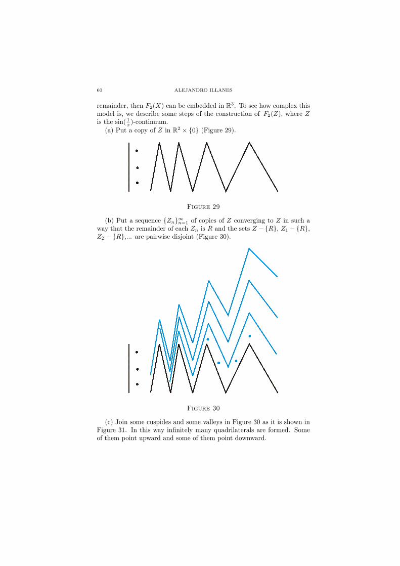
remainder, then F2(X) can be embedded in R3. To see how complex thismodel is, we describe some steps of the construction of F2(Z), where Zis the sin( 1

x )-continuum.(a) Put a copy of Z in R2 × {0} (Figure 29).

Figure 29

(b) Put a sequence {Zn}∞n=1 of copies of Z converging to Z in such away that the remainder of each Zn is R and the sets Z − {R}, Z1 − {R},Z2 − {R},... are pairwise disjoint (Figure 30).

Figure 30

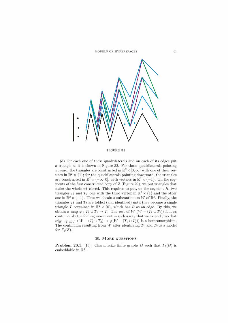
(c) Join some cuspides and some valleys in Figure 30 as it is shown inFigure 31. In this way infinitely many quadrilaterals are formed. Someof them point upward and some of them point downward.


Figure 31

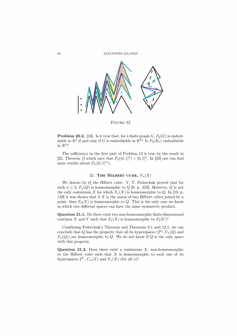
(d) For each one of these quadrilaterals and on each of its edges puta triangle as it is shown in Figure 32. For those quadrilaterals pointingupward, the triangles are constructed in R2× [0,∞) with one of their ver-tices in R2 × {1}; for the quadrilaterals pointing downward, the trianglesare constructed in R2× (−∞, 0], with vertices in R2×{−1}. On the seg-ments of the first constructed copy of Z (Figure 29), we put triangles thatmake the whole set closed. This requires to put, on the segment R, twotriangles T1 and T2, one with the third vertex in R2 × {1} and the otherone in R2×{−1}. Thus we obtain a subcontinuum W of R3. Finally, thetriangles T1 and T2 are folded (and identified) until they become a singletriangle T contained in R2 × {0}, which has R as an edge. By this, weobtain a map ϕ : T1 ∪ T2 → T . The rest of W (W − (T1 ∪ T2)) followscontinuously the folding movement in such a way that we extend ϕ so thatϕ|W−(T1∪T2) : W − (T1 ∪ T2) → ϕ(W − (T1 ∪ T2)) is a homeomorphism.The continuum resulting from W after identifying T1 and T2 is a modelfor F2(Z).

20. More questions

Problem 20.1. [16]. Characterize finite graphs G such that F2(G) isembeddable in R4.


Figure 32

Problem 20.2. [16]. Is it true that, for a finite graph G, F2(G) is embed-dable in R4 if and only if G is embeddable in R2? Is F2(K5) embeddablein R4?

The sufficiency in the first part of Problem 12 is true by the result in[22, Theorem 1] which says that F2([0, 1]2) = [0, 1]4. In [22] one can findmore results about F2([0, 1]m).

21. The Hilbert cube, Fn(X)

We denote by Q the Hilbert cube. V. V. Fedorchuk proved that foreach n ≥ 2, Fn(Q) is homeomorphic to Q [9, p. 223]. However, Q is notthe only continuum X for which Fn(X) is homeomorphic to Q. In [18, p.139] it was shown that if X is the union of two Hilbert cubes joined by apoint, then F2(X) is homeomorphic to Q. This is the only case we knowin which two different spaces can have the same symmetric product.

Question 21.1. Do there exist two non-homeomorphic finite-dimensionalcontinua X and Y such that F2(X) is homeomorphic to F2(Y )?

Combining Fedorchuk’s Theorem and Theorems 9.1 and 12.1, we canconclude that Q has the property that all its hyperspaces (2Q, Cn(Q) andFn(Q)) are homeomorphic to Q. We do not know if Q is the only spacewith this property.

Question 21.2. Does there exist a continuum X, non-homeomorphicto the Hilbert cube such that X is homeomorphic to each one of itshyperspaces 2X , Cn(X) and Fn(X) (for all n)?


References

[1] R. N. Andersen, M. M. Marjanović and R. M. Schori, Symmetric products andhigher dimensional products, Topology Proc. 18 (1993), 7–17.

[2] K. Borsuk, On the third symmetric potency of the circumference, Fund. Math. 36(1949), 235–244.

[3] K. Borsuk and S. Ulam, On symmetric products of topological spaces, Bull. Amer.Math. Soc. 37 (1931), 875–882.

[4] R. Bott, On the third symmetric potency of S1, Fund. Math. 39 (1952), 364–368.[5] E. Castañeda, Embedding symmetric products in Euclidean spaces, Continuum

Theory (Denton, TX, 1999), 67–79, Lectures Notes in Pure and Appl. Math.,230, Dekker, New York, 2002.

[6] D. Curtis, Growth hyperspaces of Peano continua, Trans. Amer. Math. Soc. 238(1978), 271–283.

[7] D. Curtis and R. M. Schori, Hyperspaces of Peano continua are Hilbert cubes,Fund. Math. 101 (1978), 19–38.

[8] C. Eberhart and S. B. Nadler, Jr., Hyperspaces of cones and fans, Proc. Amer.Math. Soc. 77 (1979), 279–288.

[9] V. V. Fedorchuk, Covariant functors in the category of compacta, absolute re-tracts, and Q–manifolds, Russian Math. Surveys 36:3 (1981), 211–233.

[10] A. Illanes, The hyperspace C2(X) for a finite graph X is unique, Glas. Mat. Ser.III 37(57) (2002), 347–363.

[11] A. Illanes, Finite graphs X have unique hyperspaces Cn(X), Topology Proc. 27(2003), 179–188.

[12] A. Illanes, A model for the hyperspace C2(S1), Questions Answers Gen. Topology22 (2004), 117–130.

[13] A. Illanes, Hyperspaces of continua (Hiperespacios de continuos) (Span-ish), Aportaciones Matemáticas, Textos 28 (Nivel Medio). Mexico: SociedadMatemática Mexicana. (2004).

[14] A. Illanes, Modelos de hiperespacios (Spanish), Aportaciones Matemáticas, Textos31 (Nivel Medio). México: Sociedad Matemática Mexicana (2006).

[15] A. Illanes, A tree-like continuum whose hyperspace of subcontinua admits a fixed-point-free map, Topology Proc. 32 (2008), 55–74.

[16] A Illanes, A nonlocally connected continuum whose second symmetric product canbe embedded in R3, Questions Answers Gen. Topology 26 (2008), 115–119.

[17] A. Illanes and S. B. Nadler, Jr., Hyperspaces: Fundamentals and Recent Advances,Monographs and Textbooks in Pure and Applied Mathematics, Vol. 216, MarcelDekker, Inc., New York and Basel, 1999.

[18] A. Illanes, S. Macías and S. B. Nadler, Jr., Symmetric Products and Q-manifolds,Geometry and Topology in Dynamics, Contemporary Math. Series of Amer. Math.Soc., Vol. 246, 1999, Providence, RI, 137–141.

[19] S. Macías, Fans whose hyperspaces are cones, Topology Proc. 27 (2003), 217–222.[20] V. Martínez-de-la-Vega, Dimension of n-fold hyperspaces of graphs, Houston J.

Math. 32 (2006), 783–799.[21] V. Martínez-de-la-Vega and N. Ordoñez, Embedding hyperspaces, Topology Appl.

159 (2012), 2021–2232.[22] R. Molski, On symmetric products, Fund. Math. 44 (1957), 165–170.[23] J. Mostovoy, Latices in C and finite subsets of a circle, Amer. Math. Montly 111

(2004), 357–360.


[24] S. B. Nadler, Jr., Hyperspaces of sets: A text with research questions, Monographsand Textbooks in Pure and Applied Mathematics, Vol. 49, Marcel Dekker, Inc.,New York and Basel, 1978.

[25] C. Tuffley, Finite subset spaces of S1, Algebr. Geom. Topol. 2 (2002), 1119–1145.[26] P. I. Vidal Escobar, Los hiperespacios de continuos desde el punto de vista de sus

modelos geométricos, Bachelor Thesis, Director: Enrique Castañeda, UniversidadAutónoma del Estado de México, August, 2009.

[27] W. Wu, Note sur les produits essentiels symétriques des espaces topologique, I,(French) Comptes Rendus des Séances de l’Académie des Sciences 16 (1947),1139–1141.

Instituto de Matemáticas, Universidad Nacional Autónoma de México,Circuito Exterior, Cd. Universitaria, México, 04510, D.F.

E-mail address: [email protected]

Date post:	20-Nov-2021
Category:	Documents
Upload:	others
View:	2 times
Download:	0 times

Volume 41, 2013 Pages 39{64

Documents