Taku Komura Volume Rendering & Classification 1 Visualisation : Lecture 10 Visualisation – Lecture 10 Taku Komura Institute for Perception, Action & Behaviour School of Informatics Volume Rendering & Classification
Transcript
Taku Komura Volume Rendering & Classification 1
Visualisation : Lecture 10
Visualisation – Lecture 10
Taku Komura
Institute for Perception, Action & BehaviourSchool of Informatics
Volume Rendering & Classification
Taku Komura Volume Rendering & Classification 2
Visualisation : Lecture 10
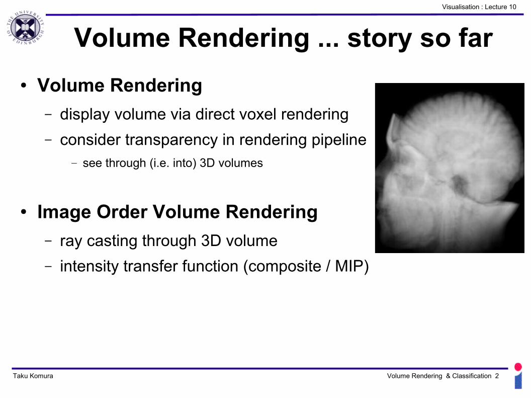
Volume Rendering ... story so far● Volume Rendering
– display volume via direct voxel rendering– consider transparency in rendering pipeline
— see through (i.e. into) 3D volumes
● Image Order Volume Rendering– ray casting through 3D volume– intensity transfer function (composite / MIP)
Taku Komura Volume Rendering & Classification 3
Visualisation : Lecture 10
Volume Classification● Requirement : map volume scalar values to
opacity, brightness & colour, so that we can – see different part with different colour/opacity
— feature extraction and highlighting
– similar to colour mapping (lecture 5)– transfer function
Opa
city
/ B
right
ness
Scalar Value in Volume
Inte
nsity
Red Green Blue
Scalar value
Taku Komura Volume Rendering & Classification 4
Visualisation : Lecture 10
Opacity Transfer Function● Mapping scalar value to opacity● Previously we just used the scalar value as the
opacity, but we can do something wiser● e.g. isolated bone within volume
Opa
city
%CT Value1230
Air Bone
Step function.- looks like a 3D contour surface.
100
Taku Komura Volume Rendering & Classification 5
Visualisation : Lecture 10
Feature Isolation via Opacity
Brain30 units
50 Bone80 units
Tumour
How to visualise the tumour?
Opa
city
%CT Value50
‘Boxcar’ function
● Now we can solve this problem – isolate tumour in visualisation using opacity transfer function– may also isolate other features to allow relative positioning
Taku Komura Volume Rendering & Classification 6
Visualisation : Lecture 10
Opacity : step transfer function
● Individual features can be isolated at known scalar values– suitable scalar value choice dependant on what you want
to see
280 units 1200 units
Taku Komura Volume Rendering & Classification 7
Visualisation : Lecture 10
Volume Classification : colour
● cannot show ranges with isosurfaces (e.g. muscle = range of values)
– isosurfaces (as contours) only show a transition
Iso-surface like step function.
Mat
eria
l %
CT Value1230
Air Bone
Mat
eria
l %
CT Value
Air BoneMuscle
Gradual transition
Taku Komura Volume Rendering & Classification 8
Visualisation : Lecture 10
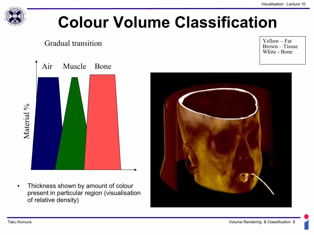
Colour Volume ClassificationM
ater
ial %
Air BoneMuscle
Gradual transition Yellow – FatBrown – TissueWhite - Bone
● Thickness shown by amount of colour present in particular region (visualisation of relative density)
Taku Komura Volume Rendering & Classification 9
Visualisation : Lecture 10
Example : Volume Rendering
Taku Komura Volume Rendering & Classification 10
Visualisation : Lecture 10
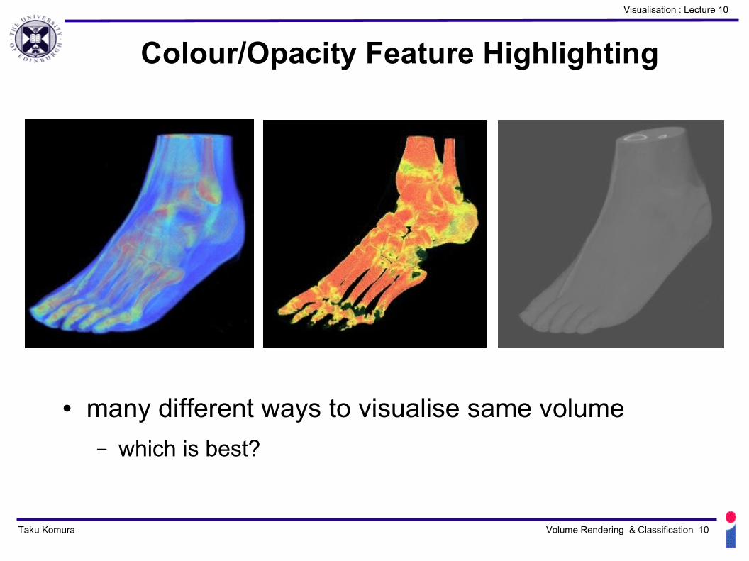
Colour/Opacity Feature Highlighting
● many different ways to visualise same volume– which is best?
Taku Komura Volume Rendering & Classification 11
Visualisation : Lecture 10
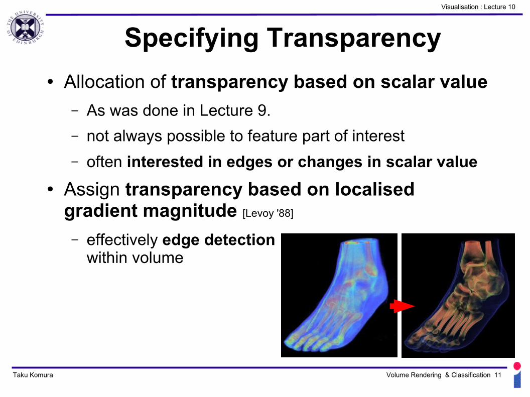
Specifying Transparency● Allocation of transparency based on scalar value
– As was done in Lecture 9. – not always possible to feature part of interest– often interested in edges or changes in scalar value
● Assign transparency based on localised gradient magnitude [Levoy '88]
– effectively edge detection within volume
Taku Komura Volume Rendering & Classification 12
Visualisation : Lecture 10
Volume Clipping● Clipping volume in X, Y, Z planes allows “slice-
though” visualisation of volumes– clip using implicit planes
Taku Komura Volume Rendering & Classification 13
Visualisation : Lecture 10
Example : carotid artery● Re-examine using volume
rendering
Taku Komura Volume Rendering & Classification 14
Visualisation : Lecture 10
Object Order Volume Rendering● process voxels in order
– back to front rendering – project each to view plane
— orthographic or perspective projection– calculate contribution to target pixel value
● As per object order rendering in CG : consider voxels as objects● How to visualize the voxels?
– Just show some blocks for the voxels?— Looks like LEGO... Doesn't look nice...
Taku Komura Volume Rendering & Classification 15
Visualisation : Lecture 10
Object Order Voxel Projection● Voxel position determined via projection
– associated target pixel is brightened
● Holes can appear in rendering due to discrete nature of pixels– zoom in closer, cell density decreases– one voxel projects to one pixel
● Solution: spread cell energy across multiple pixels - splatting
Taku Komura Volume Rendering & Classification 16
Visualisation : Lecture 10
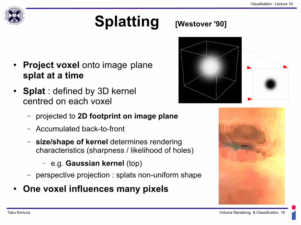
Splatting [Westover '90]
● Project voxel onto image plane splat at a time
● Splat : defined by 3D kernel centred on each voxel– projected to 2D footprint on image plane– Accumulated back-to-front– size/shape of kernel determines rendering
characteristics (sharpness / likelihood of holes)— e.g. Gaussian kernel (top)
– perspective projection : splats non-uniform shape● One voxel influences many pixels
Taku Komura Volume Rendering & Classification 17
Visualisation : Lecture 10
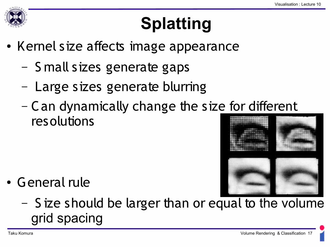
Splatting● Kernel size affects image appearance
– S mall s izes generate gaps– Large sizes generate blurring– Can dynamically change the size for different
resolutions
● General rule– S ize should be larger than or equal to the volume
– traverses both image and object space simultaneously in scan-line order
– assumes a orthographic camera model— projection perpendicular to image plane
– Fixed resolution : 1-to-1 correspondence between voxels and pixel
Taku Komura Volume Rendering & Classification 19
Visualisation : Lecture 10
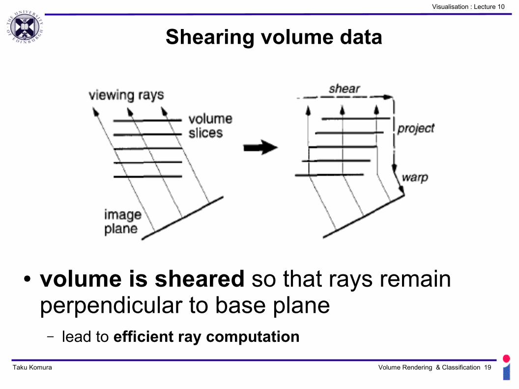
Shearing volume data
● volume is sheared so that rays remain perpendicular to base plane– lead to efficient ray computation
Taku Komura Volume Rendering & Classification 20
Visualisation : Lecture 10
Rotation of camera with shear-warpNo rotation
Small angle
Large angle
– Instead of traversing along rays, visit voxels in a plane— regardless of camera viewing angle
Taku Komura Volume Rendering & Classification 21
Visualisation : Lecture 10
Transform to sheared space
•Only one set of interpolation weights needs to be computed for all the voxels in a plane.•Remember for previous sampling, we needed to recompute the weights for every sample point!
screen
• Rays are cast from the base plane voxels at the same place.
• They intersect voxels on subsequent planes in the same location.
1 to 1
sheared volume
Taku Komura Volume Rendering & Classification 22
Visualisation : Lecture 10
Shear-warp factorisation
● Use front-to-back ordering– support early termination (last lecture)
● Both voxels and screen pixels are sampled simultaneously
● Suitable for SIMD processors (interpolating the data simultaneously for several voxels, summing vector data)
Taku Komura Volume Rendering & Classification 23
Visualisation : Lecture 10
Perspective projection
● We can also handle perspective projection● Need to shear and scale!
Taku Komura Volume Rendering & Classification 24
Visualisation : Lecture 10
Shearing factorisation from 3 different directions
● Doing the shearing for three different views (X,Y, and Z axis)
Taku Komura Volume Rendering & Classification 25
Visualisation : Lecture 10
Final stage of shear-warp● Final stage of re-sampling (warp) required
– transform resulting image from sheared space to regular Cartesian space (image plane).
View of Volume Sheared Volume
Taku Komura Volume Rendering & Classification 26
Visualisation : Lecture 10
Summary● Volume Classification
– colour / opacity transfer functions– feature extraction and highlighting
● Object Order Volume Rendering– Volume Rendering via Texture Mapping (H/W)– Shear-Warp Algorithm