Journal of Applied Economics Volume XI, Number 1, May 2008 XI Edited by the Universidad del CEMA Print ISSN 1514-0326 Online ISSN 1667-6726 Ester Faia, Massimo Giuliodori and Michele Ruta Political pressures and exchange rate stability in emerging market economies
Transcript
Journal ofAppliedEconomics
Volume XI, Number 1, May 2008XI
Edited by the Universidad del CEMA Print ISSN 1514-0326Online ISSN 1667-6726
Ester Faia, Massimo Giuliodori and Michele Ruta Political pressures and exchange rate stability in emerging market economies
POLITICAL PRESSURES AND EXCHANGE RATESTABILITY IN EMERGING MARKET ECONOMIES
ESTER FAIA
Universitat Pompeu Fabra
MASSIMO GIULIODORI
University of Amsterdam and DNB
M ICHELE RUTA ∗
European University Institute
Submitted May 2006; accepted April 2007
This paper presents a political economy model of exchange rate policy. The theory is based ona common agency approach with rational expectations. Financial and exporter lobbies exertpolitical pressures to influence the government’s choice of exchange rate policy, before shocksto the economy are realized. The model shows that political pressures affect exchange ratepolicy and create an over-commitment to exchange rate stability. This helps to rationalize theempirical evidence on fear of large currency swings that characterizes exchange rate policy ofmany emerging market economies. Moreover, the model suggests that the effects of politicalpressures on the exchange rate are lower if the quality of institutions is higher. Empiricalevidence for a large sample of emerging market economies is consistent with these findings.
JEL classification codes: F3, D7
Key words: exporters and financial lobbies, exchange rate stability
I. Introduction
Nominal exchange rates show little variation in most emerging market economies.
In a seminal article Calvo and Reinhart (2002) estimate that the probability that the
monthly variation of the nominal exchange rate is in a narrow band of plus/minus
* Michele Ruta (corresponding author): Economics Department, European University Institute,via della Piazzuola 43, 50133, Firenze, Italy. Email: [email protected]. We would like tothank Maria Bejan, Daniel Brou, Alessandra Casella, Giancarlo Corsetti, Jeffry Frieden, GiorgioDi Giorgio, Bas Jacobs, Omar Licandro, Alberto Martin, Pietro Reichlin, Jorge Streb, Rick vander Ploeg, Fabrizio Venditti and seminar participants at Columbia University, European UniversityInstitute, University of Amsterdam, LUISS and Ente Einaudi for comments and suggestions.We also thank Carmen Reinhart, Ernesto Stein and Alexander Wagner for giving us access to
JOURNAL OF APPLIED ECONOMICS2
2.5% is over 79% for countries which claim to have freely floating exchange rateregime, most of which are emerging market economies.1 For emerging economies
under managed floating regimes and with limited flexibility arrangements this
probability is respectively 87% and 92%. These numbers are surprisingly high:the same probability for pure floaters such as the United States and Japan is
respectively of 59% and 61%. This is even more remarkable considering that
emerging market economies generally experience larger and more frequent shocks.2
Furthermore, Calvo and Reinhart (2002) show that interest rate and reserve variability
are significantly higher in emerging market economies than in G3 economies,
attesting to active policies to smooth exchange rate fluctuations.One theoretical milestone in providing an explanation of exchange rate policy
for emerging market economies has been set by the models that explore the
hypothesis of liability dollarization and currency mismatch as major deterrents forexchange rate fluctuations. From an empirical point of view a recent prolific literature
has shown the importance of both liability dollarization and political and institutional
factors as main determinants of exchange rate policy (a brief survey is reported inSection II).
Our goal is to go beyond the existing literature in providing a simple model that
conjugates economic and political determinants –i.e., such as liability dollarizationand lobbying activity– and show how these elements interact to influence exchange
rate policy in emerging market economies. More precisely the model shows that
the reluctance to let the currency float is associated with pressures exerted byinterest groups representing the financial and the production sectors. This happens
even when exchange rate movements could be beneficial from a social perspective.
The stylized economic model is a one period small open economy with twogroups of individuals characterized by conflicting interests toward exchange rate
policy. The first group, which we label producers, produces a tradable good and
seeks for a loan in domestic currency in order to cover the costs of production.
their own data. Michele Ruta thanks the Leitner Program in International Political Economyat Yale University for hospitality and Ester Faia gratefully acknowledges financial supportfrom the DSGE grant of the Spanish Ministry and Unicredit-Bank Research grant. All errors areour own responsibility.
1 Calvo and Reinhart (2002) refer to this phenomenon -the deviation from the announcedfloating regime- as fear of floating.
2 For instance, volatility of real output is between two and two and half times larger in emergingmarkets than in the G7 economies.
3POLITICAL PRESSURES AND EXCHANGE RATE STABILITY
The services of this loan are chosen at the beginning of the period by the financialsector. Since producers’ revenues depend on the exchange rate while loan services
are determined in domestic currency, ex-post producers profit from exchange rate
depreciations. The second group of agents, which we label bankers, are producersof an intermediation service. They are specialized in obtaining funds from the
world market, pooling resources and supplying loans to producers in domestic
currency. The balance sheet of a typical bank is characterized by a currencymismatch since liabilities are in foreign currency while assets are in domestic
currency, therefore bankers profit from currency appreciation. As it stands, lobbies
clearly have ex-ante diverging interests concerning the direction of exchange ratemovements –e.g., appreciation for bankers and depreciation for producers–,
however and despite this they both dislike ex-post excessive volatility in the
exchange rate. The reason for this lies in the fact that foreign investors supplyfunds to intermediary by charging a premium on external finance.3 Such premium,
which is adversely affected by exchange rate volatility, increases both the cost of
liabilities for bankers and the loan services to producers. Hence the larger are theexpected movements in the exchange rate the higher are the interest rates on
domestic and foreign loans and the lower is welfare for both producers and bankers.
The political game assumes that the two sectors are politically organized –i.e.,have their interest represented by lobbies. More specifically, interest groups exert
political pressures to influence the decisions of the government in relation to the
exchange rate policy. We follow Dixit and Jensen (2003) and model this situation asa common agency game with rational expectations.4 However and contrary to their
model, we assume that the interest groups’ payoffs are (adversely) affected by the
ex-ante volatility (rather than by the expected level) of the government’s ex-postpolicy choice of the exchange rate. Political pressures take the form of incentive
schemes offered to the government at the beginning of the period –i.e., before a
shock to technology is realized. The government chooses the exchange rate policyafter the shock is observed and political pressures are exerted so as to trade-off
conflicting interests in society.
The equilibrium policy of this game is given by a weighted average of the two
3 It is plausible to assume that foreign investors bear the risk of facing informational asymmetriesand cover this cost by charging a premium for external finance.4 Dixit and Jensen (2003) extend the theory of common agency à la Bernheim and Whinston(1986) to the situation where the principals’ payoffs are affected by their ex-ante expectationof the agent’s ex-post choice. They show that the usual truthful schedule must be modified toaccount for the rational expectation constraint.
JOURNAL OF APPLIED ECONOMICS4
groups preferred policies (as in the standard common agency game à la Bernheimand Whinston 1986) and by a distortion associated with the effect on the groups’
welfare of the ex-post exchange rate volatility. This distortion results from the
attempts of organized groups to solve, in a non-cooperative way, the commitmentproblem of the government and it has the effect of limiting exchange rate movements,
thus providing a political rational for the little variation of nominal exchange rates
in emerging market economies. Each interest group attempts to influence thegovernment to enact the policy it prefers –depreciation for producers, appreciation
for bankers– but, at the same time, offers incentives to reduce expected exchange
rate volatility. Interestingly, in the political equilibrium the exchange rate does notfluctuate much even when society as a whole would find it beneficial. In other
words, lobbying activity works as an over-commitment device to exchange rate
stability: since the political pressures exerted by the two lobbies are not coordinatedthey create strong incentives for the government to stabilize the exchange rate.
The model also predicts that the exchange rate fluctuates more in countries
with better institutions (e.g. higher accountability and government effectiveness,more control of corruption, etc.) since governments are less responsive to special
interests’ political pressures.
We use ordered logit techniques to test these results for a large sample ofemerging market economies. Our measure of exchange rate stability is the de facto
exchange rate classification of Reinhart and Rogoff (2004) and Levy-Yeyati and
Sturzenegger (2005). Empirical evidence for our sample of countries supports theidea that the political influence of the production sector and of the financial sector
exposed in foreign currency is associated with more stable exchange rates, but the
less so the higher the quality of institutions.The rest of the paper is divided as follows. Section II overviews the related
literature. Section III presents the political model. In section IV we study the political
economy of exchange rate policy. Section V contains the empirical evidence.Concluding remarks follow.
II. Relation with previous literature
The recent literature has put forward several explanations for the actual behavior
of exchange rate policy in emerging markets. Liability dollarization may inducecountries to tolerate less variation in their exchange rates (see Hausmann, Panizza
and Stein 2001). Calvo and Reinhart (2002) argue that, in presence of high exchange
rate pass-through, countries that adopt inflation targeting reduce exchange rate
5POLITICAL PRESSURES AND EXCHANGE RATE STABILITY
volatility to maintain the commitment to the target. In Lahiri and Vegh (2001),
exchange rate stability arises because there is an output cost associated to exchangerate fluctuations. Alesina and Wagner (2005) suggest that fear of floating might be
used to signal high institutional quality because larger currency swings are
generally associated with fragile and weak institutions.5
Our story does not exclude some of the previous arguments but enriches them
with an important political economy dimension. First, in our model exchange rate
stability is the (equilibrium) result of a political process (i.e., lobbying activity).Therefore, differently from some of the previous works on this topic, the reluctance
to tolerate much variation in the exchange rate is not necessarily associated with
the social optimum.6 Second, we believe that previous work entails a contradictoryargument: if flexible exchange rates are associated with additional welfare costs -
due to balance sheet effects, output costs and/or credibility losses - a benevolent
social planner would not want to announce more flexibility than what it is willing todeliver. In our framework the government can announce policies which are
consistent with the social optimum, but then it deviates ex-post from the
announcements since it receives political pressures.Political economy factors have entered economic analysis long ago to answer
questions related to the allocation of public expenditure, the management of public
debt, the determination of tariffs and subsidies, etc. Few attempts have been donein the international finance literature to account for political determinants of exchange
rate policy from the theoretical point of view.7 A few exceptions are Drazen and
Eslava (2005) and Bonomo and Terra (2006), which offer theoretical models on thepolitical economy of exchange rate policy.
From an empirical point of view several analysis have been conducted to ex-
plore the importance of political factors as opposed to other economic determinants.Levy-Yeyati, Sturzenegger and Reggio (2002) conduct an empirical analysis on the
determination of exchange rates accounting for several economic and political
variables. By using a dataset for 183 countries they find that regime choices as well
5 This is in apparent contradiction with our evidence. We will come back on this point inSection V.
6 Chang and Velasco (2005) also rationalize the fear of floating as an equilibrium different fromthe social optimum. They do this in a model in which foreign denominated liabilities andexchange rate policy are determined simultaneously.
7 Frieden and Stein (2000) provide an overview of the political economy of exchange ratepolicy. Refer also to Drazen (2000), chapter 12, part 1.
JOURNAL OF APPLIED ECONOMICS6
as deviations between actual and reported policies can be well predicted by financialand political variables. Several other analysis have established the importance of
political factors in explaining exchange rate policies for emerging market economies.
Collins (1996) and Edwards (1996) use probit analysis to study the determinants ofexchange rate regimes and find that the political cost associated with devaluations
plays a key role. Finally Klein and Marion (1994) and Gavin and Perotti (1997) find
that devaluations or regime shifts are typically delayed until elections take place.In a series of papers, Frieden and Stein (2000), Frieden, Ghezzi and Stein (2001),
Blomberg, Frieden and Stein (2005) evaluate the relative importance of
macroeconomic/financial factors versus political economy elements and examinethe conflict arising for an incumbent government between inflation stabilization,
which benefits consumers, and competitiveness, which benefits producers. Among
the political economy variables an important distinction is made between thepressures exerted by interest groups on the incumbent government and electoral
considerations.
Finally it is worth mentioning that Frieden, Ghezzi and Stein (2001), Jaramillo,Steiner and Salazar (1999) and Ghezzi and Pascó-Font (2000) conduct empirical
analysis for several Latin American countries which support the motivation and
the assumptions behind our work. These authors noticed that with the advent oftrade liberalization, as specific tariffs and subsidies began to be dismantled,
producers no longer protected by trade restrictions had much stronger incentives
to lobby the government to influence exchange rate policy. Similarly, the financialsector became vocal regarding exchange rate management when restrictions on
capital flows were lifted in the 1990s. This implies that producers and the financial
sector in Latin America generally have opposing views on exchange rate policy: infavour of a competitive –i.e. depreciated– exchange rate the first group, opposed
the latter.
III. A model of common agency with rational expectations
The theory of common agency (Bernheim and Whinston 1986) has become thestandard approach to model the interaction of the government with different groups
in society (see Grossman and Helpman, 1994 and 2001). Dixit and Jensen (2003)
extend the basic common agency framework to consider the situation in which theprincipals’ payoffs are affected by their ex-ante expectations of the agent’s ex-post
choice of economic policy.
In this section we build on the Dixit and Jensen (2003) model of common
7POLITICAL PRESSURES AND EXCHANGE RATE STABILITY
agency with rational expectations and consider a different objective function ofthe principals. More specifically, we study a situation where the principals’ utility
is influenced by the level of the policy variable and the ex-ante expectations of the
policy variable volatility. In the next section we apply this model to study thepolitical economy of exchange rate policy.
The agency game has two principals, in this case two organized lobby groups,
and one agent, the incumbent government. The agent chooses a policy variable e
after the realization of a shock z. Accordingly, the government’s policy is a function
e(z). Interest groups form rational expectations on e before the shock is realized.
Let g(z) be the density function of z, we can write the conditions for rationality as
(1)
(2)
where ee and σe2 are respectively the expectation and the variance of e.
The objective functions of individuals belonging to lobby I take the general
form:
wi (e, σe2 , z), (3)
where wi can be interpreted as the (ex-post) indirect utility of a member of principali, which depends on the actual policy chosen ex-post by the government e and the
variance σe2 of e as well as on the realization of the shock z.
As a benchmark, we find first the optimal policy from the perspective of groupi. We then study the equilibrium properties of the outcome in the case of a single
lobby and for the common agency game.
A. Lobby i’ s preferred policy
The complete contingent commitment policy that principal i would most prefer isthe one that solves the following problem:
, (4)
subject to condition (2). For this optimization we construct the Lagrangian:
[ ] ∫== dzzgzezeEee )()()(
[ ] [ ][ ] dzzgzeEzezeVare )()()()( 22 ∫ −==σ
[ ]),,( max 2 zewE ei σ
JOURNAL OF APPLIED ECONOMICS8
[ ] [ ]{ })( ),,( 22 zeVarzewEL ei
ei −+= σζσ , (5)
where iζ is the Lagrange mult ipl ier on the constraint (2) and
[ ] [ ]{ } [ ]{ }22 )( )( )( zeEzeEzeVar −= . The first order conditions of this problem with
respect to e(z) and σe2 are: 8
[ ]2 ( ) ( ) 0i
iL we E e g z
e eζ
∂ ∂ = − − = ∂ ∂ (6)
022 =+
∂∂=
∂∂ i
e
i
e
wE
L ζσσ
. (7)
The last first order condition can be combined into the first one to eliminate the
Lagrange multiplier:
[ ] 0)(22=−
∂∂+
∂∂
eEew
Ee
w
e
ii
σ. (8)
This implicitly defines the optimal commitment policy from the perspective of
principal i. Notice that a change in e(z) has a direct effect on the expected value ofthe objective function of group i, as well as an indirect one by affecting the variance.
Condition (8) implies that the commitment rule preferred by principal i allows
responses to the shock z on which the government has an informational advantage.However, it also takes into account the effect on group i’s welfare of an increase in
the expected volatility of the policy variable.
B. Equilibrium policy
We now study the equilibrium properties of the lobbying game. We analyze firstthe case in which only one group is politically active and lobbies the government.
Then, we study the equilibrium of the common agency game. The policy actually
chosen is the equilibrium of a game that involves the lobby (or the two lobbies)and the government.
8 For brevity we omit the function’s arguments.
9POLITICAL PRESSURES AND EXCHANGE RATE STABILITY
The timing of the political game is as follows. At the beginning of the period,the interest group offers to the government a contract which is contingent on the
policy and the shock. If both lobbies are active, these contracts are assumed to be
offered non-cooperatively. The incentive scheme is represented by a bindingcommitment to deliver a transfer (monetary or non-monetary) to the government
when the policy is chosen. At a second stage, the shock is realized and the
government chooses the policy taking into account social welfare and theprincipal’s (or the principals’) incentive schedule(s).
This timing of events allows the government to respond to the shock but -in
the absence of a commitment technology- induces a time-consistency problem asthe government takes as given expectations on the policy variable. Lobbies, acting
under rational expectations, recognize the time-consistency problem and exert
pressure on the government to follow the rule implicit in condition (8), whichrepresents the optimal commitment policy from the perspective of lobby i. They do
so by offering a contract to the government.
Contracts offered ex-ante take the form:
(9)
This functional form of the incentive scheme assumes that group i promises to
the government a fixed payment (i.e., which depends on the shock, but not on the
policy) and a variable payment contingent on the choice of the policy variable bythe government.9 An important issue in this class of models relates to the specific
form given to the variable payment ci(e,z) in equilibrium. We come back to this
point later.The government’s objective function is given by:
, (10)
where 0 ≤ 1 − η ≤ 1 is the weight that the agent puts on the incentive schemes
T(e,z) offered by the principals, where
9 As it will be immediately clear, the choice of this functional form is mostly for analyticalconvenience: it simplifies the government participation constraint (see condition 13).
),()(),( zeczkzet iii +=
),()1(),,( 2 zeTzewwi
ei
igov ησθη −+= ∑
= ∑i
agent the tocontractsoffer principalsboth if ),(
agent theocontract t a offers principalonly if ),(),( zet
izetzeT i
i
ii
µ
µ, (11)
.
JOURNAL OF APPLIED ECONOMICS10
θi is the size of group i and µ
i is the weight that the agent puts on the contract
offered by group i.
In a model of political influence, the first and the second term in condition (10)
can respectively be interpreted as social welfare and political support by specialinterests. Accordingly, we can interpret η as a parameter that captures the quality
of the institutional system or the check-and-balances schemes limiting the ability
of interest groups to influence politicians. The parameter µi represents the political
power of group i which can be larger, smaller or equal to its economic size θi . If
economic and political influence of a group coincide, then µi = θ
i.
One lobby
We first solve the lobbying game under the assumption that only group i lobbiesthe government. In the last stage of the game, the government chooses the policy
to maximize its objective function. The first order condition for this optimization
problem is
0)1( =∂∂−+
∂∂∑ e
t
e
w i
ii
i
i µηθη . (12)
Principal i maximizes [ ]),(),,( 2 zetzewE ie
i −σ subject to several constraints.First the group recognizes that the government will set the policy according to
(12).10 Second, the contract offered by the principal needs to satisfy a government
participation constraint which reads as follows: E (wgov) ≥ w0gov
, where w
0gov
is
the utility assigned to an outside opportunity (for instance, the level of government
utility when no contract is offered). The principal recognizes that expectations will
be formed rationally. We regard the principal as if it were directly choosing thevariance of e subject to constraint (2). Consider the decision problem of group i,
the Lagrangian is
[ ]{ } [ ]{ }[ ] , ),()()1(),,(
)]([)( ),()(),,(
02i
2
2221
2
−+−+
+−−++−=
∑i
goviiie
ii
eiii
ei
i
wzeczkzewE
eEeEzeczkzewEL
µησθηλ
σλσ(13)
10 This, however, is kept implicit (as in Dixit and Jensen 2003) and in the Lagrangian belowpolicy e is assumed to be a function of the contract ti offered by group i (the only active group).
11POLITICAL PRESSURES AND EXCHANGE RATE STABILITY
whereλ1i is the Lagrange multiplier on the rationality constraint and λ
2i the multiplier
on the participation constraint of the agent. Group i’s choice variables are the
functions ki (z) and ci (z).
We can simplify the Lagrangian by noting that it depends only on the expectation
[ ])(zkE i and not directly on the function ki (z). The first order condition with
respect to this variable gives us the Lagrange multiplier on the government’s
participation constraint which reads as follows: [ ]ii µηλ )1(/12 −= . Using this, and
abstracting from the functional arguments, we can rewrite the Lagrangian of group
i as:
Consider now the effect of a change of e on this Lagrangian:
From condition (12) we have:
Using this last equation, condition (15) simplifies to:
which implies that the optimal choice of the contract that principal i offers to theagent needs to satisfy:
To interpret this condition, let’s assume that λ1i = 0. In this case condition (18)
implies that the equilibrium contract should satisfy the local truthfulness propertydefined by Bernheim and Whinston (1986).11 The present model provides a
11 For a discussion of this property see Grossman and Helpman (2001).
{ } [ ][ ]{ } . )-(1
1 )()( 0
2221
−+−−+= ∑i
govii
ie
iii wwEeEeEwEL θη
µησλ
[ ] )( )()1(
1)(21 zdezg
e
weEe
e
wdL
i
ii
i
ii
i
∂∂
−+−−
∂∂= ∑θη
µηλ
.)1( ∑ ∂∂=
∂∂−−
i
i
i
i
i e
w
e
c θηµη
[ ] )( )()(21 zdezge
ceEe
e
wdL
ii
i
i
∂∂−−−
∂∂= λ
[ ])(21 eEee
w
e
c iii
−−∂
∂=∂∂ λ
(14)
(15).
(16)
(17)
(18)
,
.
JOURNAL OF APPLIED ECONOMICS12
generalization of this property to the case in which the welfare of the principal is
affected by the ex-post volatility of the policy variable. The effect of the volatility
of the policy variable on the optimal choice for the contract offered by principal i
is captured by the last term in condition (18).
The equilibrium policy needs to be consistent with the government incentive
compatibility constraint. We therefore substitute the expression that implicitlydefines the optimal contract of principal i into condition (12):
(19)
To find an expression for the equilibrium policy, we still need the first order
condition for the choice of :2eσ
.0)1(
12122
=
∂∂
−++
∂∂=
∂∂ ∑
e
i
ii
i
i
e
i
e
i wE
wE
L
σθη
µηλ
σσ (20)
From this first order condition, we find an expression for the Lagrange multiplier
that we can substitute into (19). Rearranging, we get:
[ ] −
∂∂−−−=
∂∂−+
∂∂∑
e
i
i
i
i
i
ii
wEeEe
e
w
e
w2
)(2)1()1( ησ
µηµηθη
(21)
Condition (21) implicitly defines the equilibrium policy when only group i is
politically active. Absent lobbying, the government would set policy to maximize
ex-post social welfare (i.e., e would be such that .0)=∂
∂∑ e
wi
iiθ 12 Lobbying by
group i alters the equilibrium policy choice in two main respects. First, lobbying
induces the government to take into account the effect of policy volatility on the
[ ] .0)(2)1( 1 =
−−∂
∂−+∂
∂∑ eEee
w
e
w ii
i
i
ii λµηθη
[ ]
∂∂−−
∑i e
i
iw
EeEe2
)(2σ
θη
12 If η=1, lobbies do not offer any political contribution as this would not alter the policy choiceof the government (see condition 10).
.
13POLITICAL PRESSURES AND EXCHANGE RATE STABILITY
utility of group i when choosing policy e (see the right-hand side of condition 21).By substituting the Lagrange multiplier i1λ into condition (18), we see that the
optimal contract needs to satisfy:
(22)
which confirms that (ex-ante) lobby i optimally tailors its incentive scheme toinduce the government to internalize the effect of policy volatility on its welfare wi.
Second, and quite intuitively, the policy is biased in favor of the organized
group. This is apparent in the extreme scenario in which the government is fullynon-benevolent (i.e., η =0). In this case, from condition (21) we obtain the condition
determining the equilibrium policy:
[ ] ,0 )(22
=
∂∂−+
∂∂
e
ii wEeEe
e
w
σ (23)
which coincides with the optimal commitment policy from the perspective of group
i (see condition 8).
Two lobbies
We now solve the lobbying game under the assumption that both groups offercontracts to the common agent. In the last stage of the game, the government
chooses the policy to maximize its objective function. The first order condition is
now given by
.0)1( =∂∂−+
∂∂ ∑∑ e
t
e
w i
ii
i
ii µηθη (24)
As in the previous subsection, each principal maximizes
[ ]),(),,( 2 zetzewE ie
i −σ subject to the same set of constraints and the Lagrangian
of group i now takes the following form:13
[ ] ,)1(
)(222
∂∂
−+
∂∂−+
∂∂=
∂∂ ∑
e
i
ii
ie
iii wE
wEeEe
e
w
e
c
σθ
µηη
σ
13 Contrary to what we did for condition (13), in this case we assume that in the Lagrangian thepolicy e is a function of the contracts offered by all active groups.
JOURNAL OF APPLIED ECONOMICS14
[ ]{ } [ ]{ }[ ] , ),()()1(),,(
)]([)( ),()(),,(
02i
2
2221
2
−+−+
+−−++−=
∑ ∑i
gov
i
iiie
ii
eiii
ei
i
wzeczkzewE
eEeEzeczkzewEL
µησθηλ
σλσ
(25)
where group i takes as given the contract offered to the common agent by group
-i.It can be easily shown that under common agency the optimal choice of the
incentive scheme that principal i offers to the government needs to satisfy condition
(18).14 However, now the equilibrium policy needs to be consistent with thegovernment incentive compatibility constraint (24). We therefore substitute the
expression that implicitly defines the optimal contract of principal i and the
expression for the Lagrange multiplier i1λ into condition (24). Rearranging, we obtain
the condition that implicitly defines the equilibrium policy under common agency:
[ ] [ ] )(2)1()1(2
−
∂∂−−−=
∂∂−+ ∑∑
e
i
ii
i
i
iiw
EeEee
w
σµηµηηθ (26)
As in the case of a single lobby, the incentive schemes of the two groups
induce the government to take into account the effect of the volatility of the policyvariable on their utility. However, the dual agency game allows us to make two
additional considerations. First, let’s simplify condition (26) by assuming that the
economic and political power of each group in society coincide, i.e., iii ∀= µθ .The equilibrium policy is determined by:
[ ] [ ]2 22 ( ) 2 ( )
i i i
i ie ei i
w w wE e E e E e E e
eθ η θ
σ σ
∂ ∂ ∂ + − = − − ∂ ∂ ∂ ∑ ∑ (27)
If the left-hand side of this condition were equal to zero, the equilibrium policy
would be a weighted average of the two groups preferred policies (see equation 8).In this case we would expect the actual policy to be closer to the objective of
different groups depending on their economic weights .iθ The right hand side of
14 Clearly, this does not imply that the equilibrium contract is the same in the two cases, withone or two principals. Groups have to set their ki to satisfy the participation constraint of thegovernment, which now takes into account that both groups are offering contracts.
[ ] .)(222
∂∂−− ∑
i e
i
iw
EeEeσ
θη
15POLITICAL PRESSURES AND EXCHANGE RATE STABILITY
(27) is, however, different from zero for 0<η<1. This captures the distortion induced
on the equilibrium policy by the attempts of organized groups to solve non-
cooperatively the commitment problem of the government. This additional effect
is clearly absent in the one-lobby case.
Second, it is instructive to consider the extreme case of a fully non-benevolent
government and allow iθ to be different from iµ . For η=0 in condition (26), we
have that:
[ ] ,0)(22
=
∂∂−+
∂∂∑
e
ii
ii
wEeEe
e
w
σµ
where the equilibrium policy is a weighted average of the preferred policy of the
two groups. From this expression, it is apparent the role of political weights iµ under
common agency: the stronger the political influence of group i, the closer the
equilibrium policy is to i’s preferred policy (for given i−µ ).
IV. Political economy of exchange rate policy
In this section we apply the general framework previously described to explain
how political influence affects exchange rate policy.
Consider a one period model of a small open economy where the exchange rate
policy has different effects on the welfare of two different groups of individuals.
Population has measure one and individuals are indexed with [ ]1,0 ∈j and divided
into two groups: bankers of size [ ]1,0 ⊂Bθ and producers of size [ ]1,0 ⊂Pθ with
∑=
=BPi
i,
1θ . We label with wB the welfare of bankers and with wP the welfare of
producers.
The government adjusts the policy instrument –the nominal interest rate– to
achieve a certain target for the nominal exchange rate. To introduce the nominal
exchange rate e as a policy decision variable we assume that the money market
always clears at the prevailing exchange rate level. This is to say that either money
demand or money supply adjusts to meet the relative price –i.e., the nominal
exchange rate.
Bankers and producers’ welfare are affected by exchange rate policy. This
provides the main motivation for these groups to organize politically (i.e., form a
(28)
JOURNAL OF APPLIED ECONOMICS16
lobby) and influence the government to follow their wishes.15 In this section westudy the effects on the equilibrium exchange rate policy of political influence bybankers and producers.
As described in the previous section, political pressures take the form ofincentive contracts that groups offer to the government. One should interpret thecontract approach not only as describing remuneration to the government ormonetary bribes, but also as capturing non-monetary transfers as public honour(or criticism), career concerns of government officials, etc.
Interest groups are assumed to commit their incentive schemes to thegovernment before observing the realization of the shock to the economy. Thisassumption embeds the idea that interest groups have large influence in appointingthe government officials (e.g., the economy minister or the governor of the centralbank or a member of the board) who are in charge of managing exchange ratepolicy. Once appointed, policymakers have ex-post substantial autonomy ineconomic policy choices.
The economy has the following elements:1. The production sector produces a tradable good with technology y(z), where
z is a supply shock (to which government policy reacts). At the beginning of theperiod, producers have to seek for a loan from the home financial sector to financeproduction.
2. Firms in the financial sector lend money to producers at the beginning of theperiod. This operation will pay to the financial sector in units of domestic currency.To lend money, bankers need to acquire funds from foreign investors in foreigncurrency.
3. Bankers are exposed ex-post to the cost of exchange rate fluctuations.16
Hence we assume that there is no pass-through of the exchange rate onto the loanrate. Therefore, an unexpected depreciation (appreciation) of the exchange rate
decreases (increases) profits, and ultimately the welfare of bankers
<
∂∂
0e
w B
. 17
15 We assume that the two groups were able to solve the collective action problem of Olson(1965).
16 In practice this is so even in countries that impose tight regulations to avoid currencymismatches in bank balance sheet. Indeed in presence of an ex-post exchange rate depreciationbankers would like to transfer the cost of higher foreign funds onto interest rate loans; howeverenforcement and moral hazard problems will induce firms to refuse loan repayment.
17 This assumption can be easily rationalized in a situation in which loan contracts are preset atthe beginning of the period and cannot be changed ex-post if the government moves theexchange rate. This captures in a simple manner the idea of the currency mismatch observed inthe financial sector of several emerging market economies.
17POLITICAL PRESSURES AND EXCHANGE RATE STABILITY
Producers’ profits depend on the real exchange rate. We assume that price are
sticky (with an exogenous probability ξ firms cannot adjust prices) so that nominal
exchange rate fluctuations translate into real exchange rate fluctuations. Anunexpected depreciation (appreciation) of the exchange rate –by rising (reducing)
the competitiveness of the production sector– increases (decreases) profits, and
therefore the welfare of producers
>
∂∂
0e
wP
.
4. Foreign investors charge an external finance premium which is negativelyrelated to the volatility of the exchange rate. Microfoundations for this premium
are provided in Appendix A. Higher expected volatility of the exchange rate increases
the external finance premium and, therefore, the interest rate that the home financialsector pays to foreign investors. Bankers can shift at least part of the cost of
expected exchange rate volatility to producers.
5. The government can use ex-post exchange rate policy to redistribute wealthbetween bankers and producers. For a given expected exchange level ee, it is
socially optimal to create an unexpected depreciation (appreciation) of the exchangerate when large negative (positive) supply shocks hit the economy (i.e., e* > ee for
z low and e* < ee for z high). Here, the socially optimal exchange rate e* is the level
at which the left-hand side of condition (27) equals zero.18
6. Higher expected volatility by raising interest rates in the world market reduces
interest groups’ expected welfare
<
∂∂
02e
iwE
σ .
In sum, exchange rate policy implies a trade-off between the benefits of ex-poststabilization/redistribution and the costs of ex-ante higher expected volatility of
the exchange rate.
Under these assumptions, condition (27) implies a bias toward exchange ratestability in the sense that a politically motivated government does not allow much
exchange rate fluctuation in response to shocks that hit the economy.19 To
understand the mechanics of this result inside our model suppose that a supplyshock hits the economy in a way that the government would set e = e* > ee (refer
to Figure 1) - i.e. unexpected depreciation of the exchange rate. In this case the
18 e* is a weighted average of the exchange rate policy preferred by the two groups and theweights depend on the size of the groups.
19 As it is made clear in Section III, the dual agency game is sufficient -even if not necessarytoobtain this result (see conditions 21 and 26).
JOURNAL OF APPLIED ECONOMICS18
right-hand side of condition (27) is positive because 02
<
∂∂
e
iwE
σ . This implies
that the equilibrium exchange rate level (e′) is smaller than the one that the
government would set in the absence of lobbying (e*), even if there is still a
positive depreciation. If, instead, the shock is such that the government (absentlobbying) would create an unexpected appreciation (e = e* < ee), the right-hand
side of (27) is negative and the equilibrium exchange rate appreciation is smaller.
Figure 1. Equilibrium exchange rate policy
ee* e' e* e'
Social Welfare
ee
Under political pressures, the exchange rate tends to be de facto more stable in
response to shocks that hit the economy.
From condition (27), we can derive a less intuitive implication of the model. Onthe left-hand side of condition (27) we have the socially optimal exchange rate
policy. However, the right-hand side is different from zero and implies lower than
optimal exchange rate fluctuation. The intuition for this result is related to thestructure of the lobbying game. When deciding on political pressures, each interest
group wants to offer to the government incentives to maintain low exchange rate
variability. This is so since both groups suffer the costs of high expected exchangerate volatility. As this argument applies to both special interest groups and since
lobbies do not coordinate their political activities, the contracts offered to the
government are such that incentives to limit exchange rate volatility are too strong.As a result, the government manages the exchange rate more than what it would be
optimal from the groups’ own perspective. In other words, lobbying creates an
over-commitment to exchange rate stability.
19POLITICAL PRESSURES AND EXCHANGE RATE STABILITY
A final consideration about the model’s implications concerns the effects of
institutional quality, as captured by the parameter η , on the equilibrium policy. An
increase in η increases the cost of political influence and reduces incentives to
lobby.20 When η tends to one the government is not affected by special interests’
political pressures and sets the exchange rate policy so as to maximize ex-post
social welfare, thus fully accommodating the shock.
The model so far described has several testable implications. First, the model
suggests that the fear of currency swings observed in several emerging market
economies might be the result of the political influence exerted by different sectors
in the economy –bankers and producers– on the policymaker. However we showed
that for this to be the case we need three fundamental assumptions: a) different
sectors in the economy have an interest in the determination of exchange rate
policy; b) the intermediation sector should have liabilities denominated in foreign
currency; and c) the government lacks a commitment technology. In the next section
we test the implications of those assumptions on the volatility of the exchange
rate. Our country sample represents an interesting laboratory because these
preconditions are generally present in all emerging market economies. Furthermore
we explore the role of institutions in mitigating the bias toward exchange rate
stabilization.
V. Empirical results
In this section we test the main predictions of the theoretical model, which can be
summarized as follows: (1) tradable producers and the financial sector individually
have some influence on exchange rate policy; the larger is such influence the lower
is the exchange rate volatility that we expect (regardless of the announced exchange
rate regime) as governments –responsive to (ex-ante) political pressures– tend to
stabilize the exchange rate; (2) the joint pressure of different interest groups is also
associated with more stable de facto exchange rate regimes;21 (3) the effect induced
20 This follows directly from equation (22).
21 Notice that the theoretical model predicts that lobbying by both groups creates anovercommitment to exchange rate stability. This would be clearly difficult to prove empiricallyas it would require an exact definition of the optimal exchange rate policy. We, therefore, limitour empirical investigation to attest whether the interaction of both groups has an effect onthe de facto stability of the exchange rate in addition to the effect of individual lobbying by thetwo groups.
JOURNAL OF APPLIED ECONOMICS20
by the political pressure is mitigated when the quality of institutions is higher forboth the case of individual and joint lobbying.
To test these hypotheses we use a sample composed of Latin American and
Caribbean, and Asian countries, for which we were able to collect comparable dataon the size of the manufacturing and financial sectors. Due to the availability of
institutional quality or governance, the sample period is 1990-2000 (see Appendix
B for data sources and a description of the variables). As emphasized above,political pressures by interest groups representing the interests of tradable
producers and of the financial sector indebted in a foreign currency will induce the
government to excessively intervene in exchange rate markets. As a result, wewould expect to see a more stable de facto exchange rate (regardless of the
announced exchange rate regime) in countries where the political influence of
these groups is larger. Previous authors have looked into the impact of sectoralinterest groups on the exchange rate regime. Frieden, Ghezzi and Stein (2001)
study the political, institutional and lobbying factors determining the choice of the
exchange rate regime in Latin American countries in the period 1974-1993 findingstrong evidence in favor of the hypothesis that economies with an important
manufacturing sector are more prone to announce either floating regimes or
backward-looking crawling pegs. More recently, Blomberg, Frieden and Stein (2005)study the political determinants of the duration of exchange rate arrangements in
Latin America from 1960 to 1999. They find that the larger the tradable sector, the
less likely is the maintenance of an (announced) exchange rate regime. Lastly,Alesina and Wagner (2005) look at and find significant effects of the quality of
institutions on the choice (and renege) of the exchange rate regime in a large
sample of countries over the 1990s.Our empirical analysis is related to the aforementioned studies. In particular,
we assess the role of different lobbies –representing both the tradable and financial
sectors– on exchange rate policy (besides controlling for different degrees ofinstitutional quality or governance) and analyze a broader set of countries that
include both Latin American and Asian countries. We implement ordered logit
regressions where the dependent variable is the de facto classification of exchangerate regimes by Reinhart and Rogoff (2004) (RR hereafter). We also check our
results by repeating all regressions with the de facto classification of exchange
rate regimes by Levy-Yeyati and Sturzenegger (2005) (LYS hereafter).22 Both
22 We do not test our result using the traditional de jure classification of the exchange rateprovided by the IMF since it is not the ideal measure in our study. This is so since our model
21POLITICAL PRESSURES AND EXCHANGE RATE STABILITY
classifications (RR and LYS) share the methodology of looking at the actual or defacto, rather than announced de jure exchange rate regime. They differ, however, in
that RR classify regimes based upon a statistical analysis of the observed behavior
of actual exchange rates, whereas LYS base their index on data of official exchangerates and international reserves.23 The differences in the underlying algorithms are
reflected in a relatively low correlation coefficient of 0.31 between the two indices
within our country and period sample.Similarly to Frieden, Ghezzi and Stein (2001), as a proxy of the political influence
of tradable producers we use the percentage of the manufacturing sector in GDP
(MANUY1).24 To measure the impact of the financial sector and of its exposure toforeign currency, we build a variable by multiplying the share of the financial
sector in GDP with the percentage of total foreign denominated liabilities over
money (FINYFL1).25 Finally following Alesina and Wagner (2005), we takegovernance indicators from the studies of Kaufmann, Kraay and Zoido-Lobatón
(1999, 2002). More specifically, we use two indexes: the first is a control index for
corruption (COR), while the second is an index of composite governance (MGOV)(see Appendix B).
Our set of control variables is drawn from related works. Below we provide a
brief discussion. We control for the impact of liability denomination by using thelagged ratio of foreign liabilities to money (FLM1) and for trade openness by using
the lagged ratio of trade over GDP (OPEN1). To measure the relevance of external
shocks we use the lagged share of trade with the largest trading partner(SHTRADE1) and the volatility of the terms of trade (VOLEXT). We also include
the log of per capita GDP to control for the general level of development (LGDP),
the lagged log of inflation (LINF1) to control for the effects of inflation on exchange
provides predictions on the actual or de facto exchange rate regime rather than on the selfdeclaredone. In addition several authors (see Alesina and Wagner 2005, among others) noticed that defacto deviations of actual behavior from announcements are rather common. We would therebyexpect different implications if the de jure classification is used.
23 See Reinhart and Rogoff (2004) and Levy-Yeyati and Sturzenegger (2005) for details.
24 We implicitly assume that the sectors’ influence on policymakers is proportional to its sharein the country’s GDP. In terms of the theoretical model of the previous section this is equivalentto assume iii ∀= µθ . This is also the approach taken in Frieden, Ghezzi and Stein (2001) andBlomberg, Frieden and Stein (2005).
25 We have also tested using the share of the foreign denominated liabilities over output. Thisalternative normalization does not affect the main results.
JOURNAL OF APPLIED ECONOMICS22
rate regime and a business cycle dummy (DUMCI). Finally, we include a trendwhich could pick up the ‘climate of ideas’ regarding the appropriate exchange rate
regime in the 1990s. All regressions also include year dummies to account for other
common shocks (e.g., global financial and trade liberalization) affecting the exchangerate choice of policy makers.
Table 1 displays the regression in which the size of the two sectors and the
institutional variables are included separately. The special interests’ influence isfound to be highly significant and with a negative coefficient. This confirms the
first prediction, that countries with larger manufacturing and financial groups tend
to peg more the actual exchange rate.26 The results related to the impact of thepolitical pressure of the financial sector deserve some more comments. Indeed the
statistical significance of the proxy for the financial sector depends on the exclusion
of the total foreign denominated variable.27 This is so since this proxy, although itvaries across-countries according to the importance of the financial lobby, also
reflects the dynamics of the total foreign denominated liabilities. This creates an
identification problem and might be a potential source of multi-collinearity. We willreturn to this aspect below.
The indicator of institutional quality (MGOV) enters positively, indicating that
better institutions lead to more flexible de facto exchange rate regimes. On thispoint Alesina and Wagner (2005) find that countries that float tend to be either
very low or very high in the institutional quality scale. Our sample covers mainly
countries with relatively lower governance indices, hence our results are consistentwith their findings. Amongst the control variables, the coefficient associated with
the log of GDP per capita, which is positive and statistically significant, deserves
a comment. Alesina and Wagner (2005) find the same and give the followinginterpretation: more developed countries tend to have better institutions and
therefore opt for floating exchange rate regimes. Similarly, but more controversially,
higher (lagged) inflation rates are associated with more flexible exchange rates.28
26 Interestingly, countries with larger manufacturing sectors tend to have more flexible de jureexchange rate regimes, but in practice do not let fluctuate much the exchange rate. In fact, thedifferences of our empirical results compared to Frieden, Ghezzi and Stein (2001) do not seemto depend on the sample of countries or the period under observation, but mostly on thespecification of the dependent variable.
27 When both variables are included, FLM1 is never statistically significant, whereas the financialsector proxy FINYFL1 is negative and statistically significant only at 10% when the RRclassification is used as dependent variable.
28 In preliminary analysis we also used the average inflation rate over the previous years, whichled to similar results.
23POLITICAL PRESSURES AND EXCHANGE RATE STABILITY
The other control variables do not seem to play a strong role. Columns (3) and (4)of the same table show results for the regressions where we replaced the variable
MGOV with the control variable for the corruption index (COR). The results are
qualitatively very similar. In addition the corruption control indicator seems to bestatistically more significant. In the remaining columns of Table 1, we replicate all
the previous specifications using as dependent variable the LYS exchange rate
Table 1. Ordered logit specifications with interest groups and institutionalvariables
Notes: Robust z statistics. * significant at 10 percent; ** significant at 5 percent; *** significant at
1 percent. All regressions include year dummies. Sample period 1990-2000.
JOURNAL OF APPLIED ECONOMICS24
index. While some of the control variables loose their significance, the effects ofinterest groups and of institutional factors are qualitatively and statisticallyunaffected, indicating that our results are not sensitive to the specific de factoclassification.
Table 2 reports the specifications in which we interact the interest groupvariables with the institutional quality indicators. It is interesting to see that while
Table 2. Ordered logit specifications with interest groups interacted withinstitutions
Notes: Robust z statistics. * significant at 10 percent; ** significant at 5 percent; *** significant
at 1 percent. All regressions include year dummies. Sample period 1990-2000.
25POLITICAL PRESSURES AND EXCHANGE RATE STABILITY
countries with large manufacturing sectors tend to peg more the exchange rate,
institutional quality tends to weaken the political channel. In particular, the higher
the institutional quality or the control variable for the corruption index, the lesseffective the political pressure of the manufacturing sector is. Similar results are
found in the case of the financial sector, although higher institutional quality is
associated in this case with a smaller influence of this sector only when the LYSclassification is used as dependent variable (columns 7 and 8). This is consistent
with the idea that better institutions discourage lobbying activities, thus reducing
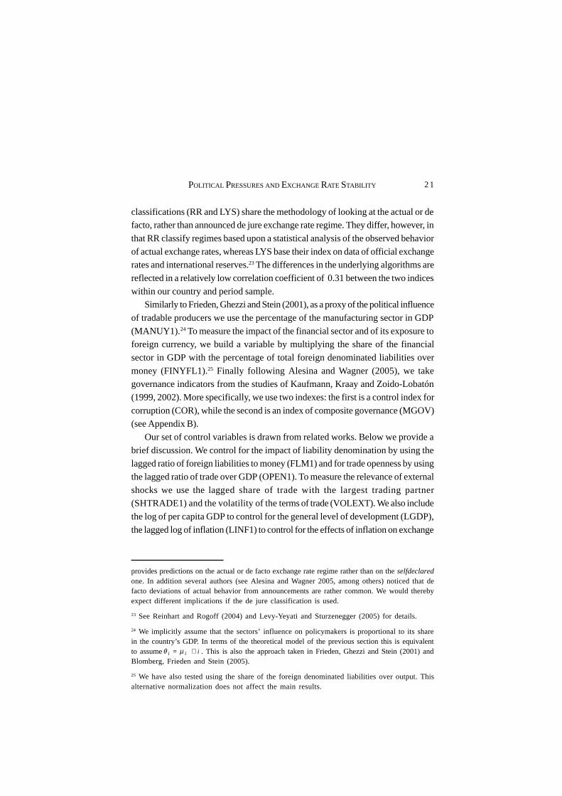
the effects of political pressures on exchange rate volatility.Finally, Table 3 reports the regressions in which we consider the joint pressure
of the manufacturing and the financial sectors by including the product of the
Table 3. Ordered logit specifications with interaction of interest groups
Notes: Robust z statistics. * significant at 10 percent; ** significant at 5 percent; *** significant
at 1 percent. All regressions include year dummies. Sample period 1990-2000.
JOURNAL OF APPLIED ECONOMICS26
share of these two variables (INTMF1). This term has the expected –i.e. negative–sign and is highly significant: consistently with the second prediction of our
theoretical model, the de facto exchange rate is more stable when the size of this
interaction term is larger. Also in this case, the LYS classification leads to verysimilar results. In columns (2) and (4) of Table 3 we also include this joint-pressure
term (INTMF1) interacted with the control for corruption index. The coefficient
associated to the latter term is negative and significant at ten percent level with theRR classification, whereas is positive and highly significant with the LYS
classification. The lack of clear-cut robust findings might be due to the high
correlation between these two variables (0.80), which makes it statistically difficultto disentangle their individual effect on the exchange rate regime.
VI. Conclusions
This paper studies the political economy of exchange rate stability in emerging
market economies. The reason for introducing political economy elements is
substantial and practical. It is substantial since economic elements do not accountalone for exchange rate policy in emerging market economies. It is practical since
several policy commentators blame the political environment for arousing the
departures of exchange rate policy from genuine principles of economic efficiency.The paper shows that the well documented fear of currency swings can be
rationalized with a common agency game under rational expectations. The key
features needed to obtain the result are as follows: a) different sectors of theeconomy (such as producers of tradable goods and bankers) have an interest in
affecting exchange rate policy, b) the presence of a currency mismatch, c) the
existence of welfare costs (for both producers and bankers) associated with expostvolatility of the exchange rate. The assumptions and implications of our model are
consistent with the empirical evidence that we report for a large set of emerging
market economies.An important theoretical dimension of our analysis is that it conjugates elements
of international finance with political factors. Besides few notable exceptions, this
type of analysis is indeed missing in the already flourishing political economyliterature which conversely has provided successful applications in several other
fields –i.e., international trade and public finance mostly. Needless to say, our
model is suitable for applications that can go beyond the scope of the specificexample. Facts concerning several historical episodes of financial crisis could
indeed be reconnected to the economic and political determinants explored in our
framework. Eichengreen and Temin (2001) for instance document the unwillingness
27POLITICAL PRESSURES AND EXCHANGE RATE STABILITY
of the Federal Reserve to abandon the Gold Exchange Standard system and linksthis to the political pressure of lobbies representing the banking sector.
Appendix
A. External finance premium
To model the emergence of an external finance premium on foreign borrowing we
use the one period debt contract by Gale and Hellwig (1985). We assume that
informational asymmetries and moral hazard affect the relation between risk neu-tral foreign lenders and the risk neutral domestic bankers. In each period there is a
continuum of competitive bankers (indexed by j) that needs to finance a continuum
of investment projects by producers, Ij. We normalize the price of those investmentprojects to 1. The producers use the funds to finance production inputs. Bankers
get funds by engaging in a financial contract with risk neutral foreign investors.
We assume the existence of an idiosyncratic shock, ωj, to the returns of eachbanker, RB. This shock can be rationalized by assuming that some bankers do not
get full repayment of the loans provided to producers. The idiosyncratic shock
has positive support, is independently distributed (across bankers) with a lognormaldistribution, F(ω), with unitary mean, and density function f(ω). The return of the
bankers is observable to the foreign investors only through the payment of a
monitoring cost µ, which is proportional to the expected return on the bankers’investment activity.
Before entering the loan contract agreement each banker owns end-of-period
internal funds for an amount NWj and seeks funds to finance producers investmentprojects, Ij. It is assumed that the required funds exceed internal funds. Hence in
every period each banker seeks funds:
eLj = I j - NWj ≥ 0. (A1)
External funds are evaluated at the prevailing nominal exchange rate, e. When
the idiosyncratic shock is above the cut-off value which determines the defaultstates, the bankers honor a repayment RL to foreign investors. On the contrary, in the
default states, the foreign investors monitor the banking activity and repossess the
assets left after the realization of the shock. Default occurs when the return to thebank ωjRBIj falls short of the amount that needs to be repaid RLeLj to foreign
investors. Hence the default space is implicitly defined as the range for ω such that:
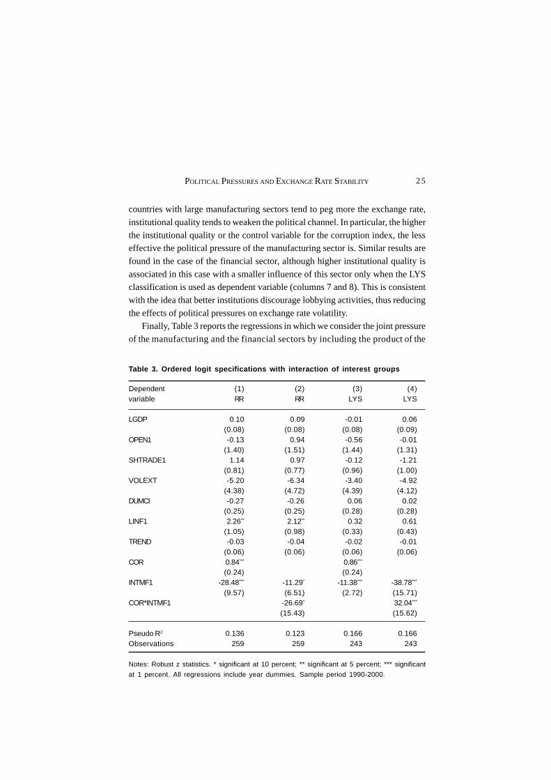
JOURNAL OF APPLIED ECONOMICS28
where ϖ j is a cutoff value for the idiosyncratic productivity shock. Let’s now
define Γ ( ϖj) and 1 − Γ ( ϖj) as the fractions of net return received by the foreign
lenders and the bankers. Hence we have:
Expected monitoring costs are defined as:
with the net share accruing to the foreign lenders being )()( jj M ϖµϖ −Γ . Foreignlenders have as outside option a risk free asset that pays a return R. The
participation constraint for the foreign lender states that the expected return from
the lending activity should not fall short of the opportunity cost of finance:
The contract specifies a pair {ϖj, Ij} which solves the following maximization
problem:
subject to the participation constraint (A5). Let χ be the Lagrange multiplier on(A5). First order conditions with respect to ωj and Ij read as follows:
Since the contract will deliver a linear relation between the external finance
premium and the leverage ration we can impose ex-ante aggregation and skip the
index j. Combining (A7) and (A8) and aggregating yields the following relationbetween the return to the bank and the risk free return:
jB
jLjj
IR
eLR≡<ϖω , (A2)
ωωϖωωωϖϖ
ϖdfdf jjj
j
∫∫∞
+≡Γ )()()(0
. (A3)
ωωωµϖµϖ
dfMj
jj )()(0∫≡ , (A4)
( ) )()()( jjjjjB NWIRMIR −≥−Γ ϖµϖ . (A5)
( ) jBj IRMax )(1 ϖΓ− , (A6)
( ))(')(')(' jjj M ϖµϖχϖ −Γ=Γ , (A7)
( ) ( )( ) χϖµϖχϖ =−Γ+Γ− )()()(1 jjjB
MR
R. (A8)
29POLITICAL PRESSURES AND EXCHANGE RATE STABILITY
RB = ρ (ϖ) R, (A9)
where
with ρ ’ (ϖ) > 0. Let’s define R
Rrp
B
≡ as the premium on external finance. By
combining (A5) with (A10) one can write a relationship between the ex-post external
finance premium, rp, and the leverage ratioNW
I:
with 0' >
− eLI
Irp . An increase in the nominal exchange rate increases loan
services and reduces bankers net worth, which in turn increases the external finance
premium.
B. Data sources and description of variables
The variables used in this article are selected from the original dataset of Alesina
and Wagner (2005). Data on the share of the sectors are collected from the
Comisión Económica para América Latina (CEPAL) for the Latin American
countries, and from the Asian Development Bank for the Asian countries. The
six institutional indicators used come from the World Bank Dataset (Kaufmann,
Kraay and Zoido-Lobatón). Assuming that these governance indices are rather
stable within the same country, we take the average of the years 1998 and 2000 and
impose the resulting value for the entire sample period 1990-2000. In our analysis
we use COR and a composite governance index MGOV constructed as a simple
average of the six indicators. The definitions of the variables used in the estimation
are in Table A1.
( )1
)()()('
))(')('))((1()(
−
−Γ+
Γ−ΓΓ−= ϖµϖ
ϖϖµϖϖϖρ M
M, (A10)
−=
eLI
Irp
R
RB
, (A11)
JOURNAL OF APPLIED ECONOMICS30
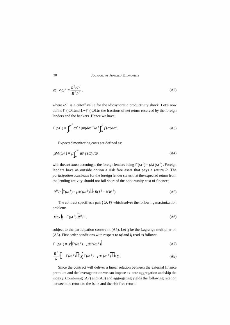
Table A1. Economic and institutional variables
Name Description
RR Reinhart-Rogoff’s de facto classification (1=peg, 5=freely falling)
LYS Levy-Yeyati and Sturzenegger de facto classification (1=peg, 4=float)
LGDP Log(GDP)
FLM1 Foreign liabilities / money, lagged
OPEN1 (Exports+imports)/GDP, lagged
SHTRADE1 Exports to the largest trading partner as share of total exports, lagged
LINF1 Log(1+inflation rate/100), lagged
VOLEXT Standard deviation of the log terms of trade over the previous 5 years
DUMCI Business cycle dummy (=1 if GDP growth in the preceding period is above
long-run growth, 0 otherwise)
MANUY1 Share of manufacturing sector over GDP, lagged
FINYFL1 Share of financial sector over GDP, lagged, multiplied by FLM1
INTMF1 MANUY1* FINYFL1
TREND Linear trend
VA Voice and accountability
PS Political stability
GE Government effectiveness
RQ Regulatory quality
RL Rule of law
COR Control of corruption
MGOV Simple average of VA, PS, GE, RQ, RL and COR
References
Alesina, Alberto, and Alexander Wagner (2005), “Choosing (and reneging on) exchange rateregimes”, Journal of the European Economic Association 4: 770-789.
Bernheim, Douglas, and Michael Whinston (1986), “Menu auctions, resource allocation, andeconomic influence”, Quarterly Journal of Economics 101: 1-31.
Blomberg, S. Brock, and Gregory Hess (1997), “Politics and exchange rate forecasts”, Journalof International Economics 43: 189-205.
Blomberg, S. Brock, Jeffry Frieden, and Ernesto Stein (2005), “Sustaining fixed rates: Thepolitical economy of currency pegs in Latin America”, Journal of Applied Economics 8:203-225.
Bonomo, Marco A., and Cristina Terra (2006), “Elections and exchange rate policy cycles”,Economics and Politics 17: 151-176.
Calvo, Guillermo, and Carmen Reinhart (2002), “Fear of floating”, Quarterly Journal ofEconomics 117: 379-408.
Cespedes, Luis Felipe, Roberto Chang, and Andrés Velasco (2004), “Balance sheets and exchangerate policy”, American Economic Review 94: 1183-1193.
31POLITICAL PRESSURES AND EXCHANGE RATE STABILITY
Chang, Roberto, and Andrés Velasco (2005), “Monetary policy and the currency denominationof debt: A tale of two equilibria” Journal of International Economics 69: 150-175.
Collins, Susan (1996), “On becoming more flexible: Exchange rate regimes in Latin Americaand the Caribbean”, Journal of Development Economics 51: 117-138.
Dixit, Avinash, and Henrik Jensen (2003), “Common agency with rational expectations:Theory and application to a monetary union”, Economic Journal 113: 539-549.
Drazen, Allan (2000), Political Economy in Macroeconomics, Princeton, NJ, PrincetonUniversity Press.
Drazen, Allan, and Marcela Eslava (2005), “Electoral manipulation via expenditure composition:Theory and evidence”, NBER Working Paper 11085.
Eichengreen, Barry (1995), “The endogeneity of exchange rate regimes”, in P. Kenen, ed.,Understating Interdependence: The Macroeconomics of Open Economy, Princeton,Princeton University Press.
Eichengreen, Barry, and Peter Temin (2001), “Counterfactual histories of the great depression”,in T. Balderston, ed., The World Economy and National Economies in the Interwar Slump,New York, NY, Palgrave Macmillan.
Edwards, Sebastian (1996), “The political economy of inflation and stabilization in developingcountries”, Economic Development and Cultural Change 42: 235-266.
Frieden Jeffry, Piero Ghezzi, and Ernesto Stein (2001), “Politics and exchange rate: A crosscountry approach to Latin America”, in J. Frieden and E. Stein, eds., The Currency Game:
Exchange Rate Politics in Latin America, Baltimore, MD, Johns Hopkins University Press.Frieden Jeffry, and Ernesto Stein (2000), “The political economy of exchange rate policy in
Latin America: An analytical overview”, Working Paper, IADB.Frieden Jeffry, and Ernesto Stein, (2001), The Currency Game: Exchange Rate Politics in Latin
America, Baltimore, Johns Hopkins University Press.Gale, Douglas, and Martin Hellwig (1985), “Incentive-compatible debt contracts: The oneperiod
problem”, Review of Economic Studies 52, 647-663.Gavin, Michael, and Roberto Perotti (1997), “Fiscal policy in Latin America”, in B.S. Bernanke
and J. Rotemberg, eds, NBER Macroeconomics Annual, Cambridge, MA, MIT Press.Ghezzi, Piero, and Alberto Pascó-Font (2000), “Exchange rates and interest groups in Peru,
1950-1996”, Working Paper, IADB.Grossman, Gene, and Elhanan Helpman (1994), “Protection for sale”, American Economic
Review 84: 833-850.Grossman, Gene, and Elhanan Helpman (2001), Special Interest Politics, Cambridge, MA, MIT
Press.Jaramillo, Juan C., Roberto Steiner, and Natalia Salazar (1999), “The political economy of
exchange rate policy in Colombia”, Working Paper, IADB.Hausmann, Ricardo, Ugo Panizza, and Ernesto Stein (2001), “Why do countries float the way
they float?”, Journal of Development Economics 66: 387-414.Kaufmann, Daniel, Aart Kraay, and Pablo Zoido-Lobatón (1999), “Governance matters”,
Working Paper, World Bank Policy Research Department.Kaufmann, Daniel, Aart Kraay, and Pablo Zoido-Lobatón (2002), “Governance Matters II:
Updated Indicators for 2000/01”, Working Paper, World Bank Policy Research Department.Klein, Michael, and Nancy Marion (1994), “Explaining the duration of exchange rate pegs”,
Journal of Development Economics 54: 387-404.Lahiri, Amartya, and Carlos Vegh (2001), “Living with the fear of floating: An optimal policy
perspective”, Working Paper 8391, NBER.
JOURNAL OF APPLIED ECONOMICS32
Levy-Yeyati, Eduardo, and Federico Sturzenegger (2005), “Classifying exchange rate regimes:Deeds vs. words”, European Economic Review 49: 1603-1635.
Levy-Yeyati, Eduardo, Federico Sturzenegger, and Iliana Reggio (2002), “On the endogeneityof exchange rate regimes”, mimeo.
Olson, Mancur (1965), The Logic of Collective Action, Cambridge, MA, Harvard UniversityPress.
Reinhart, Carmen, and Kenneth Rogoff (2004), “The modern history of exchange ratearrangements: A reinterpretation”, Quarterly Journal of Economics 119: 1-48.