1

Voyage Accounting, User Costs and the Treatment of Financial Transactions in the Theory of the Firm January 20, 2013. W. Erwin Diewert,1 Discussion Paper 13-03, Vancouver School of Economics, University of British Columbia, Vancouver, B.C., Canada, V6T 1Z1. Email: diewert@econ.ubc.ca Abstract The paper considers some of the problems associated with the indirectly measured components of financial service outputs in the System of National Accounts (SNA), termed FISIM (Financial Intermediation Services Indirectly Measured). The paper considers how to integrate financial transactions into the balance sheet and production accounts of a firm. In order to minimize the role of imputations, the paper considers a firm that raises capital at the beginning of the accounting period, engages in some form of productive activity during the period and then distributes the initial capital and any profits back to the capitalists who financed the firm. This situation corresponds roughly to merchant trading voyages made some centuries ago. Journal of Economic Literature Classification Numbers C82, D24, D92, E22, E01, E22, E31, E41, E43, E44 Keywords User costs, banking services, deposit services, loan services, production accounts, System of National Accounts, FISIM, Financial Intermediation Services Indirectly Measured, accounting theory.

1 School of Economics, the University of British Columbia, Vancouver, BC, Canada, V6T 4A9 and the School of Economics, University of New South Wales, Sydney, NSW, 2052 Australia. The author thanks William Barnett, Dennis Fixler, Robert Inklaar, Alice Nakamura, Marshall Reinsdorf, Paul Schreyer, Christina Wang and Kim Zieschang for helpful comments and the Social Science and Humanities Research Council of Canada and the Center for Applied Economic Research at the University of New South Wales for financial support. None of the above are responsible for the contents of this paper.

2

1. Introduction When we introduce financial transactions into a national income accounting framework, we encounter several problems:

• Financial transactions are by definition in nominal currency units and hence there are difficulties in determining appropriate deflators to transform these monetary transactions into real components.

• It is difficult to determine what the appropriate discount rate is for each firm in the economy. We think of the firm’s discount rate as a factor that converts transactions at the beginning of the accounting period into comparable units at the end of the accounting period.

• When user costs (and supplier benefits) are introduced into the accounting framework, the resulting user costs do not match up with the corresponding supplier benefit terms on the other side of the market, leading to a lack of additivity in the accounts (unless each firm uses the same discount rate).2

• If we try to avoid user cost imputations and just live with actual firm transactions, then we do not obtain the “right” user cost for “physical” capital services or the “right” user cost for demand deposits.

It is evident that the existing national income accounting framework does not provide a satisfactory framework for integrating firm financial transactions into the usual production accounts. In this paper, we will attempt to address some of these difficult accounting problems.3 Our approach will be to develop an accounting framework that starts out with actual firm transactions and take that approach as far as possible without introducing any extraneous imputations. In order to minimize the role of imputations, we think of an accounting period that corresponds to a fifteenth century merchant trading voyage, where at the beginning of the accounting period, the firm raises financial capital and uses the financial capital to purchase the ship and inventories of goods (this corresponds to the firm’s beginning of the period “physical” capital stock). The voyage takes place and various revenues are generated by the sale of the goods at the destination port and various costs are incurred in purchasing intermediate inputs of goods at the destination port as well as the labour inputs associated with the voyage. Further revenues are generated by the sales of the goods purchased abroad at the home port. These sales and purchases of goods and labour payments generate the firm’s cash flow or more accurately, the firm’s gross

2 See Diewert, Fixler and Zieschang (2013a) (2013b) for extensive discussions of this point. 3 Earlier work on introducing financial transactions into the system of accounts and more generally into the theory of the firm include Hancock (1985) (1991), Barnett (1987), Barnett and Hahm (1994) and Keuning (1999). For criticisms of the System of National Accounts 2008 (Eurostat, IMF, OECD, UN and the World Bank (2008)) treatment of financial sector outputs and inputs, see Hill (1996) and Sakuma (2013).

3

operating surplus.4 Finally, at the end of the return voyage, the ship is sold and the net proceeds of the voyage are distributed back to the investors in the voyage. Of course, for real life firms that undertake operations for multiple accounting periods, the accounting is more complex due to the difficulties associated with valuing the firm’s capital stocks at the end of each accounting period and so imputations for these valuations must be made. Our focus on voyage or venture accounting eliminates this extra layer of imputations. A brief outline of the paper is as follows. Section 2 develops a stylized accounting framework for a non financial firm. The model of firm behavior basically follows that of Edwards and Bell (1961) and Hicks (1961) where the accounting period is decomposed into three parts: (i) the beginning of the period; (ii) the time period between the beginning and the end of the accounting period and (iii) the end of the accounting period. At the beginning of the period, the firm raises financial capital and purchases durable inputs. In the middle of the period, the firm produces outputs and uses intermediate and labour inputs. At the end of the period, the firm sells its (depreciated) durable inputs and returns the borrowed financial capital with interest payments and returns to equity financing. Our attention in section 2 is focussed on the firm’s gross operating surplus which is equal to the value of outputs produced less intermediate and labour inputs used during the accounting period. We provide some preliminary decompositions of gross operating surplus into various payments to factors of production in this section. In section 3, we introduce the concept of a reference rate of interest, which we later specify as the average weighted cost of capital for the firm. Using the reference rate of interest and various accounting identities, we are able to decompose the firm’s gross operating surplus into more meaningful analytical terms. Two of these terms are the firm’s user cost of nonfinancial (or physical) capital and the user cost of holding demand deposits (or money). In section 4, we generalize our initial accounting framework in order to deal with the firm’s holding of very liquid assets (near money) and the granting of trade credit. We develop a model which turns out to be a version of Barnett’s (1980) Divisia monetary assets model.5 The problems associated with the deflation of financial aggregates into real components is also addressed in this section. In section 5, we consider alternative approaches to the choice of the reference rate. The two choices we consider in this section are the safe interest rate and the balancing rate of return that is often used in productivity studies. 4 Gross operating surplus less net interest payments equals cash flow. 5 Our paper is closely related to the work of Barnett (1987), who developed a model of the manufacturing firm which held monetary assets. The present paper is also related to the production theoretic models of a financial firm that were developed by Hancock (1985) (1991) and Barnett (1987). A bank is a special case of a financial firm that has the ability to create monetary deposits. The present paper does not deal with banks but using the theory in Diewert, Fixler and Zieschang (2013b) and Zieschang (2013), the reader will be able to extend the accounting framework developed in the present paper to a banking firm (just add various types of deposit accounts as an extra liability category).

4

Sections 6 and 7 consider the recently developed multiple reference rate methodologies that are due to Wang (2003) and her coauthors (section 6) and to Zieschang (2013) (section 7). Section 8 concludes with a brief summary of some of the unresolved issues associated with measuring the contribution of financial flows in production theory. 2. The Basics of Voyage Accounting We first consider the transactions that take place at the beginning of the accounting period. We assume that there are two classes of investor: one class that demands more security for their financial investments in the firm (these are the bond or debt investors)6 and a second class that is willing to take more risk (these are the equity investors). The bond investors invest the amount VB

0 at the beginning of the accounting period and expect to earn the rate of return rB

0 at the end of the accounting period. The equity investors invest the amount VE

0 and expect to earn the rate of return rE0 where rE

0 > rB0.7

Thus there is an inflow of dollars into the bank account of the firm at the beginning of the period equal to VB

0 + VE0. How are these dollars allocated? We assume that some of the

inflow dollars are held in the firm’s deposit account and denote this amount by VD0.8

Deposit accounts pay a low rate of interest equal to rD0 < rB

0 < rE0. Some of the beginning

of the period inflow dollars are invested in other securities or direct ventures. Denote the value of these investment dollars by VI

0 and these investments are expected to earn the rate of return rI

0.9 Finally, the remaining inflow dollars are allocated to the purchase of (physical) capital: we suppose that K0 units of capital are purchased at the price PK

0. We will denote the inflow of dollars less the outflow at the beginning of the accounting period by κ0. Under our assumptions, this beginning of the period net inflow of dollars10 is equal to 0; i.e., we have:11 (1) κ0 ≡ VB

0 + VE0 − PK

0K0 − VD0 − VI

0 = 0.

6 These investors could be households, other nonfinancial firms or banks. The various asset classes should be regarded as vectors but in order to simplify the notation, we will consider only a highly aggregated situation with a single representative asset in each asset class. 7 The difference in these expected rates of return is regarded as a risk premium. Later, we will note that it is possible to regard rB

0 and rE0 as ex post rates of return rather than expected rates of return.

8 For simplicity, we assume that these deposits are held to the end of the accounting period. The analysis needs to be extended to include asset and inventory transactions that take place within the accounting period. The analysis in Diewert (2005a) which dealt with the integration of nonfinancial inventory transactions could be extended to the present framework. 9 These investments could be direct equity investments in subsidiaries or financial investments in stocks and bonds that are purchased in various markets. If we were considering a banking firm instead of a nonbanking firm, the investment category would be decomposed into loans of various types, holdings of liquid assets that are driven by regulatory constraints and other real investments. 10 Note that κ0 can be interpreted as a kind of beginning of the period cash flow. 11 The student of accounting will recognize that we are essentially taking a double entry bookkeeping approach to the transactions of the firm, except that all of the transactions that take place between the beginning and the end of the accounting period are deferred until the end of the accounting period.

5

Note that κ0 is also equal to the beginning of the period value of liabilities, VB

0 + VE0,

less the beginning of the period value of assets, PK0K0 + VD

0 + VI0. Note also that

investments in real assets, PK0K0, can be decomposed into price and quantity components

but the other financial categories have no natural deflators associated with them. At the end of the accounting period, the firm will have accumulated the Gross Operating Surplus GOS1. This is equal to the value of revenues generated by the firm during the accounting period, less the value of intermediate inputs less the value of labour service payments.12 Since there are no major accounting difficulties with the components of Gross Operating Surplus, we will not provide a detailed breakdown of these components. We will now consider the (expected) inflows and outflows of dollars at the end of the accounting period.13 GOS1 is the first component of the inflows. The second component, PK

1(1−δ)K0, is the value of the sale of the depreciated capital stock, where PK1 is the end

of period price of a new unit of the capital stock and δ is the depreciation rate. The third component, VD

0(1+rD0), is the value of the firm’s initial stock of deposits, VD

0, plus the interest paid by the bank on these deposits, rD

0VD0. The fourth component, VI

0(1+rI0), is

the value of the firm’s investments in other financial assets, VI0, (this term is the return of

the capital invested at the beginning of the period) plus the expected return earned on these investments, rI

0VI0. The fifth component is the return of the capital borrowed from

bond holders plus the interest earned by these debt investors, −VB0(1+rB

0). This item is a cash outlay and so it has a negative sign in front of it. The sixth component is the return of the capital borrowed from equity providers of funds plus the (expected) waiting and risk assumption services earned by these equity investors, −VE

0(1+rE0). This item is also a

cash outlay14 and so it has a negative sign in front of it. Finally, after all the above outflows are subtracted from the above inflows, the firm may earn a pure profit at the end of the period. This end of period expected pure profit π1 is defined as the above expected cash inflows less the above expected cash outflows: (2) π1 ≡ GOS1 + PK

1(1−δ)K0 + VD0(1+rD

0) + VI0(1+rI

0) − VB0(1+rB

0) − VE0(1+rE

0). We will now take an end of period or ex post perspective and assume that we are at the end of the accounting period and GOS1, PK

1, δ, and of the rates of return which appear in (2) are known.15 If π1 is positive, then the firm makes a profit on its operations for the accounting period and this pure profit will be distributed back to the equity owners as a premium to their expected rate of return rE

0. If π1 is negative, then the equity owners will

12 Note that we are assuming that all of the flow transactions within the accounting period are realized at the end of each period. This is consistent with traditional accounting treatments of assets at the beginning and end of the accounting period and cash flows that occur during the period; see Peasnell (1981; 56). Note also that the transactions that are aggregated into GOS have natural price and quantity components. 13 For simplicity, we are neglecting tax complications. 14 The interest part of this outlay is an imputed outlay; i.e., it is necessary to have an estimated cost of equity financing in order to compute this outlay. 15 It will be difficult to determine the required rate of return on equity capital, rE

0.

6

not make their “required” ex ante rate of return and the ex post actual rate of return can be obtained by setting π1 equal to 0 and solving for the resulting rE. In principle, all of the transactions that are listed on the right hand sides of (1) and (2) have counterparts in the rest of the economy and so if we kept track of all financing decisions, interest flows in addition to the usual input and output flows in the production accounts of a system of national accounts, we could construct an expanded set of production accounts that included financial transactions which would add up; i.e., every transaction for a single sector in the expanded accounts would show up as a transaction in another sector of the accounts. There would be no lack of additivity problem in such a set of expanded accounts. The problem with such a set of accounts is that the transactions on the right hand side of (2) look rather unfamiliar! Thus in what follows, we will attempt to transform (2) into a more familiar set of transactions. In particular, we would like the user cost of nonfinancial capital to show up on the right hand side of (2). Since the beginning of the period value of liabilities equals the corresponding value of assets (recall equation (1) above), we can add the net value of liabilities from the right hand side of (1) and we obtain the resulting expression for π1: (3) π1 = GOS1 − δPK

1K0 + (PK1 − PK

0)K0 + rD0VD

0 + rI0VI

0 − rB0VB

0 − rE0VE

0. Now equation (3) can be reorganized to give us a decomposition of the firm’s gross operating surplus in terms of pure profits π1 and the other terms on the right hand side of (3): (4) GOS1 = π1 + [δPK

1 − (PK1 − PK

0)]K0 − rD0VD

0 − rI0VI

0 + rB0VB

0 + rE0VE

0. The terms in square brackets on the right hand side of (4) can be recognized as part of the user cost of capital services except that the imputed interest rate term is missing; i.e., δPK

1 is the depreciation term and − (PK1 − PK

0) is the revaluation term in the usual user cost of capital. However, the remaining terms on the right hand side of (4) look unfamiliar. But it is true that the right hand side of (4) gives us an explicit decomposition of the gross operating surplus of the firm into explanatory factors where the financing decisions of the firm figure prominently in this decomposition.16 3. The Reference Rate and Analytic Decompositions of Gross Operating Surplus 16 If we simplify the accounts by absorbing the pure profits term into the ex post return on equity (i.e., set π1 = 0 and use equation (2) or (3) to solve for the balancing rate of return on equity that makes the equation equal to zero), then all of the terms on the right hand side of (4) will have offsetting entries elsewhere in an expanded set of accounts. When we subtract depreciation from gross operating surplus, we obtain net operating surplus. The placement of the revaluation term is more controversial; if the price of the asset declines over time due to technical progress, then the revaluation term could be regarded as an obsolescence charge and could be added to wear and tear depreciation. However, if the price of the asset increases over time, then the revaluation term typically shows up in the revaluation accounts of the System of National Accounts. But the basic point here is that there is no additivity problem in principle with the expanded system of accounts when we use the decomposition of gross operating surplus given by (4).

7

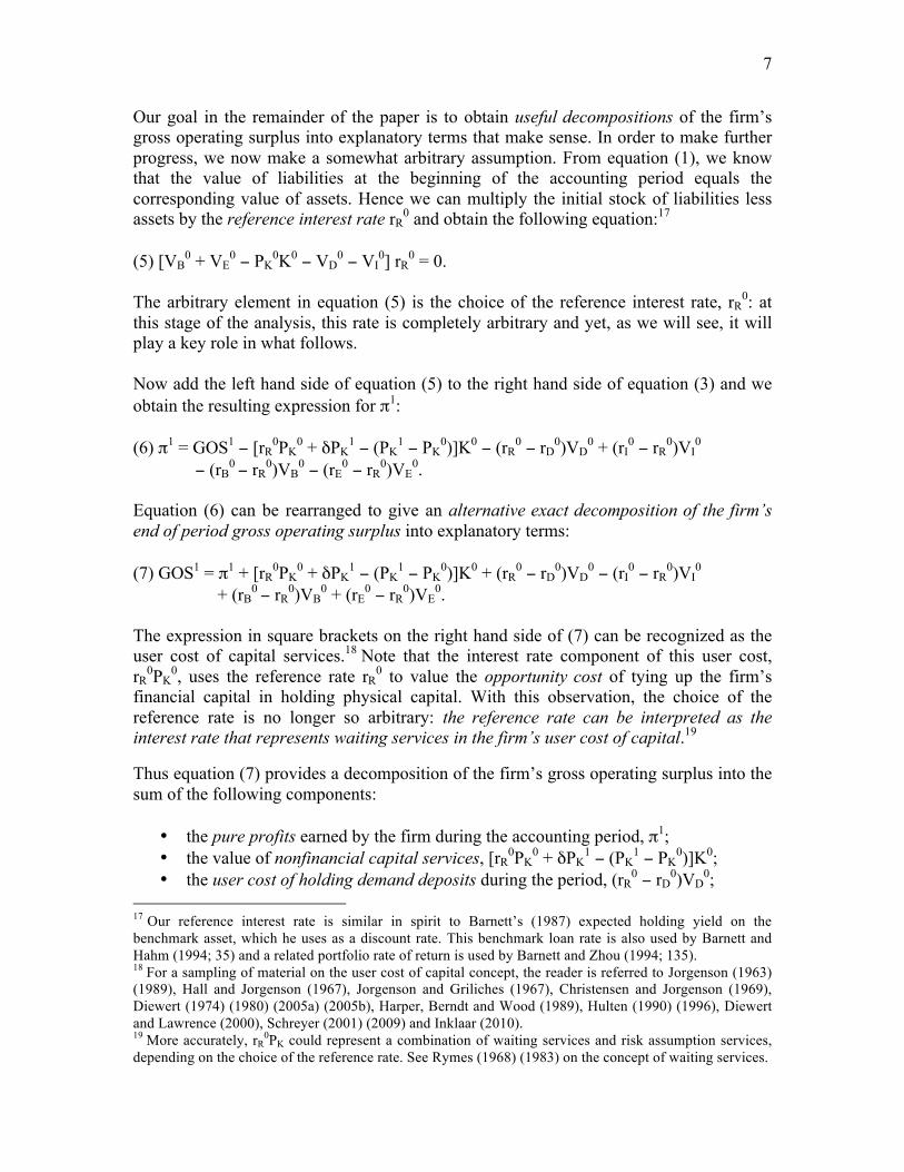
Our goal in the remainder of the paper is to obtain useful decompositions of the firm’s gross operating surplus into explanatory terms that make sense. In order to make further progress, we now make a somewhat arbitrary assumption. From equation (1), we know that the value of liabilities at the beginning of the accounting period equals the corresponding value of assets. Hence we can multiply the initial stock of liabilities less assets by the reference interest rate rR

0 and obtain the following equation:17 (5) [VB

0 + VE0 − PK

0K0 − VD0 − VI

0] rR0 = 0.

The arbitrary element in equation (5) is the choice of the reference interest rate, rR

0: at this stage of the analysis, this rate is completely arbitrary and yet, as we will see, it will play a key role in what follows. Now add the left hand side of equation (5) to the right hand side of equation (3) and we obtain the resulting expression for π1: (6) π1 = GOS1 − [rR

0PK0 + δPK

1 − (PK1 − PK

0)]K0 − (rR0 − rD

0)VD0 + (rI

0 − rR0)VI

0 − (rB

0 − rR0)VB

0 − (rE0 − rR

0)VE0.

Equation (6) can be rearranged to give an alternative exact decomposition of the firm’s end of period gross operating surplus into explanatory terms: (7) GOS1 = π1 + [rR

0PK0 + δPK

1 − (PK1 − PK

0)]K0 + (rR0 − rD

0)VD0 − (rI

0 − rR0)VI

0 + (rB

0 − rR0)VB

0 + (rE0 − rR

0)VE0.

The expression in square brackets on the right hand side of (7) can be recognized as the user cost of capital services.18 Note that the interest rate component of this user cost, rR

0PK0, uses the reference rate rR

0 to value the opportunity cost of tying up the firm’s financial capital in holding physical capital. With this observation, the choice of the reference rate is no longer so arbitrary: the reference rate can be interpreted as the interest rate that represents waiting services in the firm’s user cost of capital.19 Thus equation (7) provides a decomposition of the firm’s gross operating surplus into the sum of the following components:

• the pure profits earned by the firm during the accounting period, π1; • the value of nonfinancial capital services, [rR

0PK0 + δPK

1 − (PK1 − PK

0)]K0; • the user cost of holding demand deposits during the period, (rR

0 − rD0)VD

0; 17 Our reference interest rate is similar in spirit to Barnett’s (1987) expected holding yield on the benchmark asset, which he uses as a discount rate. This benchmark loan rate is also used by Barnett and Hahm (1994; 35) and a related portfolio rate of return is used by Barnett and Zhou (1994; 135). 18 For a sampling of material on the user cost of capital concept, the reader is referred to Jorgenson (1963) (1989), Hall and Jorgenson (1967), Jorgenson and Griliches (1967), Christensen and Jorgenson (1969), Diewert (1974) (1980) (2005a) (2005b), Harper, Berndt and Wood (1989), Hulten (1990) (1996), Diewert and Lawrence (2000), Schreyer (2001) (2009) and Inklaar (2010). 19 More accurately, rR

0PK could represent a combination of waiting services and risk assumption services, depending on the choice of the reference rate. See Rymes (1968) (1983) on the concept of waiting services.

8

• (less) the net margins earned by the firm on its financial investments, − (rI0 −

rR0)VI

0 (this is the firm counterpart to loan margins earned by banks on their loan portfolios) and

• the sum of two terms, (rB0 − rR

0)VB0 + (rE

0 − rR0)VE

0, which reflect the relative costs of raising financial capital via debt and equity capital, rB

0VB0 + rE

0VE0,

relative to raising the same amount of financial capital at the reference rate, rR

0VB0 + rR

0VE0.

Typically, the reference rate rR

0 will lie between the debt interest rate rB0 and the required

equity rate of return rE0.20 Under these conditions, (rB

0 − rR0)VB

0 will be negative and (rE0

− rR0)VE

0 will be positive. Thus the positive term (rE0 − rR

0) can be interpreted as a positive equity premium that is earned by equity capital for taking on more risk and the negative term (rB

0 − rR0) can be interpreted as a negative debt discount to reflect the lower

risk that is associated with the provision of debt capital. Alternatively, rE0 − rR

0 can be interpreted as the user cost of raising financial capital via equity financing, relative to the average cost of raising funds and since rB

0 − rR0 = − (rR

0 − rB0), rR

0 − rB0 can be interpreted

as the supplier benefit 21 to the firm of raising financial capital via debt financing. A natural choice for the reference rate is rC

*, the weighted average cost of raising financial capital from debt and equity financing;22 i.e., define rC

* as follows: (8) rC

* ≡ [rB0VB

0 + rE0VE

0]/[VB0 + VE

0]. Replacing the general reference rate rR

0 in (7) by rC* leads to the following decomposition

of gross operating surplus: (9) GOS1 = π1 + [rC

*PK0 + δPK

1 − (PK1 − PK

0)]K0 + (rC* − rD

0)VD0 − (rI

0 − rC*)VI

0. Thus the last two terms on the right hand side of (7) have vanished on the right hand side of (9)23 and so when we set the reference rate equal to the firm’s average cost of financial funds, we find that gross operating surplus is equal to pure profits π1, plus the value of nonfinancial capital services [rC

*PK0 + δPK

1 − (PK1 − PK

0)]K0 plus the cost of deposit services (rC

* − rD0)VD

0 less margins on financial investments and loans − (rI0 − rC

*)VI0.

20 Firms are generally able to raise financial capital at a lower average cost if they offer investors different degrees of risk on their investments. Thus the weighted average cost of capital will usually lie between the lower cost of debt capital and the higher cost of equity capital. 21 See Diewert, Fixler and Zieschang (2013a) for the introduction of the term “supplier benefit” as a term for a negative user cost. 22 Inklaar (2010) used this reference rate in his study of U.S. productivity. His study used a methodology that is similar to ours except he focused on adding various intangible assets to his asset base rather than adding monetary assets to the nonreproducible asset base. 23 Of course, these two missing terms (which sum to zero when the reference rate is defined by (8)) can be brought back onto the right hand side of (9) if this is desired for some analytic purpose but the decomposition given by (9) seems to be very suitable for production function studies of the firm. In particular, if the firm held no monetary deposits and made no outside financial investments, our model that uses the average cost of raising financial capital as the reference rate collapses down to a traditional user cost model for a nonfinancial firm.

9

This seems to be a satisfactory analytical decomposition of gross operating surplus for a non banking firm.24 However, other choices for the reference rate are possible as we shall see in the next two sections. The question of where to place the last two terms on the right hand side of (9), (rC

* − rD

0)VD0 − (rI

0 − rC*)VI

0, in a national income accounting framework now arises; i.e., should these terms be moved out of the income side of the accounts into the production accounts (the output and intermediate input part of the accounts)? The first term is the imputed value of deposit services and the second term is the negative of loan and investment margins times the value of investments. Since deposit services provided by banks are regarded as an output in the SNA, consistency with the SNA approach implies that the first term should be moved out of the income accounts and into the intermediate input part of the accounts. Similarly, since bank loan services are generally regarded as a banking sector output, consistency across sectors would suggest that the last term be moved into the output part of the accounts. This is a sensible strategy but it would be useful to distinguish these new rows of the production accounts as financial outputs and inputs that require special treatment. The special nature of these financial transactions is due to the following factors:

• There are no natural deflators for the entries in these financial rows25 and so users need to be alerted to the fact that the corresponding real or volume entries will necessarily be somewhat arbitrary.

• We cannot expect these entries for a specific firm or sector to be offset by another entry in the accounts that is equal in magnitude but opposite in sign to the entries in these financial outputs and inputs due to the fact that reference rates will generally be different across sectors; i.e., additivity will in general be lost for the rows in the production accounts that correspond to these financial outputs and inputs.26

In the following section, we will extend the above model by decomposing the value of firm financial investments, VI, into two components: one component which has a low rate of return associated with it and another which has a higher rate of return. 4. Barnett’s Monetary Aggregates and the Deflation Problem Barnett (1980) worked out a nice theory of monetary aggregation that applied to households.27 He noted that very liquid assets could serve as a fairly close substitute for deposits and hence broader measures of monetary holdings could be derived by applying 24 There is a similar decomposition for a banking firm but we must add an extra set of terms due to the fact that a bank can create deposits; see Diewert, Fixler and Zieschang (2013b) for the details. 25 More detailed modeling of the firm would probably lead to more definite choices for deflators for financial transactions. Barnett, Fisher and Serletis (1992; 2093) have a nice review of the contributions of Feenstra (1986) and Fischer (1974) and others to obtain deflators for the monetary holdings of households and firms in the context of more detailed models. 26 See Diewert, Fixler and Zieschang (2013a) (2013b) for an elaboration of this point. If the reference rate is chosen to be the same across all sectors in the system of accounts, then additivity can be restored. 27 He later extended his theory to cover banks and “manufacturing firms”; see Barnett (1987).

10

modern index number theory and forming broader monetary aggregates. To apply his framework in our present firm context, we need to decompose the firm’s holdings of financial investments, VI

0, into at least two components:28

• Holdings VIL0 of a very liquid asset that earns the low interest rate rIL

0 which is less than the reference rate rR

0 and • Holdings VIH

0 of a risky asset that earns the high interest rate rIH0 which is greater

than the reference rate rR0.

The very liquid assets VIL

0 can be regarded as part of the firm’s working capital, along with its holdings of demand deposits, VD

0. Using the decomposition of VI

0 into VIL0 plus VIH

0, equations (3), (5) and (7) become the following equations: (10) π1 = GOS1 − δPK

1K0 + (PK1−PK

0)K0 + rD0VD

0 + rIL0VIL

0 + rIH0VIH

0 − rB0VB

0 − rE0VE

0 ; (11) [VB

0 + VE0 − PK

0K0 − VD0 − VIL

0 − VIH0]rR

0 = 0 ; (12) GOS1 = π1 + [rR

0PK0 + δPK

1 − (PK1 − PK

0)]K0 + (rR0 − rD

0)VD0 + (rR

0 − rIL0)VIL

0 − (rIH

0 − rR0)VIH

0 + (rB0 − rR

0)VB0 + (rE

0 − rR0)VE

0. Equation (12) is the new decomposition of gross operating surplus into analytical components. Under our assumptions on interest rates, the terms (rR

0 − rD0)VD

0 and (rR0 −

rIL0)VIL

0 will both be positive and it is evident that these terms represent the opportunity costs (relative to the cost of capital rR

0) of holding the amount VD0 in demand deposits

and the amount VIL0 in low yielding, liquid investments throughout the period. The two

terms are in nominal dollar units and in order to apply index number theory to these two components of broadly defined monetary services, we need to decompose these two value flows into price and quantity components. Let ρD

0 and ρIL0 be appropriate deflators

for these two value flows. Then the prices and quantities of the two components of monetary services are defined as follows: (13) PD

0 ≡ (rR0 − rD

0)ρD0 ; PIL

0 ≡ (rR0 − rIL

0)ρIL0 ; QD

0 ≡ VD0/ρD

0 ; QIL0 ≡ VIL

0/ρIL0 .

Barnett (1980; 17) (1987) used the same true cost of living index (or alternatively, a consumer price index could be used) to deflate all of his household nominal monetary variables into real variables. In our firm context, it is not so clear what the appropriate deflators, ρD

0 and ρIL0, should be. We will discuss this choice problem below. Given the

prices and quantities of monetary assets defined by (13), we can follow Barnett (1980; 39) and use a superlative index number formula to construct a monetary aggregate for the two assets.29 28 Of course, VI

0 can be further decomposed into many assets, including accounts receivable (or trade credit). 29 See Diewert (1976) for the definition of a superlative index. Barnett (1980; 39) for his household example used the Fisher and Törnqvist superlative indexes and found that the two formula gave identical results to three decimals and commented that “the choice between these two indices is of no importance”.

11

How should the asset deflators ρD0 and ρIL

0 be chosen? There is no unambiguous answer to this question. If average stocks of monetary balances are being held in order to make payments to variable inputs and to fund purchases of inventory stocks and other capital input purchases, then a price index ρX

0 for the value of (expected) input purchases during the period would be an appropriate deflator for the firm’s holdings of deposits and other near monetary stocks. What deflator should be used to deflate the firm’s high yielding investments, VIH

0? One could argue that the real cost of making these investments is the fact that money spent on risky investments cannot be spent on input purchases and hence the same input price index ρX

0 could be used as a deflator for these risky investments. Another alternative would be to deflate all financial nominal amounts by a suitable consumer price index ρC

0. The justification for this alternative would be to measure the real value of a monetary unit in terms of a representative consumption bundle or more generally, in terms of a cost of living index for a reference population.30 Obviously, the above paragraph on deflation of monetary flows is very incomplete. Basu (2009) summed up the unsatisfactory treatment of financial variables in economic theory as follows: “No method of measuring financial sector prices (and hence real output) has yet commanded a consensus. In fact, there is even disagreement about how to measure nominal output in one of the most important financial sectors, namely banking. Thus, it is not surprising that I shall propose different answers than Fixler to the questions that he raises. But more important than the specifics of any particular issue is a general contention: in economics, when a conceptual disagreement has lasted a long time with no resolution in sight, it is usually a sign that economic theory has not been applied sufficiently rigorously. The only way to make progress in this area is to start from detailed models of what financial institutions actually do, and the market environment in which they operate. Once that is done, the measurement implications are usually obvious in principle, although the implied measures may be exceedingly difficult to implement in practice.” Susanto Basu (2009; 267). We conclude this section with a further cautionary note: we have not modeled the riskiness of alternative financial investments in a completely rigorous way.31 However, until the theory of firm behaviour under uncertainty with explicit modeling of the firm’s financing decisions has been developed to the extent that there is an accepted consensus on how to proceed, we will have to make do with incomplete modeling. Since there is an urgent need to develop an adequate accounting framework for measuring financial outputs and inputs in a national income accounting framework, we hope that the approaches explored in this paper will be useful in forming a consensus on how to proceed at a practical level. In the following sections of this paper, we revert back to the more aggregated model of firm behavior that was described in sections 2 and 3 above. The subsequent discussion

30 Feenstra (1986) and Barnett (1987) use a consumer price index as the deflator in their work (as do many others). 31 See Wang (2003), Barnett and Zhou (1994), Barnett and Wu (2005) and Wang, Basu and Fernald (2009) for rigorous approaches to the treatment of uncertainty in a user cost context. However, a consensus on the “right’ approach to the treatment of uncertainty in a national income accounting framework has not yet emerged.

12

will focus on alternative choices for the reference rate and on generalizations of the model in section 3 to include multiple reference rates. 5. Alternative Choices for the Reference Rate There are advantages in assuming that there is only a single reference rate rR

0 for the firm, since this assumption leads to a useful interpretation for the firm’s end of the period profits. Using definitions (1) and (2) (which essentially define the cash inflows and outflows of the firm at the beginning and end of the period) and the assumption (5) of a single reference rate, it be seen that the firm’s end of period profits can be written as follows: (14) End of period profits = κ0(1+rR

0) + π1. Thus if the firm chooses inputs and outputs to maximize the right hand side of (14), this will be equivalent to the maximization of discounted cash flows; i.e., (14) is equivalent to the maximization of κ0 + (1+rR

0)−1π1. The maximization of discounted cash flows is the traditional approach to intertemporal production theory.32 In section 3, we considered the implications of choosing the reference rate equal to the average cost of raising debt and equity financial capital. Another possible choice is the safe interest rate, rS

*. This rate would correspond to the yield on triple A rated assets or on bond rates for short term government securities (for a country with a suitably high debt rating). Inserting this choice of reference rate into (7) leads to the following decomposition of the firm’s gross operating surplus: (15) GOS1 = π1 + [rS

*PK0 + δPK

1 − (PK1 − PK

0)]K0 + (rS* − rD

0)VD0 − (rI

0 − rS*)VI

0 + (rB

0 − rS*)VB

0 + (rE0 − rS

*)VE0.

Comparing the decomposition given by (15) with our earlier decomposition (9) which used the cost of funds reference rate rC

*, it can be seen that we now have an extra two terms, namely (rB

0 − rS*)VB

0 and (rE0 − rS

*)VE0. Both of these terms will generally be

positive since the safe rate of return will generally be below the bond and equity interest rates. The question is: what should we do with these two terms? Should they be left in the income part of the accounts or should they be shifted into the production accounts where they would appear as sectoral intermediate input costs. The latter treatment seems to be a logical one if we have shifted loan and investment margins into the production accounts since the last two terms in (15) are similar in nature (but of course, they will generally have the opposite sign to loan margins). The major advantage of choosing the reference rate to be the safe interest rate is that the various margins and user costs on the right hand side of (15) will have offsetting entries in other parts of the system of national accounts

32 See Hicks (1939). See Edwards and Bell (1961), Hicks (1961), Diewert (1980) (2010; 760-762) and Diewert, Fixler and Zieschang (2013b) for the specialization of this theory to the case of a single period. Diewert (2010; 760) called this the Neo-Austrian approach to producer theory and noted that by recognizing goods in process, a general intertemporal production model can be reduced to a sequence of one period problems. This approach to intertemporal production theory is due to Böhm-Bawerk (1891).

13

so that additivity of the system can be preserved. However, a possible disadvantage of the choice of the safe rate as the reference rate is that as compared with the choice of the cost of funds rate rC

* as the reference rate, the value of capital services and of deposit services will be dramatically reduced and the value of loan and investment margin services, (rI

0 − rS

*)VI0, will be dramatically increased. Finally, the user costs of raising funds via debt

and equity relative to raising funds at the safe interest rate, (rB0 − rS

*)VB0 and (rE

0 − rS

*)VE0 respectively, will both become large and positive. These last two margins become

large and positive at the cost of the capital services term becoming smaller and this is the difficulty with the use of the safe interest rate as the reference rate. Essentially, these last two terms can be interpreted as extra profits that the firm has to earn in order to cover its costs of raising financial capital. Thus we have shifted costs out of the user cost of capital and into these margin terms which seems to be a dubious strategy. Another alternative strategy that is frequently used in order to determine the reference rate for a nonfinancial firm is to use the balancing rate of return reference rate rBR

*, which is defined by assuming that π1 = 0 and by solving the following equation which sets the user cost of capital times K0 equal to the gross operating surplus: (16) GOS1 = [rBR

*PK0 + δPK

1 − (PK1 − PK

0)]K0 or (17) rBR

* ≡ {GOS1 – [δPK1 − (PK

1 − PK0)]K0}/PK

0K0. Thus all of the financial transactions of the firm are suppressed in the decomposition of gross operating surplus that is given by (16). Now we want to compare the balancing rate of return rBR

* with the cost of funds rate of return rC* defined by (8). When we set π1 = 0,

the cost of funds decomposition of gross operating surplus defined by (9) can be rewritten as follows: (18) GOS1 – [δPK

1 − (PK1 − PK

0)]K0] = (rC* − rD

0)VD0 + (rC

* − rI0)VI

0. Using (17) and (18), it can be seen that we have the following relationship between rBR

* and rC

*: (19) rBR

* = [(rC* − rD

0)VD0 + (rC

* − rI0)VI

0]/PK0K0.

Usually, a nonfinancial firm will hold demand deposits and since the deposit rate rD

0 will almost always be well below the firm’s average cost of capital rC

*, it can be seen that the first term on the right hand side of (18) will generally be positive. A nonfinancial firm will typically not have substantial financial investments and if it does, usually the rate of return earned on these financial investments rI

0 will be close to the firm’s cost of capital rC

*. Thus typically, the right hand side of (18) will be positive and so the balancing rate of return will generally exceed the firm’s cost of raising financial capital; i.e., typically (20) rBR

* > rC*.

14

Thus relative to the more accurate decomposition of gross operating surplus that is given by (9), the less accurate decomposition given by the usual balancing rate of return methodology (17) will have the following characteristics:

• The value of nonfinancial capital services will generally be overstated; • The value of deposit services will be dramatically understated (since they will

normally be set equal to zero33) and • The role of investment or loan margins will be missing.

The fact that deposit services are missing in traditional production function studies of the economy that use the balancing rate of return methodology is potentially large source of bias in these studies, since presently, many firms in developed economies are holding very large deposit balances. 6. Multiple Reference Rate Methodologies: The Wang Group Approach Rather than assuming a single reference rate, it is possible to preserve the structure of firm cash flows by replacing assumption (5) by the following assumption which has multiple reference rates: (21) VB

0rB* + VE

0rE* − PK

0K0rK* − VD

0rD* − VI

0 rI* = 0.

Thus there are now five reference rates: rB

*, rE*, rK

*, rD* and rI

* so that there is one reference rate for each type of asset and liability. Four of these rates can be chosen arbitrarily but the fifth rate must be chosen to satisfy equation (21).34 Now add the left hand side of equation (21) to the right hand side of equation (3) and we obtain the resulting expression for π1: (22) π1 = GOS1 − [rK

*PK0 + δPK

1 − (PK1 − PK

0)]K0 − (rD* − rD

0)VD0 + (rI

0 − rI*)VI

0 − (rB

0 − rB*)VB

0 − (rE0 − rE

*)VE0.

Equation (22) can be rearranged to give an alternative exact decomposition of the firm’s end of period gross operating surplus: (23) GOS1 = π1 + [rK

*PK0 + δPK

1 − (PK1 − PK

0)]K0 + (rD* − rD

0)VD0 − (rI

0 − rI*)VI

0 + (rB

0 − rB*)VB

0 + (rE0 − rE

*)VE0.

33 This may not be the case if nonfinancial firm deposit services are explicitly included in the input output framework. 34 This multiple reference rate methodology was introduced by Wang (2003). Papers which develop this methodology are Wang, Basu and Fernald (2009), Basu, Inklaar and Wang (2011), Colangelo and Inklaar (2012) and Inklaar and Wang (2012) (2013) and Wang and Basu (2013) (the Wang Group). These papers use the multiple reference rate methodology with the reference rate for nonfinancial capital being determined residually using a variant of equation (21). We need equation (21) to hold because when we add terms to the firm’s actual cash flows, these additional terms must sum to zero so that the firm’s cash flows remain unaffected.

15

Of course, the practical problem with the multiple reference rate methodology is: how exactly are the various reference rates to be determined? What principles are to be used in justifying a particular selection of rates? The Wang Group want to avoid putting risk premiums into the outputs of the banking sector35 so they choose reference rates for deposits and loans to be very close to the corresponding actual rates by choosing reference debt rates to match the various financial assets on the bank’s balance sheet, where the reference rates have similar maturity and risk characteristics. Thus a bank’s service outputs for the deposits it creates and the bank loans it makes should reflect the costs of servicing the various accounts.36 The Wang Group worked out their methodology for a bank and it is not completely clear exactly how their methodology would apply to a nonfinancial firm. Applying their methodology to the right hand side of (23) might lead to the choice of a reference deposit rate rD

* which is close to the actual deposit rate rD

0 and to a reference investment (or loan) rate rI*

which is slightly above the actual net loan rate (after loan losses) rI0. Typically they

would choose the reference rates for bonds and equity, rB* and rE

*, to be equal to the corresponding actual rates rB

0 and rE0 and so the final reference rate for nonfinancial

capital, rK*, would be determined by solving equation (21) for rK.37

Suppose we accept the above assumptions so that we set rB

* = rB0 and rE

* = rE0 and we

choose reference rates for deposits and other financial investments, rD* and rI

*, that are close to the observed rates, rD

0 and rI0 respectively. Define the average reference rate of

return on financial assets, rFA*, as follows:

(24) rFA

* ≡ [rD*VD

0 + rI*VI

0]/[VD0 + VI

0]. Define the firm’s beginning of the period ratio of financial assets to nonfinancial assets (physical capital), ρFA/K, as follows: (25) ρFA/K ≡ [VD

0 + VI0]/PK

0K0. Now substitute our assumptions on reference rates into equation (21) and solve for the nonfinancial firm counterpart to the Wang Group reference rate for nonfinancial capital, rW

*: (26) rW

* = [VB0rB

* + VE0rE

* − VD0rD

* − VI0 rI

*]/PK0K0

= rC* + [rC

* − rFA*]ρFA/K

35 This is reasonable: waiting services and risk assumption services can be regarded as primary inputs and hence the remuneration for the provision of these services belongs in the income accounts. 36 Zieschang (2013) refers to these components of bank output as the “account servicing” components of bank output. 37 Since the Wang Group has not explicitly addressed what reference rates they would choose for a non banking firm, we are engaging in a certain amount of guesswork on how they would choose their reference rates for a nonfinancial business.

16

where rC* is the average cost of raising financial capital from debt and equity financing

defined earlier by (8) and we have used (1) and definitions (24) and (25) in order to derive the second equation in (26). A “typical” nonfinancial firm will not have extensive investments, so usually, the average reference rate on financial assets rFA

* will be close to the reference deposit rate rD

* which in turn will be close to the reference deposit rate rD*

which will be much lower than the average cost of capital rC* defined by (8). Thus the

interest rate which will be imputed to physical capital using the Wang Group methodology, rW

*, will typically be larger than the average cost of capital, rC*, since the

ratio of financial assets to physical assets, ρFA/K, will always be positive. Now substitute our Wang Group assumptions about reference rates into (23) and we obtain the following exact decomposition of the firm’s end of period gross operating surplus:38 (27) GOS1 = π1 + [rW

*PK0 + δPK

1 − (PK1 − PK

0)]K0 + (rD* − rD

0)VD0 − (rI

0 − rI*)VI

0. The above decomposition of gross operating surplus is very similar to our earlier decomposition (9) which used a single reference rate, rC

*, which was the average cost of raising financial capital via debt and equity financing. For easy reference, we repeat (9) as (28): (28) GOS1 = π1 + [rC

*PK0 + δPK

1 − (PK1 − PK

0)]K0 + (rC* − rD

0)VD0 − (rI

0 − rC*)VI

0. Comparing the decompositions (27) and (28), under the assumption that rW

* is less than rC

*, it can be seen that the user cost of capital in (28) will be smaller than the corresponding user cost in (27). If the reference rates rD

* and rI* in (27) are close to the

observed rates, rD0 and rI

0, then the last two terms on the right hand side of (27) will be close to zero whereas the last two terms on the right hand side of (28) will usually be much larger in magnitude. If we assume VI

0 is equal to zero, then we can be more definite about the differences between the two decompositions: the cost of capital decomposition (28) will have a smaller contribution to gross operating surplus from the user cost of capital and a larger contribution to the firm’s holdings of monetary assets. A problem with the Wang Group methodology is that the assumptions about financial reference interest rates lead directly to an interest rate term that is applied to nonfinancial capital and this interest rate may be quite different from the usual interest rate that we insert into the user cost of capital, which is typically related to the cost of raising financial capital.39

38 The Wang Group decomposition of gross operating surplus given by (27) can be compared to our earlier decomposition of GOS using a balancing rate of return given by (16). If π1 = 0, rD

* = rD0 and rI

* = rI0, then

rW* will equal the balancing rate of return rBR

* and the Wang Group decomposition (27) will collapse down to the balancing rate of return decomposition (16). Thus with profits equal to zero and the reference rates close to the actual rates, we would expect the Wang Group decomposition of GOS to be close to the balancing rate of return decomposition. 39 A related problem is that the Wang Group imputation for deposit services will be much smaller than our preferred imputation (rC

* − rD0)VD

0 that we obtained in (9) for the (opportunity) cost of the firm’s deposit

17

We now turn to an even more general multiple reference rate methodology that has the flexibility of the Wang Group with respect to pricing financial services but at the same time, can insert the “right” interest rate for the user cost of physical capital. 7. Multiple Reference Rate Methodologies: The Zieschang Approach The methodology that will be described in this section is due to Zieschang (2013). Our derivation of his methodology is a bit different but it is completely equivalent, except we are considering nonfinancial firms whereas he considered only financial firms.40 Recall the single reference rate methodology that was described in section 3 above. Our starting point will be the decomposition of gross operating surplus that was given by equation (7). The basic insight of Zieschang was to decompose the various financial sector user costs and supplier benefit terms on the right hand side of (7) into two components:

• A component that represents the pure services aspect of the transactions associated with each user cost or supplier benefit which Zieschang interpreted as “account servicing components” of bank.

• Another component that represents some kind of financial intermediation services. The account servicing components of Zieschang’s user costs and supplier benefits are entirely similar to the Wang Group’s notions of bank service outputs and inputs. Thus assume that we have determined suitable reference rates rB

*, rE*, rD

* and rI* that are close

to the observed rates rB0, rE

0, rD0 and rI

0 and we also have determined a suitable overall reference rate rR

* that we want to apply to the physical capital of the firm. Then applying the single reference rate rR

* in the manner explained in section 3 above, the counterpart to (7), the decomposition of gross operating surplus at the end of the accounting period, is as follows: (29) GOS1 = π1 + [rR

*PK0 + δPK

1 − (PK1 − PK

0)]K0 + (rR* − rD

0)VD0 − (rI

0 − rR*)VI

0 + (rB

0 − rR*)VB

0 + (rE0 − rR

*)VE0

= π1 + [rR*PK

0+δPK1−(PK

1 − PK0)]K0 + (rR

*−rD*+rD

*−rD0)VD

0 − (rI0−rI

*+rI*−rR

*)VI0

+ (rB0−rB

*+rB*−rR

*)VB0 + (rE

0−rE*+ rE

*− rR*)VE

0 = π1 + [rR

*PK0+δPK

1−(PK1 − PK

0)]K0 + (rR*−rD

*)VD0 + (rD

*−rD0)VD

0 − (rI0−rI

*)VI0

+ (rI*−rR

*)VI0 + (rB

0−rB*)VB

0 + (rB*−rR

*)VB0 + (rE

0−rE*)VE

0 + (rE*−rR

*)VE0

where the second equation in (29) follows by adding and subtracting terms. The third equation in (29) gives the Zieschang decomposition of the firm’s end of period gross operating surplus into explanatory terms. His decomposition does succeed in associating services. Our preferred approach seems to be more consistent with Barnett’s (1980) approach to the determination of the user cost for monetary services. 40 This distinction is not important: nonfinancial firms are just like financial firms except that financial firms (banks) have the power to raise financial capital via the creation of demand deposits. Thus financial firms will have an extra liability term in the decomposition of their operating surplus.

18

an appropriate reference interest rate rR* (which can be chosen to be the average cost of

financial capital rC* defined earlier) but now we have a large number of account servicing

terms on the right hand side of (29) plus the financial intermediation terms to interpret and allocate to the income accounts or the production accounts.41 Our conclusion at this point is that the Zieschang decomposition has a great deal of flexibility associated with it but at the same time, it is somewhat complex and not that easy to interpret. Choosing an appropriate constellation of reference rates is also problematic. 8. Conclusion We have tried to integrate financial transactions into the traditional theory of the firm with the hope that such an integration would be helpful in developing a consistent system of national accounts. In particular, we showed that bringing in financial transactions into the traditional theory of the firm (which deals with inputs and outputs which have definite physical units of measurement as opposed to nominal financial values) can be viewed as the problem of decomposing gross operating surplus into analytically meaningful terms. We made some progress in these notes but many problems remain unresolved. Some of these unresolved problems are the following ones:

• Which terms in the decomposition of gross operating surplus be transferred from the income accounts to the output and intermediate input accounts?

• How exactly should the reference rates be chosen? • How exactly should the financial flows be deflated into meaningful real flows? • What does a firm’s production possibilities set look like when we take into

account financing decisions? • How exactly can asset transactions that take place within the accounting period be

integrated into the analysis? • How can tax complications be introduced into the analysis?

On the choice of the reference rate, we believe that the average (or marginal) cost of funds is the most appropriate choice. The last two dot points can be dealt with but the remaining difficulties are nontrivial and will require further research. Our approach to modeling financial transactions in the context of the theory of the firm can be viewed as a “follow the transactions” approach; i.e., we looked at all of the transactions made by a firm over an accounting period and found a decomposition of Gross Operating Surplus (4) into various components, each of which can be identified with explicit transactions made by the firm (and these transactions will have exact counterparts elsewhere in a complete System of National Accounts). The straightforward decomposition (4) of GOS into components was not completely satisfactory in the sense 41 The account servicing terms involve differences between observed interest rates and reference rates and the financial intermediation terms involve differences in reference interest rates. The financial intermediation terms are approximately equal to our user cost, supplier benefit and differential risk assumption terms that appeared on the right hand side of (7).

19

that the decomposition found on the right hand side of (4) did not reduce to the usual user cost of capital that is used to value capital input in the traditional theory of the firm where we assume no monetary balances are being held and no outside financial investments are being made. Thus at this point, we introduced an imputation into our model: we assumed that the net assets of the firm (like physical capital) held at the beginning of the accounting period need to earn the reference rate of return rR

0, which we later took to be the average cost of raising financial capital at the beginning of the accounting period. Thus we subtracted rR

0 times net assets from the end of the period cash flow π1 (this is equivalent to adding expression (5) to π1 defined by (3)) in order to obtain a new analytic expression for π1, which was (6). Looking at the right hand side of (6), we could indentify the traditional user cost of capital, the user cost of holding monetary balances and the supplier benefit of making loans or investments. Thus the traditional theory of the firm was, to some extent, unified with the newer theory of the firm that made financial transactions. However, only a start on completing the integration of the real and monetary theory of the firm has been made in this paper. We hope that the present paper will help to popularize the user cost approach to modeling financial transactions in the theory of the firm. It should be noted that there is still a great deal of controversy on how exactly to measure financial outputs and inputs when doing production or cost function studies. Barnett and Hahm comment on this lack of consensus as follows:42 “One strand of the literature represents production-cost or real-resource models of financial firms. Such models explain firm size and the structure of bank assets and liabilities in terms of the real-resource cost of generating and maintaining stocks of assets and liabilities. This approach has generated various empirical studies, most of which, however, are cost (or economies-of-scale) studies. These studies have been conducted primarily to provide regulatory authorities with an empirical basis for evaluating the influence of bank mergers on competition and on the cost structure of financial firms. A noteworthy aspect of this approach is that no general consensus has been reached regarding the appropriate nature and definition of outputs of financial firms. This may have very important implications for the analysis of financial firms’ optimal behavior because the different definition of financial firms’ outputs directly affects the estimation of their production technology, thus affecting estimates of elasticities of substitution and transformation, price elasticities of demand and supply, measurements of economies of scale, and bank profitability. This lack of consensus is reflected in a diversity of measures of outputs employed in the economies-of-scale literature.” William A. Barnett and Jeong Ho Hahm (1994; 34). Basically, the literature43 that Barnett and Hahm refer to uses stocks of loans, investments and deposits as inputs and outputs instead of user cost and supplier benefit flows of financial variables as inputs and outputs. We think that the user cost approach to the valuation of financial variables in the theory of the firm is a better one in that it contains the traditional theory of the nonfinancial firm as a special case. Thus we are firmly in the user cost camp for the valuation of financial variables.44 42 It should be noted that Barnett and his coauthors are firmly in the user cost camp. 43 See the references to this literature in Barnett and Hahm (1994; 34) and the papers by Berger and Humphrey (1997) and Berger and Mester (1997). 44 Contributors to the financial user cost literature include Diewert (1974), Donovan (1978), Barnett (1978) (1980) (1987), Hancock (1985) (1991), Fixler and Zieschang (1991) (1992) (1999), Fixler, Reinsdorf and Smith (2003), the Wang Group and the other papers cited in the present paper on this topic.

20

References Barnett, W.A. (1978), “The User Cost of Money”, Economic Letters 1, 145-149;

reprinted as pp. 6-10 in The Theory of Monetary Aggregation, W.A. Barnett and A. Serletis (eds.), Amsterdam: North Holland, 2000.

Barnett, W.A. (1980), “Economic Monetary Aggregates: An Application of Index

Number and Aggregation Theory”, Journal of Econometrics 14, 11-48; reprinted as pp. 11-48 in The Theory of Monetary Aggregation, W.A. Barnett and A. Serletis (eds.), Amsterdam: North Holland, 2000.

Barnett, W.A. (1987), “The Microeconomic Theory of Monetary Aggregation”, pp. 115-

168 in New Approaches to Monetary Economics, W.A. Barnett and K. Singleton (eds.), Cambridge: Cambridge University Press; reprinted as pp. 49-99 in The Theory of Monetary Aggregation, W.A. Barnett and A. Serletis (eds.), Amsterdam: North Holland.

Barnett, W.A., D. Fisher and A. Serletis (1992), “Consumer Theory and the Demand for

Money”, Journal of Economic Literature 30:4, 2086-2119; reprinted as pp. 389-427 in The Theory of Monetary Aggregation, W.A. Barnett and A. Serletis (eds.), Amsterdam: North Holland, 2000.

Barnett, W.A. and J.H. Hahm (1994), “ Financial Firm Production of Monetary Services:

A Generalized Symmetric Barnett Variable Profit Function Approach”, Journal of Business and Economic Statistics 12, 33-46; reprinted as pp. 454-481 in The Theory of Monetary Aggregation, W.A. Barnett and A. Serletis (eds.), Amsterdam: North Holland, 2000.

Barnett, W.A. and S. Wu (2005), “On User Costs of Risky Monetary Assets”, Annals of

Finance 1, 35-50; reprinted at pp. 85-105 in Financial Aggregation and Index Number Theory, W. A. Barnett and M. Chauvet (eds.), Singapore: World Scientific, 2011.

Barnett, W.A. and G. Zhou (1994), “Financial Firm Production and Supply Side

Monetary Aggregation under Dynamic Uncertainty”, Federal Reserve Bank of St. Louis Review, March/April, 133-165; reprinted as pp. 482-529 in The Theory of Monetary Aggregation, W.A. Barnett and A. Serletis (eds.), Amsterdam: North Holland, 2000.

Basu, S. (2009), “Incorporating Financial Services in a Consumer Price Index:

Comment”, pp. 266-271 in Price Index Concepts and Measurement, W.E. Diewert, J. Greenlees and C. Hulten (eds.), Studies in Income and Wealth, Volume 70, Chicago: University of Chicago Press.

Basu, S., R. Inklaar and J.C. Wang (2011), “The Value of Risk: Measuring the Service

Output of U.S. Commercial Banks”, Economic Inquiry 49, 226-245.

21

Berger, A.N. and D.B. Humphrey (1997), “Efficiency of Financial Institutions:

International Survey and Directions for Future Research”, European Journal of Operational Research 98:2, 175-212.

Berger, A.N. and L.J. Mester (1997), “Inside the Black Box: What Explains Differences

in the Efficiencies of Financial Institutions?”, Journal of Banking and Finance 21, 895-947.

Böhm-Bawerk, E. V. (1891), The Positive Theory of Capital, W. Smart (translator of the

original German book published in 1888), New York: G.E. Stechert.

Christensen, L.R. and D.W. Jorgenson (1969), “The Measurement of U.S. Real Capital Input, 1929-1967”, Review of Income and Wealth 15, 293-320.

Colangelo, A. and R. Inklaar (2012), Bank Output Measurement in the Euro Area: A

Modified Approach”, The Review of Income and Wealth, Review of Income and Wealth 58:1, 142-165.

Diewert, W.E. (1974), “Intertemporal Consumer Theory and the Demand for Durables”,

Econometrica 42, 497-516. Diewert, W.E. (1976), “Exact and Superlative Index Numbers”, Journal of Econometrics

4, 114-145. Diewert, W.E. (1980), “Aggregation Problems in the Measurement of Capital”, pp. 433-

528 in The Measurement of Capital, D. Usher (ed.), Chicago: The University of Chicago Press.

Diewert, W.E. (2005a), “On Measuring Inventory Change in Current and Constant

Dollars”, Discussion Paper 05-12, Department of Economics, University of British Columbia, Vancouver, B.C., Canada, V6T 1Z1.

Diewert, W.E. (2005b), “Issues in the Measurement of Capital Services, Depreciation,

Asset Price Changes and Interest Rates”, pp. 479-542 in Measuring Capital in the New Economy, C. Corrado, J. Haltiwanger and D. Sichel (eds.), Chicago: University of Chicago Press.

Diewert, W.E. (2010), “User Costs versus Waiting Services and Depreciation in a Model

of Production”, Journal of Economics and Statistics 230, 759-771. Diewert, W.E., D. Fixler and K. Zieschang (2013a), “The Measurement of Banking

Services and the System of National Accounts”, forthcoming in Price and Productivity Measurement: Volume 3—Services, W. Erwin Diewert, Bert M. Balk, Dennis Fixler, Kevin J. Fox and Alice O. Nakamura (eds.), Trafford Press and also freely downloadable from http://www.indexmeasures.com/.

22

Diewert, W.E., D. Fixler and K. Zieschang (2013b), “Problems with the Measurement of Banking Services in a National Accounting Framework”, forthcoming in Price and Productivity Measurement: Volume 3—Services, W. Erwin Diewert, Bert M. Balk, Dennis Fixler, Kevin J. Fox and Alice O. Nakamura (eds.), Trafford Press and also freely downloadable from http://www.indexmeasures.com/.

Diewert, W.E. and D. Lawrence (2000), “Progress in Measuring the Price and Quantity

of Capital”, pp. 273-326 in Econometrics Volume 2: Econometrics and the Cost of Capital: Essays in Honor of Dale W. Jorgenson, Lawrence J. Lau (ed.), Cambridge: The MIT Press.

Donovan, D. (1978), “Modeling the Demand for Liquid Assets: An Application to

Canada”, IMF Staff Papers, 25, 676-704. Edwards, E.O. and P.W. Bell (1961), The Theory and Measurement of Business Income,

Berkeley: University of California Press.

Eurostat, IMF, OECD, UN and the World Bank (2008), System of National Accounts 2008, New York: The United Nations.

Feenstra, Robert C. (1986), “Functional Equivalence between Liquidity Costs and the

Utility of Money”, Journal of Monetary Economics 17:2, 271-291. Fischer, S. (1974), “Money and the Production Function”, Economic Inquiry 12, 517-533. Fixler, D.J., M.B. Reinsdorf and G.M. Smith (2003), “Measuring the Services of

Commercial Banks in the NIPAs”, Survey of Current Business, September, 33-44. Fixler, D. and K.D. Zieschang (1991), “Measuring the Nominal Value of Financial

Services in the National Income Accounts”, Economic Inquiry, 29, 53-68. Fixler, D. and K.D. Zieschang (1992), “User Costs, Shadow Prices, and the Real Output

of Banks,” pp. 219-243 in Z. Griliches (ed.), Output Measurement in the Service Sector, Chicago: University of Chicago Press.

Fixler, D. and K.D. Zieschang (1999), “The Productivity of the Banking Sector:

Integrating Financial and Production Approaches to Measuring Financial Service Output,” The Canadian Journal of Economics 32, 547-569.

Hall, R.E. and D.W. Jorgenson (1967), “Tax Policy and Investment Behavior”, American

Economic Review 57:3, 391-414. Hancock, D. (1985), “The Financial Firm: Production with Monetary and Non-Monetary

Goods”, Journal of Political Economy 93, 859-880. Hancock, D. (1991), A Theory of Production for the Financial Firm, Boston: Kluwer

Academic Press.

23

Harper, M.J., E.R. Berndt and D.O. Wood (1989), “Rates of Return and Capital

Aggregation Using Alternative Rental Prices”, pp. 331-372 in Technology and Capital Formation, Dale W. Jorgenson and Ralph Landau (eds.). Cambridge, Massachusetts: MIT Press.

Hicks, J.R. (1939), Value and Capital, Oxford: Clarendon Press. Hicks, J.R. (1961), “The Measurement of Capital in Relation to the Measurement of

Other Economic Aggregates”, pp. 18-31 in The Theory of Capital, F.A. Lutz and D.C. Hague (eds.), London: Macmillan.

Hill, P. (1996), “The Services of Financial Intermediaries or FISIM Revisited”, paper presented at the Joint UNECE/Eurostat/OECD Meeting on National Accounts, Geneva, April 30-May 3.

Hulten, C.R. (1990), “The Measurement of Capital”, pp. 119-152 in Fifty Years of

Economic Measurement, E.R. Berndt and J.E. Triplett (eds.), Studies in Income and Wealth, Volume 54, The National Bureau of Economic Research, Chicago: The University of Chicago Press.

Hulten, C.R. (1996), “Capital and Wealth in the Revised SNA”, pp. 149-181 in The New

System of National Accounts, J.W. Kendrick (ed.), New York: Kluwer Academic Publishers.

Inklaar, R. (2010), “The Sensitivity of Capital Services Measurement: Measure all Assets

and the Cost of Capital”, Review of Income and Wealth 56:2, 389-412. Inklaar, R. and J.C. Wang (2012), “Measuring Real Bank Output: Considerations and

Comparisons”, Monthly Labor Review, July, 18-27. Inklaar, R. and J.C. Wang (2013), “Real Output of Bank Services: What Counts is What

Banks Do, Not What They Own”, Economica 80, 96-117. Jorgenson, Dale W (1963) “Capital Theory and Investment Behavior”, American

Economic Review 53:2, 247-259. Jorgenson, D.W. (1989), “Capital as a Factor of Production”, pp. 1-35 in Technology and

Capital Formation, D.W. Jorgenson and R. Landau (eds.), Cambridge MA: The MIT Press.

Jorgenson, D.W. and Z. Griliches (1967), “The Explanation of Productivity Change”,

Review of Economic Studies 34, 249-283. Keuning, S. (1999), “The Role of Financial Capital in Production”, Review of Income and

Wealth 45:4, 419-434.

24

Peasnell, K.V. (1981), “On Capital Budgeting and Income Measurement”, Abacus 17:1, 52-67.

Rymes, T.K. (1968), “Professor Read and the Measurement of Total Factor

Productivity”, The Canadian Journal of Economics 1, 359-367.

Rymes, T.K. (1983), “More on the Measurement of Total Factor Productivity”, The Review of Income and Wealth 29 (September), 297-316.

Sakuma, I. (2013), “A Note on FISIM”, forthcoming in Price and Productivity Measurement: Volume 3—Services, W. Erwin Diewert, Bert M. Balk, Dennis Fixler, Kevin J. Fox and Alice O. Nakamura (eds.), Trafford Press and also freely downloadable from http://www.indexmeasures.com/.

Schreyer, P. (2001), OECD Productivity Manual: A Guide to the Measurement of

Industry-Level and Aggregate Productivity Growth, Paris: OECD. Schreyer, P. (2009), Measuring Capital: Revised Manual, OECD Working Paper

STD/NAD(2009)1, January 13 version, Paris: OECD. Wang, J.C. (2003), “Loanable Funds, Risk and Bank Service Output”, Federal Reserve

Bank of Boston, Working Paper Series No. 03-4. http://www.bos.frb.org/economic/wp/wp2003/wp034.htm Wang, J.C. and S. Basu (2013), “Risk Bearing, Implicit Financial Services and

Specialization in the Financial Industry”, forthcoming in Price and Productivity Measurement: Volume 3—Services, W. Erwin Diewert, Bert M. Balk, Dennis Fixler, Kevin J. Fox and Alice O. Nakamura (eds.), Trafford Press and also freely downloadable from http://www.indexmeasures.com/

Wang, J.C., S. Basu and J.G. Fernald (2009), “A General Equilibrium Asset-Pricing

Approach to the Measurement of Nominal and Real Bank Output”, pp. 273-320 in Price Index Concepts and Measurement, W.E. Diewert, J.S. Greenlees and C.R. Hulten (eds.), NBER Studies in Income and Wealth, Volume 79, Chicago: University of Chicago Press.

Zieschang, K. (2013), “FISIM Accounting”, forthcoming in Price and Productivity

Measurement: Volume 3—Services, W. Erwin Diewert, Bert M. Balk, Dennis Fixler, Kevin J. Fox and Alice O. Nakamura (eds.), Trafford Press and also freely downloadable from http://www.indexmeasures.com/.