Torque-Pendulum Tutorial - Part 1: This is an MSC.ADAMS tutorial thatfocuses on basic steps in combining a mechanical system model developed in ADAMSwith a dynamic system model of an actuator and controller. This part deals withbuilding the basic pendulum model and simulating the initial condition response.
The mechanical model is a simple link used to represent a compound pendulumsuspended at a single pivot point. The link is constrained to oscillate in a plane byusing a revolute joint at the pivot point.
1. In A/View, create two design points to specify the two end points of the LINK thatwill be created. By using design points, the length of the LINK can be easily modifiedlater. Name one of the design points POINT base and the other POINT tip.
2. Create a LINK using the two design points defined. Use steel as the part material,and name the part ‘pendulum’. Make sure the width of the pendulum is 40 mm and
the thickness (depth) is 20 mm. Adjust the design point positions so the length from base to tip points isLp = 350 mm (this can be done from the “Tools→Table Editor...” menu, which brings up an editing tablethat contains database parameters such as points, design variables, etc.).
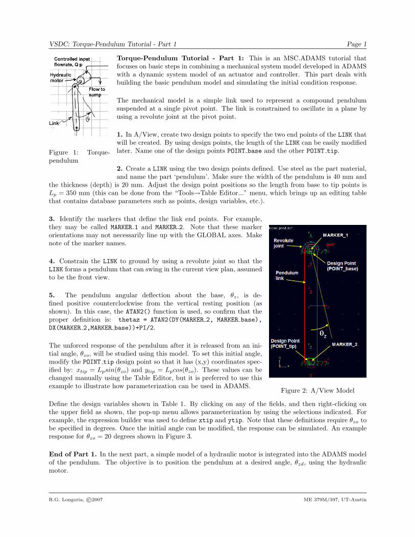
Figure 2: A/View Model
3. Identify the markers that define the link end points. For example,they may be called MARKER 1 and MARKER 2. Note that these markerorientations may not necessarily line up with the GLOBAL axes. Makenote of the marker names.
4. Constrain the LINK to ground by using a revolute joint so that theLINK forms a pendulum that can swing in the current view plan, assumedto be the front view.
5. The pendulum angular deflection about the base, θz, is de-fined positive counterclockwise from the vertical resting position (asshown). In this case, the ATAN2() function is used, so confirm that theproper definition is: thetaz = ATAN2(DY(MARKER 2, MARKER base),DX(MARKER 2,MARKER base))+PI/2.
The unforced response of the pendulum after it is released from an ini-tial angle, θzo, will be studied using this model. To set this initial angle,modify the POINT tip design point so that it has (x,y) coordinates spec-ified by: xtip = Lpsin(θzo) and ytip = Lpcos(θzo). These values can bechanged manually using the Table Editor, but it is preferred to use thisexample to illustrate how parameterization can be used in ADAMS.
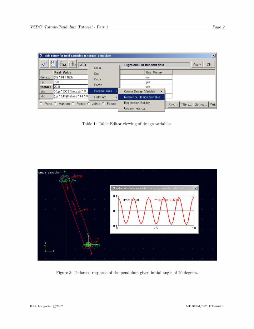
Define the design variables shown in Table 1. By clicking on any of the fields, and then right-clicking onthe upper field as shown, the pop-up menu allows parameterization by using the selections indicated. Forexample, the expression builder was used to define xtip and ytip. Note that these definitions require θzo tobe specified in degrees. Once the initial angle can be modified, the response can be simulated. An exampleresponse for θzo = 20 degrees shown in Figure 3.
End of Part 1. In the next part, a simple model of a hydraulic motor is integrated into the ADAMS modelof the pendulum. The objective is to position the pendulum at a desired angle, θzd, using the hydraulicmotor.
Torque-Pendulum Tutorial - Part 2: This part of the tutorial focuses on integrating a simple hydraulicmotor modle and position controller with the pendulum model built in ADAMS.
A hydraulic motor transforms power from hydraulic to mechanical form, ideally following the expressions,
Tm = DmPm
Qm = Dmωm
where m refers to ‘motor’ variables, Dm is the motor displacement (e.g., relates amount of fluid displacedper unit revolution). Real motors have friction and leakage, but these effects will be neglected here. Motorsmay also be influenced by compressibility of the fluid, and this can be accounted for by tracking volumetricfluctuations within the motor housing. This is a dynamic effect that will be included in this model becauseit allows us to show how a dynamic system model can be integrated within the ADAMS/View modelingenvironment.
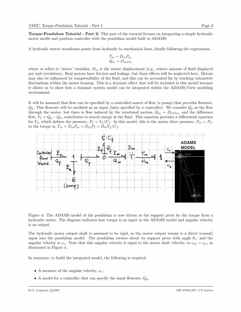
It will be assumed that flow can be specified by a controlled source of flow (a pump) that provides flowrate,Qp. This flowrate will be modeled as an input (later specified by a controller). We consider Qp as the flowthrough the motor, but there is flow induced by the rotational motion, Qm = Dmωm, and the differenceflow, V̇f = Qp −Qm contributes to stored energy in the fluid. This equation provides a differential equationfor Vf , which defines the pressure, Pf = Vf/Cf . In this model, this is the motor drive pressure, Pm = Pf ,so the torque is, Tm = DmPm = DmPf = DmVf/Cf .
Figure 4: The ADAMS model of the pendulum is now driven at the support pivot by the torque from ahydraulic motor. The diagram indicates how torque is an input to the ADAMS model and angular velocityis an output.
The hydraulic motor output shaft is assumed to be rigid, so the motor output torque is a direct (causal)input into the pendulum model. The pendulum rotates about its support pivot with angle θz, and theangular velocity is ωz. Note that this angular velocity is equal to the motor shaft velocity, so ωm = ωz, asillustrated in Figure 4.
In summary, to build the integrated model, the following is required:
• A measure of the angular velocity, ωz.
• A model for a controller that can specify the input flowrate, Qp.
• Representation of the differential equation, V̇f , which depends on Qp and on Qm = Dmωz.
• Representation of the torque model equation applied to the pendulum at the support pivot.
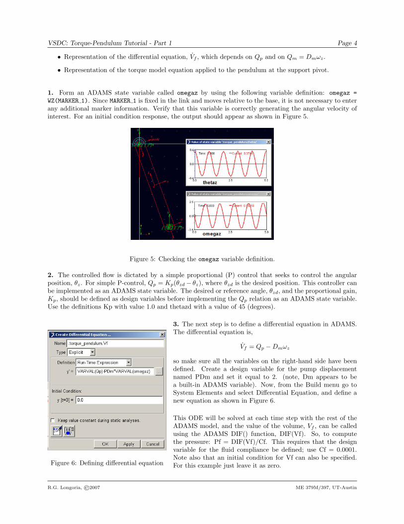
1. Form an ADAMS state variable called omegaz by using the following variable definition: omegaz =WZ(MARKER 1). Since MARKER 1 is fixed in the link and moves relative to the base, it is not necessary to enterany additional marker information. Verify that this variable is correctly generating the angular velocity ofinterest. For an initial condition response, the output should appear as shown in Figure 5.
Figure 5: Checking the omegaz variable definition.
2. The controlled flow is dictated by a simple proportional (P) control that seeks to control the angularposition, θz. For simple P-control, Qp = Kp(θzd − θz), where θzd is the desired position. This controller canbe implemented as an ADAMS state variable. The desired or reference angle, θzd, and the proportional gain,Kp, should be defined as design variables before implementing the Qp relation as an ADAMS state variable.Use the definitions Kp with value 1.0 and thetazd with a value of 45 (degrees).
Figure 6: Defining differential equation
3. The next step is to define a differential equation in ADAMS.The differential equation is,
V̇f = Qp −Dmωz
so make sure all the variables on the right-hand side have beendefined. Create a design variable for the pump displacementnamed PDm and set it equal to 2. (note, Dm appears to bea built-in ADAMS variable). Now, from the Build menu go toSystem Elements and select Differential Equation, and define anew equation as shown in Figure 6.
This ODE will be solved at each time step with the rest of theADAMS model, and the value of the volume, Vf , can be calledusing the ADAMS DIF() function, DIF(Vf). So, to computethe pressure: Pf = DIF(Vf)/Cf. This requires that the designvariable for the fluid compliance be defined; use Cf = 0.0001.Note also that an initial condition for Vf can also be specified.For this example just leave it as zero.
4. Now that volume is being determined by this dynamic equation, the motor torque can be found bydefining a state variable, Tm = DmPm = DmPf . In ADAMS syntax,
Tm = PDm*DIF(Vf)/Cf.
Once this torque is defined, a torque can be applied to the pendulum with a value determined by VAR-VAL(Tm). This last step should be completed.
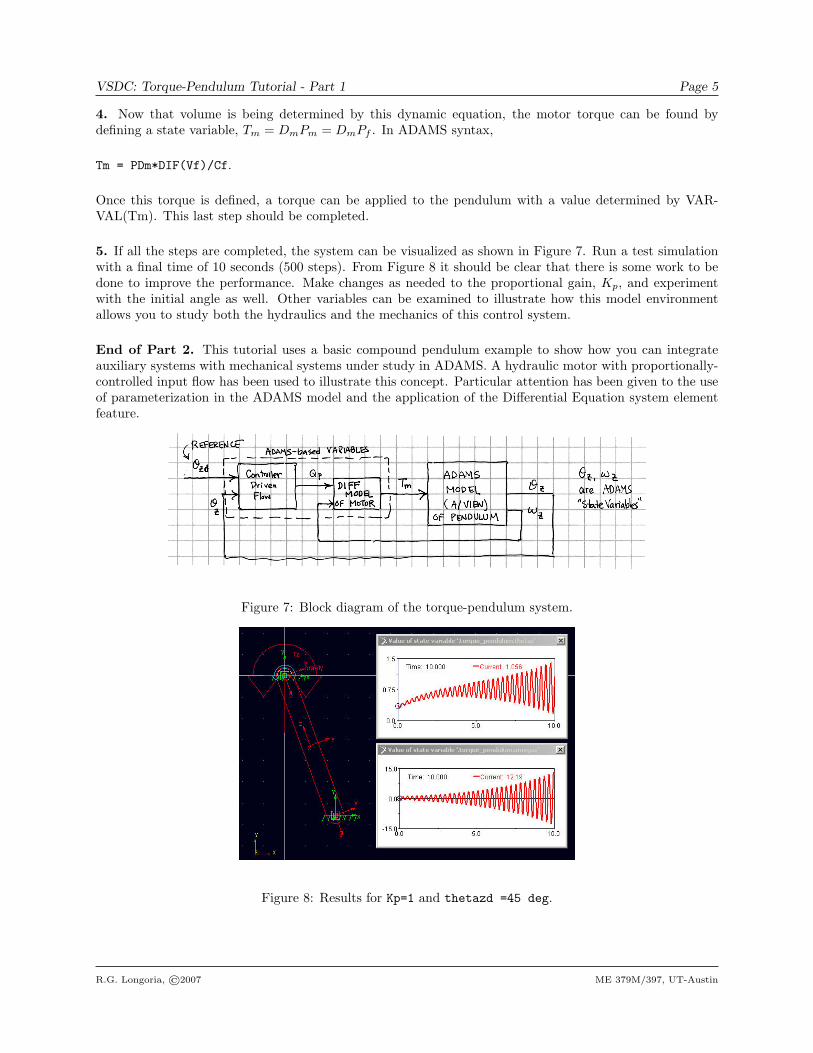
5. If all the steps are completed, the system can be visualized as shown in Figure 7. Run a test simulationwith a final time of 10 seconds (500 steps). From Figure 8 it should be clear that there is some work to bedone to improve the performance. Make changes as needed to the proportional gain, Kp, and experimentwith the initial angle as well. Other variables can be examined to illustrate how this model environmentallows you to study both the hydraulics and the mechanics of this control system.
End of Part 2. This tutorial uses a basic compound pendulum example to show how you can integrateauxiliary systems with mechanical systems under study in ADAMS. A hydraulic motor with proportionally-controlled input flow has been used to illustrate this concept. Particular attention has been given to the useof parameterization in the ADAMS model and the application of the Differential Equation system elementfeature.
Figure 7: Block diagram of the torque-pendulum system.