Page 1
University of Rhode Island University of Rhode Island
DigitalCommons@URI DigitalCommons@URI
Open Access Master's Theses
2016
Vulnerability Assessment of Steel Bridges Due to On-Deck Blasts Vulnerability Assessment of Steel Bridges Due to On-Deck Blasts
Justus Frenz University of Rhode Island, [email protected]
Follow this and additional works at: https://digitalcommons.uri.edu/theses
Recommended Citation Recommended Citation Frenz, Justus, "Vulnerability Assessment of Steel Bridges Due to On-Deck Blasts" (2016). Open Access Master's Theses. Paper 894. https://digitalcommons.uri.edu/theses/894
This Thesis is brought to you for free and open access by DigitalCommons@URI. It has been accepted for inclusion in Open Access Master's Theses by an authorized administrator of DigitalCommons@URI. For more information, please contact [email protected] .
Page 2
VULNERABILITY ASSESSMENT OF STEEL BRIDGES
DUE TO ON-DECK BLASTS
BY
JUSTUS FRENZ
A THESIS SUBMITTED IN PARTIAL FULFILLMENT OF THE
REQUIREMENTS FOR THE DEGREE OF
MASTER OF SCIENCE
IN
CIVIL AND ENVIRONMENTAL ENGINEERING
UNIVERSITY OF RHODE ISLAND
2016
Page 3
Use this page for the online version only. It will have the typed
names of the core committee, plus the Dean of the Graduate
School.
MASTER OF SCIENCE THESIS
OF
JUSTUS FRENZ
APPROVED:
Thesis Committee:
Major Professor Mayrai Gindy
George Tsiatas
Arun Shukla
Nasser H. Zawia
DEAN OF THE GRADUATE SCHOOL
UNIVERSITY OF RHODE ISLAND
2016
Page 4
ABSTRACT
Highway bridges are a critical element in the infrastructure for personal
transportation and movement of goods, yet they are constantly exposed to a number of
impacts and risks. One of these possible threats is an accidental or intentional
explosion on top of the bridge deck.
In this thesis, the effects of deterioration (in the form of section loss) of the
superstructure subjected to a blast load are analyzed for an example bridge. The
software ABAQUS and its CONWEP model were utilized to run a different scenarios
of section thicknesses reductions of the steel elements, varying thicknesses of the
concrete slab deck and the locations of the blast source.
The analysis output suggests that, for the blast load assumed in this thesis, only
small parts of the concrete deck structurally fail while the rest of the bridge remains
intact but permanently deformed in a way that a replacement of the bridge
superstructure after the explosion appears to be inevitable. Increasing section loss
obviously does have an impact on the deformations. However, the differences to the
initial bridge structure observed in the analysis are only minor as the zones of
structural failure and permanent deformations grow slightly but the overall stability
does not change fundamentally. So, even though the initial bridge performs better
when exposed to a blast event, initial and deteriorated bridges sustain permanent
deformations making bridge replacement necessary in both cases.
Page 5
iii
ACKNOWLEDGMENTS
I would first like to thank my thesis advisor Professor Mayrai Gindy of the Civil
and Environmental Engineering Department at the University of Rhode Island for
helping me to find a topic and her encouragement during the time of research and
writing of the thesis.
Besides my advisor, I would especially like to thank Professor George Tsiatas of
the Civil and Environmental Engineering Department at the University of Rhode
Island for answering questions, pointing to very interesting sources and providing
inspiration throughout the entire process.
My sincere thank also goes to Professor Arun Shukla of the Mechanical,
Industrial and Systems Engineering Department at the University of Rhode Island for
serving on my thesis committee as an outside committee member and Professor
Frederick J. Vetter of the Department of Electrical, Computer and Biomedical
Engineering at the University of Rhode Island for being the Chair of my Defense
Committee.
Finally, I would like to thank my family for providing me with unfailing support
and continuous encouragement throughout my years of study, especially the times
spent abroad.
Justus Frenz
Page 6
iv
TABLE OF CONTENTS
ABSTRACT .................................................................................................................. ii
ACKNOWLEDGMENTS .......................................................................................... iii
TABLE OF CONTENTS ............................................................................................ iv
LIST OF TABLES ....................................................................................................... vii
LIST OF FIGURES .................................................................................................... ix
CHAPTER 1: INTRODUCTION ................................................................................. 1
CHAPTER 2: REVIEW OF LITERATURE................................................................ 3
2.1 Blast Loading ..................................................................................................................... 3
2.1.1 Explosive Attack ......................................................................................................... 4
2.1.2 Event Location ........................................................................................................... 4
2.1.3 Explosive Materials .................................................................................................... 7
2.1.4 Blast event and Blast Wave Phenomena ................................................................... 9
2.1.5 Shock Loading .......................................................................................................... 13
2.1.6 Fragments ................................................................................................................ 15
2.1.7 Example Bridge ........................................................................................................ 16
2.2 Structural Response ........................................................................................................ 16
2.2.1 Structural System Behavior ..................................................................................... 17
2.2.2 Element Response ................................................................................................... 19
2.2.3 Material Properties and Strain Rate Effects ............................................................ 21
2.2.4 Bridge Design Specifications .................................................................................... 26
2.3 Simulation ....................................................................................................................... 27
2.3.1 Simulation Techniques for Impulse Loading ............................................................ 28
2.3.2 Software ................................................................................................................... 32
2.3.3 Verification/ Validation ............................................................................................ 32
CHAPTER 3: METHODOLOGY .............................................................................. 34
3.1 Research Approach ......................................................................................................... 34
3.1.1 Structural Steel Section Deterioration ..................................................................... 34
Page 7
v
3.1.2 Concrete Deck Deterioration ................................................................................... 36
3.2 AASHTO LRFD Guide Example Bridge ............................................................................. 38
3.2.1 General Information ................................................................................................ 39
3.2.2 Concrete Deck .......................................................................................................... 40
3.2.3 Steel Girder .............................................................................................................. 43
3.2.5 Assumptions ............................................................................................................ 52
3.3 Material Properties ......................................................................................................... 53
3.3.1 Concrete ................................................................................................................... 54
3.3.2 Reinforcement Steel ................................................................................................ 56
3.3.3 Structural Steel ........................................................................................................ 57
3.4 Bridge Loading and Boundary Conditions ...................................................................... 59
3.4.1 Extreme Event II ....................................................................................................... 59
3.4.2 Permanent Load....................................................................................................... 60
3.4.3 Transient Loads ........................................................................................................ 61
3.4.4 Blast Loading (BL) ..................................................................................................... 61
3.4.5 Boundary Conditions ............................................................................................... 62
3.5 Simulation Input ............................................................................................................. 63
3.5.1 Analysis Type ........................................................................................................... 63
3.5.2 Analysis Duration ..................................................................................................... 63
CHAPTER 4: FINDINGS .......................................................................................... 65
4.1 Initial Bridge (No Deterioration) ..................................................................................... 65
4.1.1 Concrete Deck .......................................................................................................... 66
4.1.2 Steel Girder Superstructure ..................................................................................... 74
4.1.3 Conclusion ................................................................................................................ 85
4.2 Deteriorated Bridges ...................................................................................................... 85
4.2.1 Deck Deterioration................................................................................................... 86
4.2.2 Steel Deterioration .................................................................................................. 93
4.3 Validation of the Model .................................................................................................. 99
4.3.1 System Deformation ................................................................................................ 99
4.3.2 Blast Pressure ........................................................................................................ 100
CHAPTER 5: CONCLUSION ................................................................................. 104
Page 8
vi
5.1 Effects of Section Reduction on the Structural Response ............................................ 104
5.2 Model accuracy ............................................................................................................. 105
5.2.1 Simulation .............................................................................................................. 105
5.2.2 Explosive Charge .................................................................................................... 105
5.2.3 Deterioration Assumptions .................................................................................... 106
5.3 Conclusion..................................................................................................................... 106
5.4 Further Research .......................................................................................................... 107
APPENDICES ........................................................................................................... 108
A.1 Static Deformation of the Example Bridge ................................................................... 108
A.2 Deck Reinforcement System Input ............................................................................... 112
BIBLIOGRAPHY ...................................................................................................... 114
Page 9
vii
LIST OF TABLES
TABLE PAGE
Table 1: Concrete and Reinforcement Steel DIF values .............................................. 23
Table 2: Structural Steel DIF values ............................................................................ 26
Table 3: Steel Deterioration Cases 0 to 4 ..................................................................... 35
Table 4: Steel Deterioration Cases 5, 10 and 20 .......................................................... 35
Table 5: Deck Deterioration Cases Overview .............................................................. 38
Table 6: Positive Moment Deck Reinforcement .......................................................... 41
Table 7: Negative Moment Deck Reinforcement ........................................................ 41
Table 8: Web, Stiffener and Cross Frame Thicknesses ............................................... 46
Table 9: Bottom Flange Thicknesses ........................................................................... 48
Table 10: Top Flange Thicknesses ............................................................................... 49
Table 11: Top Flange Widths ....................................................................................... 49
Table 12: Concrete General Material Properties .......................................................... 54
Table 13: Concrete Elastic Behavior............................................................................ 54
Table 14: Concrete Plasticity General.......................................................................... 54
Table 15: Concrete Plasticity Compressive Behavior .................................................. 55
Table 16: Concrete Plasticity Tensile Behavior ........................................................... 55
Table 17: Reinforcement Steel General Properties ...................................................... 56
Table 18: Reinforcement Steel Elastic Behavior ......................................................... 56
Table 19: Reinforcement Steel Property Modification ................................................ 57
Table 20: Reinforcement Steel Plasticity Input ........................................................... 57
Table 21: Structural Steel General Material Properties ............................................... 58
Page 10
viii
Table 22: Structural Steel Elastic Behavior ................................................................. 58
Table 23: Structural Steel Material Modification ........................................................ 58
Table 24: Structural Steel Plasticity Input ................................................................... 59
Table 25: Load Combination - Extreme Event II (AASHTO (2012)) ......................... 59
Table 26: Blast Loading Cases ..................................................................................... 62
Table 27: Deck Reinforcement, Negative Moment, No Deterioration ...................... 112
Table 28: Deck Reinforcement, Positive Moment, No Deterioration ........................ 112
Table 29: Deck Reinforcement, Negative Moment, Mild Deterioration ................... 112
Table 30: Deck Reinforcement, Positive Moment, Mild Deterioration ..................... 113
Table 31: Deck Reinforcement, Negative Moment, Severe Deterioration ................ 113
Table 32: Deck Reinforcement, Positive Moment, Severe Deterioration .................. 113
Page 11
ix
LIST OF FIGURES
FIGURE PAGE
Figure 1: Blast Location, Side View .............................................................................. 6
Figure 2: Blast Location, Plan View .............................................................................. 6
Figure 3: Pressure-time variation for Free-Air Burst (UFC 3-340-02, Department of
Defense (2014)) ............................................................................................................ 10
Figure 4: Free-air burst blast environment (Department of Defense (2014)) .............. 11
Figure 5: Structural Steel Stress-Strain Curve from UFC 3-340-02, Department of
Defense (2014) ............................................................................................................. 25
Figure 6: Possible Analysis Method Combinations (from NCHRP (2010)) ............... 29
Figure 7: Deck Deterioration, one Patch ...................................................................... 36
Figure 8: Deck Deterioration, two Patches .................................................................. 37
Figure 9: Deck Deterioration, four Patches.................................................................. 37
Figure 10: Deck Deterioration, six Patches.................................................................. 37
Figure 11: Static System, Example Bridge (FHWA, 2003) ......................................... 39
Figure 12: Superstructure Cross Section, Example Bridge (FHWA, 2003) ................ 39
Figure 13: Positive and Negative Deck Moment Regions ........................................... 41
Figure 14: Steel Girder Properties, Example Bridge (FHWA, 2003) .......................... 44
Figure 15: Steel Girder Properties, Model Input .......................................................... 45
Figure 16: Placement of Intermediate Stiffeners ......................................................... 46
Figure 17: Location of Intermediate Stiffeners ............................................................ 47
Figure 18: Model of Steel Elements............................................................................. 50
Page 12
x
Figure 19: Bearing Stiffener and Cross Frame Model ................................................. 51
Figure 20: Cross-Frame Model .................................................................................... 51
Figure 21: Bearing Stiffener at Abutment Support ...................................................... 51
Figure 22: Bearing Stiffener at Pier Support ............................................................... 51
Figure 23: Girder Naming for Analysis ....................................................................... 67
Figure 24: Vertical Deformation of Deck (Section 18.5m), Blast Case 1 ................... 67
Figure 25: Deformation Control Locations .................................................................. 68
Figure 26: Vertical Deformation of Span for two Control Points at time step 0.1 sec.,
Blast Case 1 .................................................................................................................. 69
Figure 27: Length of Deck Deformation ...................................................................... 69
Figure 28: Difference of Vertical Deck Deformation for Case: Steel 0 Deck 0 Blast 1
...................................................................................................................................... 70
Figure 29: Deck Failure Criteria Sketch ...................................................................... 70
Figure 30: Vertical Deformation of Deck Section 36.8 m at Time Step 0.1 sec. for
Blast Case 2 .................................................................................................................. 72
Figure 31: Difference of Vertical Deck Deformation for two Control Points at Time
Step 0.1 sec. ................................................................................................................. 73
Figure 32: Failure Criteria Case: Steel 0 Deck 0 Blast 2 ............................................. 73
Figure 33: Vertical Deformation of Girders at Time Step 0.005 sec. .......................... 75
Figure 34: Girder Location Naming [m] ...................................................................... 75
Figure 35: Vertical Deformation of Girders at Time Step 0.1 sec. .............................. 76
Figure 36: Vertical Deformation of Girders at Location 18.5 m ................................. 77
Figure 37: Absolute Rotation of Girder +3 at Abutment Support ............................... 78
Page 13
xi
Figure 38: Vertical Deformation of Girders at Time Step 0.15 sec. ............................ 78
Figure 39: Vertical Deformation of Girders at Time Step 0.2 sec. .............................. 79
Figure 40: Vertical Deformation of Girders at Time Step 0.05 sec. (Blast Case 2) .... 80
Figure 41: Vertical Deformation of Girders at Time Step 0.075 sec. (Blast Case 2) .. 81
Figure 42: Vertical Deformation of Girders at Time Step 0.1 sec. (Blast Case 2) ...... 81
Figure 43: Vertical Deformation of Girders at Time Step 0.125 sec. (Blast Case 2) .. 82
Figure 44: Vertical Deformation of Girders at Time Step 0.2 sec. (Blast Case 2) ...... 82
Figure 45: Vertical Deformation of Girder +3 at Location 36.8 m (Blast Case 2) ...... 83
Figure 46: Vertical Deformations of Girder +3 Case: Steel 0 Deck 0 Blast 1 - Long
Analysis (10 sec) .......................................................................................................... 84
Figure 47: Vertical Deformations of the Deck, Cases Steel 0 Deck 11, 12, 14 & 16 .. 86
Figure 48: Deformation Differences for Cases Steel 0 Deck 11, 12, 14 & 16............. 87
Figure 49: Vertical Deck Deformations for Cases Steel 0 Deck 21, 22, 24 & 26 ....... 88
Figure 50: Deformation Differences for Cases Steel 0 Deck 21, 22, 24 & 26............. 88
Figure 51: Vertical Deformations of Girder +3 at Location 18.5m for Cases Steel 0
Deck 11, 16, 21 & 26 ................................................................................................... 89
Figure 52: Vertical Deck Deformation at Section 36.8 m for Cases Steel 0 Deck 11, 12
& 14 (Blast Case 2) ...................................................................................................... 91
Figure 53: Deformation Differences for Cases Steel 0 Deck 11, 12, 14, 21, 22 & 24
(Blast Case 2) ............................................................................................................... 91
Figure 54: Vertical Deformation of Deck for Combined Deterioration (Blast Case 1) 92
Figure 55: Vertical Deformation of Girder +3 for Cases Steel 0, 1, 2, 3, 4, 5 & 10
Deck 0 .......................................................................................................................... 93
Page 14
xii
Figure 56: Maximum Vertical Deforamtion of Girder +3 for Cases Steel 0, 1, 2, 3, 4, 5
& 10 Deck 0 ................................................................................................................. 94
Figure 57: Vertical Deformation of Girder +3 at Time Step 0.092 sec for Cases Steel
0, 1, 2, 3, 4, 5 & 10 ....................................................................................................... 95
Figure 58: Vertical Deformation of Girder +3 at Location 18.5m for Cases Steel 0, 5,
10 & 20 Deck 0 ............................................................................................................ 96
Figure 59: Vertical Deformations of Girder +3 at Location 18.5m (Blast Case 2) ..... 97
Figure 60: Vertical Deformation of Girder +3 at Location 36.8m for Cases Steel 0, 1,
2, 3 & 4 Deck 0 (Blast Case 2)..................................................................................... 98
Figure 61: Vertical Deformation of Girder +3 at Location 36.8 m for Cases Steel 0, 5
& 20 Deck 0 (Blast Case 2).......................................................................................... 99
Figure 62: ABAQUS Result of Static Analysis ........................................................... 99
Figure 63: Blast Loading from CONWEP model for Point located under Blast Source
.................................................................................................................................... 101
Figure 64: CONWEP model loading at 0.0008 seconds ............................................ 101
Figure 65: CONWEP model loading at time steps 0.0013 sec. and 0.0035 sec. ....... 102
Page 15
1
CHAPTER 1: INTRODUCTION
Highway bridges are a vital part of the national infrastructure as they enable
transportation and traffic to cross rivers, valleys and other obstacles without diversion
or deceleration of the traffic flow. This outstanding function naturally creates a
bottleneck situation in the transportation network. Any restraints on this small network
element automatically result in major and far-reaching annoyance throughout larger
parts of the network. Bridge closures cause long diversions for road users and
overloading of other roadways. Therefore, the serviceability of bridges is of great
economic importance and high public interest.
To provide the desired level of functionality, bridges have to be designed and
maintained to resist a variety of impacts from traffic and wind loading, but also
weathering and aging. To continuously guarantee a certain level of safety, they have to
be surveyed and assessed on a regular basis. Depending on a variety of factors,
officials schedule recurring condition surveys of their assets so that the structural
health of the structure is known at all times and reevaluation of load allowance,
maintenance, or replacement can be carried out as necessary.
One imaginable impact to every highway bridge is an on-deck blast event.
Explosions on roadway bridges could be caused inadvertently in accidents or
intentionally as part of an attack trying to disrupt the transportation network. Bridges
are critical infrastructure assets and choke points of traffic flow, yet very accessible
and difficult to protect which could make them a potential target.
Page 16
2
Currently, the on-deck blast scenario is not routinely considered during the design
process of regular highway bridges. Manuals and recommendations exist for blast
resistant design of bridge substructures (namely pier columns) and, of course, for
protective structures, but not for bridge decks and superstructures. The sixth edition of
the AASHTO ‘LRFD Bridge - Design Specifications’ (2012) only provides a set of
references for blast loading and analysis but no specific requirements. Likewise, no
information is available to examine, how bridge deterioration affects the bridge
resistance capacity to blast loading.
In this thesis, the effect of bridge deterioration (namely cross section reduction) to
blast loading resistance is examined.
Upon review of current literature on blast loading, structural response and blast
simulation in Chapter 2, the methodology of the analysis is discussed in Chapter 3.
Here, the research approach, the software inputs such as material characterization, the
example bridge, and analysis options are presented.
Chapter 4 comprehends the findings of the analysis outputs in three categories. In
a first step, the original bridge is exposed to blast loadings at different blast locations
to identify a characteristic bridge behavior after the detonation. In a second step,
bridges with deteriorated elements are exposed to the same blast loadings. Here, the
effects of the deteriorations by location can be assessed. Lastly, bridges with
deterioration combinations in more than one structural element are studied.
In the final chapter (Chapter 5), conclusions from the findings of Chapter 4 are
discussed.
Page 17
3
CHAPTER 2: REVIEW OF LITERATURE
This chapter presents a comprehensive review of both current and established
literature relevant for the topic of on-deck blast loading. The literature review is
composed of a sequential presentation:
Section 2.1 examines the explosion and blast loading, characterizing the
explosive attack, comparing different explosive materials, discussing the propagation
of the shock wave, and shock phenomena on structures.
Section 2.2 subsequently describes the structural response to such shock loadings.
The sub-categories include structural system behavior, element response, material
properties with strain-rate effects, and failure criteria.
In Section 2.3, the simulation of the problem is presented. Here the simulation
techniques, utilized software and the validation of the analysis output are discussed.
2.1 Blast Loading
In this section, a blast scenario is characterized and parameters necessary to
simulate the event are presented. In a previous step, possible blast scenarios have to be
identified in a risk assessment for every individual bridge. The topic ‘blast risk
assessment’ will not be presented in this thesis (a step-by-step risk assessment process
can, for example, be found in ‘Guide to Highway Vulnerability Assessment for Critical
Asset Identification and Protection’, SAIC (2002)).
Page 18
4
2.1.1 Explosive Attack
The output of the Risk Assessment is ultimately the identification of one or more
possible attack scenarios that the bridge might be exposed to. It has to be checked
whether those events compromise bridge’s structural integrity and/or serviceability in
an extent deemed unacceptable by decision makers. In the following sections, the
qualitative determination of possible threats is converted into quantifiable impacts to
the structural model.
The most relevant characteristics of the explosion include:
- the weight of the explosive charge
- the distance between the explosive and the structure
- the angle of impact
- the impact of fragments
2.1.2 Event Location
A variety of several blast locations might be critical for the bridge, depending on
the bridge type.
For many bridge types, explosions under the span are highly concerning. Most of
all, the blast impact from underneath possibly leads to a load reversal in many
structural members which can lead to element failure as well as components being
lifted out of their usual bearing positions. Also, fatally compromising the substructure
and foundation inevitably results in a collapse of the superstructure. Furthermore,
underside explosions are somewhat confined so that reflections of the blast wave can
Page 19
5
significantly magnify the impact, for example in small spaces near abutments or in
between girders (Williamson and Winget 2005).
For most cable bridges, locations around or especially inside of the tower are very
critical as a tower failure would lead to a collapse of the entire bridge. Unless
explosions are especially set up to cut a number of cables, on-deck blast is not likely to
cut cables accidentally due to their extremely small area and round shape as well as
their flexibility (Williamson and Winget 2005).
For box girders, internal explosions are the most critical as the confinement
pressure could lead to failure (Williamson and Winget 2005).
Nevertheless, one scenario applicable to all bridge types is the on-deck blast event
examined in this report. Many of the aforementioned attacks can be avoided by simple
limitation of accessibility. For example, the access to bridge towers and the inside of
the box girder can be controlled and monitored. Explosions from below the bridge
may also be controlled by avoiding parking spaces under the bridges, restricting access
paths or for the case of a highway bridge, the lower road can be channeled away from
the bridge supports and substructure by permanent barriers making the critical points
difficult to access. The very controlling parameter ‘standoff distance’ between the
charge and the object can thereby be increased significantly. In contrast, on-deck
access to bridges cannot be restricted without major interference of the bridges
original purpose of serving as a roadway (e.g. weight restrictions for cars and trucks).
Risk mitigation methods can also include car and truck searches before they are
allowed onto the bridge. This extreme method however heavily impacts the flow of
the traffic.
Page 20
6
As this thesis focusses on on-deck explosions, the standoff distance is very small
and only consists of the distance between the center of the charge and the bridge deck
surface. For the following report, two location scenarios will be considered:
Location 1 is a charge located at midspan with a height of 6 ft. 7 in. (2.0 m)
for a one-span collapse (Blast Case 1).
Location 2 is a charge placed directly above the center pier at 6 ft. 7 in.
(2.0 m) possibly leading to substructure failure and/or a two
span collapse (Blast Case 2).
Side View:
Abutment Support Pier Support Abutment Support
Figure 1: Blast Location, Side View
Plan View:
Figure 2: Blast Location, Plan View
The Example Bridge will be presented thoroughly Chapter 3 (Section 3.2).
Location 2 Location 1
Location 2 Location 1
Travel Lane – 12’
Travel Lane – 12’
Shoulder - 10’
Shoulder - 10’
Page 21
7
2.1.3 Explosive Materials
Explosive materials can be classified by their physical state (solid, liquid or
gasiform) with different blast pressure environments being produced by each material
during the explosion. Blast effects generated by high-explosive, solid materials are
best known. Their blast pressure distributions, impulse loading, characteristic loading
durations and other effects of the explosion are well established (Department of
Defense, 2014). In the following, these characteristics are presented for the solid
explosive material TNT (Trinitrotoluene).
2.1.3.1 TNT Equivalency
Across the reviewed literature, TNT was the one material chosen for the analysis.
Even though other materials might actually explode in the scenario, efforts were made
to convert the amount of this other material into the amount of TNT that would release
the same heat and therefore has a similar effect on the structure and the surroundings.
The explosive charges are characterized by the TNT-equivalent weight ([lb] or [kg])
of the explosive. However, since condensed high explosive produce similar
characteristic blast waves, with an adjustment of the weight, the effects of different
explosives can be modeled sufficiently with the TNT approach. The TNT equivalent
charge weight is determined by (Conrath et al. (1999)):
Page 22
8
𝑊 = (𝛥𝐻𝐸𝑋𝑃
𝛥𝐻𝑇𝑁𝑇) ∗ 𝑊𝐸𝑋𝑃
ΔHEXP Heat of detonation of explosive in question
ΔHTNT Heat of detonation of TNT
WEXP Weight of explosive in question
In the following, all charge weights will always be referred to as TNT-equivalent
weights.
2.1.3.2 Charge Weights
All explosions analyzed in this thesis propagate through air, the detonation
location has been identified at a standoff distance of 6 ft. 7 in. above the roadway (the
change in location on the bridge does only effect the blast in an uncoupled analysis
(see Section 2.3.1.2)), the type of explosive is always TNT (other explosive materials
are expressed as a TNT equivalent weight charge) and the casement will be neglected
in this study.
Thus, the next critical detonation parameter is the amount of explosive as
described in the charge weight. Conrath et al. (1999) describe the weight limits that
can be assumed by designers for different kind of aggressors. For instance, a handheld
explosive, that is carried by the attacker and placed near the structure, can be assumed
as a 50 lbm (23 kg) charge. For the vehicle mode of attack in which a vehicle such as a
car or truck is driven onto or abandoned near the critical structure, the weight is only
limited by the carrying capacity of the vehicle. The Blue Ribbon Panel on Bridge and
Page 23
9
Tunnel Security’s recommendations (2003) include a table of possible magnitudes of
threats. For conventional explosives, the ‘Highest Probability’ car bomb size is 500
lbs. The ‘Largest Possible’ threat, which could pass onto the bridge unnoticed, is
quantified as a truck bomb with a weight of 20,000 lbs. In this report, the most
probable value is assumed:
Example Charge Weight: 500 lbs. (Blast Cases 1 & 2)
Instead of using a safety factor associated with impacts and resistance during the
check, the Department of Defense (2014) recommends to increase the TNT equivalent
charge weight by 20 percent into an effective charge weight. This is to compensate for
any kinds of unknowns.
As the charge weight is a very critical design parameter in the determination of
the blast impact on the structure, this recommendation will be applied. The effective
charge weight is (Blast Cases 1 & 2):
Charge Weight Effective Design Charge Weight
Example Charge: 500 lbs. . 600 lbs. (272.6 kg)
2.1.4 Blast event and Blast Wave Phenomena
Detonations are described as sudden, violent release of energy in a comparatively
small area. The explosive material is being converted into very high pressure gas at
very high temperatures leading to a pressure front that propagates outwards spherically
into the surrounding atmosphere until it is disturbed by any kind of confinement or
barrier.
Page 24
10
The pressure front released during the explosion, or blast wave, travels away from
the burst point and is characterized by (Department of Defense, 2014):
- a time tA as the duration of travel of the blast wave front through the medium
until it impacts the surface,
- a positive peak pressure (much) greater than the ambient pressure PS0,
- a pressure decay back to the ambient pressure and
- a negative pressure phase with a pressure below the ambient pressure which is
usually a lot longer than the positive phase but less important for the design.
The incident impulse for both the positive and negative phase can be determined
by integrating the area under the curve of the respective phase.
Figure 3: Pressure-time variation for Free-Air Burst (UFC 3-340-02, Department of
Defense (2014))
Pre
ss
ure
Time
Pressure-time variation for Free-air Burst
Ambient P0
tA + t 0 tA + t0+ t0-
Positive Phase,
Duration: t 0
Negative Phase,
Duration: t 0-
Peak Incident Pressure PS0
Negative Pressure PS0
-
Blast t=0
tA
Page 25
11
Depending upon boundary conditions such as detonation location and
confinement, the parameters vary greatly. The scenario of on-deck blast can be
characterized as an unconfined explosion because the pressure wave can diffuse freely
in three directions (radially and upwards), so that only the original blast wave
travelling from the burst point impacts the deck. No reflected wave or pressure build-
ups are expected to occur at the bridge deck surface.
UFC 3-340-02, Department of Defense (2014) defines ‘Free Air Bursts’ as
detonations that occur “adjacent to and above a protective structure such that no
amplification of the initial shock wave occurs between the source and the protective
structure”.
Figure 4: Free-air burst blast environment (Department of Defense (2014))
In this blast environment, the point of the surface located normal under the burst
point has to sustain the greatest normal incident pressure and impulse. For all other
points on the bridge deck, the peak pressure and impulse have to be modified with
Page 26
12
regards to the increasing distance from the burst point and the angle of incidence. The
modification reduces the size of the impact.
For some design applications, the negative shock phase is also implemented in the
loading-time function of the structural response to the blast load. In steel structures
such as frames, the overall motion is affected by this phase. In more rigid structures,
(namely) reinforced concrete, the effects of this phase are not of high significance
(UFC 3-340-02, Department of Defense (2014)). In this analysis, the CONWEP model
includes the negative phase automatically. However, the phase is also relevant for the
behavior as the structural steel components of the composite bridge have a significant
influence on the overall load bearing characteristic of the structure.
Other types of Unconfined Explosions include ‘air bursts’ and ‘surface bursts’
(UFC 3-340-02, Department of Defense (2014)). Both of these types include reflected
blast waves from either the ground or other object faces in proximity of the blast event
in the analysis and focus on horizontal surfaces. They are therefore not applicable for
this analysis.
For large distances between the charge and the surface of the structure, a few
simplifying assumptions can be made. For example, the wave front can be assumed as
planar so that the entire surface is impinged by the same characteristic blast wave
pressure-time impact allowing for a faster analysis. (UFC 3-340-02, Department of
Defense (2014))
For close-in explosions such as in this analysis, this assumption of a constant
pressure-time impact along the entire surface is not acceptable and a significant
overestimation of the impact would yield unrealistic, very conservative results. Also,
Page 27
13
the difference of arrival time of the shock front cannot be disregarded. Therefore,
close-in explosion accuracy has to be employed (UFC 3-340-02, Department of
Defense (2014)). Again, this is automatically accomplished by the CONWEP model
(Section 2.3.2) utilized in this analysis.
2.1.5 Shock Loading
Blast loading differs significantly from other impacts in civil engineering design.
Among the differences are the duration of the loading process (sudden/ impulsive
instead of static) and the duration of the load being present on the structure. The blast
duration is measured in milliseconds, which, as a scale, is magnitudes shorter than the
unit of seconds during wind impact analysis or very long time spans for quasi-static
loads.
2.1.5.1 Loading Types
Gündel et al. (2010) describe three different characteristic types of loading. Dead
load such as gravity, but also certain live loads can be treated as ‘static’ or ‘quasi-
static’. These loads are not subject to fast changes and remain on the structure for a
relatively long time, so only the absolute value of the load is required during the
design process. The duration of these loads is greater than three times the natural
period of the structural element.
Quasi-static loading: td/T > 3
Page 28
14
In contrary, wind or earthquakes cause dynamic loading to the structure. For the
design process, the load-time distribution is relevant and necessary, as this impact has
a high time dependency and the response is partly governed by the dynamic
characteristics of the element.
Dynamic loading: 0.3 < td/T < 3
In this analysis, short-duration dynamic loads are being studied. The structure is
being exposed to the nonoscillatory pulse loads of an explosion that only last
milliseconds. In this domain of load durations much smaller than the elements natural
period, inertia has to be taken into account. Thus, other principles and checks have to
be applied to control the structural response to this type of impact.
Impulse loading: 0.3 > td/T
2.1.5.2 Detonation Loading
Conrath et al. (1999) identify three principal products of a detonation, all of
which are dependent on standoff distance, media through which the blast propagates,
casement, charge weight, and type of explosive.
- Total Impulse Delivered
- Peak Pressure Delivered
- Delivered Velocity, Distribution and Mass of Fragments
As stated previously, a time-dependent pressure variation must be established for
the design process. For structural loading, the dynamic pressure is the controlling
Page 29
15
input. It can be determined from charts (e.g. Figure 2-3, UFC 3-340-02, Department of
Defense (2014)) as relationship between the incident shock pressure (Section 2.1.4)
and the dynamic pressure is established. In this analysis, the CONWEP model
(Section 2.3.2) will be used to determine blast pressures on the structure instead of
hand calculations. The figures from UFC 3-340-02, Department of Defense (2014)
will be utilized to for the validation of the CONWEP model input to check the impact
to the structure.
2.1.6 Fragments
Fragments are another important product of explosions. They can be divided into
two categories (UFC 3-340-02, Department of Defense (2014)).
- Primary Fragments are produced by the casing or objects in intimate contact
with the explosive. These fragments are very small but travel at very high
velocities.
- Secondary Fragments (or “debris”) produced by the blast wave interaction
with objects and structures in close proximity of the explosive source.
For structural analysis, Conrath et al. (1999) suggest to either neglect fragments
as the blast wave has the governing impacts throughout the design or implement an
assumption for a pre-damaged concrete surface (exposed concrete face is assumed
with spalls or craters) when the blast wave arrives at the structural surface.
Page 30
16
Both types of fragments are not considered in this analysis as they only impact
the upper surface of the concrete road deck and are assumed to have only a subsidiary
impact.
2.1.7 Example Bridge
For this analysis of an explosion on top a steel girder bridge and the effects of
structural deterioration on the bridge’s resistance, a typical bridge has to be identified.
In the following, the LRFD design example bridge will be used as it is specified in
FHWA NHI-04-041 (2003). This assumption eliminates the need for an assessment of
typical bridges and the exemplary design of a bridge for this report. The bridge
implemented in the model is described in Chapter 3.
The blast cases have been identified through this literature review and not through
an exemplary risk assessment as no parameters are available and too much input data
would have to be assumed. The blast loading has been characterized in Sections 2.1.2
and 2.1.3.2.
2.2 Structural Response
Blast impacts present unique challenges for structures. Very short, highly
impulsive impacts do not occur during any of the other loading types the structure was
initially designed for. However, the structural response is very dependent on the rate
of loading.
Page 31
17
2.2.1 Structural System Behavior
Explosions present an extreme loading event with a great amount of energy to be
dissipated by the structure in order to prevent failure or total collapse. Therefore, an
elastic and inelastic response with large deformations are to be expected until the
kinetic energy of the impact is dissipated with strain energy of deflection and/or partial
or total collapse occurs due to fragmentation of concrete. Design provisions such as
span length, element height and detailing of reinforcement determine the deflection
capabilities of a reinforced concrete structural element. UFC 3-340-02 (Department of
Defense (2014)) describes the following structural behavior:
At a deflection associated with 2° (degree) support rotation, tension reinforcement
has yielded and compressed concrete may begin to crush. Reinforced concrete
elements without shear reinforcement will fail at this level of deflection.
Shear-reinforced structural elements have the capacity to transfer the compressive
force to the compression rebar thus preventing failure until such members fail at about
6° (degree) support rotation.
If truss action can develop, the failure can be prevented until a support rotation of
approximately 12° (degrees) is reached. This is only possible if lateral restraint is
available to develop sufficient in-plane tensile forces.
Additionally, the shear capacity has to be adequate to prevent abrupt failure at
lower loading levels due to shear so that the aforementioned flexural failure resistance
can be utilized. The structural nonlinear response is also heavily dependent on the
redundancy of the system, but no universal solution can be identified. Indeterminate
structures have advantages with redistributing loads with their inherent capability to
Page 32
18
create alternate load paths. However, they usually also restrain deformation and
therefore might have a smaller capacity to dissipate energy with plastic deformations.
Therefore, structures with greater structural ductility, larger spans and mass have an
advantage. According to UFC 3-340-02, Department of Defense (2014), two modes of
structural behavior can be identified: Ductile (associated with large deflections
without complete collapse) and Brittle (partial failure or total collapse or the element).
In structural behavior to blast, ductile elements have a substantial advantage over
brittle. Brittle materials fail abruptly while ductile members are capable of developing
plastic hinges in regions of maximum moment. In reinforced concrete for example, a
plastic hinge can develop, when the tension reinforcement yields and then compressed
concrete is crushed and/ or compression reinforcement buckles UFC 3-340-02,
Department of Defense (2014).
2.2.1.1 Failure Criteria
A variety of physical parameters are available to monitor the structural health of a
structure during the process of blast loading. Commonly, either rotations or deflections
are utilized as system performance indicators as they are easily obtainable from a
structural simulation.
In this analysis, 2° support rotation as identified by UFC 3-340-02, Department of
Defense (2014) is used as the failure criteria during the assessment for both concrete
slabs and steel girders.
In addition, compression failure criteria of steel columns as suggested by Conrath
et al. (1999) will be used during the analysis evaluation. ‘Light’, ‘Moderate’ and
Page 33
19
‘Severe’ damage of the steel column are characterized by height shortening under
compression of 2 %, 4% and 8 % respectively.
2.2.2 Element Response
Individual structural elements may have different response times than the overall
system. While long-span elements are able to deform, short or stiff elements might fail
abruptly. Flexural modes of element response are more favorable, the greater flexural
ductility can dissipate more energy than shear deformations.
During the analysis of an element, two steps are of importance. First, the effects
of the detonation on the particular member have to be understood and checked. And
regardless of the response of the single member is (deflection, failure, etc.), the impact
on adjoining elements and the effect on the overall structural integrity have to be
assessed. The failure of a single element might lead to failure of one or more adjoining
elements that did not structurally fail during the blast loading.
In this analysis, a full bridge model so that interactions between the individual
elements are included automatically.
2.2.2.1 Global Response
Detonations at great standoff distances are expected to cause global element
responses. This means that the design case can be associated with a set of assumptions
for the structural design process. Elements subjected to such impacts are expected to
resist with flexural response mechanism of the full length of the elements. Hinges
Page 34
20
(either plastic hinges or support bearings) have to be available to allow for the
adequate rotations.
A flexural response mechanism is very desirable as it is ductile and has the
capability of dissipating great amounts of energy. Bending is also associated with
lower strain rates thus demanding less ultimate resistance of elements. Damage is
mainly induced by wave propagation resulting in concrete spalling on the far side and
concrete crushing on the impacted face of the element.
However, great attention has to be paid to connection detailing as hinge support
or beam slips form support can occur at lower loading level than shear or flexural
failure. (Conrath et al. (1999))
2.2.2.2 Local Response
Close-in detonations are associated with a different element response type.
Structural members subjected to more localized, non-uniform impacts have to resist
localized direct (dynamic) shear resulting in punching shear response types. These
impacts are typically linked with higher strain rates.
Other than from small standoff distances, local responses are also observed at
points of geometric or load discontinuity such as cross-section variation or discrete
ends of protective shielding of the element.
Elements subjected to close-in impacts have to be designed for large deflection
and need specialized, advanced reinforcement detailing to ensure a ductile response. If
this is not the case, the element is likely to fail due to the high-pressure concentrations
in a brittle failure mode.
Page 35
21
Concrete tends to react with spalling, cratering, scabbing as well as direct shear.
Also, the hinges and supports have to capable to resist the sudden shear stress induced
by the detonation. (Conrath et al. (1999))
2.2.3 Material Properties and Strain Rate Effects
At high strain rates, material properties change considerably from the
characteristic values under static loading. However, techniques are available consider
those complex strain rate effects and calculate the strength increase at a given strain
rate. Neglecting these phenomena would be a source of inaccuracy because material
ductility and strength are very important parameters in the bridge response and
behavior to blast effects. Also, the strength increase contributes to a more economic
design result.
UFC 3-340-02, Department of Defense (2014), propagates the introduction of
two different factors for both concrete and steel.
The Dynamic Increase Factor (DIF) is defined as the ratio of Dynamic Material
Strength to Static Material Strength. As strain rates vary significantly between static
loading and those present in blast events, this factor adjusts material properties to the
impulse loading case.
Strength Increase Factors (SIF) account for realistic material properties under
dynamic loads. Additionally, Age Increase Factors can be used to account for concrete
gaining strength beyond the nominal capacity at 28 days.
Page 36
22
2.2.3.1 Reinforced Concrete
Even though concrete has to be classified as a brittle material, reinforced concrete
demonstrates ductile behavior so that it can be considered as a ductile construction
method. This performance is dependent on reinforcement bars being tied and anchored
sufficiently.
The concrete strength has a great influence on the behavior of element, namely
the shear capacity. In stronger concrete materials, shear reinforcement may be
reduced. Also, at larger support rotations of elements, stronger concrete exhibits less
cracking and crushing. Especially for elements with large support rotations of more
than 2 degrees, the concrete strength only has a minor influence on ultimate strength
of elements.
UFC 3-340-02, Department of Defense (2014), provides recommendations for
minimum material qualities to be used for structural building materials in blast design.
For concrete, a minimal compressive strength of min f’c = 4 ksi is recommended.
Under no circumstances, the concrete material strength should be less than f’c = 3 ksi.
Research by Yi et al. (2013) shows, that higher concrete strength exhibits fewer
numbers of failure mechanisms, however the likelihood of brittle failure during
simulations at higher loads increases. Brittle failure should be avoided on a general
principle. During the analysis, a compromise between high material strength and
danger of brittle failure has to be identified.
For in-situ applications, performance testing of the existing concrete might be
desirable as the in-place strength could be greater than the nominal strength. This
increase in resistance is very beneficial for the analysis of the structural capacity.
Page 37
23
A estimate of DIFs for design purposes are given in UFC 3-340-02, Department
of Defense (2014). These values are more conservative for shear and bond than for
bending and compression. This can be justified by the brittle failure mechanism
associated with shear and bond failure which is less desirable and more dangerous thus
a reduced resistance capacity can be accepted. For a preliminary design, DIF values
can be obtained from the Table 4-1(UFC 3-340-02, Department of Defense (2014)). In
the table below, the values for ‘Bending’ in the ‘Close-In’ design range are presented:
Table 1: Concrete and Reinforcement Steel DIF values
Type of Stress
Close-In Design Range
Reinforcing Bars Concrete
fdy/fy fdu/fu f’dc/f’c
Bending 1.23 1.05 1.25
For more accurate values, the concrete DIF can be adjusted with respect to the
actual strain rate. A higher strain rate results in a higher ultimate compressive strength
of the concrete (for example, Figure 4-9 from UFC 3-340-02, Department of Defense
(2014), not applied in this analysis).
No Strength Increase Factor (SIF) is applied: SIF = 1.0.
2.2.3.2 Reinforcement Steel
Reinforcement should be of Grade 60 with bars smaller than No. 11 bars for
ductility purposes. Larger bars are undesirable because of the spacing and anchorage
requirements. On a general basis, ductility and thereby resistance is reduced at bends
and splices. Anchorages should not be avoided near the points of maximum stress.
Page 38
24
For accurate calculations of ultimate resistance of an element, stress-strain
relationships for the reinforcement should be known. Characteristic values for Grade
60 reinforcement (for ASTM A 615) are:
Fy = 60 ksi and Fu = 90 ksi
The SIF for the yield stress can be assumed as SIF = 1.1 so that the recommended
design values are
Fy = 66 ksi and Fu = 90 ksi
The DIF values for the design process can be found in the table in Section 2.2.3.1.
Again, for a more accurate and detailed analysis, strain rate dependent DIF values can
be obtained (for example Figure 4-10 from UFC 3-340-02, Department of Defense
(2014), not used in this analysis).
2.2.3.3 Structural Steel
Just as reinforcement bars, structural steel is strong and ductile. It is characterized
by yield stress, ultimate tensile strength, elongation at rupture and modulus of
elasticity. All of these properties vary with the duration of the impact compared to the
natural frequency of the element thus being subject to strain rate effects.
Like in reinforcement, a yield strength increase of 10 % can be assumed for steel
other than high strength steel, for which this assumption might be unconservative
(UFC 3-340-02, Department of Defense (2014)).
SIF = 1.1 for Fy = 50 ksi or less
SIF = 1.0 otherwise
Page 39
25
The mechanical properties are illustrated in the plot shown below. The yield point
increases significantly while the ultimate tensile strength only increases slightly. This
is captured in two different DIFs for yield strength and ultimate tensile strength
respectively. The modulus of elasticity and the elongation at rupture do not change
significantly. The figure below presents the static and the dynamic stress-strain
relationship.
Figure 5: Structural Steel Stress-Strain Curve from UFC 3-340-02, Department of
Defense (2014)
The DIFs for yield strength and ultimate tensile strength for general design are
tabulated for some materials. Table 5-2 from UFC 3-340-02, Department of Defense
(2014) only lists Steel Materials A36, A588 and A514 while the design material
values for the example bridge in this analysis suggest that a A572 Grade 50 has been
used (fy = 50 ksi and fu = 65 ksi). The following dynamic increase factors (DIF) have
been assumed for this analysis:
Page 40
26
Table 2: Structural Steel DIF values
Material
Bending
Ultimate Stress DIF
High Pressure
fdy / fy fdu/fu
A572 Grade 50 1.24 1.1
More accurate, strain-rate dependent DIFs for the yield strength of different steel
materials can be taken from graph such as Figure 5-2 (UFC 3-340-02, Department of
Defense (2014), not used for this analysis).
Generally, steel structures and members are not designed for excessive
deflections so that strain-hardening of steel should not be occurring in the element.
Just as for concrete, a stronger material does not automatically result in better
blast resistance. Son et al. (2012) have identified that medium-strength steel actually
exhibits better behavior against blast loading than high-strength.
2.2.4 Bridge Design Specifications
The 6th
Edition of the AASHTO LRFD Bridge Design Specification (2012)
features a section on the loading scenario ‘Blast’. However, the manual only provides
a qualitative list of relevant aspects during the design without quantitative provisions,
suggestions or regulations. It states that results obtained from an equivalent static
analysis should not be used for the design. A list of references is featured in the
manual, for example:
- AASHTO’s Bridge Security Guidelines (2011)
Page 41
27
- Baker et. al. (1983) ‘Explosion Hazards and Evaluation’
- Biggs’ (1964) ‘Introduction to Structural Dynamics’. This work presents
dynamic analysis approaches for a large number of systems ranging from one-
degree to multidegree systems and design applications. The chapter on ‘Blast-
resistant Design’ focusses on Nuclear Explosions and Protective Structures.
- Bounds (1998) ‘Concrete and Blast Effects’
- Bulson (1997) ‘Explosive Loading of Engineering Structures’
- Conrath, et al. (1999) ‘Structural Design for Physical Security: State of
Practice’
- Department of the Army, 1986 and 1990. The manual unfortunately does not
specify these referenced documents any further. They could refer to
publications ’TM 5-855-1 : Fundamentals of Protective Design for
Conventional Weapons’ (1986) and ‘TM 5-1300 : Structures to Resist the
Effects of Accidental Explosions’ (1990, which has since been superseded by
UFC 3-340-02 (Department of Defense, 2014)).
Another available design manual is ‘Blast-Resistant Highway Bridges: Design
and Detailing Guidelines’ (NCHRP Report 645, 2010). It focusses solely on the
substructure of the bridge, namely columns, but not the superstructure.
2.3 Simulation
To analyze blast events on structures, equations and/or numerical simulations are
commonly utilized since large scale testing is very expensive and often times not
Page 42
28
desirable or available. In the process, two tasks have to be accomplished. First, the
blast event has to be simulated resulting in an energy and pressure wave output. This
output then has to be applied to the structure as a load. The techniques to accomplish
the simulation are outlined in the first part of this section.
Subsequently, this section introduces the software used for the numerical analysis
and the approach for the validation of the model.
2.3.1 Simulation Techniques for Impulse Loading
For the simulation of blast-structure-interaction, many basic principal approaches
are available. Each approach has an inherent level of the input data requirement,
complexity of simulation and quality of output results. According to NCHRP Report
645 (2010), the approaches can be classified by three basic characteristics:
- Coupled/ Uncoupled Analysis
- Static or Dynamic Analysis
- Number of Degrees of Freedom (DOF)
The chart below compares different types of analysis type combinations. While a
coupled, dynamic analysis with multiple degrees of freedom promises the most
accurate simulation results, it is also the most complex, extensive and costly approach.
This results in long computation durations and comprehensive input requirements. An
uncoupled, static analysis with only one degree of freedom, in contrast, is simple and
quicker, however the results must be expected to be less accurate.
Page 43
29
Figure 6: Possible Analysis Method Combinations (from NCHRP (2010))
Categorically, it has to be stated, that every simulation regardless of its degree of
sophistication can only be as good as the input data and the calibration. Therefore, a
more complex analysis does not automatically yield better results. It is for the design
engineer to decide on a good compromise of simulation complexity and simulation
cost. For limited and uncertain input data available, a simple analysis might be more
sensible since extensive analysis cannot guarantee better results.
2.3.1.1 First Principle/ Empirical Models
First principle methods solve problems with the use of basic laws of physics and
materials. This has several limitations, because for an accurate analysis,
comprehensive input data has to be specified which is very difficult. Data for
atmospheric conditions, exact boundary conditions, material inhomogeneity and rates
of reaction, among even more parameters, are challenging to assume for a design
First Principle/
Empirical Models
Uncoupled Analysis
Static Analysis
SDOF
MDOF
Dynamic Analysis
SDOF
MDOF
Coupled Analysis Dynamic Analysis
SDOF
MDOF
Increase of:
Accuracy
Complexity
Cost
Page 44
30
purpose. Additionally, to establish confidence in the software, validation of the
simulations should occur, which again is difficult.
In contrast, semi-empirical approaches establish a simple relationship between
physical entities, require less computational effort and work well for the application
they have been derived for during testing and experimenting. However, for
applications outside of the calibration range, semi-empirical should not be utilized as
their accuracy is highly questionable (NCHRP Report 645 (2010)).
Gündel et al. (2010) suggest that semi-empirical equations are oftentimes
sufficient to predict the behavior of a structure.
2.3.1.2 Coupled/ Uncoupled Analysis
Uncoupled analysis means that blast wave and structural response are determined
separately. The propagation of the wave is not effected by the structural response
leading to conservative predictions of blast loads on structures. Structures are assumed
rigid during the blast pressure calculation neglecting vent and pressure redistribution
effects because of deflection or failure of individual members.
With a coupled analysis, smaller and more realistic pressures can be identified as
local failure and deformation during loading are accounted for. However, this type of
analysis requires more resources and experience as the implementation of the
simulation is very complex and requires more computational resources (NCHRP
Report 645 (2010)).
Page 45
31
2.3.1.3 Static / Dynamic Analysis
Static analysis reduces the blast wave impact to an ‘equivalent static pressure’
that is being applied to the structure with no regards to time-history and inertia effects
of the blast impact. Of course, this approach is very simple and can be completed by
regular software utilized during the normal structural design process. However, the
equivalent static pressure of a blast wave cannot be easily obtained as it depends on a
large amount of factors such as type of explosive, geometric boundary conditions of
the structure and the surrounding, blast wave reflections or material properties. Also,
very limited historical data is available so that a pressure cannot be identified with
confidence thus the result of this analysis must be interpreted and commented.
Dynamic analysis uses a time-varying blast load to design the structural element
taking time-history effects into account. With this assumption, strain rate, inertia and
mass effects can be considered during the analysis (NCHRP Report 645 (2010)).
2.3.1.4 Single / Multiple DOF
A single degree of freedom system reduces a complex system such as a beam to a
single spring-mass-damper system. This system can be analyzed easily and results can
be back-calculated to the original structure so that predictions for the system behavior
can be made.
Multiple degree of freedom analysis ranges from simple 2-D frames to complex
3-D finite element systems. The level of sophistication is only limited by the
computational capacities (NCHRP Report 645 (2010)).
Page 46
32
2.3.2 Software
For this analysis, the software ABAQUS (Version 6.14 & 6.16, Dassault
Systems) are used. The models were built in the 6.14-Version. Since a large number of
simulations had to be run, the actual analysis was performed with the teaching suite of
ABAQUS 6.16. Therefore, all the results are determined using the 6.16 Version.
For modelling of the blast loading, the CONWEP model was used as it is
embedded in the ABAQUS software as one type of ‘shock loadings’. For the
definition of an air blast scenario, an incident shock wave using the CONWEP model
can be implemented. This model uses empirical data to determine a shock wave which
is applied to structural surfaces from the mass of the explosive in TNT equivalence
weight and the specification of the three-dimensional location of the center of the
explosive charge. The total pressure on the structural surface is determined form the
incident pressure, the reflected pressure and the angle of incident of the blast wave on
the structure.
The simulation in this analysis can therefore be characterized as an empirical,
uncoupled, dynamic analysis with multiple degrees of freedom.
The actual analysis inputs are described in Chapter 3.
2.3.3 Verification/ Validation
In order to check the output data obtained from a simulation, the calibration
should be tested with experimental data or other proven and tested methods. Without
any verification available, the exactness of the simulation results for a unique and
Page 47
33
unusual application like blast design cannot be assumed and the reliability of the
numerical results has to be commented.
Therefore, it is of high importance to identify a method of validating output data
in order to establish confidence in the basis for the conclusions and recommendation.
2.3.3.1 Displacement
In order to check the model and boundary condition, the displacement obtained
from the simulation software has to be checked. Since no historical/ experimental data
is available and it difficult to check the dynamic displacements due to the impulse load
without the development of another model or other simplifications, only the
displacement caused by the static load (deadweight and lane load) will be checked
with hand calculation equations. This will be presented in Chapter 4 and commented
in Chapter 5.
2.3.3.2 Blast Loading
A very critical model input is the actual blast loading output of the CONWEP
model in the ABAQUS software. In Chapter 4, the loading of the structure will be
compared to hand-calculation approximations for blast as presented by UFC 3-340-02
(Department of Defense, 2014). The software output is expected to produce loadings
of similar magnitude.
Page 48
34
CHAPTER 3: METHODOLOGY
In this chapter, the analysis approach, example bridge, material properties and
simulation inputs are presented.
3.1 Research Approach
To investigate the effects of bridge deterioration on its blast resistance, the finite
element simulation software ABAQUS is used. To assess the explicit effects of
progressive section loss, a number of test models are generated varying only in section
thickness of deck and superstructure elements. As none of the other input values
change, observed differences in structural response can be directly interpreted as the
impact of bridge deterioration on the blast resistance.
3.1.1 Structural Steel Section Deterioration
The AASHTO Bridge Element Inspection Guide Manual (2010) identifies steel
section loss due to corrosion as the main result of deterioration in structural steel
bridge elements. This is the only steel element characteristic considered in this
research. Other likely phenomena observable in aging structures include fatigue,
cracking and the worsening state of the connections.
In the numerical analysis, the following deterioration scenarios are examined. The
first five cases (STEEL 0 to 4) are drawn up to understand the effects of localized
deterioration as well as to understand relative importance of each section area towards
the overall structural resistance.
Page 49
35
Table 3: Steel Deterioration Cases 0 to 4
CASE Deterioration
STEEL 0: no section loss
STEEL 1: 10 % bottom flange, 5 % top flange section loss near the supports (3
ft zone around supports)
STEEL 2: 5 % web and bearing stiffener section loss near the supports (3 ft.
zone around supports)
STEEL 3: 10 % bottom flange, 5 % top flange section loss in the span (zone
located at least 3 ft. away from support)
STEEL 4: 5 % web and stiffener section loss in the span (zone located at least 3
ft. away from support)
The second set of deterioration scenarios (STEEL 5, 10 & 20) study bridges
where different magnitudes of section loss have occurred along the entire girder. The
objective of this case study is to quantify the progress of deterioration and study the
effects of minor versus extensive deterioration.
Table 4: Steel Deterioration Cases 5, 10 and 20
CASE Deterioration
STEEL 5 5 % bottom flange (entire girder length), 2.5 % top flange section
loss (entire girder length) and 2.5 % web, stiffener, cross-frame and
bearing stiffener section loss
STEEL 10 10 % bottom flange (entire girder length), 5 % top flange section loss
(entire girder length) and 5 % web, stiffener, cross-frame and bearing
stiffener section loss
STEEL 20 20 % bottom flange (entire girder length), 10 % top flange section
loss (entire girder length) and 10 % web, stiffener, cross-frame and
bearing stiffener section loss
Page 50
36
3.1.2 Concrete Deck Deterioration
The AASHTO Bridge Element Inspection Guide Manual (2010) lists ‘cracking’,
‘spalls/ delamination/ patched areas’, ‘efflorescence’, and ‘load capacity’ for condition
state assessment for ‘reinforced concrete deck/ slab’ elements.
In this study, the effects of spalls and delaminations will be studied. Three
deterioration severity scenarios are examined. Deck 0 has no deterioration, Decks 11-
16 have a one inch (11.8 % of 8.5 in. deck slab height) of section loss due to spalls and
delamination from the top surface to represent a ‘Moderate’ defect as defined by the
AASHTO Bridge Element Inspection Guide Manual (2010). Decks 21-26 are reduced
by 2.5 inch (29.4 % of 8.5 in. slab thickness) due to spalling and delamination from
the top. In this case the top reinforcement is exposed and the defect has to be
characterized as ‘Severe’ according to AASHTO Bridge Element Inspection Guide
Manual (2010).
Also, the extent of deterioration spreading across the bridge deck is varied. The
first scenario (Deck Cases 11 & 21) is one patch of (10 x 50 ft.) around the center of
the span and in the one traffic lane at the location of the blast loading. In this scenario,
a total amount of 4.7 % of the total deck surface is assumed to have deteriorated.
Figure 7: Deck Deterioration, one Patch
Page 51
37
The second scenario (Deck Cases 12 & 22) has 2 patches (same size as before),
one located at the center of the span and around the central support pier location in the
lane subjected to the blast load. This results in a total of 9.4 % deck area deterioration.
Figure 8: Deck Deterioration, two Patches
Deck Cases 14 & 24 have four patches, located at mid-span and above the central
support in each of the traffic lanes (14.1 % of deck surface has deteriorated).
Figure 9: Deck Deterioration, four Patches
Deck Cases 16 & 26 have six patches of deterioration. The locations are at the
center of both spans in both lanes (four patches) and above the pier (18.8 % of total
area deteriorated).
Figure 10: Deck Deterioration, six Patches
Page 52
38
Table 5: Deck Deterioration Cases Overview
CASE Deck Deterioration
Initial Bridge
DECK 0 no deterioration
‘Moderate’ Deterioration
DECK 11 1 inch section loss in one patch as specified above.
DECK 12 1 inch section loss in two patches as specified above.
DECK 14 1 inch section loss in four patches as specified above.
DECK 16 1 inch section loss in six patches as specified above.
‘Severe’ Deterioration
DECK 21 2.5 inches section loss in one patch as specified above
DECK 22 2.5 inches section loss in two patches as specified above
DECK 24 2.5 inches section loss in four patches as specified above
DECK 26 2.5 inches section loss in six patches as specified above
3.2 AASHTO LRFD Guide Example Bridge
For the study of impact of bridge deterioration on blast resistance, a realistic
example bridge design is required with typical element dimensions. In the following
analysis, the steel girder bridge as checked in the Federal Highway Administration’s
Report FHWA NHI – 04-041 (‘LRFD Design Example for Steel Girder Superstructure
Bridge’, 2003) is utilized. The FHWA report shows that the bridge design satisfies the
AASHTO LRFD Bridge Design Specifications (Second Edition, 1998, including
interims for 1999 through 2002). The design process and checks are not repeated in
this report. Instead, the final design solution of the FHWA report is presented in the
following subsections and implemented into the finite element analysis with some
adaptions.
Page 53
39
3.2.1 General Information
The example bridge is a two span, square, and continuous structure. Two 12-foot
lanes and two 10-foot shoulders make up the bridge width of 44 feet (curb to curb).
Each span is 120 feet, so the entire bridge length is roughly 240 feet (two 120-foot
spans plus two 8-inches of bridge excess lengths beyond the two abutment bearings).
Live load requirement HL-93 was assumed for the structural design.
Figure 11: Static System, Example Bridge (FHWA, 2003)
Figure 12: Superstructure Cross Section, Example Bridge (FHWA, 2003)
Page 54
40
3.2.2 Concrete Deck
The road deck consists of a reinforced concrete slab spanning the bays between
the 5 girders and cantilevering over the outer two girders supporting a parapet
structure at both perimeters.
The slab has a design thickness of ts = 8.5 in between the girders, the overhang
thickness is to = 9.0 in. The deck top cover is Covert = 2.5 in, the concrete deck bottom
cover is Coverb = 1.0 in.
The reinforcement design distinguishes between positive and negative
superstructure moment (composite cross section made up of both girder and deck
concrete). Without conducting a thorough investigation to identify the exact location
of the neutral axis and the exact load transfer between the girder and the deck, it can
be approximated that in the positive moment region significant areas of the concrete
deck are in compression while in the negative moment region, the concrete is located
in the part of the composite section subjected to tension. Therefore, the longitudinal
reinforcement specifications differ according to the aforementioned types of stress
distributions along the length of the bridge. In the model, the negative moment
reinforcement is assumed in an area of 60 feet around the central support. The two
outer 60 feet area of the cross section are modeled with positive moment
reinforcement specifications.
Page 55
41
Figure 13: Positive and Negative Deck Moment Regions
Reinforcement in the positive moment superstructure deck region:
Table 6: Positive Moment Deck Reinforcement
Reinforcement Type/ Location Bar Size Spacing
Top, longitudinal (direction of girder span) # 4 @ 10 in.
Top, transverse (direction of slab span) # 5 @ 6 in.
Bottom, longitudinal # 5 @ 10 in.
Bottom, transverse # 5 @ 8 in.
Reinforcement in the negative moment superstructure deck region is models in a
zone of 60 ft. around the central support.
Table 7: Negative Moment Deck Reinforcement
Location Bar Size Spacing
Top, longitudinal (direction of girder span) # 5 @ 5 in.
Top, transverse (direction of slab span) # 5 @ 6 in.
Bottom, longitudinal # 5 @ 5 in.
Bottom, transverse # 5 @ 8 in.
Positive Moment
Region Positive Moment
Region
Negative Moment
Region
Page 56
42
Of course, the deck also has positive and negative moment sections
(perpendicular to the girder direction) as it continuously spans between girders and
overhangs on both sides of the bridge. However, the structural deck resistance or
rather the reinforcement specifications do not vary between positive and negative deck
moment regions as they are in close proximity. An exception to this is the overhang
design. Subjected to a bigger negative moment as (i) the parapet weight imposes a big
load on the overhang, but even more, the (ii) different static model configuration of a
cantilever, the deck overhang has not only a greater thickness but also additional top
reinforcement (only orthogonal to the girder span direction). In the model, the parapet,
the increase in slab thickness, and the additional reinforcement is neglected as the
overhang configuration will not be studied in Chapters 4 and 5.
In the ABAQUS model, the concrete deck is modeled with 3D-deformable, planar
shell elements (S4R) with reinforcement as specified below in tables below. The
reinforcement position is measured from the center line of the shell thickness element.
DECK 0 consists of slab elements with a thickness of 8.5 in (216 mm),
‘Concrete’ material, and reinforcement in the negative and positive moment
superstructure regions as specified in the tables of Appendix A.2.
DECK 11, 12, 14, and 16 are also modeled with slab elements, however, surface
deterioration and therefore section loss has occurred at the top surface. The thickness
of the slab is reduced by 1.0 in. (top concrete cover) to 7.5 inches (191 mm). The
material and reinforcement do not change, however since the slab thickness is reduced
moving the geometric center line, the specification of the reinforcement geometry has
to be adjusted. Reinforcement input for positive and negative superstructure moment
Page 57
43
regions is presented in tables of Appendix A.2. The fractions of the bridge deck
surface which is assumed to have deteriorated in each of the different deck scenarios
have been identified and listed in Section 3.1.2.
DECK 21, 22, 24, and 26 are slab elements as well, but the concrete cover on the
road surface has deteriorated leaving the top reinforcement exposed. The thickness of
the slab is reduced by 2.5 in. (top concrete cover) to 6 inches (152 mm). The material
and reinforcement is the same as in DECK 0, but the reinforcement geometry has to be
adjusted similarly to DECK 1. Reinforcement input for positive and negative
superstructure moment regions is presented in tables of Appendix A.2. The location of
the deteriorated patches has been presented in Section 3.1.2.
3.2.3 Steel Girder
The example bridge’s superstructure consists of 5 steel girders, each with 2 spans
of 120 spans. The web has constant dimensions along the entire girder length, the
flange thickness increases around the pier support. The bridge is symmetrical about
the centerline of the pier support.
Page 58
44
Figure 14: Steel Girder Properties, Example Bridge (FHWA, 2003)
Between the top flange and the concrete deck, a haunch with a depth of 3.5 inch
is specified. However, this haunch is neglected in the ABAQUS model, and the
haunch depth is set to zero in the analysis.
Another simplification made for easier implementation of the model is in the
girder top flange alignment. In the example bridge, the web has a constant height of
54.0 in. through the entire girder length while the top of the top flange varies in its
geometrical height. In the gap between the top flange and the theoretical bottom face
of the deck concrete, the haunch is located to cover the shear connectors. In the model,
the height of the top surface of the top flange is kept constant. This means, that the
deck can be positioned right on the top flange (neglecting the haunch and the small
height difference between the top flange and concrete deck). But, the web height is
therefore not constant along the length of the girders as it connects the bottom flange
(constant height) to the bottom of the top flange (not constant as explained above).
The girder implemented in the analysis model is presented in the figure below.
Page 59
45
Figure 15: Steel Girder Properties, Model Input
3.2.3.1 Web and Stiffeners
The web and flange thicknesses for the different deterioration cases are
implemented in the finite element model as assumed below. The thicknesses are given
in inch [in.] in the first column and Millimeter [mm] in the columns below.
Page 60
46
Table 8: Web, Stiffener and Cross Frame Thicknesses
Scenario
Web Thickness Bearing
Stiffener
Thickness
Intermediate
Stiffener
Thickness
Cross
Frame
Thickness
3 ft. zone
around
supports
Distance to
support greater
than 3 ft.
STEEL 0
½ in. 11/16 in. ½ in.
12.7 mm 17.5 mm 12.7 mm
STEEL 1 12.7 mm 17.5 mm 12.7 mm
STEEL 2 12.1 (-5 %) 12.7 16.6 (-5 %) 12.7
STEEL 3 12.7 17.5 12.7
STEEL 4 12.7 12.1 (-5 %) 17.5 12.1 (-5 %)
STEEL 5 12.4 (-2.5 %) 17.0 (-2.5 %) 12.4 (-2.5 %)
STEEL 10 12.1 (-5 %) 16.6 (-5 %) 12.1 (-5 %)
STEEL 20 11.4 (-10 %) 15.7 (-10 %) 11.4 (-10 %)
The intermediate stiffeners are placed in accordance with LRFD Design Example
for Steel Girder Superstructure Bridge (AASHTO, 2003). On the fascia girders,
stiffeners are only placed on the interior side of the web. On the three internal girders,
intermediate stiffeners are placed at both sides of the web.
Figure 16: Placement of Intermediate Stiffeners
Page 61
47
At the spacing of 6’-9’’, 5 stiffeners are placed at either side of the central support
(identifiable by the cross frame in the picture below). One Intermediate Stiffener is not
in the display as it is part of a cross frame). Two more intermediate stiffeners are
located 6’-9’’ inside of both abutment bearings. The outer girder is not displayed in
the picture below so that the int. stiffeners can be identified.
Figure 17: Location of Intermediate Stiffeners
Bearing stiffeners and the cross-frame design are discussed in the Miscellaneous
Steel Section 3.2.3.4.
3.2.3.2 Flanges
In the table below, the bottom flange thicknesses are listed. The flange of each
span is divided into 5 sections. The flange named ’84 ft.’ is the section spanning from
the abutment support. Flange ’12 ft.’ is located over and around the central pier
support. Bottom flange ’24 ft.’ connects the aforementioned two sections as it placed
between the two and is not adjacent to any support.
In the model, the bottom flange thickness is being reduced by geometrically
reducing the distance between the bottom face and the bottom of the web. The top face
Page 62
48
of the bottom face remains at a constant height throughout all deterioration scenarios
in the assembly model. Thusly, the web does not theoretically get longer as the
internal faces of the two flanges do not move.
Table 9: Bottom Flange Thicknesses
Scenario
Bottom Flange 84 ft Bottom
Flange
24 ft
Bottom Flange 12 ft
3 ft. zone
around
supports
Distance to
support greater
than 3 ft.
3 ft. zone
around
supports
Distance to
support greater
than 3 ft.
STEEL 0
7/8 in. 1.375 in. 2.75 in.
22.2 mm 34.9 mm 69.9 mm
STEEL 1 20.0
(-10 %) 22.2 34.9 69.9 62.9 (-10 %)
STEEL 2 22.2 34.9 69.9
STEEL 3 22.2 20.0 (-10 %) 31.4 (-10 %) 62.9 (-10 %) 69.9
STEEL 4 22.2 34.9 69.9
STEEL 5 21.1 (-5 %) 33.1 (-5 %) 66.3 (-5 %)
STEEL 10 20.0 (-10 %) 31.4 (-10 %) 62.9 (-10 %)
STEEL 20 17.8 (-20 %) 27.9 (-20 %) 55.9 (-20 %)
The top flange geometry assumptions are presented in the next two tables. The
names are assigned in the same way as for the bottom flange. For this flange, section
reduction is modeled as a flange width reduction in contrast to the thickness reduction
(web, stiffeners and bottom flange). The top flange thickness remains constant
Page 63
49
throughout all of the deterioration scenarios, the top flange widths are presented in
table below.
Table 10: Top Flange Thicknesses
Scenario Top Flange 84 ft Top Flange 24 ft Top Flange 12 ft
STEEL
0, 1, 2, 3, 4,
5, 10, 20
5/8 in. 1.25 in. 2.5 in.
15.9 mm 31.8 mm 63.5 mm
Table 11: Top Flange Widths
Scenario
Top Flange ‘84 ft’ Width
Top Flange
‘24 ft’
Width
Top Flange ‘12 ft’ Width
3 ft. zone
around
supports
Distance to
support
greater than
3 ft.
3 ft. zone
around
supports
Distance to
support greater
than 3 ft.
STEEL 0
14 in.
355.6 mm
STEEL 1 337.8 (-5 %) 355.6 337.8 (-5 %)
STEEL 2 355.6
STEEL 3 355.6 337.8 (-5 %) 355.6
STEEL 4 355.6
STEEL 5 346.7 (-2.5 %)
STEEL 10 337.8 (-5 %)
STEEL 20 320.0 (-10 %)
Page 64
50
3.2.3.3 ABAQUS Model
In ABAQUS, the steel girders are modeled with solid elements (C3D8R). The
geometry is rounded to the nearest 1/10 millimeter as presented in tables above.
Figure 18: Model of Steel Elements
The material is defined in the Structural Steel Section 3.3.3.
3.2.3.4 Miscellaneous Steel
Among other features, the FHWA report characterizes the cross-frame and
bearing stiffeners as miscellaneous steel. The material ‘Structural Steel’ is used for
these solid elements (C3D8R).
Page 65
51
Figure 19: Bearing Stiffener and Cross Frame Model
Since no detailed cross-frame design is given in the FHWA report, a simplified
plate connection is used in the model. The plate spans from stiffener to stiffener with a
height of 0.50 m and a thickness of 12.7 mm. Five cross-frames are positioned in each
of the spans at a spacing of 20 feet.
Figure 20: Cross-Frame Model
The bearing stiffener’s thickness has already been listed above. They are located
at both sides of the flange above each of the supports
Figure 21: Bearing Stiffener at Abutment Support
Figure 22: Bearing Stiffener at Pier Support
Page 66
52
3.2.5 Assumptions
A number of assumptions were made during the assembly of the example bridge.
3.2.5.1 Parapet Structure
The parapet structure is neglected in the blast analysis bridge model. Therefore,
mechanisms of the blast wave interacting with the parapet, which could possibly
influence the side overhang of the bridge deck, are not considered. As described in the
concrete deck Section 3.2.2, the overhang slab thickness and reinforcement increases
were therefore neglected as well.
3.2.5.2 Connections
All connections between the elements are modeled with ‘ties’. For the structural
steel elements of the girder, this is assumed to be valid as the connections are welded.
The connection between the steel girder and the concrete deck is actually formed by
shear stiffeners. Therefore, the assumption of a tie may not represent the load transfer
very well.
Also, the example bridge has two bolted connection at either side of the central
support. In the model, these connections are neglected and the girder is modeled as a
continuous section. Likewise, the cross-frame possibly has bolted connections (no
actual design provided in the LRFD Design Example for Steel Girder Superstructure
Bridge (2003).
Page 67
53
3.2.5.3 Load Bearing and Substructure
Load bearing and substructure are not modeled in the ABAQUS input file. The
support in the model only consists of displacement boundary conditions at the
idealized bridge support locations. It can rotate freely at all supports.
At the center support, the movement of the structure is restricted in all three
directions as it is held at the bottom of the bottom flange.
At the abutment bearing, vertical and sideways translations are restricted.
However, the bridge is able to move in the bridge span direction.
3.3 Material Properties
The ABAQUS software does not provide an inherent materials database, instead
materials have to be inputted manually by the user. The software offers a variety of
characterization options so that a wide range of materials can be created and specified
for the individual application and only material parameters relevant for the analysis
need to be provided.
Three materials are used in the model for this study:
o Concrete (fc’ = 4 ksi)
o Reinforcement Steel (A615 Grade 60)
o Structural Steel (A572 Grade 50)
In the following sections, the material input into the software is outlined. For each
material type, some general, elastic, and plastic properties are required. The material
behavior during a blast event and the material property modifications have been
presented in the literature review in Chapter 2.
Page 68
54
3.3.1 Concrete
The concrete used in the example bridge is characterized by the Concrete 28-day
compressive strength f’c = 4.0 ksi. The material adjustment for high strain rates has
been presented in Chapter 2.
General material properties
Table 12: Concrete General Material Properties
Material Property US Units ABAQUS (SI Units)
Density 150 kcf 2402.76945 kg/m3
Elastic Behavior
Table 13: Concrete Elastic Behavior
Material Property US Units ABAQUS (SI Units)
Young’s Modulus 4792.8 ksi 3.30 E+10 kg/m3
Poisson’s Ratio 0.2 0.2
Plastic Behavior
From the ABAQUS material specification options, Concrete Damaged Plasticity
(CDP) is used for concrete modeling in the analysis. It has the capability to simulate
inelastic compression and tension behavior.
Plasticity Input
Table 14: Concrete Plasticity General
Dilation Angle Eccentricity fb0/fc0 K Viscosity Parameter
36 0.1 1.16 0.667 0
Compressive Behavior
Page 69
55
Table 15: Concrete Plasticity Compressive Behavior
Yield Stress [Pa] Inelastic Strain [-]
32750105.66 0
34473795.43 0.0025
344737.9543 0.02
Tensile Behavior
The tensile strength of concrete is expected to not influence the simulation results
in a significant way. However, to provide a complete concrete model in the analysis,
the concrete tensile strength is determined according to Wight and MacGregor (2009).
For concrete f’c = 4.0 ksi, it is found to be:
𝑓𝑐𝑡̅̅̅̅ = 6.4 ∗ √𝑓′
𝑐= 6.4 ∗ √4000 = 0.405 𝑘𝑠𝑖
𝑓𝑐𝑡̅̅̅̅ = 0.405 𝑘𝑠𝑖 = 2.79 ∗ 106 𝑃𝑎
The cracking strain is assumed as 2 ‰, a linear stress strain relationship is
assumed. The tensile stresses are not modified by dynamic or strength increase factors
for the analysis.
Table 16: Concrete Plasticity Tensile Behavior
Yield Stress [Pa] Cracking Strain [-]
2.79E+06 0
2.79E+03 0.002
The CDP model options of concrete compression and tension damage are not
employed in the material characterization. The failure criteria are related to the
maximum (first) dynamic deflection/ rotation after the detonation and do not depend
on the damage which this reflection caused in the structure.
Page 70
56
3.3.2 Reinforcement Steel
The reinforcement steel used for the concrete deck of the example bridge is
characterized by a Yield Strength of fy = 60 ksi. A tensile strength is not specified. In
the following analysis, the steel A615 Grade 60 is assumed.
General material properties
Table 17: Reinforcement Steel General Properties
Material Property US Units ABAQUS (SI Units)
Density 490 kcf 7849.05 kg/m3
Elastic Behavior
Table 18: Reinforcement Steel Elastic Behavior
Material Property US Units ABAQUS (SI Units)
Young’s Modulus 29000 kcf 1.99948 E+11 Pa
Poisson’s Ratio 0.3 0.3
Plastic Behavior
The focus of the study regarding the concrete slab is the support rotation for a
close-in detonation. Therefore, dynamic increase factors (DIF) associated with
bending (close-in case) are used for modifying the material properties. A strength
increase factor (SIF) table was presented in the literature review. The property
modification can be found in table below.
Page 71
57
Table 19: Reinforcement Steel Property Modification
Property Steel A615 – Grade 60
Yield Strength Tensile Strength
Fy / Fu [ksi] 60 90
DIF 1.23 1.05
SIF 1.1 1
Fdy / Fdu [ksi] 81.18 94.5
Fdy / Fdu [Pa] 5.60 E+08 6.52 E+08
In ABAQUS, the ‘Plastic’ material input option was chosen. Here, the yield stress
with regards to the plastic strain has to be specified. The adjusted material properties
were used for the yield stress estimations.
Table 20: Reinforcement Steel Plasticity Input
Yield Stress [Pa] Inelastic Strain [-]
554000000 0
560000000 0.017931034
652000000 0.15
586000000 0.197931034
3.3.3 Structural Steel
The structural steel used for superstructure elements such as girders, stiffeners
and cross frames is characterized by a Structural Steel Yield Strength Fy = 50 ksi and a
Structural Steel tensile Strength Fu = 65 ksi. These characteristic values correlate with
steel A 572 Grade 50.
Similar to the material input description for reinforcement steel, general, elastic,
and plastic material properties have been specified.
General material properties
Page 72
58
Table 21: Structural Steel General Material Properties
Material Property US Units ABAQUS (SI Units)
Density 490 kcf 7849.05 kg/m3
Elastic Behavior
Table 22: Structural Steel Elastic Behavior
Material Property US Units ABAQUS (SI Units)
Young’s Modulus 29000 kcf 1.99948 E+11 Pa
Poisson’s Ratio 0.3 0.3
Plastic Behavior
The failure criteria applied in the superstructure elements can be associated with a
bending mechanism. Therefore, ‘bending’ dynamic increase factors (DIF) are used to
modify the properties. Steel A 572 Grade 50 assumptions for DIF and SIF are listed in
the tables of Section 2.2.3..
Table 23: Structural Steel Material Modification
Property Steel A572 – Grade 50
Yield Strength Tensile Strength
Fy / Fu [ksi] 50 65
DIF 1.24 1.05
SIF 1.1 1
Fdy / Fdu [ksi] 68.2 71.5.0
Fdy / Fdu [Pa] 4.70 E+08 4.93 E+08
Again, the ‘Plastic’ input option was chosen (Mechanical-Plasticity-Plastic) in
ABAQUS. The yield stress to plastic strain relationship is inputted into the model with
values presented in table below.
Page 73
59
Table 24: Structural Steel Plasticity Input
Yield Stress [Pa] Inelastic Strain [-]
4.66E+08 0
4.70E+08 0.018275862
4.93E+08 0.15
4.44E+08 0.198275862
3.4 Bridge Loading and Boundary Conditions
During the blast event, a number of different loading types act on the structure.
Besides the impact of the blast event, gravity cannot be neglected and traffic might
also be present on the bridge. The AASHTO LRFD Bridge, Design Specifications
(2012) provide guidelines regarding permanent and transient loads which are
established in this section. The blast load has already been discussed in the literature
review in Chapter 2.
3.4.1 Extreme Event II
For the analysis, Load Combination Limit State ‘Extreme Event II’ as defined by
the AASHTO LRFD Bridge, Design Specifications (2012) is employed. It is the
applicable load combination related to blast. It allows for a reduced live load and
disregard of a number of other typical bridge loads (e.g. wind,
Table 25: Load Combination - Extreme Event II (AASHTO (2012))
Load Combination
Limit State
DC, DD, DW, EH, EV,
ES, EL, PS, CR, SH
LL, IM, CE,
BR, PL, LS WA FR BL
Extreme Event II γp 0.50 1.00 1.00 1.00
Page 74
60
3.4.2 Permanent Load
The dead load (DC) of the structure is automatically determined and applied by
the software as 3-demensional elements were and unit weights were input. The load
factor γp is defined in Table 3.4.1-2 (AASHTO LRFD Bridge, Design Specifications
(2012)). Depending on the impact the deadweight has on the structural response
(magnifying or diminishing e.g. the center span deflection), a maximal and minimal
load factor are specified and have to be assumed for the design check (γp,max = 1.25
and γp,min =0.90).
In this analysis, γp = 1.00 is assumed. It will not be assessed, what parts of the
bridge have what influence on the dynamic response such as resistance and damping
during this dynamic simulation. Also, the bridge input can be assumed as fairly
accurate to that the uncertainty regarding the structural dimensions is small. The load
factor is within the boundary maximum and minimum value specified in the AASHTO
LRFD Bridge, Design Specifications (2012).
The unit weights can be found in the materials specification, the bridge geometry
is presented in the Example Bridge (Section 3.2).
The dead load of the wearing surface (DW) is assumed to be part of the concrete
deck and is not considered separately.
Drag forces due to creep (CR), horizontal earth pressure loads (EH), vertical
pressure from dead load of earth fill (EV), earth surcharge load (ES), miscellaneous
locked-in forces (EL), secondary forces from post-tensioning (PS), and force effects
due to shrinkage (SH) are not considered in the analysis.
Page 75
61
3.4.3 Transient Loads
Vehicular Live Loads (LL) are assumed in the form of a lane load of 0.064 ksf
and is uniformly distributed across the entire bridge deck. The design truck and design
tandem loads will not be applied during the analysis. The Dynamic Load Allowance
(IM) is assumed in accordance with Table 3.6.2.1-1 of AASHTO LRFD Bridge, Design
Specifications (2012), IM = 33 %, but will not be multiplied to the static load (LL) as
truck or tandem loads not used. The total transient load applied in the analysis model
is computed by multiplying the load factor and the vehicular live load:
𝑇𝑟𝑎𝑛𝑠𝑖𝑒𝑛𝑡 𝐿𝑜𝑎𝑑 = 0.50 ∗ 0.064 = 0.032 𝑘𝑠𝑓
Since the ABAQUS model is run with metric input values, the Transient Load is
converted into Pascal.
𝑇𝑟𝑎𝑛𝑠𝑖𝑒𝑛𝑡 𝐿𝑜𝑎𝑑 = 0.032 𝑘𝑠𝑓 = 1532.2 𝑁𝑚2⁄
Vehicular centrifugal forces (CE), vehicular braking forces (BR), pedestrian live
loads (PL), live load surcharge (LC), water loads and stream pressure (WA), and
friction loads (FR) are not considered in the analysis.
3.4.4 Blast Loading (BL)
Blast loading (BL) are not specified in AASHTO LRFD Bridge, Design
Specifications (2012). The magnitudes of charge weights and possible blast locations
have already been presented in the literature review.
The ABAQUS software has the capability to model both air and surface blast
events as an ‘Incident Wave’ in the ‘Interaction’-Module. This feature utilizes the
CONWEP code as described in the literature review. The blast load in ABAQUS has
Page 76
62
to be specified only by the geometrical location of detonation, the surface impacted by
the incident wave, and the TNT equivalent weight of the explosive charge. The code
automatically converts these descriptions into a time-dependent pressure input to the
structure.
Also, options for ‘time of detonation’ and a ‘magnitude scale factor’ are
available. In this analysis, detonation occurs at the beginning of the simulation, the
time of detonation is therefore set to zero. The magnitude scale factor is set to one.
The following two cases are analyzed:
Table 26: Blast Loading Cases
Name Charge weight and position
BLAST 1 600 pounds charge, center of directional lane, center of span
BLAST 2 600 pounds charge, center of directional lane, above the central support
3.4.5 Boundary Conditions
Each girder of the AASHTO example bridge has three points of vertical support.
In the 2-dimensional model, the two supports located at either end of the girder
provide vertical bearing and the central support above the bridge pier, fixes the girder
both vertically and horizontally.
In the realistic configuration, the substructure and the actual materials and
formats of the bridge bearings, cannot be assumed as completely fixed. For example,
the bearing material has a certain modulus of elasticity allowing a certain amount of
vertical movement and friction on the outer bearings will influence the horizontal
movements. Additionally, the structure has to be held in the third dimension
Page 77
63
orthogonal to the bridge span and the multi-dimensional bearing will introduce some
torsional resistance.
In the model, the bridge bearings are implemented as line deformation restraints.
At the two abutment supports, the girder is held vertically and perpendicular to the
span. The central support is modeled as a fixation of the bottom flange in all three
spatial directions. Rotations are not restrained at any of the supports.
3.5 Simulation Input
In ABAQUS, the elements described above are merged into one model in an
assembly module. Also, the type and duration of the analysis has to be specified.
3.5.1 Analysis Type
The ABAQUS analysis type chosen for the study is ‘Dynamic, Explicit’. The
Abaqus Analysis User’s Guide (Dassault Systemes, 2014) lists that this analysis type
“is computationally efficient for the analysis of large models with relatively short
dynamic response times” and “uses a consistent, large-deformation theory” so that
”models can undergo large rotations and large deformations”. Therefore it appears
suitable and capable to run the problems of this study.
3.5.2 Analysis Duration
In the analysis, the maximum deflection is required to check for critical rotations
within the structural elements deck and girder. The maximum deflection occurs as a
direct result of the first impact of the pressure wave to the bridge deck. Therefore,
even though the highly dynamic impact causes the bridge to oscillate for some time,
Page 78
64
the maximum and therefore critical deflection is expected to occur within the first
couple hundredth of a second after the detonation. The duration of the simulation
period is therefore set to two-tenth of a second (0.2 seconds).
If a clear peak deflection cannot be identified within this analysis duration, a
longer period (0.2 seconds after the detonation or longer) has to be run in the
simulation software.
To verify this assumption, an analysis with the duration of 10 seconds is run and
checked for the maximum deflection.
Page 79
65
CHAPTER 4: FINDINGS
In this chapter, the simulation results are presented and analyzed. In the first
section, the response of the example bridge to the different blast loadings is
introduced. Afterwards, the influence of deterioration in the different scenarios is
analyzed.
The response of the bridge is highly dynamic and time dependent. However, since
the difference in the model between the scenarios is very small, a similar characteristic
behavior is expected from all bridges varying only in amount of displacement. The un-
deteriorated bridge is set as the benchmark for the evaluation of the effects of bridge
section reduction and the output data sets will be compared. Every difference in
response and resistance must be caused by and can therefore be linked directly to the
section reductions in the different deterioration scenarios.
4.1 Initial Bridge (No Deterioration)
The analysis of the initial bridge is divided into two parts. The girder (or
superstructure) is a ductile structural member and the displacements are highly time-
dependent. On the other hand, the reinforced concrete slab (road deck) is also
considered to be a ductile member; however, the deformations turn out to be of a more
permanent nature.
Page 80
66
4.1.1 Concrete Deck
The concrete deck has two structural functions in the load resistance concept of
the composite bridge. For vertical loads acting on the deck such as the traffic, it serves
as the road surface and transfers load from every location of the bridge deck surface in
the transverse direction to the closest girder. As the compression zone of the
composite beam structure, it then participates in transferring the loads to the bridge
bearings, together with the steel.
Therefore, two things are to be looked at during the evaluation of the bridge deck
behavior during blast:
1) The vertical displacements in the transverse deck section as an indication of
the resistance in the direction of the concrete slab span. If the support
rotations in this direction exceed the limit criteria, the road deck has
structurally failed as a slab between the girders.
2) The concrete that is involved in the compression zone of the composite cross
section. How is deck deterioration impacting the deflection of the entire
superstructure?
For the concrete deck, the absolute values of vertical displacements are time
dependent. However, it appears that this is only caused by the girder (entire
superstructure) oscillating up and down and not the slab. The vertical deflections of
the deck in a transverse section of the bridge remain very constant as they develop
instantly after the blast wave impact and do not elastically degenerate.
Page 81
67
+ 5 + 3 0 - 3 - 5
Figure 23: Girder Naming for Analysis
4.1.1.1 Blast Case 1
Figure 24: Vertical Deformation of Deck (Section 18.5m), Blast Case 1
-0.4
-0.35
-0.3
-0.25
-0.2
-0.15
-0.1
-0.05
0
-7.5-6-4.5-3-1.501.534.567.5
Ver
tica
l Def
lect
ion
U2
[m
]
Transverse Deck Direction [m]
Vertical Deformation of Deck (Section 18.5 m)
0.025
0.05
0.075
0.1
0.15
0.2
Time step [sec]
Blast Location
+5.9 +2.9 0 -2.9 -5.9
Transverse Location:
Girder Name:
Page 82
68
Figure 25: Deformation Control Locations
The graph above clearly shows the permanent deflections in the transverse deck
direction. But, according to the deflection curve, only the deck span located directly
under the blast source point is affected by the blast while the adjacent spans do not
deform significantly between their respective girder supports.
In order to quantify and rate the structural failure of the span, the displacements at
the edge of girder +0 and at the transverse location +1.63 m (roughly the center of the
span of the deck between girders 0 and +3) are compared in the following graph. It
clearly shows, that for large parts of the girder, the girder and mid-slab-span
deflections do not vary disproportionately. Only for a distinct area around the center of
the girder span, the discrepancy is very large. Since these relative displacements are
not expected to vary over time, time step 0.1 sec. after the explosion is chosen as the
point of maximum girder deflection.
Girder 0 Girder +3
Transverse Section
Location 0.18 m Transverse Section
Location 1.63 m
Page 83
69
Figure 26: Vertical Deformation of Span for two Control Points at time step 0.1 sec.,
Blast Case 1
The absolute difference between the two control points specified above is
presented in the chart below for the sector with significant differences. This chart will
be used to determine the spread of the structural failure in the girder span direction.
Figure 27: Length of Deck Deformation
-0.4
-0.35
-0.3
-0.25
-0.2
-0.15
-0.1
-0.05
0
0.05
0 9.195 18.39 27.585 36.78
Ver
tica
l Def
orm
atio
n [
m]
Length of Girder [m]
Vertical Deformation of Span for two Control Points (time step 0.1 sec., Blast Case 1)
0.18
1.63
Transverse Section Location [m]
Zero Deflection
Critical Deflection
Length of Deformations Exceeding Critical Value
Therefore: Length of Structural Failure
Page 84
70
Figure 28: Difference of Vertical Deck Deformation for Case: Steel 0 Deck 0 Blast 1
As outlined above, a support rotation of 2° is considered as critical because
(additional) shear reinforcement to allow for greater rotations is not present in the
example bridge. Conservatively, this rotation corresponds to a vertical deck deflection
of 0.049 m. at the center of the span.
Figure 29: Deck Failure Criteria Sketch
This means, that a patch with the length of roughly 5.75 m of the un-deteriorated
bridge deck between the also initial girders 0 and +3 must be considered as destroyed
by blast case 1.
-0.3
-0.25
-0.2
-0.15
-0.1
-0.05
0
13 14 15 16 17 18 19 20 21V
erti
cal D
efo
rmat
ion
[m
]
Length of Girder [m]
Difference of Vertical Deformation of Deck Span at time step 0.1 sec.
DELTA
Criteria
Page 85
71
This value of the will be the benchmark for the evaluation of the other scenarios.
The characteristic distribution of vertical deflections in all other cases is similar to this
example, only the size of the destroyed patch will need to be assessed for a rating of
the deck response.
4.1.1.2 Blast Case 2
In this scenario, the explosive charge (same charge weight as in Blast Case 1)
detonates in the travelling lane above the central support. The graph below shows, that
again only the deck span below the source point is significantly impacted by the blast
loading. Some differences to Blast Case 1 are identifiable. The total vertical deflection
of the entire superstructure is obviously very small (the deflections are measured at the
top of the steel/ bottom of the concrete face) because the steel is supported at the
bottom of the steel profile at this exact section. The deck deflections however have
increased in this section, both with regards to the magnitude and spread. The
displacement under the blast source point has increased from 0.24 m to 0.32 m and
small sagging of the concrete slab can be observed between the other girders (Located
at -5, -3, 0, +3 and +5).
Page 86
72
Figure 30: Vertical Deformation of Deck Section 36.8 m at Time Step 0.1 sec. for
Blast Case 2
Since only the sag under the blast location exceeds the critical value of 0.05 m
mid-concrete-slab-span deflection, only this sag will be considered in the following.
The vertical deformations of the edge of the steel profile (girder 0, transverse location
0.18 m) and the slab-mid-span (transverse location 1.63 m) are presented in the chart
below.
-0.4
-0.3
-0.2
-0.1
0
0.1
-7.5-6-4.5-3-1.501.534.567.5
Ver
tica
l Def
lect
ion
U2
[m
]
Transverse Deck Direction [m]
Vertical Deformation of Deck (Section 36.8 m) at time step 0.1 sec.
Steel-0-Deck-0-Blast-2
Page 87
73
Figure 31: Difference of Vertical Deck Deformation for two Control Points at Time
Step 0.1 sec.
Just as in Blast Case 1, the difference in deformations is a fairly local
phenomenon around the blast location. In the chart below, the displacement delta is
plotted for the relevant girder section.
Figure 32: Failure Criteria Case: Steel 0 Deck 0 Blast 2
-0.35
-0.3
-0.25
-0.2
-0.15
-0.1
-0.05
0
0.05
0.00 9.20 18.39 27.59 36.78V
erti
cal D
efle
ctio
n U
2 [
m]
Length of Girder [m]
Vertical Deformation of Span for two Control Points (time step 0.1 sec., Blast Case 2)
0.18
1.63
-0.35
-0.3
-0.25
-0.2
-0.15
-0.1
-0.05
0
0.05
30 31 32 33 34 35 36
Ver
tica
l Def
lect
ion
[m
]
Length of Girder [m]
Difference of Vertical Deformation of Deck Span at time step 0.1 sec.
Criteria
Page 88
74
The same method as in blast case1 will be used to assess the magnitude of the
impact on the deck span. The center line of the bridge is located at + 36.779 m and
acts as an axis of symmetry. Therefore, the length of the structural failure patch
obtained from the chart above has to be doubled. In this setting, the destroyed patch
has a total length of 8.8 m.
This suggests, that for the same size impact, the patch of structural failure is
significantly bigger (Blast Case 1: 5.75 m ; Blast Case 2 : 8.80 m)
4.1.2 Steel Girder Superstructure
In contrast to the concrete deck, the composite girders show a very time
dependent deflection curve. Even though the analysis duration is very short, the
response has to be broken up into different characteristic periods.
4.1.2.1 Blast Case 1
At first, the deformation below the blast source point is very local as identifiable
in the girder deflection chart at 0.005 sec. after the explosion:
Page 89
75
Figure 33: Vertical Deformation of Girders at Time Step 0.005 sec.
At this very early time step, the biggest deformation can obviously observed in
the girders (Girder 0 & Girder + 3) located closest to the blast point. Girder -5 actually
shows a very small deflection in the upwards.
Figure 34: Girder Location Naming [m]
As time goes on, the blast pressure expands spherically and so the deflection
spread. After 0.025 seconds, all five girders show distinct deflections in the span
subjected to the blast load while the other span is not yet noticeably displaced, at 0.075
seconds the second girder span shows significant displacements as well (upwards).
-0.045
-0.04
-0.035
-0.03
-0.025
-0.02
-0.015
-0.01
-0.005
0
0.005
0 9.195 18.39 27.585 36.78 45.975 55.17 64.365 73.56V
erti
cal D
efle
ctio
n U
2 [
m]
Length of Girder [m]
Vertical Deformation of Girders at time step 0.005 sec.
Girder -5
Girder -3
Girder 0
Girder +3
Girder +5
Abutment Support Abutment Support Central Pier
Girder Location:
0.2 18.5 36.8 55.2 73.6
Blast Location: 18.5 m
Page 90
76
The deflection distribution is continuing to shift to a more smoothly spread
distribution across the entire length of the spans through the time step of 0.1 seconds
after the detonation. A point of contraflexure is still identifiable in the displacement
chart but it has almost reached the abutment bearing at girder location 73.56 m.
Figure 35: Vertical Deformation of Girders at Time Step 0.1 sec.
It is now, at a time of circa one-tenth of a second after the explosion, that the
maximum span deformation of the girder can be observed. The following chart
presents the deflection-time-curve of each girder at one location (18.5m) which is
roughly the center of the span subjected to blast. This first deflection after the
detonation is expected to be the maximum deflection as the blast is the only analysis
impact. All future deflection will therefore be smaller than the initial amplitude. This
assumption will be verified in Section 4.1.2.3 (Long Analysis Period).
-0.3
-0.25
-0.2
-0.15
-0.1
-0.05
0
0.05
0.1
0 9.195 18.39 27.585 36.78 45.975 55.17 64.365 73.56
Ver
tica
l Def
lect
ion
U2
[m
]
Length of Girder [m]
Vertical Deformation of Girders at time step 0.1 sec.
Girder -5
Girder -3
Girder 0
Girder +3
Girder +5
Page 91
77
Figure 36: Vertical Deformation of Girders at Location 18.5 m
The biggest deflections can be observed in girders +3 and +5 after circa 0.1
seconds. Since a number of simplifying assumptions were made around girder +5 (the
overhang deck thickness is not increased, the transverse reinforcement is not
increased, etc.) that can be expected to increase the flexural resistance of the
composite cross section at that location, the composite girder might not be modeled
with sufficient accuracy. Therefor the value of 0.262 m at Girder +3 is established as
the maximum girder deflection value in the following. The support rotation of
Girder+3 is plotted in the chart below.
-0.3
-0.25
-0.2
-0.15
-0.1
-0.05
0
0.05
0 0.05 0.1 0.15 0.2V
erti
cal D
efle
ctio
n U
2 [
m]
Time [sec]
Vertical Deformation of Girders at Location 18.5 m
Girder -5
Girder -3
Girder 0
Girder +3
Girder +5
Page 92
78
Figure 37: Absolute Rotation of Girder +3 at Abutment Support
This rotation is smaller than the 2°-rotation failure criterion. Therefore, the model
suggests that girder has not structurally failed during this blast loading case.
At the time of 0.15 seconds after the detonation, the inflection point in the
deformation distribution has disappeared and the girder is deforming continuously
long the length of both spans.
Figure 38: Vertical Deformation of Girders at Time Step 0.15 sec.
-1.5
-1
-0.5
0
0.5
0 0.05 0.1 0.15 0.2
Ab
solu
te R
ota
tio
n [
°]
Time [sec]
Absolute Rotation of Girder+3 at Abutment Support (Location: 0.2 m)
-0.25
-0.2
-0.15
-0.1
-0.05
0
0.05
0.1
0.15
0 9.195 18.39 27.585 36.78 45.975 55.17 64.365 73.56
Ver
tica
l Def
lect
ion
U2
[m
]
Length of Girder [m]
Vertical Deformation of Girders at time step 0.15 sec.
Girder -5
Girder -3
Girder 0
Girder +3
Girder +5
Page 93
79
Likewise, it can be observed, that the deflection of the first span is starting to
decrease. At a time step of 0.2 seconds after the detonation, the second span actually
shows greater absolute values of deflection than the impacted span.
Figure 39: Vertical Deformation of Girders at Time Step 0.2 sec.
The time-dependent deflection (as in graph above) at the center of the impacted
span will be used as a reference during the comparison and assessment of the different
deterioration scenarios. This deflection can be directly correlated to the critical support
rotation check so that the failure of the superstructure can be assessed.
The maximum deflection of Blast Case 1 is 0.262 m at the center of the span of
Girder +3.
4.1.2.2 Blast Case 2
The explosion above the central pier causes a completely different girder response
behavior. After the explosion, the deck sections and thereby the girders around the
-0.15
-0.1
-0.05
0
0.05
0.1
0.15
0.2
0 9.195 18.39 27.585 36.78 45.975 55.17 64.365 73.56
Ver
tica
l Def
lect
ion
U2
[m
]
Length of Girder [m]
Vertical Deformation of Girders at time step 0.2 sec.
Girder -5
Girder -3
Girder 0
Girder +3
Girder +5
Page 94
80
charge are pressed downwards locally at first. Both the resulting downwards and
upwards deflections are fairly small. Another significant aspect is the apparent vertical
deflection of the girder above the support. In the model, the support is assumed linear
and pinned at the bottom of the steel so that this displacement means a shortening of
the actual girder height of Girders 0 and +3.
Figure 40: Vertical Deformation of Girders at Time Step 0.05 sec. (Blast Case 2)
After 0.075, the pressure wave and the downwards deflection has spread across
both spans of the bridge. The support displacements however remain constant.
-0.05
-0.04
-0.03
-0.02
-0.01
0
0.01
0.02
0 9.195 18.39 27.585 36.78 45.975 55.17 64.365 73.56
Ver
tica
l Def
lect
ion
U2
[m
]
Length of Girder [m]
Vertical Deformation of Girders at time step 0.05 sec.
Girder -5
Girder -3
Girder 0
Girder +3
Girder +5
Page 95
81
Figure 41: Vertical Deformation of Girders at Time Step 0.075 sec. (Blast Case 2)
Up until this point of time in the analysis, the distance from the central support to
the point of maximum deflection has continuously increased. At 0.1 seconds however,
this trend has ended and the point of maximum deck deflection is moving back
towards the bearing thus turning around the direction of the bridge deck movement.
Figure 42: Vertical Deformation of Girders at Time Step 0.1 sec. (Blast Case 2)
Now, the bridge deck girders are both moving upwards with the point of
maximum positive deflection travelling from both ends of the bridge towards the
middle.
-0.045
-0.04
-0.035
-0.03
-0.025
-0.02
-0.015
-0.01
-0.005
0
0.005
0 9.195 18.39 27.585 36.78 45.975 55.17 64.365 73.56V
erti
cal D
efle
ctio
n U
2 [
m]
Length of Girder [m]
Vertical Deformation of Girders at time step 0.075 sec.
Girder -5
Girder -3
Girder 0
Girder +3
Girder +5
-0.06
-0.05
-0.04
-0.03
-0.02
-0.01
0
0.01
0 9.195 18.39 27.585 36.78 45.975 55.17 64.365 73.56
Ver
tica
l Def
lect
ion
U2
[m
]
Length of Girder [m]
Vertical Deformation of Girders at time step 0.1 sec.
Girder -5
Girder -3
Girder 0
Girder +3
Girder +5
Page 96
82
Figure 43: Vertical Deformation of Girders at Time Step 0.125 sec. (Blast Case 2)
This tendency continues until at time step 0.2 seconds, the both bridge deck spans
have deformations in the upwards direction.
Figure 44: Vertical Deformation of Girders at Time Step 0.2 sec. (Blast Case 2)
This behavior must be classified as very critical. During the process of the bridge
deck’s oscillation towards the positive deflection direction, the resultant force of the
central bearing has probably switched to tension. The model assumes pinned
connections disabling the possibility for upwards movement of the structure and
-0.04
-0.03
-0.02
-0.01
0
0.01
0 9.195 18.39 27.585 36.78 45.975 55.17 64.365 73.56V
erti
cal D
efle
ctio
n U
2 [
m]
Length of Girder [m]
Vertical Deformation of Girders at time step 0.125 sec.
Girder -5
Girder -3
Girder 0
Girder +3
Girder +5
-0.04
-0.02
0
0.02
0.04
0.06
0.08
0 9.195 18.39 27.585 36.78 45.975 55.17 64.365 73.56
Ver
tica
l Def
lect
ion
U2
[m
]
Length of Girder [m]
Vertical Deformation of Girders at time step 0.2 sec.
Girder -5
Girder -3
Girder 0
Girder +3
Girder +5
Page 97
83
therefore possibly differing from the reality in an unacceptable manner. The actual
bridge bearing might not restrict the structure from lifting out of position so that
structural failure would have to be assumed. It cannot be guaranteed that the
simulation results reflect the reality to a satisfying degree and the results of the
simulation results from after 0.1 seconds will not be discussed in the following.
In conclusion, the deflections in this blast case are very small and will not cause
girder support rotation close to the critical limit. However, a shortening of the girder
section at the support location can be observed and must be studied more closely.
Figure 45: Vertical Deformation of Girder +3 at Location 36.8 m (Blast Case 2)
The maximum deflection is recorded at Girder +3 at 0.027 m which is equal to
1.9 % of the girder height (1.45 m) at this location. The yield point of steel is assumed
at circa 0.2 % compression, so that the observed deformation is almost ten times as
high. The failure criterion of 2 % shortening is almost reached.
-0.03
-0.025
-0.02
-0.015
-0.01
-0.005
0
0 0.05 0.1 0.15 0.2
Ver
tica
l Def
lect
ion
U2
[m
]
Time [sec]
Vertical Deformation of Girder +3 at Location 36.8 m
Steel-0-Deck-0-Blast-2
Page 98
84
Since the span deflections are very small, the girder shortening will be used as the
critical value for the comparison of the deteriorated bridge cases. The support rotations
will not be checked as the span displacements are very small.
4.1.2.3 Long Analysis Period
In order to check the assumptions made, a longer analysis period was run for the
Blast 1 case. In the chart below, the vertical deformations of the center of the loaded
(18 m) as well as the other span (55 m) are presented for 10 seconds after the blast.
Figure 46: Vertical Deformations of Girder +3 Case: Steel 0 Deck 0 Blast 1 - Long
Analysis (10 sec)
Expectedly, the first deflection is clearly the biggest deflection, so making the
support rotation checks for this deflection can be assumed representative.
Also, it appears that the oscillation of both spans after the detonation occurs
around medians that are not zero. The span under the detonation (control point 18 m)
-0.3
-0.25
-0.2
-0.15
-0.1
-0.05
0
0.05
0.1
0.15
0.2
0.25
0 1 2 3 4 5 6 7 8 9 10
Ver
tica
l Def
lect
ion
U2
[m
]
Time [sec]
Vertical Deformation of Girder 3 (Steel-0-Deck-0-Blast-1 Long)
18 m
55 m
Poly. (18 m)
Poly. (55 m)
Page 99
85
is oscillating around U2 = - 0.04 m while a trend of permanent upwards deflection
(circa 0.05 m) can be observed in the other span. This would mean that the explosion
has caused permanent deformation in the form of a sag in the loaded and a hunch in
the other span.
4.1.3 Conclusion
So, even though the girders have not structurally failed in this blast design (Blast
Case 1), the serviceability must be assumed severely impacted and the girders will
have to be replaced. Heavy bridge rehabilitation work would be required anyway as
parts of the concrete deck did structurally fail.
The same can be concluded for Blast Case 2. The girders experience permanent
deflections and parts of the concrete deck have failed so that the bridge would have to
be replaced. Here, the girders of the initial bridge are close to the failure criterion of
compression shortening already and some of the deteriorated bridge cases exceed the
criteria.
4.2 Deteriorated Bridges
In this section, the vertical deflections of the deteriorated bridges are presented.
The results will be compared to the benchmark values found in the analysis of the
initial bridge structure.
Page 100
86
4.2.1 Deck Deterioration
The deck deterioration scenarios consist of 1, 2, 4 or 6 patches of deck section
loss. In the ‘moderate’ deterioration cases, one inch of the top concrete cover is
deteriorated. The ‘severe’ setting, the structural deck height is reduced by 2.5 inches.
4.2.1.1 Moderate Deck Deterioration (Blast Case 1)
The characteristic deformation curve is not changing significantly. However, two
things can be observed. The sagging of the deck span between girders 0 and +3 under
the blast source increases considerably, but the difference between the different
‘moderate deck deterioration’ scenarios is marginal. Secondly, the vertical
deformation of the entire bridge increases by a small amount, these girder deflections
will be discussed in section 4.2.1.3.
Figure 47: Vertical Deformations of the Deck, Cases Steel 0 Deck 11, 12, 14 & 16
-0.45
-0.4
-0.35
-0.3
-0.25
-0.2
-0.15
-0.1
-0.05
0-7.5-6-4.5-3-1.501.534.567.5
Ver
tica
l Def
lect
ion
U2
[m
]
Transverse Deck Direction [m]
Vert. Deformation Deck (Section 18.5 m, time step 0.1 s)
Steel-0-Deck-0-Blast-1
Steel-0-Deck-11-Blast-1
Steel-0-Deck-12-Blast-1
Steel-0-Deck-14-Blast-1
Steel-0-Deck-16-Blast-1
Page 101
87
The increase of sag between the two girders is on the one hand very significant,
on the other hand only of minor importance as the sag of the initial structure already
caused failure in the deck span. However, the spread of deck failure is expected to
increase as well.
Figure 48: Deformation Differences for Cases Steel 0 Deck 11, 12, 14 & 16
The chart above presents the difference between the vertical deformation of the
flange edge of the girder (transverse location 0.18 m) and the center of the deck span
(transverse location 1.6 m). Again, the differences between the different ‘moderate
deterioration’ scenarios are immeasurably small. For all cases of ‘moderate’ deck
deterioration, the length of the deck span failure patch increases by circa 60
centimeters from 5.75 m (initial deck) to 6.35 m.
-0.4
-0.35
-0.3
-0.25
-0.2
-0.15
-0.1
-0.05
0
12 13 14 15 16 17 18 19 20 21 22 23
DEL
TA [
m]
Length of Girder [m]
Difference of Vertical Deformation of Deck Span at time step 0.1 sec.
Steel-0-Deck-0-Blast-1
Steel-0-Deck-11-Blast-1
Steel-0-Deck-12-Blast-1
Steel-0-Deck-14-Blast-1
Steel-0-Deck-16-Blast-1
Criteria
Page 102
88
4.2.1.2 Severe Deck Deterioration (Blast Case 1)
The deteriorated patches of the road deck influence the deck response in a similar
manner. As visible in the chart below, the transverse distribution of the deflections is
still similar to both the initial bridge. The magnitude of deflection is further increased,
both the center of the deck span and girder.
Figure 49: Vertical Deck Deformations for Cases Steel 0 Deck 21, 22, 24 & 26
Also the length of the patch of structural failure increases by circa 1.1 meter from
5.75 m (initial bridge) to 6.85 m.
Figure 50: Deformation Differences for Cases Steel 0 Deck 21, 22, 24 & 26
-0.6
-0.5
-0.4
-0.3
-0.2
-0.1
0
-7.5-6-4.5-3-1.501.534.567.5
Ver
tica
l Def
lect
ion
U2
[m
]
Transverse Deck Direction [m]
Vert. Deformation Deck (Section 18.5 m, time step 0.1 s)
Steel-0-Deck-0-Blast-1Steel-0-Deck-11-Blast-1Steel-0-Deck-21-Blast-1Steel-0-Deck-22-Blast-1Steel-0-Deck-22-Blast-1
-0.5
-0.4
-0.3
-0.2
-0.1
0
12 13 14 15 16 17 18 19 20 21 22 23
DEL
TA [
m]
Length of Girder [m]
Difference of Vertical Deformation of Deck Span at time step 0.1 sec.
Steel-0-Deck-0-Blast-1
Steel-0-Deck-21-Blast-1
Steel-0-Deck-22-Blast-1
Page 103
89
4.2.1.3 Girder Deformation (Blast Case 1)
As outlined above, the concrete deck is participating in transferring loads to the
bridge bearing supports of the steel girders. A reduction of surface area of the concrete
slab of this composite structural member reduces the flexural stiffness. Thus,
deflections will increase. These effects are most prominent in the span as the concrete
participation in the positive moment region the continuous girder, the rigidity of the
negative moment region is less affected. Here, the concrete contribution is limited as
the top of the section is subjected to tension and the concrete is commonly neglected
in the capacity analysis.
Figure 51: Vertical Deformations of Girder +3 at Location 18.5m for Cases Steel 0
Deck 11, 16, 21 & 26
-0.3
-0.25
-0.2
-0.15
-0.1
-0.05
0
0 0.05 0.1 0.15 0.2
Ver
tica
l Def
lect
ion
U2
[m
]
Time [sec]
Vertical Deformation of Girder +3 at location 18.5 m
Steel-0-Deck-0-Blast-1
Steel-0-Deck-11-Blast-1
Steel-0-Deck-16-Blast-1
Steel-0-Deck-21-Blast-1
Steel-0-Deck-26-Blast-1
Page 104
90
In the chart above, the concrete Deck Cases 11 and 21 have one patch of
‘moderate’ and ‘severe’ deterioration respectively above in the center of the span
subjected to blast. The deflection control point plotted in the chart is located in the
region of deck deterioration above the girder. Deck Cases 16 and 26 (again,
‘moderate’ and ‘severe’ deterioration respectively) have six patches of section loss.
Three of which are located above girder +3 at both centers of the spans and the central
support. The other three patches are located above girder -3.
With increasing section loss, the deflections increase, but the dimensions of the
increase are small. For bridge decks that with minor to moderate deterioration of the
deck (Cases 11 & 16), the deflection increase is of 2 % or less. For heavily
deteriorated bridges (Deck Case 26), the deflection scaled up by only 6.7 %
considering the severity of this deterioration scenario.
4.2.1.4 Blast Case 2
The deformation curve for the concrete deck slab at the location under the blast
(Case Blast 2) changes slightly. As discussed, while the girder deflections at mid-span
are very small, the deck deflections increase. Just as in the Blast 1 case, the
deteriorated deck shows more deflection. In this case however, the effect of the second
patch of deterioration seems at this section seems to be bigger. For the case Deck 14,
the span between girders 0 and -3 also shows sagging. However, the deflection is less
than 0.05 m so that the rotations at the support are expected to be less than 2 ° and the
spans do not fail structurally.
Page 105
91
Figure 52: Vertical Deck Deformation at Section 36.8 m for Cases Steel 0 Deck 11,
12 & 14 (Blast Case 2)
The patch of structural failure increases from 8.8 m in the case of no deterioration
above the support to 9.3 m for ‘moderate’ deterioration and 9.8 m in the ‘severe’
deterioration case. It appears that only the deterioration at the control point impacts the
spread of structural failure. The difference between the cases with additional
deteriorations in other patches across the deck surface is very small.
Figure 53: Deformation Differences for Cases Steel 0 Deck 11, 12, 14, 21, 22 & 24
(Blast Case 2)
-0.5
-0.4
-0.3
-0.2
-0.1
0
0.1
-7.5-6-4.5-3-1.501.534.567.5V
erti
cal D
efle
ctio
n U
2 [
m]
Transverse Deck Direction [m]
Vert. Deform. Deck (Section 36.8 m, time step 0.1 sec.)
Steel-0-Deck-0-Blast-2
Steel-0-Deck-11-Blast-2
Steel-0-Deck-12-Blast-2
Steel-0-Deck-14-Blast-2
-0.5
-0.4
-0.3
-0.2
-0.1
0
30 32 34 36
DEL
TA [
m]
Length of Girder [m]
Difference of Vertical Deformation of Deck Span at time step 0.1 sec.
Steel-0-Deck-0-Blast-2
Steel-0-Deck-11-Blast-2
Steel-0-Deck-12-Blast-2
Steel-0-Deck-14-Blast-2
Steel-0-Deck-21-Blast-2
Steel-0-Deck-22-Blast-2
Steel-0-Deck-24-Blast-2
Criteria
Page 106
92
The steel deformations (profile height shortening) appear to be not effected by the
concrete deterioration in Blast Case 2.
4.2.1.5 Combined deterioration
The deterioration of the steel girder appears to not have a noticeable influence on
the transverse deformation characteristics of the concrete slab. The only difference in
the chart below is the absolute value of bridge deflection as outlined in the
comparisons of different models for section 18.5 below. Since the maximum
deflection does not increase, the length of the deteriorated patch is expected to not
increase either.
Figure 54: Vertical Deformation of Deck for Combined Deterioration (Blast Case 1)
-0.6
-0.5
-0.4
-0.3
-0.2
-0.1
0
-7.5-6-4.5-3-1.501.534.567.5
Ver
tica
l Def
lect
ion
U2
[m
]
Transverse Deck Direction [m]
Vert. Deform. (Section 18.5 m, time step 0.1 sec.)
Steel-0-Deck-0-Blast-1
Steel-10-Deck-0-Blast-1Steel-0-Deck-11-Blast-1
Steel-10-Deck-11-Blast-1Steel-0-Deck-16-Blast-1
Steel-10-Deck-16-Blast-1
Page 107
93
4.2.2 Steel Deterioration
In this section, the results of the different steel deterioration scenarios are
assessed and the disparities to the initial bridge structure are identified. For the girder
response evaluation, the plots of displacement over time of the node at the center of
the loaded span and the two-span girder displacement curve at the time point of
maximum deflection are utilized.
4.2.1.1 Single Element Deterioration (Blast 1)
Steel Cases 1 to 4 consist of section loss of the initial girder in 4 distinct
locations. Hereby, the contribution of each girder sector towards the overall
deformation characteristic can be assessed.
Figure 55: Vertical Deformation of Girder +3 for Cases Steel 0, 1, 2, 3, 4, 5 & 10
Deck 0
-0.3
-0.25
-0.2
-0.15
-0.1
-0.05
0
0 0.05 0.1 0.15 0.2
Ver
tica
l Def
lect
ion
U2
[m
]
Time [sec]
Vertical Deformation of Girder +3 (Location 18.5 m, Blast 1)
Steel-0-Deck-0-Blast-1
Steel-1-Deck-0-Blast-1
Steel-2-Deck-0-Blast-1
Steel-3-Deck-0-Blast-1
Steel-4-Deck-0-Blast-1
Steel-10-Deck-0-Blast-1
Page 108
94
Since the differences are very small, the range of maximum values of the
deflection curve is to be looked at a bigger scale. It appears that the deterioration of
the webs and bearing stiffeners around the supports (Case Steel 2) has little influence
on the center deflection.
The deterioration of the flanges around the support (Case Steel 1) and the section
loss of the web across the span length (Case Steel 4) seem to result in a similar loss of
flexural rigidity of the overall girder structure.
The biggest impact on the overall deflection however has the section loss in the
span flanges (Case Steel 3). This was to be expected as the flanges not only have the
major role in stiffness of a girder in the span, this scenario also yielded the greatest
amount of steel being assumed deteriorated.
Figure 56: Maximum Vertical Deforamtion of Girder +3 for Cases Steel 0, 1, 2, 3, 4,
5 & 10 Deck 0
Additionally, a combination of all 4 deterioration assumptions into a single model
is simulated in the Case Steel 10. Obviously, the deflection is greater than in the cases
-0.28
-0.275
-0.27
-0.265
-0.26
-0.255
-0.25
0.08 0.09 0.1 0.11 0.12
Ver
tica
l Def
lect
ion
U2
[m
]
Time [sec]
Vertical Deformation of Girder +3 at Location 18.5 m
Steel-0-Deck-0-Blast-1
Steel-1-Deck-0-Blast-1
Steel-2-Deck-0-Blast-1
Steel-3-Deck-0-Blast-1
Steel-4-Deck-0-Blast-1
Steel-10-Deck-0-Blast-1
Page 109
95
of restricted deterioration, but the margin of difference is smaller than e.g. a simple
addition of the deflection increases of the cases 1 to 4.
A second tendency can be observed from the chart above. It appears that for the
slightly softer structure as indicated by greater deflection, the maximum deformation
is measured at a slightly later time step.
Figure 57: Vertical Deformation of Girder +3 at Time Step 0.092 sec for Cases Steel
0, 1, 2, 3, 4, 5 & 10
The global girder deflections curves are very similar. However, some aspects are
noticeable. Despite the differences of loaded span deflection, the maximum
displacement in the other span is very similar. Only Steel Case 1 has a lower
amplitude value than all the other cases. It appears as if the reduction of flange volume
-0.3
-0.25
-0.2
-0.15
-0.1
-0.05
0
0.05
0.1
0 9.195 18.39 27.585 36.78 45.975 55.17 64.365 73.56
Ver
tica
l Def
lect
ion
U2
[m
]
Length of Girder [m]
Vertical Deformation of Girder +3 at time step 0.092 sec.
Steel-0-Deck-0-Blast-1
Steel-1-Deck-0-Blast-1
Steel-2-Deck-0-Blast-1
Steel-3-Deck-0-Blast-1
Steel-4-Deck-0-Blast-1
Steel-10-Deck-0-Blast-1
Page 110
96
around the support results in such a stiffness reduction, that the continuous girder is
developing a slightly more flexible characteristic behavior around the support than in
the other cases.
4.2.2.2 Overall Steel Girder Deterioration (Blast 1)
Steel cases 5, 10 and 20 are set up to represent different extents of overall bridge
deterioration. As it must be expected, the greater section loss results in greater
deflections and the maximum being observed at a later time.
The difference between the initial bridge (Case Steel 0) and Case Steel 20 is a
little over 10 % of deflection increase. Again, the softer structure shows the maximum
deflection at a later time step.
Figure 58: Vertical Deformation of Girder +3 at Location 18.5m for Cases Steel 0, 5,
10 & 20 Deck 0
-0.3
-0.25
-0.2
-0.15
-0.1
-0.05
0
0 0.05 0.1 0.15 0.2
Ver
tica
l Def
lect
ion
U2
[m
]
Time [sec]
Vertical Deformation of Girder +3 at Location 18.5 m
Steel-0-Deck-0-Blast-1
Steel-5-Deck-0-Blast-1
Steel-10-Deck-0-Blast-1
Steel-20-Deck-0-Blast-1
Page 111
97
4.2.2.3 Blast 2
This scenario shows a very different deformation behavior. During the analysis
time, the span deflections and therefore the support rotations are very small (compared
to Blast Case 1). The steel deterioration does not seem to increase the maximum deck
deflection at center span noticeably. The absolute value is still very small so that
support rotations will not become critical.
Figure 59: Vertical Deformations of Girder +3 at Location 18.5m (Blast Case 2)
The permanent deformations of Girder +3 increases with increasing cross section
reduction. The biggest increase can obviously be observed in Steel Case 2 (Web
around the support and Bearing Stiffener Deterioration), the absolute growth is 1.2
mm.
-0.04
-0.02
0
0.02
0.04
0.06
0 0.05 0.1 0.15 0.2
Ve
rtic
al D
efl
ecti
on
U2
[m
]
Time [sec]
Vertical Deformation of Girder +3 at location 18.5 m
Steel-0-Deck-0-Blast-2
Steel-1-Deck-0-Blast-2
Steel-2-Deck-0-Blast-2
Steel-3-Deck-0-Blast-2
Steel-4-Deck-0-Blast-2
Steel-10-Deck-0-Blast-2
Page 112
98
Figure 60: Vertical Deformation of Girder +3 at Location 36.8m for Cases Steel 0, 1,
2, 3 & 4 Deck 0 (Blast Case 2)
In the combined deterioration scenario, the deformation increase grows to 30 mm
(2.1 % shortening of the initial girder) in Steel Case 20. This suggests that for the
severely deteriorated bridge, the failure criterion of 2 % (29 mm) shortening is
exceeded and the steel profile (idealized column of web and bearing stiffeners) has
‘light damage’.
-0.03
-0.025
-0.02
-0.015
-0.01
-0.005
0
0 0.05 0.1 0.15 0.2
Ver
tica
l Def
lect
ion
U2
[m
]
Time [sec]
Vertical Deformation of Girder +3 at Location 36.8 m
Steel-0-Deck-0-Blast-2
Steel-1-Deck-0-Blast-2
Steel-2-Deck-0-Blast-2
Steel-3-Deck-0-Blast-2
Steel-4-Deck-0-Blast-2
Page 113
99
Figure 61: Vertical Deformation of Girder +3 at Location 36.8 m for Cases Steel 0, 5
& 20 Deck 0 (Blast Case 2)
4.3 Validation of the Model
In this section, accuracy checks of the ABAQUS model are presented. The actual
calculations of the section properties can be found in the appendix.
4.3.1 System Deformation
Since the Blast analysis is dynamic and time dependent, the static analysis of the
model subjected only to its own dead load and the lane load is checked.
The static analysis with ABAQUS gives a maximum deflection of 0.0386 m.
Figure 62: ABAQUS Result of Static Analysis
-0.032
-0.03
-0.028
-0.026
-0.024
-0.022
-0.02
0 0.05 0.1 0.15 0.2
Ver
tica
l Def
lect
ion
U2
[m
]
Time [sec]
Vertical Deformation of Girder +3 at Location 36.8 m
Steel-0-Deck-0-Blast-2
Steel-5-Deck-0-Blast-2
Steel-20-Deck-0-Blast-2
Page 114
100
This deflection value is checked with simplified manual calculation equations
presented in the Appendix. The manual calculations suggest a maximum deflection of
0.0376 m.
The difference between these two deflection values obtained with two totally
different methods is very small so that the flexural stiffness of the structure in the
ABAQUS model is assumed to be accurate.
4.3.2 Blast Pressure
The blast pressure wave for the analysis is automatically determined by the
CONWEP model in the ABAQUS software. However, the software does provide an
output for the time-pressure histories assumed at each of the surfaces. In this section,
the pressure output values are compared to blast design diagrams by Department of
Defense (2014).
At the location directly underneath the blast source (Control Point), the first
impact and biggest load can be observed after just 0.0005 seconds.
Page 115
101
Figure 63: Blast Loading from CONWEP model for Point located under Blast Source
At a time step of 0.0008 seconds, a circular blast wave impact surface can be
identified.
Figure 64: CONWEP model loading at 0.0008 seconds
As the time progresses, the circle of impact radiate outwards transforming into a
ring-shaped impact. In the center of the ring, a short moment of negative pressure can
be observed. In the following two pictures, the CONWEP loading is presented at the
-10
0
10
20
30
40
50
60
70
0 0.0005 0.001 0.0015 0.002 0.0025 0.003 0.0035 0.004
Bla
st P
ress
ure
[M
Pa]
Analysis Time [sec]
Blast Loading (CONWEP) Under Blast Source
Control Point
Page 116
102
time steps 0.0013 seconds and 0.0035 seconds after the analysis begin/ the time of
detonation.
Figure 65: CONWEP model loading at time steps 0.0013 sec. and 0.0035 sec.
At a second control point located further away from the blast source point
(location above Girder -3), the blast wave impact has changed considerably. The
pressure is reduced significantly with is not only due to the increase of distance to the
blast source point, the surface is also not located directly below the explosion resulting
in the blast wave impacting the surface at an angle.
To check this loading input, the values are compared to the impacts obtainable
from the figures from UFC 3-340-02 (Department of Defense, 2014).
The scaled standoff height for Control Point:
𝑆𝑐𝑎𝑙𝑒𝑑 𝐷𝑖𝑠𝑡𝑎𝑛𝑐𝑒 𝑍 =6.7 𝑓𝑡
(600 𝑙𝑏𝑠)1/3= 0.79
From Figure 2-7 (UFC 3-340-02), an Incident Pressure Pso= 1.1 ksi (=7579 MPa)
and a Reflected Pressure Pr= 10.0 ksi (=68900 MPa) can be determined for the Control
Point. The ABAQUS Analysis User’s Guide (2014) states that for an angle of
incidence equal to zero, the total pressure is the sum of incident and reflected pressure.
At the control point this results in:
𝑃𝑡𝑜𝑡𝑎𝑙 = 𝑃𝑖𝑛𝑐𝑖𝑑𝑒𝑛𝑡 + 𝑃𝑟𝑒𝑓𝑙𝑒𝑐𝑡 = 7579 + 68900 = 76479 𝑀𝑃𝑎
Page 117
103
This value is slightly bigger than the CONWEP model value from the ABAQUS
output. The difference could originate from the fact, that while the value obtained
from the UFC 3-340-02-figure specifies a single point located exactly under the blast,
the CONWEP output was obtained for a (small) surface area. The difference between
the two values (CONWEP: 70.5, UFC: 76.5) is roughly 8 %.
Page 118
104
CHAPTER 5: CONCLUSION
In this final chapter, the results and findings as presented in Chapter 4 are
summarized and interpreted.
5.1 Effects of Section Reduction on the Structural Response
The output data suggests that for the small differences in the steel elements, the
stiffness of the overall cross section decreases as indicated by the increase of
displacement. Of course, this must be expected. However, the margin of increase is
rather small. So even though significant amounts of the structure were assumed to
have deteriorated, the maximum deflection only increased by single digit percentages.
Likewise, the concrete deck section loss lead to more extensive structural failure
patches and greater girder deflections, but the differences are small as well.
This suggests that for bridges with section loss due to deterioration, the blast
resistance does not suddenly drop by a great amount or the bridge displays
significantly larger or prominently different deflections. After the explosion, both the
initial and the deteriorated bridge have significant permanent deformations of the steel
structure and part failure of the concrete so that the superstructure is not in a condition
to continue to serve as a roadway and would have to be replaced either way.
In the blast case above the central pier support (Blast Case 2), the initial bridge
structure shows deformation very close to the ‘light damage’ critical value. Severe
deterioration increases the deformation enough so that the critical value is exceeded
and light damage must be assumed.
Page 119
105
5.2 Model accuracy
The model cannot be assumed as sufficiently validated as it has not been
calibrated with historical experimental data or compared to a different, established
method to assess blast loading on bridges.
5.2.1 Simulation
This means, that the absolute values of the simulation output cannot be expected
to be exact with sufficient confidence. The actual bridge deflection in the cases studied
is not known and no margin of possible error can be established. However, the focus
of this report was the examination of a change in bridge behavior with section
reductions. It is expected that even though the absolute values may be inaccurate by a
certain error, the comparison between the cases remains sufficiently valid. All models
are expected to have a similar error since the differences between the models are very
small. So in conclusion, the absolute size of concrete deck failure and steel girder
rotations has an unknown inherent error and must not be utilized for design purposes,
but the differences between the initial bridge and the section loss scenarios are very
small. Therefore, the conclusions made in the following are expected to be valid for
other model calibrations and varying detonation scenarios.
5.2.2 Explosive Charge
Another source of inaccuracy is the assumed nature of the explosive charge. For
the study, a free-air burst was studied. However, for both accidental and intentional
explosions on bridges, the detonation will be somewhat confined by the vehicle or
Page 120
106
other casings of the explosive material. This may lead to different impacts to the
bridge than the one considered in this study. Also, the standoff distance of the
explosive charge must be characterized as large for the scenario examined. It is
possible that for a vehicular attack, the blast source is located closer to the actual road
surface than 6 ft. 7 inches. However, in a more realistic case, the road surface might
not be impacted directly as the vehicle framework is in between the deck surface and
the burst point.
5.2.3 Deterioration Assumptions
In the model, the only deterioration characteristic implemented is the loss of
section. In actual bridges, a variety of aging effects must be expected ranging from
changes of material characteristics to cracks and fatigue. Those effects have not been
considered in this study.
Pre-damaged and already cracked structures may fail locally as structural
resistance is already impaired. If this local damage is not included in the analysis, the
bridge response can probably not be predicted accurately. Likewise, embrittlement
might change the characteristic behavior as large deformations do not develop.
Instead, a more local and sudden failure could be observed.
5.3 Conclusion
In conclusion, bridges that have experienced section loss as assumed in the
different scenarios do not behave characteristically differently from the initial
structure. But even though the output data suggests, that bridges that have experienced
Page 121
107
section loss do not perform disproportionately worse, deterioration cannot be
neglected in an analysis of bridge blast resistance. It must be expected, that other
aspects of ageing such as embrittlement of steel, corrosion of reinforcement as well as
cracks and other fatigue induced mechanisms have great impact and reduce the
resistance more significantly.
So, while section loss does lead to the anticipated increase of deflections, the
reduction of resistance is small. But section loss should not be assumed to be the only
effect of deterioration and further research is strongly encouraged.
5.4 Further Research
In order to gain a better understanding of the bridge response to blast loading and
the effects of deterioration, further research should be conducted. This could include:
- Further development of the material parameters (material damage,
embrittlement, etc.)
- Further improvement of the simulation model (more accurate representation
of the supports, consideration of bolted connections, inclusion of concrete-
girder shear connectors, inclusion of the haunch, inclusion of the parapet
structure, more accurate model of the concrete deck, etc.)
- Further investigation of the more accurate blast source modeling (e.g.
consideration of the confinement in accidental truck explosion, etc.)
- Validation of the model using proven methods or actual testing so that the
model output can be verified
.
Page 122
108
APPENDICES
A.1 Static Deformation of the Example Bridge
84 ft. Section (Positive Moment)
Section Properties [mm]
Element b or h t
Concrete Slab
Slab 3000 216
Reinforcement specified in Section 3.2
Plate Girder
Top Flange 355.6 15.9
Web 1371.6 12.7
Bottom Flange 355.6 22.2
Others
Haunch 0
Modular Ratio n = 6.06
Composite Girder EI, distances established from bottom of steel profile
Element i yi Ai yi Ai yi2
Ai IEigen
Concrete Slab
Slab 1517.7 1.07E+05 1.62E+08 2.46E+11 4.16E+08
Top Rebar 1539.9 5.00E+02 7.70E+05 1.19E+09 0.00E+00
Bot Rebar 1459 7.80E+02 1.14E+06 1.66E+09 0.00E+00
Steel Girder
Top Flange 1401.75 5.65E+03 7.93E+06 1.11E+10 1.19E+05
Web 708 1.74E+04 1.23E+07 8.73E+09 2.73E+09
Bot Flage 11.1 7.89E+03 8.76E+04 9.73E+05 3.24E+05
TOTAL 1.39E+05 1.85E+08 2.69E+11 3.15E+09
Height of Neutral Section (from bottom of Steel): 1325.9 mm
Area of Steel 3.1 E+4 mm2
Resultant I = 2.74 E+10 mm4
Page 123
109
24 ft. Section (Positive Moment)
Section Properties [mm]
Element b or h t
Concrete Slab
Slab 3000 216
Reinforcement specified in Section 3.2
Plate Girder
Top Flange 355.6 31.8
Web 1355.7 12.7
Bottom Flange 355.6 34.9
Others
Haunch 0
Modular Ratio n = 6.06
Composite Girder EI, distances established from bottom of steel profile
Element i yi Ai yi Ai yi2
Ai IEigen
Concrete Slab
Slab 1530.4 1.07E+05 1.64E+08 2.50E+11 4.16E+08
Top Rebar 1552.6 5.00E+02 7.76E+05 1.21E+09 0.00E+00
Bot Rebar 1471.7 7.80E+02 1.15E+06 1.69E+09 0.00E+00
Steel Girder
Top Flange 1406.5 1.13E+04 1.59E+07 2.24E+10 9.53E+05
Web 712.75 1.72E+04 1.23E+07 8.75E+09 2.64E+09
Bot Flage 17.45 1.24E+04 2.17E+05 3.78E+06 1.26E+06
TOTAL 1.49E+05 1.94E+08 2.84E+11 3.05E+09
Height of Neutral Section (from bottom of Steel): 1300.5 mm
Area of Steel 4.09 E+4 mm2
Resultant I = 3.53 E+10 mm4
Page 124
110
12 ft. Section (Negative Moment)
Section Properties [mm]
Element b or h t
Concrete Slab
Slab 3000 216
Reinforcement specified in Section 3.2
Plate Girder
Top Flange 355.6 63.5
Web 1324.0 12.7
Bottom Flange 355.6 69.9
Others
Haunch 0
Modular Ratio n = 6.06
Composite Girder EI, distances established from bottom of steel profile
Element i yi Ai yi Ai yi2
Ai IEigen
Concrete Slab
Slab 1565.4 0.00E+00 0.00E+00 0.00E+00 0.00E+00
Top Rebar 1586 1.56E+03 2.47E+06 3.92E+09 0.00E+00
Bot Rebar 1506.7 1.56E+03 2.35E+06 3.54E+09 0.00E+00
Steel Girder
Top Flange 1425.65 2.26E+04 3.22E+07 4.59E+10 7.59E+06
Web 731.9 1.68E+04 1.23E+07 9.01E+09 2.46E+09
Bot Flage 34.95 2.49E+04 8.69E+05 3.04E+07 1.01E+07
TOTAL 6.74E+04 5.02E+07 6.24E+10 2.47E+09
Height of Neutral Section (from bottom of Steel): 744.98 mm
Area of Steel 6.43 E+4 mm2
Resultant I = 2.75 E+10 mm4
Page 125
111
Loading for one girder and its 3 m deck width
Averaged Steel Area:
3.1∗104∗84+4.09∗104∗24+6.43∗104∗12
120= 3.63 ∗ 104 𝑚𝑚2
Element Comments Loading (kN/m)
Steel 3.63 ∗ 104
106∗ 78500
𝑘𝑁
𝑚3=
2848.7
Miscellaneous Steel 10 % of ‘Steel Loading’ added 284.9
Concrete 3000 ∗ 216
106∗ 24000
𝑘𝑁
𝑚3=
15552
Lane Load 3 ∗ 1532.2 = 4596.6
TOTAL: 23282.2
Elastic Modulus Steel: E = 2.0 E+11
Modular Ratio (Steel/Concrete): n = 6.06
Average of Flexural Stiffness:
𝐼𝑎𝑣𝑒𝑟𝑎𝑔𝑒𝑑 =𝐼84−𝑓𝑡 + 𝐼24−𝑓𝑡 + 𝐼12−𝑓𝑡
3= 3.01 ∗ 1010
Maximal Deflection for single span, one side pinned, other side fixed
𝑤𝑚𝑎𝑥 =𝑞 ∗ 𝑙4
184.6 ∗ 𝐸𝐼=
23282.2 ∗ 365764
184.6 ∗ 2.0 ∗ 1011 ∗ 3.01 ∗ 1010= 0.03755 𝑚
Page 126
112
A.2 Deck Reinforcement System Input
Table 27: Deck Reinforcement, Negative Moment, No Deterioration
Layer Area [m2] Spacing [m] Position [m]
Top Long 0.000198 0.127 0.0206
Top Tran 0.000198 0.1524 0.0365
Bot Long 0.000198 0.127 -0.0587
Bot Tran 0.000198 0.2032 -0.0746
Table 28: Deck Reinforcement, Positive Moment, No Deterioration
Layer Area [m2] Spacing [m] Position [m]
Top Long 0.000127 0.254 0.0222
Top Tran 0.000198 0.1524 0.0365
Bot Long 0.000198 0.254 -0.0587
Bot Tran 0.000198 0.2032 -0.0746
Table 29: Deck Reinforcement, Negative Moment, Mild Deterioration
Layer Area [m2] Spacing [m] Position [m]
Top Long 0.000197933 0.127 0.0333
Top Tran 0.000197933 0.1524 0.0492
Bot Long 0.000197933 0.127 -0.0460
Bot Tran 0.000197933 0.2032 -0.0619
Page 127
113
Table 30: Deck Reinforcement, Positive Moment, Mild Deterioration
Layer Area [m2] Spacing [m] Position [m]
Top Long 0.000127 0.254 0.0349
Top Tran 0.000198 0.1524 0.0492
Bot Long 0.000198 0.254 -0.0460
Bot Tran 0.000198 0.2032 -0.0619
Table 31: Deck Reinforcement, Negative Moment, Severe Deterioration
Layer Area [m2] Spacing [m] Position [m]
Top Long 0.000127 0.254 0.0524
Top Tran 0.000198 0.1524 0.0683
Bot Long 0.000198 0.254 -0.0270
Bot Tran 0.000198 0.2032 -0.0429
Table 32: Deck Reinforcement, Positive Moment, Severe Deterioration
Layer Area [m2] Spacing [m] Position [m]
Top Long 0.000127 0.254 0.0540
Top Tran 0.000198 0.1524 0.0683
Bot Long 0.000198 0.254 -0.0270
Bot Tran 0.000198 0.2032 -0.0429
Page 128
114
BIBLIOGRAPHY
Agrawal, A.K. and Yi, Z., 2008, “High Precision Analysis of Blast Events on
Highway Bridges”, Department of Civil Engineering, The City College of New
York
American Association of State Highway and Transportation Officials, 2010,
“AASHTO Bridge Element Inspection Guide Manual”, 1st Edition
American Association of State Highway and Transportation Officials, 2012,
“AASHTO LRFD Bridge, Design Specifications, Customary U.S. Units”,
Sixth Edition, AASHTO, Washington, D.C.
American Association of State Highway and Transportation Officials, 2008, “The
Manual for Bridge Evaluation”, 1st Edition, AASHTO, Washington, D.C.
American Concrete Institute, 1995, “Building Code Requirements for Structural
Concrete (ACI 318-95) and Commentary (ACI 318R-95)”, ACI, Farmington
Hills, MI
Biggs, J.M., 1964, “Introduction to Structural Dynamics”, McGraw-Hill Book
Company, New York, San Francisco, Toronto, London
Conrath, E.J., Krauthammer, T., Marchand, K.A. and Mlakar, P., 1999, “Structural
Design for Physical Security, State of the Practice”, American Society of Civil
Engineers
Dassault Systemes, 2014, “Abaqus Analysis User’s Guide”, Dassault Systèmes
Simulia Corp., Providence, RI
Page 129
115
Department of Defense, 2014, “Unified Facilities Criteria (UFC), Structures to Resist
the Effects of Accidental Explosions”, Publication: UFC 3-340-02
Gebbeken, N. and Döge, T., 2006, “Vom Explosionsszenario zur Bemessungslast”,
Der Prüfingenieur, Oct. 2006, pp: 42 – 52
Geringer, J.R., Tuan, C.Y. and Lindsey, P.D., 2013, “Assessment of Software for
Blast Loading and Structural Response Analysis Using a Lightweight Steel-
Joist Roof as a Test Case”, Journal of Performance of Constructed Facilities,
March/April 2013, pp: 144-154
Gündel, M., Hoffmeister, B. and Bangert, F., 2010, “Bemessung von Baustrukturen in
Stahl- und Verbundbauweise für Anprall- und Explosionslasten”,
bauforumstahl e.V., Düsseldorf (Germany)
Gündel, M., Hauke, B., Hoffmeister, B. and Feldmann, M., 2010, “Bemessung von
Stahlbauten für Anprall- Explosionslasten”, Stahlbau 79, Heft 8, pp: 590-597
Krauthammer, T., “AISC Research on Structural Steel to Resist Blast and Progressive
Collapse”, Feb. 11, 2016, www.researchgate.net
Michael Baker Jr., Inc., 2003, “LRFD Design Example for Steel Girder Superstructure
Bridge”, Publication No. FHWA NHI-04-041, for FHWA/ National Highway
Institute, Washington, D.C.
National Cooperative Highway Research Program (NCHRP), 2010, “Blast-Resistant
Highway Bridges: Design and Detailing Guidelines”, Report No. 645,
Transportation Research Board, Washington, D.C.
Randers-Pehrson, G. and Bannister, K. A., 1997, “Airblast Loading Model for
DYNA2D and DYNA3D”, Army Research Laboratory, ARL-TR-1310
Page 130
116
Science Applications International Corporation (SAIC), 2002, “A Guide to Highway
Vulnerability Assessment for Critical Asset Identification and Protection”, for
the American Association of State Highway and Transportation Officials’
Security Task Force, Vienna, VA
Son, J. and Astaneh-Asl, A., 2012, “Blast Resistance of Steel Orthotropic Bridge
Decks”, Journal of Bridge Engineering, July/ August 2012, pp: 589-598
Starossek, U., 2005, “Progressiver Kollaps von Bauwerken” in Beton- und
Stahlbetonbau 100, Heft 4, pp. 3-15
The Blue Ribbon Panel on Bridge and Tunnel Security, 2003, “Recommendations for
Bridge and Tunnel Security”, requested by the American Association of State
Highway and Transportation Officials (AASHTO) Transportation Security
Task Force
U.S. Department of Transportation, Federal Highway Administration, 2012, “Bridge
Inspector’s Reference Manual”, Publication No. FHWA NHI 12-049,
Arlington, VA
U.S. Department of Transportation, Federal Highway Administration, 2005,
“Recording and Coding Guide for the Structure Inventory and Appraisal of the
Nation’s Bridges”, Report No. FHWA-PD-96-001, Washington, D.C.
Whittaker, A., Hamburger, R. and Mahoney, M., 2003, “Performance-Based
Engineering of Buildings for Extreme Events”, Conference Paper, AISC-SINY
Symposium on Resisting Blast and Progressive Collapse, At New York, NY
Page 131
117
Wight, J.K. and MacGregor, J.G., 2009, ‘Reinforced Concrete: Mechanics and
Design”, fifth Edition, Pearson Education Inc., Upper Saddle River, New
Jersey
Williamson, E.B. and Winget, D.G.,2005, “Risk Management and Design of Critical
Bridges for Terrorist Attacks”, Journal of Bridge Engineering, January/
February 2005, pp: 96-106
Winget, D.G., Marchand, K.A. and Williamson, E.B., 2005, “Analysis and Design of
Critical Bridges Subjected to Blast Loads”, Journal of Structural Engineering,
pp: 1243-1255
Yi, Z., Agrawal, A.K., Ettouney, M. and Alampalli, S., 2014, “Blast Load Effects on
Highway Bridges. I: Modeling and Blast Load Effects” in Journal of Bridge
Engineering, pp: 040 13023 – 1 to 040 13023 – 17
Yi, Z., Agrawal, A.K., Ettouney, M. and Alampalli, S., 2014, “Blast Load Effects on
Highway Bridges. II: Failure Modes and Multihazard Correlations”, Journal of
Bridge Engineering, pp: 040 13024 – 1 to : 040 13024 – 12


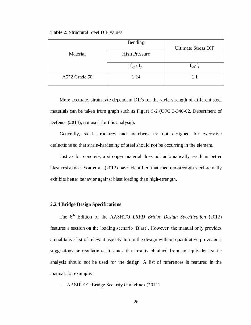


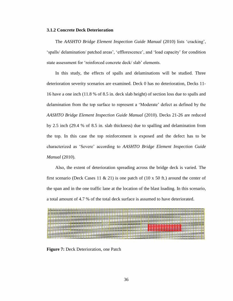
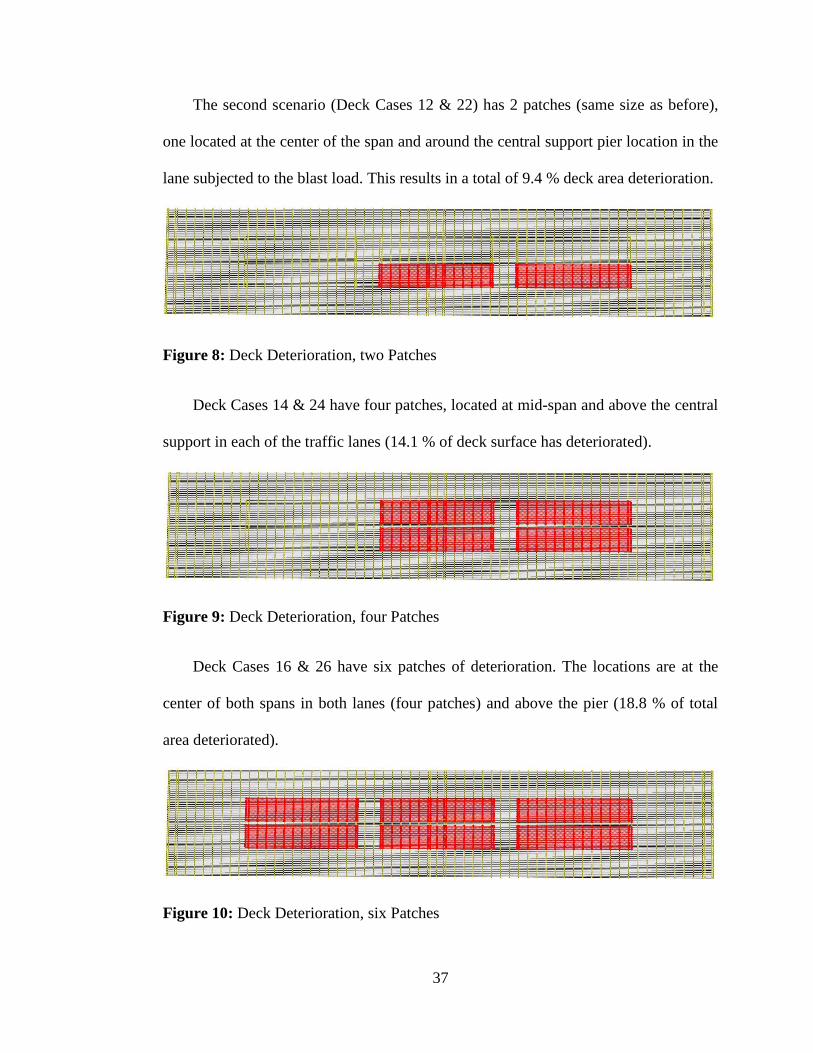

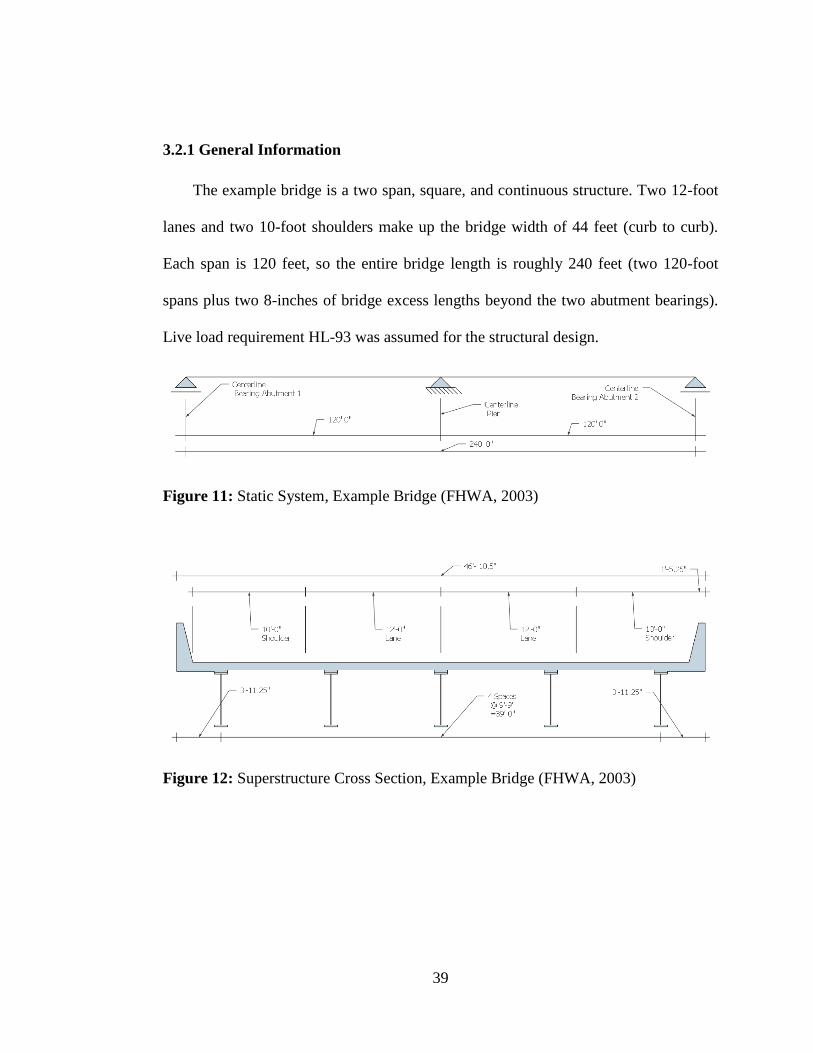


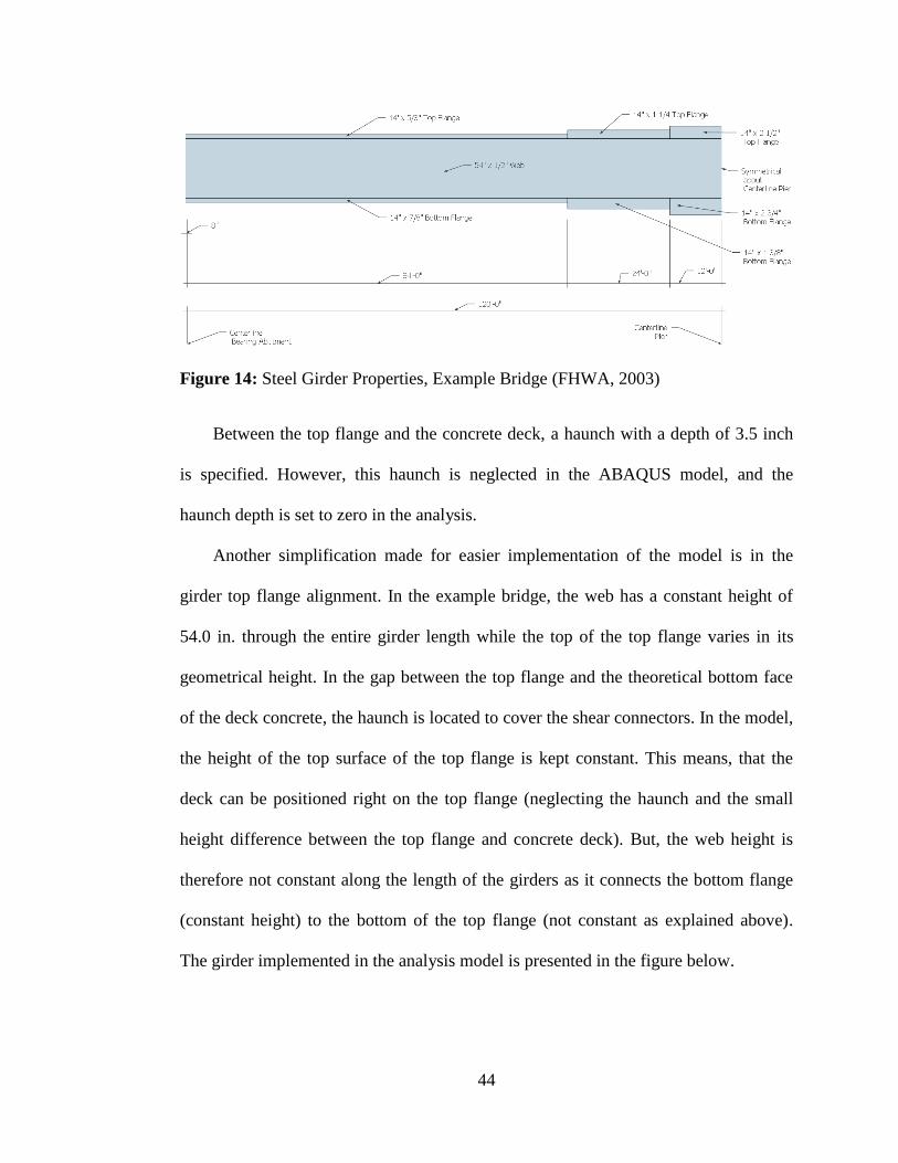
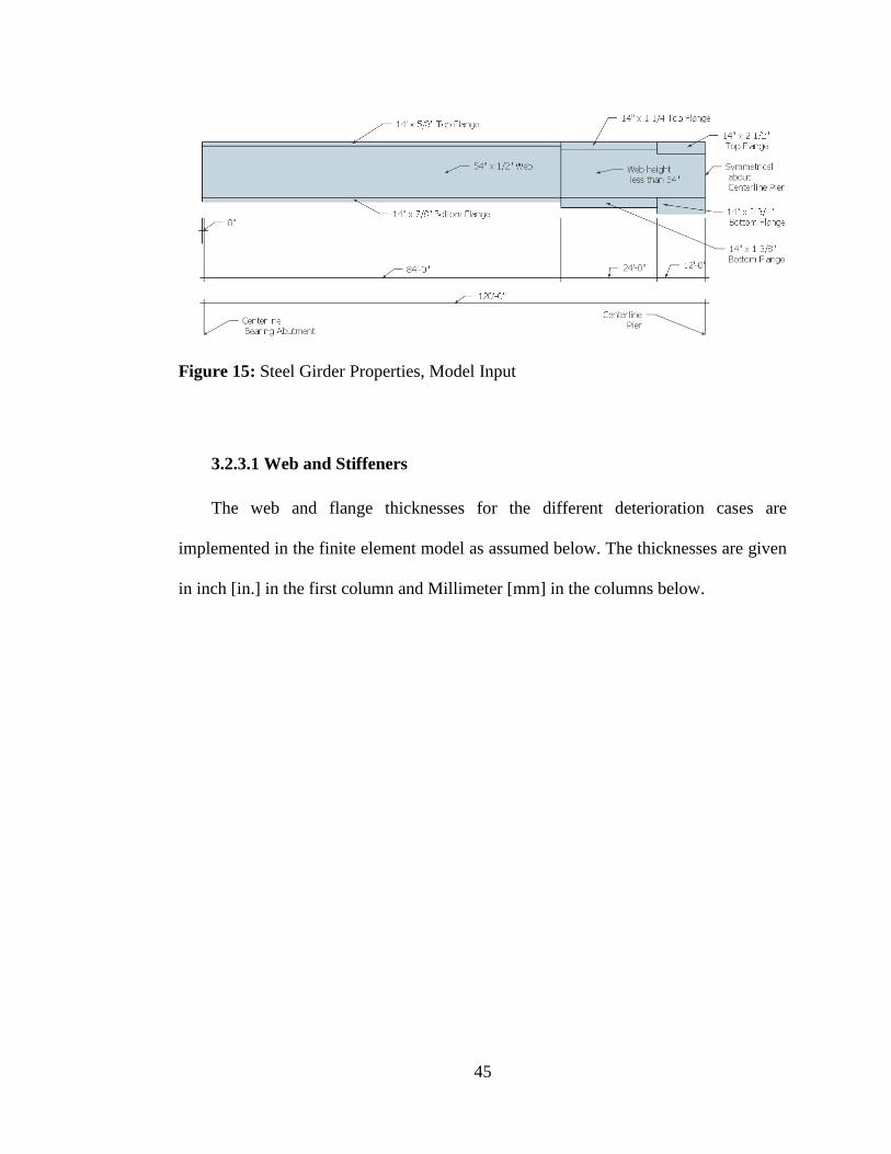

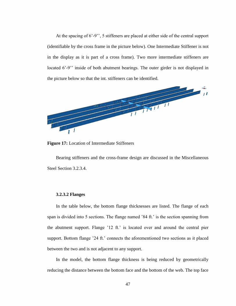


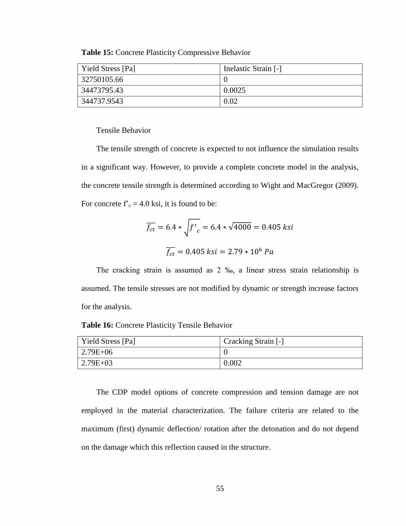


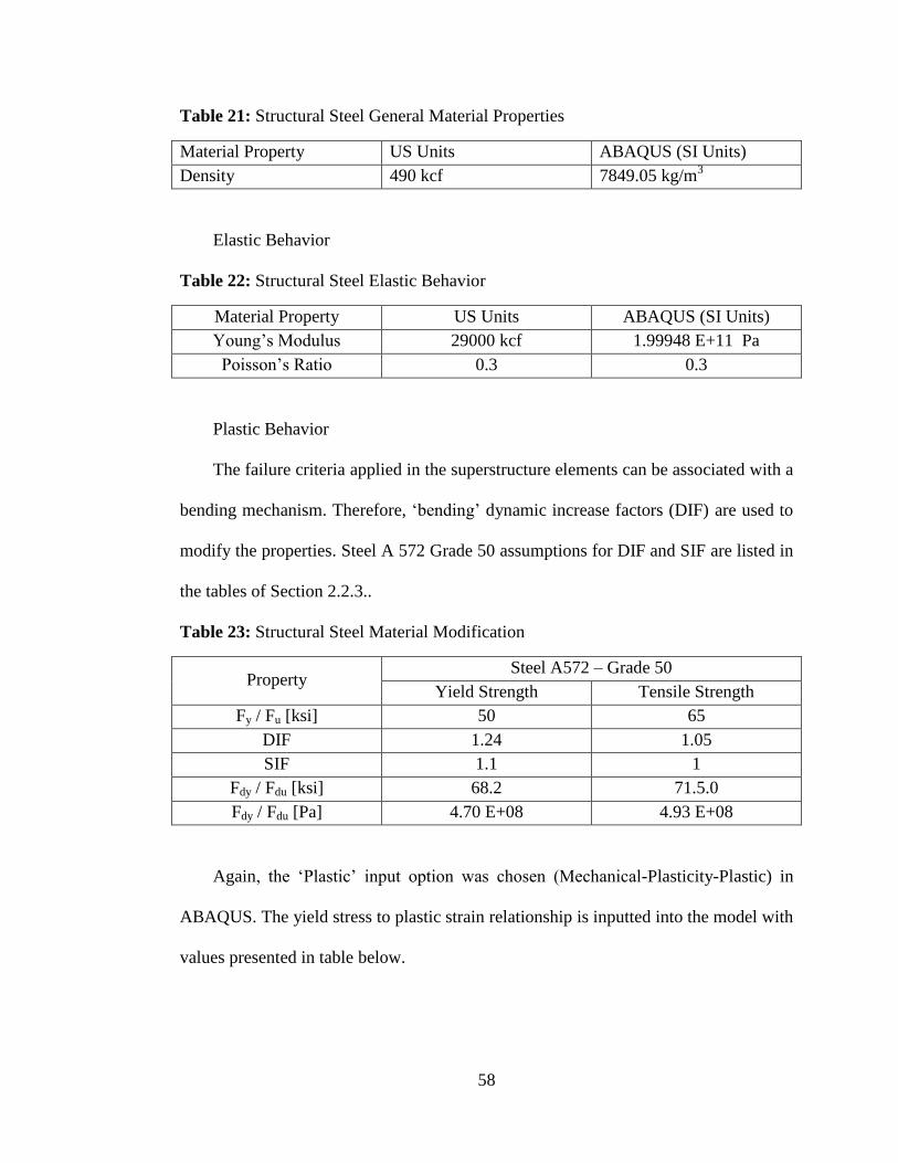
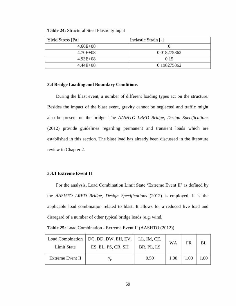
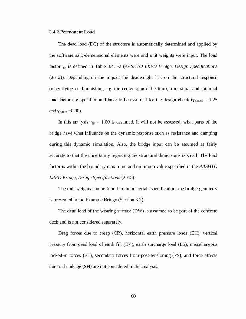


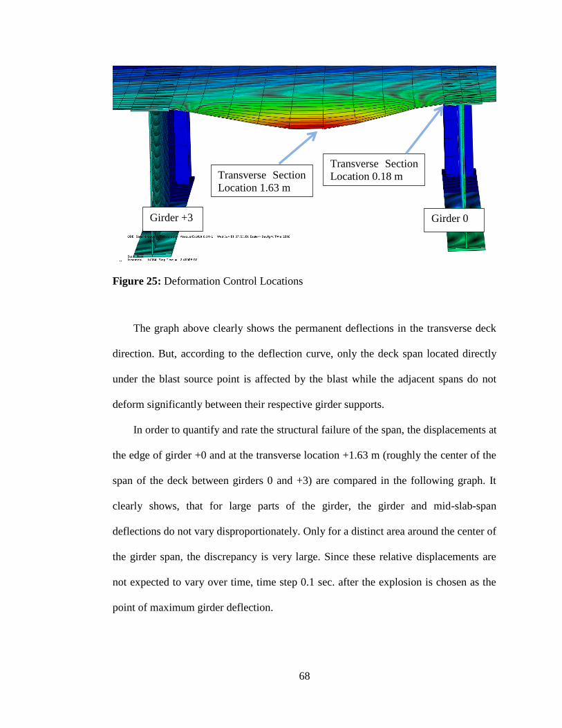

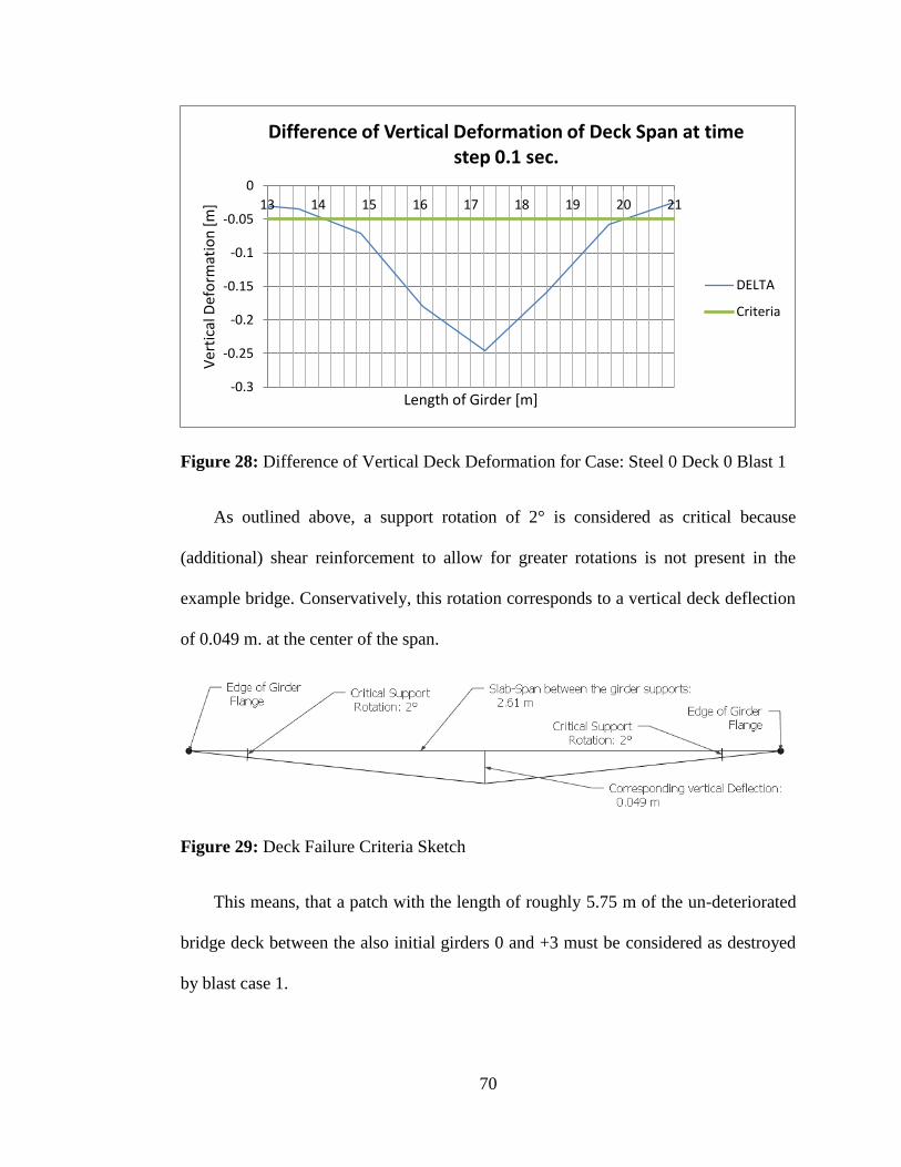

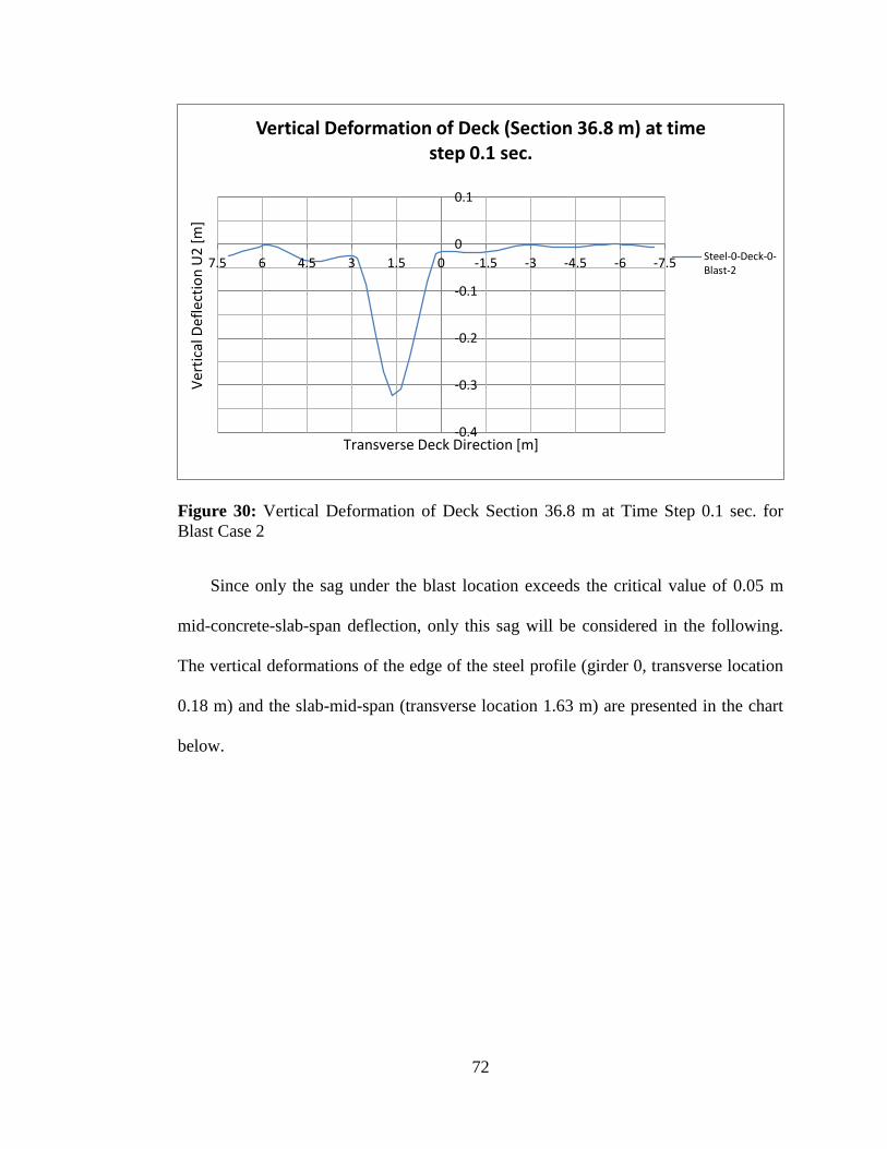
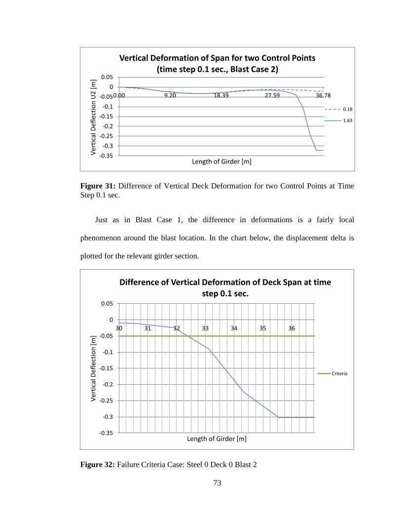
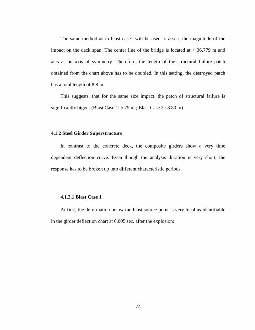


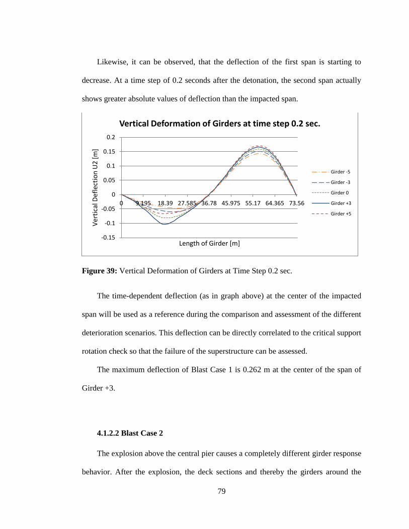


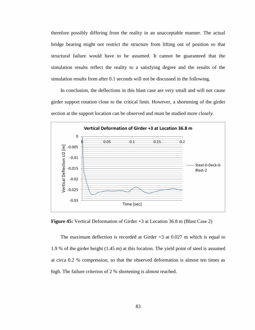
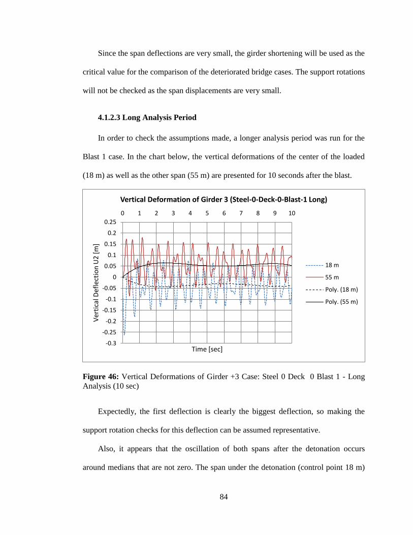


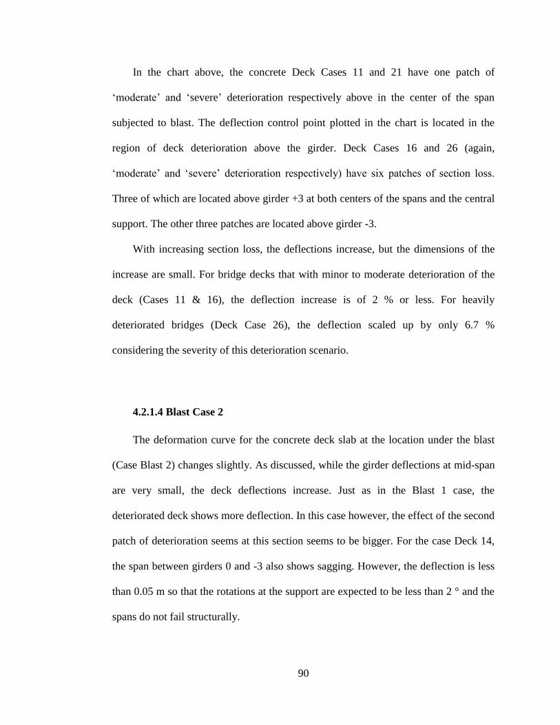
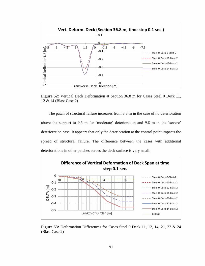

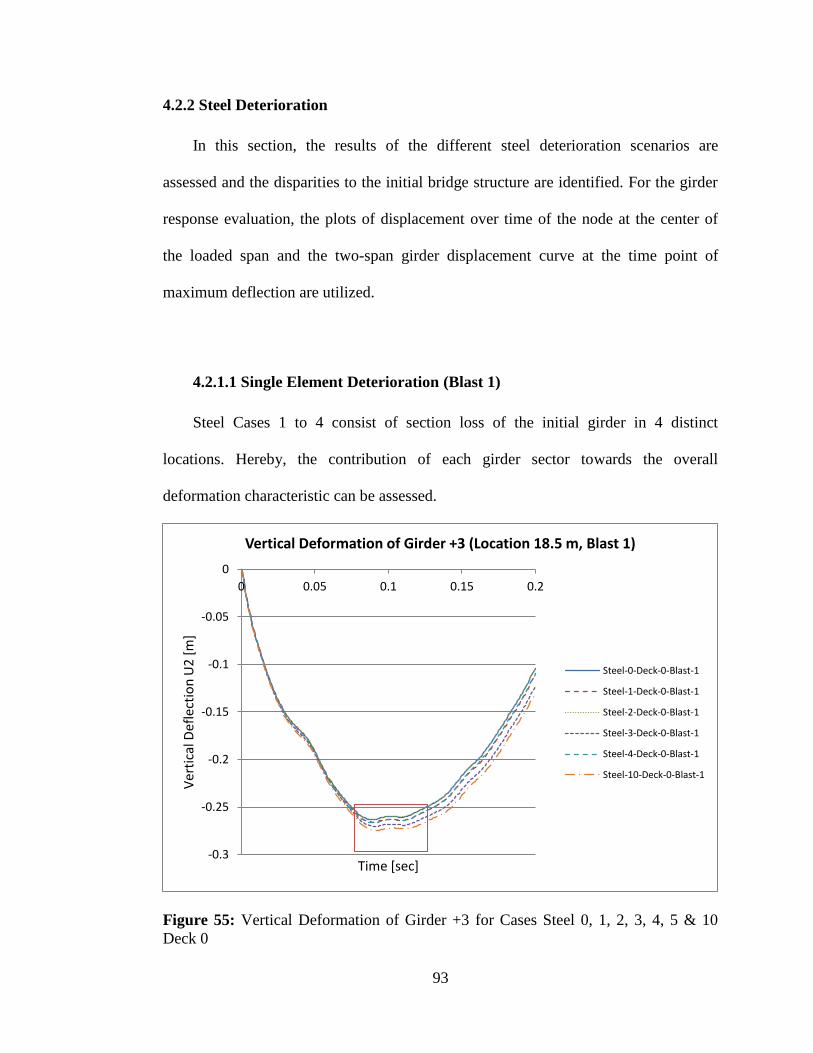
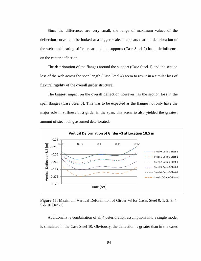
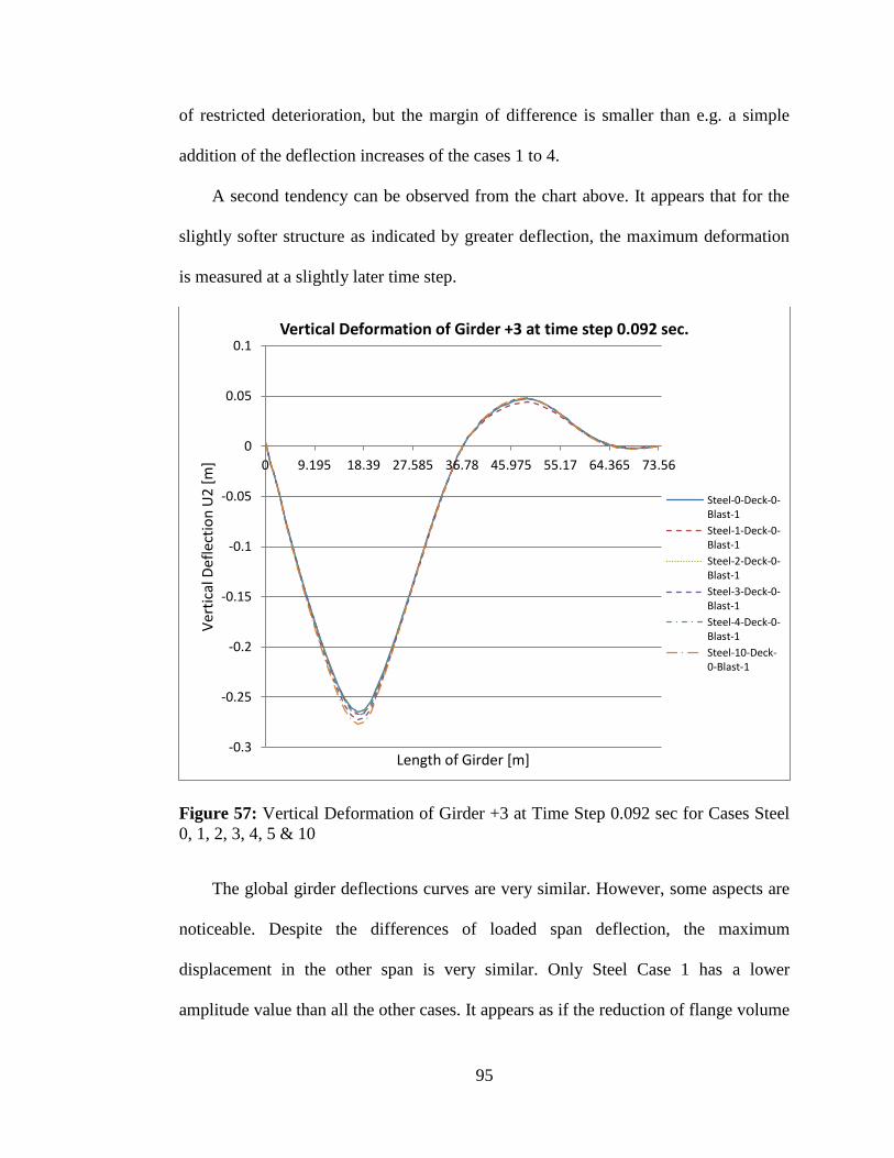
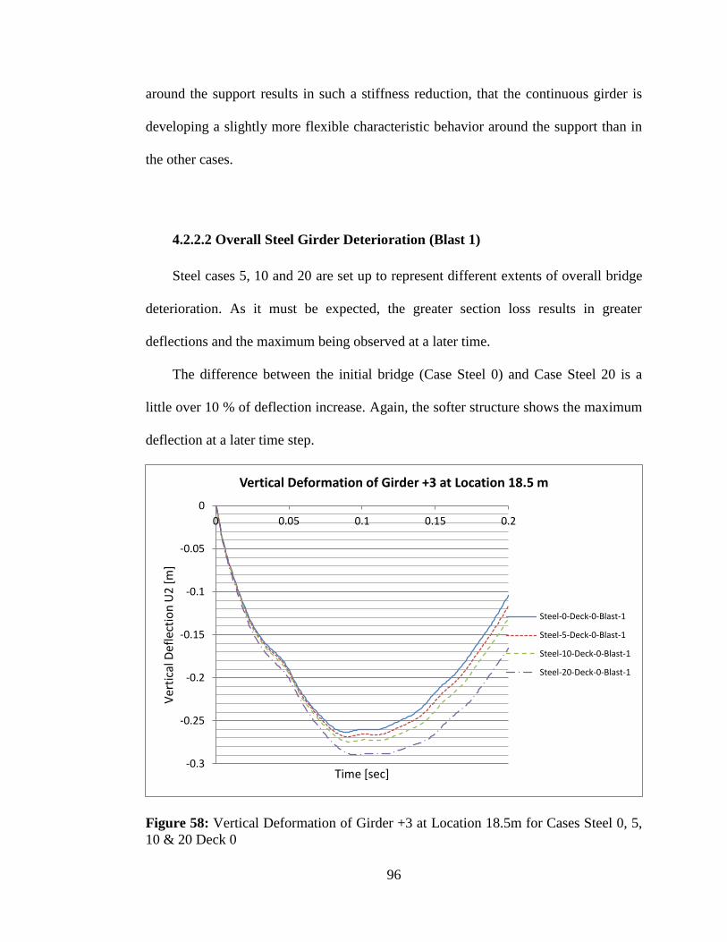


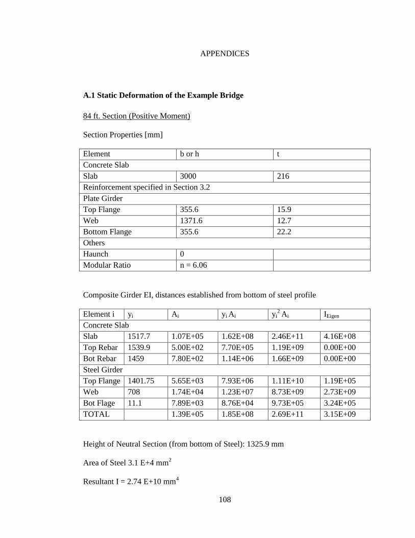


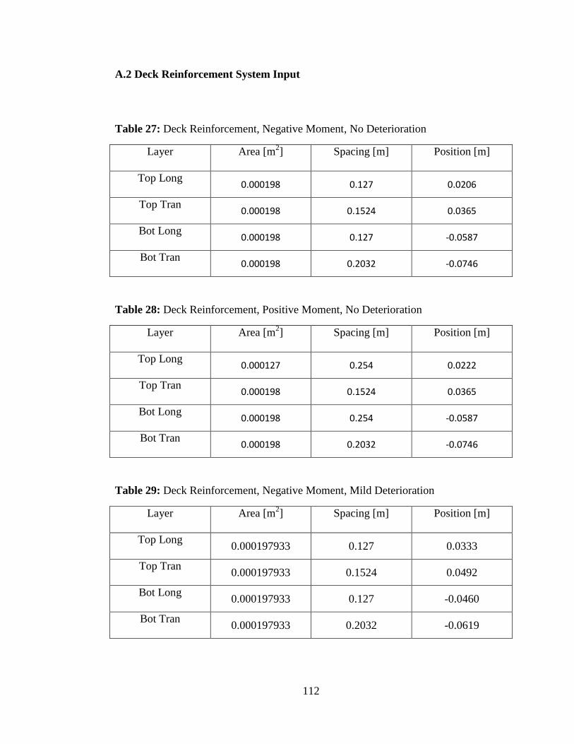
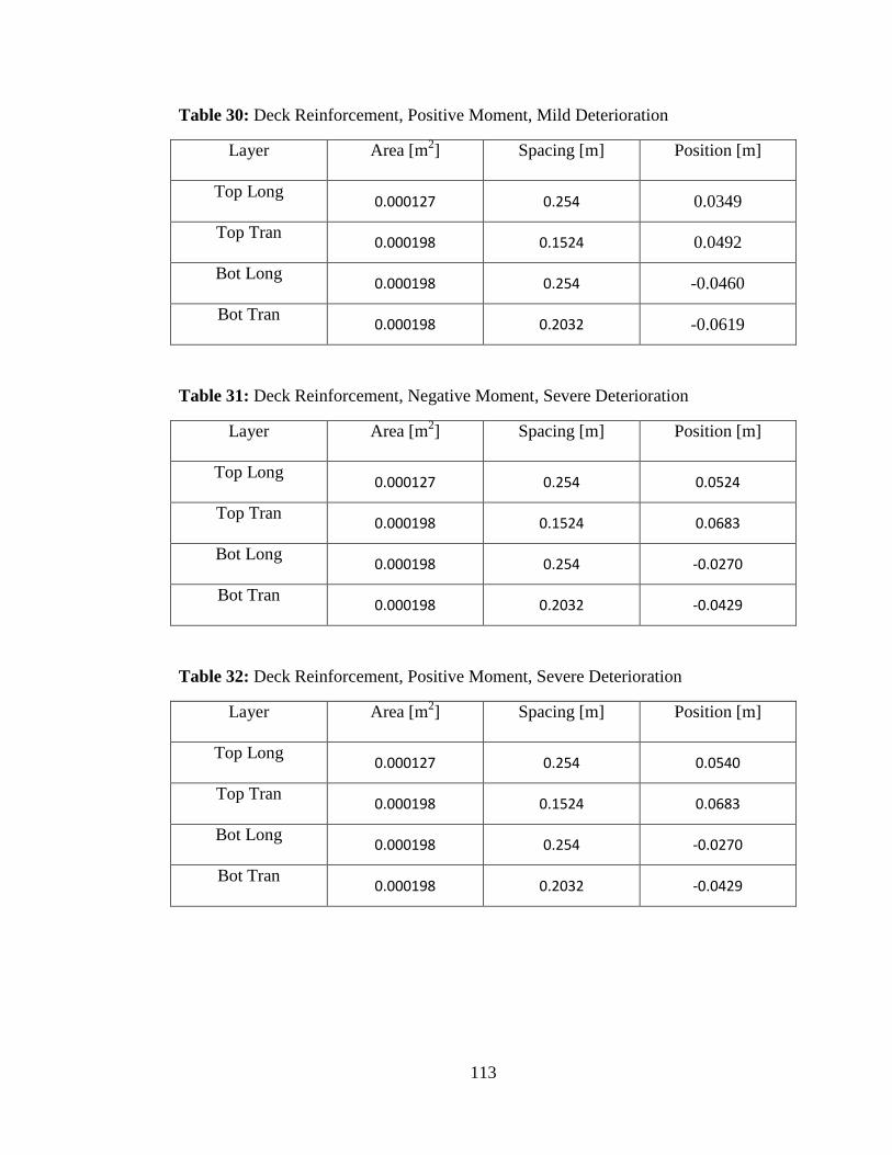


![SOP-T06 Joshua Corman Building Bridges: Surprising ... Bridges: Surprising Strategies and Teammates for Infosec ... Vulnerability Assessment. Multi ... Adversary ROI: [SlideShare]](https://static.documents.pub/doc/80x56/5ab0fc9d7f8b9abc2f8c1bfe/sop-t06-joshua-corman-building-bridges-surprising-bridges-surprising-strategies.jpg)
