70
WATER FOOTPRINT AND VIRTUAL WATER TRADE OF CHINA PAST AND FUTURE L. Z HUO M.M. MEKONNEN A.Y. H OEKSTRA J UNE 2016 V ALUE OF WATER RESEARCH REPORT SERIES NO. 69

WATER FOOTPRINT AND VIRTUAL
WATER TRADE OF CHINA
PAST AND FUTURE
L. ZHUO
M.M. MEKONNEN
A.Y. HOEKSTRA
JUNE 2016
VALUE OF WATER RESEARCH REPORT SERIES NO. 69


WATER FOOTPRINT AND VIRTUAL WATER TRADE OF CHINA: PAST AND FUTURE
L. ZHUO
M. M. MEKONNEN
A. Y. HOEKSTRA*
JUNE 2016
VALUE OF WATER RESEARCH REPORT SERIES NO. 69
Twente Water Centre, University of Twente, Enschede, The Netherlands
* Corresponding author: email [email protected]

© 2016 L. Zhuo, M.M. Mekonnen and A.Y. Hoekstra.
Published by:
UNESCO-IHE Institute for Water Education
P.O. Box 3015
2601 DA Delft
The Netherlands
The Value of Water Research Report Series is published by UNESCO-IHE Institute for Water Education, in
collaboration with University of Twente, Enschede, and Delft University of Technology, Delft.
All rights reserved. No part of this publication may be reproduced, stored in a retrieval system, or transmitted, in
any form or by any means, electronic, mechanical, photocopying, recording or otherwise, without the prior
permission of the authors. Printing the electronic version for personal use is allowed.
Please cite this publication as follows:
Zhuo, L., Mekonnen, M.M. and Hoekstra, A.Y. (2016) Water footprint and virtual water trade of China: Past
and future, Value of Water Research Report Series No. 69, UNESCO-IHE, Delft, the Netherlands.
Acknowledgement This report reproduces an article published in Water Research together with another article published in
Environment International. The work was partially developed within the framework of the Panta Rhei Research
Initiative of the International Association of Hydrological Sciences (IAHS). The data supporting the results can
be achieved through the first author.

Contents
Summary .................................................................................................................................................................. 7
Part 1. Water footprints and inter-regional virtual water flows in China over 1978-2008 ..................................... 9
1. Introduction ...................................................................................................................................................... 9
2. Method and data ............................................................................................................................................. 132.1. Estimating water footprint related to crop consumption ......................................................................... 13
2.2. Estimating water footprint of crop production ........................................................................................ 13
2.3. Estimating inter-regional virtual water flows ......................................................................................... 13
2.4. Quantifying water savings through crop trade ........................................................................................ 14
2.5. Data ......................................................................................................................................................... 15
3. Results ............................................................................................................................................................ 17
3.1. Water footprint of crop consumption ...................................................................................................... 173.2. Water footprint of crop production ......................................................................................................... 19
3.3. Crop-related inter-regional virtual water flows in China ........................................................................ 21
3.4. National water saving related to international and inter-regional crop trade .......................................... 23
3.5. Discussion ............................................................................................................................................... 27
4. Conclusions .................................................................................................................................................... 29
Part 2. Water footprint and virtual water trade scenarios for 2030 and 2050 ........................................................ 31
1. Introduction .................................................................................................................................................... 312. Method and data ............................................................................................................................................. 33
2.1 Scenario set-up ......................................................................................................................................... 33
2.2. Estimating water footprints and virtual water trade ................................................................................ 36
2.3. Data ......................................................................................................................................................... 38
3. Results ............................................................................................................................................................ 39
3.1. Water footprint of crop production ......................................................................................................... 39
3.2. Water footprint of food consumption ...................................................................................................... 43
3.3. National virtual water trade related to crop products .............................................................................. 453.4. Discussion ............................................................................................................................................... 46
4. Conclusion ...................................................................................................................................................... 49
References .............................................................................................................................................................. 51
Appendix I. An example of assessing the water footprint related to crop consumption in China: wheat in the year
2006 ............................................................................................................................................................... 61Appendix II. Relative changes in annual precipitation in China from 2005 to 2050 across GCMs for RCP2.6
(left) and RCP8.5 (right) ................................................................................................................................ 63

Appendix III. Relative changes in annual reference evapotranspiration in China from 2005 to 2050 across
GCMs for RCP2.6 (left) and RCP8.5 (right) ................................................................................................. 64
Appendix IV. Relative changes in national average crop yield in China from 2005-2050 under each scenario .. 65

Summary
The long-term sustainability of human’s water consumption is being challenged by climate change, population
growth, socio-economic development and intensified competition for finite water resources among different
sectors. Previous studies into the relation between human consumption and indirect water resources use have
unveiled the remote connections in virtual water (VW) trade networks, which show how communities
externalize their water footprint (WF) to places far beyond their own region, but little has been done to
understand variability in time. With a focus on crop production, consumption and trade of China, this study
quantifies the inter-annual variability and developments in consumptive (green and blue) WFs and VW trade in
China over the period 1978-2008 (Part 1) and assesses consumptive WFs and VW trade of China under
alternative scenarios for 2030 and 2050 (Part 2). We consider five driving factors of change: climate, harvested
crop area, technology, diet, and population. Evapotranspiration, crop yields and WFs of crops are estimated at a
5×5 arc-minute resolution for 22 crops. Four future scenarios (S1–S4) are constructed by making use of three of
IPCC's shared socio-economic pathways (SSP1–SSP3) and two of IPCC's representative concentration
pathways (RCP 2.6 and RCP 8.5) and taking 2005 as the baseline year.
Results show that, over the period 1978-2008, crop yield improvements helped to reduce the national average
WF of crop consumption per capita by 23%, with a decreasing contribution to the total from cereals and
increasing contribution from oil crops. The total consumptive WFs of national crop consumption and crop
production, however, grew by 6% and 7%, respectively. Historically, the net VW within China was from the
water-rich South to the water-scarce North, but intensifying North-to-South crop trade reversed the net VW flow
since 2000, which amounted 6% of North’s WF of crop production in 2008. China’s domestic inter-regional
VW flows went dominantly from areas with a relatively large to areas with a relatively small blue WF per unit
of crop, which in 2008 resulted in a trade-related blue water loss of 7% of the national total blue WF of crop
production. By 2008, 28% of total water consumption in crop fields in China served the production of crops for
export to other regions and, on average, 35% of the crop-related WF of a Chinese consumer was outside its own
province. Across the four future scenarios and for most crops, the green and blue WFs per tonne will decrease
compared to the baseline year, due to the projected crop yield increase, which is driven by the higher
precipitation and CO2 concentration under the two RCPs and the foreseen uptake of better technology. The WF
per capita related to food consumption decreases in all scenarios. Changing to the less-meat diet can generate a
reduction in the WF of food consumption of 44% by 2050. As a result of the projected increase in crop yields
and thus overall growth in crop production, China will reverse its role from net VW importer to net VW
exporter. However, China will remain a big net VW importer related to soybean, which accounts for 5% of the
WF of Chinese food consumption (in S1) by 2050.
The past of China shows that domestic trade, as governed by economics and governmental policies rather than
by regional differences in water endowments, determines inter-regional water dependencies and may worsen
rather than relieve the water scarcity in a country. All future scenarios show that China could attain a high
degree of food self-sufficiency while simultaneously reducing water consumption in agriculture. However, the
premise of realizing the presented scenarios is smart water and cropland management, effective and coherent
policies on water, agriculture and infrastructure, and, as in scenario S1, a shift to a diet containing less meat.


Part 1. Water footprints and inter-regional virtual water flows in China over 1978-2008*
1. Introduction
Since the beginning of this millennium the body of scientific literature on water footprint (WF) and virtual water
(VW) trade assessment is expanding exponentially, as witnessed by the number of papers published on the topic
in Web of Science. The WF, as a multi-dimensional measure of freshwater used both directly and indirectly by a
producer or a consumer, enables to analyse the link between human consumption and the appropriation of water
to produce the products consumed (Hoekstra, 2013). The consumptive WF of producing a crop includes a green
and blue component, referring to consumption of rainfall and irrigation water respectively, thus enabling the
broadening of perspective on water resources as proposed by Falkenmark and Rockström (2004). The
consumptive WF is distinguished from the degradative WF, the so-called grey WF, which represents the volume
of water required to assimilate pollutants entering freshwater bodies. The WF of human consumption within a
certain geographic area consists of an internal WF, referring to the WF within the area itself for making products
that are consumed within the area, and an external WF, referring to the WF in other areas for making products
imported by and consumed within the geographic area considered (Hoekstra et al., 2011). Thus, trade in water-
intensive commodities like crops results into so-called VW flows between exporting and importing regions
(Hoekstra, 2003). Crop trade saves water resources for an administrative region if it imports water-intensive
crops instead of producing them domestically (Chapagain et al., 2006).
WF and VW trade studies have been carried out for geographies at different scales, from the city (Zhang et al.,
2011) to the globe (Hoekstra and Mekonnen, 2012). Despite the vast body of literature, little attention has been
paid to the annual variability and long-term changes of WFs and VW flows as a result of climate variability and
structural changes in the economy. Most work thus far focussed on employing different models and techniques
to assess WFs and VW flows, considering a specific year or short period of years. The effects of long-term
changes in spatial patterns of production, consumption, trade and climate on WFs and VW flows have hardly
been studied. This is paramount, though, for understanding how human pressure on water resources develops
over time and how changing trade patterns influence inter-regional water dependencies.
The objective of Part 1 of this report is to quantify the effect of inter-annual variability of consumption,
production, trade and climate on crop-related green and blue WFs and inter-regional VW trade, using China
over the period 1978-2008 as a case study. First, we assess the historical development of the green and blue
WFs related to crop consumption in China, per province. Second, we estimate, accounting for the climate
variability within the period considered, the green and blue WFs related to crop production, at a 5×5 arc-minute
resolution, year by year, crop by crop. Third, we quantify the annual inter-regional VW flows based on
provincial crop trade balances for each crop. Finally, we estimate national water savings as a result of
international and inter-regional crop trade. We consider twenty-two primary crops (Table 3), which covered 83%
* This part of the report is based on: Zhuo, L., Mekonnen, M.M. and Hoekstra, A.Y. (2016) The effect of inter-annual variability of consumption, production, trade and climate on crop-related green and blue water footprints and inter-regional virtual water trade: A study for China (1978-2008), Water Research, 94: 73–85.

10 / Water footprint and virtual water trade of China
of national crop harvested area in 2009 (NBSC, 2013) and 97% and 78% of the total blue and green WF of
Chinese crop production in the period 1996-2005, respectively (Mekonnen and Hoekstra, 2011). In this study
we exclude the grey WF of crops because of our focus on inter-annual variability and the fact that variability in
climate plays a role particularly in estimating green and blue WFs, not in estimating grey WFs. We focus on the
direct green and blue WF of crop growing in the field, thus excluding the indirect WF of other inputs into crop
production, like the WF of machineries and energy used. The study area is Mainland China, which consists of
31 provinces and can be grouped into eight regions (Fig. 1).
Figure 1. Provinces and regions of Mainland China.
China is facing severe water scarcity (Jiang, 2009; 2015). Since the economic reforms in 1978, the Chinese
people consume increasing levels of oil crops, sugar crops, vegetables and fruits (Liu and Savenije, 2008).
Chinese crop consumption per capita rose by a factor 2.1 over the period 1978-2008 (FAO, 2014), while
China’s population grew from 0.96 to 1.31 billion (NBSC, 2013). In order to meet the increasing food demand,
China’s crop production grew by a factor 2.8 from 1978 to 2008 (FAO, 2014), with an increase of only 4% in
total harvested area, but a 31% growth in irrigated area. The expansion of the irrigated area occurred mainly
(77%) in the water-scarce North, which now has 51% of the national arable land, but only 19% of the national
blue water resources (Wu et al., 2010; Zhang et al., 2009). Agriculture is the biggest water user in China,
responsible for 63% of national total blue water withdrawals (MWR, 2014) and 88% of the total WF within
China (Hoekstra and Mekonnen, 2012). Currently, the Yellow River basin in the North suffers moderate to
severe blue water scarcity during seven months of the year, mostly driven by agricultural water use (Zhuo et al.,
2016a). The Yongding He Basin in northern China, a densely populated basin serving water to Beijing, faces
severe water scarcity all year long (Hoekstra et al., 2012). It is estimated that about 64% of China’s total
population, mainly from the North, regularly faces severe blue water scarcity (Mekonnen and Hoekstra, 2016).
The competition between different sectors over water resources has become severe (Zhu et al., 2013), which has
Water footprint and virtual water trade of China / 11
led to the adoption of the No. 1 Document by the State Council of China (SCPRC, 2010), announcing a four
trillion CNY (~US$600 billion) investment over ten years to guarantee water supplies through the improvement
of water supply infrastructure. This includes the construction of new reservoirs, drilling of wells, and
implementation of inter-basin water transfer projects (Gong et al., 2011; Yu, 2011), as well as targets to increase
water productivity.
Today, China is the country with the largest WF related to crop consumption and the second largest WF related
to crop production (Hoekstra and Mekonnen, 2012). Furthermore, China has substantive VW import through
crop imports (Dalin et al., 2014). At present, net VW trade through crop trade is from the drier North to the
wetter South (Ma et al., 2006; Cao et al., 2011). In 2005, China’s domestic food trade resulted in national net
water saving overall, but a net loss of blue water (Dalin et al., 2014), as a result of differences in WF of crops
(m3 t-1) among trading provinces (Mekonnen and Hoekstra, 2011).
There have been quite a number of previous studies on the WF of Chinese crop consumption (Hoekstra and
Chapagain, 2007, 2008; Liu and Savenije, 2008; Mekonnen and Hoekstra, 2011; Ge et al. 2011; Hoekstra and
Mekonnen, 2012; Cao et al., 2015), the WF of Chinese crop production (Hoekstra and Chapagain, 2007, 2008;
Siebert and Döll, 2010; Liu and Yang, 2010; Fader et al., 2010; Mekonnen and Hoekstra, 2011; Ge et al. 2011;
Cao et al., 2014a,b), on China’s international VW imports and exports associated with crop trade (Hoekstra and
Hung, 2005; Hoekstra and Chapagain, 2007, 2008; Liu et al., 2007; Fader et al., 2011; Hoekstra and Mekonnen,
2012; Dalin et al., 2012; Chen and Chen, 2013; Shi et al., 2014) and on VW flows within China (Ma et al., 2006;
Guan and Hubacek, 2007; Wu et al., 2010; Cao et al., 2011; Han and Sun, 2013; Sun et al., 2013; Dalin et al.,
2014; Feng et al., 2014; Wang et al., 2014; Zhang and Anadon, 2014; Zhao and Chen, 2014; Fang and Chen,
2015; Jiang et al., 2015; Zhao et al., 2015). Despite all those studies, analyses of inter-annual variability and
long-term changes in spatial WF and VW trade patterns are rare, not only in studies for China but in general.
While in another paper (Zhuo et al., 2016a) we show the inter-annual variations in WFs of crop production as
well as inter-annual variation of blue water scarcity (with a focus on the Yellow River basin), in the current
study we also consider inter-annual variability in WFs of crop consumption and in inter-regional and
international VW trade (for China as a whole).

2. Method and data
2.1. Estimating water footprint related to crop consumption
The annual green and blue WFs of crop consumption (in m3 y-1) were estimated per crop per year at provincial level
based on the bottom-up approach (Hoekstra et al., 2011). The WF related to consumption of a crop (m3 y-1) was
calculated per year by multiplying the provincial crop consumption volume (t y-1) with the WF of the crop for the
province (m3 t-1). Crop consumption volumes per capita were obtained from the Supply and Utilization Accounts
expressed in crops primary equivalent of FAO (2014). We assumed consumption per capita data the same for all
provinces. For edible crops, we took the sum of the “food” and “food manufactured” columns and added an amount
representing seed and waste. Regarding the latter amount, we took a part of the utilization for seed and waste based on
the utilization of crops for food and food manufactured relative to the utilization of crops for feed. For cotton and tobacco,
we took the “other use” column as consumed quantities. The WF of crops per province were calculated as:
(1)
in which Pprov[p] (t y-1) represents the production quantity of crop p, Ie[p] (t y-1) the imported quantity of crop p from
exporting place e (other regions in China or other countries), WFprod,prov[p] (m3 t-1) the specific WF of crop production in
the province, and WFprod,e[p] (m3 t-1) the WF of the crop as produced in exporting place e. An example of WF estimation
related to crop consumption is provided for wheat in the year 2006 in Appendix I.
2.2. Estimating water footprint of crop production
The green and blue WFs of crop production were estimated year by year at 5×5 arc minute resolution. The green and
blue WF (in m3 t-1) of a crop within a grid cell is calculated as the actual green and blue evapotranspiration (ET, m3 ha-1)
over the growing period divided by the crop yield (Y, t ha-1). ET and Y were simulated per crop per grid per year at daily
basis using the plug-in version of FAO’s crop water productivity model AquaCrop version 4.0 (Steduto et al, 2009; Reas
et al., 2009; Hsiao et al., 2009). The separation of green and blue ET was carried out by tracking the daily green and blue
soil water balances based on the contribution of rainfall and irrigation, respectively, following Chukalla et al. (2015) and
Zhuo et al. (2016a).
2.3. Estimating inter-regional virtual water flows
Inter-regional VW flows (m3 y-1) related to crop trade were calculated per year by multiplying the inter-regional crop
trade flows (t y-1) with the WF of the crop (m3 t-1) in the exporting region. Since inter-regional crop trade statistics are not
available, we took the following steps:
1) The provincial crop trade balance or net import of a crop (t y-1) was estimated as the total provincial crop utilization
minus the provincial crop production. The national use of a crop for direct and manufactured food as given by FAO
(2014) was distributed over the provinces based on provincial populations. The national use of a crop for feed was
prov prod,prov e prod,ee
provprov e
e
P [ ] WF [ ] (I [ ] WF [ ])WF [ ] =
P [ ] I [ ]
p p p pp
p p
× + ×
+
∑∑

14 / Water footprint and virtual water trade of China
distributed over provinces proportional to the national livestock units (LU) per province. LU is a reference unit
which facilitates the aggregation of different livestock types to a common unit, via the use of a ‘livestock unit
coefficient’ obtained by converting the livestock body weight into the metabolic weight by an exchange ratio (FAO,
2005). We used the livestock unit coefficients for East Asia from Chilonda and Otte (2006): 0.65 for cattle, 0.1 for
sheep and goats, 0.25 for pigs, 0.5 for asses, 0.65 for horses, 0.6 for mules, 0.8 for camels, and 0.01 for chickens.
Finally, we downscale national variations in crop stock to provincial level by assuming provincial stock variations
proportional to the provincial share in national production.
2) We assume that international crop imports and exports relate to the provinces with deficit and surplus of the crop,
respectively (following Ma et al., 2006). Further we assume that crop-deficit provinces primarily receive from crop-
surplus provinces within the same region and subsequently – if insufficient surplus within the region itself – from
other crop-surplus regions.
3) A crop-deficit region is assumed to import the crop preferentially from the crop-surplus region which has the highest
agricultural export values to the crop-deficit region, according to the multi-regional input-output tables of the
agricultural sector for the years 1997 (SIC, 2005), 2002 and 2007 (Zhang and Qi, 2011). How source regions supply
deficit regions is determined in a few subsequent rounds. The source regions per region per allocation round are
listed in Table 1. We assume that in each round the crop source regions supply crops to the deficit regions
proportionally to their deficit.
Table 1. Crop source regions per region for Mainland China.
Region* Provinces Crop source regions per allocation round
1 2 3 4 5 6 7
R1 Northeast (N) Heilongjiang, Jilin, Liaoning R3 R7 R6 R8 R5 R4 R2
R2 Jing-Jin (N) Beijing, Tianjin R3 R7 R1 R6 R8 R5 R4
R3 North Coast (N) Hebei, Shandong R7 R1 R6 R8 R2 R5 R4
R4 East Coast (S) Jiangsu, Shanghai, Zhejiang R6 R7 R3 R1 R8 R5 R2
R5 South Coast (S) Fujian, Guangdong, Hainan R6 R8 R7 R3 R1 R4 R2
R6 Central Shanxi (N), Henan (N), Anhui (N), Hubei (S), Hunan (S), Jiangxi (S) R3 R7 R1 R8 R5 R4 R2
R7 Northwest (N) Inner Mongolia, Shaanxi, Ningxia, Gansu, Qinghai, Xinjiang R6 R3 R8 R1 R5 R4 R2
R8 Southwest (S) Sichuan, Chongqing, Guangxi, Yunnan, Guizhou, Tibet R7 R1 R6 R3 R5 R4 R2
* N = North China; S = South China.
The total crop-related net VW import (m3 y-1) of a province is equal to the international net VW import plus the inter-
regional net VW import of the province. The WFs (m3 t-1) of crops imported from abroad were obtained from Mekonnen
and Hoekstra (2011), assuming constant green and blue WFs of imported crops per source country. The provincial net
VW export related to a certain crop export is calculated by multiplying the net crop export volume (t y-1) with the WF
(m3 t-1) of the crop in the province.

Water footprint and virtual water trade of China / 15
2.4. Quantifying water savings through crop trade
Water savings through crop trade were estimated using the method of Chapagain et al. (2006). The international crop
trade-related water saving of a province (m3 y-1) was calculated by multiplying the net international import volume of the
province (t y-1) by the WF per tonne of the crop in the province (m3 t-1). The inter-regional crop trade-related water
saving was estimated similarly, by multiplying the net inter-regional import volume of the province (t y-1) with the WF
per tonne of the crop in the province (m3 t-1). If a specific crop is imported and not grown in the province itself at all, the
national average WF per tonne of the crop was used. Overall trade-related water savings follow from the difference in the
WF of a crop in the importing and exporting province (Hoekstra et al., 2011). When calculated trade-related water
savings are negative, we talk about trade-related ‘water losses’, which refer to cases whereby crops are traded from a
region with relatively low water productivity to a region with relatively high water productivity.
2.5. Data
The GIS polygon for Chinese provinces was obtained from NASMG (2010). Provincial population statistics over the
study period and numbers of the different livestock types were obtained from NBSC (2013), and data on China’s
international trade per crop (in t y-1) from FAO (2014). Data on monthly precipitation, reference evapotranspiration and
temperature at 30×30 arc minute resolution were taken from Harris et al. (2014). Figure 2 shows the inter-annual
variation of national average precipitation and reference evapotranspiration (ET0) across China over the period 1978-
2008. Data on irrigated and rain-fed areas for each crop at 5×5 arc-minute resolution were taken from Portmann et al.
(2010). For crops not available in this source, we used Monfreda et al. (2008). Harvested areas and yields for each crop
were scaled per year to fit the annual agriculture statistics at province level obtained from NBSC (2013). For crops not
reported in NBSC (2013), we used FAO (2014). Soil texture data were obtained from Dijkshoorn et al. (2008). For
hydraulic characteristics for each type of soil, the indicative values provided by AquaCrop were used. Data on total soil
water capacity were obtained from Batjes (2012). Details on datasets used can be found in Table 2.
Figure 2. Inter-annual variation of national average precipitation and reference evapotranspiration (ET0) across China over
the period 1978-2008. Data source: Harris et al. (2014).

16 / Water footprint and virtual water trade of China
Table 2. Overview of data sources.
Data type Spatial resolution Source(s)
GIS database of administrations Provincial NASMG (2010)
Annual population statistics Provincial NBSC (2013)
Statistics on annual total production and total
harvested area of each crop Provincial/national NBSC (2013) / FAO (2014)
Statistics on crop trade International FAO (2014)
Monthly climate data on precipitation and ET0 30×30 arc minute Harris et al., 2014
Irrigated and rain-fed area of each crop 5×5 arc minute Portmann et al., 2010) / Monfreda et al. (2008)
Soil texture 1 : 1,000,000 Dijkshoorn et al. (2008)
Total soil water capacity 5×5 arc minute Batjes (2012)

Water footprint and virtual water trade of China / 17
3. Results
3.1. Water footprint of crop consumption
Over the study period 1978-2008, Chinese annual per capita consumption of the 22 considered crops has grown by a
factor 1.4, from 391 to 559 kg cap-1. The national average WF per capita related to crop consumption reduced by 23%,
from 625 m3 cap-1 (149 m3 cap-1 blue WF) in 1978 to 481 m3 cap-1 (94 m3 cap-1 blue WF) in 2008 (Fig. 3), which was
mainly due to the decline in the WF per tonne of crops (Table 3). The decline in the WF per tonne of crop resulted from
improved crop yields within China as well as the expanded international import of crops from other countries with
relatively small WF. The share of the WF related to the consumption of oil crops (soybean, groundnuts, sunflower and
rapeseed) in the total consumptive WF per capita grew from 8% in 1978 to 21% in 2008 (Fig. 3), as a result of the
increased proportion of oil crops in Chinese consumption.
Figure 3. National average water footprint per capita (m3 cap-1 y-1) related to crop consumption in China, specified by water
footprint colour (upper graph) and by crop group (lower graph). Period: 1978-2008. The figures represent crop
consumption for food, thus excluding crop consumption for feed.
Due to differences in the WF (in m3 t-1) of the consumed crops in the different provinces, there were differences among
provinces in terms of WFs per capita, ranging from 367 to 604 m3 cap-1 y-1 for the total consumptive WF and from 29 to
228 m3 cap-1 y-1 for the blue WF in the year 2008. Fourteen provinces, mostly located in Southwest, Northeast, North
Coast and East Coast, have a WF per capita below the national average (Fig. 4). The three provinces with the largest WF

18 / Water footprint and virtual water trade of China
per capita related to crop consumption in 2008 were Ningxia (604 m3 cap-1 y-1), Guangxi (587 m3 cap-1 y-1) and
Guangdong (586 m3 cap-1 y-1). Chongqing had the smallest WF per capita (367 m3 cap-1 y-1). Provinces with a blue WF
per capita smaller than the national average are mostly located in Southwest, Northeast and East Coast. The three
provinces with the largest blue WF per capita in 2008 are all located in the semi-arid Northwest: Inner Mongolia (228 m3
cap-1 y-1), Xinjiang (214 m3 cap-1 y-1) and Ningxia (213 m3 cap-1 y-1). Anhui had the smallest blue WF per capita (29 m3
cap-1 y-1).
Although the total consumption of the 22 considered crops doubled between 1978 and 2008, with 37% of population
growth in China, the national WF related to crop consumption increased only by 6%, from 599 to 632 billion m3 y-1 (Fig.
5), thanks to the decline in the WF of crops (m3 t-1). The share of North China in the total national consumptive WF of
crop consumption decreased from 48 to 44% over the study period, amongst other driven by the slightly faster population
growth in the South. At provincial level, Shanghai had the largest increase in the WF of crop consumption, a 2.3 times
increase over the study period (from 4.6 to 10.5 billion m3 y-1), followed by Beijing with a 2.0 times increase (from 4.4 to
8.6 billion m3 y-1). This was mainly driven by the doubling of the population in these two megacities (from 11.0 to 21.4
million in Shanghai and from 8.7 to 17.7 million in Beijing).
Figure 4. China’s provincial average total and blue water footprints per capita (m3 cap-1 y-1) related to crop consumption in
2008. The figures refer to crop consumption for food, thus excluding crop consumption for feed.
Figure 5. Consumptive water footprints (WFs) of crop consumption in China (left), and the relative contributions of North
and South China to the total (right). The figures refer to crop consumption for food, thus excluding crop consumption for feed.

Water footprint and virtual water trade of China / 19
Table 3. National average water footprint of crops consumed in China for the years 1978 and 2008.
1978 2008
Green WF Blue WF Total WF Green WF Blue WF Total WF
m3 t-1 m3 t-1 m3 t-1 m3 t-1 m3 t-1 m3 t-1
Wheat 2080 817 2897 839 312 1151
Maize 1412 121 1534 754 66 819
Rice 1486 615 2101 961 384 1345
Sorghum 1080 88 1168 714 45 759
Barley 839 558 1397 832 198 1030
Millet 2042 184 2225 1811 133 1945
Potatoes 264 7 271 189 7 196
Sweet potatoes 74 40 114 67 21 88
Soybean 3718 677 4395 2024 110 2134
Groundnuts 3165 395 3560 1345 191 1536
Sunflower seed 2177 289 2466 1087 184 1270
Rapeseed 4292 0 4292 1736 0 1736
Seed cotton 5093 539 5632 1278 503 1781
Sugar cane 208 3 211 120 1 121
Sugar beet 372 0 372 66 0 66
Spinach 100 8 107 79 4 83
Tomatoes 126 3 129 68 2 70
Cabbages 181 15 196 130 7 137
Apples 1367 157 1524 314 39 353
Grapes 1011 304 1314 316 104 421
Tea 33518 226 33744 8517 144 8662
Tobacco 2381 84 2465 1633 13 1646
National averages are calculated weighing the water footprints of domestically produced and imported crops.
3.2. Water footprint of crop production
The total green plus blue WF in China of producing the 22 crops considered increased over the period 1978-2008 by 7%,
from 682 billion m3 y-1 (23% of blue) to 730 billion m3 y-1 (19% of blue) (Fig. 6), while total production of those crops
grew by a factor 2.2. The relatively modest growth of the WF can be attributed to a significant decrease in the WFs per
tonne of crop, which in turn result from an increase in crops yield. The national average WF of cereals (wheat, rice,
maize, sorghum, millet, and barley), for example, decreased by 46%, from 2136 m3 t-1 (540 m3 t-1 blue WF) to 1146 m3 t-1
(249 m3 t-1 blue WF), due to an almost two-fold increase in cereal yield (from 2.9 to 5.6 t ha-1) (Fig. 7). These findings
correspond to long-term decreases in WFs per tonne found in a case study for the Yellow River basin by Zhuo et al.
(2016a). Inter-annual climatic variability contributed to the fluctuations in consumptive WFs (m3 t-1) over the years.
When comparing the fluctuations in the average green and blue WFs of a cereal crop in China over the period 1978-2008
(as shown in Fig. 7) to the variations in annual precipitation and ET0 over the same period (Fig. 2), we find that the blue
WF inversely relates to precipitation, and that the green and total consumptive WFs show a weak positive relation to ET0.

20 / Water footprint and virtual water trade of China
In years with relatively large precipitation, the ratio of blue to total consumptive WF is generally smaller, a finding that
could be expected because irrigation requirements will generally be less.
The total harvested area of the considered crops increased by 16% in the North and decreased by 13% in the South. The
harvested area and the total consumptive WF of crop production decreased in the provinces that have relatively high
urbanization levels (Beijing, Tianjin, Shanghai, Chongqing, Zhejiang, Fujian, Hubei, and Guangdong) and are mostly
located in the water-rich South. The most significant drop in the total consumptive WF of crop production (a 65%
decrease) was in Shanghai and Zhejiang, with halved harvested areas. At the same time, the other provinces mostly
located in the water-scarce North, experienced increases in the total consumptive WF of crop production. The most
significant increase (fivefold) in the total consumptive WF was observed in Inner Mongolia, which is located in the semi-
arid Northwest, where the harvested area expanded by a factor 3.5 and the irrigated area by a factor 2. The contribution
of the water-scarce North to the WF of national crop production increased from 43% in 1978 to 51% in 2008 as a result
of increasing cropping area in the North compared to the South and increased irrigation in the North (Fig. 6).
Figure 6. Consumptive water footprints (WFs) of crop production in China, and the relative contributions of North and
South China.
Figure 7. Green and blue WF of cereals (m3 t-1) and cereal yield (t ha-1) in China.

Water footprint and virtual water trade of China / 21
Figure 8 shows the spatial distribution of the total consumptive WF (in mm y-1) of crop production, as well as the share of
blue in the total, averaged over the period 1999-2008. Large total consumptive WFs correlate with large overall
harvested areas and/or the production of relatively water-intensive crops, while a large share of blue WF in the total
reflects the presence of intensive irrigated agriculture. In the semi-arid Northwest and North Coast, blue WF shares
exceed 40%, with Xinjiang having the highest share (54%), followed by Hebei (43%) and Ningxia (35%).
Cereals (wheat, maize, rice, sorghum, millet and barley) accounted for 74% of the overall consumptive WF of the 22 crops
considered, 87% of the blue WF, and 71% of the green WF. More than half of the total blue WF within China was from rice
fields (51%), followed by wheat (28%). Rice (32%) and wheat (20%) together also shared half of the total green WF.
Figure 8. Spatial distribution of consumptive water footprints (WFs) (mm y-1) of crop production (left) and the share of the
blue WF in the total (right) in China.
3.3. Crop-related inter-regional virtual water flows in China
China’s annual net VW import from abroad nearly tripled over the period 1978-2008 (from 34 to 95 billion m3 y-1). The
external WF related to crop consumption in China as a whole was 6% of the total in 1978 and 13% in 2008. The inter-
regional VW flows within China were larger than the country’s international VW flow. The sum of China’s inter-
regional VW flows was relatively constant over the period 1978-2000 (with an average of 187 billion m3 y-1), and rose to
a bit higher level during the period 2001-2008 (average 207 billion m3 y-1) (Fig. 9). With a total consumptive WF of
Chinese crop production in 2008 of 730 billion m3 y-1 and a total gross inter-regional VW trade of 207 billion m3 y-1, we
find that 28% of total water consumption in crop fields in China serves the production of crops for export to other regions.
When we consider blue water consumption specifically, we find the same value of 28%. Further we find that, on average,
in 2008, 35% of the crop-related WF of a Chinese consumer is outside its own province. For some provinces we find
much larger external WFs in 2008: 92% for Tibet (83% in other provinces, 10% abroad), 88% for Beijing (68% in other
provinces, 20% abroad) and 86% for Shanghai (66% in other provinces, 20% abroad).
The estimated inter-regional trade of the crops considered increased by a factor 2.3 over the study period, but the sum of
inter-regional VW trade flows increased only modestly due to the general decline in WFs per tonne of crops traded.
Trade in rice is responsible for the largest component in the inter-regional VW trade flows, although its importance is
declining: rice-trade related inter-regional VW flows contributed 48% to the total inter-regional VW flows in China in

22 / Water footprint and virtual water trade of China
1978, but 30% in 2008. More and more rice was transferred from the Central region, which has a relatively large WF per
tonne of rice, to deficit regions. Rice production in Central accounted for 38% of total national rice production in 1978
and 44% in 2008. The South Coast became a net rice importer since 2005 due to its increased rice consumption (11% of
national rice consumption in 2008) and reduced rice production (from 15% of national rice production in 1978 to 9% in
2008). Wheat- and maize-related inter-regional VW flows increased over the period 1978-2008 by 62% and 60%,
respectively, due to the estimated increased inter-regional trade volumes of the two staple crops (from 9 to 36 million t y-1 for
wheat, and from 17 to 51 million t y-1 for maize), driven by North China’s increased share in national crop production but
decreased share in national crop consumption.
Figure 9. China’s inter-regional and international virtual water flows.
Historically, VW flows within China went from South to North, but over time the size of this flow declined and since the
year 2000 the VW flow – related to the 22 crops studied here – goes from North to South (Fig. 10). In 2008, the North-
to-South VW flow is related to twelve of the twenty-two considered crops (wheat, maize, sorghum, millet, barley,
soybean, cotton, sugar beet, groundnuts, sunflower seed, apples and grapes). Still, other crops, most prominently rice, go
from South to North. The main driving factor of the reversed VW flow is the faster increase of production in the North
and the faster increase of consumption in the South. By 2008, the crop-related net VW flow from North to South has
reached 27 billion m3 y-1, equal to 7% of the total consumptive WF of crop production in the North.
Fig. 11 presents the net VW trade balances of all provinces for the years 1978 and 2008, for total VW trade as well as for
blue and green VW trade separately, with positive balances reflecting net VW import and negative balances indicating
net VW export. The figure also shows total, blue and green net VW flows between North and South and the international
net VW flows towards the North and South. International net VW imports to both North and South increased. With
regard to blue water, China was a net VW exporter to other countries in the 1978, which was mainly from the South and
mostly related to rice exports. With the increased crop consumption of the Chinese population, China as a whole became
a net blue VW importer in 1990 and remained since.
Over the whole study period, we find a blue VW flow from South to North. It is the green VW flow, and with that the
total VW flow, that reversed direction in the study period. This is the first study that shows this, because previous studies

Water footprint and virtual water trade of China / 23
didn’t distinguish between the green and blue components in the VW flow between North and South. The reason for the
continued blue VW flow from South to North is the continued trade of rice in this direction.
The provinces Zhejiang, Guangdong and Fujian, all located in the South, have changed from net VW exporters to net
VW importers, in the years 1999, 1987 and 1981, respectively. By 2008, Guangdong was the largest net VW importing
province (36 billion m3 y-1), followed by Sichuan (18 billion m3 y-1) and Zhejiang (15 billion m3 y-1). In the meantime, the
provinces Henan and Shandong in the North became net VW exporters, in 1993 and 1983, respectively. In 2008, the
three largest crop-related net VW exporters were Heilongjiang (21 billion m3 y-1), Jiangxi (12 billion m3 y-1) and Anhui
(10 billion m3 y-1).
The inter-regional VW network related to crop trade has changed significantly over the study period (Fig. 12). The Jing-
Jin, Northwest, and Southwest regions were all-time net VW importers. The net VW import of Jing-Jin, where Beijing is
located, from other regions has more than doubled, from 4.5 to 9.7 billion m3 y-1, which can be explained by the 84%
growth of its population. Central was net VW exporter over the whole study period, with a net VW export increasing
from 28 to 52 billion m3 y-1. East Coast and South Coast have changed from net VW exporter in 1978 to net VW importer
in 2008, while North Coast reversed in the other direction. The direction of the net VW flow from South Coast to
Northeast has been reversed during the study period due to a reversed direction of rice trade between the two regions.
While Northeast shifted from a net importer of rice to a net exporter, the reverse happened in South Coast.
Figure 10. Net virtual water transfer from North to South China resulting from inter-regional crop trade.
3.4. National water saving related to international and inter-regional crop trade
As shown in Fig. 13, China’s total national water saving as a result of international crop trade highly fluctuated,
amounting to 41 billion m3 y-1 (6% of total national WF of crop production) in 1978 and 108 billion m3 y-1 (15% of total
national WF of crop production) in 2008. From 1981 onwards, inter-regional crop trade in China started to save
increasing amounts of water for the country in total, reaching to 121 billion m3 y-1 (17% of the total national WF of crop
production) by 2008. Inter-regional crop trade in China did not lead to an overall saving of blue water; instead, the trade
pattern increased the blue WF in China as a whole, due to the fact that blue WFs per tonne of crop in the exporting
regions were often larger than in the importing regions. The blue water loss resulting from inter-regional trade was 20
billion m3 y-1 (13% of national blue WF of crop production) in 1978 and 9 billion m3 y-1 (6% of national blue WF of crop
production) in 2008. The decrease was the result of the increased blue water productivity over the years.

24 / Water footprint and virtual water trade of China
(a)
(b)
(c)
Figure 11. China’s provincial crop-related total (a), green (b) and blue (c) net virtual water imports for 1978 (left) and 2008
(right). The net virtual water flows between North and South and the international net virtual water flows of North and
South are shown by arrows, with the numbers indicating the size of net virtual water flows in billion m3 y-1.

Water footprint and virtual water trade of China / 25
Figure 12. Inter-regional VW flows in China as a result of the trade in 22 crops for 1978 and 2008. The widths of the
ribbons are scaled by the volume of the VW flow. The colour of each ribbon corresponds to the export region. The net VW
exporters are shown in green segments, the net VW importers are shown in red segments.
Table 4 lists the national water saving related to international and inter-regional trade of China, per crop, for both 1978
and 2008. In recent years, soybean plays the biggest role in the national water saving of China through international crop
trade, which confirms earlier findings (Liu et al., 2007; Shi et al., 2014; Chapagain et al., 2006; Dalin et al., 2014). We
found that before 1997 the largest national water saving related to international trade was for wheat trade. In 2008,
international trade of only four of the 22 crops considered (soybean, rapeseed, cotton and barley) resulted in national
water saving for China. The international export of tea led to the greatest national water loss in 2008.
Most of the national water saving related to inter-regional crop trade in 2008 was due to trade in rapeseed, wheat and
groundnuts. Due to the increasing inter-regional trade of rapeseed (from 0.8 million t y-1 in 1978 to 5 million t y-1 in
2008), the generated water saving increased by a factor 4.5 over the study period. The biggest contributor to the national
water loss through inter-regional crop trade was rice, with a national water loss of 29 billion m3 y-1 (11% of total
consumptive WF of rice production) in 2008. Particularly inter-regional trade in rice and wheat led to blue water losses.

26 / Water footprint and virtual water trade of China
Figure 13. National water saving (WS) as a result of China’s international and inter-regional crop trade.
Table 4. National water saving (WS) through international and inter-regional crop trade of China.
National WS through international crop trade
(billion m3 y-1) National WS through inter-
regional crop trade
(billion m3 y-1)
Blue WS through inter-regional crop trade
(billion m3 y-1)
1978 2008
1978 2008
1978 2008
Wheat 33.8 -0.6
23.9 59.6
-10.4 -3.2
Maize 1.6 -0.9
13.2 3.5
3.6 -0.6
Rice -4.9 -1.6
-55.7 -28.9
-17.2 -10.7
Sorghum 0.0 -0.1
-1.1 0.0
0.2 0.1
Barley -0.0 0.3
0.0 -0.0
-0.0 -0.0
Millets -0.1 -0.0
3.7 0.7
1.2 0.3
Potatoes -0.0 -0.1
0.7 0.2
0.2 0.1
Sweet potatoes -0.0 -0.0
0.3 0.2
-0.5 0.1
Soybean 0.4 86.1
1.7 -1.3
1.0 0.7
Groundnuts -0.1 -0.9
3.5 10.2
1.8 4.3
Sunflower -0.0 -0.2
0.1 0.1
0.1 0.1
Rapeseed -0.0 20.4
13.7 64.9
0.0 0.0
Sugar beet 0.0 -0.0
-0.1 0.2
-0.0 -0.0
Sugar cane 0.0 0.0
-0.0 3.0
0.1 0.3
Cotton 12.9 9.4
0.1 0.0
0.2 -0.3
Spinach -0.0 -0.0
0.0 0.1
0.0 0.0
Tomatoes -0.0 -0.0
0.8 7.3
0.0 0.1
Cabbages -0.0 -0.1
-0.0 -0.0
-0.0 -0.0
Apples -0.1 -0.9
-0.4 0.6
-0.0 -0.1
Grapes -0.0 -0.0
-0.0 -0.2
-0.0 -0.5
Tea -2.7 -2.5
-0.0 0.3
0.0 0.0
Tobacco -0.0 -0.2
0.4 0.2
0.1 0.1
Total 40.7 108.1 4.6 120.6 -19.6 -9.3

Water footprint and virtual water trade of China / 27
3.5. Discussion
We compared the national average WF of each crop (in m3 t-1) as estimated in the current study with three previous
studies that gave average values for different periods: Mekonnen and Hoekstra (2011) for 1996-2005, Liu et al. (2007)
for 1999-2007 and Shi et al. (2014) for 1986-2008 (Fig. 14). Our estimates match well with previous reported values,
with R-square values of 0.96, 0.89 and 0.98 for the three studies, respectively.
Figure 14. Comparison of current estimates of national average consumptive water footprint of each crop (in m3 t-1) with results from Mekonnen and Hoekstra (2011), Liu et al. (2007) and Shi et al. (2014).
A number of limitations should be taken into account when interpreting the results of this study. First, in simulating WFs
of crops, a number of crop parameters, such as harvest index, cropping calendar and the maximum root depth for each
type of crop, were taken constant over the whole period of analysis. Second, the annual variation of the initial soil water
content for each crop (at the beginning of the growing season) in each grid cell was not taken into consideration. Third,
we assumed, per crop, that the changes in cropping area over the study period only happened in grid cells where a
harvested area for that crop existed around the year 2000 according to the database used (Monfreda et al., 2008;
Portmann et al., 2010). Fourth, in estimating WFs of crop consumption, the spatial variation of per capita crop
consumption levels (e.g. urban vs. rural) was ignored due to lack of data. Finally, the specific trade flows between crop
surplus and crop deficit regions were estimated assuming static multi-regional input-output tables as explained in the
method section.
The various assumptions that have been taken by lack of more accurate data translate to uncertainties in the results. The
assumptions on harvest indexes and maximum root depths mainly affect the magnitude of modelled crop yield levels; the
effect of uncertainties in these model parameters has been minimized by the fact that we calibrated the simulated yields
in order to match provincial yield statistics. Regarding assumed cropping calendars and initial soil water content values, a
detailed sensitivity analysis to these two variables has been carried out by Zhuo et al. (2014) for the Yellow River basin,
the core of Chinese crop production, and by Tuninetti et al. (2015) at global level. By varying the crop planting date by
±30 days, Zhuo et al. (2014) found that the consumptive WF of crops generally decreased by less than 10% with late
planting date due to decreased crop ET and that crop yields hardly changed. By changing the initial soil water content by
1 mm m-1, Tuninetti et al. (2015) showed that an increment in the initial soil water content resulted in decreases in
consumptive WF due to higher yield. Again, the effects on yield simulations were diminished by calibration to fit yield

28 / Water footprint and virtual water trade of China
statistics. Since none of the factors mentioned can influence the order of magnitude of the outcomes, the broad
conclusions with respect to declining WFs of crops (m3 t-1), declining WFs per capita (m3 y-1 cap-1), increasing total WFs
of consumption and production (m3 y-1) and the reversing of the VW flow between South and North China, are solid.

4. Conclusions
For China as a whole, even though the per capita consumption of considered crops grew by a factor of 1.4 over the study
period, China’s average WF per capita (m3 cap-1 y-1) related to crop consumption decreased by 23%, owing to improved
yields. Due to the population growth (37%), the total consumptive WF (m3 y-1) of Chinese crop consumption increased
by 6%, with a tripled net VW import as a result of importing crops from other countries. The production of the 22 crops
considered doubled, while the harvested area increased only marginally (4%). The increased crop yields in China have
led to significant reductions in the WF of crops (e.g. halving the WF per tonne of cereals), resulting in a slight increase
(7%) in the total consumptive WF of crop production. About 28% of total consumptive water use in crop fields in China
serves the production of crops for export to other regions. About 35% of the crop-related WF of a Chinese consumer is
outside its own province. By 2000, the North has become net VW exporter through crops to the South. This is in line
with the findings in earlier studies (e.g. Ma et al., 2006; Cao et al., 2011; Dalin et al., 2014), but we add the nuance that
the North-South VW flow concerns green water. There is still a blue VW flow from the South to the North, although this
flow more than halved over the study period.
If these trends continue, this will put an increasing pressure on the North‘s already limited water resources. The on-going
South-North Water Transfer Project (SNWTP) may alleviate this pressure to a certain extent, but might be insufficient
(Barnett et al., 2015). The Middle Route of the South-North Water Transfer project, which is operational since late 2014,
is transferring 3 billion m3 of blue water per year to support agriculture, with the aim to increase irrigated land by 0.6
million ha in the drier North (SCPRC, 2014). The Government’s plan to expand irrigated agriculture by using the
transferred water for irrigation will stimulate crop export from the North and thus further increase the blue VW transfer
from North to South. The blue water supply through the SNWTP will thus not significantly reduce the pressure on water
resources in the North, but rather support agricultural expansion. Efforts to reduce water demand will be needed to
address the growing water problems in China.
Crop yield improvements have led to a drop in the WF of crops (m3 t-1), but further reduction in the WF is possible.
Setting WF benchmark values for the different crops, taking into account the agro-ecological conditions of the different
regions, formulating targets to reduce the WFs of crops to benchmark levels and making proper investments to reach
these targets will be important steps toward further reduction of the WF (Hoekstra, 2013). As the economy grows, the per
capita consumption of water-intensive goods such as animal products and oil crops will increase, putting further pressure
on China’s already scarce water resources (Liu and Savenije, 2008). Thus, efforts are necessary to influence the food
preferences of the population in order to curb the increasing consumption of meat, dairy and water-intensive crops, which
is useful from a health perspective as well (Du et al., 2004).
The case of China shows that domestic trade, as governed by economics and governmental policies rather than by
regional differences in water endowments, determines inter-regional water dependencies and may worsen rather than
relieve the water scarcity in a country.


Part 2. Water footprint and virtual water trade scenarios for 2030 and 2050*
1. Introduction
Intensified competition for finite water resources among different sectors is challenging the sustainability of human
society. Agriculture is the biggest water consumer, accounting for 92% of global water consumption (Hoekstra and
Mekonnen, 2012). In China, the world’s most populous country, agriculture was responsible for 64% of the total blue
water withdrawal in 2014 (MWR, 2015). About 81% of the nation’s water resources are located in the south, but 56% of
the total harvested crop area is located in the north (Piao et al., 2010; NBSC, 2013; Jiang, 2015). China is a net virtual
water importer related to agricultural products (Hoekstra and Mekonnen, 2012). Local overuse of water threatens the
sustainability of water resources in China (Hoekstra et al., 2012). China’s agricultural water management will be
increasingly challenged by climate change, population growth, and socio-economic development (NDRC, 2007; Piao et
al., 2010; Jiang, 2015).
The Chinese government pursues self-sufficiency in major staple foods (wheat, rice and maize) (NDRC, 2008; SCPRC,
2014) and has set the ‘three red lines’ policy on sustainable agricultural blue water use, which sets targets regarding total
maximum national blue water consumption (670 billion m3 y-1), improving irrigation efficiency (aiming at 55% at least)
and improving water quality (SCPRC, 2010). However, risks to water security arise not only from blue water scarcity,
but also from scarcity of green water (rainwater stored in soil), which limits the national food production potential
(Falkenmark, 2013). An important question is whether China can pull off the political plan to attain water, food as well
as energy security (Vanham, 2016) under climate change combined with population growth and socio-economic
development. A question relevant for the world as a whole is how the development of Chinese food consumption and
production, given future socio-economic changes and climate change, will impact on the country’s net crop trade and
related net virtual water trade.
In Part 2 of this report we assess green and blue WFs and VW trade in China under alternative scenarios for 2030 and
2050, with a focus on crop production, consumption and trade. We consider five driving factors of change: climate,
harvested crop area, technology, diet, and population. We consider the same 22 primary crops (Table 3) as in Part 1 of
this report. We take the year 2005 as the baseline. The spatial resolution of estimating the WF of crop production is 5 by
5 arc min.
A number of WF and VW trade scenario studies are available, some at global level (Fader et al., 2010; Pfister et al.,
2011; Hanasaki et al., 2013a,b; Konar et al., 2013; Liu et al., 2013; Ercin and Hoekstra, 2014; Haddeland et al., 2014;
Wada and Bierkens, 2014), others focussing on China (Thomas, 2008; Mu and Khan, 2009; Xiong et al., 2010; Dalin et
al., 2015; Zhu et al., 2015). Several studies suggest that blue water scarcity in China will increase as a result of a growing
blue WF of crop production and a decreasing blue water availability in the course of the 21st century (Mu and Khan,
2009; Xiong et al., 2010; Pfister et al., 2011; Hanasaki et al., 2013a; Hanasaki et al., 2013b; Haddeland et al., 2014;
Wada and Bierkens, 2014). However, the scenario analyses generally exclude the potential decrease of consumptive WFs
* This part of the report is based on: Zhuo, L., Mekonnen, M.M. and Hoekstra, A.Y. (2016) Consumptive water footprint and virtual water trade scenarios for China - with a focus on crop production, consumption and trade, Environment International, 94: 211–223.
32 / Water footprint and virtual water trade of China
per unit of crop under the combined effect of climate and technological progress. Besides, regarding the consumptive WF
of crop production in climate change scenarios, the findings of several studies contradict each other. Zhu et al. (2015)
find a significant increased total blue WF for croplands in northwest, southeast and southwest China as a result of climate
change under IPCC SRES B1, A1B and A2 scenarios by 2046-2065. On the contrary, Liu et al. (2013) find that both blue
and total consumptive WFs will decrease in the North China Plain and southern parts of China and increase in the other
parts of the country under the IPCC SRES A1FI and B2 scenarios. Thomas (2008) finds a decreased blue WF in north
and northwest China by 2030, based on a climate change scenario extrapolated from a regression trend derived from the
time series for 1951-1990. Fader et al. (2010) and Zhao et al. (2014) project a decline in consumptive WF per tonne of
crops in China as a result of climate change under the IPCC SRES A2 scenario, owing to increased crop yields because
of increased CO2 fertilization. By considering five socio-economic driving factors for 2050, Ercin and Hoekstra (2014)
developed four global WF scenarios from both production and consumption perspectives. Under two of the global WF
scenarios, China’s WF of agricultural production will increase, while it will decrease in the other two WF scenarios.
Dalin et al. (2015) assess future VW trade of China related to four major crops and three livestock products by 2030
under socio-economic development scenarios. They find that the VW import of China related to major agricultural
products tends to increase given socio-economic growth by 2030. Konar et al. (2013) assess future global VW trade
driven by both climate change and socio-economic developments for 2030, and find that China will remain the dominant
importer of soybean. But they consider only three crops (rice, wheat and soybean) and neglected changes in crop yield to
climate changes. By taking a more comprehensive approach – studying 22 crops (Table 3), looking at production,
consumption as well as trade, and considering climate change as well as socio-economic driving factors – the current
study aims to achieve a broader understanding of how the different driving forces of change may play out.
2. Method and data
2.1 Scenario set-up
Scenarios are sets of plausible stories, supported with data and simulations, about how the future might unfold from
current conditions under alternative human choices (Polasky et al., 2011). In the current study we build on the 5th IPCC
Assessment Report (IPCC, 2014), which employs a new generation of scenarios (Moss et al., 2010), including socio-
economic narratives named shared socio-economic pathways (SSPs) (O’Neill et al., 2012) and emission scenarios named
representative concentration pathways (RCPs) (van Vuuren et al., 2011).
Five SSPs (SSP1-SSP5) were developed within a two-dimensional space of socio-economic challenges to mitigation and
adaptation outcomes (O’Neill et al., 2012) (Fig. 15a). In sustainability scenario SSP1, the world makes relatively good
progress towards sustainability: developing countries have relatively low population growth as well as rapid economic
growth; increasingly developed technology is put towards environmentally friendly processes including yield-enhancing
technologies for land; the consumption level of animal products is low. In middle-of-the-road scenario SSP2, the typical
trends of recent decades continue, with a relatively moderate growth in population; most economics are stable with
partially functioning and globally connected markets. In fragmentation scenario SSP3, the world is separated into regions
characterized by extreme poverty, pockets of moderate wealth and a bulk of countries that struggle to maintain living
standards for a strongly growing population, and slow technology development. In inequality scenario SSP4, mitigation
challenges are low due to some combination of low reference emissions and/or high latent capacity to mitigate. While
challenges to adaptation are high due to relatively low income and low human capital among the poorer population and
ineffective institutions. In conventional development scenario SSP5, the world suffers high greenhouse gas emissions and
challenges to mitigation from fossil dominated rapid conventional development. While lower socio-environmental
challenges to adaptation are due to robust economic growth, highly engineered infrastructure and highly managed
ecosystems. From SSP1 to SSP3, socio-economic conditions increasingly pose challenges and difficulties to mitigate and
adapt to climate change. In order to cover the full range from the best to the worst possible future conditions of China, we
choose to consider the two extreme scenarios SSP1 and SSP3. SSP1 represents a world with relatively low challenges to
both climate change mitigation and adaptation, and SSP3 represents a world with relatively large challenges in both
respects. In addition, we consider the middle of the road scenario SSP2 with an intermediate level of challenges.
The IPCC distinguishes four RCPs (RCP 2.6, 4.5, 6 and 8.5) based on different radiative forcing levels by 2100 (from 2.6
to 8.5 W/m2) (van Vuuren et al., 2011). In this study, we consider the two climate change scenarios RCP2.6 (also called
RCP 3PD) (van Vuuren et al., 2007) and RCP8.5 (Riahi et al., 2007). RCP2.6 represents pathways below the 10th
percentile and RCP8.5 pathways below the 90th percentile of the reference emissions range (Moss et al., 2010). By
combining the RCPs and SSPs, a matrix framework was proposed showing that an increased level of mitigation efforts
corresponds to a decreased level of climate hazard (Kriegler et al., 2010). For the purpose of our study we constructed
two scenarios S1 and S2 by combining climate scenarios forced by RCP2.6 with socio-economic scenarios SSP1 and
SSP2, respectively. In addition, we constructed two scenarios S3 and S4 that combine climate outcomes forced by
RCP8.5 with SSP2 and SSP3, respectively (Fig. 15b).

34 / Water footprint and virtual water trade of China
The assumptions for the four scenarios S1-S4 are summarised in Table 5. The five driving factors of change considered
in this study have been quantified per scenario as will be discussed below.
Population. The SSPs of the IPCC consist of quantitative projections of population growth as given by IIASA (2013)
(Table 6).
Climate. Climate change projections by four Global Climate Models (GCMs) within the Coupled Model Intercomparison
Project (CMIP5) (Taylor et al., 2012) were used: CanESM2 (Canadian Centre for Climate Modelling and Analysis),
GFDL-CM3 (NOAA Geophysical Fluid Dynamics Laboratory), GISS-E2-R (NASA Goddard Institute for Space
Studies), and MPI-ESM-MR (Max Planck Institute for Meteorology). The models were selected from nineteen GCMs in
such a way that the outcomes of the selected GCMs span the full range of projections for China on precipitation (mm) for
spring and summer (March to July), when most crops grow. The projections by CanESM2 and GFDL-CM3 represent
relatively wet conditions and the projections by GISS-E2-R and MPI-ESM-MR relatively dry conditions (Table 7).
(a) (b)
Figure 15. (a) SSPs in the conceptual space of socio-economic challenges for mitigation and adaptation. Source: O’Neill
et al. (2012). (b) Definition of scenarios S1-S4 used in the current study in the matrix of SSPs and RCPs.
Table 5. Summary of the four scenarios S1-S4 in the current study.
S1 S2 S3 S4
Shared socio-economic pathway (SSP) SSP1 SSP2 SSP2 SSP3
Population growth Relatively low Medium Medium Relatively high
Diet Less meat Current trend Current trend Current trend
Yield increase through technology
development High Medium Medium Low
Representative concentration pathway (RCP) RCP 2.6 RCP 2.6 RCP 8.5 RCP 8.5
climate outcomes (GCMs) CanESM2, GFDL-CM3, GISS-E2-R and MPI-ESM-MR
Harvested crop area (IAM) IMAGE IMAGE MESSAGE MESSAGE

Water footprint and virtual water trade of China / 35
Table 6. Population projections for China under SSP1 to SSP3.
2005
2030
2050
SSP 1 SSP 2 SSP 3
SSP 1 SSP 2 SSP 3
Population
(million) 1307.59 1359.51 1380.65 1398.88
1224.52 1263.14 1307.47
Source: IIASA (2013).
Table 7. Projected changes in national average precipitation (PR), maximum temperature (Tmax), minimum temperature
(Tmin), reference evapotranspiration (ET0) and CO2 concentration in China for the four selected GCMs for RCP2.6 and
RCP8.5 by the years 2030 and 2050 compared to 2005.
Changes in climate variables
RCP2.6
RCP8.5
CanE
SM2
GFDL-
CM3
GISS-
E2-R
MPI-
ESM-
MR
CanE
SM2
GFDL-
CM3
GISS-
E2-R
MPI-
ESM-
MR
Year: 2030
Relative changes in annual PR 15% 12% 1% 4%
16% 8% 2% 7%
Increase in Tmax (oC) 1.9 2.4 0.9 1.2
2.2 2.6 1.4 1.6
Increase in Tmin (oC) 1.7 2.0 0.5 0.9
2.1 2.2 1.1 1.4
Relative changes in annual ET0 3% 5% 2% 2%
3% 5% 3% 2%
Relative changes in CO2
concentration 13%
18%
Year: 2050
Relative changes in annual PR 19% 20% 3% 5%
24% 20% 6% 7%
Increase in Tmax (oC) 2.2 3.1 0.9 1.3
3.5 4.3 2.2 2.7
Increase in Tmin (oC) 2.1 2.5 0.5 1.0
3.5 3.7 1.8 2.6
Relative changes in annual ET0 3% 8% 2% 2%
6% 11% 5% 5%
Relative changes in CO2
concentration 17%
42%
Harvested crop area. We use the harmonized land use (HLU) scenarios provided at a resolution of 30 by 30 arc min
from Hurtt et al. ( 2011). We downscale the original data to a 5 by 5 arc min resolution. The changes in cropland area,
provided as a fraction of each grid cell, were obtained from the IMAGE model (van Vuuren et al., 2007) for the RCP2.6
pathway and the MESSAGE model (Rao and Riahi, 2006; Riahi et al., 2007) for the RCP8.5 pathway. We apply the
projected relative changes in the cropland area per crop and grid cell to the current cropland area per crop and grid cell as
provided by Portmann et al. (2010) and Monfreda et al. (2008). The total harvested crop area for the selected crops in
China was 124.9 million ha in the baseline year 2005, and is projected to increase by 19% from 2005 to 2050 in RCP2.6
and by 4% in RCP8.5, on the expense of forest and pasture land uses (Hurtt et al., 2011).
Crop yield increase through technology development. According to a recent global yield gaps analysis for major crops
(Mueller et al., 2012), it is possible to increase yields by 45%-70% for most crops. For China’s case, studies are available
only for wheat, maize and rice. Meng et al. (2013) reported that experimental attainable maize yield was 56% higher than

36 / Water footprint and virtual water trade of China
the average farmers’ yield (7.9 t ha-1) in China for 2007-2008. Lu and Fan (2013) found that the yield gap for winter
wheat is 47% of the actual yield in the North China Plain. Zhang et al. (2014) estimated that the national average yield
gap for rice is 26% of the actual yield. With limited land and water resources available to expand the acreage of
croplands, the only way to enlarge production is by yield increase (Huang et al., 2002). In a scenario analysis on potential
global yield increases, De Fraiture et al. (2007) conclude that yield growth can reach 20-72% for rain-fed cereals and 30-
77% for irrigated cereals as compared to the year 2000. Due to a lack of quantitative data on crop yield growth under
each SSP, we took the values from De Fraiture et al. (2007) as a starting point by assuming a yield increase of 72% from
2000 to 2050 in SSP1, 46% in SSP2, and 20% in SSP3. Assuming a linear increase in the crop yield over time,
corresponding yield increases over the period 2005-2030 are 34% in SSP1, 22% in SSP2, and 10% in SSP3, and
corresponding yield increases over the period 2005-2050 are 60% in SSP1, 40% in SSP2, and 18% in SSP3.
Diet. We make use of the two diet scenarios for East Asia for 2050 by Erb et al. (2009). We assume the less-meat
scenario for SSP1 and the current-trend scenario for SSP2 and SSP3. We assume that the conversion factor from the
kilocalorie intake to kilogram consumption of each type of crop per capita remains constant over the years. As shown in
Table 8, the share of animal products in the Chinese diet will decrease by 37% in the less-meat scenario and increase by
4.4% in the current-trend scenario, compared to baseline year 2005.
Table 8. Two diet scenarios for China.
Consumption per capita
in kcal/day per category 2005a
2050
Current-trend scenariob Less-meat scenario
Cereal 1458 1552 (6.4%) 1709 (17.2%)
Roots 187 149 (-20.6%) 201 (7.6%)
Sugar crops 60 85 (41.7%) 124 (106.7%)
Oil crops 246 288 (17.1%) 265 (7.8%)
Vegetables and fruits 247 205 (-16.9%) 219 (-11.2%)
Other crops 95 66 (-30.4%) 82 (-13.5%)
Animal products 586 612 (4.4%) 372 (-36.5%)
Total 2879 2956 (2.8%) 2973 (3.3%)
a. Source: FAO (2014);
b. Values were generated according to the scenarios for East Asia by Erb et al. (2009), with relative changes from 2005
level in brackets.
2.2. Estimating water footprints and virtual water trade
Following Hoekstra et al. (2011), green and blue WFs of producing a crop (m3 t-1) are calculated by dividing the total
green and blue evapotranspiration (ET, m3 ha-1) over the crop growing period, respectively, by the crop yield (Y, t ha-1).
Daily ET and Y were simulated, at a resolution level of 5 by 5 arc min, with the FAO crop water productivity model
AquaCrop (Hsiao et al., 2009; Raes et al., 2009; Steduto et al., 2009). Following Zhuo et al. (2016a), the daily green and
blue ET were derived based on the relative contribution of precipitation and irrigation to the daily green and blue soil
water balance of the root zone, respectively. In AquaCrop, the daily crop transpiration (Tr, mm) is used to derive the
daily gain in above-ground biomass (B) via the normalized biomass water productivity of the crop, which is normalized

Water footprint and virtual water trade of China / 37
for the CO2 concentration of the bulk atmosphere, the evaporative demand of the atmosphere (ET0) and crop classes. The
harvestable portion (the crop yield) of B at the end of the growing period is determined as product of B and the harvest
index. Harvest index is adjusted to water stress depending on the timing and extent of the stress (Hsiao et al., 2009; Raes
et al., 2009; Steduto et al., 2009). Therefore, changes of crop yield to climate changes were simulated through AquaCrop
modelling by taking consideration of effects of changes in precipitation, ET0 and CO2 concentration. We considered
multi-cropping of rice (i.e. twice a year in southern China) and assumed single cropping for other crops. The simulated Y
of each crop for the baseline year was scaled to match provincial statistics (NBSC, 2013). The projected Y under climate
scenarios was obtained by multiplying the scaled baseline Y by the ratio of the simulated future Y to the simulated
baseline Y, corrected for the assumed Y increases per scenario.
The water footprint of food consumption (WFcons, food, m3 y-1) includes the WF related to the consumption of crops and
crop products as well as the WF related to the consumption of animal products. The WF related to crop consumption (m3
y-1) under each scenario was obtained, per crop, by multiplying the crop consumption volume (Ccrop, food, t y-1) by the WF
per tonne of the crop (WFcons, unit crop, m3 t-1). The WF related to the consumption of animal products (m3 y-1) was estimated
by multiplying total animal products consumption (Canimal, food , kcal y-1) by the WF per kilocalorie of animal products
(WFcons, unit animal, m3 kcal-1).
Ccrop, food was calculated, per crop, as the crop consumption per capita (in kg cap-1 y-1) times the projected population
(Table 2). We consider the seed and waste as part of the food consumption. The fraction of seed and waste in the crop
consumption is assumed to be constant in the coming decades and calculated as the ratio of total waste and seed to the
total crop use in the baseline year (FAO, 2014). WFcons, unit crop was calculated, per crop, as Eq. (1). The WF of the
imported crop, taken as the global average WF of the crop as reported by Mekonnen and Hoekstra (2011). Here the
possible changes in global average WF of crops to global changes under each scenario were not considered. Under each
scenario, the trade volume of a crop (Icrop, t y-1) equals to the sum of the crop consumption for food (Ccrop, food) and the
crop consumption for feed (Ccrop, feed, t y-1) minus the national production of the crop (Pcrop). A negative value for Icrop
means export. The crop import Icrop multiplied with WFiprod refers to the net VW import related to trade in the crop (m3 y-1).
Ccrop, feed changes with animal products consumption, which is driven by population growth, personal income growth and
diet changes (Rosegrant et al., 1999; Du et al., 2004; Bouwman et al., 2005; Keyzer et al., 2005; Liu and Savenije, 2008;
Trostle, 2008; Nonhebel and Kastner, 2011; Shiferaw et al., 2011; Hoekstra and Mekonnen, 2012; Hoekstra and
Wiedmann, 2014). Here we assume that the relative change in Ccrop, feed under each scenario is the same as the relative
changes in the total consumption of animal products, which is driven by corresponding diet changes (Table 4) and
population growth. Ccrop, feed in China for the baseline year 2005 was obtained from FAO (2014).
Values for WFcons, unit animal in China in the baseline year were obtained from Hoekstra and Mekonnen (2012). The WF of
animal feed contributes 98% to the WF of animal products (Mekonnen and Hoekstra, 2012). Animal productivity (i.e.
animal production output per unit mass of feed) ( productivity, %) was assumed to grow in the future as a result of higher
offtake rates and higher carcass weights or milk or egg yields (Bruinsma, 2003). We use the projections on productivity for
the various types of animal products by Bouwman et al. (2005) for East Asia from 1995 to 2030, assuming a linear
increase. We took a weighted average based on production of each type of animal product in the baseline year (NBSC,
2013), which implies an animal productivity increase of 4% by 2030 and 8% by 2050 compared to the baseline year

38 / Water footprint and virtual water trade of China
2005. Therefore, in each scenario, WFcons, unit animal was estimated by considering relative changes in the WF of animal
feed ( WFfeed, %) and productivity :
!"!"#$,!"#$ !"#$!% =!"!"#$,!"#$ !"#$!%[!""#]× 1 + ∆WF!""#
1 + ∆!"#$%&'()('* (2)
WFfeed was calculated as a weighted average of changes in the WF of feed crops ( WFfeed crops, %) and changes in the
WF of other feed ingredients (i.e. pasture, crop residues and other roughages) ( WFfeed other, %), given their
corresponding shares in the total WF of animal feed in China (pctfeed crops and pctfeed other, %):
∆WF!""# = ∆!"!""# !"#$%×!"#!""# !"#$% + ∆!"!""# !"!!"×!"#!""# !"!!" (3)
We assume that the composition of the animal feed in China stays constant. Currently, the 13 selected crops from 22
considered crops (wheat, maize, rice, barley, millet, sorghum, potato, sweet potato, sugar cane, sugar beet, soybean,
sunflower seed and rape seed) account for 75% of the total feed crop consumption in quantity (FAO, 2014) and
contribute 70% and 86% to the green and blue WFs of feed crops consumed in China, respectively (Hoekstra and
Mekonnen, 2012). For the selected crops we account changes in WF by yield increase for each crop under each scenario.
For the feed crops that are not included in the current study, the WFfeed other was assumed in line with the average level
of assessed crop yield increase under each scenario. The values of pctfeed crops and pctfeed others for green and blue WFs were
obtained from Mekonnen and Hoekstra (2012).
China’s international virtual water trade was estimated per crop by considering the difference between the WF of crop
production and the WF of crop consumption (in the form of food, feed, seed or waste) within China.
2.3. Data
The downscaled GCM outputs at 5 by 5 arc min grid level for China on monthly PR, Tmax and Tmin were obtained from
Ramirez-Villegas and Jarvis (2010). Since this dataset does not include data on ET0, we calculated monthly ET0 with
inputs on temperature through the Penman-Monteith method introduced in Allen et al. (1998) for the baseline year 2005
and each climate scenario. Then the monthly ET0 under each climate scenario was corrected by adding the absolute
changes in the calculated ET0 from 2005 to the values of 2005 in CRU-TS database. The projected CO2 concentrations
(in ppm) under the two RCPs were obtained from IIASA (2009).

3. Results
3.1. Water footprint of crop production
For most of the crops studied, consumptive WFs per tonne of crop were projected to decrease across all scenarios, as
shown in Table 5. Taking cereal crops (wheat, rice, maize, sorghum, millet and barley) as an example, compared to the
baseline year 2005, the consumptive WF per tonne of cereal crops reduced by 41%, 35%, 36% and 24% till 2050 under
S1, S2, S3 and S4, respectively, averaged across the four GCMs. From Figure 2 we can see that the reductions in the
WFs of cereal crops were mainly driven by significant increases in crop yields, which have larger impact than the
relatively small changes in ET under each scenario. The effects of climate change on WF of crops can be observed by
comparing scenarios S2 and S3 under the same SSP and different RCPs. Positive effects on crop yields by increased CO2
fertilization have been widely reported (Yao et al., 2007; Tao and Zhang, 2011; Wada et al., 2013; Zhao et al., 2014),
which is also shown in the current result. With relatively small differences in ET0 and precipitation for RCP 2.6 and
RCP8.5 (see Table 7), scenario S3 for RCP8.5 with significant higher CO2 concentration had higher cereal yields than
scenario S2 for RCP 2.6 (Fig. 16). The effect of the application of better technology on the WF can be observed by
comparing S1 versus S2 (both RCP2.6) and S3 versus S4 (both RCP8.5). The scenarios with a higher level of technology
development (S1 and S3) have a higher yield increase and a lower WF per tonne of crop. The increase in irrigated cereal
yields is around 20% higher than the increase in rain-fed cereal yields under each scenario, which reflects the limits on
yield increases by water stress on rain-fed fields. The reduction of the blue WF per tonne of cereal crop is higher than for
the green WF under each scenario. This is because of the decrease in irrigation requirements and thus in blue ET as a
result of projected increases in precipitation across the GCM scenarios for both RCP2.6 and RCP 8.5. The relative
changes in the national average yield for the selected crops under the four scenarios from 2005 to 2050 are listed in
Appendix IV.
Figure 16. Relative changes (RC) in water footprint (WF) per tonne of a cereal crop, cereal yield and average ET at cereal
croplands in China across scenarios as compared to the baseline year 2005.
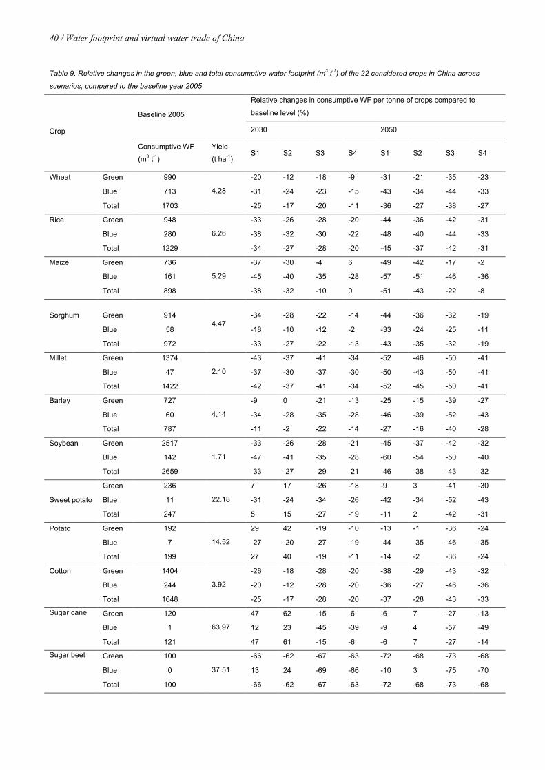
40 / Water footprint and virtual water trade of China
Table 9. Relative changes in the green, blue and total consumptive water footprint (m3 t-1) of the 22 considered crops in China across
scenarios, compared to the baseline year 2005
Crop
Baseline 2005
Relative changes in consumptive WF per tonne of crops compared to
baseline level (%)
2030 2050
Consumptive WF
(m3 t-1)
Yield
(t ha-1) S1 S2 S3 S4 S1 S2 S3 S4
Wheat Green 990
4.28
-20 -12 -18 -9 -31 -21 -35 -23
Blue 713 -31 -24 -23 -15 -43 -34 -44 -33
Total 1703 -25 -17 -20 -11 -36 -27 -38 -27
Rice Green 948
6.26
-33 -26 -28 -20 -44 -36 -42 -31
Blue 280 -38 -32 -30 -22 -48 -40 -44 -33
Total 1229 -34 -27 -28 -20 -45 -37 -42 -31
Maize Green 736
5.29
-37 -30 -4 6 -49 -42 -17 -2
Blue 161 -45 -40 -35 -28 -57 -51 -46 -36
Total 898 -38 -32 -10 0 -51 -43 -22 -8
Sorghum Green 914 4.47
-34 -28 -22 -14 -44 -36 -32 -19
Blue 58 -18 -10 -12 -2 -33 -24 -25 -11
Total 972 -33 -27 -22 -13 -43 -35 -32 -19
Millet Green 1374
2.10
-43 -37 -41 -34 -52 -46 -50 -41
Blue 47 -37 -30 -37 -30 -50 -43 -50 -41
Total 1422 -42 -37 -41 -34 -52 -45 -50 -41
Barley Green 727
4.14
-9 0 -21 -13 -25 -15 -39 -27
Blue 60 -34 -28 -35 -28 -46 -39 -52 -43
Total 787 -11 -2 -22 -14 -27 -16 -40 -28
Soybean Green 2517
1.71
-33 -26 -28 -21 -45 -37 -42 -32
Blue 142 -47 -41 -35 -28 -60 -54 -50 -40
Total 2659 -33 -27 -29 -21 -46 -38 -43 -32
Sweet potato
Green 236
22.18
7 17 -26 -18 -9 3 -41 -30
Blue 11 -31 -24 -34 -26 -42 -34 -52 -43
Total 247 5 15 -27 -19 -11 2 -42 -31
Potato Green 192
14.52
29 42 -19 -10 -13 -1 -36 -24
Blue 7 -27 -20 -27 -19 -44 -35 -46 -35
Total 199 27 40 -19 -11 -14 -2 -36 -24
Cotton Green 1404
3.92
-26 -18 -28 -20 -38 -29 -43 -32
Blue 244 -20 -12 -28 -20 -36 -27 -46 -36
Total 1648 -25 -17 -28 -20 -37 -28 -43 -33
Sugar cane Green 120
63.97
47 62 -15 -6 -6 7 -27 -13
Blue 1 12 23 -45 -39 -9 4 -57 -49
Total 121 47 61 -15 -6 -6 7 -27 -14
Sugar beet Green 100
37.51
-66 -62 -67 -63 -72 -68 -73 -68
Blue 0 13 24 -69 -66 -10 3 -75 -70
Total 100 -66 -62 -67 -63 -72 -68 -73 -68
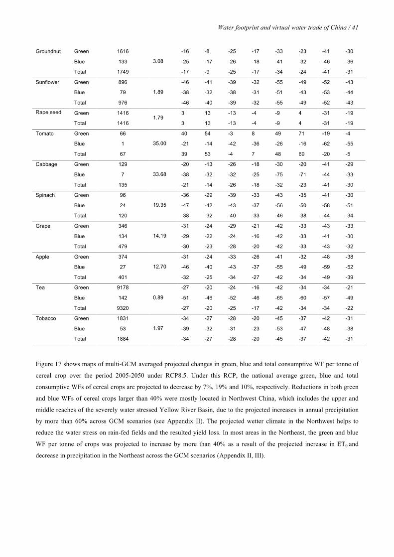
Water footprint and virtual water trade of China / 41
Groundnut Green 1616
3.08
-16 -8 -25 -17 -33 -23 -41 -30
Blue 133 -25 -17 -26 -18 -41 -32 -46 -36
Total 1749 -17 -9 -25 -17 -34 -24 -41 -31
Sunflower Green 896
1.89
-46 -41 -39 -32 -55 -49 -52 -43
Blue 79 -38 -32 -38 -31 -51 -43 -53 -44
Total 976 -46 -40 -39 -32 -55 -49 -52 -43
Rape seed Green 1416 1.79
3 13 -13 -4 -9 4 -31 -19
Total 1416 3 13 -13 -4 -9 4 -31 -19
Tomato Green 66
35.00
40 54 -3 8 49 71 -19 -4
Blue 1 -21 -14 -42 -36 -26 -16 -62 -55
Total 67 39 53 -4 7 48 69 -20 -5
Cabbage Green 129
33.68
-20 -13 -26 -18 -30 -20 -41 -29
Blue 7 -38 -32 -32 -25 -75 -71 -44 -33
Total 135 -21 -14 -26 -18 -32 -23 -41 -30
Spinach Green 96
19.35
-36 -29 -39 -33 -43 -35 -41 -30
Blue 24 -47 -42 -43 -37 -56 -50 -58 -51
Total 120 -38 -32 -40 -33 -46 -38 -44 -34
Grape Green 346
14.19
-31 -24 -29 -21 -42 -33 -43 -33
Blue 134 -29 -22 -24 -16 -42 -33 -41 -30
Total 479 -30 -23 -28 -20 -42 -33 -43 -32
Apple Green 374
12.70
-31 -24 -33 -26 -41 -32 -48 -38
Blue 27 -46 -40 -43 -37 -55 -49 -59 -52
Total 401 -32 -25 -34 -27 -42 -34 -49 -39
Tea Green 9178
0.89
-27 -20 -24 -16 -42 -34 -34 -21
Blue 142 -51 -46 -52 -46 -65 -60 -57 -49
Total 9320 -27 -20 -25 -17 -42 -34 -34 -22
Tobacco Green 1831
1.97
-34 -27 -28 -20 -45 -37 -42 -31
Blue 53 -39 -32 -31 -23 -53 -47 -48 -38
Total 1884 -34 -27 -28 -20 -45 -37 -42 -31
Figure 17 shows maps of multi-GCM averaged projected changes in green, blue and total consumptive WF per tonne of
cereal crop over the period 2005-2050 under RCP8.5. Under this RCP, the national average green, blue and total
consumptive WFs of cereal crops are projected to decrease by 7%, 19% and 10%, respectively. Reductions in both green
and blue WFs of cereal crops larger than 40% were mostly located in Northwest China, which includes the upper and
middle reaches of the severely water stressed Yellow River Basin, due to the projected increases in annual precipitation
by more than 60% across GCM scenarios (see Appendix II). The projected wetter climate in the Northwest helps to
reduce the water stress on rain-fed fields and the resulted yield loss. In most areas in the Northeast, the green and blue
WF per tonne of crops was projected to increase by more than 40% as a result of the projected increase in ET0 and
decrease in precipitation in the Northeast across the GCM scenarios (Appendix II, III).

42 / Water footprint and virtual water trade of China
Figure 17. Changes in green, blue and overall consumptive water footprint (WF) per tonne of cereal crop in China over the
period 2005-2050 under RCP8.5.

Water footprint and virtual water trade of China / 43
In Fig.18 we plotted the relative changes in WF per tonne of the crops studied against the corresponding relative changes
in crop yield under each scenario. The referential line indicates the relative changes in WFs when only yields change
(thus without the effect of changing ET on WFs). The vertical deviation of the dots from the line shows the impact of
changing ET on WFs. The dots below the line, which is the majority, show the positive impact of reduced ET on
reducing the WF per unit mass of crops.
Figure 18. Relationship between relative changes in crop yields and relative changes in corresponding water footprint per
tonne of crop. One dot refers to the projection for one crop under one GCM for one scenario for one year.
Over the period 2005-2050, the total national consumptive WF (in m3 y-1) of crop production increases by 18% under
RCP2.6 (S1 and S2), and by 0.8% under RCP8.5 (S3 and S4), as a result of the combined effect of climate change and
projected changes in harvested crop area. The impact of projected changes in harvested crop area under each RCP (19%
increase from 2005 to 2050 under RCP2.6 and 4% decrease under RCP8.5) on the total WF was significant, because
average ET per hectare over croplands increases by only 3.1% from 2005 to 2050 for RCP2.6 and by 5.6% for RCP8.5.
The total green WF of crop production increases under both RCPs (by 21% from 2005 to 2050 under RCP2.6 and by 4%
under RCP8.5). The total blue WF increases under RCP2.6 (by 4.3% to 2050) and decreases under RCP8.5 (by 10% to
2050).
3.2. Water footprint of food consumption
The water footprint of food consumption per capita in China decreases across all scenarios as compared to the baseline
year (927 m3 cap-1 y-1), driven by the decreased WF per tonne of most crops. The largest decrease in the WF of food
consumption per capita (by 44% to 2050) is observed under scenario S1 (Fig. 19). This large decrease is due to the less-
meat diet combined with the largest decrease in consumptive WF per unit of crops and animal products. S4 shows the
most modest decrease in the WF of food consumption per capita (20% to 2050), which is due to diet type (current-trend
diet) and a relatively low reduction level in the WFs per unit of crop and animal product compared to the other scenarios.
In “current trend” diet scenarios (S2-S4), animal product consumption was the largest contributor (~41-46%) to WF of
food consumption followed by cereal consumption (~31-32%) and oil crop consumption (~14-18%). In the “less meat”
scenario (S1), the WF of animal product consumption decreased significantly (by 65% from 2005 to 2050) and became

44 / Water footprint and virtual water trade of China
the second largest contributor, after cereal consumption, to total WF of Chinese food consumption. This reduction was
driven by decreases in both animal product consumption (by 37% to 2050) and WF per unit calorie of animal products
(by 43% to 2050).
Figure 19. Water footprint of food consumption per capita under the four scenarios of China.
The total national consumptive WF of food consumption is projected to decrease across all scenarios, compared to the
baseline level of 2005 (1212 billion m3 y-1) (Fig. 20). Even under an increased population by 2030, we observe a decrease
in the total WF of consumption. The main reason for this decrease is the decrease in WF per unit of consumed crop and
animal products, and the fact that the population increase to 2030 remains modest. The more significant decrease by 2050
is a combination of the projected declining population and the further decrease in WFs per unit of crops and animal
products. In S1, with the smallest population size and the largest decrease in WF per capita, the total WF of food
consumption drops most, decreasing on average by 24% and 47% by 2030 and 2050, respectively. With the current-trend
diet, the smaller decrease in the WF of food consumption in S4 compared to S2 and S3 results from the relatively large
size of the population and the relatively high WFs per unit of crops and animal products.
Figure 20. Changes in China’s green, blue and total consumptive water footprint of food consumption across scenarios, as
compared to the baseline year 2005. The green, blue and overall consumptive water footprints in 2005 are 1030, 183, and
1212 billion m3 y-1, respectively.
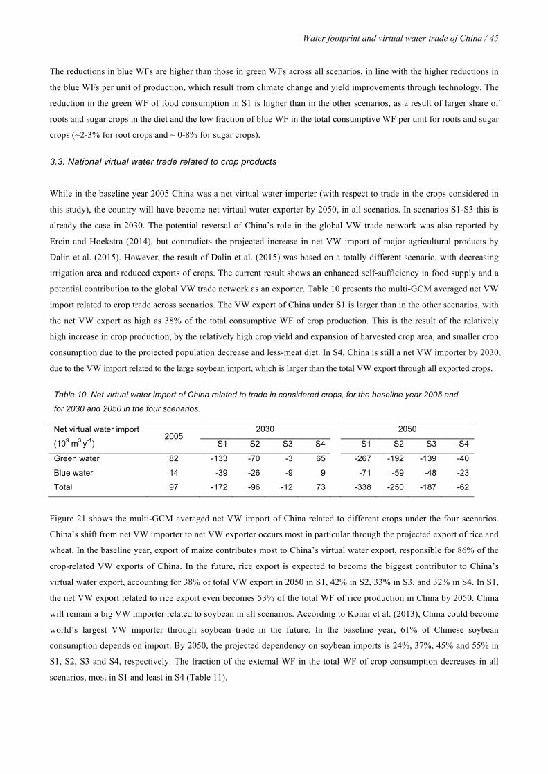
Water footprint and virtual water trade of China / 45
The reductions in blue WFs are higher than those in green WFs across all scenarios, in line with the higher reductions in
the blue WFs per unit of production, which result from climate change and yield improvements through technology. The
reduction in the green WF of food consumption in S1 is higher than in the other scenarios, as a result of larger share of
roots and sugar crops in the diet and the low fraction of blue WF in the total consumptive WF per unit for roots and sugar
crops (~2-3% for root crops and ~ 0-8% for sugar crops).
3.3. National virtual water trade related to crop products
While in the baseline year 2005 China was a net virtual water importer (with respect to trade in the crops considered in
this study), the country will have become net virtual water exporter by 2050, in all scenarios. In scenarios S1-S3 this is
already the case in 2030. The potential reversal of China’s role in the global VW trade network was also reported by
Ercin and Hoekstra (2014), but contradicts the projected increase in net VW import of major agricultural products by
Dalin et al. (2015). However, the result of Dalin et al. (2015) was based on a totally different scenario, with decreasing
irrigation area and reduced exports of crops. The current result shows an enhanced self-sufficiency in food supply and a
potential contribution to the global VW trade network as an exporter. Table 10 presents the multi-GCM averaged net VW
import related to crop trade across scenarios. The VW export of China under S1 is larger than in the other scenarios, with
the net VW export as high as 38% of the total consumptive WF of crop production. This is the result of the relatively
high increase in crop production, by the relatively high crop yield and expansion of harvested crop area, and smaller crop
consumption due to the projected population decrease and less-meat diet. In S4, China is still a net VW importer by 2030,
due to the VW import related to the large soybean import, which is larger than the total VW export through all exported crops.
Table 10. Net virtual water import of China related to trade in considered crops, for the baseline year 2005 and
for 2030 and 2050 in the four scenarios.
Net virtual water import
(109 m3 y-1) 2005
2030
2050
S1 S2 S3 S4
S1 S2 S3 S4
Green water 82 -133 -70 -3 65
-267 -192 -139 -40
Blue water 14 -39 -26 -9 9
-71 -59 -48 -23
Total 97 -172 -96 -12 73 -338 -250 -187 -62
Figure 21 shows the multi-GCM averaged net VW import of China related to different crops under the four scenarios.
China’s shift from net VW importer to net VW exporter occurs most in particular through the projected export of rice and
wheat. In the baseline year, export of maize contributes most to China’s virtual water export, responsible for 86% of the
crop-related VW exports of China. In the future, rice export is expected to become the biggest contributor to China’s
virtual water export, accounting for 38% of total VW export in 2050 in S1, 42% in S2, 33% in S3, and 32% in S4. In S1,
the net VW export related to rice export even becomes 53% of the total WF of rice production in China by 2050. China
will remain a big VW importer related to soybean in all scenarios. According to Konar et al. (2013), China could become
world’s largest VW importer through soybean trade in the future. In the baseline year, 61% of Chinese soybean
consumption depends on import. By 2050, the projected dependency on soybean imports is 24%, 37%, 45% and 55% in
S1, S2, S3 and S4, respectively. The fraction of the external WF in the total WF of crop consumption decreases in all
scenarios, most in S1 and least in S4 (Table 11).

46 / Water footprint and virtual water trade of China
Figure 21. Net virtual water import of China related to its trade in different crops, for the baseline year 2005 and for 2030
and 2050 in the four scenarios.
Table 11. Fraction of the external water footprint (WF) in the total water footprint of Chinese crop consumption, in the
baseline year and in 2030 and 2050 under the four scenarios.
Fraction of external WF in total
WF of crop consumption 2005
2030
2050
S1 S2 S3 S4
S1 S2 S3 S4
Green WF 17% 10% 12% 15% 17%
5% 8% 10% 14%
Blue WF 11% 6% 7% 8% 11%
1% 2% 1% 6%
Consumptive WF 15% 9% 11% 13% 16%
5% 7% 9% 13%
3.4. Discussion
In Table 12 we compare the current results with the results from earlier studies where possible. The relative changes in
WF per tonne of wheat and maize in China in the current study are in the same direction but much larger than the global
average values as suggested by (Fader et al., 2010). The differences in magnitude originate from the different geographic
scopes of the studies, but also from the fact that different climate scenarios and crop models are used. The relative
changes in total blue WF at the current irrigated cropland in China from the current study, which considers the impacts of
both changing precipitation and ET0, are smaller than the estimates for Asia provided by Pfister et al. (2011), who
considers the impact of changing precipitation only. The changes in WF of crop production in China found in the current
study are much smaller than the figures presented by Ercin and Hoekstra (2014). The decrease in total WF of food
consumption in scenario S1 in the current study is greater than the decrease in scenarios S3 and S4 in Ercin and Hoekstra
(2014), which are based on the same less-meat diet scenario, but exclude the effect of reduced WFs per unit of food
products by climate change that has been included in the current study. The relative changes in VW import related to
soybean for S3 in the current study agree best with the result for the low-yield scenario in Konar et al. (2013).

Water footprint and virtual water trade of China / 47
Table 12. Comparison between the current results and previous studies.
Reference Year Study case Scenario Changes in consumptive WF per tonne of
consumed crops (%)
Fader et al. (2010) 2041-70 global wheat
SRES A2 -0.43/-0.45
global maize -0.35/-0.44
Current study
2005-
2050 China wheat RCP 2.6 -27/-36
RCP 8.5 -26/-39
China maize RCP 2.6 -44/-50
RCP 8.5 -7/-23
Year Study case Scenario
Changes in total blue WF at current irrigated area
(%)
Pfister et al.(2011) 2000-
2050 Asia SRES A1B -11
Current study 2005-
2050 China RCP 2.6 -8
RCP 8.5 -2
Year Study case Scenario
Changes in total consumptive WF for crop
production (%)
Ercin and Hoekstra
(2014
2000-
2050 China
"S1/S2/S3/S4"
based on
IPCC AR4
89/127/-22/-22
Current study 2005-
2050
"S1/S2/S3/S4"
based on
IPCC AR5
17/17/0.8/0.8
Year Study case Scenario
Changes in total consumptive WF for crop
consumption (%)
Ercin and Hoekstra
(2014
2000-
2050 China
"S1/S2/S3/S4"
based on
IPCC AR4
79/117/-29/-25
Current study 2005-
2050
"S1/S2/S3/S4"
based on
IPCC AR5
-47/-30/-33/-20
Year Study case Scenario Net virtual water import (109 m3 y-1)
Konar et al. (2013) 2030 Soybean
low yield' /
'high yield'
(SRES A2)
25.44 / 32.44
Ercin and Hoekstra
(2014 2050
Agricultural
products
"S1/S2/S3/S4"
based on
IPCC AR4
-171/-152/ -101/-63
Current study 2030 Soybean "S1/S2/S3/S4"
based on
IPCC AR5
60(-19%)/71(-3%)/ 81(11%)/90(21%)
2050 Crop products -338/-250/-187/-62

48 / Water footprint and virtual water trade of China
Currently, four billion people live under severe blue water scarcity for at least for one month a year, and 0.9 billion of the
four billion live in China (Mekonnen and Hoekstra, 2016). We added the current results on relative changes in national
blue WF (m3 y-1) of crop production in China under each scenario to the context of current China’s total water blue WF
and compare to the current maximum sustainable blue WF (Mekonnen and Hoekstra, 2016). In scenarios S1and S2 under
RCP2.6, the increase of 5% in total blue WF from 2005 to 2050 of crop production will slightly increase current blue
water scarcity of China as a whole from 0.49 (low blue water scarcity) (Mekonnen and Hoekstra, 2016) to 0.51
(moderate blue water scarcity). The projected decrease of 9% in total blue WF of China’s crop production in S3 and S4
under RCP8.5 will reduce the current blue water scarcity accordingly to 0.45. There have been studies on changes in blue
water availability in China to future climate changes (Hanasaki et al., 2013b; Elliott et al., 2014; Santini and di Paola,
2015). The finding on significant decrease in blue water availability in the Yellow River Basin of more than 40% from
2005 to 2050 under RCP 8.5 was unified across these studies. According to the current study, even though the total blue
WF of crop production in the Yellow River Basin will decrease by 11% under RCP 8.5 (S3 and S4), the basin could still
suffer increasing blue water scarcity from the possible declining runoff. While for other parts of China, the current level
of blue water scarcity (Mekonnen and Hoekstra, 2016) will not change significantly for considered scenarios from 2005
to 2050, given the projected slight increase (~10%) in blue water availability (Hanasaki et al., 2013b; Elliott et al., 2014;
Santini and di Paola, 2015) and current projected slight increase (~4%) in total blue WF of crop production under
RCP2.6 and decreases (~10%) under RCP8.5.
In addition, there are inherent uncertainties in scenario studies. All scenarios are based on assumptions regarding climate
change and socio-economic developments like population growth, changes in diets, technological improvements and land
use changes. Different GCMs result in different climate projections for a given emission scenario, which can be
addressed by using the projections from multiple GCMs (Semenov and Stratonovitch, 2010), as we did in the current
study, although we considered four GCMs only. Finally, the crop model used, the Aquacrop model in our study, and
parameter values chosen, will inevitably result in different yield predictions when compared to studies based other
models and parameter sets (Asseng et al., 2013).

4. Conclusion
The study provides a comprehensive analysis of the consumptive WF and VW trade of China by 2030 and 2050,
focusing on the agricultural sector, developing four alternative scenarios forced by different levels of population growth
and by changes in production, consumption and climate. The four scenarios differ in assumptions and outcomes, but the
projected futures share a few commonalities:
(i) On average, the WF of producing a tonne of crop decreases due to the combined effect of climate change
and technology improvements on yield increase. Wetter climate projections in Northwest China potentially
reduce the local blue WF of crop production that can help to reduce the high blue water stress from the
agriculture sector;
(ii) The WF of food consumption per capita decreases, up to 44% by 2050 if diets change to less meat (scenario
S1). The total national WF of food consumption also decreases across all scenarios;
(iii) China will shift from net VW importer through crop trade to net VW exporter. However, China will remain
depending on soybean imports.
The results suggest that the target of the Chinese government to achieve higher self-sufficiency in food supply while
simultaneously reducing the WF of crop production (SCPRC, 2010; MOA et al., 2015) is feasible. However, the premise
of realizing the presented scenarios is smart water and cropland management, effective and coherent policies on water,
agriculture and infrastructure, and, in scenario S1, a successful shift to a diet containing less meat.


References
Allen, R.G., Pereira, L.S., Raes, D. and Smith, M. (1998) Crop evapotranspiration-Guidelines for computing
crop water requirements-FAO Irrigation and drainage paper 56. FAO, Rome 300(9): D05109.
Asseng, S., Ewert, F., Rosenzweig, C., Jones, J.W., Hatfield, J.L., Ruane, A.C., Boote, K.J., Thorburn, P.J.,
Rotter, R.P., Cammarano, D., Brisson, N., Basso, B., Martre, P., Aggarwal, P.K., Angulo, C., Bertuzzi,
P., Biernath, C., Challinor, A.J., Doltra, J., Gayler, S., Goldberg, R., Grant, R., Heng, L., Hooker, J.,
Hunt, L.A., Ingwersen, J., Izaurralde, R.C., Kersebaum, K.C., Muller, C., Naresh Kumar, S., Nendel,
C., O/'Leary, G., Olesen, J.E., Osborne, T.M., Palosuo, T., Priesack, E., Ripoche, D., Semenov, M.A.,
Shcherbak, I., Steduto, P., Stockle, C., Stratonovitch, P., Streck, T., Supit, I., Tao, F., Travasso, M.,
Waha, K., Wallach, D., White, J.W., Williams, J.R. and Wolf, J. (2013) Uncertainty in simulating
wheat yields under climate change. Nature Climate Change 3(9): 827-832.
Barnett, J., Rogers, S., Webber, M., Finlayson, B. and Wang, M. (2015) Sustainability: Transfer project cannot
meet China's water needs, Nature 527(7578): 295-297.
Batjes, N.H. (2012) ISRIC-WISE global data set of derived soil properties on a 5 by 5 arc-minutes grid (version
1.2). Report 2012/01, ISRIC World Soil Information, Wageningen, the Netherlands.
Barriopedro, D., Gouveia, C.M., Trigo, R.M. and Wang, L. (2012) The 2009/10 drought in China: possible
causes and impacts on vegetation. Journal of Hydrometeorology 13: 1251-1267.
Bouwman, A., Van der Hoek, K., Eickhout, B. and Soenario, I. (2005) Exploring changes in world ruminant
production systems. Agricultural Systems 84(2): 121-153.
Bruinsma, J. (2003) World agriculture: towards 2015/2030: an FAO perspective, Earthscan, London, UK.
Cao, X., Wu, P., Wang, Y., Zhao, X. and Li, S. (2011) Application of virtual water trade theory in inter-regional
grain allocation and transportation in China. African Journal of Biotechnology 10(80): 18463–18471.
Cao, X., Wu, P., Wang, Y. and Zhao, X. (2015) Challenge of water sources in urbanizing China: an analysis of
agricultural water footprint. Polish Journal of Environmental Studies 24 (1): 9-18.
Cao, X. C., Wu, P.T., Wang, Y. B. and Zhao, X.N. (2014a) Water footprint of grain product in irrigated
farmland of China. Water Resources Management 28 (8): 2213-2227.
Cao, X.C., Wu, P.T., Wang, Y.B. and Zhao, X.N. (2014b) Assessing blue and green water utilisation in wheat
production of China from the perspectives of water footprint and total water use. Hydrology and Earth
System Sciences 18: 3165-3178.
Chapagain, A.K., Hoekstra, A.Y. and Savenije, H.H.G. (2006) Water saving through international trade of
agricultural products. Hydrology and Earth System Sciences 10: 455-468.
Chen, Z. M. and Chen, G.Q. (2013) Virtual water accounting for the globalized world economy: national water
footprint and international virtual water trade. Ecological Indicators 28: 142-149.
Chilonda, P. and Otte, J. (2006) Indicators to monitor trends in livestock production at national, regional and
international levels. Livestock Research for Rural Development 18 (8):117.
Chukalla, A.D., Krol , M.S. and Hoekstra, A.Y. (2015) Green and blue water footprint reduction in irrigated
agriculture: Effect of irrigation techniques, irrigation strategies and mulching. Hydrology and Earth
System Sciences 19 (12): 4877–4891.

52 / Water footprint and virtual water trade of China
Dalin, C., Konar, M., Hanasaki, N., Rinaldo, A. and Rodriguez-Iturbe, I. (2012) Evolution of the global virtual
water trade network. Proceedings of the National Academy of Sciences of the United States of America
109(16): 5989-5994.
Dalin, C., Hanasaki, N., Qiu, H., Mauzerall, D. L. and Rodriguez-Iturbe, I. (2014) Water resources transfer
through Chinese interprovincial and foreign food trade. Proceedings of the National Academy of
Sciences of the United States of America 111(27): 9774–9779.
Dalin, C., Qiu, H., Hanasaki, N., Mauzerall, D.L. and Rodriguez-Iturbe, I. (2015) Balancing water resource
conservation and food security in China. Proceedings of the National Academy of Sciences of the
United States of America 112(15): 4588-4593.
De Fraiture, C., Wichelns, D., Rockstrom, J., Kemp-Benedict, E., Eriyagama, N., Gordon, L.J., Hanjra, M.A.,
Hoogeveen, J., Huber-Lee, A. and Karlberg, L. (2007) Water for food, water for life: a Comprehensive
Assessment of Water Management in Agriculture. Molden, D. (ed), pp. 91-145, Earthscan, London,
UK; International Water Management Institute, Colombo, Sri Lanka.
Dijkshoorn, J.A., van Engelen, V.W.P. and Huting, J.R.M. (2008) Soil and landform properties for LADA
partner countries (Argentina, China, Cuba, Senegal and The Gambia, South Africa and Tunisia). ISRIC
report 2008/06, ISRIC World Soil Information, Wageningen, the Netherlands.
Dobor, L., Barcza, Z., Hlásny, T., Árendás, T., Spitkó, T. and Fodor, N. (2016) Crop planting date matters:
estimating methods and effect on future yields. Agricultural and Forest Meteorology 223: 103-115.
Du, S.F., Mroz, T.A., Zhai, F. and Popkin, B.M. (2004) Rapid income growth adversely affects diet quality in
China—particularly for the poor! Social Science & Medicine 59 (7): 1505-1515.
Elliott, J., Deryng, D., Müller, C., Frieler, K., Konzmann, M., Gerten, D., Glotter, M., Flörke, M., Wada, Y.,
Best, N., Eisner, S., Fekete, B. M., Folberth, C., Foster, I., Gosling, S. N., Haddeland, I., Khabarov, N.,
Ludwig, F., Masaki, Y., Olin, S., Rosenzweig, C., Ruane, A. C., Satoh, Y., Schmid, E., Stacke, T.,
Tang, Q. and Wisser, D. (2014) Constraints and potentials of future irrigation water availability on
agricultural production under climate change. Proceedings of the National Academy of Sciences of the
United States of America 111 (9): 3239-3244.
Erb, K.-H., Haberl, H., Krausmann, F., Lauk, C., Plutzar, C., Steinberger, J.K., Müller, C., Bondeau, A., Waha,
K. and Pollack, G. (2009) Eating the Planet: Feeding and fuelling the world sustainably, fairly and
humanely - a scoping study. Commissioned by Compassion in World Farming and Friends of the Earch
UK. Institute of Social Ecology and PIK Potsdam, Vienna, Potsdam.
Ercin, A.E. and Hoekstra, A.Y. (2014) Water footprint scenarios for 2050: A global analysis. Environment
International 64: 71-82.
Fader, M., Rost, S., Müller, C., Bondeau, A. and Gerten, D. (2010) Virtual water content of temperate cereals
and maize: Present and potential future patterns. Journal of Hydrology 384: 218–231.
Fader, M., Gerten, D., Thammer, M., Heinke, J., Lotze-Campen, H., Lucht, W. and Cramer, W. (2011) Internal
and external green-blue agricultural water footprints of nations, and related water and land savings
through trade, Hydrology and Earth System Sciences 15(5): 1641-1660.
Falkenmark, M. (2013) Growing water scarcity in agriculture: future challenge to global water security.
Philosophical Transactions of the Royal Society a-Mathematical Physical and Engineering Sciences
371(2002): 20120410.

Water footprint and virtual water trade of China / 53
Falkenmark, M. and Rockström, J. (2004) Balancing water for humans and nature: The new approach in
ecohydrology, Earthscan, London, UK.
Fang, D.L. and Chen, B. (2015) Ecological network analysis for a virtual water network. Environmental Science
& Technology 49: 6722-6730.
FAO (2005) Livestock, Environment and Development Initiative 2005. Food and Agricultural Organization,
Rome, Italy.
FAO(2014) FAOSTAT, Food and Agriculture Organization, Rome, Italy. http://faostat.fao.org.
Feng, K., Hubacek, K., Pfister, S., Yu, Y. and Sun, L. (2014) Virtual scarce water in China. Environmental
Science & Technology 48: 7704-7713.
Ge, L., Xie, G., Zhang, C., Li, S., Qi, Y., Cao, S. and He, T. ( 2011) An evaluation of China’s water footprint.
Water Resources Management 25: 2633-2647.
Gong, P., Yin, Y. and Yu, C. (2011) China: invest wisely in sustainable water use. Science 331: 1264.
Guan, D. and Hubacek, K. (2007) Assessment of regional trade and virtual water flows in China. Ecological
Economics 61: 159-170.
Haddeland, I., Heinke, J., Biemans, H., Eisner, S., Flörke, M., Hanasaki, N., Konzmann, M., Ludwig, F.,
Masaki, Y. and Schewe, J. (2014) Global water resources affected by human interventions and climate
change. Proceedings of the National Academy of Sciences of the United States of America 111(9):
3251-3256.
Hanasaki, N., Fujimori, S., Yamamoto, T., Yoshikawa, S., Masaki, Y., Hijioka, Y., Kainuma, M., Kanamori, Y.,
Masui, T. and Takahashi, K. (2013a) A global water scarcity assessment under Shared Socio-economic
Pathways–Part 1: Water use. Hydrology and Earth System Sciences 17(7): 2375-2391.
Hanasaki, N., Fujimori, S., Yamamoto, T., Yoshikawa, S., Masaki, Y., Hijioka, Y., Kainuma, M., Kanamori, Y.,
Masui, T. and Takahashi, K. (2013b) A global water scarcity assessment under Shared Socio-economic
Pathways–Part 2: Water availability and scarcity. Hydrology and Earth System Sciences 17(7): 2393-
2413.
Han, X. and Sun, C. (2013) Virtual water flow patterns embedded in major crops in China. Resources Science
35(8): 1567-1576 (in Chinese).
Harris, I., Jones, P. D., Osborn, T. J. and Lister, D. H. (2014) Updated high-resolution grids of monthly climatic
observations - the CRU TS3.10 dataset. International Journal of Climatology 34(3): 623–642.
Hatfield, J.L., Boote, K.J., Kimball, B.A., Ziska, L.H., Izaurralde, R.C., Ort, D., Thomson, A.M. and Wolfe, D.
(2011) Climate Impacts on Agriculture: Implications for Crop Production. Agronomy Journal 103(2):
351-370.
Hoekstra, A. Y. (Ed.) (2003) Virtual water trade, in: Proceedings of the International Expert Meeting on Virtual
Water Trade. IHE Delft, the Netherlands, 12–13 December 2002. Value of Water Research Report
Series No. 12, UNESCO-IHE, Delft, the Netherlands.
Hoekstra, A.Y. (2013) The water footprint of modern consumer society. Routledge, London, UK.
Hoekstra, A.Y. and Chapagain, A.K. (2007) Water footprints of nations: water use by people as a function of
their consumption pattern. Water Resources Management 21(1): 35-48.
Hoekstra, A.Y. and Chapagain, A.K. (2008) Globalization of water: Sharing the planet's freshwater resources.
Blackwell, Oxford, UK.

54 / Water footprint and virtual water trade of China
Hoekstra, A. Y., Chapagain, A. K., Aldaya, M. M. and Mekonnen, M. M. (2011) The water footprint assessment
manual: Setting the global standard. Earthscan, London, UK.
Hoekstra, A.Y. and Hung, P.Q. (2005) Globalisation of water resources: international virtual water flows in
relation to crop trade. Global Environmental Change 15(1): 45-56.
Hoekstra, A.Y. and Mekonnen, M.M. (2012) The water footprint of humanity. Proceedings of the National
Academy of Sciences of the United States of America 109(9): 3232−3237.
Hoekstra, A.Y. and Wiedmann, T.O. (2014) Humanity's unsustainable environmental footprint. Science
344(6188): 1114-1117.
Hsiao, T.C., Heng, L., Steduto, P., Rojas-Lara, B., Raes, D. and Fereres, E. (2009) AquaCrop—The FAO crop
model to simulate yield response to water. III. Parameterization and testing for maize, Agronomy
Journal 101(3): 448-459.
Huang, J., Pray, C. and Rozelle, S. (2002) Enhancing the crops to feed the poor. Nature 418(6898): 678-684.
Hurtt, G.C., Chini, L.P., Frolking, S., Betts, R.A., Feddema, J., Fischer, G., Fisk, J.P., Hibbard, K., Houghton,
R.A., Janetos, A., Jones, C.D., Kindermann, G., Kinoshita, T., Goldewijk, K.K., Riahi, K.,
Shevliakova, E., Smith, S., Stehfest, E., Thomson, A., Thornton, P., van Vuuren, D.P. and Wang, Y.P.
(2011) Harmonization of land-use scenarios for the period 1500-2100: 600 years of global gridded
annual land-use transitions, wood harvest, and resulting secondary lands. Climatic Change 109(1-2):
117-161.
IIASA (2009) RCP Database. http://www.iiasa.ac.at/web-apps/tnt/RcpDb.
IIASA (2013) SSP Database. https://secure.iiasa.ac.at/web-apps/ene/SspDb/dsd.
IPCC (2014) Climate Change 2014: Synthesis Report. Contribution of Working Groups I, II and III to the Fifth
Assessment Report of the Intergovernmental Panel on Climate Change. IPCC. Switherlands.
Jiang, Y. (2009) China's water scarcity. Journal of Environmental Management 90(11): 3185-3196.
Jiang, Y. (2015) China's water security: Current status, emerging challenges and future prospects.
Environmental Science & Policy 54: 106-125.
Jiang, Y., Cai, W., Du, P., Pan, W. and Wang, C. (2015) Virtual water in interprovincial trade with implications
for China's water policy. Journal of Cleaner Production 87: 655-665.
Keyzer, M.A., Merbis, M.D., Pavel, I.F.P.W. and van Wesenbeeck, C.F.A. (2005) Diet shifts towards meat and
the effects on cereal use: can we feed the animals in 2030? Ecological Economics 55(2): 187-202.
Konar, M., Hussein, Z., Hanasaki, N., Mauzerall, D.L. and Rodriguez-Iturbe, I. (2013) Virtual water trade flows
and savings under climate change. Hydrology and Earth System Sciences 17(8): 3219-3234.
Kriegler, E., O'Neill, B.C., Hallegatte, S., Kran, T., Lempert, R., Moss, R.H. and Wilbanks, T.J. (2010) Socio-
economic scenario development for climate change analysis. CIRED Working Paper DT/WP No 2010-
23. October 2010.
Liu, J. and Savenije, H. H. G. (2008) Food consumption patterns and their effect on water requirement in China.
Hydrology and Earth System Sciences 12: 887-898.
Liu, J., Yang, H. (2010) Spatially explicit assessment of global consumptive water uses in cropland: green and
blue water. Journal of Hydrology 384: 187–197.
Liu, J., Zehnder, A. J. B. and Yang, H. (2007) Historical trends in China's virtual water trade. Water
International 32(1): 78-90.

Water footprint and virtual water trade of China / 55
Liu, J.G., Folberth, C., Yang, H., Rockstrom, J., Abbaspour, K. and Zehnder, A.J.B. (2013) A Global and
Spatially Explicit Assessment of Climate Change Impacts on Crop Production and Consumptive Water
Use. PLoS One 8(2): e57750.
Lovarelli, D., Bacenetti, J. and Fiala, M. (2016) Water footprint of crop productions: a review. Science of the
Total Environment 548-549: 236-251.
Lu, C.H. and Fan, L. (2013) Winter wheat yield potentials and yield gaps in the North China Plain. Field Crops
Research 143: 98-105.
Lu, E., Luo, Y., Zhang, R., Wu, Q. and Liu, L. (2011) Regional atmospheric anomalies responsible for the
2009–2010 severe drought in China. Journal of Geophysical Research 116: D21114.
Ma, J., Hoekstra, A.Y., Wang, H., Chapagain, A.K. and Wang, D. (2006) Virtual versus real water transfers
within China. Philosophical Transactions of the Royal Society B 361 (1469): 835-842.
Mekonnen, M.M. and Hoekstra, A.Y. (2011) The green, blue and grey water footprint of crops and derived crop
products. Hydrology and Earth System Sciences 15(5):1577-1600.
Mekonnen, M.M. and Hoekstra, A.Y. (2012) A Global Assessment of the Water Footprint of Farm Animal
Products. Ecosystems 15(3): 401-415.
Mekonnen, M.M. and Hoekstra, A.Y. (2016) Four billion people facing severe water scarcity, Science
Advances, 2(2): e1500323.
Meng, Q.F., Hou, P., Wu, L., Chen, X.P., Cui, Z.L. and Zhang, F.S. (2013) Understanding production potentials
and yield gaps in intensive maize production in China. Field Crops Research 143: 91-97.
MOA, NDRC, MOST, MOF, MLR, MEP, MWR and SFA (2015) National Plan of Sustainable Agriculture
(2015-2030), Ministry of Agriculture of P. R. China; National Development and Reform Commission,
P. R. China; Ministry of Science and Technology of P. R. China; Ministry of Finance of P.R.China;
Ministry of Land and Resources of P.R.China; Ministry of Environmental Protection of P.R.China;
Ministry of Water Resources of P.R.China; State Forestry Administration of P.R.China, Beijing, China.
Monfreda, C., Ramankutty, N. and Foley, J. A. (2008) Farming the planet: 2. Geographic distribution of crop
areas, yields, physiological types, and net primary production in the year 2000. Global Biogeochemical
Cycles 22: GB1022.
Moss, R.H., Edmonds, J.A., Hibbard, K.A., Manning, M.R., Rose, S.K., van Vuuren, D.P., Carter, T.R., Emori,
S., Kainuma, M., Kram, T., Meehl, G.A., Mitchell, J.F.B., Nakicenovic, N., Riahi, K., Smith, S.J.,
Stouffer, R.J., Thomson, A.M., Weyant, J.P. and Wilbanks, T.J. (2010) The next generation of
scenarios for climate change research and assessment. Nature 463(7282): 747-756.
Mu, J.X. and Khan, S. (2009) The effect of climate change on the water and food nexus in China. Food Security
1(4): 413-430.
Mueller, N.D., Gerber, J.S., Johnston, M., Ray, D.K., Ramankutty, N. and Foley, J.A. (2012) Closing yield gaps
through nutrient and water management. Nature 490(7419): 254-257.
MWR (2015) Water resources bulletin of China 2014, Ministry of Water Resources, P.R. China, Beijing, China.
MWR (2014) Water resources bulletin of China 2013. Ministry of Water Resources, Beijing, China.
NASMG (2010) Surveying and mapping data sharing network. National Administration of Surveying, Mapping
and Geo-information, China.
NBSC (2013) National data. National Bureau of Statistics of China. Beijing, China.

56 / Water footprint and virtual water trade of China
NDRC (2007) China's national climate change programme, National Development and Reform Commission, P.
R. China, Beijing, China.
NDRC (2008) Long-term plan for national grain security (2008-2020), National Development and Reform
Commission, P. R. China, Beijing, China.
Nonhebel, S. and Kastner, T. (2011) Changing demand for food, livestock feed and biofuels in the past and in
the near future. Livestock Science 139(1): 3-10.
O’Neill, B., Carter, T., Ebi, K., Edmonds, J., Hallegatte, S., Kemp-Benedict, E., Kriegler, E., Mearns, L., Moss,
R. and Riahi, K. (2012) Meeting Report of the workshop on the nature and use of new socioeconomic
pathways for climate change research, Boulder, CO, November 2–4, 2011,Workshop report, Boulder:
National Center for Atmospheric Research,
Pfister, S., Bayer, P., Koehler, A. and Hellweg, S. (2011) Projected water consumption in future global
agriculture: scenarios and related impacts. Science of the Total Environment 409(20): 4206-4216.
Piao, S., Ciais, P., Huang, Y., Shen, Z., Peng, S., Li, J., Zhou, L., Liu, H., Ma, Y. and Ding, Y. (2010) The
impacts of climate change on water resources and agriculture in China. Nature 467(7311): 43-51.
Polasky, S., Carpenter, S.R., Folke, C. and Keeler, B. (2011) Decision-making under great uncertainty:
environmental management in an era of global change. Trends in Ecology & Evolution 26(8): 398-404.
Portmann, F.T., Siebert, S. and Döll, P. (2010) MIRCA2000 – Global monthly irrigated and rain-fed crop areas
around the year 2000: A new high-resolution data set for agricultural and hydrological modelling.
Global Biogeochemical Cycles 24: GB1011.
Raes, D., Steduto, P., Hsiao, T.C. and Fereres, E. (2009) AquaCrop – The FAO crop model to simulate yield
response to water. II. Main algorithms and software description. Agronomy Journal 101(3): 438-477.
Ramirez-Villegas, J. and Jarvis, A. (2010) Downscaling global circulation model outputs: the delta method
decision and policy analysis Working Paper No. 1. Policy Analysis 1: 1-18.
Rao, S. and Riahi, K. (2006) The role of Non-CO2 greenhouse gases in climate change mitigation: Long-term
scenarios for the 21st century. Energy Journal: 177-200.
Riahi, K., Grubler, A. and Nakicenovic, N. (2007) Scenarios of long-term socio-economic and environmental
development under climate stabilization. Technological Forecasting and Social Change 74(7): 887-935.
Rosegrant, M.W., Leach, N. and Gerpacio, R.V. (1999) Alternative futures for world cereal and meat
consumption. Proceedings of the Nutrition Society 58(2): 219-234.
Santini, M. and di Paola, A. (2015) Changes in the world rivers’ discharge projected from an updated high
resolution dataset of current and future climate zones. Journal of Hydrology 531 (3): 768-780.
SCPRC (2010) No.1 Document of 2011. State Council of the P.R. China, Beijing, China.
SCPRC (2014) Middle Route Project (MRP), Office of the South-to-North Water Diversion Project Commission,
State Council of the P.R. China, Beijing, China.
Semenov, M.A. and Stratonovitch, P. (2010) Use of multi-model ensembles from global climate models for
assessment of climate change impacts. Climate Research 41(1): 1-14.
Shi, J., Liu, J. and Pinter, L. (2014) Recent evolution of China’s virtual water trade: analysis of selected crops
and considerations for policy. Hydrology and Earth System Science 18: 1349-1357.Shiferaw, B.,
Prasanna, B.M., Hellin, J. and Banziger, M. (2011) Crops that feed the world 6. Past successes and
future challenges to the role played by maize in global food security. Food Security 3(3): 307-327.

Water footprint and virtual water trade of China / 57
SIC (State Information Center) (2005) Multi-regional input-output model for China (1997). Social Sciences
Academic Press, Beijing, China (in Chinese).
Siebert, S. and Döll, P. (2010) Quantifying blue and green virtual water contents in global crop production as
well as potential production losses without irrigation. Journal of Hydrology 384: 198–217.
Steduto, P., Hsiao, T.C., Raes, D. and Fereres, E. (2009) AquaCrop - the FAO crop model to simulate yield
response to water. I. Concepts and underlying principles. Agronomy Journal 101(3): 426–437.
Sun, S., Wu, P., Wang, Y., Zhao, X., Liu, J. and Zhang, X. (2012) The temporal and spatial variability of water
footprint of grain: A case study of an irrigation district in China from 1960 to 2008. Journal of Food,
Agriculture & Environment 10: 1246-1251.
Sun, S.K., Wu, P. T., Wang, Y.B. and Zhao, X. N. (2013) The virtual water content of major grain crops and
virtual water flows between regions in China. Journal of the Science of Food and Agriculture 93(6):
1427-1437.
Tao, F.L. and Zhang, Z. (2011) Impacts of climate change as a function of global mean temperature: maize
productivity and water use in China. Climatic Change 105(3-4): 409-432.
Taylor, K.E., Stouffer, R.J.,Meehl, G.A., 2012. An overview of CMIP5 and the experiment design. Bulletin of
the American Meteorological Society 93(4): 485–498.
Thomas, A. (2008) Agricultural irrigation demand under present and future climate scenarios in China. Global
and Planetary Change 60(3-4): 306-326.
Tian, Y. H., Zhu, D. J., Wang, H. M. and Zang, M. D. (2013) Water footprint calculation of China’s main food
crops: 1978 – 2010. China Population Resources and Environment 154(06): 124-130 (in Chinese).
Trostle, R. (2008) Global Agricultural Supply and Demand: Factors Contributing to the Recent Increase in Food
Commodity Prices. A report from the economic research services. USA.
Tuninetti, M., Tamea, S., D'Odorico, P., Laio, F. and Ridolfi, L. (2015) Global sensitivity of high-resolution
estimates of crop water footprint. Water Resources Research 51(10): 8257-8272.
Vanham, D. (2016) Does the water footprint concept provide relevant information to address the water–food–
energy–ecosystem nexus? Ecosystem Services 17: 298-307.
van Vuuren, D.P., Den Elzen, M.G.J., Lucas, P.L., Eickhout, B., Strengers, B.J., van Ruijven, B., Wonink, S.
and van Houdt, R. (2007) Stabilizing greenhouse gas concentrations at low levels: an assessment of
reduction strategies and costs. Climatic Change 81(2): 119-159.
van Vuuren, D.P., Edmonds, J., Kainuma, M., Riahi, K., Thomson, A., Hibbard, K., Hurtt, G.C., Kram, T.,
Krey, V., Lamarque, J.F., Masui, T., Meinshausen, M., Nakicenovic, N., Smith, S.J. and Rose, S.K.
(2011) The representative concentration pathways: an overview. Climatic Change 109(1-2): 5-31.
Wada, Y. and Bierkens, M.F.P. (2014) Sustainability of global water use: past reconstruction and future
projections. Environmental Research Letters 9(10): 104003.
Wada, Y., Wisser, D., Eisner, S., Florke, M., Gerten, D., Haddeland, I., Hanasaki, N., Masaki, Y., Portmann,
F.T., Stacke, T., Tessler, Z. and Schewe, J. (2013) Multimodel projections and uncertainties of
irrigation water demand under climate change. Geophysical Research Letters 40(17): 4626-4632.
Waha, K., van Bussel, L. G. J., Müller, C. and Bondeau, A. (2012) Climate-driven simulation of global crop
sowing dates. Global Ecology and Biogeography 21: 247–259.

58 / Water footprint and virtual water trade of China
Wang, S. and Feng, J. (2009) Drought situation and its impacts during April to June 2009 in China. Journal of
Arid Meteorology 27(2): 193-196 (in Chinese).
Wang, Y.B., Wu, P. T., Zhao, X. N. and Engel, B.A. (2014) Virtual water flows of grain within China and its
impact on water resource and grain security in 2010. Ecological Engineering 69: 255-264.
Wu, P., Zhao, X., Cao, X. and Hao, S. (2010) Status and thoughts of Chinese “agricultural north-to-south water
diversion virtual engineering”. Transactions of the CSAE 26(6): 1-6 (in Chinese).
Xiong, W., Holman, I., Lin, E.D., Conway, D., Jiang, J.H., Xu, Y.L. and Li, Y. (2010) Climate change, water
availability and future cereal production in China. Agriculture Ecosystems & Environment 135(1-2):
58-69.
Yao, F.M., Xu, Y.L., Lin, E.D., Yokozawa, M. and Zhang, J.H. (2007) Assessing the impacts of climate change
on rice yields in the main rice areas of China. Climatic Change 80(3-4): 395-409.
Yu, C. (2011) China’s water crisis needs more than words. Nature 470: 307.
Zhang, C. and Anadon, L.D. (2014) A multi-regional input–output analysis of domestic virtual water trade and
provincial water footprint in China. Ecological Economics 100: 159-172.
Zhang, L., Xia, J. and Hu, Z. (2009) Situation and problem analysis of water resource security in China.
Resources and Environment in the Yangtze Basin 18 (2): 116-120.
Zhang, T.Y., Yang, X.G., Wang, H.S., Li, Y. and Ye, Q. (2014) Climatic and technological ceilings for Chinese
rice stagnation based on yield gaps and yield trend pattern analysis. Global Change Biology 20(4):
1289-1298.
Zhang, Y. and Qi, S. (2011) China multi-regional input-output models (2002, 2007). China Statistics Press,
Beijing (in Chinese).
Zhang, Z., Yang, H. and Shi, M. (2011) Analyses of water footprint of Beijing in an interregional input-output
framework. Ecological Economics 70: 2494-2502.
Zhao, C.F. and Chen, B. (2014) Driving force analysis of the agricultural water footprint in China based on the
LMDI method. Environmental Science & Technology 48: 12723-12731.
Zhao, Q.B., Liu, J.G., Khabarov, N., Obersteiner, M. and Westphal, M. (2014) Impacts of climate change on
virtual water content of crops in China. Ecological Informatics 19: 26-34.
Zhao, X., Liu, J., Liu, Q., Tillotson, M. R., Guan, D. and Hubacek, K. (2015) Physical and virtual water
transfers for regional water stress alleviation in China. Proceedings of the National Academy of
Sciences 112(4): 1031-1035.
Zhu, X., Li, Y., Li, M., Pan, Y. and Shi, P. (2013) Agricultural irrigation in China. Journal of Soil and Water
Conservation 68(6): 147A-154A.
Zhu, X.F., Zhao, A.Z., Li, Y.Z. and Liu, X.F. (2015) Agricultural irrigation requirements under future climate
scenarios in China. Journal of Arid Land 7(2): 224-237.
Zhuo, L., Mekonnen, M.M. and Hoekstra, A.Y. (2014) Sensitivity and uncertainty in crop water footprint
accounting: a case study for the Yellow River Basin. Hydrology and Earth System Sciences 18: 2219-
2234.
Zhuo, L., Mekonnen, M.M., Hoekstra, A.Y., Wada, Y. (2016a) Inter- and intra-annual variation of water
footprint of crops and blue water scarcity in the Yellow River Basin (1961-2009). Advances in Water
Resources 87:21-41.

Water footprint and virtual water trade of China / 59
Zhuo, L., Mekonnen, M.M. and Hoekstra, A.Y. (2016b) The effect of inter-annual variability of consumption,
production, trade and climate on crop-related green and blue water footprints and inter-regional virtual
water trade: A study for China (1978-2008), Water Research 94: 73–85.
Zhuo, L., Mekonnen, M.M. and Hoekstra, A.Y. (2016c) Consumptive water footprint and virtual water trade
scenarios for China – with a focus on crop production, consumption and trade, Environment
International 94: 211–223.


App
endi
x I.
An
exam
ple
of a
sses
sing
the
wat
er fo
otpr
int r
elat
ed to
cro
p co
nsum
ptio
n in
Chi
na: w
heat
in th
e ye
ar 2
006
A
. Nat
iona
l tot
al c
rop
utili
zatio
n an
d su
pply
acc
ount
s ar
e ob
tain
ed fr
om F
AO
(201
4).
B. S
tatis
tics
on p
rovi
ncia
l pop
ulat
ion
and
lives
tock
are
obt
aine
d fro
m N
BS
C (2
013)
. C
. Pos
itive
val
ue m
eans
impo
rt. N
egat
ive
valu
e m
eans
exp
ort.
D. P
rovi
ncia
l “cr
op tr
ade
bala
nce”
refe
rs to
net
cro
p im
port.
E
. “Fo
od” i
s eq
ual t
o th
e su
m o
f ”fo
od d
irect
ly” a
nd ”f
ood
man
ufac
ture
d” o
btai
ned
from
FA
O (2
014)
.
Food
EFe
edSe
edW
aste
Oth
erus
ePr
oduc
tion
Stoc
k va
r.In
tern
atio
nal
trade
CIn
ter-
regi
onal
trade
Crop
trad
eba
lanc
eDBl
ueG
reen
Tota
lBl
ueG
reen
Tota
lBl
ueG
reen
Tota
lBl
ueG
reen
Tota
lBl
ueG
reen
Tota
lBl
ueG
reen
Tota
lBe
ijing
1601
6111
0915
4931
2830
0-8
1292
894
017
774
251
0.5
2323
533
578
1111
534
601
1134
574
680
1254
681
646
1327
Tian
jin10
7562
745
1533
2119
499
-13
534
234
733
516
550
00.
28
919
721
341
019
722
241
962
950
111
3050
236
586
6He
bei
6898
1102
4778
274
219
141
120
1189
7-3
07-2
31-5
827
-605
890
3053
2014
350
-175
.3-1
03-2
79-4
423
-260
6-7
028
-459
8-2
709
-730
772
937
2644
5538
8522
8961
74Sh
anxi
3375
322
2338
8010
568
5922
71-5
96
431
437
1570
1540
3110
0.2
1111
7748
055
777
490
568
609
1522
2130
1524
1878
3402
Inne
r Mon
golia
2415
1241
1673
308
8655
4217
22-4
46
481
487
1940
549
2489
0.2
1212
303
349
652
303
361
664
1016
1817
2833
1820
738
2558
Liao
ning
4271
712
2959
177
136
8874
31-1
4433
5934
0317
1633
1.7
8284
1931
2092
4023
1933
2174
4107
568
1799
2367
1800
2022
3822
Jilin
2723
670
1886
166
8957
473
029
2214
2243
32
51.
154
5512
7313
7926
5212
7414
3327
0856
911
4817
1711
4912
9224
40He
ilong
jiang
3823
783
2648
194
123
7967
930
-24
2921
7722
0648
350
498
71.
153
5412
5213
5626
0812
5314
0926
6255
415
6921
2315
7017
3133
02Sh
angh
ai19
6435
1360
959
3834
113
-318
1372
1390
6513
820
30.
734
3421
317
4419
5721
417
7719
9118
627
045
627
018
5621
26Jia
ngsu
7656
533
5303
132
236
152
133
9016
-233
-108
-271
9-2
827
1210
1270
013
910
-14.
5-1
52-1
66-3
65-3
830
-419
5-3
79-3
982
-436
113
274
888
076
280
0387
65Zh
ejia
ng50
7228
735
1371
155
100
8815
7-4
4937
2637
7513
281
294
1.9
9193
578
4734
5312
580
4825
5405
151
569
720
568
4887
5455
Anh
ui61
1048
742
3212
118
912
210
610
390
-268
-204
-514
8-5
352
978
1830
019
278
-19.
2-3
59-3
79-4
85-9
067
-955
1-5
04-9
426
-993
090
409
499
427
7986
8413
Fujia
n35
8536
924
8392
112
7262
160
3727
6928
050
3535
1.4
6869
496
3081
3577
497
3149
3646
177
470
647
469
3002
3471
Jiang
xi43
3950
330
0612
513
688
7620
-144
3365
3409
095
951.
782
8460
337
4443
4760
438
2744
3117
756
874
556
836
8242
49Sh
ando
ng93
0913
8764
4834
529
419
016
220
130
-520
-464
-117
07-1
2171
9730
1430
024
030
-224
.3-3
30-5
54-5
659
-831
6-1
3975
-588
3-8
646
-145
2945
531
4035
9533
3949
0782
47He
nan
9392
2191
6506
544
305
197
163
2936
5-7
58-7
97-2
0094
-208
9159
0027
800
3370
0-1
60.1
-754
-914
-403
7-1
9023
-230
61-4
197
-197
78-2
3975
182
1267
1449
1400
6598
7999
Hube
i56
9379
339
4419
717
911
699
3111
-80
2014
8515
0413
485
4086
740.
836
3726
616
5219
1826
716
8819
5587
367
454
367
9363
9730
Huna
n63
4212
1943
9330
320
313
111
029
-167
5046
5113
086
862.
612
412
690
456
1665
2090
757
3966
4617
783
110
0883
053
3161
61G
uang
dong
9442
665
6541
165
291
187
164
30
9672
4973
450
88
3.7
177
181
1299
8067
9366
1302
8245
9547
178
1244
1422
1242
7869
9111
Gua
ngxi
4719
903
3269
224
151
9882
60
5037
6938
182
2426
1.9
9294
2009
2692
4701
2011
2784
4795
527
1843
2370
1844
2571
4415
Hain
an83
614
357
936
2717
150
09
664
673
00
00.
316
1711
973
985
811
975
587
517
811
028
811
069
680
6Ch
ongq
ing
2808
447
1945
111
8957
4947
6-1
223
1765
1788
410
7010
740.
943
4494
112
6022
0194
213
0422
4541
887
012
8887
021
8530
55Si
chua
n81
6921
8956
5954
426
917
314
244
36-1
1432
2433
2465
250
7930
8180
1.2
6061
1297
1738
3035
1299
1797
3096
225
1359
1584
1360
8545
9905
Gui
zhou
3690
838
2556
208
120
7764
451
-12
3425
5225
8628
1520
1548
1.3
6264
1361
1823
3184
1362
1885
3247
458
1252
1710
1253
3070
4323
Yun
nan
4483
1292
3105
321
148
9678
930
-24
3728
0628
4351
427
3032
441.
469
7014
9620
0435
0014
9720
7335
7053
417
7223
0617
7442
3560
08Ti
bet
285
639
197
159
1510
526
5-7
212
612
872
134
206
0.1
33
6790
158
6793
161
355
7543
075
122
197
Shaa
nxi
3699
430
2562
107
116
7564
3901
-101
-33
-843
-877
1670
6050
7720
-14.
3-5
2-6
6-3
61-1
308
-166
9-3
75-1
359
-173
542
311
6015
8411
7542
5754
32G
ansu
2547
691
1764
172
8454
4426
07-6
7-1
6-4
05-4
2115
9037
2053
10-9
.8-2
3-3
3-2
47-5
78-8
26-2
57-6
01-8
5860
511
4317
4811
5326
9738
50Q
ingh
ai54
854
338
013
522
1410
594
-15
-1-1
7-1
813
161
774
8-0
.2-1
-1-4
-18
-22
-4-1
9-2
322
089
310
9042
251
2Ni
ngxi
a60
413
741
834
2013
1183
3-2
2-1
2-3
04-3
1695
147
314
24-1
3.8
-7-2
1-3
47-1
73-5
20-3
61-1
80-5
4111
1549
916
1451
225
576
6Xi
njia
ng20
5086
514
2021
571
4636
3962
-102
-79
-199
4-2
073
2560
1020
3580
-51.
1-2
0-7
1-1
288
-513
-180
1-1
339
-534
-187
361
994
015
5998
339
213
74Ch
inaA
1295
2322
539
8972
156
0041
3026
6522
5410
8466
-280
0-1
296
0-1
296
3935
811
5740
1550
98-6
57-6
00-1
257
00
0-6
57-6
00-1
257
355
1081
1436
3437
110
3891
1382
63
WF
of fo
od c
onsu
mpt
ion
(106 m
3 /y)
Virt
ual w
ater
trad
eba
lanc
e (1
06 m3 /y
)Su
pply
(103 t
)Ut
ilizat
ion
(103
t)W
F of
cro
p pr
oduc
tion
(106 m
3 /y)
Net v
irtua
l wat
er im
port
as re
sult
of In
tern
atio
nal
crop
trad
e (1
06 m3 /y
)
Net v
irtua
l wat
er im
port
as re
sult
of In
ter-
regi
onal
crop
trad
e(10
6 m3 /y
)W
F of
con
sum
ed c
rop
(m3 /t
)Pr
ovin
cePo
pula
tionB
(104 )
Live
stoc
k(1
04 LU)


Appendix II. Relative changes in annual precipitation in China from 2005 to 2050
across GCMs for RCP2.6 (left) and RCP8.5 (right)

Appendix III. Relative changes in annual reference evapotranspiration in China from 2005 to
2050 across GCMs for RCP2.6 (left) and RCP8.5 (right)

Appendix IV. Relative changes in national average crop yield in China from 2005-2050
under each scenario
Baseline 2005 Relative changes from 2005-2050 (%)
t ha-1 S1 S2 S3 S4
Wheat 4.28 7 6 34 29
Rice 6.26 20 17 35 29
Maize 5.29 -10 -8 -3 -3
Sorghum 4.47 9 8 6 5
Millet 2.1 61 53 77 65
Barley 4.14 -22 -19 31 26
Soybean 1.71 27 24 42 36
Sweet potato 22.18 -51 -45 34 29
Potato 14.52 -32 -28 27 23
Cotton 3.92 4 3 41 34
Sugar cane 63.97 -42 -37 11 10
Sugar beet 37.51 198 174 233 196
Groundnuts 3.08 -9 -8 33 28
Sunflower 1.89 17 15 65 55
Rapeseed 1.79 -35 -31 22 19
Tomato 35 -54 -47 56 47
Cabbage 33.68 -4 -4 40 34
Spinach 19.35 25 21 39 33
Grape 14.19 16 14 41 34
Apple 12.7 39 34 80 68
Tea 0.89 28 24 24 20
Tobacco 1.97 30 27 42 36

Value of Water Research Report Series
Editorial board: A.Y. Hoekstra, University of Twente; H.H.G. Savenije, Delft University of Technology; P. van der Zaag, UNESCO-IHE.
1. Exploring methods to assess the value of water: A case study on the Zambezi basin A.K. Chapagain − February 2000 2. Water value flows: A case study on the Zambezi basin. A.Y. Hoekstra, H.H.G. Savenije and A.K. Chapagain − March 2000 3. The water value-flow concept I.M. Seyam and A.Y. Hoekstra − December 2000 4. The value of irrigation water in Nyanyadzi smallholder irrigation scheme, Zimbabwe G.T. Pazvakawambwa and P. van der Zaag – January 2001 5. The economic valuation of water: Principles and methods J.I. Agudelo – August 2001 6. The economic valuation of water for agriculture: A simple method applied to the eight Zambezi basin countries J.I. Agudelo and A.Y. Hoekstra – August 2001 7. The value of freshwater wetlands in the Zambezi basin I.M. Seyam, A.Y. Hoekstra, G.S. Ngabirano and H.H.G. Savenije – August 2001 8. ‘Demand management’ and ‘Water as an economic good’: Paradigms with pitfalls H.H.G. Savenije and P. van der Zaag – October 2001 9. Why water is not an ordinary economic good H.H.G. Savenije – October 2001 10. Calculation methods to assess the value of upstream water flows and storage as a function of downstream benefits I.M. Seyam, A.Y. Hoekstra and H.H.G. Savenije – October 2001 11. Virtual water trade: A quantification of virtual water flows between nations in relation to international crop trade A.Y. Hoekstra and P.Q. Hung – September 2002 12. Virtual water trade: Proceedings of the international expert meeting on virtual water trade A.Y. Hoekstra (ed.) – February 2003 13. Virtual water flows between nations in relation to trade in livestock and livestock products A.K. Chapagain and A.Y. Hoekstra – July 2003 14. The water needed to have the Dutch drink coffee A.K. Chapagain and A.Y. Hoekstra – August 2003 15. The water needed to have the Dutch drink tea A.K. Chapagain and A.Y. Hoekstra – August 2003 16. Water footprints of nations, Volume 1: Main Report, Volume 2: Appendices A.K. Chapagain and A.Y. Hoekstra – November 2004 17. Saving water through global trade A.K. Chapagain, A.Y. Hoekstra and H.H.G. Savenije – September 2005 18. The water footprint of cotton consumption A.K. Chapagain, A.Y. Hoekstra, H.H.G. Savenije and R. Gautam – September 2005 19. Water as an economic good: the value of pricing and the failure of markets P. van der Zaag and H.H.G. Savenije – July 2006 20. The global dimension of water governance: Nine reasons for global arrangements in order to cope with local water problems A.Y. Hoekstra – July 2006 21. The water footprints of Morocco and the Netherlands A.Y. Hoekstra and A.K. Chapagain – July 2006 22. Water’s vulnerable value in Africa P. van der Zaag – July 2006 23. Human appropriation of natural capital: Comparing ecological footprint and water footprint analysis A.Y. Hoekstra – July 2007 24. A river basin as a common-pool resource: A case study for the Jaguaribe basin in Brazil P.R. van Oel, M.S. Krol and A.Y. Hoekstra – July 2007 25. Strategic importance of green water in international crop trade M.M. Aldaya, A.Y. Hoekstra and J.A. Allan – March 2008 26. Global water governance: Conceptual design of global institutional arrangements M.P. Verkerk, A.Y. Hoekstra and P.W. Gerbens-Leenes – March 2008 27. Business water footprint accounting: A tool to assess how production of goods and services impact on freshwater resources worldwide P.W. Gerbens-Leenes and A.Y. Hoekstra – March 2008 28. Water neutral: reducing and offsetting the impacts of water footprints A.Y. Hoekstra – March 2008 29. Water footprint of bio-energy and other primary energy carriers P.W. Gerbens-Leenes, A.Y. Hoekstra and Th.H. van der Meer – March 2008 30. Food consumption patterns and their effect on water requirement in China J. Liu and H.H.G. Savenije – March 2008 31. Going against the flow: A critical analysis of virtual water trade in the context of India’s National River Linking Programme S. Verma, D.A. Kampman, P. van der Zaag and A.Y. Hoekstra – March 2008 32. The water footprint of India D.A. Kampman, A.Y. Hoekstra and M.S. Krol – May 2008 33. The external water footprint of the Netherlands: Quantification and impact assessment P.R. van Oel, M.M. Mekonnen and A.Y. Hoekstra – May 2008 34. The water footprint of bio-energy: Global water use for bio-ethanol, bio-diesel, heat and electricity P.W. Gerbens-Leenes, A.Y. Hoekstra and Th.H. van der Meer – August 2008
35. Water footprint analysis for the Guadiana river basin M.M. Aldaya and M.R. Llamas – November 2008 36. The water needed to have Italians eat pasta and pizza M.M. Aldaya and A.Y. Hoekstra – May 2009 37. The water footprint of Indonesian provinces related to the consumption of crop products F. Bulsink, A.Y. Hoekstra and M.J. Booij – May 2009 38. The water footprint of sweeteners and bio-ethanol from sugar cane, sugar beet and maize P.W. Gerbens-Leenes and A.Y. Hoekstra – November 2009 39. A pilot in corporate water footprint accounting and impact assessment: The water footprint of a sugar-containing carbonated beverage A.E. Ercin, M.M. Aldaya and A.Y. Hoekstra – November 2009 40. The blue, green and grey water footprint of rice from both a production and consumption perspective A.K. Chapagain and A.Y. Hoekstra – March 2010 41. Water footprint of cotton, wheat and rice production in Central Asia M.M. Aldaya, G. Muñoz and A.Y. Hoekstra – March 2010 42. A global and high-resolution assessment of the green, blue and grey water footprint of wheat M.M. Mekonnen and A.Y. Hoekstra – April 2010 43. Biofuel scenarios in a water perspective: The global blue and green water footprint of road transport in 2030 A.R. van Lienden, P.W. Gerbens-Leenes, A.Y. Hoekstra and Th.H. van der Meer – April 2010 44. Burning water: The water footprint of biofuel-based transport P.W. Gerbens-Leenes and A.Y. Hoekstra – June 2010 45. Mitigating the water footprint of export cut flowers from the Lake Naivasha Basin, Kenya M.M. Mekonnen and A.Y. Hoekstra – June 2010 46. The green and blue water footprint of paper products: methodological considerations and quantification P.R. van Oel and A.Y. Hoekstra – July 2010 47. The green, blue and grey water footprint of crops and derived crop products M.M. Mekonnen and A.Y. Hoekstra – December 2010 48. The green, blue and grey water footprint of animals and derived animal products M.M. Mekonnen and A.Y. Hoekstra – December 2010 49. The water footprint of soy milk and soy burger and equivalent animal products A.E. Ercin, M.M. Aldaya and A.Y. Hoekstra – February 2011 50. National water footprint accounts: The green, blue and grey water footprint of production and consumption M.M. Mekonnen and A.Y. Hoekstra – May 2011 51. The water footprint of electricity from hydropower M.M. Mekonnen and A.Y. Hoekstra – June 2011 52. The relation between national water management and international trade: a case study from Kenya M.M. Mekonnen and A.Y. Hoekstra – June 2011 53. Global water scarcity: The monthly blue water footprint compared to blue water availability for the world’s major river basins A.Y. Hoekstra and M.M. Mekonnen – September 2011 54. Proceedings of the ESF Strategic Workshop on accounting for water scarcity and pollution in the rules of international trade A.Y. Hoekstra, M.M. Aldaya and B. Avril (eds.) – October 2011 55. A comparative study on the water footprint of poultry, pork and beef in different countries and production systems P.W. Gerbens-Leenes, M.M. Mekonnen and A.Y. Hoekstra – December 2011 56. The water footprint of France A.E. Ercin, M.M. Mekonnen and A.Y. Hoekstra – March 2012 57. The water footprint of Switzerland A.E. Ercin, M.M. Mekonnen and A.Y. Hoekstra – March 2012 58. Blue water footprint of agriculture, industry, households and water management in the Netherlands A.Y. Hoekstra, M.J. Booij, J.C Hunink and K.S. Meijer – June 2012 59. Water footprint scenarios for 2050: A global analysis and case study for Europe A.E. Ercin and A.Y. Hoekstra – September 2012 60. Proceedings of the session "Solving the Water Crisis: Common Action Toward a Sustainable Water Footprint", Planet under Pressure Conference, London, 26 March 2012 G.P. Zhang, A.Y. Hoekstra and D. Tickner (eds.) – October 2012 61. Water footprint of Tunisia from an economic perspective H. Chouchane, A.Y. Hoekstra, M.S. Krol and M.M. Mekonnen – November 2013 62. Sensitivity and uncertainty in crop water footprint accounting: A case study for the Yellow River Basin L. Zhuo, M.M. Mekonnen and A.Y. Hoekstra – November 2013 63. Wise freshwater allocation: Water footprint caps by river basin, benchmarks by product and fair water footprint shares by community A.Y. Hoekstra – November 2013 64. Benchmarking the water footprint of crops
M.M. Mekonnen and A.Y. Hoekstra – December 2013 65. Grey water footprint accounting: Tier 1 supporting guidelines N.A. Franke, H. Boyacioglu, and A.Y. Hoekstra – December 2013 66. Water Footprint Assessment for Latin America and the Caribbean: An analysis of the sustainability, efficiency and equitability of water consumption and pollution M.M. Mekonnen, M., Pahlow, M.M. Aldaya, E. Zarate and A Y. Hoekstra – August 2014 67. The water footprint in Morocco: The added value of Water Footprint Assessment for national water policy J.F. Schyns and A Y. Hoekstra – September 2014 68. Assessment of measures to reduce the water footprint of cotton farming in India M. Pahlow, M. S. Krol and A Y. Hoekstra – December 2015 69. Water footprint and virtual water trade of China: past and future L. Zhuo, M.M. Mekonnen and A.Y. Hoekstra – June 2016


UNESCO-IHEP.O. Box 30152601 DA DelftThe Netherlands
Website www.unesco-ihe.orgPhone +31 15 2151715
University of Twente
Delft University of Technology


