36
260 Wage Growth and Mobility Between and Within Firms by Gender and Education Merja Kauhanen Sami Napari
| Date post: | 12-Apr-2017 |
| Category: |
Government & Nonprofit |
| Upload: | palkansaajien-tutkimuslaitos |
| View: | 254 times |
| Download: | 2 times |

260
Wage Growthand MobilityBetween and
Within Firms byGender andEducation
Merja KauhanenSami Napari

PALKANSAAJIEN TUTKIMUSLAITOS •TYÖPAPEREITA LABOUR INSTITUTE FOR ECONOMIC RESEARCH • DISCUSSION PAPERS
* This study is financed by The Finnish Work Environment Fund (TRS). We are grateful for this financial support.
** Labour Institute for Economic Research, Helsinki
*** The Research Institute of the Finnish Economy, Helsinki
Helsinki 2010
260
Wage Growth and Mobility Between and Within Firms by Gender and Education*
Merja Kauhanen** Sami Napari***

ISBN 978−952−209−082−9 ISSN 1795−1801

1
TIIVISTELMÄ
Tässä tutkimuksessa tarkastellaan sukupuolten välisiä eroja liikkuvuuden palkkavaikutuksissa Suo-
men teollisuudessa ajanjaksolla 1997–2006 hyödyntämällä ns. Propensity Score Matching – menetel-
mää yhdessä Difference-in-Differences – estimoinnin kanssa. Tarkastelun kohteena ovat nuoret teolli-
suuden toimihenkilöt. Tutkimus täydentää aikaisempaa kirjallisuutta tarkastelemalla liikkuvuutta erik-
seen yritysten välillä ja yrityksen sisällä. Liikkuvuuden palkkavaikutuksia tutkitaan lisäksi myös kou-
lutustasoittain. Liikkuvuuden yksityiskohtaisempi tarkastelu osoittautuu tärkeäksi. Tulostemme mu-
kaan sekä työnantajan vaihdokset että siirtyminen uusiin tehtäviin saman yrityksen palveluksessa pa-
rantavat henkilön palkka-asemaa verrattuna tilanteeseen, jossa työntekijä pysyisi samassa tehtävässä
samassa yrityksessä. Liikkuvuustyyppien välillä on kuitenkin eroja palkkavaikutuksissa: työnantajan
vaihdokset kasvattavat palkkaa keskimäärin enemmän kuin tehtävän vaihdot yrityksen sisällä. Myös
sukupuolten väliset erot liikkuvuuden tuotoissa vaihtelevat liikkuvuustyypin mukaan. Naiset hyötyvät
keskimäärin yhtä paljon kuin miehet tehtävän vaihdoksista yrityksen sisällä. Sen sijaan miesten palkat
kasvavat keskimäärin 1,2 prosenttiyksikköä enemmän vaihdettaessa työnantajaa kuin naisten palkat.
Myös koulutustaustan suhteen havaittiin eroja liikkuvuuden tuotoissa. Alhaisesti koulutetut naiset
hyötyvät liikkuvuudesta keskimäärin vähemmän kuin korkeasti koulutetut naiset. Näin on varsinkin
työnantajan vaihdoksissa. Miehillä ei sen sijaan havaita vastaavaa vaihtelua liikkuvuuden palkka-
vaikutuksissa koulutustasoittain.
ABSTRACT
Using propensity score matching combined with the differences-in-differences method this paper
investigates gender differences in the wage effects of job mobility among young white-collar workers
in the Finnish manufacturing sector over the period 1997-2006. A novel feature of our paper is that
besides distinguishing between intrafirm and interfirm job changes we also investigate mobility and
wage growth by educational level. These refinements prove to be important. Our results indicate that
both kinds of mobility boost wage growth, but the positive effects are much higher for interfirm
mobility. Also the gender gap in the returns to job changes varies with the type of mobility, the gap
being 1.2 percentage points with interfirm mobility and non-existent when job changes within firms
are considered. Furthermore, we find that there are differences in the returns to mobility between
educational levels. The low-educated women benefit less from mobility than the high-educated
women, especially with employer changes. For men, on the other hand, no such variation in the wage
effects of mobility across educational levels is observed.
JEL codes: J31, J62
Key words: Job Mobility, Wage Growth, Gender, Education, Propensity Score Matching and
2
1. INTRODUCTION
Standard models of mobility suggest that mobility between firms and jobs is an important way for
moving up in the wage distribution, especially for young workers (e.g. Burdett, 1978; Jovanovic,
1979a, 1979b). Topel and Ward (1992) find that as much as one third of early-career wage growth
among US men is attributable to job mobility. There is, however, also evidence that not all groups of
workers benefit from mobility equally. For example, young women have been found to receive lower
returns to mobility than young men (e.g. Light and Ureta, 1992; Loprest, 1992; Simpson, 1990).
Several explanations have been offered for the gender gap in returns to mobility, all of which are
typically in one way or the other related to the fact that due to unequal division of labour within the
family, men and women experience different trade-offs between pecuniary and non-pecuniary aspects
of jobs. Due to family responsibilities, women might, for instance, face constraints in terms of how
much time they can use on travelling to work or how many hours they can spend working. Indeed,
there is evidence suggesting that non-pecuniary features of jobs are often more important for women,
which explains at least part of the observed gender gap in returns to mobility (Abbott and Beach,
1994; Keith and McWilliams, 1997, 1999; Manning, 2003, ch7; Sicherman, 1996).
Studying gender differences in mobility is important not least because it helps us to understand the
factors behind the gender wage gap. Many papers have shown that there is a substantial increase in
the gender wage gap during the first 10 years of working life and that gender differences in both the
degree of mobility and the returns to job changes contribute to this widening of wage differentials
immediately after labour market entry (Manning and Swaffield, 2008; Loprest, 1992; Napari, 2009).
Our paper adds to this literature by analyzing the mobility behaviour of young men and women in the
Finnish manufacturing sector over the period 1997-2006. The data show that there is a significant
gender gap in the average early-career wage growth, men’s annual wage growth being 0.7 percentage
point higher than women’s. However, the size of the gap varies considerably with mobility status. The
gender gap in wage growth is 0.4 percentage points with job changes within firms whereas the gap is
a staggering 2.0 percentage points when employer changes are considered. It is this gap in the early-
career wage growth between male and female white-collar workers and its variation with mobility
status that this paper focuses on.
Hence, a novel feature of our paper is that it differentiates between firm-to-firm mobility and job
changes within firms using a large matched employer-employee data set. Due to lack of suitable data,
only a few earlier studies have distinguished between external and internal job mobility and examined
their impact on wage growth.1 However, there are theoretical reasons for why it might be important to
1 Felmlee (1982), Gottschalk (2001), le Grand and Tåhlin (2002) and Pavlopoulos et al. (2007) form an exception. However, of these papers only Gottschalk focuses on gender differences in the wage effects of different types of mobility.

3
pay attention also to the type of mobility, not only to overall separation rates. For example, the theory
of internal labour markets suggests that the processes involved in job changes within a firm are very
different from those associated with job switches between firms. One distinctive feature of internal
labour markets is well-defined career paths within firms with wages being strongly tied to the jobs
rather than to the characteristics of the employees (Baker et al., 1994; Baker and Holmstrom, 1995).
Furthermore, the rules governing wage setting within firms might shield workers from changes in
external labour markets. Job switches between firms are, on the other hand, typically much more open
to competition. The few existing studies that have disaggregated mobility into job changes within
firms and job changes between employers conclude that by distinguishing between different types of
job switches we can improve our understanding of the factors affecting job mobility and the
importance of mobility as a determinant of wage growth. For example, Booth and Francesconi (2000)
point out that papers focusing only on the overall separation rate, and hence ignoring within-firm
mobility, might give an incomplete and even a false picture of workers’ career development.
Besides distinguishing between job changes within and between firms, we also investigate gender
differences in mobility and wage growth between educational levels. There are both theoretical and
empirical justifications for this. Starting with the theoretical reasons, several models emphasize
interactions between education and job mobility. The job-shopping model by Johnson (1979) and the
matching model by Jovanovic (1979a) both predict a positive relation between education and job
mobility. One reason for this is that education increases outside opportunities for workers, and thus
the option value related to mobility. On the empirical side, the findings of the effects of education on
job mobility are ambiguous. Blau and Kahn (1981) and Viscusi (1980) find support for the
predictions of the job-shopping and matching models by observing a positive relationship between
women’s quit rates and education. However, several other studies have found negative effects of
education on mobility rates (e.g. Light and Ureta, 1992; Mincer and Jovanovic, 1981). While these
early studies made no distinction between different types of mobility, Royalty (1998) suggests that
understanding the relation between education and mobility might require such a distinction, especially
when exploring job changes by gender. Royalty finds that more educated women are very similar to
men in terms of labour market mobility; it is the less-educated women that differ in mobility
behaviour from both men and the highly-educated women. Women with a high school degree or less
face higher job-to-unemployment turnover than other women or men. Furthermore, Royalty shows
that low-educated women are also less likely to move between jobs.
Various estimation strategies have been suggested for tackling possible endogeneity of job mobility in
the wage growth equation (see e.g. Altonji and Shakotko, 1987; Antel, 1991; Flinn, 1986; Lillard,
1999; Topel, 1991). Our paper contributes to this literature by applying a differences-in-differences
propensity score matching method. To our knowledge, only one earlier study on gender differences in
the effects of mobility on wage growth has applied a similar approach (Davia, 2006). As we will

4
discuss below, matching combined with a difference-in-differences technique provides a way to deal
with both the problem of unobserved heterogeneity and the endogeneity of job mobility caused by the
simultaneity of mobility and wage growth.
The main findings of the paper can be summarized as follows. Aggregating intrafirm and interfirm
job changes hide important information on gender differences in mobility and its effects on wage
growth. Also, investigating mobility by educational level proved to be insightful. Our estimation
results indicate that both types of job mobility boost wage growth, but the positive effects are much
greater for interfirm mobility. Also the gender gap in wage growth with job changes varies by the
type of mobility. Men experience 1.2 percentage points higher wage growth than women when
changing an employer whereas the gender gap is non-existent with job changes within firms.
Exploring mobility and wage growth further by educational level reveals that the low-educated
women receive considerably lower returns to mobility than other workers. The high-educated women
experience roughly the same returns to mobility than men. For men, on the other hand, variation in
the wage effects of mobility by education level is small.
The structure of the paper is as follows. Section 2 gives a short description of the Finnish institutional
settings. Section 3 introduces the data and provides descriptive evidence of wage growth and mobility
in the Finnish manufacturing. Section 4 presents the estimation approach used in the paper and
Section 5 reports the results. Finally, Section 6 summarizes and discusses the main findings of the
paper.
2. THE FINNISH INSTITUTIONAL SETTING
This section gives a brief description of the Finnish institutional framework. The focus is on those
aspects of labour market institutions that are most relevant with respect to the questions of our paper,
i.e. institutions such as the Finnish wage bargaining system, employment protection and gender
equality policies, that might affect job mobility, economic returns to mobility and gender differences
in these respects.
The Finnish model of wage bargaining can be described as being highly centralized.2,3 Both
employees and employers are comprehensively organized, and the right of association is stated in the
2 Recently there has been a tendency towards more decentralized wage setting in Finland. However, during our investigation period centralized wage agreements played a very important role in wage formation in the Finnish labour market. 3 The description of the Finnish wage bargaining system draws heavily from the papers by Asplund (2007), Kangasniemi (2003) and Vartiainen (1998).

5
Constitution. The wage bargaining procedure itself comprises of several stages. At the first stage the
central organizations of employers and employees, typically together with government officials,
negotiate a framework agreement which provides the basis for industry specific agreements. These
agreements guide the use of labour within industries. For example, they set minimum wages at
different levels of job-complexity and education. At the next stage, individual employer and employee
associations negotiate agreements for specific branches of the public and private sectors using the
framework agreement as a guideline. The resulting sectoral agreements set the minimum standards for
branches.4 At the final stage of the process, individual workers and firms agree upon the terms of
employment.
The coverage of the collective wage agreements has traditionally been high in Finland: typically over
90 per cent of employee-employer relationships are covered by these agreements. The actual
unionization rate is, however, somewhat lower. The difference between unionization rate and the
coverage of agreements is due to the Finnish labour law which defines that the minimum conditions
of agreements are extended beyond the contracting parties if the collective agreement is considered
being sufficiently representative.
Centralized wage setting system might affect gender differences in wages and mobility in many ways.
For example, labour markets with centralized wage setting tend to have lower wage dispersion than
countries with more decentralized wage bargaining system (e.g. Blau and Kahn, 1996). Therefore,
penalties from lower levels of human capital might not be as high in countries like Finland as they are
in labour markets with less compressed wage distributions, like the U.S. Given that women typically
invest less in human capital than men5, lower wage dispersion is likely to be associated with narrower
gender wage gaps. There is also empirical support for this hypothesis (e.g. Blau and Kahn, 1996).
Furthermore, because of lower inter-firm wage differentials, centralized systems might also decrease
workers’ incentives to search for better paying jobs and change employers. Teulings and Hartog
(1998) for example found that the level of labour mobility is lower in countries with centralized wage
setting than in labour markets with more decentralized systems
As regards employment protection, in the overall strictness ranking of 28 OECD countries Finland is
around the average and clearly below two of the Nordic countries, Sweden and Norway (OECD,
2004). According to the Finnish labour law, employment contracts can either be of fixed term or have
indefinite duration (permanent contract). The use of fixed-term contracts needs to be justified by the
employer, and without well-grounded reason, several sequential fixed-term contracts are regarded as a
permanent contract. As to the rules for dismissals, ending a fixed-term contract is not permitted
4 Therefore, firms are allowed, for example, to pay higher wages than the negotiated wage. 5 In Finland, this is not necessarily the case. Finnish women are, for example, on average more educated than Finnish men.
6
during the contract period. In the case of an indefinite employment contract, dismissals require
advance notice. The notice period varies between one to six months, depending on the length of
tenure. There must always be well-founded economic reasons for dismissals, and it is prohibited by
law to dismiss a worker for example due to pregnancy, parental leave or because of military service.
Employment protection is likely to decrease labour market mobility for two main reasons. First,
because employment protection policies raise the costs of dismissals, they discourage job destruction.
Second, by raising labour costs employment protection is also likely to have negative effects on
hiring. Indeed, several studies have shown that stricter employment protection is associated with
lower levels of labour turnover (e.g. Gangl, 2003; Gregg and Manning, 1997).
Other important institutions with respect to gender wage differentials are gender equality policies.
Similar to other developed countries, also in Finland the prevailing anti-discrimination legislation
prohibits discrimination in hiring, promotions or pay on the basis of gender or other characteristics
irrelevant to the productivity of the worker. Besides anti-discrimination legislation, one particularly
important gender equality policy is parental leave legislation. The Finnish family leave system gives
mothers (and fathers alike) the opportunity to stay at home to take care of the children for a
substantial time period. For instance, the maternity leave is 105 weekdays in Finland. During this time
mothers receive maternity allowance the amount of which is based on earnings preceding the leave.
After maternity leave, mothers may take parental leave for 158 weekdays during which they get
earnings-tested allowance. After parental leave, parents are entitled to care leave until the child is
three years old. Care leave is unpaid, but it is possible to receive a child home care allowance.
The Finnish family leave system is thus rather generous both in duration and compensation levels.
There are studies showing that generosity of the family leave system prolongs the child-related career
breaks (e.g. Pylkkänen and Smith, 2004). This might have significant negative effects on mothers’
wages as they tend to be outside the labour market during the stage of the career when workers
typically change jobs frequently and experience strong wage growth.6
6 Evidence of the motherhood wage penalty from the Finnish labour market, see Napari (2007).
7
3. THE DATA AND DESCRIPTIVE EVIDENCE OF WAGE GROWTH
AND MOBILITY
3.1 The Data
This paper uses large linked employer-employee data on white-collar workers employed in the
Finnish manufacturing sector over the period 1997-2006. The data set can be considered highly
reliable as it comes directly from the administrative records of the member firms of the Confederation
of Finnish Industries (EK). The Finnish labour market is highly unionized with comprehensive
collective wage agreements and EK is the main organization of employers. Since it is compulsory for
the firms affiliated with EK to provide the required information, the non-response bias is practically
non-existing. The member firms account for over two thirds of the value added of the Finnish
manufacturing and a clear majority of employees in this sector work in the member firms of EK.
As mentioned in the introduction, our paper focuses on young workers. Therefore, we exclude white-
collar workers who are over 30 years old when they appear in the data for the first time. Furthermore,
we focus on those white-collar workers that have at least two years of data. This is because
identification of job changes requires data from more than one year. The resulting data contain over
16,000 white-collar workers per year of which on average 33.6 per cent are women. Summary
statistics of the main variables are shown in Table A1 in appendix.
One of the advantages of our data set is that it allows us to distinguish between interfirm and intrafirm
job mobility. Every white-collar worker in the data is attached to a firm identifier and job title7.
Comparing these between years we can identify both within-firm and between-firms job changes.8
Another advantage of our data set is that it is fairly rich: it contains information on many commonly
used employee and employer characteristics like gender, age, tenure, the level and field of education,
occupation, firm size and field of industry. Perhaps the most unfortunate aspect of the data with
respect to the focus of our paper is the lack of information on marital status and dependent children.
Therefore, we cannot identify the potential impact of maternity leave spells on job mobility and wage
growth.9
7 The data contain 75 different job titles that are comparable across firms. 8 EK collects information from the member firms once in a year. This means that we can observe at most one employer and job change per white-collar worker each year. Our mobility variable is thus likely to understate true mobility to the extent that white-collar workers may change employers and jobs several times during a year. No information is available for Finland in this respect. 9 Maternity leave spells show up as breaks in the data. We are not able to differentiate between maternity leaves and other types of employment breaks.

8
Most of the variables used in the analysis are conventionally defined, and therefore they do not
demand much discussion. Some words concerning the definitions of the mobility variables, the wage
growth measure and the educational groups are, however, needed. As mentioned, we identify job
changes by comparing job titles attached to white-collar workers between consecutive years.10 Job
changes within and between firms are respectively distinguished by comparing firm identifiers across
years. However, due to business reorganizations like mergers, there are some cases where firm
identifiers change even though workers do not actually move between employers. To exclude these
cases we set further conditions for an employer change. Besides a change in the firm identifier, we
require that over 40 per cent of the present co-workers must have changed and the current
employment relationship cannot have started before the last year’s survey month.
Wage growth is defined as a difference in average monthly wages between years t-1 and t. Monthly
wages include shift work compensations, but they exclude for example overtime pay, fringe benefits
and bonuses. Our wage measure thus refers to monthly earnings that remain more of less fixed from
one month to another.
We also distinguish between low-educated and high-educated white-collar workers. Low-educated
group includes white-collar workers with no higher than lowest tertiary education. High-educated
group on the other hand consists of those with higher than lowest tertiary education.
One might be concerned about our decision to investigate mobility and wage growth between
consecutive years as this approach has the potential disadvantage to under-sample women due to their
higher probability to experience career breaks. However, this does not seem to be a particularly big
problem in our case: the share of female observations is 35.3 per cent before the restriction compared
to 33.5 per cent once we focus on those who have wage observations from consecutive years.11
3.2 Mobility Between and Within Firms
Table 1 shows that mobility rates are very similar for men and women. The average annual firm
change rate is 2.2 per cent for men and 2.1 per cent for women. Men are also slightly more likely to
change jobs within firms, the intrafirm mobility rate being 13.8 per cent for men and 13.4 per cent for
women. However, the gender gap in wage growth is more pronounced and it varies greatly with
10 This definition implies that job changes can include promotions, horizontal job changes, as well as demotions. 11 We also investigated in more detail those who exit from the data. It turned out that these individuals are for example somewhat lower educated and work in less demanding jobs than those who stay in the data. However, there no notable gender differences in background characteristics among white-collar workers who exit the data. Therefore, the possible bias due to attrition with respect to our conclusion about gender differences in mobility and returns to job changes is likely to be small.

9
mobility status. The gap is only 0.4 percentage point with job changes within firms whereas there is a
considerable gap of 2.0 percentage points with employer changes.
Table 2 distinguishes between the low-educated and the high-educated white-collar workers. The
results show that aggregating across educational levels hides important information on wage growth
and mobility during the early career. High-educated workers are both more mobile and experience
stronger wage growth than their less educated colleagues. This is particularly evident for women. It
follows that the gender differences in outcomes apparent in Table 1 are mostly driven by the low-
educated white-collar workers. The size of the gender gap in average annual wage growth is 1.1
percentage points among the low-educated white-collar workers whereas the high-educated women
experience only 0.4 percentage point lower annual wage growth than their male colleagues. Similar to
Table 1, the gender gap in wage growth is highest with employer changes, the gap being a staggering
3.6 percentage points for the low-educated white-collar workers and insignificant for the high-
educated white-collar workers. The low-educated women are also somewhat less mobile than the low-
educated men whereas the high-educated women change both employers and jobs within firms more
often than the high-educated men.
Table 1. Wage growth by gender and mobility status.
Men Women Difference Average annual wage growth
0.060
0.053
0.007***
Average annual wage growth with firm changes Average interfirm mobility rate (%)
0.129 2.2
0.109 2.1
0.02*** 0.1
Average annual wage growth within same firm with no job changes Average nonmover share (%)
0.055 84.0
0.048 84.5
0.007*** -0.5***
Average annual wage growth within same firm with job changes Average intrafirm mobility rate (%)
0.081 13.8
0.076 13.4
0.004*** 0.4**
Notes: 1. ***: difference significant at 1 % level, **: difference significant at 5 % level.
2. Mobility rate as a share of observations.

10
Table 2. Wage growth by gender, mobility status and education level.
Notes: 1. ***: difference significant at 1 % level.
2. Mobility rate as a share of observations.
To conclude, Tables 1 and 2 emphasize the importance of distinguishing between different types of
job changes and exploring mobility by educational levels.
4. ESTIMATION FRAMEWORK
The comparisons in Section 3.2 do not take into account the possible selection of workers to those
who move between firms or within firms and to those who remain in their current jobs. This selection
is likely to be non-random and, therefore, it probably accounts at least part of the observed wage
effects of mobility. In order to tackle this possible endogeneity problem, we apply a propensity score
matching differences-in-differences method. We are interested in the causal effects of mobility
between and within firms on wages. Using the terminology familiar from the evaluation literature,
there are thus two “treatments” in our analysis: one is mobility between firms, and the other is job
mobility within a firm. The outcome we are interested in is the impact of mobility on wages, i.e. we
want to compare the development of wages of a white-collar worker who moves from one firm to
another (Y1) (or from one job to another within a firm) with his wages in the case he did not move
(Y0). The average treatment effect on the treated (ATT) is then given by:
Low-educated High-educated Men Women Difference Men Women Difference Average annual wage growth
0.060
0.049
0.011***
0.061
0.057
0.004***
Average annual wage growth with firm changes Average interfirm mobility rate (%)
0.127
1.65
0.091
1.69
0.036***
-0.04
0.129
2.46
0.121
2.51
0.008
-0.05
Average annual wage growth within same firm with no job changes Average nonmover share (%)
0.054
85.2
0.045
86.8
0.009***
-1.6***
0.056
83.4
0.052
82.0
0.004***
1.4***
Average annual wage growth within same firm with job changes Average intrafirm mobility rate (%)
0.084
13.1
0.075
11.4
0.009***
1.7***
0.079
14.1
0.078
15.4
0.001
-1.3***

11
ATT = E(Y1|D=1) – E(Y0|D=1), (1)
where D is an indicator taking a value of one if a white-collar worker changes employer between
years t and t-1 (or a job change within a firm) and zero if a worker do not move (neither between
firms nor between jobs within a firm).
The obvious problem with this evaluation framework is that we cannot observe the same person in
both states at the same time. Therefore we have to find some other way to estimate the wages of
movers in the case they had stayed in their current job. Here it is important to notice that in
observational studies selection of subjects to different states is not in general random causing bias to
the estimation of the effect of treatment.
To overcome this selection bias and to construct a valid control group we employ propensity score
matching (PSM) techniques. These are based on the simple idea that the potential selection bias is
reduced when we compare the outcomes of groups who are as similar as possible. To make the
matching feasible12, Rosenbaum and Rubin (1983) propose the use of propensity score which
summarizes the pre-treatment characteristics of groups into a single variable. The propensity score
may be defined as follows:
p(X) ≡ Pr{D=1|X}=E{D|X}, (2)
where D={0, 1} is the indicator of treatment, X is the vector of pre-treatment characteristics, and p(X)
is the probability of treatment given X (Rosenbaum and Rubin, 1983). In our framework, p(X) refers
to the conditional probability of changing a firm (or a job within a firm). Since the extent to which the
propensity score matching estimators decrease the potential selection bias depends on the similarity of
treatment and control groups, it is important to have rich and high quality data at hand. Fortunately,
our data allow us to control for a fairly large set of variables likely to affect mobility. We include age,
the level and field of education, employment status (permanent vs. temporary), position, tenure (under
one year, 1-3 years, over 3 years) and firm size in the vector X.13
Identification of the causal effect of mobility on wages by applying propensity score matching is
essentially based on two assumptions. The first one is the Conditional Independence Assumption 12 There is a “curse of dimensionality” problem related to matching: as the number of variables included in the matching increases and/or as the range of values these variables may take gets larger, the probability to find a match decreases. 13 For employment status, position, tenure, and firm size we use lagged values (t-1). We also experimented with some other set of variables, but the results were not particularly sensitive in this respect.

12
(CIA). Under this assumption, selection into treatment is based completely on observable variables,
and once we condition on these variables the selection can be considered to be random. More
specifically, using the above notation CIA can be expressed with propensity scores as follows:
)(|),( 10 XpDYY ⊥ . The second requirement is the common support condition. This assumption
states that persons with the same observable characteristics have a positive probability of being both
in the treated group and in the non-treated group. In other words, 0 < P(D=1|X) < 1. This guarantees
that the required counterpart really exists.
There are several ways to match treatment and control groups on the basis of propensity score. The
most often applied methods are nearest neighbour matching, radius matching, kernel matching and
stratification matching. Here we employ the nearest neighbour matching in which the treated person i
is matched to that non-treated person j with the closest propensity score.14 It is possible that one
control unit can be the best match for more than one treated person. Therefore, the nearest neighbour
matching is often applied with replacement. We also follow this approach. Once the matching is done,
the ATT is obtained simply by averaging the difference in outcomes between the treated and control
units.
One obvious shortcoming of the matching approach is that it relies exclusively on observable
variables. It is possible, however, that the decisions to move between firms (or within a firm) are not
only determined by characteristics observable to the econometrician but also by unobservable factors
such as motivation and ability. Therefore, to overcome this potential bias caused by selection on time-
invariant unobservables, we combine matching approach with the differences-in-differences approach
(a propensity score matching differences-in-differences, abbreviated PSM-DID). The PSM-DID
matching estimator compares the difference in the outcome before and after the treatment of the
treated units with the difference in the outcome of the non-treated units in the same period. In the
general form, matching differences-in-differences estimator can be expressed as follows:
[ ] [ ]∑ ∑∈ ∈
−−−=Ti
iCj
jtjtijititMDID wYYWYY 0101α , (3)
where T and C refers to the treatment and comparison groups respectively, Wij is the weight placed on
observation j forming comparison with treated individual i, wi is the re-weighting term for the treated,
and t0 and t1 account for the period before and after the treatment, respectively (Blundell and Costa
Dias, 2002). In our case, weight Wij is determined by the nearest neighbour matching.
14 To show that our conclusions are not sensitive to the chosen matching method, Section 5.4 presents results with alternative matching algorithm.

13
To our knowledge, of the earlier mobility studies only Davia (2006) has used matching combined
with differences-in-differences approach. The more standard approach to tackle the endogeneity and
unobserved heterogeneity problem is the instrumental variables estimation (see e.g. Altonji and
Shakotko, 1987; Dustman and Pereira, 2008; Topel, 2001). The difficulty with this method is that it is
a very challenging task to come up with a valid instrument. In particular, our data set does not include
any variables that could be argued to be correlated with wages only through their effect on mobility,
and as such could be considered as a suitable instrument.
5. RESULTS
5.1 Propensity Score Estimation Results and Matching Quality
We estimate the propensity score by applying a probit model. In Table 2A the dependent variable is
the probability of changing a firm while Table 3A explains within firm job changes (see Appendix).
In both models the explanatory variables include a dummy indicating whether or not a worker is
under 30 years old, a dummy for the level of education (no higher than lowest tertiary education),
indicator for the field of education (eight categories) and for the position in the firm’s organizational
hierarchy (four categories), a dummy for employment status (permanent vs. temporary), tenure (three
categories), and firm size.15
The results for firm changes are pretty well in line with the predictions of standard models of job
mobility. First, the probability of firm changes increases with the level of education. Second,
employer changes are negatively correlated with tenure and positively associated with the current
level of hierarchical position. Also those in temporary employment are more likely to change
employer. These findings apply for both men and women.
Also the probability of within-firm mobility increases with education and decreases with tenure
(Table 3A). Temporary employment is positively related to within-firm job changes mobility, as was
the case with interfirm mobility. As expected, white-collar workers at the lowest hierarchical level are
more mobile than other white-collar employees. This reflects the fact that there is more room for
mobility for workers lower in the organizational hierarchy. Again, there are no notable gender
differences in the effects of background characteristics.
Tables 4A and 5A repeat the probit estimations separately for the low-educated and high-educated
white-collar workers. Although the size of the effects of background characteristics on mobility varies
15 See footnote 13.

14
somewhat between education groups, decomposing the sample into the low-educated and high-
educated white-collar workers keeps the signs of the parameter estimates mostly unchanged.
As discussed in Section 4, the success of matching method to decrease the potential endogeneity bias
depends crucially on the similarity of treatment and control groups. Therefore, one cannot stress
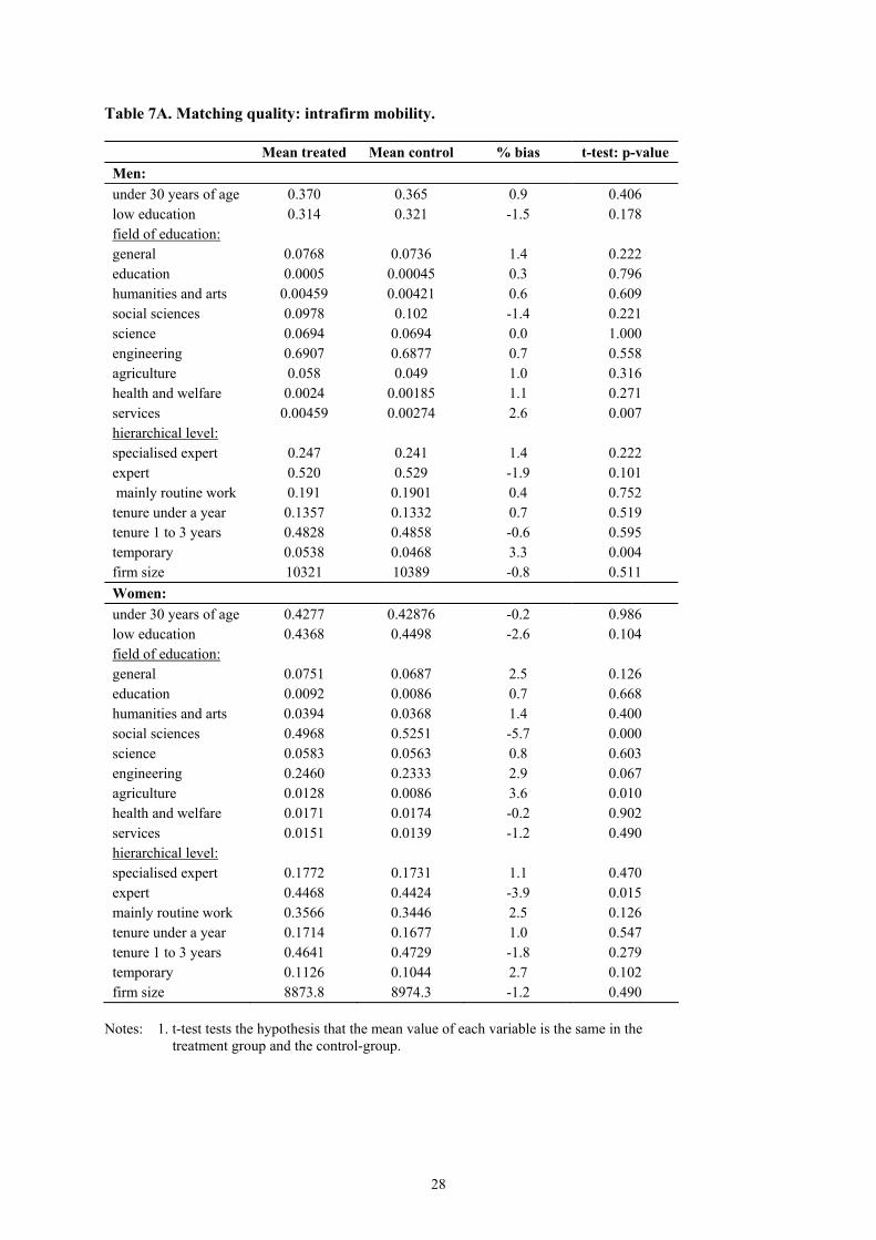
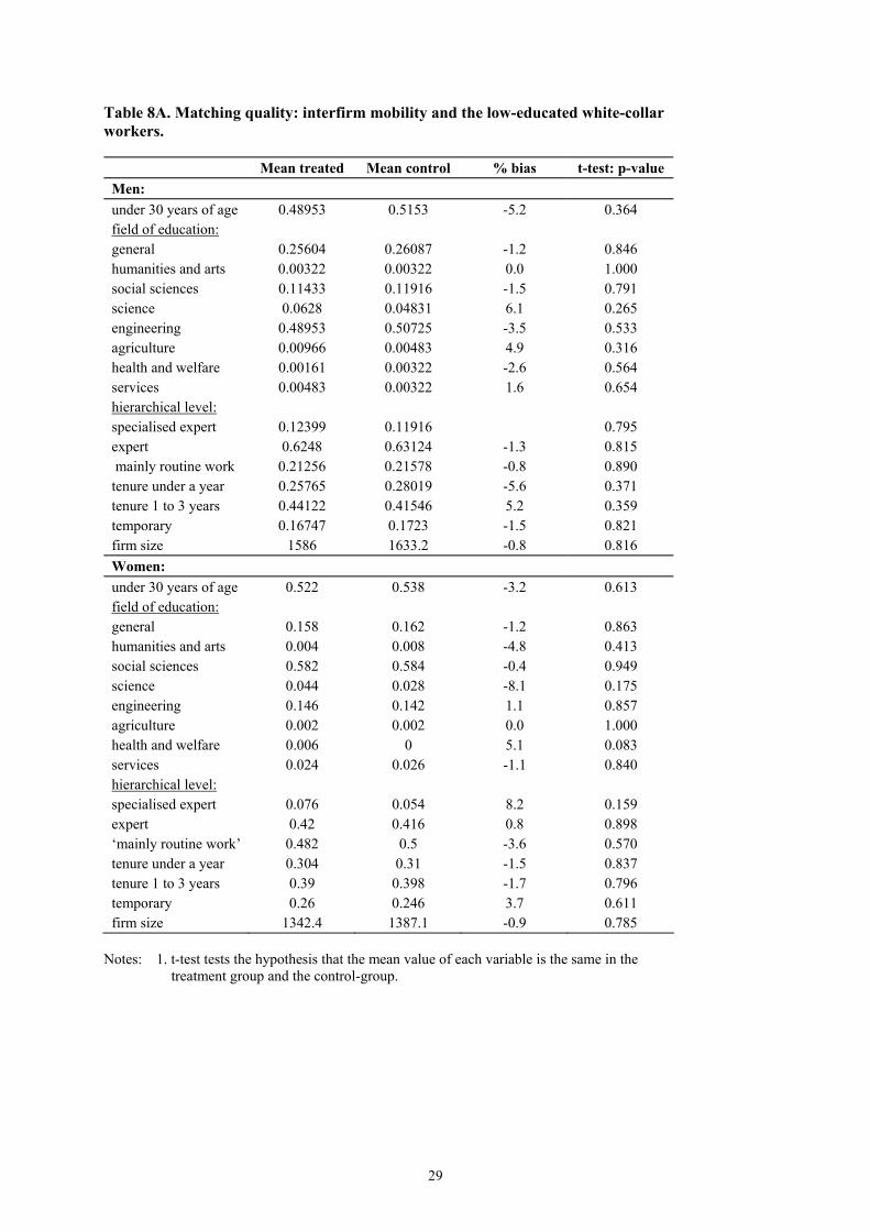
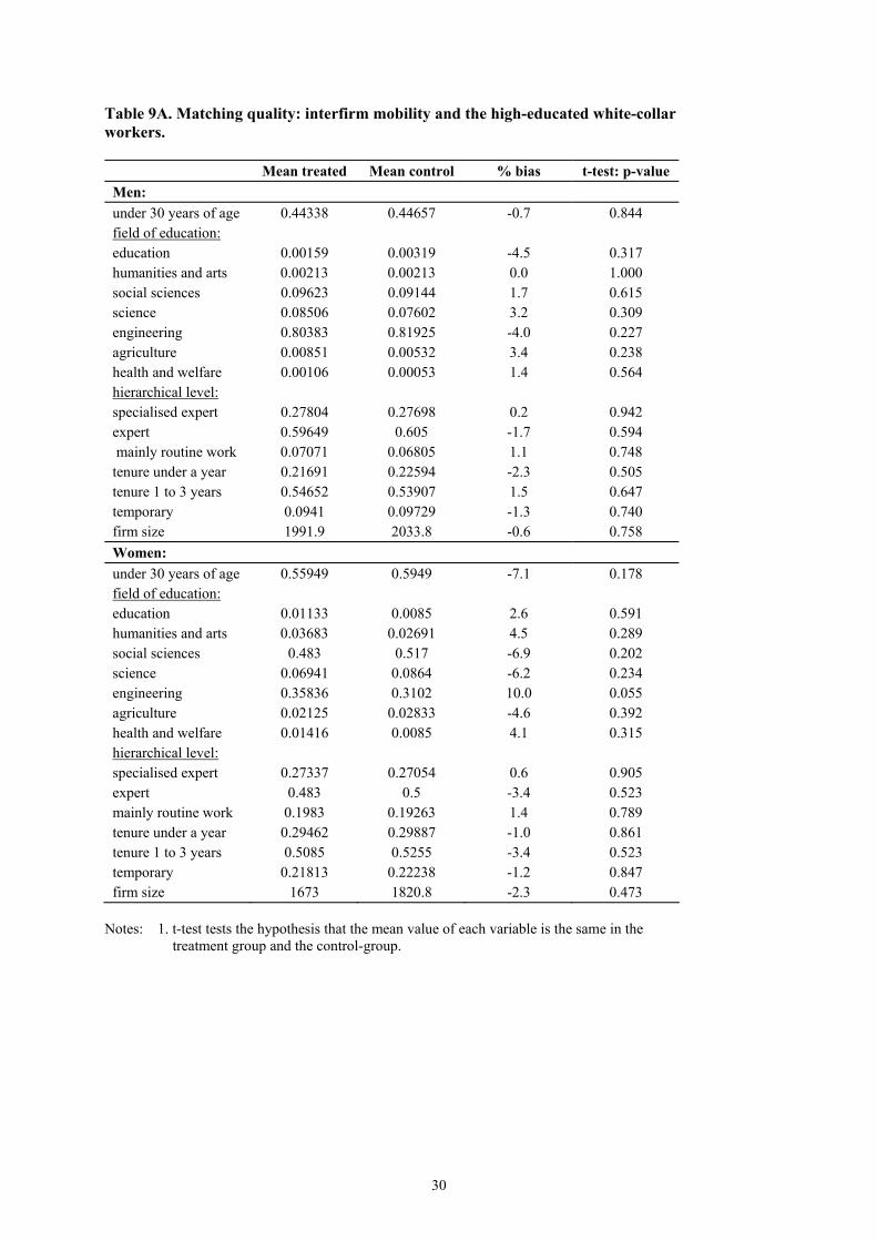
enough the importance of the matching quality. Tables 6A to 11A in appendix provide information on
the differences in the background characteristics between treatment and control groups after matching
has taken place. Generally, matching seems to work well since for most variables the mean values do
not differ between the groups at the conventional significance levels. However, two remarks should
be made. First, the matching quality is better for interfirm mobility where the difference in mean
values is insignificant for all variables at the 5 % level. This holds irrespective of gender or education
level. Second, the relatively weaker matching quality for intrafirm mobility is more of an issue for the
high-educated white-collar workers. But also here one should notice that the matching quality is
reasonable good: for the high-educated men, there are only two variables where the difference in
mean values is significant at the 5 % level while for the high-educated women, there are three such
variables.
5.2 Wage Effects of Interfirm Mobility
Table 3 presents the PSM-DID estimation results for interfirm mobility. The first two columns show
that male white-collar workers benefit more from employer changes than their female colleagues. For
men, the estimated wage premium to employer changes is 6.3 per cent meaning that men’s wage
growth is 6.3 per cent higher with a firm change compared to the case they had stayed in the same job
and in the same firm. The corresponding figure for women is 5.1 per cent.
The descriptive analysis in Section 3.2 suggests that there are significant differences in the wage
effects of mobility between educational levels, especially for women. Columns 3-6 in Table 3 provide
further evidence of the importance of accounting for this across educational level variation in the
returns to mobility when analyzing gender differences in the wage effects of mobility. As can be seen,
the low-educated women benefit considerably less from interfirm mobility than the high-educated
women or men. The wage premium to firm changes is 3.7 per cent for the low-educated women
compared to 6.4 per cent for the high-educated women who benefit similarly to the high-educated
men while there is a staggering 2.3 percentage points gender gap in the premium among the low-
educated white-collar workers.
Although a detailed investigation of the factors contributing to the lower returns to firm changes for
the low-educated women is beyond the scope of our paper, the issue nevertheless deserves some
discussion. One potential explanation is that the reasons for firm changes differ between the low-
educated women and other workers. Some studies have found evidence that women are in general

15
more likely than men to quit for family-related reasons and that these differences in the causes of
mobility explain at least part of the gender gap in the returns to mobility (e.g. Keith and McWilliams,
1997). It might well be that it is the low-educated women in particular who differ from the other
workers in motives for firm changes. Perhaps these women are less career-oriented and put less
weight on the pecuniary aspects of jobs while the high-educated women are more similar to men in
terms of factors behind employer changes.
Table 3. The wage effects of interfirm mobility by gender and educational level. Women Men Women Men Low education High education Low education High education PSM-DID 0.051 0.063 0.037 0.064 0.060 0.063 estimate (0.0047) (0.003) (0.007) (0.0068) (0.008) (0.004) N
49565
97769
25925
23640
32541
65225
Notes: 1. The results are based on a propensity score matching difference-in-differences method.
2. Bootstrapped standard errors are in parenthesis. 3. About the controlled variables, see e.g. Table 2A in appendix.
Our estimates of the returns to interfirm mobility seem to somewhat lower than what is typically
found in the literature. For example, several studies from the US and the UK document that employer
changes result in around ten per cent increase in wages (e.g. Keith and McWilliams, 1999; Campbell,
2001). There are undoubtedly many factors influencing to these differences in the returns to mobility
between Finland and the Anglo-Saxon countries, but one potentially important issue is the different
institutional set-ups discussed in Section 2. In particular, the history of centralized wage setting has
contributed to lower interfirm wage differentials in Finland compared the US and the UK decreasing
the potential gains from employer changes in the Finnish labour market.
5.3 Wage Effects of Intrafirm Mobility
Table 4 shows the corresponding results for intrafirm mobility. Job changes seem to be beneficial to
white-collar workers also when mobility takes place within a firm although the returns are smaller
than the gains from interfirm mobility. Furthermore, unlike in employer changes, there is no gender
gap in returns to within-firm mobility (columns 1 and 2). Both men and women experience on
average 2.8 per cent higher wage growth when they change jobs within a firm compared to the case
they had stayed in their current jobs.
Similar to employer changes, also here distinguishing between the low-educated and the high-
educated white-collar workers provides additional information on gender differences in returns to

16
mobility, although the variation in the premiums to job changes between educational levels is smaller
with intrafirm mobility than with employer changes. The low-educated women experience 0.6
percentage points lower return to within-firm job changes than the low-educated men while among
the high-educated white-collar workers women benefit more from mobility than men.
Table 4. The wage effects of intrafirm mobility by gender and educational level. Women Men Women Men Low education High education Low education High education PSM-DID 0.0278 0.0280 0.023 0.027 0.029 0.024 estimate (0.002) (0.002) (0.0025) (0.0068) (0.003) (0.002) N
56037
110941
28779
27258
36849
74089
Notes: 1. The results are based on a propensity score matching difference-in-differences method.
2. Bootstrapped standard errors are in parenthesis. 3. About the controlled variables, see e.g. Table 2A in appendix.
Also our estimates of the returns to internal mobility are somewhat lower compared to many of the
earlier studies who find significant wage premiums for within firm job changes, the estimates ranging
from 5 per cent to 15 per cent or even higher (Baker et al., 1994; McCue, 1996; Pergamit and Veum,
1999). Again, at least part of this difference in the estimated returns to mobility between our paper
and the earlier studies might be due to country differences in the institutional frameworks. Another
explaining factor is the differences in the types of job changes investigated. Most of the earlier studies
focus exclusively on promotions. Our measure of the within firm job changes on the other hand
includes also demotions and lateral movements in the firm’s organizational structure.
5.4 Robustness Checks
This section focuses on the sensitivity of our results with respect to the matching and estimation
methods used. As discussed in Section 4, we apply the nearest neighbour matching to match treatment
and control groups. This method guarantees a large number of matched pairs since all the treated units
are forced to find at least one match. However, the obvious drawback with the nearest neighbour
matching is that it may result in poor matches in some cases. One solution to overcome this problem
is to use Kernel matching instead. Kernel matching uses weighted averages of all individuals in the
control group to form matches with the treated. The weights are inversely proportional to the gap in
the propensity scores between the treated and controls, i.e. matches with better quality get higher
weights.

17
Tables 12A and 13A show the Kernel matching results for interfirm mobility and intrafirm job
changes, respectively. When compared to the nearest neighbour matching results presented in Tables
3 and 4, one can see that they are very similar. The Kernel matching produces somewhat larger
estimates of the returns to mobility, but all the main conclusions concerning the variation of wage
premium to mobility by gender, education and type of mobility remain the same. We thus conclude
that our findings are not driven by the choice of matching method.
Tables 14A and 15A show the OLS and fixed effects estimation results. As can be seen, also these
more conventional estimation methods support the main findings from the PSM-DID estimations.
6. CONCLUSIONS
This paper investigates gender differences in the returns to mobility using a large linked employer-
employee data on white-collar workers employed in the Finnish manufacturing over the period 1997-
2006. A novel feature of our paper is that it distinguishes between job changes within firms and
mobility between firms. We also differ from the earlier literature by investigating mobility and wage
growth by the level of education. The wage premiums to mobility are estimated using a propensity
score matching combined with the differences-in-differences method. This technique provides a way
to deal with both the unobserved heterogeneity problem and the endogeneity of mobility caused by
the simultaneity of job changes and wage growth.
Our results show that in order to understand gender differences in the returns to mobility, it is
important to give a closer look at the different types of job changes instead of investigating only the
overall separation rates. First, we observe that both kinds of mobility boost wage growth, but the
wage premium is much higher for interfirm mobility than for job changes taking place within a firm.
Also the gender gap in the returns to mobility varies considerable with the type of job changes, the
gap being 1.2 percentage points with mobility between firms and non-existent when mobility within
firms is considered. The returns to mobility differ also between educational levels. The low-educated
women benefit in general less from mobility than the high-educated women. This gap in returns is
particularly evident in firm changes. The low-educated men, on the other hand, benefit roughly the
same from mobility than the high-educated men.

18
REFERENCES
Abbott, Michael G., and Charles M. Beach (1994): “Wage Changes and Job Changes of Canadian
Women: Evidence from the 1986-87 Labour Market Activity Survey”, Journal of Human Resources,
Vol. 29(2), pp. 429-60.
Altonji, Joseph G., and Robert A. Shakotko (1987): “Do Wages Rise with Job Seniority?”, Review of
Economic Studies, Vol. 54(3), pp. 437-59.
Antel, John J. (1991): “The Wage Effects of Voluntary Labor Mobility with and without Intervening
Unemployment”, Industrial and Labor Relations Review, Vol. 44(2), pp. 299-306.
Asplund, Rita (2007): “Finland: Decentralisation Tendencies within a Collective Wage Bargaining
System”, ETLA Discussion papers No. 1077.
Baker, George, Michael Gibbs, and Bengt Holmstrom (1994): “The Internal Economics of the Firm:
Evidence from Personnel Data”, Quarterly Journal of Economics, Vol. 109(4), pp. 881-919.
Baker, George, and Bengt Holmstrom (1995): “Internal Labor Markets: Too many Theories, Too Few
Facts”, American Economic Review, Vol. 85(2), pp. 255-59.
Becker, Sascha O., and Andrea Ichino (2002): “Estimation of Average Treatment Effects Based on
Propensity Scores”, The Stata Journal, Vol. 2(4), pp. 358-7.
Blau, Francine D., and Lawrence M. Kahn (1981): “Race and Sex Differences in Quits by Young
Workers”, Industrial and Labor Relations Review, Vol. 34(4), pp. 563-77.
Blau, Francine, and Lawrence Kahn (1996): “Wage Structure and Gender Earnings Differentials: An
International Comparison”, Economica, Vol. 63(250), pp. S29-S62.
Blundell, Richard, and Monica Costa Dias (2002): “Alternative Approaches to Evaluation in
Empirical Microeconomics”, cemmap working paper CWP10/02.
Booth, Alison L., and Marco Francesconi (2000): “Job Mobility in 1990s Britain: Does Gender
Matter?”, Research in Labor Economics, Vol. 19, pp. 173-89.
Burdett, Kenneth (1978): “A Theory of Employee Job Search and Quit Rates”, American Economic
Review, Vol. 68(1), pp. 212-20.
Campbell, David (2001): “Estimating the Wage Effects of Job Mobility in Britain”, University of
Kent, Studies in Economics series, No. 0117.
Davia, Maria A. (2006): “Studying the Impact of Job Mobility on Wage Growth at the Beginning of
the Employment Career in Spain”, unpublished working paper.
Dustmann, Christian, and Sonia C. Pereira (2008): “Wage Growth and Job Mobility in the United
Kingdom and Germany”, Industrial and Labor Relations Review, Vol. 61(3), pp. 374-393.
19
Felmlee, Diana H. (1982): “Women’s Job Mobility Processes Within and Between Employers”,
American Sociological Review, Vol. 47(1), pp. 142-51.
Flinn, Christopher J. (1986): “Wages and Job Mobility of Young Workers”, Journal of Political
Economy, Vol. 94(3), pp. S88-S110.
Gangl, Markus (2003): “The Only Way is Up? Employment Protection and Job Mobility among
Recent Entrants to European Labour Markets”, European Sociological Review, Vol. 19(5), pp. 429-
49.
Gottschalk, Peter (2002): “Wage Mobility Within and Between Jobs”, Boston College Working
Papers in Economics, No. 486.
le Grand, Carl, and Michael Tåhlin (2002): “Job Mobility and Earnings Growth”, European
Sociological Review, Vol. 18(4), pp. 381-400.
Gregg, Paul, and Alan Manning (1997): “Labour Market Regulation and Unemployment”, in Snower
D.J., and G. de la Dehesa (eds) Unemployment Policy, Cambridge: Cambridge University Press, pp.
395-419.
Johnson, William R. (1978): “A Theory of Job Shopping”, Quarterly Journal of Economics, Vol.
92(2), pp. 261-78.
Jovanovic, Boyan (1979a): “Job Matching and the Theory of Turnover”, Journal of Political
Economy, Vol. 87(5), pp. 972-90.
Jovanovic, Boyan (1979b): “Firm-Specific Capital and Turnover”, Journal of Political Economy, Vol.
87(6), pp. 1246-59.
Kangasniemi, Mari (2003): “Essays on Job Tenure, Wages, Worker Mobility and Occupation in
Finnish Manufacturing: Do Institutions Matter?”, PhD-thesis, University of Essex.
Keith, Kirsten, and Abigail McWilliams (1997): “Job Mobility and Gender-Based Wage Growth
Differentials”, Economic Inquiry, Vol. 35(2), pp. 320-33.
Keith, Kirsten, and Abigail McWilliams (1999): “The Returns to Mobility and Job Search by
Gender”, Industrial and Labor Relations Review, Vol. 52(3), pp. 460-77.
Light, Audrey, and Manuelita Ureta (1992): “Panel Estimates of Male and Female Job Turnover
Behavior: Can Female Nonquitters Be Identied?”, Journal of Labor Economics, Vol. 10(2), pp. 156-
81.
Lillard, Lee A. (1999): “Job Turnover Heterogeneity and Person-Job-Specific Time-Series Wages”,
Annales d’Economie et de Statistique, iss. 55-56, pp. 183-210.
Loprest, Pamela J. (1992): “Gender Differences in Wage Growth and Job Mobility”, American
Economic Review, Vol. 82(2), pp. 526-32.
20
Manning, Alan (2003): “Monopsony in Motion: Imperfect Competition in Labor Markets”, Princeton:
Princeton University Press.
Manning, Alan, and Joanna Swaffield (2008): “The Gender Gap in Early-Career Wage Growth”,
Economic Journal, Vol. 118(530), pp. 983-1024.
McCue, Kristin (1996): “Promotions and Wage Growth”, Journal of Labor Economics, Vol. 14(2),
pp. 175-209.
Mincer, Jacob, and Boyan Jovanovic (1981): “Labor Mobility and Wages”, in Studies in Labor
Markets, edited by Sherwin Rosen, Chicago: University of Chicago Press.
Napari, Sami (2007): “Is There a Motherhood Wage Penalty in the Finnish Private Sector?”, ETLA
Discussion papers No. 1107.
Napari, Sami (2009): “Gender Differences in Early-Career Wage Growth”, Labour Economics, Vol.
16(2), pp. 140-58.
OECD (2004): “OECD Employment Outlook 2004”, Paris: OECD.
Pavlopoulos, Dimitris, Didier Fouarge, Ruud Muffels, and Jeroen K. Vermunt (2007: “Job Mobility
and Wage Mobility of High- and Low-Paid Workers”, Journal of Applied Social Science Studies,
Vol. 127(1), pp. 47-58.
Pergamit, Michael, and Jonathan R. Veum (1999): “What is a Promotion?”, Industrial and Labor
Relations Review, Vol. 52(4), pp. 581-601.
Pylkkänen, Elina, and Nina Smith (2004): ‘The Impact of Family-Friendly Policies in Denmark and
Sweden on Mothers’ Career Interruptions due to Childbirth’, IZA Discussion Paper No. 1050.
Rosenbaum, P.R., and D.B. Rubin (1983): “The Central Role of Propensity Score in Observational
Studies for Causal Effects”, Biometrika, Vol. 70(1), pp. 41-55.
Royalty, Anne Beeson (1998): “Job-to-Job and Job-to-Nonemployment Turnover by Gender and
Education Level”, Journal of Labor Economics, Vol. 16(2), pp. 392-443.
Sicherman, Nachum (1996): “Gender Differences in Departures from a Large Firm”, Industrial and
Labor Relations Review, Vol. 49(3), pp. 484-505.
Simpson, Wayne (1990): “Starting Even? Job Mobility and the Wage Gap Between Young Single
Males and Females”, Applied Economics, Vol. 22(6), pp. 723-37.
Teulings, Coen, and Joop Hartog (1998): “Corporatism or Competition? Labour Contracts,
Institutions and Wage Structures in International Comparison”, Cambridge: Cambridge University
Press.
Topel, Robert H. (1991): “Specific Capital, Mobility, and Wages: Wages Rise with Job Seniority”,
Journal of Political Economy, Vol. 99(1), pp. 145-76.

21
Topel, Robert H., and Michael P. Ward (1992): “Job Mobility and the Careers of Young Men”,
Quarterly Journal of Economics, Vol. 107(2), pp. 439-79.
Vartiainen, Juhana (1998): “The Labour Market in Finland: Institutions and Outcomes”, Prime
Minister’s Office, Publications Series 1998/2.
Viscusi, W. Kip (1980): “Sex Differences in Worker Quitting”, Review of Economics and Statistics,
Vol. 62(3), pp. 388-98.

22
APPENDIX
Table 1A. Summary statistics by gender and mobility status. Women Men Non-
movers Intra firm
movers
Inter firm
movers
Total Non-movers
Intra firm
movers
Inter firm
movers
Total
under 30 years old 42.5 42.8 54.4 42.8 37.6 37.0 45.6 37.7 30 years or older 57.5 57.2 45.6 57.2 62.4 63.0 54.4 62.3 low-educated 52.6 43.7 41.4 51.1 33.5 31.5 24.9 33.0 high-educated 47.4 56.3 58.6 48.9 66.5 68.5 75.1 67.0 general education 6.4 7.5 6.6 6.5 6.6 7.7 6.4 6.7 educational science 0.7 0.9 0.7 0.7 0.1 0.1 0.1 0.1 humanities and arts 3.6 3.9 2.3 3.6 0.4 0.5 0.2 0.4 social sciences 46.6 49.7 52.4 47.1 8.6 9.8 10.1 8.8 natural sciences 6.3 5.8 5.8 6.2 7.5 6.9 8.0 7.4 technology 27.2 24.6 27.0 26.9 71.6 69.1 72.5 71.3 agriculture 1.6 1.3 1.3 1.5 0.9 0.6 0.9 0.9 health and welfare 2.4 1.7 1.1 2.3 0.3 0.2 0.1 0.3 services 2.3 1.5 1.3 2.2 0.5 0.5 0.2 0.5 management 1.8 5.4 5.3 2.3 3.3 11.2 8.0 4.5 specialised experts 17.3 31.6 21.9 19.3 27.2 44.3 30.6 29.6 experts 44.2 43.6 46.5 44.2 57.5 38.5 53.5 54.8 routine work 36.8 19.5 26.2 34.2 12.0 5.9 7.8 11.1 lag (tenure under a year) 16.1 17.1 29.7 16.5 15.2 13.6 22.8 15.2 lag (tenure 1-3 years) 41.6 46.4 46.0 42.4 44.6 48.3 52.0 45.3 lag (tenure over 3 years) 42.3 36.4 24.4 41.1 40.2 38.1 25.2 39.6 temporary 5.9 13.1 5.6 6.0 2.1 4.1 1.7 2.1 firm size 5067.9 9299.2 2334.5 5578.3 6920.6 10800.8 2410.7 7357.9

23
Table 2A. Probit estimation results for interfirm mobility.
Men Women
under 30 years old -0.047 (0.020)
0.011 (0.028)
low education -0.235***
(0.024) -0.193***
(0.03) field of education:
general 0.11
(0.074) 0.098
(0.109)
education 0.177
(0.287) -0.093 (0.186)
humanities and arts -0.182 (0.180)
-0.182 (0.126)
social sciences 0.080
(0.072) 0.126
(0.099)
science 0.001
(0.074) -0.007 (0.111)
technology 0.019
(0.101) 0.019
(0.101)
agriculture 0.031
(0.0688) -0.203 (0.144)
health and welfare -0.142 (0.114)
-0.352 (0.146)
services -0.125 (0.140)
-0.125 (0.140)
hierarchical level:
specialised expert• -0.149***
(0.045) -0.161***
(0.08)
expert• -0.126***
(0.043) -0.216***
(0.077)
mainly routine work• -0.222***
(0.079) -0.328 ***
(0.079)
tenure under a year• 0.220*** (0.028)
0.347*** (0.039)
tenure 1 to 3 years• 0.223*** (0.022)
0.232*** (0.032)
temporary work• 0.341*** (0.033)
0.308*** (0.033)
firm size• -0.00004*** (1.83e-06)
-0.00004*** (3.05e-06)
Notes: 1. Standard errors are in parenthesis.
2. ***: difference significant at 1 % level. 3. •: one year lag.

24
Table 3A. Probit estimation results for intrafirm mobility.
Men Women
under 30 years old -0.039***
(0.011) 0.008
(0.015)
low education -0.144***
(0.012) -0.177***
(0.016) field of education:
general 0.026
(0.029) 0.219*** (0.047)
education -0.274 (0.205)
0.069 (0.087)
humanities and arts -0.174***
(0.076) -0.066 (0.054)
social sciences -0.029 (0.029)
0.065 (0.041)
science -0.152***
(0.031) -0.082* (0.049)
technology -0.148***
(0.026) -0.051 (0.043)
agriculture -0.208***
(0.062) 0.015
(0.070)
health and welfare -0.157 (0.096)
-0.037 (0.063)
services -0.104 (0.072)
-0.105 (0.064)
hierarchical level:
specialised expert• -0.245***
(0.026) -0.145***
(0.051)
expert• -0.159***
(0.026) -0.091* (0.05)
mainly routine work• 0.282*** (0.029)
0.025 (0.05)
tenure under a year• 0.019
(0.016) 0.07*** (0.022)
tenure 1 to 3 years• 0.062*** (0.011)
0.045*** (0.016)
temporary• 0.265*** (0.023)
0.191*** (0.023)
firm size• 0.00003*** (5.72e-07)
0.00003*** (8.56e-07)
Notes: 1. Standard errors are in parenthesis.
2. ***: difference significant at 1 % level, *: difference significant at 10 % level. 3. •: one year lag.

25
Table 4A. Probit estimation results for interfirm mobility by educational level.
Low-educated High-educated Men Women Men Women
under 30 years old 0.020
(0.038) 0.004
(0.042) -0.015 (0.024)
0.021 (0.038)
field of education:
general 0.112
(0.075) 0.217
(0.047) - -
education - 0.073
(0.086) 0.368
(0.504) 0.124
(0.272)
humanities and arts -0.055 (0.291)
-0.06 (0.054)
-0.059 (0.466)
0.024 (0.235)
social sciences 0.014
(0.083) 0.063
(0.041) 0.291
(0.419) 0.301
(0.222)
science 0.065
(0.095) -0.079 (0.049)
0.155 (0.419)
0.103 (0.229)
technology 0.062
(0.071) -0.049 (0.043)
0.195 (0.418)
0.224 (0.223)
agriculture -0.048 (0.182)
0.024 (0.070)
-0.018 (0.432)
-0.008 (0.108)
health and welfare -0.445 (0.349)
-0.026 (0.063)
-0.011 (0.507)
-0.108 (0.254)
services -0.420* (0.215)
-0.102 (0.064)
0.188 (0.532)
organizational hierarchical level:
specialised expert• -0.264** (0.105)
-0.472*** (0.165)
-0.121** (0.050)
-0.078 (0.091)
expert• -0.272***
(0.097) -0.425***
(0.154) -0.089* (0.048)
-0.156* (0.089)
mainly routine work• -0.387***
(0.029) -0.546***
(0.153) -0.159***
(0.061) -0.248***
(0.094)
tenure under a year• 0.265*** (0.052)
0.432*** (0.057)
0.197*** (0.033)
0.270*** (0.054)
tenure 1 to 3 years• 0.209*** (0.041)
0.261*** (0.047)
0.223*** (0.026)
0.192*** (0.046)
temporary• 0.315*** (0.054)
0.302*** (0.052)
0.353*** (0.042)
0.312*** (0.048)
firm size• -0.00004*** (3.97e-06)
-0.00004*** (5.59e-06)
-0.00004*** (2.07e-06)
-0.00004*** (3.66e-06)
Notes: 1. Standard errors are in parenthesis.
2. ***: difference significant at 1 % level, **: difference significant at 5 % level, *: difference significant at 10 % level. 3. *: one year lag.

26
Table 5A. Probit estimation results for intrafirm mobility by educational level.
Low-educated High-educated Men Women Men Women
under 30 years old -0.0048 (0.019)
0.064*** (0.022)
-0.054*** (0.013)
-0.047** (0.021)
field of education:
general 0.075
(0.030) 0.217
(0.047) - -
education - 0.073
(0.086) -0.137 (0.239)
0.195 (0.141)
humanities and arts 0.038
(0.060) -0.06
(0.054) -0.043 (0.147)
0.025 (0.124)
social sciences 0.066
(0.035) 0.063
(0.041) 0.090
(0.124) 0.139
(0.119)
science -0.117 (0.045)
-0.079 (0.049)
-0.021 (0.124)
0.002 (0.123)
technology -0.039 (0.028)
-0.049 (0.043)
-0.031 (0.1228)
0.107 (0.120)
agriculture -0.178 (0.108)
0.024 (0.070)
-0.080 (0.140)
0.120 (0.133)
health and welfare -0.056 (0.124)
-0.026 (0.063)
-0.041 (0.189)
-0.032 (0.137)
services 0.070
(0.077) -0.102 (0.064)
- -
hierarchical level:
specialised expert• -0.231***
(0.062) -0.270** (0.107)
-0.252*** (0.029)
-0.109* (0.059)
expert• -0.258***
(0.059) -0.304***
(0.103) -0.138***
(0.028) -0.025 (0.058)
mainly routine work• 0.038
(0.060) -0.263** (0.102)
0.488 (0.033)
0.241*** (0.060)
tenure under a year• 0.061** (0.028)
0.090*** (0.032)
-0.027 (0.020)
0.032 (0.031)
tenure 1 to 3 years• 0.063*** (0.019)
0.004*** (0.023)
0.042*** (0.013)
0.055** (0.022)
temporary• 0.324*** (0.034)
0.195*** (0.033)
0.228*** (0.032)
0.185*** (0.034)
firm size• 0.00004*** (1.07e-06)
-0.00004*** (1.38e-06)
0.00002*** (6.79e-07)
-0.00003*** (1.11e-06)
Notes: 1. Standard errors are in parenthesis.
2. ***: difference significant at 1 % level, **: difference significant at 5 % level, *: difference significant at 10 % level. 3. *: one year lag.

27
Table 6A. Matching quality: interfirm mobility.
Mean treated Mean control % bias t-test: p-value Men: under 30 years old 0.454 0.456 -0.3 0.910 low education 0.248 0.2402 1.8 0.511 field of education: general 0.0635 0.0651 -0.7 0.818 education 0.0012 0.008 1.3 0.655 humanities and arts 0.0024 0.004 -2.8 0.317 social sciences 0.1007 0.0995 0.4 0.888 science 0.0795 0.0667 4.8 0.082 technology 0.7258 0.7394 -3.0 0.278 agriculture 0.0879 0.0679 2.1 0.422 health and welfare 0.0012 0.004 1.7 0.317 services 0.002 0.0012 1.3 0.479 hierarchical level: specialised expert 0.2398 0.2366 1.3 0.791 expert 0.6035 0.6075 -1.1 0.772 mainly routine work 0.1059 0.1011 3.2 0.578
tenure under a year 0.2270 0.2234 -1.3 0.761 tenure 1 to 3 years 0.5203 0.5199 -1.7 0.977 temporary 0.1123 0.1103 0.8 0.822 firm size 1891.2 1943 -0.8 0.651 Women: under 30 years old 0.5439 0.5588 -3.0 0.461 low education 0.4145 0.4220 -1.5 0.710 field of education: general 0.0655 0.0696 -1.7 0.685 education 0.0066 0.0041 3.1 0.404 humanities and arts 0.0232 0.0223 0.5 0.892 social sciences 0.5240 0.5439 -4.0 0.327 science 0.0588 0.0530 2.4 0.535 technology 0.2703 0.2595 2.4 0.549 agriculture 0.0132 0.0116 1.4 0.713 health and welfare 0.0107 0.0074 2.5 0.392 services 0.0132 0.0141 -0.6 0.861 hierarchical level: specialised expert 0.1915 0.1865 1.3 0.755 expert 0.4568 0.4552 0.3 0.935 mainly routine work 0.3159 0.3233 -1.6 0.694
tenure under a year 0.2985 0.3151 -4.0 0.377 tenure 1 to 3 years 0.4593 0.4519 1.5 0.713 temporary 0.2354 0.2371 -0.5 0.924 firm size 1535.9 1686.6 -2.7 0.281
Notes: 1. t-test tests the hypothesis that the mean value of each variable is the same in the
treatment group and the control-group.
28
Table 7A. Matching quality: intrafirm mobility.
Mean treated Mean control % bias t-test: p-value Men: under 30 years of age 0.370 0.365 0.9 0.406 low education 0.314 0.321 -1.5 0.178 field of education: general 0.0768 0.0736 1.4 0.222 education 0.0005 0.00045 0.3 0.796 humanities and arts 0.00459 0.00421 0.6 0.609 social sciences 0.0978 0.102 -1.4 0.221 science 0.0694 0.0694 0.0 1.000 engineering 0.6907 0.6877 0.7 0.558 agriculture 0.058 0.049 1.0 0.316 health and welfare 0.0024 0.00185 1.1 0.271 services 0.00459 0.00274 2.6 0.007 hierarchical level: specialised expert 0.247 0.241 1.4 0.222 expert 0.520 0.529 -1.9 0.101 mainly routine work 0.191 0.1901 0.4 0.752 tenure under a year 0.1357 0.1332 0.7 0.519 tenure 1 to 3 years 0.4828 0.4858 -0.6 0.595 temporary 0.0538 0.0468 3.3 0.004 firm size 10321 10389 -0.8 0.511 Women: under 30 years of age 0.4277 0.42876 -0.2 0.986 low education 0.4368 0.4498 -2.6 0.104 field of education: general 0.0751 0.0687 2.5 0.126 education 0.0092 0.0086 0.7 0.668 humanities and arts 0.0394 0.0368 1.4 0.400 social sciences 0.4968 0.5251 -5.7 0.000 science 0.0583 0.0563 0.8 0.603 engineering 0.2460 0.2333 2.9 0.067 agriculture 0.0128 0.0086 3.6 0.010 health and welfare 0.0171 0.0174 -0.2 0.902 services 0.0151 0.0139 -1.2 0.490 hierarchical level: specialised expert 0.1772 0.1731 1.1 0.470 expert 0.4468 0.4424 -3.9 0.015 mainly routine work 0.3566 0.3446 2.5 0.126 tenure under a year 0.1714 0.1677 1.0 0.547 tenure 1 to 3 years 0.4641 0.4729 -1.8 0.279 temporary 0.1126 0.1044 2.7 0.102 firm size 8873.8 8974.3 -1.2 0.490
Notes: 1. t-test tests the hypothesis that the mean value of each variable is the same in the
treatment group and the control-group.
29
Table 8A. Matching quality: interfirm mobility and the low-educated white-collar workers.
Mean treated Mean control % bias t-test: p-value Men: under 30 years of age 0.48953 0.5153 -5.2 0.364 field of education: general 0.25604 0.26087 -1.2 0.846 humanities and arts 0.00322 0.00322 0.0 1.000 social sciences 0.11433 0.11916 -1.5 0.791 science 0.0628 0.04831 6.1 0.265 engineering 0.48953 0.50725 -3.5 0.533 agriculture 0.00966 0.00483 4.9 0.316 health and welfare 0.00161 0.00322 -2.6 0.564 services 0.00483 0.00322 1.6 0.654 hierarchical level: specialised expert 0.12399 0.11916 0.795 expert 0.6248 0.63124 -1.3 0.815 mainly routine work 0.21256 0.21578 -0.8 0.890 tenure under a year 0.25765 0.28019 -5.6 0.371 tenure 1 to 3 years 0.44122 0.41546 5.2 0.359 temporary 0.16747 0.1723 -1.5 0.821 firm size 1586 1633.2 -0.8 0.816 Women: under 30 years of age 0.522 0.538 -3.2 0.613 field of education: general 0.158 0.162 -1.2 0.863 humanities and arts 0.004 0.008 -4.8 0.413 social sciences 0.582 0.584 -0.4 0.949 science 0.044 0.028 -8.1 0.175 engineering 0.146 0.142 1.1 0.857 agriculture 0.002 0.002 0.0 1.000 health and welfare 0.006 0 5.1 0.083 services 0.024 0.026 -1.1 0.840 hierarchical level: specialised expert 0.076 0.054 8.2 0.159 expert 0.42 0.416 0.8 0.898 ‘mainly routine work’ 0.482 0.5 -3.6 0.570 tenure under a year 0.304 0.31 -1.5 0.837 tenure 1 to 3 years 0.39 0.398 -1.7 0.796 temporary 0.26 0.246 3.7 0.611 firm size 1342.4 1387.1 -0.9 0.785
Notes: 1. t-test tests the hypothesis that the mean value of each variable is the same in the treatment group and the control-group.
30
Table 9A. Matching quality: interfirm mobility and the high-educated white-collar workers.
Mean treated Mean control % bias t-test: p-value Men: under 30 years of age 0.44338 0.44657 -0.7 0.844 field of education: education 0.00159 0.00319 -4.5 0.317 humanities and arts 0.00213 0.00213 0.0 1.000 social sciences 0.09623 0.09144 1.7 0.615 science 0.08506 0.07602 3.2 0.309 engineering 0.80383 0.81925 -4.0 0.227 agriculture 0.00851 0.00532 3.4 0.238 health and welfare 0.00106 0.00053 1.4 0.564 hierarchical level: specialised expert 0.27804 0.27698 0.2 0.942 expert 0.59649 0.605 -1.7 0.594 mainly routine work 0.07071 0.06805 1.1 0.748 tenure under a year 0.21691 0.22594 -2.3 0.505 tenure 1 to 3 years 0.54652 0.53907 1.5 0.647 temporary 0.0941 0.09729 -1.3 0.740 firm size 1991.9 2033.8 -0.6 0.758 Women: under 30 years of age 0.55949 0.5949 -7.1 0.178 field of education: education 0.01133 0.0085 2.6 0.591 humanities and arts 0.03683 0.02691 4.5 0.289 social sciences 0.483 0.517 -6.9 0.202 science 0.06941 0.0864 -6.2 0.234 engineering 0.35836 0.3102 10.0 0.055 agriculture 0.02125 0.02833 -4.6 0.392 health and welfare 0.01416 0.0085 4.1 0.315 hierarchical level: specialised expert 0.27337 0.27054 0.6 0.905 expert 0.483 0.5 -3.4 0.523 mainly routine work 0.1983 0.19263 1.4 0.789 tenure under a year 0.29462 0.29887 -1.0 0.861 tenure 1 to 3 years 0.5085 0.5255 -3.4 0.523 temporary 0.21813 0.22238 -1.2 0.847 firm size 1673 1820.8 -2.3 0.473
Notes: 1. t-test tests the hypothesis that the mean value of each variable is the same in the
treatment group and the control-group.

31
Table 10A. Matching quality: intrafirm mobility and the low-educated white-collar workers.
Mean treated Mean control % bias t-test: p-value Men: under 30 years of age 0.39112 0.38118 2.0 0.311 field of education: general 0.24412 0.23601 2.0 0.346 education 0.00243 0.00264 -0.4 0.841 social sciences 0.11415 0.11638 -0.7 0.729 science 0.04542 0.04319 1.0 0.590 engineering 0.42559 0.43917 -2.7 0.173 agriculture 0.00487 0.00162 3.8 0.005 health and welfare 0.00446 0.00264 2.6 0.128 services 0.01237 0.01075 1.4 0.451 hierarchical level: specialised expert 0.17336 0.16464 2.4 0.248 expert 0.50284 0 .52251 -4.0 0.051 mainly routine work 0.30109 0.28731 3.1 0.133 tenure under a year 0.15673 0.15004 1.8 0.357 tenure 1 to 3 years 0.44546 0.45337 -1.6 0.430 temporary 0.08556 0.07664 3.4 0.105 firm size 9727.8 9882 -1.9 0.400 Women: under 30 years of age 0.4198 0.41473 1.0 0.674 field of education: general 0.17203 0.16219 2.8 0.280 education 0.0003 0.0003 0.0 1.000 humanities and arts 0.00805 0.00835 -0.3 0.892 social sciences 0.55098 0.55963 -1.7 0.476 science 0.04085 0.04025 0.3 0.901 engineering 0.11002 0.11181 -0.5 0.816 agriculture 0.00298 0.00298 0.0 1.000 health and welfare 0.01998 0.02236 -1.7 0.497 hierarchical level:: specialised expert 0.09839 0.08974 3.0 0.225 expert 0.39535 0.39624 -0.2 0.940 mainly routine work 0.4952 0.5059 -2.1 0.379 tenure under a year 0.169 0.161 2.4 0.341 tenure 1 to 3 years 0.3849 0.3855 -0.1 0.960 temporary 0.1267 0.1136 4.1 0.099 firm size 10096 10201 -1.2 0.592
Notes: 1. t-test tests the hypothesis that the mean valua of each variable is the same in the
treatment group and the control-group.

32
Table 11A. Matching quality: intrafirm mobility and the high-educated white-collar workers.
Mean treated Mean control % bias t-test: p-value Men: under 30 years of age 0.3603 0.3577 0.5 0.691 field of education: education 0.0007 0.0015 -2.6 0.102 humanities and arts 0.0055 0.008 -3.46 0.031 social sciences 0.0903 0.0896 0.3 0.849 science 0.0805 0.0817 -0.4 0.745 engineering 0.8124 0.8084 1.0 0.454 agriculture 0.0062 0.0061 0.1 0.931 health and welfare 0.0015 0.0026 -2.8 0.07 hierarchical level: specialised expert 0.2813 0.2797 0.3 0.796 expert 0.5284 0.5413 -2.6 0.057 mainly routine work 0.1418 0.1308 3.7 0.019 tenure under a year 0.1261 0.1287 -0.8 0.567 tenure 1 to 3 years 0.4999 0.505 -1.1 0.421 temporary 0.0392 0.0376 0.9 0.567 firm size 10321 10389 -0.8 0.511 Women: under 30 years of age 0.43386 0.43802 -0.8 0.696 field of education: education 0.0162 0.0132 2.5 0.245 humanities and arts 0.0638 0.0668 -1.2 0.572 social sciences 0.4549 0.4815 -5.4 0.013 science 0.0719 0.0682 1.3 0.500 engineering 0.3515 0.3383 2.7 0.197 agriculture 0.0206 0.0136 4.5 0.013 health and welfare 0.0150 0.0134 1.1 0.525 hierarchical level:: specialised expert 0.2384 0.2345 0.9 0.667 expert 0.4868 0.5099 -4.6 0.032 ‘mainly routine work’ 0.2490 0.2319 4.2 0.063 tenure under a year 0.1727 0.1653 1.9 0.359 tenure 1 to 3 years 0.5256 0.5430 -3.5 0.106 temporary 0.1017 0.098 1.3 0.542 firm size 10096 10201 -1.2 0.592
Notes: 1. t-test tests the hypothesis that the mean value of each variable is the same in the
treatment group and the control-group.

33
Table 12A. The wage effects of interfirm mobility by gender and educational level – kernel matching. Women Men
Women Men Low education High education Low education High education
PSM-DID 0.058 0.0724 0.045 0.067 0.072 0.072 estimate (0.0038) (0.0024) (0.0049) (0.0044) (0.0075) (0.0029)
Notes: 1. The results are based on a propensity score matching difference-in-differences method.
2. Bootstrapped standard errors are in parenthesis. 3. About the controlled variables, see e.g. Table 2A in appendix.
Table 13A. The wage effects of intrafirm mobility by gender and educational level – kernel matching. Women Men
Women Men Low education High education Low education High education
PSM-DID 0.029 0.027 0.027 0.0286 0.0313 0.0262 estimate (0.0009) (0.0006) (0.0014) (0.0014) (0.0014) (0.0007)
Notes: 1. The results are based on a propensity score matching difference-in-differences method.
2. Bootstrapped standard errors are in parenthesis. 3. About the controlled variables, see e.g. Table 2A in appendix.
Table 14A. The wage effects of interfirm mobility by gender and educational level – OLS and fixed effects results Women Men
Women Men Low education High education Low education High education
OLS 0.052 0.067 0.0385 0.0620 0.0646 0.0672 (0.0035) (0.0027) (0.0051) (0.0047) (0.0062) (0.0029) Fixed effects 0.051 0.067 0.0348 0.060 0.058 0.0693 (0.0039) (0.0030) (0.0056) (0.0053) (0.0077) (0.0033)
Notes: 1. About the controlled variables, see e.g. Table 2A in appendix.
2. Robust standard errors with clustering on the individual are in parentheses.
Table 15A. The wage effects of intrafirm mobility by gender and educational level – OLS and fixed effects results Women Men
Women Men Low education High education Low education High education
OLS 0.0278 0.0269 0.0266 0.0285 0.0295 0.0253 (0.0010) (0.0007) (0.0015) (0.0013) (0.0015) (0.0008) Fixed effects 0.0229 0.0222 0.0208 0.0235 0.0219 0.0213 (0.0011) (0.0008) (0.0017) (0.0015) (0.0016) (0.0009)
Notes: 1. About the controlled variables, see e.g. Table 2A in appendix.
2. Robust standard errors with clustering on the individual are in parentheses.


