35
2ORIGIN OF BLACK BOXES
Statistics uses data to explore problems.
Think of the data as being generated by a blackbox .
A vector of input variables x (independentvariables) go into one side.
Response variables y come out on the other side.
Inside the black box, nature functions toassociate the input variables with the responsevariables, so the picture is like this:
All we see are a sample of data
(yn ,xn ) n =1,..., N )
From this, ststisticians want to draw conclusionsabout the mechanism operating inside the black box.

3STOCHASTIC DATA MODELING
starts with assuming a stochastic data model forthe inside of the black box.
A common data model is that data are generatedby independent draws from:
response variablesf(predictor variables,random noise, parameters)
Parameters are estimated from the data and themodel then used for information and/orprediction. The black box is filled in like this:
Model validation is yes-no using goodness-of-fittests and residual examination
Inferring a mechanism for the black box is a highlyrisky and ambiguous venture.
Nature's mechanisms are generally complex andcannot summarized by a relatively simple stochasticmodel, even as a first approximation. The attraction:a deceptively simple picture of the inside.

4FITTING THE DATA
An important principle
The better the model fits the data, the more soundthe inferences about the black box are.
Goodness-of-fit tests and residual analysis arenot reliable. They accept a multitude of badlyfitting models.
Suppose there is a model f (x)that outputs anestimate y of the true y for each value of x .
Then a measure of how well f fits the data isgiven by how close y is to y. This can bemeasured as follows: given an independent testset
(y' n ,x' n ) n =1,..., N' )
and a loss function L(y,y) , define the estimatedprediction error as
PE = avn.' L(yn' , f (xn'
' ))
If there is no test set, use cross-validation toestimate PE.
The lower the PE, the better the fit to the data
5RANDOM FORESTS
A random forest (RF) is a collection of tree predictors
f (x,T,Θk ), k =1,2,..., K )
where the Θk are i.i.d random vectors.
In regression, the forest prediction is unweightedaverage over the forest: in classification, theunweighted plurality.
Unlike boosting, the LLN insures convergence ask→∞.
The key to accuracy is low correlation and bias.To keep bias low, trees are grown to maximumdepth.
To keep correlation low, the current version usesthis randomization.
1) Each tree is grown on a bootstrap sample ofthe training set.
2) A number m is specified much smaller than thetotal number of variables M. At each node, mvariables are selected at random out of the M,and the split is the best split on these m variables.
(see Random Forests , Machine Learning(2001) 45 5-320)

6 RF AND OUT-OF-BAG (OOB)
In empirical tests, RF has proven to have lowprediction error. On a variety of data sets, it ismore accurate than Adaboost (see my paper)
It handles hundreds and thousands of inputvariables with no degeneration in accuracy
An important feature is that it carries along aninternal test set estimate of the predictionerror.
For every tree grown, about one-third of thecases are out-of-bag (out of the bootstrapsample). Abbreviated oob.
Put these oob cases down the corresponding treeand get response estimates for them.
For each case n, average or pluralize theresponse estimates over all time that n was oob toget a test set estimate yn for yn.
Averaging the loss over all n give the test setestimate of prediction error.
The only adjustable parameter in RF is m. Thedefault value for m is M . But RF is not sensitiveto the value of m over a wide range.

7 HAVE WE PRODUCED ONLY A GOLEM?
With scientific data sets more is required than anaccurate prediction, i.e. relevant information about the relation between the inputs and outputs and about the data--
looking inside the black box is necessary
Stochastic data modelers have criticized the machine learning efforts on the grounds that the accurate predictors constructed are so complex that it is nearly impossible to use them to get insights into the underlying structure of the data.
They are simply large bulky incoherent singlepurpose machines.
The contrary is true
Using RF we can get more reliable informationabout the inside of the black box than using anystochastic model.
But it is not in the form of simple equations.
8
RF & LOOKING INSIDE THE BLACK BOX
The design of random forests is to give the user agood deal of information about the data besidesan accurate prediction.
Much of this information comes from using theoob cases in the training set that have been leftout of the bootstrapped training set.
The information includes:
i) Variable importance measures
ii) Effects of variables on predictions
iii) Intrinsic proximities between cases
iv) Clustering
v) Scaling coordinates based on the proximities
vi) Outlier detection
I will explain how these work and giveapplications, both for labeled and unlabeled data.

9
VARIABLE IMPORTANCE.
Because of the need to know which variables areimportant in the classification, RF has threedifferent ways of looking at variable importance.
Sometimes influential variables are hard to spot--using these three measures provides moreinformation.
Measure 1
To estimate the importance of the mth variable, inthe oob cases for the kth tree, randomly permuteall values of the mth variable
Put these altered oob x-values down the treeand get classifications.
Proceed as though computing a new internalerror rate.
The amount by which this new error exceeds theoriginal test set error is defined as the importanceof the mth variable.

1 0
Measures 2 and 3
For the nth case in the data, its margin at the endof a run is the proportion of votes for its trueclass minus the maximum of the proportion ofvotes for each of the other classes.
The 2nd measure of importance of the mthvariable is the average lowering of the marginacross all cases when the mth variable israndomly permuted as in method 1.
The third measure is the count of how manymargins are lowered minus the number ofmargins raised.
We illustrate the use of this information by someexamples.
1 1AN EXAMPLE--HEPATITIS DATA
Data: survival or non survival of 155 hepatitispatients with 19 covariates.
Analyzed by Diaconis and Efron in 1983 ScientificAmerican.
The original Stanford Medical School analysisconcluded that the important variables werenumbers 6, 12, 14, 19.
Efron and Diaconis drew 500 bootstrap samplesfrom the original data set and used a similarprocedure, including logistic regression, to isolatethe important variables in each bootstrapped dataset.
Their conclusion , "Of the four variablesoriginally selected not one was selected in morethan 60 percent of the samples.
Hence the variables identified in the originalanalysis cannot be taken too seriously."
1 2
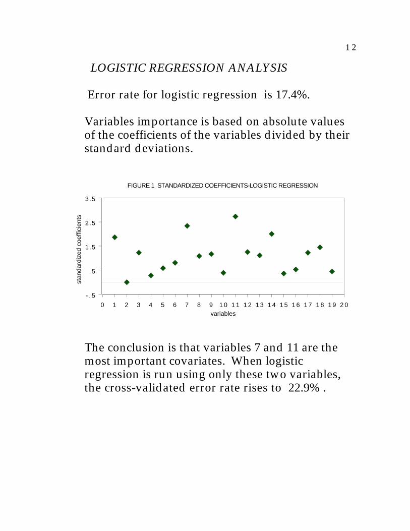
LOGISTIC REGRESSION ANALYSIS
Error rate for logistic regression is 17.4%.
Variables importance is based on absolute valuesof the coefficients of the variables divided by theirstandard deviations.
- . 5
.5
1.5
2.5
3.5
stan
dard
ized
coe
ffici
ents
0 1 2 3 4 5 6 7 8 9 1 0 1 1 1 2 1 3 1 4 1 5 1 6 1 7 1 8 1 9 2 0variables
FIGURE 1 STANDARDIZED COEFFICIENTS-LOGISTIC REGRESSION
The conclusion is that variables 7 and 11 are themost important covariates. When logisticregression is run using only these two variables,the cross-validated error rate rises to 22.9% .

1 3
ANALYSIS USING RF
The error rate is 12.3%--30% reduction from thelogistic regression error. Variable importances(measure 1) are graphed below:
- 1 0
0
1 0
2 0
3 0
4 0
5 0
perc
ent i
ncre
se in
err
or
0 1 2 3 4 5 6 7 8 9 1 0 1 1 1 2 1 3 1 4 1 5 1 6 1 7 1 8 1 9 2 0
variables
FIRURE 2 VARIABLE IMPORTANCE-RANDOM FOREST
Two variables are singled out--the 12th and the17th The test set error rates running 12 and 17alone were 14.3% each.
Running both together did no better. Virtually allof the predictive capability is provided by a singlevariable, either 12 or 17. (they are highlycorrelated)

1 4
REMARKS
There are 32 deaths and 123 survivors in thehepatitis data set. Calling everyone a survivorgives a baseline error rate of 20.6%.
Logistic regression lowers this to 17.4%. It is notextracting much useful information from the data,which may explain its inability to find theimportant variables.
Its weakness might have been unknown and thevariable importances accepted at face value if itspredictive accuracy is not evaluated.
The standard procedure when fitting data modelssuch as logistic regression is to delete variables.
Diaconis and Efron (1983) state , "...statisticalexperience suggests that it is unwise to fit amodel that depends on 19 variables with only 155data points available."
RF thrives on variables--the more the better.There is no need for variable selection ,On asonar data set with 208 cases and 60 variables,the RF error rate is 14%. Logistic Regression hasa 50% error rate.
1 5
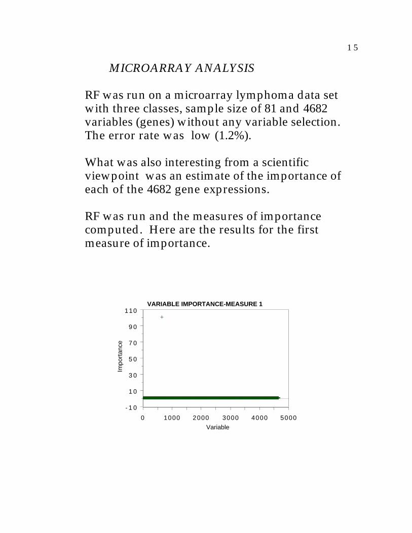
MICROARRAY ANALYSIS
RF was run on a microarray lymphoma data setwith three classes, sample size of 81 and 4682variables (genes) without any variable selection.The error rate was low (1.2%).
What was also interesting from a scientificviewpoint was an estimate of the importance ofeach of the 4682 gene expressions.
RF was run and the measures of importancecomputed. Here are the results for the firstmeasure of importance.
- 1 0
1 0
3 0
5 0
7 0
9 0
110
Impo
rtan
ce
0 1000 2000 3000 4000 5000
Variable
VARIABLE IMPORTANCE-MEASURE 1
1 6
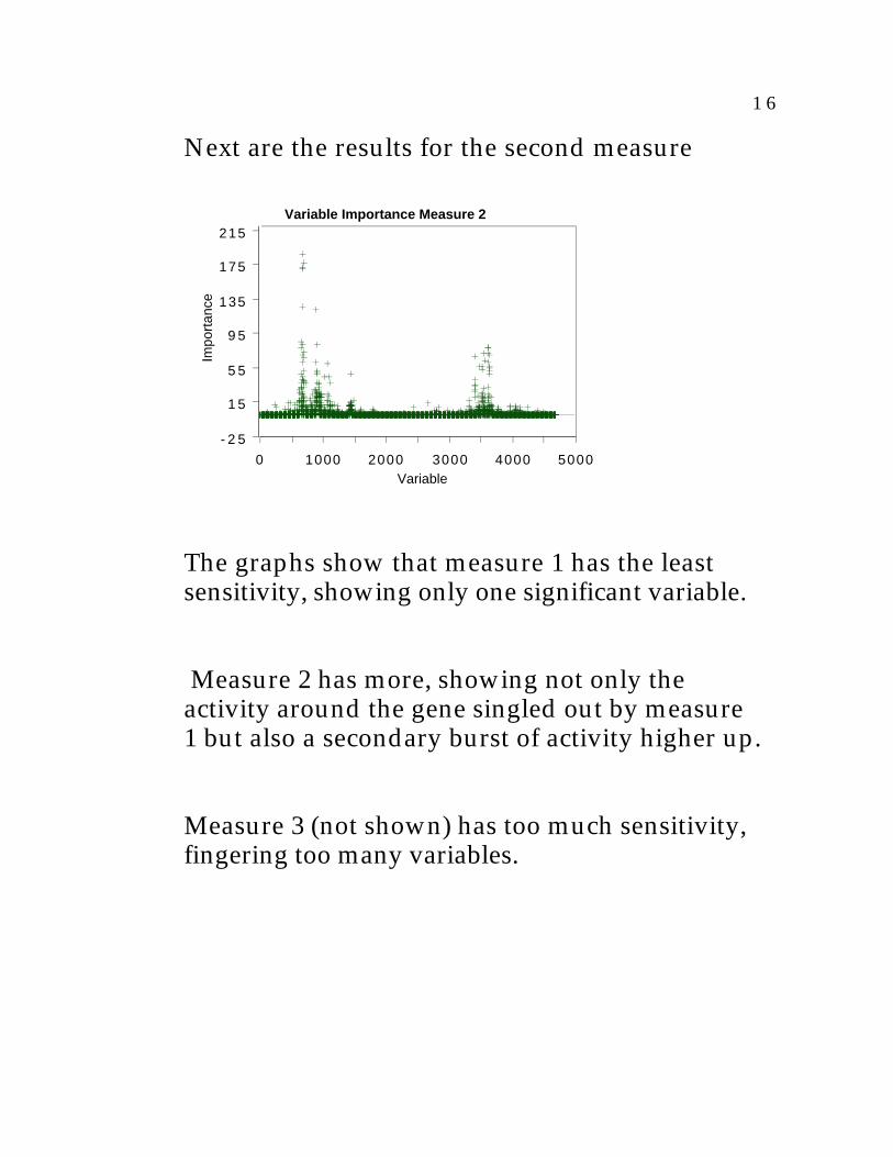
Next are the results for the second measure
- 2 5
1 5
5 5
9 5
135
175
215
Impo
rtan
ce
0 1000 2000 3000 4000 5000Variable
Variable Importance Measure 2
The graphs show that measure 1 has the leastsensitivity, showing only one significant variable.
Measure 2 has more, showing not only theactivity around the gene singled out by measure1 but also a secondary burst of activity higher up.
Measure 3 (not shown) has too much sensitivity,fingering too many variables.

1 7EFFECTS OF VARIABLES ON PREDICTIONS
Besides knowing which variables are important,another piece of information needed is how thevalues of each variable effects the prediction.
Each time case n is oob it receives a vote for aclass from its associated tree.
At the end of the run, there are available theproportions of the vote for each class and foreach case. Call these the cpv's
For each class and each variable m, compute thecpv for the jth minus the cpv with the mthvariable noised.
Plot this against the values of the mth variableand do a smoothing of the curve.
To illustrate, we use the glass data set. It's sixclass with 214 samples and nine variablesconsisting of chemical proportions.
The figure below is a plot of the decreases incpv's due to noising up the 8th variable in theglass data.
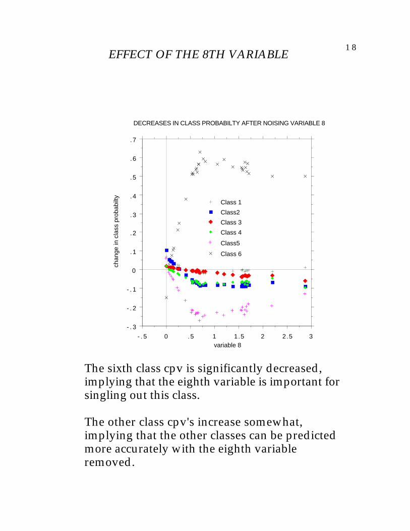
1 8EFFECT OF THE 8TH VARIABLE
- . 3
- . 2
- . 1
0
.1
.2
.3
.4
.5
.6
.7
chan
ge in
cla
ss p
roba
bilty
- . 5 0 .5 1 1.5 2 2.5 3variable 8
Class 6
Class5
Class 4
Class 3
Class2
Class 1
DECREASES IN CLASS PROBABILTY AFTER NOISING VARIABLE 8
The sixth class cpv is significantly decreased,implying that the eighth variable is important forsingling out this class.
The other class cpv's increase somewhat,implying that the other classes can be predictedmore accurately with the eighth variableremoved.

1 9
A PROXIMITY MEASURE AND CLUSTERING
Since an individual tree is unpruned, the terminalnodes will contain only a small number ofinstances.
Run all cases in the training set down the tree. Ifcase i and case j both land in the same terminalnode. increase the proximity between i and j byone.
At the end of the run, the proximities are dividedby the number of trees in the run and proximitybetween a case and itself set equal to one.
This is an intrinsic proximity measure, inherent inthe data and the RF algorithm.
To cluster-use the above proximity measures.
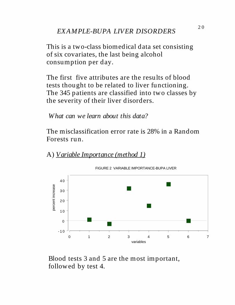
2 0 EXAMPLE-BUPA LIVER DISORDERS
This is a two-class biomedical data set consistingof six covariates, the last being alcoholconsumption per day.
The first five attributes are the results of bloodtests thought to be related to liver functioning.The 345 patients are classified into two classes bythe severity of their liver disorders.
What can we learn about this data?
The misclassification error rate is 28% in a RandomForests run.
A) Variable Importance (method 1)
- 1 0
0
1 0
2 0
3 0
4 0
perc
ent i
ncre
ase
0 1 2 3 4 5 6 7variables
FIGURE 2 VARIABLE IMPORTANCE-BUPA LIVER
Blood tests 3 and 5 are the most important, followed by test 4.

2 1
B) Clustering
Using the proximity measure outputted by RandomForests to cluster, there are two class #2 clusters.
In each of these clusters, the average of each variableis computed and plotted:
Figure 3 Cluster Variable Averages
Something interesting emerges. The class twosubjects consist of two distinct groups:
Those that have high scores on blood tests 3, 4,and 5 Those that have low scores on those tests.
We will revisit this example below.

2 2SCALING COORDINATES
The proximities between cases n and k form amatrix {prox(n,k)}. From their definition, itfollows that the values 1-prox(n,k) are squareddistances in a Euclidean space of high dimension.
Then, one can compute scaling coordinates whichproject the data onto lower dimensional spaceswhile preserving (as much as possible) thedistances between them.
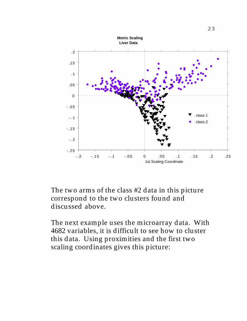
We illustrate with three examples. The first isthe graph of 2nd vs. 1st scaling coordinates forthe liver data
2 3
- . 25
- . 2
- . 15
- . 1
- . 05
0
.05
.1
.15
.2
- . 2 - . 15 - . 1 - . 05 0 .05 .1 .15 .2 .251st Scaling Coordinate
class 2
class 1
Metric Scaling Liver Data
The two arms of the class #2 data in this picturecorrespond to the two clusters found anddiscussed above.
The next example uses the microarray data. With4682 variables, it is difficult to see how to clusterthis data. Using proximities and the first twoscaling coordinates gives this picture:

2 4
- . 2
- . 1
0
.1
.2
.3
.4
.5
.62n
d S
calin
g C
oord
inat
e
- . 5 - . 4 - . 3 - . 2 - . 1 0 .1 .2 .3 .41st Scaling Coordinate
class 3
class 2
class 1
Metric ScalingMicroarray Data
Random forests misclassifies one case. This caseis represented by the isolated point in the lowerleft hand corner of the plot.
The third example is glass data with 214 cases, 9variables and 6 classes. This data set has beenextensively analyzed (see Pattern recognition andNeural Networkks-by B.D Ripley). Here is a plotof the 2nd vs. the 1st scaling coordinates.:

2 5
- . 4
- . 3
- . 2
- . 1
0
.1
.2
.3
.4
2nd
scal
ing
coor
dina
te
- . 5 - . 4 - . 3 - . 2 - . 1 0 .1 .21st scaling coordinate
class 6
class 5
class 4
class 3
class 2
class 1
Metric Scaling Glass data
None of the analyses to data have picked up thisinteresting and revealing structure of the data--compare the plots in Ripley's book.
We don't understand its implications yet.

2 6
OUTLIER LOCATION
Outliers are defined as cases having smallproximities to all other cases.
Since the data in some classes is more spread outthan others, outlyingness is defined only withrespect to other data in the same class as thegiven case.
To define a measure of outlyingness,we first compute, for a case n, the sum of thesquares of prox(n,k) for all k in the same class ascase n.
Take the inverse of this sum--it will be large if theproximities prox(n,k) from n to the other cases kin the same class are generally small.
Denote this quantity by out(n).
For all n in the same class, compute the median ofthe out(n), and then the mean absolute deviationfrom the median.
Subtract the median from each out(n) and divideby the deviation to give a normalized measure ofoutlyingness.
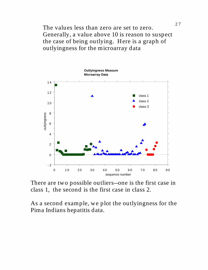
2 7The values less than zero are set to zero.Generally, a value above 10 is reason to suspectthe case of being outlying. Here is a graph ofoutlyingness for the microarray data
- 2
0
2
4
6
8
1 0
1 2
1 4
outly
ingn
ess
0 1 0 2 0 3 0 4 0 5 0 6 0 7 0 8 0 9 0sequence number
class 3
class 2
class 1
Outlyingness MeasureMicroarray Data
There are two possible outliers--one is the first case inclass 1, the second is the first case in class 2.
As a second example, we plot the outlyingness for thePima Indians hepatitis data.
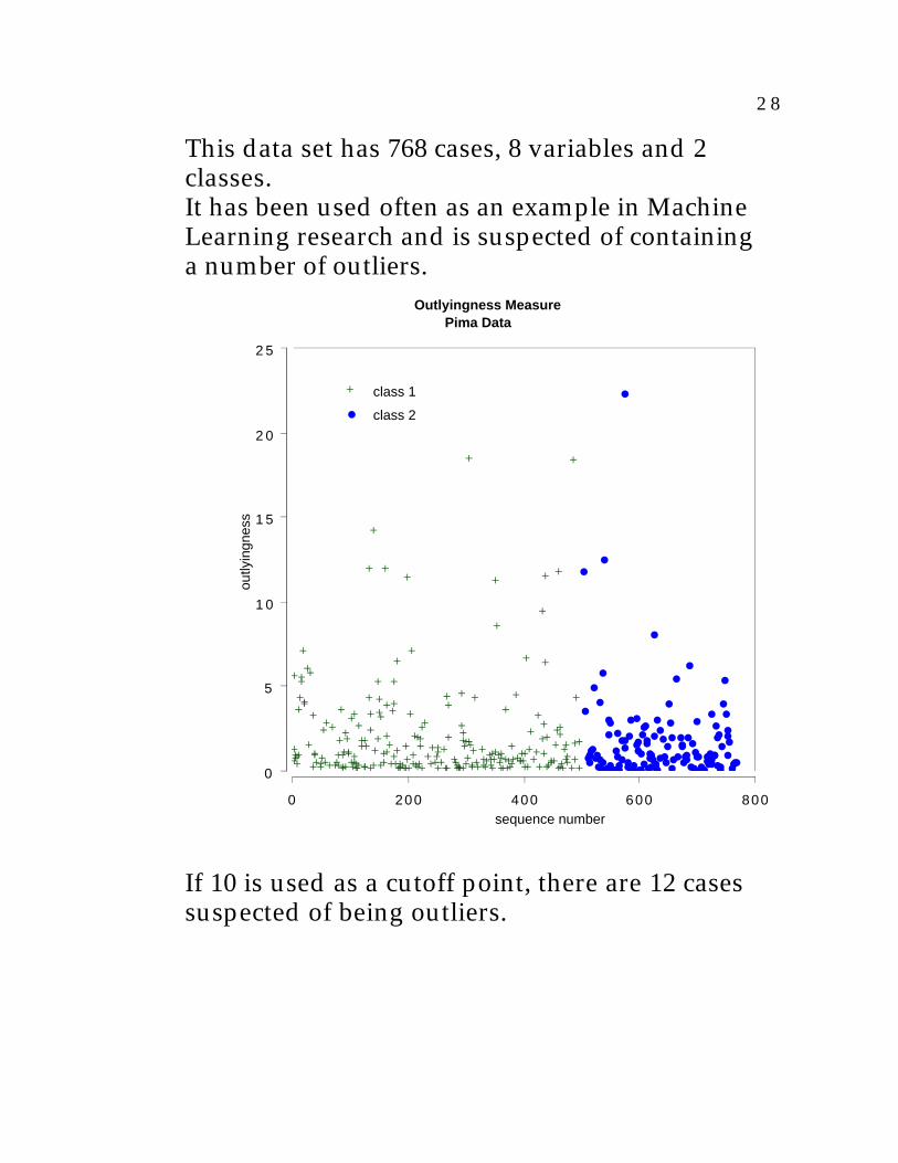
2 8
This data set has 768 cases, 8 variables and 2classes.It has been used often as an example in MachineLearning research and is suspected of containinga number of outliers.
0
5
1 0
1 5
2 0
2 5
outly
ingn
ess
0 200 400 600 800sequence number
class 2
class 1
Outlyingness Measure Pima Data
If 10 is used as a cutoff point, there are 12 cases suspected of being outliers.

2 9
ANALYZING UNLABELED DATA
Using an interesting device, it is possible to turnproblems about the structure of unlabeled data(i.e. clusters, etc.) into a classification context.
Unlabeled date consists of N vectors {x(n)} in Mdimensions. These vectors are assigned classlabel 1.
Another set of N vectors is created and assignedclass label 2.
The second synthetic set is created byindependent sampling from the one-dimensionalmarginal distributions of the original data.
For example, if the value of the mth coordinate ofthe original data for the nth case is x(m,n), then acase in the synthetic data is constructed asfollows:
Its first coordinate is sampled at random from theN values x(1,n), its second coordinate is sampledat random from the N values x(2,n), and so on.
Thus the synthetic data set can be considered tohave the distribution of M independent variableswhere the distribution of the mth variable is thesame as the univariate distribution of the mthvariable in the original data.
3 0
RUN RF
When this two class data is run through randomforests a high misclassification rate--say over 40%,implies that there is not much dependencestructure in the original data.
That is, that its structure is largely that of Mindependent variables--not a very interestingdistribution.
But if there is a strong dependence structurebetween the variables in the original data, theerror rate will be low.
n this situation, the output of random forests canbe used to learn something about the structure ofthe data.
The following is an example that comes from datasupplied by Merck.

3 1
APPLICATION TO CHEMICAL SPECTRA
Data supplied by Merck consists of the first 468spectral intensities in the spectrums of 764compounds. The challenge presented by Merckwas to find small cohesive groups of outlyingcases in this data.
Creating the 2nd synthetic class there wasexcellent separation with an error rate of 0.5%,indicating strong dependencies in the originaldata. We looked at outliers and generated thisplot.
0
1
2
3
4
5
outly
ingn
ess
0 100 200 300 400 500 600 700 800sequence numner
Outlyingness Measure Spectru Data
3 2
USING SCALING
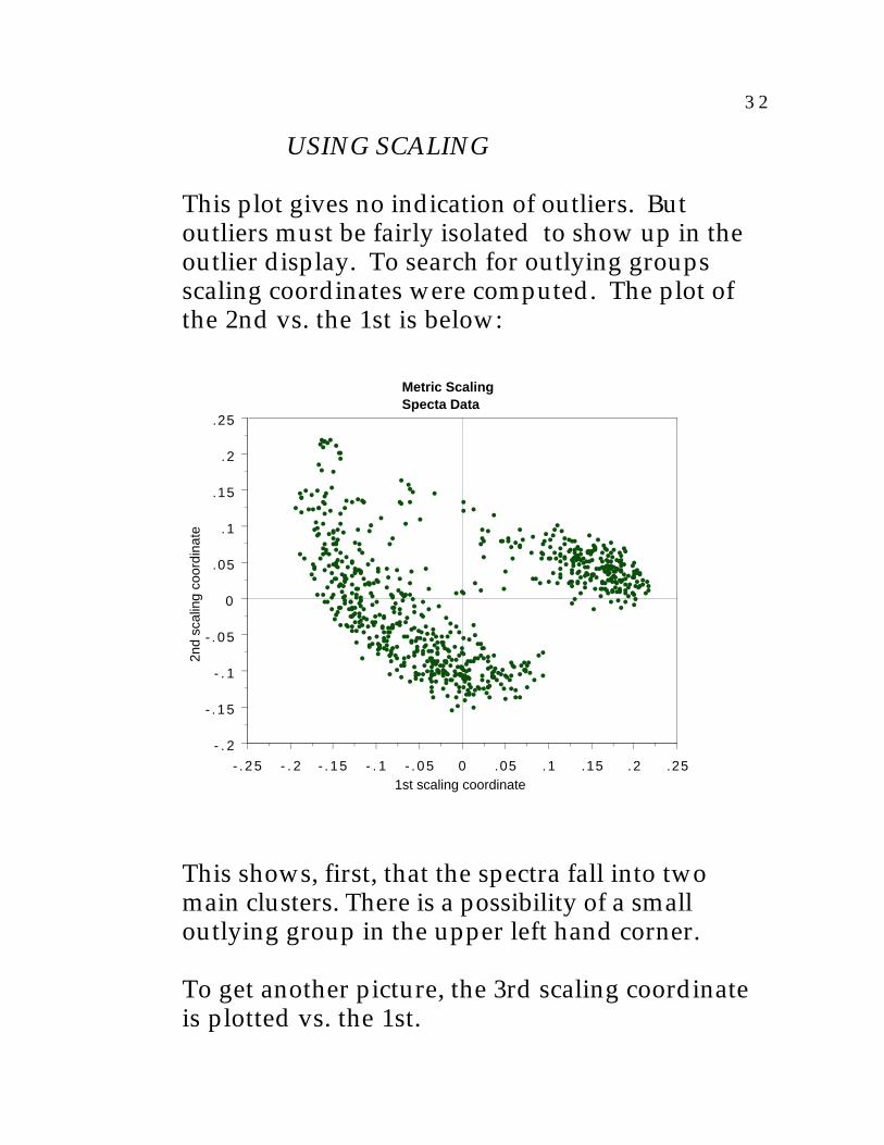
This plot gives no indication of outliers. Butoutliers must be fairly isolated to show up in theoutlier display. To search for outlying groupsscaling coordinates were computed. The plot ofthe 2nd vs. the 1st is below:
- . 2
- . 15
- . 1
- . 05
0
.05
.1
.15
.2
.25
2nd
scal
ing
coor
dina
te
- . 25 - . 2 - . 15 - . 1 - . 05 0 .05 .1 .15 .2 .251st scaling coordinate
Metric ScalingSpecta Data
This shows, first, that the spectra fall into twomain clusters. There is a possibility of a smalloutlying group in the upper left hand corner.
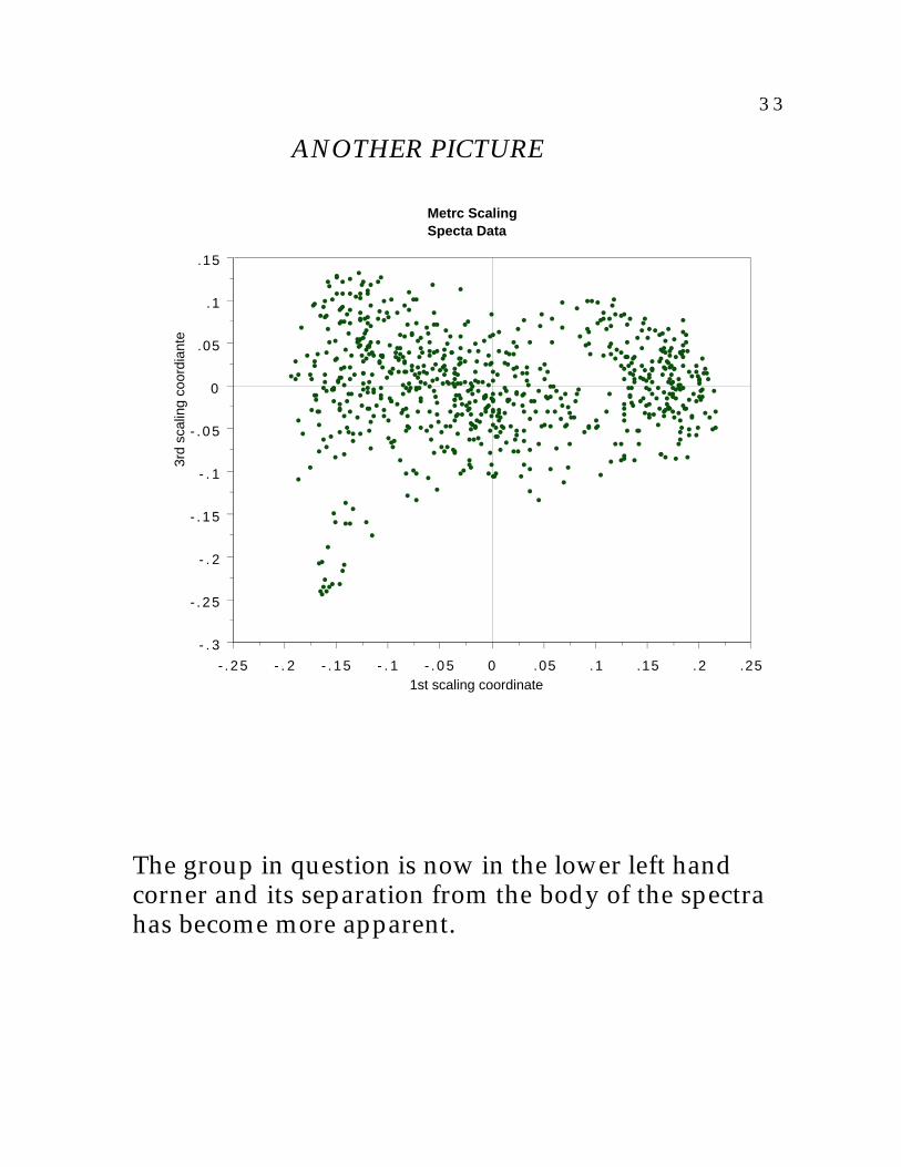
To get another picture, the 3rd scaling coordinateis plotted vs. the 1st.
3 3
ANOTHER PICTURE
- . 3
- . 25
- . 2
- . 15
- . 1
- . 05
0
.05
.1
.15
3rd
scal
ing
coor
dian
te
- . 25 - . 2 - . 15 - . 1 - . 05 0 .05 .1 .15 .2 .251st scaling coordinate
Metrc ScalingSpecta Data
The group in question is now in the lower left handcorner and its separation from the body of the spectrahas become more apparent.

3 4
TO SUMMARIZE
i ) With any model fit to data, the information extracted is about the model--not nature.
ii) The better the model emulates nature, the more reliable our information.
iii) A prime criterion as to how good the emulation is the error rate in predicting future outcomes.
iv) The most accurate current prediction algorithms can be applied to very high dimensional data, but are also complex.
v) But a complex predictor can yield a wealthof "interpretable" scientific information aboutthe prediction mechanism and the data.
CURTAIN!
Curtain Call:
Random Forests is free software.
www.stat.berkeley,edu/users/breiman

3 5