WASHINGTON UNIVERSITY - CREL Homecrelonweb.eec.wustl.edu/theses/mohan/thesis3.doc · Web...

WASHINGTON UNIVERSITY

SEVER INSTITUTE OF TECHNOLOGY

DEPARTMENT OF CHEMICAL ENGINEERING

______________________________________________________________

PERFORMANCE STUDIES OF TRICKLE BED REACTORS

by

Mohan R. Khadilkar

Prepared under the direction of Prof. M. P. Dudukovic and Prof. M. H. Al-Dahhan

___________________________________________________________________

A dissertation presented to the Sever Institute of

Washington University in partial fulfillment

of the requirements for the degree of

DOCTOR OF SCIENCE

August, 1998

Saint Louis, Missouri, USA

WASHINGTON UNIVERSITY

SEVER INSTITUTE OF TECHNOLOGY

DEPARTMENT OF CHEMICAL ENGINEERING____________________________________________________

ABSTRACT

_____________________________________________________________________

PERFORMANCE STUDIES OF TRICKLE BED REACTORS

by Mohan R. Khadilkar

__________________________________________________________

ADVISORS: Prof. M. P. Dudukovic and Prof. M. H. Al-Dahhan

___________________________________________________

August, 1998

Saint Louis, Missouri, USA

_______________________________________

A thorough understanding of the interaction between kinetics, transport, and

hydrodynamics in trickle bed reactors under different reaction and operating conditions is

necessary to design, scale-up, and operate them in such a way as to achieve the best

performance. In this study, systematic experimental and theoretical investigations have

been carried out to study trickle bed performance in different modes of operation and

reaction conditions in order to improve our understanding of the factors governing scale-

up and performance.

The first part of this study is focused on comparison of performance of down-

flow (trickle bed reactors-TBR) and up-flow reactors (packed bubble columns-PBC)

without and with fines to assess their applicability as test reactors for scale-up and scale-

down studies for different reaction systems (gas and liquid reactant limited). This has

been accomplished by experimentation on hydrogenation of a-methylstyrene to cumene

in hexane solvent over 2.5% Pd on alumina extrudate catalyst as a test reaction, and, by

comparing the predictions of existing models for both modes of operation with each

other and with the data. Comparison of results obtained at different pressures, liquid

reactant feed concentrations, and gas flow rates has been presented, and differences in

performance of the two reactor modes of operation explained on the basis of the observed

shift from gas limitation to liquid limitation. Experiments in the bed diluted with fines

have been conducted to demonstrate the fact that hydrodynamics and kinetics can be de-

coupled by using fines. It has also been shown that the advantage of upflow or downflow

mode of operation depends on whether liquid or gas reactant is rate limiting, and that an

approximate criterion for identifying the limiting reactant can explain most of the data

reported in the literature on these two modes of operation. Comparison of experimental

observations and predictions of the reactor scale and pellet scale models available in the

literature is also reported. A rigorous steady state model for the solution of the reactor

and pellet scale flow-reaction-transport phenomena based on multicomponent transport is

proposed to overcome assumptions in earlier models such as non-volatile reactants, dilute

solutions, isothermal, isobaric operation, and constant phase velocities. Predictions of

this model are compared against data available in literature for a system with volatile

liquids.

The second part of this study is devoted to investigating the performance of

trickle bed reactors under unsteady state liquid flow modulation (periodic operation) for

gas and liquid limited reactions. Exploitation of the opportunity of alternately and

systematically supplying the liquid and gaseous reactants to the catalyst during and after

the liquid pulse, respectively, has been shown to result in performance different from that

obtained under steady state conditions. The effect of key parameters such as extent of

gas/liquid limitation, total cycle period, cycle split, liquid mass velocity, and liquid solid

contacting have been investigated experimentally to demonstrate the cause-effect

relationships in unsteady state operation. Performance enhancement has been

demonstrated to be dependent on cycling parameters such as cycle period, split and

iii

induced flow modulation frequency for gas limited conditions. It has been observed to be

strongly dependent on extent of catalyst wetting under liquid limited conditions.

Rigorous modeling of the interphase transport of mass and energy based on the Maxwell-

Stefan approach at the reactor and catalyst level has been used to simulate the processes

occurring under unsteady state conditions for a general multi-component system. Reactor

performance results for several flow modulation simulation tests for a hydrogenation

reaction have been presented and discussed.

iv

ContentsPage

List Of Tables...................................................................................................... ix

List Of Illustrations............................................................................................... x

Acknowledgements............................................................................................ xiv

Nomenclature.................................................................................................... xvi

Chapter 1. Introduction......................................................................................... 1

1.1 Motivation........................................................................................... 4

1.1.1 Comparison of Down-flow (Trickle Bed Reactor-TBR) and

Up-flow (Packed Bubble Column-PBC) Reactors........................4

1.1.2 Unsteady State Operation of Trickle Bed Reactors...............7

1.2 Objectives.........................................................................................12

1.2.1 Comparison of Down-flow (TBR) and Up-flow (PBC)

Performance................................................................................12

1.2.2 Unsteady State Operation of Trickle Bed Reactors.............13

Chapter 2. Background.......................................................................................15

2.1 Laboratory Reactors – Performance Comparison and Scaleup Issues 15

2.1.1 Literature on Performance Comparison..............................15

2.1.2 Criterion for Gas and Liquid Reactant Limitation...............16

2.2 Literature on Unsteady State Operation of Trickle Bed Reactors.......20

2.2.1 Strategies for Unsteady State Operation..............................21

2.3 Review of Models for TBR Performance..........................................27

2.3.1 Steady State Models............................................................27

2.3.2 Unsteady State Models for Trickle Bed Reactors................28

2.4 Modeling Multicomponent Effects....................................................35

2.5 Balance Relations for Multiphase Systems........................................39

v

Chapter 3. Experimental Facility........................................................................42

3.1 High Pressure Trickle Bed Setup.......................................................42

3.1.1 Reactor and Distributors for Upflow and Downflow...........42

3.1.2 Gas-Liquid Separator and Level Control.............................43

3.1.4 Liquid and Gas Delivery System........................................44

3.1.5 Data Acquisition and Analysis............................................49

3.2 Operating Procedures and Conditions................................................50

3.2.1 Steady State TBR-PBC Comparison Experiments..............50

3.2.2 Bed Dilution and Experiments with Fines...........................52

3.2.3 Unsteady State Experiments...............................................54

Chapter 4. Experimental Results.........................................................................57

4.1 Steady State Experiments on Trickle Bed Reactor and Packed Bubble

Column................................................................................................... 57

4.1.1 Effect of Reactant Limitation on Comparative Performance

of TBR and PBC..........................................................................57

4.1.2 Effect of Reactor Pressure on Individual Mode of Operation61

4.1.3 Effect of Feed Concentration of a-methylstyrene on

Individual Mode of Operation.....................................................62

4.1.5 Effect of Gas Velocity and Liquid-Solid Contacting

Efficiency....................................................................................67

4.2 Comparison of Down-flow (TBR) and Up-flow (PBC) Reactors with

Fines....................................................................................................... 69

4.2.1 Effect of Pressure in Diluted Bed on Individual Mode of

Operation..................................................................................... 72

4.2.2 Effect of Feed Concentration in Diluted Bed on Individual

Mode of Operation......................................................................72

vi

4.3 Unsteady State Experiments in TBR.................................................74

4.3.1 Performance Comparison for Liquid Flow Modulation under

Gas and Liquid Limited Conditions.............................................74

4.3.2 Effect of Modulation Parameters (Cycle Period and Cycle

Split) on Unsteady State TBR Performance.................................77

4.3.3 Effect of Amplitude (Liquid Mass Velocity) on Unsteady

State TBR Performance...............................................................80

4.3.4 Effect of Liquid Reactant Concentration and Pressure on

Performance................................................................................82

4.3.5 Effect of Cycling Frequency on Unsteady State Performance85

4.3.6 Effect of Base-Peak Flow Modulation on Performance.......88

Chapter 5. Modeling Of Trickle Bed Reactors....................................................90

5.1 Evaluation of Steady State Models for TBR and PBC.......................90

5.1.1 Reactor Scale Model (El-Hisnawi et al., 1982)...................90

5.1.2 Pellet Scale Model (Beaudry et al., 1987)...........................92

5.2 Unsteady State Model for Performance of Trickle Bed Reactors in

Periodic Operation................................................................................102

5.2.1 Reactor Scale Transport Model and Simulation................105

5.2.2 Flow Model Equations......................................................110

5.2.3 Multicomponent Transport at the Interface.......................116

5.2.4 Catalyst Level Rigorous and Apparent Rate Solution........120

Chapter 6. Conclusions.....................................................................................138

6.1 Recommendations for Future Work.................................................140

Appendix A. Slurry Experiments: Intrinsic Rate At High Pressure..................143

Appendix B. Correlations Used In Model Evaluation.......................................146

Appendix C. Flow Charts For The Unsteady State Simulation Algorithm.........147

vii

Appendix D Maxwell-Stefan Equations For Multicomponent Transport...........150

Appendix E Evaluation Of Parameters For Unsteady State Model....................155

Appendix F. Experimental Data From Steady And Unsteady Experiments.......158

Appendix G. Simulation of Flow using CFDLIB..............................................177

Appendix H. Improved Prediction of Pressure Drop in High Pressure Trickle Bed

Reactors............................................................................................................ 188

References........................................................................................................ 196

VITA................................................................................................................ 201

viii

List Of TablesTable Page

Table 2. 1 Identification of the Limiting Reactant for Literature and Present Data..Error!

Bookmark not defined.

Table 2. 2 Literature Studies on Unsteady State Operation in Trickle Beds....................24

Table 2. 3 Review of Recent Steady State Reaction Models for Trickle Bed Reactors. . .30

Table 2. 4 Review of Unsteady State Models for Trickle Bed Reactors..........................33

Table 3. 1 Catalyst and Reactor Properties for Steady State Experiments.......................53

Table 3. 2 Range of Operating Conditions for Steady State Experiments.......................53

Table 3. 3 Catalyst and Reactor Properties for Unsteady State Conditions.....................56

Table 3. 4 Reaction and Operating Conditions for Unsteady State Experiments.............56

Table 5. 1 Governing Equations for El-Hisnawi (1982) Model......................................96

Table 5. 2 Governing Equations for Beaudry (1987) Model...........................................97

Table 5. 3 Typical Equation Vector for the Stefan-Maxwell Solution of Gas-Liquid

Interface............................................................................................................... 119

Table 5. 4 Typical Stefan Maxwell Equation Vector for a Half Wetted Pellet..............122

Table 5. 5 Energy Flux Equations for Gas-Liquid, Liquid-Solid, and Gas-Solid Interfaces

............................................................................................................................. 124

Table 5. 6 Equation Set for Single Pellet Model...........................................................126

Table 5. 7 Catalyst Level Equations for Rigorous Three Pellet Model..........................128

Table 5. 8 List of Model Variables and Equations........................................................129

Table A. 1 Rate Constants Obtained from Slurry Data at Different Pressures...............144

ix

List Of FiguresFigure Page

Figure 1. 1 Trickle bed Reactor: Flow Regimes and Catalyst Wetting Conditions............3

Figure 2. 1 Time Averaged SO2 Oxidation Rates of Haure et al. (1990)........................26

Figure 2. 2 Experimental and Predicted Temperature Profiles of Haure et al. (1990)....26

Figure 2. 3 Enhancement in Periodic Operation Observed by Lange et al. (1993)..........26

Figure 3. 1 Reactor and Gas-Liquid Separator................................................................46

Figure 3. 2 Down-flow and Up-flow Distributor for TBR and PBC Operation...............47

Figure 3. 3 Experimental Setup for Unsteady State Flow Modulation Experiments........48

Figure 3. 4 Data Acquisition System..............................................................................49

Figure 3. 5 Basket Reactor Catalyst Stability Test for Palladium on Alumina Catalyst..50

Figure 4. 1 Trickle Bed and Up-flow Performance at CBi=7.8%(v/v) and Ug =4.4 cm/s at

30 psig.................................................................................................................... 60

Figure 4. 2 Comparison of Down-flow and Up-flow Performance at CBi=3.1%(v/v) at

200 psig.................................................................................................................. 60

Figure 4. 3 Effect of Pressure at Low a-methylstyrene Feed Concentration on Upflow

Reactor Performance.............................................................................................. 63

Figure 4. 4 Effect of Pressure at Low a-methylstyrene Feed Concentration (3.1% v/v) on

Downflow Performance.......................................................................................... 63

Figure 4. 5 Effect of Pressure at Higher a-methylstyrene Feed Concentration on

Downflow Performance.......................................................................................... 64

x

Figure 4. 6 Effect of a-methylstyrene Feed Concentration at 100 psig on Upflow

Performance........................................................................................................... 65

Figure 4. 7 Effect of a-methylstyrene Feed Concentration at 100 psig on Downflow

Performance........................................................................................................... 65

Figure 4. 8 Effect of a-methylstyrene Feed Concentration at 200 psig on Downflow

Performance........................................................................................................... 66

Figure 4. 9 Effect of a-methylstyrene Feed Concentration at 200 psig on Upflow

Performance........................................................................................................... 66

xi

Figure 4. 10 Effect of Gas Velocity on Reactor Performance at 100 psig......................68

Figure 4. 11 Pressure Drop in Downflow and Upflow Reactors and Contacting Efficiency

for Downflow Reactor at 30 and 200 psig..............................................................68

Figure 4. 12 Effect of Fines on Low Pressure Down-flow Versus Up-flow Performance

............................................................................................................................... 71

Figure 4. 13 Effect of Fines on High Pressure Down-flow Versus Up-flow Performance

............................................................................................................................... 71

Figure 4. 14 Effect of a-methylstyrene Feed Concentration at Different Pressures on

Performance of Downflow with Fines....................................................................73

Figure 4. 15 Effect of a-methylstyrene Feed Concentration at Different Pressures on

Performance of Upflow with Fines.........................................................................73

Figure 4. 16 Comparison of Steady and Unsteady State Performance under Liquid

Limited Conditions ( < 4).....................................................................................76

Figure 4. 17 Comparison of Steady and Unsteady State Performance under Gas Limited

Conditions ( ~25).................................................................................................76

Figure 4. 18 Effect of Cycle Split () on Unsteady State Performance under Gas Limited

Conditions.............................................................................................................. 79

Figure 4. 19 Effect of Total Cycle Period () on Unsteady State Performance under Gas

Limited Conditions................................................................................................. 79

Figure 4. 20 Effect of Liquid Mass Velocity on Unsteady State Performance under Gas


Figure 4. 21 Effect of Liquid Reactant Feed Concentration on Unsteady State

Performance under Gas Limited Conditions...........................................................84

Figure 4. 22 Effect of Operating Pressure on Unsteady State Performance under Gas


xii

Figure 4. 23 Effect of Cycling Frequency on Unsteady State Performance under Gas


Figure 4. 24 Effect of Cycling Frequency on Unsteady State Performance....................87

Figure 4. 25 Unsteady State Performance with BASE-PEAK Flow Modulation under

Liquid Limited Conditions.....................................................................................89

Figure 4. 26 Effect of Liquid Mass Velocity on Steady State Liquid-Solid Contacting

Efficiency............................................................................................................... 89

Figure 5. 1 Upflow and Downflow Performance at Low Pressure (gas limited condition):

Experimental data and model predictions...............................................................99

Figure 5. 2 Upflow and Downflow Performance at High Pressure (liquid limited

condition): Experimental data and model predictions.............................................99

Figure 5. 3 Effect of Feed Concentration on Downflow Performance..........................100

Figure 5. 4 Effect of Feed Concentration on Predicted Upflow Performance...............100

Figure 5. 5 Estimates of volumetric mass transfer coefficients in the range of operation

from published correlations (G-L (downflow) Fukushima and Kusaka (1977), L-S

(downflow) Tan and Smith (1980), G-L (upflow) Reiss (1967), L-S (upflow)

Spechhia (1978)).................................................................................................. 101

Figure 5. 6 Phenomena Occurring in Trickle Bed under Periodic Operation................103

Figure 5. 7 Representation of the Catalyst Level Solution...........................................127

Figure 5. 8: Transient Alpha-methylstyrene (a-MS) Concentration Profiles at Different

Axial Locations.................................................................................................... 132

Figure 5. 9 Transient Alpha-methylstyrene Concentration Profile Development with

Time (shown in seconds in the legend table)........................................................132

Figure 5. 10 Axial Profiles of Cumene Concentration at Different Simulation Times

(shown in seconds in the legend table)..................................................................133

xiii

Figure 5. 11 Transient Hydrogen Concentration Profiles at Different Axial Locations.133

Figure 5. 12 Transient Liquid Holdup Profiles at Different Axial Locations in Periodic

Flow..................................................................................................................... 134

Figure 5. 13 Transient Liquid Velocity Profiles at Different Axial Locations in Periodic

Flow..................................................................................................................... 135

Figure 5. 14 Cumene Concentration Profiles during Periodic Flow Modulation...........136

Figure 5. 15 Intra-catalyst Hydrogen Concentration Profiles during Flow Modulation for

a Previously Externally Wetted Catalyst Pellet at Different Axial Locations........137

Figure 5. 16 Intra-Catalyst Alpha-methylstyrene Concentration Profiles during Flow

Modulation for a Previously Externally Dry Catalyst Pellet at Different Axial

Locations.............................................................................................................. 137

Figure A. 1 Slurry conversion versus time at different pressures..................................145

Figure A. 2 Comparison of the Model Fitted Alpha-methylstyrene concentrations to

experimental values..............................................................................................145

xiv

AcknowledgementsI wish to express my heartfelt gratitude to my advisor Professor Dudukovic for

the opportunity to undertake this work under his supervision. His advice, encouragement

of independent thought, and patience was indeed invaluable in making this work

possible. I would also like to thank my co-advisor Prof. Al-Dahhan, whose advice and

interest in experimental aspects of the project made it possible for me to overcome many

obstacles. I would like to acknowledge the members of my committee, namely, Prof.

Babu Joseph, Prof. R.Gardner, Dr. Manuk Colakyan of Union Carbide Corporation, and

Dr. Ramesh Gupta of Exxon Research and Engineering for taking interest in my work

and examining my thesis and providing useful comments and suggestions.

I wish to acknowledge the financial support of the Industrial Participants of the

CREL consortium, which made the research possible. In particular, I would like to thank

Dr. Colakyan of Union Carbide Corporation for allowing me to gain practical experience

related to the first part of this thesis by participating and reviewing my work on many

aspects of this project. I am also grateful to Dr. Ramesh Gupta for his ideas and insights

into the implementation of the second part of this work. Acknowledgements are also due

to the Agricultural Group at Monsanto Company, particularly Dr. R. Kahney, Dr. S.

Chou, and G. Ahmed for their project on complex reaction networks, experience form

which was helpful in several aspects of this work. I would also like to thank Dr. Patrick

Mills of DuPont Central Research for his advice and help with model development on

systems with volatiles.

Several people at CREL and in the Chemical Engineering Department have made

significant contributions in make my work and life at Washington University. In

particular, I would like to thank Mr. Yuanxin Wu and Mr. Yi Jiang for their help and

xv

support in the experimental work on several projects undertaken in the trickle bed reactor

laboratory. My sincere acknowledgements also go to Steve Picker and John Krietler for

their help in modifying and maintaining the high pressure trickle bed facility in good

shape throughout the projects involved. My sincere gratitude to Dr. S. Kumar and Dr. Y.

Yamashita for their help in resolving numerous computational aspects of the projects. My

sincere acknowledgements also go to Dr. M. Kulkarni, Dr. S. Karur, and Dr. S.

Degaleesan whose help and encouragement was invaluable throughout my stay at

Washington University.

I sincerely acknowledge the help and assistance offered by all the past and present

members of CREL including Zhen Xu, P. Gupta, S. Roy, Alain Chone, Dr. J. Chen, Dr.

Y. Pan, Marco Roveda and many others. I also wish to thank the entire Chemical

Engineering Department, particularly the secretaries for their help with numerous

formalities. Finally, thanks to my roommates and friends whose company made my stay

in St. Louis a pleasant and memorable one.

Last, but not the least, my heartfelt gratitude goes to my parents and my sister for

their patience and support and their sustained belief in my abilities which help me get

through the vicissitudes of student life.

Mohan R. Khadilkar

Washington University, St. Louis

August, 1998

xvi

NomenclatureaGS gas-solid interfacial area (m2/m3).

aGL gas-solid interfacial area (m2/m3).

a'GL gas-Liquid total interfacial area (m2/m3).

aLS liquid-solid interfacial area (m2/m3).

ct molar density (mol/m3)

C(AMS) alpha-methylstyrene concentration

C*(H2) saturation concentration of hydrogen

CA* concentration of gaseous reactant in liquid phase (mol/m3)

CBi concentration of liquid reactant in liquid phase (mol/m3)

CiL liquid phase concentration of species i (mol/m3).

CiCP concentration of species i in the catalyst (mol/m3).

CiG gas phase concentration of species i (mol/m3).

CPmixG gas phase specific heat (J/kg K).

CPmixL liquid phase specific heat (J/kg K).

De effective diffusivity (m2/s)

DeA effective diffusivity of gaseous reactant in the catalyst (m2/s)

DeB effective diffusivity of liquid reactant in the catalyst (m2/s)

Dei effective diffusivity of reactant i in the catalyst (m2/s)

EV energy transfer flux from bulk gas to gas-liquid interface (J/ m2s).

EL energy transfer flux from gas-liquid interface to liquid (J/ m2s).

ES energy transfer flux from solid to liquid-solid interface (J/ m2s).

ELS energy transfer flux from liquid-solid interface to liquid (J/ m2s).

g gravitational acceleration (m/s2).

GaL liquid phase Galileo number.

xvii

GaG gas phase Galileo number.

HiV partial molar enthalpy of component i in vapor phase (J/mol).

HiL partial molar enthalpy of component i in liquid phase (J/mol).

HiS partial molar enthalpy of component i in liquid phase (J/mol).

hL gas-liquid interface to liquid heat transfer coefficient (J/ m2 s K).

hLS solid-liquid interface to liquid heat transfer coefficient (J/ m2 s K).

hS solid-liquid interface to solid heat transfer coefficient (J/ m2 s K).

hV gas-liquid interface to gas heat transfer coefficient (J/ m2 s K).

J molar diffusion flux relative to average velocity (mol/m2s).

(ka)GL volumetric gas-liquid mass transfer coefficient ( 1/s)

kLS.aLS volumetric liquid-solid mass transfer coefficient (1/s)

[kLik] liquid side mass transfer coefficient (m/s).

[kVik] liquid side mass transfer coefficient (m/s).

ke effective thermal conductivity of catalyst (J/m s K).

K interphase momentum transfer coefficient (kg/m3).

L mass velocity of liquid (kg/m2s)

L half the length of characteristic pellet (m).

Mi molecular weight of species i (kg/kgmole).

NiV flux of component i (vapor to gas-liquid interface) (mol/m2s).

NiL flux of component i (gas-liquid interface to liquid) (mol/m2s).

NiLS flux of component i (liquid to liquid-solid interface) (mol/m2s).

NiS flux of component i (liquid-solid interface to solid) (mol/m2s).

P operating pressure (psig)

P pressure (N/m2).

DP pressure drop (N/m2).

QL, QG volumetric flow rate of liquid, gas

q heat flux (J/m2s)

xviii

RW reaction rate on fully wetted catalyst pellet (mol/m3s).

RDW reaction rate on half wetted catalyst pellet (mol/m3s).

RD reaction rate on fully externally dry catalyst pellet (mol/m3s).

ROV overall reaction rate (mol/m3s).

ReL liquid phase Reynolds number.

ReG gas phase Reynolds number.

(rA)obs observed rate of reaction (mol/m3s)

Sx catalyst external surface area (m2)

TCP catalyst temperature (K)

TG gas temperature (K)

TA ambient temperature (K)

TL liquid temperature (K)

TI gas-liquid interface temperature (K).

TILS liquid-Solid interface temperature (K).

UIL liquid interstitial (actual) velocity (m/s).

UIG gas interstitial (actual) velocity (m/s).

Ug gas velocity (m/s)

VL, VG superficial velocity of liquid, gas

VR reactor volume, (m3)

Vp catalyst Pellet Volume ( m3)

X(ss) steady state conversion

X(us) unsteady state conversion

x mole fraction in the liquid phase.

x' spatial coordinate in catalyst pellet (m).

y mole fraction in the gas phase.

z axial coordinate (m).

Greek Symbols

xix

reactant limitation criterion (=De (AMS) C(AMS) feed/ De (H2) C*(H2))

total cycle period, s

cycle split

flow modulation frequency, Hz

b bootstrap matrix in Maxwell-Stefan formulation

a',b' order of reaction with respect to species i and j.

e,eB bed voidage.

eG gas holdup.

eP porosity.

eL liquid holdup.

esL static holdup of liquid.

ni stoichiometric coefficient of component i

rL liquid phase density (kg/m3).

rG gas phase density (kg/m3).

hCE contacting efficiency.

yL dimensionless liquid phase drag.

yG dimensionless gas phase drag.

li difference in component molar enthalpies (J/mol).

axial coordinate (m).

temporal coordinate (s).

NOTATION

aGS Gas-solid interfacial area (m2/m3)

aGL Gas-solid interfacial area (m2/m3)

aLS Liquid-solid interfacial area (m2/m3)

xx

B Mass transfer coefficient matrix

ct Molar density (mol/m3)

CiL Liquid phase concentration of species i (mol /m3)

CCiL Liquid phase concentration of species i (mol /m3)

CiG Gas phase concentration of species i (mol/m3)

CCiG Gas phase concentration of species i (mol/m3)

Ct Gas phase concentration of species i (mol/m3)

De Effective diffusivity of gaseous reactant in the catalyst (m2/s)

dt Reactor diameter, m

EGL Energy transfer flux from gas to liquid phase (J/ m2s)

ELS Energy transfer flux from liquid to solid phase (J/ m2s)

EGS Energy transfer flux from gas to solid phase (J/ m2s)

ELA Energy transfer flux to ambient (J/ m2s)

fw Fractional wetting

Fd,liq Liquid-solid drag

xxi

Fd,gas Gas-solid drag

FL Liquid molar flow, mol/s

FV Liquid molar flow, mol/s

FA0 Molar flow of component A, mol/s

FB0 Molar flow of component A, mol/s

FC0 Molar flow of component A, mol/s

g Gravitational acceleration (m/s2)

HG Enthalpy of component i in vapor phase (J/kg)

HL Enthalpy of component i in liquid phase (J/kg)

hL Gas-liquid interface to liquid heat transfer coefficient (J/ m2 s K)

hLS Solid-liquid interface to liquid heat transfer coefficient (J/ m2 s K)

hGS Solid-liquid interface to solid heat transfer coefficient (J/ m2 s K)

hG Gas-liquid interface to gas heat transfer coefficient (J/ m2 s K)

h Henry’s constant

[kikL] Liquid side mass transfer coefficient (m/s)

[kikV] Liquid side mass transfer coefficient (m/s)

ke Effective thermal conductivity of catalyst (J/m s K)

k Rate constant in level I model

kW Wet pellet rate constant (1/s)

kD Dry pellet rate constant (1/s)

K Equilibrium constant

xxii

KGL Interphase momentum transfer coefficient (kg/m3s)

L Length of reactor (m)

LC Length of catalyst pellet (m)

Mi Molecular weight of species i (kg/kgmole)

N Hydrogen to cyclohexene molar feed ratio

NiGL Flux of component i (vapor to gas-liquid interface) (mol/m2s)

NCiL Intracatalyst liquid phase flux of component i (mol/m2s)

NCiG Intracatalyst gas phase flux of component i (mol/m2s)

NiLS Flux of component i (liquid to liquid-solid interface) (mol/m2s)

NiGS Flux of component i (gas to gas-solid interface) (mol/m2s)

P Pressure (N/m2)

q Heat flux (J/m2s)

R Universal gas constant (m3 atm/mol K)

RW Reaction rate on fully wetted catalyst pellet (mol/m3s)

Ri,Liq Intrinsic reaction rate in liquid filled catalyst pellet (=kWCCH2,L (mol/m3s))

RD Reaction rate on fully externally dry catalyst pellet (mol/m3s)

Ri,Gas Intrinsic reaction rate in gas filled catalyst pellet (=kDCCCyc-ene,G (mol/m3s))

Sx Catalyst external surface area (m2)

T Mixture temperature

To Inlet fluid temperature (K)

TW Wall temperature (K)

TG Gas temperature (K)

TA Ambient temperature (K)

xxiii

TL Liquid temperature (K)

TI Gas-liquid interface temperature (K)

T Liquid-solid interface temperature (K)

U Reactor to wall heat transfer coefficient

uIL Liquid interstitial (actual) velocity (m/s)

uIG Gas interstitial (actual) velocity (m/s)

uIIL Liquid interfacial velocity (m/s)

uIIG Gas interfacial velocity (m/s)

x Mole fraction in the liquid phase

Intra-pellet spatial coordinate, m

xIi Liquid phase mole fraction at the gas-liquid or liquid-solid interface for

component i

yIi Gas phase mole fraction at the gas-liquid or gas-solid interface for component i

y Mole fraction in the gas phase

z Axial coordinate (m)

Greek Symbols

a Conversion (based on cyclohexene)

b Bootstrap matrix in Maxwell-Stefan formulation

Activity correlation matrix

Intracatalyst gas-liquid interface location

e, eB Bed voidage

xxiv

eG Gas holdup

eP Porosity

eL Liquid holdup

ni Stoichiometric coefficient of component i

rL Liquid phase density (kg/m3)

rLi Liquid component mass density (kg/m3)

rG Gas phase density (kg/m3)

hCE Contacting efficiency

l Reactor effective thermal conductivity (J/m s K)

lx Latent heat (J/mol)

xxv

1

Chapter 1. Introduction

Trickle bed reactors are packed beds of catalyst with cocurrent down-flow of gas

and liquid, and are widely used in hydrocracking, hydrodesulfurization, etc., in the

petroleum industry, as well as in some selected chemical industry applications for

hydrogenation, oxidation, and chlorination and more recently in the waste treatment and

biochemical processing industry. In fact, tonnage wise, trickle beds are the most used

reactors in the entire chemical and related industries (1.6 billion metric tons annual

processing capacity (Al-Dahhan et al. (1997)), with an enormous capital invested in

design, set-up and operation of this type of reactors. Trickle bed reactors are generally

operated at high pressure (up to 30 MPa) and temperature (up to 300 o C) in the low

interaction or trickle flow regime i.e., the flowing gas is the continuous phase and liquid

flows as rivulets and films over the catalyst particles (Figure 1.1). The packing, which

occupies 55 - 65 % of the bed volume, is usually a supported catalyst in the form of

different shapes (spheres, extrudates, trilobes etc.) and sizes ranging from 1 to 3 mm.

Due to large throughputs, reactor volumes can be as high as 200 m3 with bed heights up

to 20 m in some cases. Trickle bed reactors have several advantages over other type of

multiphase reactors such as: plug flow like flow pattern, high catalyst loading per unit

volume of liquid, low power requirements, low energy dissipation, and greater flexibility

with respect to production rates and operating conditions used. Some disadvantages of

trickle bed reactors are their lower catalyst effectiveness factors due to large particle

sizes, higher pressure drops, limited use in viscous or foaming liquids, sensitivity to

thermal effects and inefficient heat removal. Despite the fact that the advantages

2

outweigh the disadvantages, trickle bed reactors have not found applications to their

fullest potential due to difficulties associated with their design and uncertainty in the

scale-up strategies used for their commercial application. These difficulties are

introduced by the complexities of two phase flow, flow distribution, and incomplete

catalyst wetting, which are not duplicated in laboratory scale experiments to the same

extent (Saroha and Nigam, 1996). In order to expand the horizon of applications of these

reactors, it is necessary to understand all the relevant complex phenomena, on the macro,

meso and micro scale as well as their interactions that can affect reactor performance

(Satterfield, 1975; Ramachandran and Chaudhari, 1983; Dudukovic and Mills, 1986;

Gianetto and Silveston, 1986). Some of these phenomena include intrinsic and apparent

kinetics on the catalyst scale, gas and liquid flow and distribution on the catalyst and

reactor scale, and their coupling with catalyst wetting and interphase transport of mass,

momentum, and energy, and finally on the conversion and selectivity of the reactor.

The above mentioned phenomena are typically studied in laboratory reactors at

much lower gas and liquid mass velocities (L < 0.1 kg/m2s and G < 10-2 kg/m2s in

laboratory reactors as compared to L < 50 kg/m2s, and G < 25 kg/m2s in industrial units)

to maintain the same scale up variable (liquid hourly space velocity, LHSV). Scale-up

strategies for trickle bed reactors to date have been considered an art and have not been

developed beyond the realm of hydrodesulphurization and to some extent, hydrotreating.

The proper choice of laboratory reactors for testing of catalysts and feedstocks, in order

to scale up or scale down has not been dealt with comprehensively. This results in

commercial trickle bed reactors which are either grossly over-designed or perform well

below design criteria. At the same time, a reliable method for scale-down in investigating

new catalysts and feedstocks is needed for rapid selection of optimal processing

conditions and for cost effective performance of existing commercial units. Thus,

rationalization of scale-up procedures is needed. Since the investment (to the order of

millions of dollars for each unit) has already been made, it may be worthwhile to

3

investigate if a strategy exists to obtain an enhancement in performance by modifying the

method of operation, such as unsteady state operation, and whether an optimal

performance can be obtained in an existing reactor by using this strategy. Any

enhancement in performance of the pre-existing reactors, even by a few percent, would

translate to a significant financial gain without further capital investment. Also, any small

improvement in the design of new reactors can also lead to substantial savings in the

future.

Figure 1. 1 Trickle bed Reactor: Flow Regimes and Catalyst Wetting Conditions

The major goal of this study is to conduct systematic experimental and theoretical

comparison of the performance of trickle bed reactors under different modes of

operation. The first part focuses on comparison of performance of laboratory scale trickle

bed reactor (TBR, down-flow) and packed bubble column (PBC, up-flow) reactors,

4

without and with fines, to ascertain their use as test reactors for scale-up and scale-down

studies based on different reaction systems (gas and liquid limited). The second part

focuses on studying (theoretically and experimentally) the effect of periodic operation of

trickle bed reactors on their performance and the magnitude of this effect as a function of

the system used (gas and liquid limited) over a wide range of operating conditions that

covers from poorly irrigated to completely wetted beds.

Thesis Organization

The thesis chapters are titled using generic chapter titles to be consistent with the

thesis format. Each chapter is divided into sections that cover the first part of the study

followed by sections pertinent to the second part of the work, and each section title

clearly identifies to which part of the work it pertains.

1.1 Motivation1.1.1 Comparison of Down-flow (Trickle Bed Reactor-TBR) and Up-

flow (Packed Bubble Column-PBC) Reactors

Trickle bed reactors are packed beds of catalyst over which liquid and gas

reactants flow cocurrently downwards, whereas in packed bubble columns the two phases

are in up-flow. In laboratory scale trickle beds (typically few inches in diameter) packed

with the commercially used catalyst shapes and sizes (the reactor to catalyst particle

diameter ratio is undesirably low), low liquid velocity is frequently used in order to

match the liquid hourly space velocity (LHSV) of the commercial unit. These conditions

give rise to wall effects, axial dispersion, maldistribution and incomplete catalyst wetting

which are not observed to the same extent in commercial reactors. Hence, in laboratory

5

reactors, an accurate estimate of catalyst wetting efficiency is essential to determine their

performance (Dudukovic and Mills, 1986, Beaudry et al., 1987). The reaction rate over

externally incompletely wetted packing can be greater or smaller than the rate observed

over completely externally wetted packing. This depends on whether the limiting reactant

is present only in the liquid phase or in both gas and liquid phases. For instance, if the

reaction is liquid limited and the limiting reactant is nonvolatile, such as occurs in some

hydrogenation processes, then a decrease in the catalyst-liquid contacting efficiency

reduces the surface available for mass transfer between the liquid and catalyst causing a

decrease in the observed reaction rate. However, if the reaction is gas limited, the

gaseous reactant can easily access the catalyst pores from the externally dry areas and

consequently a higher reaction rate is observed with decreased level of external catalyst

wetting (Dudukovic and Mills, 1986). Thus, the difficulties of using trickle bed reactors

in laboratory scale investigation for scale-up and scale-down are mainly caused by the

interactions between the gas, the liquid and the solid-catalyst phases; all of these

interactions being strongly dependent on the reacting system used.

Hence, up-flow reactors are frequently used in laboratory scale studies for testing

catalysts and alternative feedstocks for commercial trickle bed processes, since in them

complete catalyst wetting is ensured and better heat transfer (due to continuous liquid

phase), and higher overall liquid-solid mass transfer coefficients can be achieved.

However, as will be shown in the present study, and as the diversity of literature results

discussed herein indicate, the relative merit and the performance of up-flow and trickle

beds is dependent on the reaction system used. Up-flow, as a test reactor, may not portray

the trickle bed reactor performance for scale-up and scale-down for each and every

reaction and operating condition. It is therefore important to investigate the comparative

performance of both reactors in order to address the following important questions: a)

When will up-flow outperform down-flow and vice versa? b) When can up-flow be used

to produce accurate scale-up data for trickle bed operation?

6

Another alternative for scale-up and scale-down studies that is practiced in

industry is the use of trickle bed reactors diluted with fines (which are inert particles an

order of magnitude smaller in size compared to the catalyst pellets). The lack of liquid

spreading (due to the use of low liquid velocities) in laboratory reactors is compensated

by fines which provide additional solids contact points over which liquid films flow. This

improved liquid spreading helps achieve the same liquid-solid contacting in laboratory

reactors at much lower liquid velocities as obtained in industrial units at higher liquid

velocities. Fines can thus decouple the hydrodynamics and kinetics, and provide an

estimate of the true catalyst performance of the industrial reactor by improving wetting

and catalyst utilization in a laboratory scale unit at space velocities identical to those in

industrial reactors. The diluted bed studies reported in the open literature investigated the

performance of down-flow only, but did not compare it with up-flow performance

(without or with fines), nor did they incorporate the impact of the reaction system (Van

Klinken and Van Dongen, 1980; Carruthers and DeCamillo, 1988; Sei, 1991; Germain,

1988; and Al-Dahhan, 1993). It is noteworthy to mention that the use of fines in up-flow

reactors would also eliminate the possibility of channeling, while still making use of the

improved spreading due to dilution.

Most of the studies reported in the open literature deal with atmospheric pressure

air-water systems and very little is available at high pressure at which the transport and

kinetics may be quite different and result in completely different performance as will be

shown. A recent review by Al-Dahhan et al. (1997) elaborates on high pressure

hydrodynamic studies and touches upon the dearth of reaction studies at high pressure to

complement them.

7

1.1.2 Unsteady State Operation of Trickle Bed Reactors

Industrial trickle bed reactors have been conventionally designed through a

stepwise empirical approach and operated under steady state conditions, typically at high

pressures and temperatures in order to obtain desirable reaction-transport behavior in

these reactors. High pressures are used to remove or reduce the extent of gas reactant

limitation and keep the by products and poisons in solution. Higher temperatures are used

to improve reaction rates and fluidity (in case of petroleum feeds). In hydrogenation

applications, high temperature gives the added advantage of higher hydrogen solubility

and can thus reduce operating pressures. Any improvement in performance can help

reduce operating pressure and temperature. The development and acceptance of

alternative approaches for designing and operating existing and new reactors depends on

a better understanding of their performance under different operating conditions.

Thorough understanding and optimal design of trickle bed reactors is complicated by the

presence of multiple catalyst wetting conditions induced by two-phase flow, which can

affect the reactor performance depending upon whether the reaction is gas reactant

limited or liquid reactant limited (Mills and Dudukovic, 1980). Typically, high liquid

mass velocities and completely wetted catalyst are desirable for liquid limited reactions,

whereas low liquid mass velocities and partially wetted catalyst are preferable in gas

limited reactions. Due to the competition between the phases to supply reactants to the

catalyst, the possibility of performance enhancement by operating under unsteady state

conditions exists in these reactors. Unsteady state (periodic) operation can, in principle,

yield better performance, reduce operating pressures, improve liquid distribution, and

8

help control temperature (Silveston, 1990). It has not yet been used industrially as an

established strategy due to lack of information on operating conditions when

performance enhancement can be obtained. It is also unknown as yet as to the choice of

the correct tuning parameters, which can give an optimal performance under periodic

operation. Unsteady state operation has been shown to yield better performance in other

multiphase reactors on an industrial scale but has not been tried on industrial trickle beds

due to difficulty in prediction and control of unsteady state conditions. Industrial

implementation of unsteady (periodic) operation in trickle bed reactors will follow

rigorous modeling, simulation, and laboratory scale experimental investigation on test

reaction systems. Unsteady state operation can also yield a better insight into the

reaction-transport interactions occurring during steady state operation. Performance

improvement in reactors, both new and existing ones, can have significant economic

impact due to high capital costs and large capacity, particularly in the refining industry.

Unsteady state operation has not been seriously considered in design of trickle

beds, due to the empirical approach without recourse to any serious modeling. But the

development of advanced computational tools, and hence predictive capabilities,

demands rethinking of existing strategies for design and operation. The modeling effort

in unsteady state trickle bed operation has been preliminary and inconclusive (Silveston

1990) due to the large (and previously unavailable) computational effort required . This

has resulted in a lack of a generalized model or theoretical analysis of the phenomena

underlying unsteady state performance. Experimental data on periodic operation in

laboratory scale trickle beds is limited to a very few studies. Another concern in

operating trickle bed reactors under unsteady state is the problem of control which can be

9

addressed with advanced controllers available today. It is now plausible to consider

reaping the benefits which can be obtained by operating industrial trickle beds under

unsteady state conditions.

The use of trickle bed reactors under unsteady state or periodic conditions is

motivated by different factors depending upon the reacting system used. Before getting

into details of periodic operation we must address the two scenarios under which such a

strategy can be employed to achieve improvement in performance.

Gas Limited Reactions

These are reactions where the limiting reactant is in the gas phase, and the

performance of the trickle bed is governed by the access of this gaseous reactant to the

catalyst. The access of the limiting reactant, through the catalyst areas wetted by liquid,

to the catalyst particle is subject to an additional resistance due to the presence of the

external liquid film, and higher external wetting of the catalyst under these circumstances

can be detrimental to the accessibility of the gaseous reactant to the reaction sites in the

catalyst. The externally dry zones which exist at low liquid mass velocities, and the

resulting incomplete external catalyst wetting, result in improved performance of the

trickle bed reactor for a gas limited reaction (Beaudry et al., 1987). For this to happen,

the catalyst must be completely internally wetted and replenished with liquid phase

reactant from time to time to avoid liquid limited behavior to occur in these externally

dry pellets. In trickle bed reactors operated at steady state conditions, this may not occur

due to the fact that the externally dry pellets may not get fresh liquid reactant frequently

enough, and may remain depleted of liquid reactant indefinitely, so that any advantage

gained due to easier access of gas through dry areas to the particles will be negated. This

can be accentuated by the localized temperature rise and local increased evaporation of

the liquid reactant, and the advantage due to partial wetting may not be seen after an

10

initial surge in reaction rate. This temporary advantage could be sustained if the catalyst

were to be doused with liquid reactant periodically followed by the supply of gaseous

reactant during the period of low external wetting, thus facilitating the access of the

gaseous reactant to the catalyst which is internally full of liquid reactant. Hence, periodic

rewetting of the catalyst may be the best way to exploit the partial wetting phenomena

for maximum benefit.

It has also been observed in several cases that the liquid phase product(s) of the

reaction may be the cause of decreased catalytic activity or may exhibit an inhibiting

effect on the progress of reaction in catalyst pores (Haure et al., 1990). This necessitates

the periodic removal of products by large amount of fresh solvent or liquid and

restoration of catalytic activity.

The reactor scale maldistribution of the liquid may also cause local hot spots in

the zones where liquid may not wet the catalyst under steady state conditions. The

reaction rates in this zone of higher temperatures may be higher than in the zone of

actively wetted catalyst area, and may result in complete evaporation of the liquid

reactant and very high temperatures resulting in catalyst deactivation. This can be

prevented or put to productive use in periodic operation by allowing a predetermined rise

in the catalyst temperature after which introduction of fresh liquid will bring the

temperature down to a lower operating level.

Clearly, for all the reasons cited above, periodic operation via liquid flow

modulation, seems promising for gas phase limited reactions.

Liquid Limited Reactions

Many industrial trickle bed reactors operate under high pressures, typically 10-20

MPa, at which the extent of gas limitation is no longer significant due to high

concentration of the dissolved gaseous reactant (high solubility at high pressure). In fact,

they operate under liquid limited conditions at which the extent of external catalyst

11

wetting is tied intimately to reactor performance. In these cases, the higher the wetting

the better the performance since the rate of supply of the limiting reactant (liquid) is

improved at higher external wetting efficiencies. Due to the nature of the liquid flow, it

tends to occur in rivulets, which prefer to flow over externally pre-wetted catalyst areas

rather than dry ones. This leads to parts of the catalyst external areas remaining dry or

inactively wetted until there is a change in flow (and hence wetting) over that area.

Poorly irrigated beds are a cause of concern in industrial reactors due to possible catalyst

deactivation and hot spot formation. Distributors type and method of catalyst packing

play a major role in the quality of bed irrigation. The objective is an ideally wetted bed

so as to wet every area of the entire catalyst by film flow. This would achieve maximum

performance at a given liquid flow rate. It is also desirable to eliminate potential hot

spots, by ensuring complete wetting with high liquid flow introduced periodically. This

liquid would also open up multiple flow pathways for the rest of the low alternative paths

to flow over the catalyst and help achieve better film-like wetting of the catalyst (even at

low flow rates) resulting in higher catalyst utilization (i.e., higher conversions could be

achieved in shorter bed heights, thus reducing pressure drops) and eliminating hot spots

at the same time. A high flow rate slug introduced periodically would also help remove

stagnant liquid pockets by supplying fresh reactants and removing products.

It can be seen from the above discussion that under both scenarios of

operation it may be advantageous to consider periodic operation of trickle beds to

achieve maximum performance in existing reactors as well as to set-up new reactors

designed to operate under dynamic conditions. A comprehensive study of these

phenomena is not available in literature for a wide range of operating conditions and is

necessary to attempt industrial or even pilot scale implementation of unsteady state

operation.

12

1.2 Objectives The main objectives of both parts of this study are outlined below. Details of the

implementation of experiments and modeling are discussed in Chapter 3 and Chapter 5,

respectively.

1.2.1 Comparison of Down-flow (TBR) and Up-flow (PBC) Performance

I. Experimental Studies

The objectives of this part of the study are:

Investigate the comparative performance of laboratory trickle bed (TBR) and up-flow

reactors (PBC) under gas and liquid reactant limited conditions using hydrogenation

of a-methylstyrene to cumene as a test reaction.

Examine the effect of operating parameters such as pressure, feed concentration

liquid-solid contacting, gas velocity, etc., on upflow (PBC) and downflow (TBR)

performance.

Study the effect of bed dilution (with inert fines) on the comparative performance of

upflow (PBC) and downflow (TBR) performance.

Determine and recommend the most suitable mode of operation for scale-up and

scale-down studies for trickle bed reactors at different reaction and operating

conditions.

Study the effect of high pressure on intrinsic (slurry) reaction rate and determine

kinetic parameters based on these experiments.

II. Model Predictions

The objectives determined for this part are:

13

Test the experimental data obtained in part I against predictions of the models

developed at CREL by El-Hisnawi (1982) and Beaudry et al. (1987) for trickle bed

and upflow reactors. Suggest improvements to the models, if necessary.

Extend reactor and pellet scale models available in literature by incorporating effect

of volatile components on the performance.

1.2.2 Unsteady State Operation of Trickle Bed Reactors

The goals of this part of the study can be summarized in two sub parts as follows:

I. Experimental Study of Periodic Operation

Experimentally investigate the effect of liquid flow modulation (periodic operation)

on the performance of a test reaction under steady state and unsteady state conditions.

Examine the effect of reactant limitation i.e., gas and liquid limited conditions on

performance. Examine the effect of operating pressure and feed concentration on

performance at unsteady state conditions.

Investigate the effect of periodic operation parameters such as total cycle period,

cycle split, cycling frequency for the operating conditions at which performance

enhancement is observed.

Examine both ON/OFF and BASE/PEAK flow modulation under some of the

conditions chosen on the basis of the above results.

II. Model Development and Solution

The objectives of this part of the study are:

Develop a reaction-transport-flow model for trickle bed reactors which is capable of

simulating unsteady state behavior and capturing the phenomena observed in the

literature and our experiments on periodic operation. Quantify the enhancement in

performance with respect to parameters such as cycle period, cycle split, amplitude

and allowable exotherm.

14

Investigate the distribution of velocities and liquid holdup during periodic operation

using multiphase flow codes (CFDLIB of Los Alamos), and solution of one

dimensional momentum equations (for both gas and liquid phase) to illustrate the

qualitative picture of the key phenomena and provide a physical basis for the model.

15

Chapter 2. Background

2.1 Laboratory Reactors – Performance Comparison and Scaleup Issues

Literature studies on scale-up of trickle bed reactors have mainly followed an

empirical approach. Preliminary reaction studies with the system of interest are usually

conducted in slurry and basket reactors, in the later conditions assuming full wetting of

the catalyst are used. This is followed by tests in packed beds with either downflow or

upflow with the same size of catalyst to be used in industrial reactors. Simple models

have also been used to estimate the effect of the flow pattern and catalyst wetting. Such

models account for the effect of mass velocities on transport coefficients and external

wetting in evaluating the conversion expected in large scale reactors upon scaleup. No

systematic study has been reported which compares the performance of down-flow and

up-flow operation over a wide range of operating conditions, particularly reactor

pressure. The few studies that are available in the open literature (listed in Table 2-1 and

discussed below) do not relate the observed performance to the type of reaction system

used (gas-limited or liquid-limited), nor do they conclusively elucidate which is the

preferred reactor for scale-up/scale-down.

2.1.1 Literature Review: Upflow vs. Downflow Comparison

Goto and Mabuchi (1984) demonstrated that for atmospheric pressure oxidation

of ethanol in presence of carbonate, down-flow is superior at low gas and liquid

velocities but up-flow should be chosen for high gas and liquid velocities. Beaudry et al.

(1987) studied atmospheric pressure hydrogenation of a-methylstyrene in liquid solvents

at high liquid reactant concentrations and observed the down-flow performance to be

16

better than up-flow except at very high conversion. Mazzarino et al. (1989) observed

higher rates in up-flow than in down-flow for ethanol oxidation and attributed the

observed phenomenon to better effective wetting in up-flow without considering the type

of reaction system (gas or liquid limited). Liquid holdup measurements at elevated

pressure using water/glycol as liquid with H2, N2, Ar, CO2 as the gas phase by Larachi et

al. (1991) indicate that liquid saturation is much greater in up-flow than in downward

flow at all pressures (up to 5.1 MPa). Lara Marquez et al. (1992) studied the effect of

pressure on up-flow and down-flow using chemical absorption, and concluded that the

interfacial area and the liquid side mass transfer coefficient increase with pressure in both

cases. Goto et al. (1993) observed that down-flow is better than up-flow at atmospheric

pressure (for hydration of olefins), and noted that the observed rates in down-flow were

independent of gas velocity while those in up-flow were slightly dependent on it. Thus,

there is no clear guidance as to which reactor will perform better for a given reaction

system. A systematic study of the effect of operating conditions is necessary to

understand the interplay of factors in the particular reacting system in order to explain

why these reactors perform differently and whether up-flow can be used for scale-up of

trickle bed reactors. This study provides the rationale behind the results reported in the

literature and leads to the rules by which to 'a priori' judge whether an up-flow or down-

flow reactor is to be preferred for laboratory testing.

2.1.2 Criterion for Gas and Liquid Reactant Limitation

The performance of up-flow and down-flow reactors depends upon the type of

reaction, i.e., whether gas (reactant) limited or liquid (reactant) limited. A simple and

usable criterion for establishing gas or liquid limitation is needed. In order to obtain such

a criterion for the complex processes involved, a step by step comparison of the different

transport processes contributing to the observed rate, as illustrated below, is required. For

a typical reaction A(g) + bB(l) = Products(l), the limiting step can be identified by first

comparing the estimated rates of mass transfer with the observed reaction rates. The

17

estimated volumetric mass transfer coefficients for the system under study can be

evaluated from appropriate correlations in the literature (e.g., (ka)GL from Fukushima and

Kusaka (1977), and kLS from Tan and Smith (1982) or Lakota and Levec (1989) listed in

Appendix B). The comparison of maximum mass transfer rates, with the experimentally

observed rates, (rA)obs as per inequality (2.1), where CA* is the gas solubility at the

conditions of interest, confirms that external gas reactant mass transfer does not limit the

rate, if the strong inequality (2.1) is satisfied (by strong inequality, we mean that the left

hand side is several fold (3-5) larger than the right hand side).

(2. 3)

The observed rate in the above criterion is the mean rate for the reactor evaluated

from the overall mass balance on the system. For systems where the conversion space-

time relationship is highly nonlinear, criterion (2.1) should be applied both at the

entrance and at the exit conditions of the reactor. If inequality (2.1) is satisfied, further

comparison of the effective diffusion fluxes terms with the observed rate can help in

identifying the limiting reactant. This can be achieved by evaluation of the Weisz

modulus (fWe= (rA)obs(VP/SX)2/(DeC)), (where DeC is the smaller of the two, DeBCBi/b or

DeACA*) (which for our reaction system yielded fWe > 1 (see Table 2.1)). In order to

identify the limiting reactant in case of fWe > 1, the diffusion fluxes of the two reactants

should be compared (Doraiswamy and Sharma, 1984), whereas for fWe < 1, it is the ratio

of the liquid reactant concentration and the dissolved gas reactant concentration that

counts. The ratio ( = (DeB CBi ) /b(DeA CA*

)) is indicative of the relative availability of

the species at the reaction site. Thus, a value of >> 1 implies gaseous reactant

limitation, while << 1 indicates liquid reactant limitation for the conditions mentioned

above. This criterion, which is again regarded as a strong inequality, is relied on for

analyzing our results as well as the literature data.

18

The limiting reactant in a gas-limited reaction can enter the porous particles

through both the actively and inactively wetted surfaces, but it enters at different rates

(Mills and Dudukovic, 1980). Accordingly, for a gas limited reaction, the trickle bed

reactor is expected to perform better, due to its partially wetted catalyst over which gas

reactant has an easy access to the particles, than the up-flow reactor in which the only

access of the gaseous reactant to the catalyst is through the liquid film engulfing the

catalyst. For a liquid-limited reaction, the liquid reactant can only enter the catalyst

particle through its actively wetted surface, leaving the inactively wetted areas unutilized.

Liquid limited conditions, therefore, result in a better performance for up-flow, where

particles are completely surrounded by liquid, than for down-flow, where particles may

be only partially wetted.

The literature data confirm the above assertion and give support to the use of the

proposed criterion for identifying the limiting reactant (values of fWe and are listed in

Table 2.1). The experimental data of Goto and Mabuchi (1984) have values around 300

(approximate estimate using reported concentration and molecular diffusivities), which

indicate clearly a gas limited behavior, and so their observation that down-flow performs

better than up-flow at low liquid and gas velocities is a forgone conclusion. Beaudry et

al. (1987) operated under values ranging between 20 and 100, and again down-flow

outperformed up-flow, except at very high conversion when was lower than 3 (i.e., of

order one) and liquid reactant limitations set in, as explained by Beaudry et al. (1986), in

which case up-flow tends to perform close to down-flow. The range of values (=0.5

to 17) encountered by Mazzarino et al. (1989), indicate both liquid and gas limited

regimes. At one set of conditions (=0.5) liquid limitation is indicated based on our

criterion and the fact that upflow outperforms down-flow can be anticipated. However

Mazzarino et al. (1989) report that upflow performs better than downflow even at =17,

which should be a gas limited reaction. It may be noted that their experiments in down-

flow (Tukac et al., 1986) and up-flow (Mazzarino et al., 1989), while using presumably

19

the same catalyst, were not performed at the same time. Our experience with active

metals on alumina catalyst (Mazzarino et al. used Pt on alumina) is that exactly the same

state of catalyst activity is very difficult to reproduce after repeated regeneration. This

sheds some doubt whether the two sets of data can be compared. In addition, at the

temperature used, ethanol will not behave as a non-volatile reactant and does not satisfy

the conditions of our hypothesis. Goto et al. (1993) report down-flow performance

superior to up-flow for their reaction system, for which estimates of yield values of

over 8000, which is why any short circuiting of the gas via the dry areas yields higher

gas transfer rates to particles and hence higher conversion in down-flow.

Table 2- Identification of the Limiting Reactant for Literature and Present Data

Authors Reaction System Rate(obs)

mol/m3.s

CA*

mol/m3

Cbi

mol/m3

Weisz Modulus (fWe)

Gamma

()

LimitingReactant

Goto (1984) Oxidation of ethanol in presence of carbonate

1.50E-02 0.977 600 39.5 314 Gas

Beaudry (1987)

Hydrogenation of alpha-methylstyrene

1.7 3.76 1700 21.0 92 Gas

Mazzarino(1989)

Ethanol oxidation

Extreme I* 5.0E-04 0.55 0.55 1.52 0.51 LiquidExtreme II* 3.0E-02 1.66 55.31 15.3 17 GasGoto(1993) Oxidation of ethanol in

presence of carbonate1.0E-02 12.0 55000 0.04 10300 Gas

Khadilkar (1996) Wu

(1996)

Hydrogenation of alpha-methylstyrene

Extreme I** 1.4 14.0 520 107.7 8.8 GasExtreme II** 1.1 63 273 21.4 0.87 Liquid

Extreme I* : Low Liquid Reactant Feed Concentration, Atmospheric Pressure.Extreme II* : High Liquid Reactant Feed Concentration, Atmospheric Pressure.Extreme I** : High Liquid Reactant Feed Concentration, Low Pressure.Extreme II**: Low Liquid Reactant Feed Concentration, High Pressure.

20

21

2.2 Literature on Unsteady State Operation of Trickle Bed Reactors

The literature dealing with unsteady state behavior in chemical systems was

reviewed by Silveston (1990) and classified into two categories: (i) parameter forcing,

and (ii) flow reversal. Most of the investigations summarized in his review were

parameter forcing studies on stirred tanks, heat exchangers, ion exchangers, and a few

flow reversal studies on gas-solid fixed beds, adsorbers and fractionators. On the basis of

the observations on these systems, several strategies were suggested for possible

performance enhancement in trickle bed reactors (Silveston, 1990), such as modulation

of (i) flow, (ii) composition, or (iii) catalyst activity. Some of these have been

considered in the few studies that have appeared in past decade (as summarized in Table

1). However, none of these strategies has been implemented commercially due to a

number of factors: (i) lack of knowledge of the transport-kinetic parameters in processes

of interest under dynamic conditions, (ii) lack of an established methodology and set of

operating parameters for implementation of periodic operation, and (iii) apprehensions

about operation and control of large scale continuous reactors under transient conditions.

Rigorous experimental and modeling effort is necessary to understand the phenomena

underlying unsteady state operation in order to establish guidance for commercial

implementation. This study is a step in that direction and represents an attempt to expand

the knowledge and understanding of unsteady state behavior of trickle bed reactors.

22

The investigation of periodic operation in trickle beds is a relatively unexplored

area as very few studies reported in the open literature have been conducted to test

different strategies with which a performance improvement can be achieved. Most of the

reported investigations consist of a few experimental runs of isolated systems. They do

not consider quantitatively the extent of improvement achieved in each reaction system,

nor do they attribute it to a corresponding quantitative change in the manipulated

variables or controlling factors. For that reason we have tried to systematically review the

available information and classify it as much as possible. Our efforts in that direction are

explained below.

2.2.1 Strategies for Unsteady State Operation

Careful examination of the experimentation with periodic operation undertaken in

the literature, and the corresponding observed enhancement, leads us to classify the

strategies used into three categories.

I. Flow Modulation

a) Isothermal

1. Improvement in wetting and liquid distribution

2. Introduction of dry areas to improve direct access of gaseous reactants.

b) Adiabatic/Non Isothermal

1. Allow a controlled increase in temperature and, hence, enhance rate of reaction

as well as evaporation of external liquid film.

II. Composition Modulation

1. This involves pulsing the feed composition by adding another component

which changes reactant ratios to favor one particular reaction (in case of multiple

reactions). It can also be used to prevent the reaction from becoming a gas phase

reaction by quenching with an inert component or product of the reaction to still

23

operate the reactor under semi-runaway conditions. This is done typically under

adiabatic conditions.

III. Activity Modulation

a) Enhance activity by pulse feeding a selected component.

b) Removal of product from catalyst site to prevent deactivation or regenerate

catalyst sites by use of a pulse fed component.

Although the focus of the present study is primarily on strategy I, it is important

to consider all the above in some detail. In order to understand the factors causing the

actual enhancement, the literature results need to be examined in the light of gas and

liquid limited reactions, as introduced earlier. In case of a gaseous reactant limitation, the

necessity to obtain complete internal wetting to prevent hot spots and rejuvenation of the

liquid in each particle in addition to the need for externally dry areas indicates a

contradictory situation for steady state operation. However, this can be achieved using

periodic operation by replenishing the liquid reactant via periodic liquid pulses and

ensuring internal wetting. Then the liquid flow must be stopped in order to allow for the

gaseous reactant to enter the catalyst pores unhindered by external liquid film, which

means that the liquid feed pulse should be followed by a zero liquid feed interval. This

understanding is crucial to the modeling to be undertaken to achieve realistic predictions

for any given reaction system, as well as to obtain an optimal performance out of the

complex cause-effect relationships that result in the enhancement of performance. The

terminology used in studies of periodic operation must be noted here, i.e. the total time

duration between subsequent introduction of liquid is referred to as cycle time (or cycle

period, denoted as ) and the part when the liquid flow is active is referred to as the ON

part (denoted by , where is the fraction of total time corresponding to the ON part)

and the rest as the OFF part (corresponding to (1-)). Reported experimental studies of

unsteady state operation in trickle bed reactors are summarized in Table 2.2 and only the

key observations are briefly discussed here. Haure et al. (1990) and Lee et al. (1995)

24

studied periodic flow modulation of water in SO2 oxidation on carbon catalyst to obtain

concentrated sulfuric acid from dilute SO2 in air stream. They observed an enhancement

in supply of SO2 and O2 to the catalyst during the dry cycle, resulting in higher

performance (Figure 2-1), and a temperature rise of 10-15 oC (Figure 2-2) during this

time interval. Based on intrinsic kinetics of SO2 oxidation, the rate of reaction is first

order with respect to the gaseous reactant (O2), and the reaction results in formation of

SO3, which remains adsorbed on the catalyst until it is washed by the pulse of water,

resulting in sulfuric acid formation as well as restoration of the catalytic activity (strategy

IIIb). Lange et al. (1994) experimentally investigated the hydrogenation of cyclohexene,

and the hydrogenation of alpha-methyl styrene on Pd catalysts by manipulation of the

liquid feed concentration and feed rate, respectively. They used non-isothermal

composition modulation of cyclohexene to control conversion and keep the reaction

system from switching from a three phase system to a two phase one, and, designed their

total cycle time based on this switching time which was determined experimentally. For

the case of hydrogenation of alpha-methylstyrene under isothermal conditions, the

authors observed maximum improvement at a cycle period of 8 min. at cycle split of 0.5

(Figure 2-3). The observed improvement (between 2 and 15 %) was attributed to better

wetting due to the liquid pulse (and removal of stagnant liquid). Castellari and Haure

(1995) attributed the performance enhancement observed in their hydrogenation

experiments to large temperature rise during the OFF part of the cycle. They also

observed a gas phase reaction at semi-runaway conditions and a large enhancement

resulting from the high gas phase reaction rates.

25

Table 2- Literature Studies on Unsteady State Operation in Trickle Beds

Author(s) System Studied Modulation

Strategy

L and G flow

rates

Cycle Period ()

and Split ()

%

Enhancement

Haure et al.

(1990)

SO2

oxidation

Flow

(Non

Isothermal)

VL=0.03-1.75

mm/s

VG=1-2 cm/s

=10-80 min

(=0.1,0-0.5)

30-50 %

Lange et al.

(1994)

Cyclohexene

hydrogenation

Composition

(Non

isothermal)

QL=80-250 ml/h

Conc=5-100 %

=up to 30 min.

(=0.2-0.5)

2-15 % (Temp

Rise =30oC )

a-MS

hydrogenation

Liquid Flow

(Isothermal)

QL=0-300 ml/h,

QG= 20 l/h

=1-10 min

(=0.25-0.5)

Stegasov et

al. (1994)

SO2 oxidation Model VL=0.1-0.5 cm/s,

VG=1.7-2.5 cm/s

=10-30 min.

(=0.1-0.5)

Max=80 %

Lee et al.

(1995)

SO2 oxidation Adiabatic Flow

modulation

VL=0.085-0.212

cm/s,

SVG=1000 h-1

=up to 60 min

(=0.02-0.1)

Castellari

(1996)

a-MS

hydrogenation

Non Isothermal QL=2.27 ml/s

QG=900 ml/s

=5 to 45 min

(=0.3-0.5)

400 % (Temp.

Rise = 35oC)

Most of the studies reported in the open literature are restricted to gas limited

conditions with a very limited number of data available for the few studies published.

Periodic operation under gas limited conditions can ensure completely internally wetted

catalyst pellets, direct access of gaseous reactant to the external catalyst surface,

replenishment of catalyst with liquid reactant, periodic removal of products by fresh

liquid, and quenching of a predetermined rise in temperature. Under liquid limited

conditions, external wetting and liquid supply to the particles is crucial. It is believed that

periodic operation can reduce and eliminate liquid maldistribution, ensure a completely

26

irrigated bed, and, quench developing hotspots. Several industrial reactors are operated

under liquid limited conditions at high pressure and suffer from liquid maldistribution,

which can cause externally dry or even internally completely dry catalyst pellets. At high

liquid and gas mass velocities, in the pulsing flow regime, a significant improvement in

catalyst wetting and effective removal of hot spots has also been reported (Blok and

Drinkenburg, 1982). The use of this regime is not always practical in industrial reactors

due to a large pressure drop and little control over the slugging process. Periodic flow

modulation with a low base flow and a periodic slug of very high liquid flow referred to

as BASE-PEAK flow modulation can improve catalyst utilization even at low mean

liquid flows (lower pressure drop) and still achieve temperature and flow control due to

artificially induced pulses (or slugs). No study has been reported in the open literature on

periodic operation for liquid limited reactions or on translation of lab scale reactor

unsteady state performance data to large reactors. Some industrial processes do employ

periodic localized quenching of hot spots by injection of cold fluids at several axial

locations in the reactor (Yan, 1980).

27

Figure 2- Time Averaged SO2 Oxidation Rates of Haure et al. (1990)

Figure 2- Experimental and Predicted Temperature Profiles of Haure et al. (1990)

Figure 2- Enhancement in Periodic Operation Observed by Lange et al. (1993)

28

2.3 Review of Models for TBR PerformanceThis section briefly reviews trickle bed reactor models for steady and unsteady

state performance prediction by discussing their main assumptions and key features. The

list of contributors to model development of trickle bed reactors is presented in Table 2-3

and Table 2-4 for steady models and Table 2-5 for unsteady state models. This list is by

no means exhaustive and covers only the major contributions since 1980.

2.3.1 Steady State Models

Steady state models that are available in the open literature for predicting trickle

bed reactor performance were developed primarily for laboratory scale test reaction

systems (as listed in Table 2.3). Most of the trickle bed reactor models considered a

pseudo-homogeneous approach based on plug flow (Collins et al., 1984; Kheshgi et al.,

1992) or a heterogeneous approach based on plug flow for gas and liquid phase (El-

Hisnawi et al., 1982; Mills and Dudukovic, 1984; Hekmat and Vortmeyer, 1994;

Rajashekharam et al., 1998). Some models accounted for liquid flow non-uniformity and

maldistribution by using an axial dispersion model (Chu and Ng, 1986). Most

investigations dealt with hydrogenation or oxidation in pure or moderately concentrated

organic or aqueous solutions (large excess of liquid reactant) and, hence, mainly

considered zero order rate with respect to the liquid reactant and first order with respect

to gaseous reactant. Liquid reactants/solvents were assumed to be non-volatile and gas

phase assumed to be pure at constant partial pressure of the reacting gas. Thus, the

primary model variables of interest have been the liquid phase concentrations of the

dissolved gaseous reactant and resulting conversion of the liquid phase reactants. The key

effect that was incorporated in most recent models was that of partial wetting and

transport of gaseous reactant to externally dry areas of the catalyst resulting in higher

29

rates observed in most of the experimental data (El-Hisnawi et al., 1982; Sicardi, 1984;

Berruti et al., 1984; Ruzicka and Hanika, 1993). Some models considered non isothermal

effects and used a pseudo-homogeneous energy balance to solve for the temperature at

any axial location (Yang and Li, 1992; Harold and Watson, 1993; Rajashekharam et al.,

1998). Other variants include a cell model (Brad Sims et al., 1994), a cross-flow model

(Tsamatsoulis and Papaynnakos, 1995) , and some others based on liquid flow mal-

distribution (Funk et al., 1990) or stagnant liquid zones in the reactor (Rajashekharam et

al., 1998).

Pellet scale diffusion with reaction was studied by taking reactant limitation in to

account in simpler versions (Beaudry et al., 1987) and, in the general case, by

considering both gas and liquid phase reaction zones and solution of the gas-liquid

interface by considering liquid imbibition, pore filing and capillary condensation in a

partially internally wetted pellet (Harold and Watson, 1993). Approximate solutions

from gas-solid catalyst level equations have also been verified by numerical solution for

n-th order as well as Langmuir-Hinshelwood type of kinetics (Lemcoff et al., 1988).

Table 2- Review of Recent Steady State Reaction Models for Trickle Bed Reactors

Authors Model Features Reaction System Remarks

El-Hisnawi et

al.

(1982)

Heterogeneous, plug flow

of each phase, effect of

contacting efficiency,

Rate enhancement, gas

limited conditions

a-methylstyrene

hydrogenation

Effect of external incomplete

contacting on rate enhancement

shown

Mills and

Dudukovic

(1984)

Heterogeneous, plug flow

of each phase, isothermal,

partial wetting effect

a-methylstyrene

hydrogenation

Comparison of earlier models

illustrated

Collins et al.

(1984)

Isothermal, homogeneous

model with gas-liquid at

equilibrium

Hydrodesulfurization

of benzothiophene

Effect of solvent vaporization

considered

30

Sicardi

(1984)

Model for volatile reactant Developed correlation for

higher rate due to volatile

reactant on partially wetted

catalyst

Berruti et al.

(1984)

2 models developed

1. Two zone model (wet

and dry)

2. Single zone model

(wet)

SO2 oxidation on

carbon

Good prediction of experimental

rate and liquid velocity effect

Ring and

Missen

(1984)

Multizone external wetting

model for catalyst pellet


of dibenzothiophene

Better predictions than 2 zone

model shown and effect of

liquid velocity on overall

effectiveness predicted.

Herskowitz

(1985)

Plug flow, isothermal,

partial wetting

Xylose hydrogenation Only gas limited conditions

considered

Chu and Ng

(1986)

Dispersion model for

trickling and pulsing flows

Dispersion coefficient from

Monte Carlo simulation used

Table 2-3 Review of Recent Steady State Reaction Models for Trickle Bed Reactors

(continued)Authors Model Features Reaction System Remarks

Beaudry et al.

(1987)

Pellet Scale diffusion

effects

(multiple wetting

conditions)

a-methylstyrene

hydrogenation

Effect of poor wetting and

liquid reactant limitation at low

liquid flow considered for a gas

limited reaction

LaVopa and

Satterfield

(1988)

Alternate CSTR’s and flash

units

Completely wetted catalyst

Hydrodeoxygenation

of dibenzofuran and

hydrogenation of n-

butylbenzene

Volatility effects considered,

but wetting changes not

accounted

Lemcoff et al.

(1988)

Pellet scale effectiveness

factor models

Ethanol Oxidation Numerical validation of

approximate solutions for

effectiveness factor

Funk et al.

(1990)

Computer generated 2-D

bed with flow distribution,

Effect of flow mal-distribution

effects and bed features

31

intraparticle effects

Kheshgi et al.

(1992)

Pseudo-homogeneous

model, non isothermal

effects, bed drying

Cyclohexene

hydrogenation

Hysteresis and multiplicity due

to dry and wet operation

predicted

Yang and Li

(1992)

Multizone reaction model

with stochastic flow

distribution

Hydro-dewaxing Effect of feed temperature and

flow well predicted

Ruzicka and

Hanika

(1993)

Vertical string of pellets,

decoupled hydrodynamics

from mass and heat transfer

Cyclohexene

hydrogenation

Three possible steady state

examined, a wetted, dry and

mixed phase reaction considered

Harold and

Watson (1993)

Pellet scale equations

considering partial filling,

imbibition, condensation

and evaporation in catalyst

pore.

Hydrazine

decomposition,

Alpha-methylstyrene

hydrogenation

Partial internal wetting,

nonisothermal effects and

hysteresis predicted

Brad Sims et

al.

(1994)

Isothermal, two-region cell

model with partial wetting

Decomposition of

hydrogen peroxide

Flow regime and liquid velocity

effects well predicted

32

Table 2-3 Review of Recent Steady State Reaction Models for Trickle Bed Reactors

(continued)Authors Model Features Reaction System Remarks

Sundmachar

and Hoffmann

(1994)

Multicomponent distillation

model, acid catalyzed

reaction on packing

MTBE synthesis Solid-liquid and gas-liquid

transport effects examined

Hekmat and

Vortmeyer

(1994)

Differential mass balance

model

Aerobic Oxidation of

ethanol and alkylated

benzenes

Both gas (oxygen) limitation

and substrate limitation well

predicted

Tsamatsoulis

and

Papayannakos

(1995)

Cross-flow model with

parameters obtained from

step response tests

Hydrotreating

Khadilkar et

al., Wu et al.

(1996) *

Reactor and pellet scale

models with pressure

dependent intrinsic kinetics

Alpha-methylstyrene

hydrogenation

Performance at both gas and

liquid limited extremes

predicted

Khadilkar et

al., Jiang et al.

(1998)

Reactor scale plug flow

model for network of

reactions

Hydrogenation Aryl

nitro-alcohol

Network kinetic parameters

fitted on the basis of reactor

data and simulated

concentrations

Toppinen et al.

(1996)

Plug flow, non-isothermal,

multicomponent transport

Toluene

hydrogenation

Comparison of multicomponent

and effective (lumped) transport

considered

Korsten and

Hoffmann

(1996)

Film theory based model,

wetting effects, LH kinetics


of vacuum gas oil

Effect of wetting on pilot and

industrial performance well

predicted

Valerius et al.

(1996)

Multi-pellet and cylindrical

shell model

3-hydroxypropanol

hydrogenation

Comparison of pilot reactor data

with bed effectiveness from the

2 models

Rajashekhara

m et al. (1998)

Plug flow, non-isothermal,

wetted, dry, and stagnant

zones

Hydrogenation of 2,4

dinitrotoluene

Temperature rise, hysteresis

behavior well predicted

* This forms part of the present thesis work.

2.3.2 Literature on Models for Volatile Systems

33

Although literature on trickle-bed reactors is abundant, most of the studies

consider isothermal conditions, non-volatile liquid reactants, and constant phase

velocities and holdups. These simplifying assumptions are not suitable for the systems

considered here. Hence, studies that did not consider volatility, temperature, and related

effects have been excluded from the present discussion. Table 1 summarizes the studies

of trickle bed reactor with volatile components, each of which is discussed and analyzed

further in this section.

In one of the earliest investigations in the field of reactions in trickle bed with

volatile components, Hanika et al. (1975, 1976) studied the hydrogenation of

cyclohexene using a 3% palladium on charcoal catalyst at atmospheric pressure and

observed several interesting phenomena in their steady state experiments. They divided

their results into three categories: (1) liquid phase reaction with low conversion and a

small temperature rise; (2) gas phase reaction with high conversion and a large

temperature rise; and (3) intra-reactor transition from liquid phase to gas phase reaction

with hysteresis and steady state rate multiplicity. Hanika et al. (1977) also presented

some experimental results for the hydrogenation of 1,5-cyclooctadiene, and examined the

thermal behavior under transient conditions when the hot spot and the dry zone was seen

to start at the reactor exit and proceed backwards towards the reactor inlet to its steady

state location.

Mills and Dudukovic (1980) modeled the effect of contacting efficiency and Biot

number for the case of first-order gas or liquid limited reaction with volatile liquid

reactant for a slab, cylindrical, and spherical catalyst pellet geometries and obtained

series solutions for an overall catalyst effectiveness factor.

34

Kim and Kim (1981a, 1981b) examined the hydrogenation of cyclohexene using

Pt on alumina in liquid and gas filled pellets by exposing catalyst pellets with a vapor

containing cyclohexene and studied the influence of hydrogen partial pressure. They

observed rate multiplicity corresponding to the following three states of the catalyst: (1)

vapor filled micro and macro pores and gas phase reaction; (2) vapor filled macropres

and liquid filled micropores (liquid phase reaction); and (3) a combination of the two

states corresponding to an intermediate overall rate.

Collins et al. (1985) studied hydrodesulfurization of benzothiophene at a constant

pressure of 68 atm and a temperature range of 546 to 606 K by simulating the global

reaction rate in the presence of phase equilibrium effects at each point. The latter was

predicted using the Soave-Redlich-Kwong equation of state. They simulated the rate with

four solvents with different volatility to study the influence of relative solvent to reactant

volatility on the reaction rate, and concluded that liquid phase rates were reduced,

unaffected, and increased with lower, almost equal, and higher relative volatility,

respectively.

Kocis and Ho (1986) modeled their reaction by assuming a series of plug flow

reactors where each was preceded by a vapor-liquid separator where local

thermodynamic equilibrium was re-established after the reaction stage. They tested their

model for the hydrodesulfurization of dibenzothiophene at 325 oC and 3.15 MPa. They

assumed that liquid flow was not affected by the evaporation of solvent and that catalyst

particles were completely covered by liquid. These may be valid for their reaction system

at dilute liquid reactant concentration, but generally are not observed for situations with

higher volatility and high temperatures.

35

LaVopa and Satterfield (1988) studied the effect of volatility using two test

reactions, namely, the hydrodeoxygenation of dibenzofuran and hydrogenation of n-

butylbenzene. Their reactor model assumed a series of stirred tanks with both liquid and

vapor flows going in and out of each stage analogous to a distillation tray. They

examined the effect of changing the gas/liquid feed ratio on the conversion in the trickle

flow regime with liquid only. They also studied the complete vapor regime in presence of

solvents with different volatility (hexadecane and squalene) when compared to the

reactant. They observed an increase in conversion with a decrease in the gas/liquid ratio

due to an increase in liquid reactant partial pressure.

Harold (1988) and Harold and Watson (1993) studied the vaporization in a

partially wetted and partially filled pellet for a decomposition reaction (hydrazine

decomposition) and a bimolecular reaction (cyclohexene or alpha-methylstyrene

hydrogenation). The key features of their model involved the solution of reaction

diffusion equations for the gas filled and liquid filled part of a catalyst pellet. The gas-

liquid interface inside the catalyst was determined by the simultaneous solution of the

liquid imbibition velocity equation written as a combination of Darcy’s law and a

capillary pressure difference given by the Young-Laplace equation. They determined the

catalyst effectiveness factor for their model slab pellet and showed that as catalyst

activity is increased, the transition between a mostly liquid filled, low rate state, to a

mostly gas filled, high rate state, may be single valued or in form a hysteresis loop. They

predicted the existence of multiplicity over a large parameter space (gas/liquid flow

ratios, catalyst activity, activation energy etc.,). Their model is the most rigorous model

available for prediction of pellet scale phenomena, such as capillary condensation,

36

evaporation, and their influence on gas-liquid interface and reaction rates at the pellet

scale. Further discussion of the model equations is included in the model development

section of this report. Watson and Harold (1994) also experimentally investigated

cyclohexene hydrogenation in a single pellet under gas pre-filled, and liquid pre-filled

conditions to examine steady state multiplicity features and proposed bifurcation

diagrams for the observed high and low rates observed at different hydrogen feed

fraction and catalyst activity.

Bhatia (1988) and Jaguste and Bhatia (1991) theoretically demonstrated the effect

of capillary condensation for a vapor mixture containing a volatile and an inert

component and examined the possibility of internal recondensation of the volatile

reactants and products if the vapor phase is near or at saturation.

Kheshgi et al. (1992) developed a pseudo-homogeneous model to predict

conversion and temperature profiles for a gas-liquid mixture. The model was based on

fitted rate and wetting coefficients to predict temperature and conversion profiles as well

as the ignition and extinction points and multiplicity as observed in Hanika et al.’s (1976)

experiments.

Toppinen et al. (1996) used a multicomponent transport approach proposed by

Taylor and Krishna (1993) for energy and mass transport to solve a steady state plug

flow model for the hydrogenation of toluene. Although their model is rigorous in terms

of the equations for mass and energy transport, they have ignored the effects of

volatilization on the observed rates and assumed the catalyst pellets to be completely

wetted with an apparent rate expression used to solve for liquid-sold interface equations.

37

Table 2- Summary of Literature on Trickle Bed Reactor Studies with Volatile

Components

Authors Reaction System Nature of the

Study

Key Features

/ Observations

Hanika et al. (1975),

Hanika et. al. (1976)

Cyclohexene

hydrogenation

Experimental Dry and wet rates, multiplicity.

Measurements on Reactor scale

Hanika et al. (1977) 1-5 Cyclooctadiene

hydrogenation

Experimental Transient thermal behavior and

progress of dry zone studied

Mills and Dudukovic

(1980)

Alpha-methylstyrene Model Effect of gas and liquid limited

conditions with volatile liquid

examined for contacting and Biot

number dependence

Kim and Kim (1981a),

Kim and Kim (1981b)

Cyclohexene

hydrogenation

Experimental

and Modeling

Pellet scale measurements and

model. Three states observed

Collins et al. (1985) Hydrodesulfurizatio

n of benzothiophene

Experimental

and Modeling

Effect of solvent volatility on rate

was shown to be significant

Kocis and Ho (1986) Hydrodesulfurizatio

n of benzothiophene

Modeling Assumed that liquid flow not

affected by evaporation

LaVopa and Satterfield

(1988)

Hydrodeoxygenation

of dubenzofuran and

hydrogenation of n-

butylbenzene

Experimental

and Modeling

Effect of solvent and gas/liquid

feed ratio was demonstrated.

Table 2-4 Summary of Literature on Trickle Bed Reactor Studies with Volatile

Components (continued)

38

Authors Reaction System Nature of the

Study

Key Features

/ Observations

Harold (1988) and

Harold and Watson

(1993)

Hydrazine

decomposition,

Alpha-methylstyrene

Modeling Pellet scale equations

considering partial filling,

imbibition, condensation and

evaporation in catalyst pores.

Bhatia (1988) and

Jaguste and Bhatia

(1991)

Experimental and

Analysis

Effect of capillary condensation

Kheshgi et al. (1992) Cyclohexene

hydrogenation

Modeling Prediction of Hanika et al.

Experimental results.

Toppinen et al (1996) Toluene

hydrogenation

Modeling Multicomponent effects

considered, but no volatility

effects.

2.3.3 Unsteady State Models for Trickle Bed Reactors

The earliest reported unsteady state modeling approach relied on a plug flow

equilibrium assumption for predicting the hotspot formation and movement during

startup of a trickle bed and investigated the introduction of a gas /liquid quench stream at

an axial location to quench the developing hotspot (Yan, 1980). Pseudo transient

behavior was also modeled by considering similar equations (Warna and Salmi, 1996;

Sundmachar and Hoffmann, 1994). Mass transfer terms are considered in extensions of

these models to predict periodic variation of temperature and concentration (Haure et al.,

1990; Stegasov et al., 1994). Spatial variation terms were dropped in some variations of

39

this model to study time variation of mass transfer coefficients and enhancement in rates

and selectivity for model reaction system (Wu et al., 1995), and by addition of catalyst

wetting effects during periodic operation (Gabarain et al., 1997). This was done

primarily to reduce computational complexity. Activity modulation was incorporated in

recent transient models for optimizing performance on the basis of catalyst activity

(Yamada and Goto, 1997).

The above models capture the time variation of the reactor temperature fairly well

but are lacking in their ability to simulate dynamic concentration variation,

multicomponent effects, evaporation, condensation. They also ignore the coupling

between mass transfer and hydrodynamics due to the assumption of a specified (or no)

variation of holdup and phase velocities in temporal and spatial domains. There is a need

to incorporate the factors listed above and develop codes for ‘real’ industrial reaction

systems. This development has been limited so far by the lack of computational power

sufficient to handle realistic industrial systems especially under dynamic operating

conditions.

40

Table 2- Review of Unsteady State Models for Trickle Bed Reactors

Authors Model Features Reaction System Remarks

Yan

(1980)

Plug flow, gas-liquid equilibrium,

apparent rate on catalyst

Hydrocracking Temperature profiles with

and without quenching

predicted

Haure et al.

(1990)

Non-isothermal plug flow model

with liquid ON-OFF, mass transfer

controlling the rate

SO2 Oxidation Thermal waves and

temperature rise compared

with experimental

observations

Stegasov

et al.

(1994)

Non-isothermal plug flow with

liquid ON-OFF, mass transfer

control

SO2 Oxidation Temperature and

concentration profiles

predicted

Wu et al.

(1995)

Local transient model with multiple

reaction, mass transfer variation

with high frequency

Three model

systems of multiple

series and parallel

reactions

Rate enhancement with

varying frequency examined

for natural pulsing

Warna and

Salmi

(1996)

Parabolic PDE’s for gas and liquid

phases, pseudo-transient simulation

to steady state

Toluene

hydrogenation, SO2

Oxidation

Reactor dynamics from start-

up to steady state studied

Yamada

and

Goto

(1997)

Hydrogenation to

amino acid

Optimal cycle period for

product removal and catalyst

regeneration calculated

Gabarain et

al.

(1997)

Three zone model, completely

wetted, externally dry and

internally dry pellets

Hydrogenation of

a-methylstyrene

Variation of rate

enhancement with cycle

period predicted

The level of complexity and essential features available in the steady state models

in the literature are sufficient for evaluation of steady state experiments outlined in the

objectives in Section 1.2. These models are still far from mimicking reality in industrial

hydrocracking and hydrotreating applications both under steady and dynamic operation

41

due to the following general shortcomings (although some of the literature models have

addressed selectively some of the issues mentioned below):

1. Most of the models consider single, simple reactions and solve the reaction transport

of only the limiting species by keeping other concentrations constant. In contrast, in

many industrial reactors, a large set of reactions is typically occurring

simultaneously.

2. Multicomponent transport between the phases has not been considered in most

models. This means that net mass and energy fluxes across the interface such as that

occurring in evaporation, condensation etc., (as observed in industrial hydrocrackers)

are not accounted in the model calculations.

3. Transport coefficients for both mass and energy in most models are based on

correlations which are appropriate only at low flux, dilute solution,

thermodynamically ideal conditions. Such situations are not observed in most organic

solvents where fluxes and concentrations are not always low and behavior is far from

an ideal solution.

4. Most models for trickle beds assume no effect of interphase transport on the

hydrodynamics and assume constant phase velocities and holdups it is seen even

though it has been seen in some laboratory scale reactions and many industrial cases

that evaporation, condensation etc., can transform a completely liquid phase reaction

to a completely vapor phase reaction within the bed. Present models in the literature

cannot handle these situations.

Even the state of the art commercial multiphase codes do not inherently handle

multicomponent mass transfer and have not been used to investigate the coupling

between reaction-transport and hydrodynamics in industrial systems (in the open

literature). This motivates us to develop codes which can overcome some of the above

42

mentioned efficiencies which can then be tested on laboratory systems and then on some

industrial reactors to get realistic model predictions.

2.4 Modeling Multicomponent EffectsThe assumptions and simplifications of most of the steady and unsteady state

models presented are not valid for most real industrial reactors, as discussed in the

previous section, especially for cases where the effect of multiple components

transferring across the interface can influence the overall reaction-transport interactions

occurring in the system. Conventional models used on laboratory scale test reactors

cannot explain several phenomena that are observed in industrial reactors. Krishna

(1994) presented a clear analysis of three cases where the multicomponent interaction

effects observed in simple experiments were incapable of being explained by single

component approaches. Phenomena such as reverse diffusion, where the diffusive flux of

a component can occur against its own concentration gradient, osmotic diffusion, where

diffusion can occur despite a zero concentration gradient, and, mass transfer barrier

where a zero flux of a component is observed despite a non-zero gradient have been

demonstrated elegantly to bring forth the importance of multicomponent models. This

section reviews the basic equations used in multicomponent modeling of the transport

within and between phases required for the model developed in Chapter 5. The use of

Stefan-Maxwell equations is discussed briefly as a background for their incorporation in

the model equations presented in Chapter 5.

For non-ideal gases and liquids, the fundamental transport equation for a species i

in a multicomponent mixture can be written in terms of the balance between the net

driving force (di) and the drag (written as the product of the momentum exchange per

collision (ui-uj) and the collision frequency (proportional xixj)). This can also be

expressed in terms of the chemical potential gradient as the driving force for

transport given as

43

(2. 3)

The drag term can be rewritten in terms of the absolute fluxes Ni (using Ni=ciui) or in

terms of the relative fluxes Ji (using Ji=Ni - xiNt) for a n component system as

(2. 3)

In order to apply this equation and solve it for the transport fluxes, the chemical potential

gradient must be expressed in terms of concentration gradient. This is, however, subject

to the restriction imposed by the Gibbs-Duhem equation which states that summation of

the total driving forces must be zero. To account for this restriction, the right hand side

of Equation 2-2 is reduced to a n-1 term form as shown below:

(2. 3)

(2. 3)

Here ij are elements of the thermodynamic non-ideality matrix [] obtained from an

activity coefficient model such as the Wilson, UNIFAC etc. models as shown in

Appendix E. The RHS of Equation 2-3 is similarly reduced to a (n-1x n-1) matrix form

by assimilation of the terms corresponding to the nth component to equate to the results

obtained in Equation 2-5 as:

(2. 3)

The multicomponent diffusivity matrix [B] in Equation 2-6 is obtained as outlined in

Appendix D. The Equations 2.5 and 2.6 can then be combined to form the set of

44

equations used to obtain the species fluxes in a multicomponent mixture. Using the

definition of the absolute flux (Ni = Ji + xiNt) by elimination of di from Equations 2-5 and

2-6, we get:

(2. 3)

The LHS of Equation 2.7 is a vector of (n-1) unknown fluxes obtained by evaluation of

the RHS comprising of (n-1 x n-1) dimensional transport coefficient matrix. Note that

RHS contains Nt (= ) indicating the implicit nature of the multicomponent transport

equations. This set of equations also implies that only n-1 independent equations are

available for the n unknown fluxes. An additional condition or restriction is required to

make the system of equations complete. This extra condition, referred to as the

“bootstrap condition” (Taylor and Krishna, 1993) can, in principle, be obtained by

solution of the rigorous momentum equations in the region of interest. However, this is

not feasible in most cases, in particular for interphase transport which is typically

occurring in the direction transverse to the main flow direction at interfaces which are

extremely difficult to model. In practice, the real hydrodynamics is then replaced by

some approximate model such as the film model. This has found immense popularity in

engineering applications due to its simplicity which enhances both conceptual

understanding and calculations. The film model, however, stipulates the presence of a

stagnant film on both sides of the interface, implying that N t is automatically zero.

Nevertheless, this approach has been used to model non-equilibrium separation (Nt 0)

by incorporating other conditions based on a priori information available for the

particular system under consideration. This bootstrap condition is formulated using a

generalized flux equation (Taylor and Krishna, 1993) which can be incorporated in an (n-

1) dimensional matrix form to be combined into the Equation 2-7 discussed above. In

45

most cases, this bootstrap conditions is some relation between the fluxes (as illustrated in

examples below), which can in general be expressed as:

(2. 3)

where ni are known as determinacy coefficients values of which are based on the physics

of the problem and are known a priori. The use of this form of the bootstrap equation

allows its easy conversion to a matrix form to be combined with Equation 2-7. This

bootstrap matrix represented by “b”, is obtained (by converting the condition given in

Equation 2-8 to n-1 x n-1 dimension form) as

(2. 3)

where

(2. 3)

Equation 2.7 can then be rewritten (in terms of the mass transfer coefficient if film model

is accepted) by using the bootstrap matrix evaluated in Equation (2-7) as

(2. 3)

Here the mass transfer coefficient matrix [ko] consists of the high flux mass transfer

coefficient determined from the low flux coefficient matrix [k] by applying an

appropriate flux correction as shown in Appendix D. It must be noted again that this

correction is also based on flux necessitating implicit calculation even though Equation

2-11 appears explicit.

Special Cases for Bootstrap Condition

Several conditions have been suggested in distillation and absorption literature

(Taylor and Krishna, 1993) as an alternative to Equation 2-8 and they all rely upon prior

46

knowledge of the physics of the particular problem. Some of the special cases are as

follows:

Case I. Equimolar Counterdiffusion: This is typically assumed (and is approximately

valid) in simple distillation to simplify calculations and is expressed either as a zero net

flux condition

Equation 2.8 can then be written as

a) Nt = Ni= 0 set ni = nn (2. 3)

A more realistic conditions in case of multicomponent distillation based on a simplified

energy balance

b) N Hi VAPii

n

D 0

1 set ni = DHVAPi (2. 3)

Case II. Stefan Diffusion: This condition is commonly assumed in case of dilute

solutions for gas absorption in a stream of an inert component or evaporation/

condensation of a vapor into an inert component. This is written by forcing the n th

component flux to be zero.

Nn = 0 set ni = 0, nn 0 (2. 3)

Case III. Graham Diffusion: The condition for isobaric diffusion or Knudsen diffusion

through a porous medium can be expressed by Graham’s law.

set ni = M1/2 (2. 3)

Case IV. Stoichiometric Diffusion: This condition is employed typically for reaction-

diffusion problems, where fluxes are governed by stoichiometry of the reaction. It is also

used to relate condensation rates in presence of reactions where the ratio of the fluxes are

automatically governed by stoichiometry.

Ni = zi Nt set ni = - 1/ zi , nj = 1 (2. 3)

47

Case V. Simultaneous Energy and Mass Energy Balance: This is used when none of the

simpler assumptions above can be applied and is particularly valid for non-isothermal

conditions. The condition converted to the b matrix is nothing but the energy balance at

the interface given as

q N H T q N H TLiL

iL

Li

nV

iV

iv

Vi

n

( ) ( )

1 1(2. 3)

This equation cannot be completely converted to the form given by Equation 2.8, since it

has a component due to the qL and qV terms which cannot be converted to a matrix form

in terms of the fluxes Ni, which have to be added separately to each flux equation to get

the correct total flux (Nt). For the terms containing Ni, we can set:

ni i iV

G iL

Lx H T H T ( (@ ) (@ )) (2. 3)

Case VI. Zero Net Volumetric Flux: This condition is used typically for transport to

confined phases such as bubbles, droplets, or pellets and is used to ensure constant

volume of the phase into which mass transfer is occurring by forcing to zero the net

volumetric flux to that phase, which can be expressed as

N Mi i

ii

n

r

0

1 set n ri

i

i

M (2. 3)

One of the above conditions are used depending upon the physics of the problem

to supply the extra condition required to solve for interface fluxes, temperatures and

compositions, which are then used to calculate source terms for bulk phase transport

equations for the species, energy, and momentum equations discussed in the next section.

2.5 Balance Relations for Multiphase SystemsThe conservation equations for mass, momentum, and energy in multiphase

systems are typically written in the form of microscopic point equations (Bird et al.,

1960, Ishii, 1975), which are then expressed in a two-fluid model form and averaged

suitably (volume, ensemble, time etc.,) to obtain equations that can be used in simulation

48

of mass, momentum, and energy transfer in multiphase reactors. The point conservation

equation for all conserved properties is presented and briefly discussed here (refer to

Taylor and Krishna (1993) or Ishii (1975) for details). The two-fluid volume averaged

form of this equation, with some simplifying assumptions, is used in the model

development in Chapter 5. For any conserved property (expressed per unit mass of

mixture) at any time and position, the conservation equation can be written as

(2. 3)

where rt is the mass density of the fluid, v is the fluid velocity vector, is a non

convective flux through the surface, is the rate of production per unit volume. The

jump balance relation at the interface between two phases a and b can be written in

general as:

(2. 3)

where va, vb, and, vI are the velocities of the phases a, b, and the interface, respectively,

is the unit normal directed from a to b phase, is the rate of production of quantity at

the interface. Equation 2-20 can be used to express total mass, species mass, momentum,

and energy conservation by appropriately defining the quantities , , and (assumed to

be zero in mass and species balance for simplicity, implying no reaction).

I. For species balance equation, choose =xi, =ji, and =0

II. For total mass conservation, choose =1, =0, = 0, =0

III. For momentum conservation, choose =v, =p, and = rF

IV. For Energy balance, choose =U+1/2 v.v, =q + Hiji + p.v, and =0

The Equation (2-21) for mass transfer across the interface can also be written in terms of

concentrations and velocities in the bulk and at the interface (assuming no interfacial

reaction) as:

49

(2. 3)

which can be written in terms of interfacial fluxes as discussed in Section 2.4

(2. 3)

The evaluation of Ni required for substitution in Equation 2.23 and then into

Equation 2.20 is done by solution of the flux equation vector for multi-component

transport (Equation 2.7) as demonstrated in Section 2.4. These equations form the basis

of reaction transport modeling presented in Chapter 5, where all the four conservation

equations are used in form suitable for presence of multiple phases and in the volume

averaged form.

51

Chapter 3. Experimental Facility

3.1 High Pressure Trickle Bed SetupOur first objective was to experimentally investigate the comparative

performance (under identical imposed operating conditions) of the trickle bed (TBR) and

up-flow (PBC) reactors. This involved collecting data in up-flow and down-flow reactors

for a hydrogenation reaction over a range of pressures and liquid mass velocities in order

to create the data bank required for comparison of the two reactors. Identical

experimental investigation in the presence of fines was also outlined in the objectives.

Both these objectives required a versatile reactor setup in which the reaction could be

carried out with the same batch of a catalyst in both trickle bed (downflow) and packed

bubble column (upflow) configuration without removing and reactivating the catalyst

bed. This necessitated the modification of several components of the high pressure trickle

bed reactor facility previously set up by Al-Dahhan (1993) for high pressure

hydrodynamic studies. These are discussed in the following subsection. Several

modifications were also done to the system for the unsteady state operation experiments

conducted in the second part of the study and are presented subsequently.

3.1.1 Reactor and Distributors for Upflow and Downflow

Two reactors were designed for the two parts of this study, each consisting of a

60 cm long stainless steel tube with a 2.54 cm outer diameter and 2 mm wall thickness

enough to withstand 500 psig pressure. One of the reactors was designed to run at near

isothermal conditions by adding an external cooling jacket (5.08 cm outer diameter),

52

while the other was designed for adiabatic operation and the cooling jacket was

substituted by a fiber glass insulation with 3 ports for temperature and pressure drop

measurements. Connections between the reactor and the distributor sections are made

with flanges on both the bottom and the top of the reactor for ease of reactor installation

and removal. Liquid and gas are fed to the reactor through ¼ inch stainless steel lines

equipped with three way valves to allow for both down-flow and up-flow configurations

by merely switching the valve positions (Figure 3.1). For trickle bed operation, the

valves V1, V2, V3, and V4 are all switched to position #1, while for packed bubble

column (upflow) operation all of them are switched to position #2 (as shown in Figure

3.1). This allows switching between the two modes of operation without discharging the

catalyst and enables performance comparison at identical catalyst activity. Both gas and

liquid distribution are critical in downflow operation, while gas distribution is important

in upflow operation. The downflow distributor (Figure 3.2) consists of 21 stainless steel

tubes (1.6 mm inside diameter) to distribute the liquid phase through a perforated plate

welded inside the distributor. The gas phase enters the space surrounding these tubes and

leaves through 3.55 mm holes around the liquid tubes as well as through the extra holes

(0.76 mm in diameter) provided in between. The gas distributor at the bottom of the

reactor is used for upflow operation and is designed in the form of a U-shaped stainless

steel box welded to a ¼ inch stainless steel line. On top of the box are 7 holes (0.2 mm in

diameter) to distribute the gas uniformly in the reactor (Figure 3.2). The liquid line for

this distributor is just a ½ inch stainless steel tube concentric to the gas delivery line and

feeds the liquid all around the gas distributor box. The distributor was tested using a clear

acrylic reactor to ensure that no channeling of gas occurs during up-flow operation.

53

Figure 3. 1 Reactor and Gas-Liquid Separator

54

3.1.2 Gas-Liquid Separator and Level Control

The gas-liquid separator was designed and constructed from a 7 inch diameter

optically clear acrylic rod sealed at both ends by stainless steel flanges (Figure 3.3). The

top flange consists of a liquid level measurement device at the center with connections

for the gas-liquid mixture feed to the separator and gas exit from the separator on the

sides, while the bottom flange has a liquid exit line and a sampling line. The funnel shape

originally chosen by Al-Dahhan (1993) in order to minimize the liquid volume is also

used in this case. The small cylindrical section below it is used as a reservoir for the

paddle of a liquid level measurement device (Dynatrol, E-103C), which measures

frequency of vibration of the paddle in the liquid and transmits the liquid level signal to a

controller (Omega 7600). The controller signal is then converted to a pneumatic signal

using an I/P transducer and then used to operate a pneumatic valve controlling the liquid

leaving the separator. Liquid level control in the separator is crucial to maintaining a

stable pressure in the reactor as well as to prevent hydrogen escaping through the liquid

exit line. A stainless steel mesh demister is also placed in the top flange to trap the

solvent mist from the effluent gas stream.

3.1.4 Liquid and Gas Delivery System

The liquid reactant and solvent are delivered by a set of two high pressure

metering pumps (Calgon HP-15 and Eldex B-100) either to a high pressure feed tank, or

directly to a small tank used to damp the pulsation due to the pump, and then are sent on

to the reactor. The liquid feed rate is controlled by the pump head setting and also by a

recycle line from the small damper tank. Direct liquid supply from the pump is used in

steady state experiments, but this is not suitable for unsteady state experiments. A

pulsation free liquid supply is obtained by using the high pressure feed tank, which is

55

independently pressurized by nitrogen supplied from a high pressure cylinder. The liquid

supplied either from the high pressure tank or from the damper is sent through two sets

of parallel lines through needle valves to a combination of three way and solenoid valves

which are used to switch between steady flow and ON/OFF or BASE/PEAK flow

required for experiments operated under unsteady state conditions (Figure 3.3). The

solenoid valves are controlled by an electronic timer to which the cycle period and split

data are supplied.

The liquid outlet stream from the gas liquid separator is split into a sampling

stream and a waste stream. The sampling stream is connected to a needle valve for

withdrawal of samples to be analyzed by the gas chromatograph (Gow Mac Model 550).

The waste stream is passed through two liquid back pressure regulators used to drop the

liquid pressure from the operating pressure to atmospheric. The liquid is collected in a

110 liter stainless steel waste tank. Liquid flow measurement is also done by a rotameter

placed before the waste tank or manually by collecting the exit liquid over several time

intervals. Good level control is important in obtaining reproducible flow rate data

obtained by this method.

The gas delivery system consists of high pressure hydrogen gas cylinders

connected to the gas delivery line via a pressure regulator. Before the gas is delivered to

the reactor, it is bubbled through two small saturator tanks (similar to the damper tanks)

full of solvent in order to prevent excessive evaporation of solvent in the catalyst bed.

The gas is then supplied to the distributor via a needle valve used to control its feed rate.

The gas outlet stream from the gas-liquid separator passes through a series of back

pressure regulators used to drop the pressure from the reactor pressure to a pressure of 8

psig at which it flows through the rotameter which is pre-calibrated to determine the flow

rate at that pressure. This is then corrected to calculate the actual superficial velocity at

the operating pressure. The exit gas from this arrangement is then vented to the

atmosphere via a copper vent tube connected to the hood above the laboratory. Gas

56

pressure indicators and safety valves are mounted at several locations to prevent pressure

buildup in the gas delivery and exit stream.

Figure 3. 2 Down-flow and Up-flow Distributor for TBR and PBC Operation

57

Figure 3. 3 Experimental Setup for Unsteady State Flow Modulation Experiments

58

3.1.5 Data Acquisition and Analysis

Pressure drop measurements were conducted using a high pressure differential

pressure transducer (Viatran Model 374, 0-20” WCD), the output of which is connected

to the terminal block of a multiplexed data acquisition unit (National Instruments SCXI-

1100) which in turn is connected to a data acquisition board (National Instruments-AT

MIO-16) of a personal computer (Dell 486) as shown in Figure 3.4. Transducer outputs

from the thermocouples (type-K) are also connected similarly to the SCXI-1100 unit.

The software Labview (National Instruments V4.0) is utilized to develop the required

virtual instruments (VI’s) for both temperature and pressure drop measurements.

Figure 3. 4 Data Acquisition System

The reactant concentration data obtained from the gas chromatograph (Gow Mac

Model 550 with a thermal conductivity detector, TCD) is also sent to the same computer

using a separate data acquisition board and analyzed by a peak detection software

(Peaksimple-II, Sri Instruments) which can detect the prescribed species and evaluate

their concentrations using predetermined calibration curves.

59

3.2 Operating Procedures and Conditions3.2.1 Steady State TBR-PBC Comparison Experiments

Prior to experimentation in the trickle bed reactor, stirred basket reaction

tests were performed to establish a reproducible catalyst activation procedure and to test

the stability of the Pd on alumina catalyst before undertaking the packed bed reactor

studies. Preheating in an inert (Nitrogen) atmosphere to 140oC followed by activation

with Hydrogen at reaction temperature (~24oC) yielded consistent activity for over 40

hours of operation (after an initial 9 hours of stabilization runs).

Figure 3. 5 Basket Reactor Catalyst Stability Test for Palladium on Alumina Catalyst

The catalyst (2.5% Pd on alumina extrudate (properties as listed in Table 3.1))

supplied by Engelhard was packed to a height of 27.5 cm with glass beads (3 mm

diameter) packed on both sides to a total reactor length of 59 cm. The bed was activated

by first preheating it in a chromatographic-type oven at 140 oC for 4-5 hours with a low

flow rate of nitrogen passed through the bed to remove any moisture present in the

60

catalyst. The bed was cooled and activated by reducing it with a low flow of hydrogen at

near room temperature for 6-8 hours. The bed was then stored in solvent (hexane) under

a nitrogen atmosphere to maintain the activity and keep the catalyst wetted at all times.

a-methylstyrene (Eastman Chemicals) was pre-purified by passing over a bed of alumina

to remove the polymerization inhibitor. This was then diluted in hexane (ACS grade,

99.9% purity) and was used as the liquid phase delivered to the reactor by a precalibrated

high pressure pump or the pressurized feed tank as mentioned in Section 3.1.4. Pure

hydrogen (prepurified, analytical grade) bubbled through a hexane saturator (to prevent

evaporation of hexane in the reactor) was used as the gas phase. The reactor was kept

isothermal at 24oC with maximum 2oC temperature rise by using a cooling jacket. This

was readily accomplished due to dilute liquid reactant (maximum concentration < 8 %

v/v). At these conditions very little loss of liquid can occur due to volatilization.

Typically a high liquid flow rate was chosen for the first experiment and then the flow

was reduced for subsequent experiments and so on. This was done to eliminate the

possibility of hysteresis seen when flow rates are increased from lower values to higher

ones. Liquid samples were drawn from the gas-liquid separator after steady state was

reached at each liquid flow rate (about 20-25 minutes, after which no further change in

exit concentration of a-methylstyrene was observed). The samples were analyzed on a

gas chromatograph (Gow Mac Series 550, with a thermal conductivity detector) from

which the conversion of a-methylstyrene was determined. Pressure drop across the bed

was measured using a differential pressure transducer as shown in Figure 3.1.

Experiments were conducted at a fixed gas flow rate by varying liquid flow rate for each

mode of operation. The stability of the catalyst and the reproducibility of the data over

the duration of the experiments was verified by taking intermittent samples at identical

operating conditions. The reproducibility of the data was observed to be within 3%. The

range of operating conditions investigated in this study are presented in Table 3.2. These

operating conditions were selected on the basis of three considerations: i) liquid mass

61

velocities were chosen so as to cover a range of wetting conditions from partially wetted

to completely wetted catalyst, ii) liquid feed concentrations and pressures were picked to

encompass both gas and liquid limited conditions ( values range from 0.7 to 10), iii)

liquid reactant concentrations were kept low by dilution with solvent (n-hexane) to keep

the system nearly isothermal.

3.2.2 Bed Dilution and Experiments with Fines

Upon completion of the entire set of experiments without fines, the catalyst was

discharged and repacked with inert fines (Silicon Carbide, 0.2 mm) using a reproducible

packing procedure developed at CREL by Al-Dahhan et al. (1995). Several methods

(such as the dry and wet method) have been suggested in literature for packing laboratory

reactors with different proportions of fines to catalyst and have been shown by Al-

Dahhan et al. (1995) to give different and somewhat non-reproducible holdup and

pressure drop characteristics. The procedure developed at CREL, and followed in the

present experiments, was to use the dry method of packing, whereby the volume of the

fines added was calculated on the basis of the bed void volume in the undiluted

condition. The bed was packed in two portions (halves) in the present study. The catalyst

was packed to half the bed height first, followed by addition of the predetermined

volume of fines. These were packed in the interstices of the catalyst by using a vibrating

device on the bed until the top layer of catalyst was visible. This was then followed by

introducing the second half of the catalyst, which was similarly packed with fines as the

reactor was vibrated until the top layer of catalyst was visible. The increase in the overall

volume of the diluted bed over the undiluted bed was kept to within 2 % to ensure that

the structure of the original bed is not significantly disturbed by the addition of fines.

Experimental runs similar to those done previously were conducted now with the diluted

bed to study the effect of fines on the performance of down-flow and up-flow modes of

operation.

62

Table 3. 1 Catalyst and Reactor Properties for Steady State Experiments

Catalyst Properties Reactor

PropertiesActive metal 2.5% Pd. Total length 59 cmCatalyst support Alumina Catalyst length 27.5 cm

Packing shape Cylinder Diameter 2.2 cm

Packing dimensions (cm) 0.13 x 0.56

Fines

Surface area (m2 / g) 184 Material Silicon Carbide

Total pore volume (cm3 / g) 0.481 Diameter 0.02 cm

Pellet density rP (g / cm3) 1.222

True pellet density rt (g / cm3) 2.965

Pellet porosity eP 0.5878

Table 3. 2 Range of Operating Conditions for Steady State Experiments

63

Temperature 24oC

Pressure 30 - 200 psig (3 -15 atm.)

Concentration of a-methylstyrene 3.1 - 7.8 %(v/v) (230-600 mol/m3)

Superficial gas velocity (mass velocity) 3.8 - 14.4 cm/s (3.3x10-3-12.8x10-3 kg/m2 s)

Superficial liquid velocity

(mass velocity)

0.09-0.5 cm/s (0.63 - 3.85 kg/m2 s)

64

3.2.3 Unsteady State Experiments

The reaction chosen for this study was hydrogenation of alpha-methylstyrene to

iso-propyl benzene (cumene) which is the same system that was used for experiments in

Section 3.2.1. The high pressure packed bed reactor facility described in Section 3.1 was

used in this study (with the non-jacketed reactor). The liquid delivery system was

modified for unsteady state experiments by adding a set of solenoid valves and a timer

(as shown in Figure 3.5) to obtain liquid ON-OFF flow, liquid BASE-PEAK flow, and

steady liquid flow as desired (Figure 3.6). The catalyst used for these experiments, 0.5%

Pd on alumina spheres (different from that used in the earlier steady state experiments)

from Engelhard Corporation was packed to a height of 26 cm (with glass beads on both

sides to a total height of 59 cm) and was activated by reducing in situ (since this reactor

did not have an external jacket, it was easy to pre-heat, cool, and activate in situ). The

reaction was run in this activated bed for several hours at steady state until a constant

catalyst activity was obtained. Since the activity varied slightly between runs, steady state

experiments were performed before and after each set of unsteady state runs to ensure

reproducibility of the catalyst activity within each set. a-methylstyrene (99.9% purity

and prepurified over alumina to remove the polymerization inhibitor) in hexane (ACS

grade, 99.9% purity) was used as the liquid phase. Pure hydrogen (pre-purified, industrial

grade) was used as the gas phase. The reactor was operated under adiabatic conditions.

Liquid samples were drawn from the gas-liquid separator after steady state was reached

at each liquid flow rate. The samples were analyzed by gas chromatography (Gow Mac

Series 550, with thermal conductivity detector) from which the steady state conversion of

a-methylstyrene was determined. Unsteady state conversion was determined by

evaluating concentration of a liquid sample collected over multiple cycles to get the flow

average concentration. For example, if cycle time was 30 s, the sample was collected

over an interval of 150 s. The reproducibility of the data was observed to be within 2%.

65

The ranges of operating conditions investigated are presented in Table 3.4. The feed

concentrations and operating pressures were chosen so as to examine both gas limited

and liquid limited conditions (as evaluated approximately by the criterion as discussed

in Section 2.1.2). The liquid mass velocities were chosen so as to cover partial to

complete external wetting of the catalyst. Both liquid ON-OFF and BASE-PEAK flow

modulation were studied over a range of liquid mass velocities (Table 3.4) for each set of

experiments as illustrated in Figure 3.6 below.

Figure 3.6 Schematic of Flow Modulation: Connections and Cycling Strategy

66

Table 3. 3 Catalyst and Reactor Properties for Unsteady State Conditions

Catalyst Properties Reactor Properties

Active metal 0.5 % Pd Total Length 59 cm

Catalyst support Alumina Catalyst Length 26 cm

Packing shape Sphere Diameter 2.2 cm

Packing dimensions 3.1 mm

Table 3. 4 Reaction and Operating Conditions for Unsteady State Experiments

Superficial liquid mass velocity 0.05-2.5 kg/m2s

Superficial gas mass velocity 3.3x10-3-15x10-3 kg/m2s

Operating pressure 30 -200 psig (3-15 atm)

Feed concentration 2.5 - 30 % (200-2400 mol/m3)

Feed temperature 20-25 oC

Cycle time, (Total Period) 5-500 s

Cycle split, (ON Flow Fraction) 0.1-0.6

Max. allowed temperature rise 25 oC

67

Chapter 4. Experimental Results

4.1 Steady State Experiments in Trickle Bed Reactor (TBR) and Packed Bubble Column (PBC)

Comparison of the two reactors was achieved by studying the conversion at

identical nominal space times (defined as reactor length/ superficial liquid velocity) and

identical reactant feed concentration. This is the proper scale-up variable, (space time =

3600/LHSV) when the beds for upflow and downflow are identically packed (i.e., bed

voidage = constant) and the reaction rate is based per unit volume of the catalyst. The

results of all the experiments are tabulated in Appendix F.

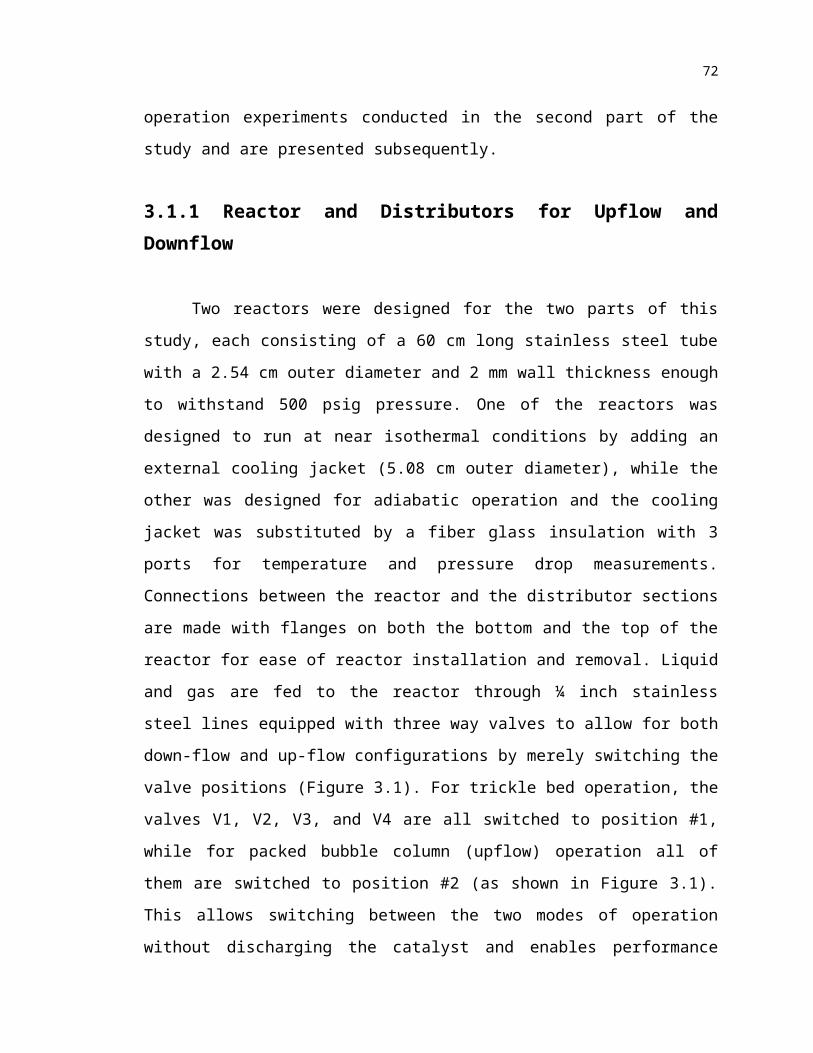
4.1.1 Effect of Reactant Limitation on Comparative Performance of

TBR and PBCAt low pressure (30 psig) and high feed concentration of a-methylstyrene (CBi=

7.8 %v/v), the reaction is gas limited ( = 8.8). In this case, downflow performed better

than upflow reactor as shown in Figure 4-1. This is due to the nature of the

hydrogenation reactions which are typically hydrogen (gas reactant) limited at low

pressure (at or just above atmospheric) and high a-methylstyrene concentrations

(Beaudry et al., 1987). It is obvious that this is due to low hydrogen solubility at these

pressures which reduces the external transport rates of hydrogen. In downflow mode of

operation, the catalyst particles are not fully wetted at the liquid flow rates used (Figure

4-11 shows contacting efficiency calculated using the correlation of Al-Dahhan and

Dudukovic (1995)). This facilitates the access of the gas reactant to the pores of the

68

catalyst on the externally dry parts, and reduces the extent of gas limitation compared to

fully wetted pellets in the upflow reactor. The result is a higher conversion in downflow

than in the upflow mode of operation. In case of upflow, since the catalyst is almost

completely wetted, the access of gaseous reactant to the catalyst sites is limited to that

through liquid film only. This provides an additional resistance for the gaseous reactant

(especially at high space time i.e., low liquid flow rate) and results in conversion lower

than that obtained in downflow. This effect is more prominent at higher liquid reactant

feed concentrations, due to the larger extent of gas limitation at such conditions (higher

values). As liquid mass velocity increases (space time decreases), the downflow

performance approaches that of upflow due to catalyst wetting efficiency approaching

that of upflow (contacting efficiency approaches 1 as seen in Figure 4-11).

As the reactor pressure increases and the feed concentration of a-methylstyrene

decreases, the value of decreases and the reaction approaches liquid limited behavior as

postulated earlier. This is reflected in a complete reversal in performance at higher

pressures and at low a-methylstyrene concentration (Figure 4-2), where the performance

of upflow becomes better than downflow. This is because under these conditions the

catalyst in downflow is still partially wetted (since at the operating gas velocities and gas

densities (hydrogen), high pressure only slightly improves wetting in downflow (Figure

4-11 based on Al-Dahhan and Dudukovic, 1995) while catalyst is fully wetted in upflow.

In a liquid limited reaction, liquid reactant conversion is governed by the degree of

catalyst wetting, and since upflow has higher wetting (100 %) than downflow, it

outperforms downflow (Figure 4-2). As the liquid mass velocity increases, and the

contacting efficiency of downflow approaches 100 %, the performance of the two

reactors approaches each other, as evident in Figure 4-2 at low space times. Thus, as

pressure is increased from 30 to 200 psig, and feed concentration of a-methylstyrene is

decreased from 7.8% to 3.1%(v/v), the reaction is transformed from a gas-limited ( =

8.8) to a liquid-limited regime ( = 0.8). The criterion () is dependent on two factors

69

(apart from the diffusivity ratio), pressure (hydrogen solubility) and feed concentration of

the liquid reactant (a-methylstyrene) (as discussed in Section 2.1.2). Further insight into

the gas and liquid limitation can be obtained by investigating these two contributions

individually for the set of operating conditions examined.

70

Figure 4-. Trickle Bed and Up-flow Performance at CBi=7.8%(v/v) and Ug =4.4 cm/s at

30 psig.

Figure 4-. Comparison of Down-flow and Up-flow Performance at CBi=3.1%(v/v) at

200 psig.

71

4.1.2 Effect of Reactor Pressure on Individual Mode of Operation

As reactor pressure increases, the performance of both upflow and downflow

improves due to increase in gas solubility, which helps the rate of transport to the wetted

catalyst (in both modes) and improves the driving force for gas to catalyst mass transfer

to the inactively wetted catalyst in the downflow mode. At low feed concentration of the

liquid reactant (a-methylstyrene (3.1%v/v)) and at high pressure (>100 psig), the

reaction becomes liquid reactant limited (or liquid reactant affected) as can be seen from

Figures 4-3 and 4-4 where no further enhancement is observed when pressure is

increased from 100 to 200 psig (where drops from 1.5 at 100 psig to 0.8 at 200 psig).

This means that any further increase in the reactor pressure and hence liquid phase

hydrogen concentration, will have minimal effect since hydrogen is not the limiting

reactant anymore.

To confirm the above observation the reaction was studied at higher feed

concentration of a-methylstyrene (4.8 %v/v) in order to determine whether gas limited

behavior is observed at higher values. The performance indeed improves when pressure

is increased from 100 to 200 psig (Figures 4-5) implying that the reaction is not yet

completely liquid limited at this feed concentration at 100 psig operating pressure

(=2.44). Liquid limitations are felt at pressures above 200 psig ( =1.3) at this feed

concentration, whereas the reaction is indeed liquid limited at lower a-methylstyrene

concentration (3.1%v/v) even at lower pressures as noted previously in Figures 4-3 and

4-4. Both upflow and downflow conversion increases with increasing pressure, primarily

due to increase in the solubility of the gaseous reactant as the pressure increases. A

significant improvement in performance (conversion) occurs when pressure is changed

from 30 to 100 psig as compared to the change in conversion when pressure changes

from 100 to 200 psig. This confirms that the effect of pressure diminishes when liquid

limitation is approached (as approaches 1.0 from above (Figure 4-5)).

72

Figure 4-. Effect of Pressure at Low a-methylstyrene Feed Concentration on Upflow

Reactor Performance.

Figure 4-. Effect of Pressure at Low a-methylstyrene Feed Concentration (3.1% v/v) on

Downflow Performance.

73

Figure 4-. Effect of Pressure at Higher a-methylstyrene Feed Concentration on

Downflow Performance.

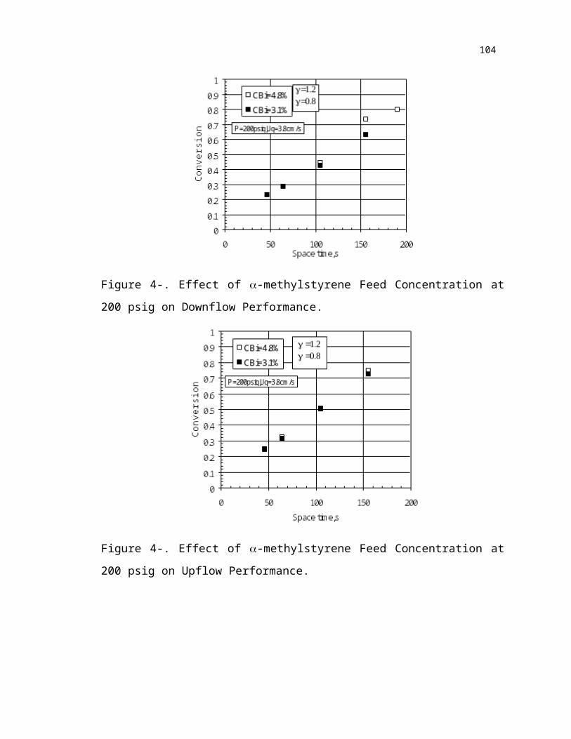
4.1.3 Effect of Feed Concentration of a-methylstyrene on Individual

Mode of Operation

Atmospheric pressure hydrogenation of a-methylstyrene has been known to

behave as a zero order reaction with respect to a-methylstyrene and first order with

respect to hydrogen (El-Hisnawi et al., 1982; Beaudry et. al, 1986). Our observations

confirm this observation at 30 psig as well as at 100 psig, the reaction is zero order with

respect to a-methylstyrene as shown in Figures 4-6 and 4-7 for upflow and downflow,

respectively. An inverse proportionality of conversion with liquid reactant feed

concentration (typical of zero order behavior) is observed especially at higher liquid flow

rates (lower space times). At lower liquid flow rates, at 100 psig the zero order

dependence appears to vanish and a first order dependence (due to a-methylstyrene

transport or intrinsic rate limitations), i.e., conversion independent of feed concentration,

is observed. Beaudry et al. (1987) also observed positive order with respect to the liquid

74

reactant at low liquid velocities (much higher space times) due to alpha-methylstyrene

affecting the rate. This shift in feed concentration dependence is confirmed by data at

higher pressure (200 psig, Figures 4-8 and 4-9). When liquid limitation is observed there

is no effect of feed concentration on the conversion in either mode of operation, as can be

seen in Figure 4-8 and 4-9. This is a consequence of the intrinsic rate limitation that

shows up as a first order dependence making conversion independent of feed

concentration (see also Appendix A for high pressure intrinsic rate data).

75

Figure 4-. Effect of a-methylstyrene Feed Concentration at 100 psig on Upflow

Performance.

Figure 4-. Effect of a-methylstyrene Feed Concentration at 100 psig on Downflow

Performance.

76

Figure 4-. Effect of a-methylstyrene Feed Concentration at 200 psig on Downflow

Performance.

Figure 4-. Effect of a-methylstyrene Feed Concentration at 200 psig on Upflow

Performance.

77

4.1.4 Effect of Gas Velocity and Liquid-Solid Contacting Efficiency

At low gas and liquid mass velocities, the level of interaction between the gas and

liquid phases is expected to be minimal in the downflow mode of operation. In case of

upflow, the effect of gas velocity on gas-liquid mass transfer is expected due to changing

interfacial area for transport with changing gas velocity. This would however only be

influential in determining the performance if the gas-liquid mass transfer were limiting

the overall reaction. The influence of gas velocity on the performance of both upflow and

downflow reactors is shown in Figure 4-10. The effect of gas velocity on reactor

performance was also examined for both upflow and downflow reactors. A significant

effect was not observed in the range of the gas velocities studied (3.8-14.4 cm/s, i.e., gas

Reynolds number in the range of 6-25) on either downflow or upflow performances at all

the feed concentrations and pressures tested. This is in agreement with earlier

observations of Goto et. al (1993). Experimental pressure drop measurements were also

made for both modes of operation during the reaction runs. The data obtained (shown in

Figure 4-11) indicates higher pressure drops for upflow at both ends of the pressure

range covered (30 and 200 psig) than for downflow, which is in agreement with

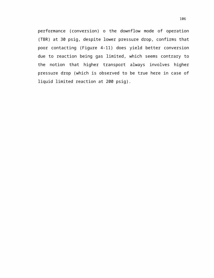
expectation and the pressure drop data reported in the literature. The better performance

(conversion) o the downflow mode of operation (TBR) at 30 psig, despite lower pressure

drop, confirms that poor contacting (Figure 4-11) does yield better conversion due to

reaction being gas limited, which seems contrary to the notion that higher transport

always involves higher pressure drop (which is observed to be true here in case of liquid

limited reaction at 200 psig).

78

Figure 4-. Effect of Gas Velocity on Reactor Performance at 100 psig.

Figure 4-. Pressure Drop in Downflow and Upflow Reactors and Contacting Efficiency

for Downflow Reactor at 30 and 200 psig.

79

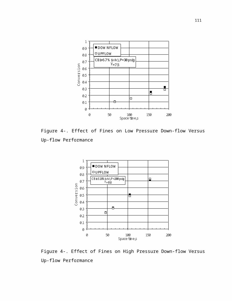
4.2 Comparison of Down-flow (TBR) and Up-flow (PBC) Reactors with Fines Fines (nonporous inert particles, order of magnitude smaller than catalyst pellets

packed only in the voids of the catalyst) were used to investigate the performance of the

two modes of operation using the same reaction in an attempt to demonstrate the

decoupling of hydrodynamic and kinetic effects. A way to establish this decoupling is to

use the upflow and downflow modes, which are intrinsically hydrodynamically different

(as discussed earlier), and asses whether fines can indeed yield the "true" kinetic behavior

(more properly called "apparent" rates on catalyst pellets of interest, i.e., rates unmasked

by external transport resistances and hydrodynamic effects). The two extreme cases

discussed before, i.e., gas limitation (downflow performance better than upflow, Figure

4-1), and liquid limitation (upflow performance better than downflow, Figure 4-2) are

now conducted in the presence of fines. Figures 4-12 and 4-13 show the performance of

both reactors when the bed is diluted with fines. It can be seen by comparing Figure 4-12

with Figure 4-1 and Figure 4-13 with Figure 4-2 that fines have eliminated the disparities

between the two modes of operation even in the extreme cases of reactant limitation.

This is primarily due to the fact that fines improve liquid spreading considerably and

achieve comparable (and almost complete) wetting in both modes of operation. It must

be noted that Figures 4-1 and 4-12, or Figures 4-2 and 4-13, could not be directly

superimposed due to slightly different catalyst activity obtained after repacking the bed

with fines and catalyst and reactivating it. Nevertheless, fines have successfully

decoupled the hydrodynamics and apparent kinetics, and the data with fines reflect the

kinetics in the packed bed under "ideal" liquid distribution conditions. It can be observed

in Figure 4-12 that at low liquid flow rate and low pressure (gas limited reaction), a

trickle bed with fines still performs slightly better than upflow with fines, which

80

indicates that the degree of wetting is still not complete in downflow resulting in some

direct exposure of the internally wetted but externally dry catalyst to the gas . This may

be due to the fact that at low liquid flow rate even with fines , the catalyst is not

completely externally wetted (Al-Dahhan and Dudukovic, 1995). At high pressure (liquid

limited reaction) Figure 4-12 reveals identical performance of both reactors where

complete wetting is achieved in both modes.

Since we studied the impact of the two factors, pressure and feed concentration

on the performance without fines, the same study was conducted for the bed diluted with

fines.

81

Figure 4-. Effect of Fines on Low Pressure Down-flow Versus Up-flow Performance

Figure 4-. Effect of Fines on High Pressure Down-flow Versus Up-flow Performance

82

4.2.1 Effect of Pressure in Diluted Bed on Individual Mode of Operation

The effect of pressure on the performance of both modes of operation in beds

with fines is illustrated in Figures 4-14 and 4-15. At higher pressure the performance of

both upflow and downflow is better than that at low pressure. This observation is also

consistent with the data obtained without fines. The pressure dependence observed is as

expected due to the increase in gas solubility with increased pressure. The same rate

dependence in hydrogen concentration was reported by Beaudry et al. (1987) as was also

observed in slurry experiment at both pressures as discussed in Appendix A and reported

by El-Hisnawi et al. (1982). Beaudry et al. (1987) observed some liquid limitation effects

(on the externally dry areas of the catalyst resulting in somewhat lower rate than

predicted by gas limited conditions) at low liquid mass velocity (high space time) even

for the gas limited case. These were not seen at the lower space times examined in this

study.

4.2.2 Effect of Feed Concentration in Diluted Bed on Individual Mode of

Operation

At 30 psig, liquid reactant conversion is higher at lower feed concentration of a

methyl styrene (lower 2 curves for downflow (Figure 4-14) and upflow (Figure 4-15). At

higher reactor pressure, there is no effect of feed concentration (upper 2 curves, Figure 4-

14 and 4-15). This was also observed for the reactors without fines and explained on the

basis of liquid limitation in the previous section. The fact that it is observed with fines

confirms the feed concentration dependence (of performance) in case of gas and liquid

limited reaction.

Fines have been shown to successfully decouple the hydrodynamics and reaction

effects, and can yield true apparent kinetic data in the packed bed under "ideal" liquid

distribution conditions. Both gas and liquid limited conditions were investigated and

identical performance was shown under all conditions studied, implying that using fines

83

is the recommended strategy to be used in obtaining data for scale-up or during scale-

down.

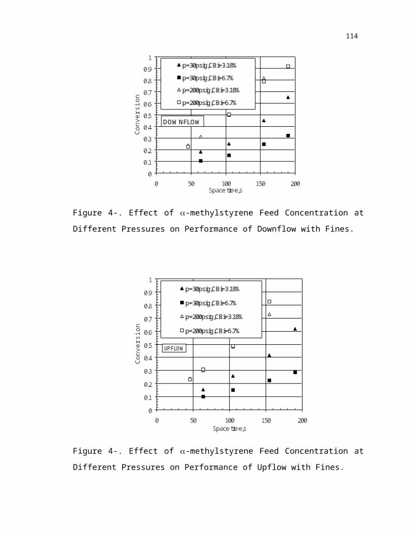
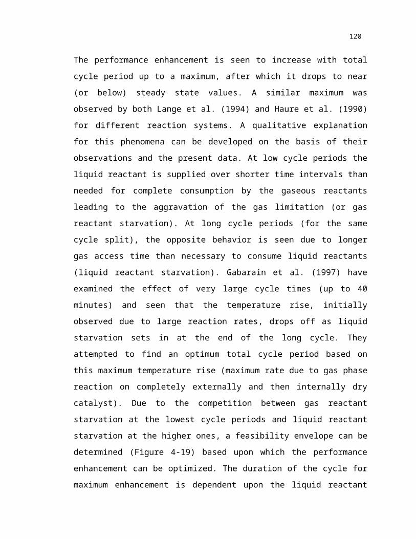
Figure 4-. Effect of a-methylstyrene Feed Concentration at Different Pressures on

Performance of Downflow with Fines.

84

Figure 4-. Effect of a-methylstyrene Feed Concentration at Different Pressures on

Performance of Upflow with Fines.

4.3 Unsteady State Experiments in TBRThe objectives outlined in Chapter 1 for the study of unsteady state operation

were to conduct experiments to examine the effect of gas and liquid reactant limitation as

well as cycling parameters such as total cycle period, cycle split, and cycling frequency

(as described in Section 3.2.3) on TBR performance. Comparison of the data obtained (as

listed in Appendix F) is reported with the few data available in the literature on similar

systems.

4.3.1 Performance Comparison for Liquid Flow Modulation under Gas

and Liquid Limited Conditions

Trickle bed performance was investigated for the two cases of interest, (i) gas

reactant limitation, and (ii) liquid reactant limitation, by changing operating pressure and

feed concentration. Performance under unsteady state operation was determined by

85

evaluating the flow averaged conversion over several cycles of operation according to the

procedure outlines in Section 3.2.3. Based on several trial runs, a total cycle time of 60 s

and a cycle split of 0.5 were chosen for this set of experiments with liquid ON/OFF flow

(see Figure 4-26 for liquid mass velocities corresponding to the space times investigated).

Under near liquid-limited conditions (i.e., high pressure and low feed concentrations) no

enhancement is observed with this modulation strategy, except at very low liquid mass

velocities (high mean space times (= VR/QL(mean)). At high liquid mass velocity, the

catalyst is well irrigated and any advantage due to better wetting under unsteady state is

not feasible. This can be qualitatively seen by examining the convex shape of the

contacting efficiency curve (Figure 4-26) which would yield better catalyst wetting under

steady state conditions and hence better performance under steady state conditions. This

analysis cannot however be applied at low liquid mass velocity where the unsteady state

wetting and replenishment of stagnant liquid pockets with fresh liquid reactants can

make enhancement possible. Under these conditions, the bed is poorly irrigated and the

disadvantage due to liquid maldistribution (not seen in steady state contacting efficiency

plot as shown in Figure 4-26) can be overcome by the high flow rate liquid (Figure 4-16,

at high space times).

At low space times (high mass velocity, Figure 4-16), performance enhancement

is not seen under laboratory conditions due to several factors such as small reactor

diameter, good distributor, all leading to good catalyst wetting (as seen in Figure 4-26).

The conditions investigated in the present experiments correspond to fairly high liquid

hourly space velocities (LHSV) in comparison with industrial trickle beds, where this

maldistribution effect may be seen to be more pronounced. LHSV varied from 3 to 15 in

our experiments as compared to 1.5 to 10 used in industrial reactors.

In case of gas limited conditions (i.e., at low operating pressures and high feed

concentration), it can be seen in Figure 4-17 ( ~ 25) that unsteady state performance

(conversion) is significantly higher than that under steady state conditions at all space

86

times. This case illustrates the conditions of a liquid reactant full catalyst and enhanced

supply of the gaseous reactant leading to better performance. The observed enhancement

improves as the extent of partial wetting is increased as seen at higher space times (lower

liquid mass velocities). This also corroborates the findings of Lange et al. (1994) and

Castellari and Haure (1995) that under severe gas limitation (due to 50 % (v/v) and 100

% pure liquid reactants in their studies respectively) enhancement is feasible. Castellari

and Haure (1995) explored this enhancement further by increasing the total cycle time to

allow for complete internal drying of catalyst and corresponding large temperature

increase and semi-runaway conditions. This was not feasible in the present study, but

enhancement due to higher gas supply was expected to increase by increasing the gaseous

reactant supply and lower liquid ON times. A small exothermic contribution was also

observed during unsteady state operation here with maximum bed temperatures reaching

~ 6 oC higher than steady state temperatures.

87

Figure 4-. Comparison of Steady and Unsteady State Performance at Conditions

Approaching Liquid Limitation ( < 4)

Figure 4-. Comparison of Steady and Unsteady State Performance under Gas Limited

Conditions ( ~25)

88

4.3.2 Effect of Modulation Parameters (Cycle Period and Cycle Split) on

Unsteady State TBR Performance

To explore whether further performance enhancement is achievable for the gas

reactant limited case by increasing gaseous reactant supply to the catalyst, a constant

liquid mean flow was chosen (Space time = 660 s, L= 0.24 kg/m2s) and cycle split ()

was varied (to vary the ratio of the gas to liquid access times). It can be seen that further

enhancement was indeed possible the cycle split was lowered from steady state ( = 1) to

a split of = 0.25, the performance improved by as much as 60% over steady state at the

same mean liquid mass velocity (Figure 4-18). This improvement continues up to the

point where liquid limitation sets in at very low cycle split (indicating that the liquid is

completely consumed during a time interval shorter than the OFF time of the cycle),

beyond which the performance will be controlled by liquid reactant supply. This implies

that performance improvement can be maximized by choosing an appropriate cycle split

(at a given liquid mass velocity and total cycle period).

The effect of the total cycle period was investigated at the cycle split () value of

0.33, where performance enhancement was observed to be significant (Figure 4-18). The

performance enhancement is seen to increase with total cycle period up to a maximum,

after which it drops to near (or below) steady state values. A similar maximum was

observed by both Lange et al. (1994) and Haure et al. (1990) for different reaction

systems. A qualitative explanation for this phenomena can be developed on the basis of

their observations and the present data. At low cycle periods the liquid reactant is

supplied over shorter time intervals than needed for complete consumption by the

gaseous reactants leading to the aggravation of the gas limitation (or gas reactant

starvation). At long cycle periods (for the same cycle split), the opposite behavior is seen

due to longer gas access time than necessary to consume liquid reactants (liquid reactant

starvation). Gabarain et al. (1997) have examined the effect of very large cycle times (up

89

to 40 minutes) and seen that the temperature rise, initially observed due to large reaction

rates, drops off as liquid starvation sets in at the end of the long cycle. They attempted to

find an optimum total cycle period based on this maximum temperature rise (maximum

rate due to gas phase reaction on completely externally and then internally dry catalyst).

Due to the competition between gas reactant starvation at the lowest cycle periods and

liquid reactant starvation at the higher ones, a feasibility envelope can be determined

(Figure 4-19) based upon which the performance enhancement can be optimized. The

duration of the cycle for maximum enhancement is dependent upon the liquid reactant

concentration as seen in the experiments of Lange et al. (1994) (cycle period ~ 7.5

minutes for ~ 50 % v/v of alpha-methylstyrene) under similar operating conditions. This

maximum could be quantified by a complex function of an effective parameter (under

dynamic conditions) and the effect of cycle split and liquid mass velocity if transient

variation of concentration is known accurately. The above effects of cycle split and total

cycle period were examined at a constant liquid mass velocity. Due to the strong

dependence of catalyst wetting and reaction rate (both steady and unsteady), on liquid

mass velocity (also referred to as amplitude of the flow modulation) its effect is

important from the point of view of commercial scale application and is examined next.

90

Figure 4-. Effect of Cycle Split () on Unsteady State Performance under Gas Limited

Conditions

Figure 4-. Effect of Total Cycle Period () on Unsteady State Performance under Gas

Limited Conditions

91

4.3.3 Effect of Amplitude (Liquid Mass Velocity) on Unsteady State

TBR Performance

The feasibility envelope (region where performance enhancement is possible, as

shown in Figure 4-19) as discussed in Section 4.3.2 and observed in literature is strongly

dependent on the relative supply of gaseous and liquid reactants. Gaseous reactant access

is governed by the extent of external catalyst wetting (which depends on liquid flow rate)

and the formation of dry areas (which depends on evaporation rate). Castellari and Haure

(1995) examined the catalyst drying phenomenon in their experiments which they

attributed to complete external and internal evaporation of liquid (until liquid reactant is

completely consumed). However, all of their experiments were conducted at the same

mean liquid mass velocity (~ 10 times higher than in the present study) at which the

steady state wetting is complete. The change in catalyst external wetting due to

evaporation in the present study is not large (compared to that observed by Castellari and

Haure (1995)) as compared to that due to change in flow with time. It is thus important

to explore whether the feasibility region for enhancement can be altered with changing

liquid mass velocity. Two mean liquid mass velocities at which wetting should have the

most effect (lowest mass velocity possible, see Figure 4-26) were examined (at a cycle

split of 0.25). The results presented in Figure 4-20 compare normalized enhancement

(conversion at unsteady state over that at steady state). A significantly higher

enhancement is observed by lowering the mean liquid mass velocity. At a mass velocity

of 0.137 kg/m2s, a similar feasibility envelope is seen as in Figure 4-19 which ends in

degradation of performance to below steady state values at higher cycle periods due to

depletion of the liquid reactant (liquid starvation onset as discussed in the previous

section). The lower liquid mass velocity allows more time for liquid reactant supply

(higher mean space times) to the catalyst. This is reflected in the shift in the liquid

starvation to even higher total cycle periods (Figure 4-20), while the gas starvation side

remains unchanged (similar to that observed in Figure 4-19). The higher maximum

92

enhancement at lower liquid mass velocity (Figure 4-20) clearly indicates the trend

towards the limit of maximum possible enhancement (the ideal case of zero flow of

liquid reactant and complete conversion).

Figure 4-. Effect of Liquid Mass Velocity on Unsteady State Performance under Gas

Limited Conditions

93

4.3.4 Effect of Liquid Reactant Concentration and Pressure on

Performance

The two key parameters which decide the extent of gas or liquid reactant

limitation are the liquid reactant feed concentration and operating pressure. The

combined effect of these was discussed in Section 4.3.1 for two sets of steady and

unsteady state performance data corresponding to the gas limited and liquid limited

extremes. It was shown that with the ON/OFF liquid flow modulation strategy,

performance enhancement was possible under gas limited conditions (Figure 4-17). The

effect of individual contributions of pressure and liquid reactant feed concentration under

gas limited conditions needs to be carefully examined to determine the exact cause-effect

relationships in performance enhancement. The effect of liquid reactant feed

concentration was examined under gas limited conditions by evaluating the enhancement

at different cycle splits. With the increase in gas limitation due to higher liquid reactant

feed concentration, we would expect higher enhancement due to flow modulation at

higher liquid reactant feed concentration. However, this is not observed as expected

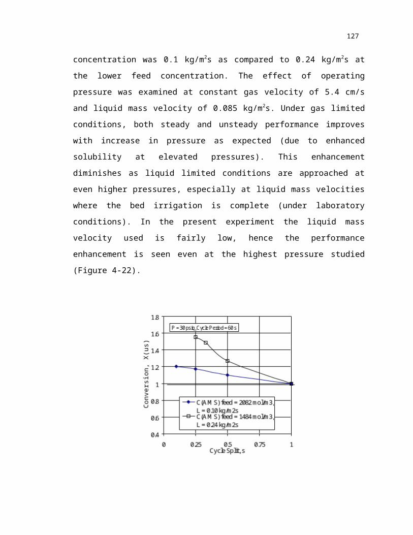
(Figure 4-21). Since the absolute value of the conversion at higher feed concentrations is

lower (due to gas reactant limitation), the enhancement seen is not as high even if lower

mean liquid mass velocity was used. The liquid mass velocity used at the higher liquid

reactant feed concentration was 0.1 kg/m2s as compared to 0.24 kg/m2s at the lower feed

concentration. The effect of operating pressure was examined at constant gas velocity of

5.4 cm/s and liquid mass velocity of 0.085 kg/m2s. Under gas limited conditions, both

steady and unsteady performance improves with increase in pressure as expected (due to

enhanced solubility at elevated pressures). This enhancement diminishes as liquid limited

conditions are approached at even higher pressures, especially at liquid mass velocities

where the bed irrigation is complete (under laboratory conditions). In the present

94

experiment the liquid mass velocity used is fairly low, hence the performance

enhancement is seen even at the highest pressure studied (Figure 4-22).

Figure 4-. Effect of Liquid Reactant Feed Concentration on Unsteady State Performance

under Gas Limited Conditions

95

Figure 4-. Effect of Operating Pressure on Unsteady State Performance under Gas

Limited Conditions

96

4.3.5 Effect of Induced Flow Modulation (IFM) Frequency on Unsteady

State Performance

Liquid ON/OFF flow modulation can be considered as square wave cycling about

the mean flow for the case with a cycle split of 0.5. Conversion under periodic conditions

can then be used to examine the dominant time scales affected by induced flow

modulation (IFM) by looking at the frequency () dependence of flow averaged

conversion. Both Figures 4-23 and 4-24 show performance enhancement as a function of

the IFM frequency with similar trends seen at different pressures, feed concentrations,

and even for a case of non-square wave pulsing ( = 0.2). The performance in both cases

shows degeneration of the enhancement at low frequencies tending to the steady state

operation at zero frequency. But as frequency is increased, the conversion reaches a clear

maximum improvement point. Ritter and Douglas (1970) observed a similar frequency

dependence for dynamic experiments in stirred tanks and attributed the maximum to the

resonance frequency of the rate controlling process. All transport processes typically

have a natural frequency corresponding to their characteristic time scale. Gas-liquid

transport in trickle beds corresponds to 0.2 to 0.8 Hz (at low pressures), liquid-solid

transport corresponds to 0.5 to 2 Hz (Gianetto and Silveston, 1986; Astarita, 1997),

whereas catalyst level reaction-diffusion processes correspond typically to much lower

frequency (larger time scale) depending upon intrinsic rates in pellets (Lee and Bailey,

1974; Kouris et al, 1998). Typical industrial reactions in trickle bed reactors have been

reported to correspond to a frequency range of 0.01 to 0.1 Hz (Wu et al., 1995). Natural

pulsing occurs in trickle beds at high liquid flows and displays frequencies of 1 to 10 Hz,

at which external transport is significantly improved (Blok and Drinkenberg, 1982; Wu

et al., 1995). The present IFM frequencies are much lower than those observed under

natural pulsing. The frequency dependence of the performance (Figure 4-23 and 4-24)

shows that the highest effect of IFM can be observed at low frequencies ( ~ 0.01 Hz) at

97

which catalyst level processes could be predominantly affected to obtain the observed

enhancement. Some effect on external transport processes can also be seen (in Figures 4-

23 and 4-24) where enhancement corresponding to their natural frequencies is observed.

This opens up the possibility of selectivity enhancement and control for complex reaction

schemes by controlling reactant supply by the proper choice of the IFM frequency for the

desired reactant (Wu et al., 1995). The low enhancement seen at both ends ( 0 and

) can be explained on the basis of the frequency analysis similar to that done by Lee

and Bailey (1974). The very low IFM frequency ( 0) corresponds to an equilibrium

state or pseudo steady state, where the reaction transport processes have time to catch up

with the modulated variable (flow in this case) and the overall system behaves as a

combination of discrete steady states. On the other hand at high IFM frequency ( ),

the input fluctuations are so rapid that none of the reaction-transport processes in the

system can respond fast enough to the induced flow modulation (IFM), and, no gain in

performance due to the modulated variable is again not feasible. This has been confirmed

by pellet scale reaction-diffusion simulations with time varying boundary conditions (at

high frequencies) by Lee and Bailey (1974) and Kouris et al. (1998). They have shown

that at low frequencies, the catalyst has a chance to react to external changes and effect of

time variation propagates to the interior of the catalyst, while at higher frequencies the

system (catalyst) cannot relax to the rapidly changing external conditions and

performance corresponding to a stationary state (time averaged wetting) is observed.

98

Figure 4-. Effect of Cycling Frequency on Unsteady State Performance under Gas

Limited Conditions

Figure 4-. Effect of Cycling Frequency on Unsteady State Performance under Gas

Limited Conditions

99

4.3.6 Effect of Base-Peak Flow Modulation on Performance

For the case of liquid limited conditions (i.e., at high pressure and low feed

concentrations) the use of complete absence of liquid during the OFF part of the cycle (as

done in ON-OFF flow modulation) is not beneficial, as this would worsen the liquid

limitation. This was confirmed in the discussion in Section 4.3.1 and experimental

observations of Lange et al. (1994). Instead of the conventional ON-OFF liquid flow, a

low base flow (with magnitude similar to the mean operating flow) is introduced during

the OFF part of the cycle (referred to as BASE flow) with a periodic high flow slug

introduced for a short duration (referred to as PEAK flow) to improve liquid distribution

and open up multiple liquid flow pathways during the rest of the cycle (Gupta, 1985;

Lange et al., 1994). The cycle split () here is the fraction of the cycle period during

which the high flow rate slug is on (typically chosen to be very short).

Tests were conducted at a cycle split of 0.1 and cycle times varying from 30 to

200 s at an operating pressure of 150 psig and low liquid reactant feed concentration

(C(AMS) feed = 784 mol/m3) to ensure liquid limited conditions. This strategy is shown to

yield some improvement over steady state performance (Figure 4-25, < 1.2), although

this is not as high as observed under gas limitation. The maximum enhancement

observed here was 12 % as against 60 % in case of gas limited conditions. The limited

enhancement is primarily due to intrinsically better flow distribution in small laboratory

reactors, which would not be the case in typical pilot or industrial reactors where much

higher enhancement can be anticipated.

100

Figure 4-. Unsteady State Performance with BASE-PEAK Flow Modulation under

Liquid Limited Conditions

Figure 4-. Effect of Liquid Mass Velocity on Steady State Liquid-Solid Contacting

Efficiency

L (peak)

L (mean) = L (peak)+(1-) L (base)

, (sec)

(1-) L (base)

L (mean)

101

Chapter 5. Modeling Of Trickle Bed Reactors 5.1 Evaluation of Steady State Models for TBR and PBC

The qualitative analysis presented in the discussion of the experimental results in

Section 4.1 on the basis of reactant limitation, liquid-solid contacting, and effect of

pressure on kinetics was verified by comparison with predictions of some of the existing

models as discussed in this section. A history of the model development for trickle bed

reactors was presented in Chapter 2 and the salient features of each model were presented

in Table 2.3. Based on the discussion therein, two models (developed at CREL), one with

reactor scale equations (El-Hisnawi, 1982) and the other with pellet scale equations

(Beaudry, 1987) were chosen to compare predictions to experimental data. The key

distinction in modeling downflow and upflow are the values of mass transfer parameters

(evaluated from appropriate correlations) and the catalyst wetting efficiency. The

solution of partially wetted pellet performance is required for downflow and fully wetted

pellets can be assumed for upflow. The effect of liquid mass velocity on simulated gas-

liquid and liquid-solid transport in both reactors was required. These were evaluated

from correlations proposed in the literature for the reactor under consideration. The

intrinsic kinetics required was obtained from slurry experiments as discussed in Section

4.1 and Appendix A.

5.1.1 Reactor Scale Model (El-Hisnawi et al., 1982)

The El-Hisnawi et al. (1982) model was originally developed for a low pressure

trickle bed reactor to account for rate enhancement for gas limited reaction due to

102

externally inactively wetted areas. The model was proposed in the form of heterogeneous

plug flow equations for the limiting reactant. The surface concentration of the limiting

reactant is obtained by solution of the reaction transport equation at the catalyst surface.

This is substituted into the plug flow equation of the non-limiting reactant to obtain its

profile (Table 5.1). For example, when A (gaseous reactant, hydrogen) is the limiting

reactant, its surface concentration is solved for, and, rate evaluated on its basis is

substituted in the plug flow equation for concentration of B (liquid reactant, alpha-

methylstyrene) to obtain the conversion of B at each velocity specified. Analytical

solutions were derived for the first order kinetics for the equations at low pressures. At

high pressure, however, the reaction was observed to be liquid reactant B limited with

non-linear kinetics (given in the Langmuir–Hinshelwood form in Appendix A). Surface

concentration of B was solved for from the non-linear rate equation (in Table 5.1) to get

the surface concentration. Then differential equation for the concentration of species B is

then solved numerically to get the concentration profile of B and reactor exit conversion

at each space time. The pellet effectiveness factor can be determined from the Thiele

modulus but was used here as a fitting parameter based on its value at one of the cases

and used for the rest. This was done due to the uncertainty in the catalyst activity (rate

constant) and the effective diffusivity values at high pressures. The liquid-solid

contacting efficiency was determined at low pressure by the correlations developed by

El-Hisnawi (1981) and at high pressure using the correlation of Al-Dahhan and

Dudukovic (1995). The upflow reactor was assumed to have completely wetted catalyst

in all cases. For downflow gas-liquid mass transfer coefficient was obtained from

Fukushima and Kusaka (1977) correlation, liquid-solid mass transfer coefficient was

calculated from Tan and Smith (1980), and gas-solid mass transfer coefficient was

estimated by the method of Dwiwedi and Upadhyay (1977). For upflow prediction, the

gas-liquid mass transfer coefficients were obtained from the correlation by Reiss (1967),

and, liquid-solid mass transfer coefficients from the correlation by Spechhia (1978). The

103

variation of the mass transfer coefficients calculated from the above correlations with

space time is shown in Figure 5-5. The predictions of the El-Hisnawi model at low

pressure (gas limited) compare well with the downflow experimental data as shown in

Figure 5-1. For the case of upflow performance, however, the model over predicts the

experimental data at low space time. This implies that the effect of external mass transfer

is felt in case of the predicted conversion profile for upflow, which is not observed

experimentally. The mass transfer correlations used typically predict higher values at

higher liquid velocity (lower space time) resulting in the higher predicted conversion at

low space times. At high pressure, liquid limited conditions, however, El-Hisnawi model

predictions compare well with the experimental data for upflow and downflow as shown

in Figure 5.2. The effect of mass transfer is not felt as much at high pressure and

predictions are qualitatively and quantitatively (within 5%) able to capture the

observed experimental behavior of both reactors.

104

Table 5. 1 Governing Equations for El-Hisnawi (1982) Model

Original model equations (gas limited conditions)

And

Boundary conditions:

Equilibrium feed

Non-Equilibrium feed

and

Model equations at high pressure (liquid limited conditions)

(boundary conditions are the same as at low pressure)

(for liquid reactant limitation)

105

Table 5. 2 Governing Equations for Beaudry (1987) Model

Pellet Scale Equations:

a) Low Pressure (Gas Reactant Limited) with rate first order in A.

Boundary conditions (Pellet):

(=0 for m<1)

(=0 for m<1)

Boundary conditions (Reactor):

Where,

106

Table 5-2. Governing Equations for Beaudry (1987) Model (continued)

b) High Pressure (Liquid Reactant (diffusional) Limitation for Langmuir-Hinshelwood rate form)

Boundary conditions:

For both case a) and b) above, the reactant conversion in general is given by

where

(at low pressure)

(at high pressure)

and overall effectiveness factor is given by

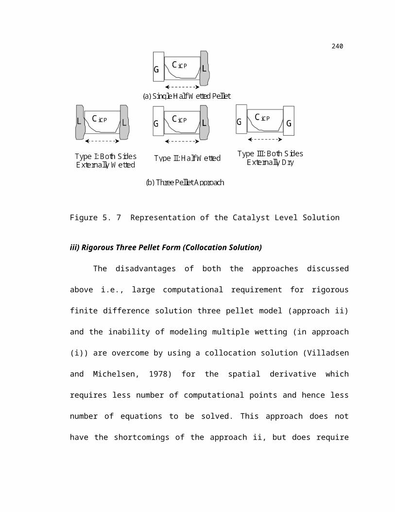
5.1.2 Pellet Scale Model (Beaudry et al., 1987).

Beaudry’s model considered the evaluation of catalyst pellet effectiveness subject

to different wetting conditions and substitution of the overall pellet effectiveness factor

into a simple plug flow equation to evaluate reactor conversion. The catalyst pellets were

modeled in the form of infinite slabs with the two sides exposed to either gas or liquid, or

a half-wetted pellet exposed to gas and liquid on one side only. At low pressure (gas

107

limited conditions), the gaseous reactant supplied from both sides of the pellet depletes to

almost zero within a short distance depending upon the extent of the gas reactant

limitation. Hence, the solution of the pellet effectiveness for downflow for the gas

limited case involved solution of both the dry and wetted side for a half wetted pellet,

and the solution of the completely wetted pellet (as shown Table 5-2). For the completely

dry pellet the effectiveness was zero since no liquid reactant could be supplied to this

pellet. The analytical solutions to this case for the reaction rate which is first order in

hydrogen are available in Beaudry et al. (1987) and were used to obtain the overall

effectiveness factor as a weighted average of the contacting and the effectiveness of each

type of pellet (as shown in Table 5-2). At high pressure (liquid limited conditions) the

solution is much more complicated due to the non-linear reaction rate which demands the

solution of the reaction diffusion equations for the externally wetted pellets on both sides

and the half wetted pellet only on the wetted side. Here, the value of is the point where

the liquid reactant depletes completely and is the boundary for the liquid reactant

concentration solution. This solution needs to be evaluated at each point in the reactor to

get a local effectiveness factor corresponding to the local concentration of the liquid

reactant. Instead of doing this as a coupled system of equation both on the pellet and

reactor scale, the pellet scale equations were solved at different bulk liquid reactant

concentrations and then fitted as a polynomial of pellet effectiveness as a function of

surface concentration. This polynomial is then used to solve the reactor scale equations

numerically to obtain conversion at each space time. Although this approach does not

require any fitted parameters as needed in the El-Hisnawi model, the rate constant was

similarly fitted to match the conversion at one space-time and used to compare with the

experimental data at all other space times. As can be seen from Figure 5-1 and 5-2, this

model predicts the observed data for down flow at low pressure and at high pressure

well, but not so well for up-flow especially at low pressure and high feed concentration.

The reason may be due to mass transfer correlations used for upflow which may predict a

108

lower performance (than observed experimentally) at high space times in the upflow

operating mode. This is also consistent with the predictions of El-Hisnawi model

discussed above.

The Beaudry et al. (1987) model predictions are also shown in Figure 5-1 and 5-2

for low and high pressure, respectively. As can be seen in the Figure 5-1, the Beaudry et

al. (1987) model predicts downflow performance at low pressure exactly as the El-

Hisnawi model does, but under-predicts upflow performance at higher space times (low

liquid velocities) due to the significant effect of mass transfer (as predicted by the

correlation used) particularly at high space times. At high pressure, on the other hand,

Beaudry's model predicts experimental data quite well both for downflow and upflow,

since the effect of mass transfer is not as pronounced as at low pressure.

The effect of the feed concentration on predictions of both models was also

examined for both downflow and upflow reactors as shown in Figures 5-3 and 5-4,

respectively. As mentioned earlier in the discussion, the predictions are almost identical

for both models for downflow and agree with experimental data. In both cases, however,

the inverse relationship of liquid feed concentration with conversion typical of low

pressure gas limited operation seen in the experiments is predicted correctly.

The predictions of the reactor scale and pellet scale models are

satisfactory for current conditions although there is a need for high pressure correlation

for mass transfer coefficient and interfacial area in order to predict performance with

greater certainty, especially in cases where the rate is affected significantly by external

mass transfer. The predicted performance of upflow and downflow for both models

presented and discussed in this section is seen to be strongly dependent on the reaction

system i. e., whether the reaction is gas or liquid limited under the conditions of

investigation. The laboratory reactors are often operated in the range of partially to fully

wetted catalyst and demonstrate the influence of wetting can be either detrimental or

beneficial, depending upon the reactant limitation. Models that account for these two

109

effects, i.e., reactant limitation and influence of catalyst wetting, can predict the

performance over the entire range of operating conditions. The intrinsic kinetics of the

reaction studied at different pressures is also important in obtaining good predictions.

Hence, for any given reaction it is recommended to study the slurry kinetics at the

specific operating pressure before any scale up or modeling is attempted. A rate

expression with different rate constants at each of the discrete pressures (as used here)

can be used to predict the trickle bed reactor data at the same pressures most accurately,

rather than using a general rate form which cannot fit all the data obtained at different

pressures. It must be mentioned that the reactor scale model failed to predict

experimental data well at the intermediate conditions (100 psig, ~ 1) when the reaction

is neither completely gas limited nor liquid limited (or switches from gas limited to

liquid limited at some location in the reactor) because the model assumptions were for

the extreme conditions of one reactant being limiting. Rigorous solution of the reactor

and pellet scale equations presented in the next section should be able to cover a general

case without the assumptions made here.

110

Figure 5. 1 Upflow and Downflow Performance at Low Pressure (gas limited condition):

Experimental data and model predictions

Figure 5. 2 Upflow and Downflow Performance at High Pressure (liquid limited

condition): Experimental data and model predictions

111

Figure 5. 3 Effect of Feed Concentration on Predicted Downflow Performance

Figure 5. 4 Effect of Feed Concentration on Predicted Upflow Performance

112

Figure 5. 5 Estimates of volumetric mass transfer coefficients in the range of operation

from published correlations (G-L (downflow) Fukushima and Kusaka (1977), L-S

(downflow) Tan and Smith (1980), G-L (upflow) Reiss (1967), L-S (upflow) Spechhia

(1978)).

113

5.2 Steady State Modeling of Systems with a Volatile Liquid Phase

A significant number of gas-liquid-solid catalyzed reactions in the petroleum

processing and chemical industries are carried out in trickle-bed reactors at conditions

under which substantial volatilization of the liquid phase can occur. Most of the models

available in the literature for trickle bed reactors are based on assumptions that are

invalid for complex reaction systems with volatile liquid species. Hence, a need exists for

comprehensive models that properly account for liquid phase volatilization under

conditions typically encountered in complex industrial processes. A review of the few

studies available in the literature on experiments and models for systems with volatile

liquids is presented. A rigorous model for the solution of the reactor and pellet scale

flow-reaction-transport phenomena based on multicomponent diffusion theory is

proposed. To overcome the assumptions in earlier models, such as non-volatile reactants,

dilute solutions, isothermal, isobaric operation, and constant phase velocities and

holdups, the Stefan-Maxwell formulation is used to model interphase and intra-catalyst

transport. The model predictions are compared with the experimental data of Hanika et

al. (1975) and with the predictions of a simplified model (Kheshgi et al., 1992) for the

test case of cyclohexene hydrogenation. Rigorous reactor and pellet scale simulations

carried out for both the liquid phase and gas phase reaction, as well as for intra-reactor

wet-dry transition (hysteresis and rate multiplicity), are presented and discussed.

Comparisons between various models, pitfalls associated with introducing simplifying

assumptions to predict complex behavior of highly non-ideal three phase systems, and

areas for future work are also suggested.MODEL DEVELOPMENT

114

Based on the observations reported in the above mentioned literature, the key features

that need to be incorporated into any model development for trickle bed reactor with

volatiles are:

1. Interphase transport and vapor-liquid equilibrium effects need to be modeled

rigorously.

2. Multi-component effects due to large inter-phase fluxes of mass and energy as well as

influence of varying concentration on transport of other components and the total

inter-phase fluxes need to be correctly modeled to maintain rigor.

3. The influence of volatilization and reaction on variation in holdup and velocity needs

to be incorporated.

4. Complete depletion of liquid reactants in the reactor should be modeled by correcting

or dropping the liquid phase equations based on computed holdup and temperature.

5. Partial catalyst wetting, either external or internal or both, should be incorporated.

6. The combined effects of imbibition, capillary condensation, liquid volatility, heats of

vaporization and reaction should be correctly solved for on the particle scale.

7. The existence of multiple steady states should be predicted by the model equations as

observed in the experimental results reported in literature.

The present model attempts to address the above requirements and extend the

models that account for some of the above effects. The level I and level II models

discussed below are catalyst and reactor level models and are extended to develop the

level III model as a combination of reactor and pellet scale models.

Level I: Pellet Scale Model

115

Kim and Kim (1981b) assumed that the macropores of the catalyst are filled with

vapor and have written reaction diffusion equations for slab geometry of the form

(1)

with standard boundary conditions. The reaction rate was then calculated as

(2)

and the heat generated was obtained directly from the rate. Their model considered

different effective diffusivity values, based on the state of their catalyst, as well as

different rate constants for the liquid and vapor phase reaction, which clearly gives the

multiplicity effects observed in their experiments.

As mentioned in the discussion above, Harold (1988) and Harold and Watson

(1993) considered partial internal wetting of a slab catalyst for a decomposition and

bimolecular reaction for which the effect of capillary condensation, evaporation,

reaction, and incomplete internal catalyst filling were used to investigate the multiplicity

of rates. The level III model developed in this study has incorporated the key features of

this model and they will be discussed along with the model equations in subsequent

sections.

Level II: Reactor Scale Model

In the model developed by LaVopa and Satterfield (1988), the reactor is chosen

as a series of stirred tanks alternated with flash units (which are not affected by the

reaction) for each of which there is a vapor and liquid inlet and outlet stream. This model

116

is suitable only for the case where large evaporation or thermal effects that will cause

change in liquid volatility are not present. Also, the effect of partial catalyst wetting and

existence of multiplicity has not been addressed by this model. Kheshgi et al. (1992)

developed a model based on a pseudo-homogeneous approach (for the reaction system of

Hanika et al. (1976)) coupled with a overall enthalpy balance that incorporates the

change in enthalpy of the liquid and vapor streams with reaction and phase change. The

resulting model equations given below by Equations 3 and 6, are solved in conjunction

with algebraic equilibrium and flow relations to obtain the velocity, conversion and

temperature profiles in the reactor. This model also incorporates partial catalyst wetting

and can predict multiplicity of rates as seen in experimental results of Hanika et al.

(1976). The authors have determined the rate parameters on the dry and wetted side of

the catalyst (kW, and kD respectively) as well as the bed thermal conductivity (l) and wall

heat transfer coefficient (U) for Hanika’s reactor based on their experimental data. Based

on Hanika et al.’s (1976) data, Kheshgi et al. (1992) assumed the order to be unity with

respect to cyclohexene for the dry pellet and unity with respect to hydrogen for the wet

pellet. The model equation for cyclohexane conversion along the reactor can be written

as:

(3)

where

(4)

(5)

117

The mole fractions in the vapor phase for components A (cyclohexene), B (hydrogen),

and C (cyclohexane) are then written in terms of vapor and liquid flows and used to

calculate liquid phase compositions using equilibrium relations. The energy balance for

the pseudo-homogeneous mixture is given by

(6)

with boundary conditions

at z=0, T=To, a = 0 and at z=L, dT/dz = 0 (7)

The wetting efficiency is calculated using the Mills and Dudukovic (1980) correlation,

but a large value of CW is chosen (CW =1000) so as to match the abrupt transition from

fully wetted to fully dry pellets in the bifurcation behavior observed by Hanika et al.

(1976). No distinction is made between external wetting and internal wetting of the

catalyst pellets, which means that an externally completely wetted is assumed to be

internally wetted pellet as well, and correspondingly, an externally dry pellet is assumed

to be internally dry as well (Kheshgi et al., 1992).

Level III: Reactor and Pellet Scale Multicomponent model (Combination of Level I

and II)

The level III model proposed here is a combination of a rigorous multi-

component model for the reactor scale and its extension to the pellet scale. The key

assumptions made are:

1. Only steady state profiles are modeled and any transient variation is ignored.

118

2. Variation of temperature, concentration, velocity and holdup in radial direction is

negligible as compared to the variation in axial direction.

3. All the parameter values are equal to the cross-sectionally averaged values and vary

only with axial location.

4. The catalyst pellets are modeled as half-wetted slabs exposed to liquid on one face

and gas on the other and partially internally filled as shown in Figure 1.

5. A change in state of internal wetting occurs due to a combination of the rate of

imbibition, evaporation, and pressure difference due to reaction in the internally dry

zone.

6. Pressure gradients can exist in the gas-filled zone, but not in the liquid-filled zone of

the catalyst pellet.

Level III Reactor Scale Equations

A two fluid approach is considered for the reactor scale model. Equations are

written for the gas and liquid phase mass, energy, and momentum transport with source

terms representing interphase fluxes that are modeled by multicomponent transport

across interfaces between the solid, liquid, and gas phase. For the special case of

complete volatilization of the liquid phase, the model is suitably modified by dropping

the liquid phase equations and corresponding interphase exchange terms. Since

multicomponent equations involve the solution of large number of non-linear

simultaneous equations coupled with the differential equations, the higher order terms in

the differential equations due to diffusion/dispersion are dropped to keep the problem to

119

an initial valued one (for computational suitability). For the reactor level equations

concerned, the number of unknowns for a nc component system are 10*nc+13 (as listed

in Appendix A) and the same number of equations are required to make the overall

problem consistent and solvable. The numbers in square brackets indicate the number of

such equations available for a system with nc number of components.

The continuity equations for the liquid and gas phase with total interphase fluxes as the

source terms are written as

[1] (8)

[1] (9)

Momentum equations (unexpanded form) for the liquid and gas phase with source term

contributions from gravity, pressure drop, drag due to solid, gas-liquid interaction and

added momentum due to interphase transport can be written as

[1] (10)

[1] (11)

[1] (12)

The momentum equations can be expanded and simplified using the continuity equations

and the assumption of identical interface and bulk velocity in each phase. The species

concentration equations written with source terms for absolute interphase fluxes for gas-

liquid, liquid-solid, and gas-solid transport are written as

120

[nc-1] (13)

[nc-1] (14)

The energy balance can be written for each of the three phases, all of which can have

different temperatures with source terms written as interphase energy flux terms and a

heat loss to ambient term from the gas and liquid phase for the case of non-adiabatic

conditions.

[1] (15)

[1] (16)

[1] (17)

Auxiliary relations required to complete the set of equations, such as equations for local

phase densities [2] and relations from which the ncth component concentrations can be

calculated for the liquid and gas phase [2], are listed in Appendix A.

So far, we have 2*nc+6+(4 auxiliary conditions) equations for 10*nc+13

unknowns, implying 8*nc+3 more are needed from interphase mass and energy transport

between the solid, liquid, and gas phases. The interphase mass transfer fluxes are written

using the Stefan-Maxwell formulation as a combination of relative and bulk flux given in

Tables 2 and 3 for gas-liquid and gas-catalyst-liquid transport (Taylor and Krishna, 1993,

Khadilkar et al., 1997). Energy fluxes are written as a combination of convective and

interphase fluxes as given in Tables 2 and 3 (with the individual terms explained in

Appendix A). The interphase transport equations written for the gas-liquid transport

121

consist of nc-1 flux relations for each phase (since only nc-1 can be written

independently using the Stefan-Maxwell formulation), nc equilibrium relations, two mole

fraction relations and an interface energy flux balance term (total = 3*nc+1). A similar

set of equations can be written for the catalyst level transport on the dry and wetted face

of the slab (2*nc+1 equations for the wetted side and 3*nc+1 equations for the dry side

as given in Table 3. This completes the set of 10*nc+13 equations required for the

description of this system. Dirichlet boundary conditions (inlet values) are specified for

the differential equations at the reactor inlet as usual. Multicomponent effects are

incorporated while calculating the transport parameters and correcting them using the so

called “bootstrap” condition given by [b] matrices (see Appendix A) using the energy

balance equation at the interface as the boot-strap for all the interphase transport

equations (Taylor and Krishna, 1993; Khadilkar et al., 1997). The transport coefficients

are also corrected for high flux as given by Taylor and Krishna (1993). The activity

correction matrix for [] is obtained from the Wilson equation for activity coefficients.

Level III Catalyst Scale Rigorous Equations

Harold and Watson (1993) and Jaguste and Bhatia (1991) have considered the

reaction and transport of the key component in their model of a single partially filled

pellet in the form of a slab exposed to gas on one side and liquid on the other (Figure 1).

The present model extends this approach using the multicomponent matrix form for the

reaction-diffusion equations for both the gas and liquid filled part of the pellet (Taylor

and Krishna, 1993; Toppinen et al., 1996; and Khadilkar et al., 1997). This approach

122

presents a simplified picture of lower dimensionality in physical space but a higher

complexity in concentration space, which keeps it computationally tractable. This has

been shown (Harold, 1988) to adequately represent the physics of the pellet scale

phenomena by. For a half-wetted pellet with internal evaporation, the reaction-diffusion

problem has to be solved for the gas-filled and the liquid-filled part of the pellet (Harold,

1988, Harold and Watson, 1993), with continuity conditions at the intra-catalyst interface

and boundary conditions at the catalyst-flowing phase interface obtained from Table 3.

The pellet scale model thus needs to be solved in conjunction with the reactor model

proposed earlier.

The number of unknowns in this set of equations for an nc component system is

nc values of gas and liquid fluxes, nc gas and liquid compositions, gas and liquid

temperatures (1 each), interface location and gas phase total pressure (total= 4*nc+4).

Some of these unknowns are expressed as differential equations (nc flux transport

relations for gas and liquid phase, nc-1 liquid flux-concentration relations, nc gas flux-

concentration equations, and 2 thermal energy equations for gas and liquid temperatures),

which yield 4*nc-1 first order ODE’s and 2 second order ODE’s, and 2 auxiliary

equations (Appendix B). Thus, we need 4*nc+3 boundary conditions with one additional

condition to complete the problem definition as listed in Appendix B. The differential

equations can be written for the species and energy fluxes in the gas and liquid filled part

of the catalyst as given below (remembering here that the individual species fluxes are a

combination of Fickian and bulk fluxes). For the gas phase, the dusty gas model with

bulk diffusion control allows independent equations for all the nc component fluxes with

123

a pseudo component flux (for the catalyst pore structure) for which a zero value is

assigned and used as the bootstrap.

[nc] (18)

[nc] (19)

[nc-1] (20)

[nc] (21)

[1] (22)

[1] (23)

In the above gas phase flux equation (Equation 21), the total flux consists of both

bulk diffusion and viscous flow in the pores, and can be explicitly written instead of one

of the component fluxes. The gas concentration accounts for both total pressure and mole

fraction driving force. The required conditions are obtained from mass and energy flux

boundary conditions for the dry and wetted interface of the catalyst. Continuity of mass

and energy fluxes is also imposed at the intra-catalyst gas-liquid interface (located at ).

Identical phase temperature and thermodynamic equilibrium are also enforced at the gas-

liquid interface. These are augmented by the liquid phase imbibition equation used to

obtain the location of the intra-catalyst gas-liquid interface. These conditions are listed in

detail in Appendix B.Solution Strategy

124

For the level III model, the reactor scale equations are be solved by a differential

algebraic equation solver capable of solving an initial value problem (LSODI, Painter

and Hindmarsh, 1983). This method, however, was not suitable to solve the catalyst

pellet scale equations in conjunction with the reactor scale problem, especially when the

liquid flow goes to zero and with abrupt volatilization, resulting in unfeasible solution of

the liquid phase equations. Hence the LSODI solver was used to obtain only the

coefficient values for the transport matrices, which were then supplied as constants to an

IPDAE solver (gPROMS, Oh and Pantelides, 1995). The reactor scale equations were

solved using a combination of backward finite difference for the differential equations

and a Newton solver for the algebraic equations. The catalyst level equations were solved

using orthogonal collocation on finite elements (OCFEM). Typically, the number of

elements chosen were between 10 and 20 (with a fourth order polynomial) as required to

capture the steepness of the profiles. The catalyst coordinate was normalized using the

wet zone length (xc =x/) for the liquid phase equations and the dry zone length (xc = (x-

)/(Lc-)) for the gas phase equations so as to retain invariant bounds on the independent

variable. The level II model (Kheshgi et al., 1992) was solved similarly using a

combination of orthogonal collocation (for the 2 differential equations) and a Newton

solver for the algebraic equations. The rate parameters used for the dry and wetted pellet

reaction rates were obtained from Kheshgi et al., (1992). Continuation of the dry branch

profiles for the case of multiple steady states was implemented by choosing thermal

conductivity (l, for the level II model) and the degree of internal catalyst wetting (, for

the level III model). Catalyst level multiplicity due to intra- and extra-catalyst heat

125

transfer limitations as reported by Harold and Watson (1993) was encountered, but not

investigated in the present study.

SIMULATION RESULTS AND DISCUSSION

Predictions of the level II and level III models (referred henceforth as LII and

LIII respectively) are presented for the case of hydrogenation of cyclohexene to

cyclohexane (Hanika et al., 1975, 1976). The simulation results for multiplicity of

reaction rates, the corresponding temperature profiles, wet (liquid phase) and dry (gas

phase) reaction and wet-dry transition are also discussed.

Multiplicity Behavior of Reaction Rate

The most interesting observation of Hanika et al. (1976) was that clear

multiplicity of the reaction rate was observed in this reaction system (hydrogenation of

cyclohexene). As the hydrogen to cyclohexene molar ratio or feed temperature are

increased, the reaction progresses along the fully wetted catalyst branch and then

abruptly shifts to the high rate (dry catalyst) branch as shown in Figure 2. However, if

the reactor is operated at the high rate state and the hydrogen molar ratio is reduced, the

reaction continues along the high rate branch until the extinction point at which it

abruptly shifts to the low rate branch. This is the location where the hydrogen flow

cannot support the cyclohexene and cyclohexane vapor due to equilibrium constraints.

Both branches were simulated successfully using the present model (LIII) as well as the

pseudo-homogeneous model (LII of Kheshgi et al., 1992). In case of the LII model,

126

continuation of the dry branch was obtained by tuning the thermal conductivity, which

acts to conduct heat downstream during the high rate dry branch to extend the dry

operation even at lower hydrogen to cyclohexene molar ratios. For the present model

(LIII), the degree of internal catalyst wetting was used as a continuation parameter (

0 for dry branch continuation and Lc for wet branch continuation). Figure 2 shows

that conversion along both branches is well predicted by the present model (LIII) in

comparison to the experimental data and the pseudo-homogeneous (LII) model.

Effect of hydrogen to cyclohexene molar ratio (N) on temperature rise in wet and dry

operation

At low hydrogen to cyclohexene feed ratio (N < 6), it can be seen that the catalyst

stays in a internally fully wetted condition throughout the reactor and the conversion

obtained corresponds almost entirely to the wetted pellet contribution resulting in lower

rates and hence lower temperature rise (lower branch, Figure 3). In contrast to this, at

high hydrogen to cyclohexene ratios (N > 8), the catalyst in the entire reactor is dry and

much higher rates and corresponding temperature rise (as reported by Hanika et al.

(1976)) are observed (higher branch, Figure 3). Both branches are well simulated by LII

and LIII models using different continuation parameters as mentioned above. The effect

of hydrogen to cyclohexene molar ratio on the observed temperature profiles under wet

and dry operation was seen by simulating the reactor (with the LIII model) by changing

the molar ratio N (at T0=310 K, FA0=2.3x10-4 mol/s). The observed and the predicted

temperature profiles in wet operation decrease (Figure 3) with increasing N, which is

expected since the higher hydrogen flow rate enhances evaporation of some of the liquid

127

and cools the liquid (even though it is slightly heated by the reaction). The actual

temperature profiles are over-predicted by the model in all the cases (not shown). This is

most likely due to the fact that the actual heat transfer to the ambient was higher than

estimated with the model due to the presence of liquid whereas the gas-based heat

transfer coefficient was used in all calculations (U=2.8 J/m2K, Kheshgi et al., 1992). The

dry branch temperature profile is well predicted by both the LII and LIII model for a test

case (FA0=8x10-5 mol/s, N=11) for which experimental data is available in Hanika et al.

(1975) as shown in Figure 4. The effect of hydrogen to cyclohexene feed ratio (N) was

simulated by the LIII model in dry branch operation (gas phase reaction) (Figure 3). The

dry branch profiles showed a decrease in maximum temperature rise with increase in N,

which implies that some of the heat of reaction is picked up by the excess hydrogen at

large N values, thus resulting in a smaller temperature rise.

Wet Branch Simulation (LIII Model)

The reactor scale equations proposed in the present model (LIII) allow for the

variation of phase holdup and velocity as the volatile components are transported from

the liquid to the gas phase due to evaporation and temperature rise due to reaction.

Significant changes in holdup and velocity, as illustrated in Figure 5, can occur under

these conditions. These effects were not considered in earlier models and are especially

important as the boiling point of the liquid is approached (~ 355 K for the present

liquids). Liquid phase concentration profiles, on both the reactor and the pellet scale

128

(Figures 6 and 7, respectively), show clear hydrogen limitation as observed in

experimental studies of Hanika et al. (1975) and Watson and Harold (1994). It must be

noted here that the imbibition equation (Appendix B) yielded complete internal wetting

of the catalyst pellet ( Lc), which implies that the intracatalyst gas phase contribution

(Lc- zone) was only to transport species and energy.

The intra-catalyst fluxes as modeled by the multicomponent matrix form of the

Maxwell-Stefan equations clearly show non-zero net flux, which could not be modeled

using earlier single component reaction-diffusion models (Figure 8). Hydrogen fluxes

(Figure 8) indicate hydrogen supply from both the externally wetted side and the

internally dry side with zero flux in the central core due to complete hydrogen

consumption (Figure 7). Cyclohexene flux profiles in the pellet are similar to those of

hydrogen in shape, but exhibit negative values at the reactor entrance due to

condensation on the internally dry side and transport to the liquid solid interface. Only

positive cyclohexene flux values are seen downstream in the reactor, where the pellet

contains a high concentration of the product (commensurate with single component

models). Higher temperatures at this location can enhance internal evaporation in the

catalyst as seen in the positive fluxes of both liquid reactant (cyclohexene) and product

(cyclohexane) at the intra-catalyst gas-liquid interface (Figure 8). This represents the

initiation point of intracatalyst drying as the temperature exceeds the boiling point of the

liquid. The intra-catalyst temperature rise for the liquid full zone was observed to be

small at all reactor locations for the case of the low rate branch wetted operation (N=2.8,

Figure 9) as expected (Froment and Bischoff, 1979).

129

Dry Branch SimulationAt high hydrogen to cyclohexene molar ratios (N>6.3), the reaction was

observed to occur be completely in the gas phase, with very high reaction rates (Table 4).

This was simulated in the present model (LIII) by setting the intracatalyst gas-liquid

interface location at =0.0, and dropping the liquid phase equations, corresponding

exchange terms, and setting gas holdup equal to bed porosity. Pellet scale equations for

this case were solved by imposing symmetry conditions to simplify the numerical

solution. Reactor-scale variation of gas velocity, pressure, and concentration (Figures 10

and 11) show a significant change in gas velocity (due to mass transfer to catalyst and a

temperature rise along the reactor).

The concentration profiles on the reactor scale and the pellet scale (Figures 11

and 12) indicate cyclohexene reactant limitation under high hydrogen to cyclohexene

molar ratio (N=8) and gas phase reaction. The intra-catalyst fluxes in case of gas phase

transport do not show any peculiarities since they are decoupled from each other due to

the use of dusty gas model (with bulk diffusion control).

The assumption of isobaricity usually made in simpler models in the literature

and in the wet branch solution cannot be made here as large pressure buildup inside the

pellet was observed (Figure 13). For reactions with net reduction in the number of moles,

a decrease in the centerline pressure over the bulk pressure is expected (Krishna, 1993).

However, in the present case, a significant increase in pressure was observed. This is due

to the large temperature rise caused by high reaction rates near the reactor inlet (Figure

130

14). Consequently, this pressure buildup is also seen to diminish at downstream locations

where the reaction rate and corresponding intracatalyst temperature rise is negligible.

Intra-reactor Wet-Dry TransitionThis intra-reactor transition from the wet to the dry branch (at N > 6.3) is not easy

to predict with a heterogeneous (LIII) model, since liquid phase and exchange equations

collapse at the transition point. Numerical problems were encountered in Level III

model simulation of the abrupt transition from =Lc to =0 as reported by Hanika et al.

(1976) and Watson and Harold (1994), and as seen in the level II model. This transition

region solution requires more robust algorithms as indicated by Harold and Watson

(1993). Since very little experimental data is available for comparison with the transition

profiles at the pellet scale, this aspect was not pursued in further details using the level III

model.

The level II model was also seen to be very unstable at this transition point even

with no explicit equation for liquid flow being solved, but yielded some predictions. The

phenomena of interest associated with intra-reactor phase transition were simulated by

introducing the feed in the reactor in the transition conditions (N=7) and examining the

change from the liquid to the vapor phase reaction as shown in Figures 15 and 16. The

liquid flow rate dropped to zero close to the inlet of the reactor when the heat of reaction

and the high hydrogen flow rate cause complete vaporization of the liquid reactants and

products (Figure 15). The temperature rise until this point was also negligible

(corresponding to a near isothermal phase change), after which the gas phase reaction

131

proceeded downstream with much higher rate and corresponding high temperature rise

typical of the dry rate branch as seen in Figure 15. The maximum temperature rise in this

case was between that observed for the wet and dry branch due to usage of some of the

heat of reaction for evaporation of the liquid and the transition to dry operation.

Figure 16 shows the corresponding change in wetting fraction from almost

completely wetted to completely dry catalyst. The mole fraction of both cyclohexene and

cyclohexane in the vapor phase increased slightly at the reactor inlet (cyclohexene due to

evaporation, and cyclohexane due to evaporation and reaction). After the transition to the

gas phase, the reaction progressed normally with a decrease in cyclohexene and hydrogen

mole fraction and a corresponding increase in the cyclohexane mole fraction (Figure 16)

as expected in the dry rate branch of the reaction.

Appendix A: Reactor Scale Model Equations

Number of unknowns: gas and liquid velocities (2), holdups (2), Pressure (1), nc

liquid and gas phase concentrations, 3 temperatures (gas, liquid, and solid), densities of

gas and liquid (2). Total unknowns = 2*nc+10.

Interphase transport (3 interfaces)

For each interface the unknowns are nc fluxes, nc liquid, and nc vapor interface

compositions and interface temperature for gas-liquid, gas solid transport each (3*nc+1

for gas-liquid, 3*nc+1 for gas-solid and 2*nc+1 for liquid solid interface). Total

unknowns = 8*nc+3.

132

Auxiliary Equations

(A1)

(A2)

(A3)

(A4)

Bootstrap matrix [b] (for liquid phase based on energy flux)

(A5)

(A6)

, (A7)

Mass transfer coefficient matrix

(for i = j ) (A8)

(for i j) (A9)

Enthalpy of gas and liquid phase

(A10)

(A11)

Activity correction matrix

133

(A12)

Interface energy transport equation

(A13)

Appendix B: Catalyst Level Equations

Number of conditions required for complete problem definition of catalyst level

equations are 4*nc+4 as listed below:

Boundary Conditions (at the catalyst-bulk fluid boundary)

Liquid Solid Boundary

NCL

(x=0)= NLS [nc-1] (A14)

Similarly the energy flux boundary condition

[1] (A15)

Gas Solid Boundary (nc conditions can be used due to dusty gas model)

NCG

(x=Lc)= NGS [nc] (A16)

Energy flux boundary Condition

[1] (A17)

134

Relationships between Variables at the Gas-liquid Intracatalyst Interface

NCL

(x=) = NCG

(x=) [nc] (A18)

(x=) [nc] (A19)

TCL(at x=)= TC

G(at x=) [1] (A20)

[1] (A21)

Liquid imbibition velocity

v=NCtL/CC

tL=(RP2/8 L)(P(x=Lc)-P(x=)+2cos/RP) [1] (A22)

Table 2. Gas-Liquid Transport Calculation Vector

135

Table 3. Gas-Catalyst-Liquid Transport Calculation Vector

136

137

Table 4. Parameter Values Used in LII and LIII Models

LII Model LIII Model

h =exp(7+164/(T+3.19)) DHfL (cyc-ene)= -38937.2 J/mol

K(cyc-ene)=exp(13.809-2813/(T-49.9))/

101.3

DHfL (cyc-ane)= -156753.7 J/mol

K(cyc-ane)=exp(13.773-2766.63/(T-

50.5))/101.1

DHfG (cyc-ene)= -5359.1 J/mol

kD=1.5x10-2 mol/s DHfG (cyc-ane)= -123217.7 J/mol

kW=0.14 mol/s kvsW= 0.8 1/s

L = 0.18 m kvsW= 30 1/s

dt = 0.03 m aGL= 150 m2/m3

U=2.8 J/m2 s K aLS= aGS= 300 m2/m3

l=0.44 J/m s K keL=0.15 J/msK,

keG=1.7x10-2 J/msK

Lc = 2x10-3

Rp = 10 x10-6 m

eB = 0.4

Figure 1. Partially Internally Wetted Model Pellet

138

Figure 2. Multiplicity Behavior: Conversion Dependence on Hydrogen to

Cyclohexene Ratio

Figure 3. Effect of Hydrogen to Cyclohexene Ratio (N) on Temperature

Profiles (LIII Model)

139

Figure 4. Comparison of Experimental and Predicted Temperature Profiles in Dry

Operation (LIII Model)

Figure 5. Axial Variation of Phase Holdup and Velocity in Wet Branch Operation

140

Figure 6. Axial Variation of Liquid Phase Concentration of Components

Figure 7. Intra-catalyst Hydrogen Concentration Profiles at Different Axial

Locations

141

Figure 8. Intra-catalyst Fluxes at Different Axial Reactor Locations in Wet Branch

operation (ene: cyclohexene, ane: cyclohexane)

142

Figure 9. Intra-catalyst Temperature Variation at Different Axial Locations in Wet

Branch operation

Figure 10. Reactor Scale Profiles of Gas Velocity and Pressure

143

Figure 11. Axial Concentration Profiles for Dry Branch Simulation (LIII

Model)

Figure 12. Intra-catalyst Cyclohexene Concentration Profiles at Different Axial

Locations (LIII Model)

144

Figure 13. Intra-catalyst Pressure Profiles at Different Axial Locations (LIII Model)

Figure 14. Intra-catalyst Temperature Profiles at Different Axial Locations (LIII

Model)

145

Figure 15. Simulated Flow and Temperature Profiles for Intra-Reactor Wet-to-Dry

Transition (LII Model)

Figure 16. Simulated Vapor Phase Compositions and Catalyst Wetting for

Intra-Reactor Wet-to-Dry Transition (LII Model)

146

5.3 Unsteady State Model for Performance of Trickle Bed Reactors in Periodic Operation

This section discusses the development of a generalized model, which can

account for phenomena occurring in trickle bed reactors under unsteady state operating

conditions as presented in experimental results and discussion in Section 4.3. The models

available in literature on unsteady state operation are discussed in Section 2.3.2 and form

the basis of the model equations presented in this section. The following steps can help

understand the phenomena occurring during unsteady state flow modulation presented in

section 4.2. A typical cycle period can be considered in terms of the steps outlined below.

1. Supply of liquid reactants by a slug of liquid to the catalyst with almost complete

wetting when the slug passes (Figure 5.6(a)). Mass transfer rates of reactants to and

products from the catalyst are enhanced in this step.

2. This is followed by a liquid OFF (or a low liquid flow as described in Section 4.3.6)

period (Figure 5.6 (b) and (c)) in which supply of gaseous reactants to the catalyst is

enhanced leading to high reaction rate and consumption of the liquid reactant..

3. The reaction may occur isothermally or non-isothermally depending upon

concentration of the liquid reactant and heat removal rate. Temperature rises and,

hence, higher rates are achieved during the OFF part of the cycle (Figure 5.6 (c)).

The effect of increased temperature affects the evaporation of liquid reactant. In case

of a gas reactant limited reactions, no liquid flow is allowed in the OFF part of the

cycle(Figure 5.6 (c)). In case of liquid reactant limited reaction a low flow of liquid is

used in the OFF (referred to as BASE flow in section 4.3.6) part following the slug of

higher liquid flow rate (Figure 5.6 (b)) This is followed by re-introduction of another

147

slug of liquid which quenches the heat and replenishes the liquid reactant (Figure 5.6

(a)).

These steps also confirm the explanation of Gabarain et al. (1997) and their simplified

model for periodic flow modulation in terms of three different zones, (i) completely

externally wetted pellets, (ii) partially externally wetted pellets and completely externally

and (iii)internally dry pellets.

Figure 5. 6 Phenomena Occurring in Trickle Bed under Periodic Operation

Scope of the Model:

148

The phenomena occurring in periodic operation as described above can be summarized

and converted to the required equations as follows

1. Dynamic variation in the gas and liquid phase species concentrations is obtained by

solving species mass balance equations for the gas and liquid phase.

2. Gas-liquid, liquid-solid, and gas-solid mass transfer is modeled by the Maxwell-

Stefan equations for multicomponent transfer.

4. Variation of holdup with time and axial position, during and after the pulse of

liquid/gas, is obtained by solving the continuity equations for the liquid and the gas

phase.

5. Variation of interstitial velocity with time and axial position is accounted for by

solving the liquid and gas phase momentum balance equations.

6. Possible evaporation, condensation, and heat of reaction are incorporated by solution

of separate energy balance equations for gas, liquid, and solid phase. The interface

energy balance is coupled with multicomponent mass transfer to solve for interphase

fluxes and temperatures.

7. Allowance for the reaction to continue due to static holdup during the OFF pulse part,

and for the exchange of species during both parts of the cycle, is made by inserting

catalyst level accumulation terms (and Maxwell-Stefan diffusion flux terms) for

reactant and product species.

8. Allowance for variation of parameters such as contacting efficiency and mass transfer

coefficients with axial position and time is made by dynamic evaluation of the

parameters at each time instant at all the axial locations.

The model equations proposed here are based on the assumptions mentioned

below. A list of the number of variables and corresponding equations necessary to solve

149

the model is given in Table 5.8. It must be emphasized here that the use of Maxwell-

Stefan formulation is made in order to account for concentration effects, thermodynamic

non-idealities and bulk transport of heat and mass across the interfaces as discussed in

Section 2.4.

Assumptions :

1. Variation of temperature, concentration, velocity and holdup in radial direction is

negligible as compared to axial direction.

2. All the parameter values are equal to the cross sectionally averaged values and vary

only with axial location and time. These are determined at every time instant for the

different axial location and used to solve for pertinent variables at the next time

instant.

3. The heat of reaction is released only to the solid and then transferred to other phases

through interphase heat transfer.

4. No temperature gradients exist inside the catalyst pellet.

5. The catalyst pellets are modeled as slabs of three types: fully externally wetted, half

wetted and fully dry (different approaches to solution of catalyst level equations are

discussed in a separate section).

5.2.1 Reactor Scale Transport Model and Simulation

As discussed in the background Section (2.5), the point equations for mass,

energy and momentum can be written by converting to two-fluid volume-averaged one

dimensional form (based on the assumptions above) as follows

Bulk phase equations for species and energy for gas, liquid and solid

150

Equations for the bulk phase species concentrations can be written in terms of the

convection, accumulation and interphase fluxes as given below. The expressions and

models for the fluxes are discussed in detail in the next section and play a key role as far

as solution of these equations is concerned.

Liquid Phase Species Balance Equations

The generalized 1-D equation for flowing liquid phase species concentrations can

be written as a balance of convection, interphase (gas-liquid, liquid-solid) mass transfer

and net accumulation terms (nc-1 equations) (where nc is the number of species).

e

et

Cz

u C N a N aL iL IL L iL iGL

GL iLS

LS( ) (5. 6)

Gas Phase Species Balance Equations

These are written as a balance between convection and interphase transport to get

accumulation term for any given species. Thus, nc-1 equations can be written (for a total

of nc species) as:

e

et

Cz

u C N a N aG iG IG G iG iGL

GL iGS

GS( ) (5. 6)

The catalyst level species balance equations are discussed in a separate subsection due to

several strategies used for their formulation and solution.

Energy Balance Equations

151

A three temperature model with catalyst, liquid and gas having different

temperatures is considered to be consistent with solution of interphase energy balance

equations

Gas Phase Energy Balance

This incorporates convection, liquid to gas phase heat transfer (conductive and

bulk transport such as evaporation and condensation), heat loss to ambient and

accumulation written in terms of gas enthalpy. All other contributions (such as due to

viscous dissipation, pressure effect and mechanical work etc.) are not considered in the

equations. The terms for heat loss to ambient has been put in for sake of generality, but

solution will primarily focus on adiabatic conditions where this are omitted.

r e

e

( ) ( )G G G G IG G GLGL

GSGS GA GA

Ht

u Hz

E a E a E a (5. 6)

where the overall enthalpy HG can be written in terms of molar enthalpy of each species

HiG as

(5. 6)

Liquid Phase Energy Balance

Similarly, writing balances for liquid phase in terms of convection, liquid to gas

heat transfer, solid to liquid heat transfer, heat loss to ambient and accumulation, we have

r e

e r

( ) ( )L L L L IL L L GLGL

LSSL LA LA

Ht

u Hz

E a E a E a (5. 6)

where the overall enthalpy HL can be written in terms of molar enthalpy of each species

HiL as

152

(5. 6)

Catalyst (Solid Phase) Energy Balance

Catalyst is assumed to be fully internally wetted and to have no internal

temperature gradients. Axial temperature variation is obtained by

(5. 6)

where the overall enthalpy HCP can be written as a combination of the solid and occluded

liquid phase enthalpy (in terms of molar enthalpy of each species HiCP ) as

(5. 6)

The interphase mass and heat transfer fluxes are evaluated as discussed later in

this chapter. The species enthalpy shown in equations 5.4, 5.6, and 5.8 are obtained as a

combination of heat of formation and a heat capacity x temperature term which gives the

phase temperature. Several approaches that have been suggested in literature for solution

of these types of equations were considered as alternatives. A moving boundary approach

suggested by Finlayson (1990) was not found to be suitable due to different phases

present and moving at different velocity (i.e., a stationary solid phase, a pulsing liquid

phase and a constant velocity gas phase). The other popular approach is the use of

orthogonal collocation on finite elements (OCFEM) (Villadsen and Michelsen, 1978;

Laura Gardini et al., 1985) which is known to work well for non-steep concentration and

temperature profiles, which was not the case in the present problem. The large set of non-

linear algebraic equations to be solved for the interphase fluxes, temperatures and

compositions (as discussed subsequently) prevented usage of any Ordinary Differential

Equation solvers (LSODE and DDASSL with method of lines, PDECOL etc.). Matrix

153

solution of the interphase transport could not be handled by other packages such as the

Integral, Partial Differential and Algebraic Equation (IPDAE) solvers such as gPROMS

(Oh and Panetelides, 1995). A finite difference approach with semi-implicit solution of

the differential equations (using explicit source terms) followed by separate solution of

algebraic equations was also attempted with limited success. Finally, the equations 5.1,

5.2, 5.3, 5.5, and 5.7 are solved at each time and axial location by marching in space

using a semi-implicit predictor step (for all concentrations and temperatures) which is

used as the guess value for the fully implicit corrector step which solves the interphase

equations (for source terms to the above mentioned set of equations) and simultaneously

corrects the above variables. The source terms involve evaluation of interphase mass and

energy fluxes, compositions and temperatures are evaluated by solution of the non-linear

equations at the interface (discussed in subsequent sections) by using a globally

convergent multivariable Newton solver with a line search algorithm incorporated into it

(Press et al., 1992).

All the concentrations, temperatures and other scalar variables are defined at the

cell centers of a staggered grid employed here for convenience in solution of pressure

and continuity in the flow solver discussed in the next section. Although it is convenient

in many cases to non-dimensionalize the equations using characteristic values of each

variable to obtain the familiar dimensionless groups, it was found to be inappropriate in

this case due to two reasons 1) large variations in the variables during each periodic cycle

yielding no single characteristic value for non-dimensionalization, and 2) The transport

coefficients differ for each pair of components and are written in matrix form, which

154

would result in a matrix of dimensionless Sherwood or Stanton numbers resulting again

in no single dimensionless group to analyze effects. However, non-dimensionalizing the

variables was deemed necessary for the successful usage of the numerical routines used.

This was done by considering the guess vector at each point to be the characteristic set of

values of the variables and was used to non-dimensionalize the variables before the

Newton solver was called. This dynamic non-dimensionalization improved the

effectiveness of the non-linear solver considerably.

5.2.2 Flow Model Equations

Continuity Equation for the flowing liquid and gas

The liquid present in the reactor is divided into flowing liquid and stagnant (intra-

catalyst) liquid for the sake of convenience in modeling. The continuity equation for the

flowing liquid and gas can be given in terms of the accumulation and convection terms

balanced by the total mass transferred to and from the other phase (written in terms of

interphase fluxes for gas-liquid, liquid-solid and gas-solid equations, each discussed in

the subsequent section).

(5. 6)

(5. 6)

The momentum equations for liquid and gas can be written in terms of

accumulation, convection terms on the left hand side and the gravity, pressure, drag due

to the packed phase, gas-liquid interphase momentum exchange (with exchange

155

coefficient K) and momentum gain due to mass exchange (assuming it is added at the

interfacial velocities for liquid and gas phase, uIIL and uI

IG respectively) terms on the right

hand side as

(5. 6)

(5. 6)

Expanding and simplifying using continuity equations with the assumption of identical

velocity of bulk and interface in each of the phases (i.e., uIG= uIIG, uIL= uI

IL)

r e

r e

e r eL L

ILL L IL

ILL L L

LD Liq IG IL

ut

uuz

gPz

F K u u , ( ) (5. 6)

r e

r e

e r eG G

IGG G IG

IGG G G

GD Gas IL IG

ut

uuz

gPz

F K u u , ( ) (5. 6)

Here K is the momentum exchange coefficient between the gas and liquid (suitably

defined or dropped for low interaction between gas and liquid) and FD is the drag term is

obtained from Holub's three zone approach (Holub, 1990) (with zone selection based on

the local value of liquid holdup obtained from the continuity equation and Reynolds

numbers calculated at each axial location denoted by subscripts R, F, and D for rivulet,

film and dry zones respectively). The expression for the film zone is the most general

form and can be used as an alternative to switching between the zones if numerical

156

problems are encountered. The drag between liquid-solid and gas-solid phases is given

for the film zone as

F gE

GaE

GaD Gas G GL

G F

G

G F

G,

, ,Re Re

e r

ee e

31 2

2

(5. 6)

F gE

GaE

GaD Liq L LL

L F

L

L F

L,

, ,Re Re

e r

ee

31 2

2

(5. 6)

Solution of Continuity and Momentum Balance Equations

The method of solution of the continuity and momentum equations is the

modified MAC method (Harlow and Welch, 1965) which is a semi-implicit method, i.e.,

it is implicit in pressure and exchange terms and explicit in all other terms such as

gravity, drag and convection. A staggered grid is used for scalars i.e., pressure and phase

holdups for which values are evaluated at the midpoint of the computational cell,

whereas vectors such as velocity, drag, etc. are evaluated at the cell faces themselves

following the approach used in typical Computational Fluid Dynamic (CFD)

computations (Patankar, 1980; Versteeg and Malalsekhara, 1996). A simplification was

made here for executing this code is that both the phases are incompressible (which is

discussed in the subsequent discussion section).

The algorithm thus consists of three main steps:

1) Evaluation of the explicit terms to obtain an intermediate velocity u*IL and u*

IG (which

does not satisfy continuity).

157

2) Substituting these to evaluate pressure at the next time instant by solution of Poisson

equation for pressure.

3) Evaluating the velocities and holdups at the new time instant based on the newly

evaluated pressure (which ensures that continuity is satisfied).

The calculations at each of the above steps are as described below (here n represents the

current time values and n+1 represents the next time instant values). To begin the

calculations at each time, interstitial velocities are needed for the reactor inlet. These are

calculated by estimating liquid holdup using any of the steady state correlations available

in literature. The superficial velocities are then corrected to obtain inlet interstitial

velocities. The computations at each step can then be summarized as follows:

Step 1. Evaluation of intermediate velocities from explicit equations. The momentum

equation is evaluated explicitly (at nth time instant) to obtain an estimate of the velocities

at the next time (n+1). Since these velocities will not satisfy continuity, they are

considered only as intermediate value for further calculations. The phase holdups used

here are also the nth level values to be updated later.

(5. 6)

e r e r e r

e r eG G iG G G iG

nG G iG

n iGn

G G G

n

D Gasn

iGn

iGnu u t u

uz

gpz

F K u u*,( ( )) D (5. 6)

Step 2. Similarly we can write implicit equations for the velocities at the next time

instant with all the terms evaluated implicitly. Subtracting above equations from the

implicit equations, we can get a relationship between the intermediate values and the

actual velocity values (at the n+1th time step).

158

(5. 6)

(5. 6)

In order to calculate the pressure at the next time step, we need to eliminate the

velocities of gas and liquid at the next time instant (n+1). This is done by substituting the

above equations into the continuity equations (and eliminating the time derivatives by

addition) to obtain the Poisson equation for pressure.

This is done differently in two cases as follows:

a) Constant Density (Volume Fraction Addition) Method: This is done in two stages, first

by simplifying the RHS of above equations to eliminate non-primary intermediate

variables (u*IG in liquid equation and u*

IL in gas equation), to get

(5. 6)

(5. 6)

where

p p pn n 1 (5. 6)

and a r e r e r e r e r e K t K tG G G G L L L L G GD D/ ( ( ) ) (5. 6)

b r e r e r e r e r e K t K tL L L L G G L L G GD D/ ( ( ) ) (5. 6)

Substituting these in the continuity equation and eliminating n+1 level velocities of gas

and liquid, we have

159

where ea

rar

eb

rbr

L

L GG

G L

1 1(5. 6)

This is the familiar Poisson equation for pressure, written here for the pressure difference

in time (p p pn n 1 ). This has to be solved for the entire z domain and can be

arranged in the form of a tri-diagonal matrix of equations (when written for all z). The

boundary conditions for pressure used are that the pressure gradients in time (p) just

outside the inlet and the exit are zero, which is true based on the physics of the problem.

It must be noted here that the pressure values are evaluated at the center of the grid over

which velocity is calculated. The tri-diagonal system is then solved efficiently by the

Thomas algorithm (Press et al., 1992).

b) Variable Density Correction (Rigorous Algorithm): Here Equations 5.22 and 5.23 are

substituted in their respective continuity equations by pre-multiplying them with the

corresponding density and phase holdups. Equation 5.27 is written on elimination of the

time derivatives of holdup (which get eliminated on summation of the continuity

equations) as

(5. 6)

160

where

and . (5. 6)

Here the derivatives of density may be neglected for simplicity.

Step 3. The pressure obtained from the solution of the above set of equations is used to

update the velocities (using the above equations for the n+1 th time instant). These

velocities are in turn used to update holdup at the next instant using the continuity

equations.

(5. 6)

(5. 6)

This procedure for pressure calculation and velocity correction is continued until velocity

and pressure converges. Adaptive time stepping is used in the flow solution due to the

explicit part of the procedure. Solution for holdup and velocity over the entire reactor

length calculated using a full and two half time steps are compared to check for

convergence as shown in the flow sheet in Appendix B.

5.2.3 Multicomponent Transport at the Interface

Interphase Mass and Energy Transport using Maxwell-Stefan equations

The interphase fluxes for the three transport processes must be rigorously

modeled for periodic operation due to the fact that assumptions for conventional

isothermal, steady state dilute solution transport of single species do not apply in this

161

case. Since flow rates are changing with time and axial position by a large magnitude,

any assumption of simple (or equilibrium) mass or heat transfer controlling steps will not

hold for the entire simulation. Hence the use of Stefan-Maxwell equations to model

interphase fluxes is made in the simulations. The important factor in modeling Stefan-

Maxwell processes is that an extra equation connecting the relative flux equations to the

total (or some reference) flux is necessary. This reference relation (referred to as

“bootstrap”) is discussed for each process after the individual solution sections.

Solution of Stefan-Maxwell Equations at the Gas-Liquid Interface:

The number of unknown variables in these relations is nc fluxes, nc interphase

mole fractions for liquid and vapor interface each and interface temperature (total =

3nc+1). The number of equations available for solution are the liquid and gas phase

absolute flux equations (nc-1 each), the equilibrium relations at the interface (nc), the

mole fraction summations (to unity) of the gas and liquid interface compositions (2) and

the energy balance relation to obtain gas-liquid interface temperature. Several

alternatives are available for use as bootstrap as discussed in Section 2.4. However, at

unsteady state, the only condition applicable is the energy balance relation itself. Using

this condition the gas-liquid flux can be written for each component as follows:

(5. 6)

where is the liquid side (high flux) mass transfer coefficient matrix, is the

bootstrap matrix ( lx denotes the mean heat of vaporization of the liquid). The non-

162

matrizable contribution due to Dq is due to the net conductive heat flux at the interface is

evaluated as Dq h T T h T TL GLI

L G G GLI ( ) ( ) . Similar equations can be written for the

gas side using , the gas side mass transfer coefficient matrix as well as the gas side

bootstrap matrix based on ly (the mean heat of vaporization based on gas side mole

fractions) (Table 5.3). The actual calculation of the [bG] matrix is given in Appendix D.

It has been assumed here that the interface reaches equilibrium instantaneously, and that

there is no accumulation at the interface from which one can write N N NiG

iL

iGL (which

is used in further reference to the gas-liquid flux).

The equilibrium at the gas-liquid interface also provides with relations for interface

concentrations given for each species as

(5. 6)

The equilibrium constants are determined as given in Appendix D. Other conditions are

the summation of mole fractions on the gas and liquid side at the gas-liquid interface.

These are coupled simultaneous non-linear equations, expressed as a combined vector of

the functions to be solved as in Table 5.3. The solution of this matrix of non-linear

equations is accomplished by a modified multi-variable Newton’s method (as mentioned

earlier) for which the Jacobian evaluation is done either analytically (ignoring

composition dependence of [kG], [kL] and, [b]) or numerically.

163

Table 5. 3 Typical Equation Vector for the Stefan-Maxwell Solution of Gas-Liquid

Interface

164

5.2.4 Catalyst Level Rigorous and Apparent Rate Solution

165

Combined Solution of Stefan-Maxwell Equations for Liquid-solid and Gas-Solid

Interface

The total number of unknowns at the liquid-solid interface of the catalyst is

2nc+1 (nc liquid solid fluxes, nc liquid-solid interface compositions and 1 liquid-solid

interface temperature). The liquid solid transport equations can be formulated in the

Stefan-Maxwell scheme by writing flux equations of the general form

N c k xLSt LS LS [ ][ ].b D (5. 6)

The number of independent equations that can be written for the liquid solid

system are only 2nc (Table 5.4, of which nc-1 are the mass transfer flux equations on the

liquid side, nc-1 are the catalyst wetted side fluxes from the reaction diffusion equations,

one equations from the interface mole fraction summation and one from the energy flux

equation). The additional equation required for complete definition of the problem is

used to ensure constant liquid volume in the pellet by ensuring zero net volumetric flux

condition (as discussed in Section 2.4). The bootstrap condition on the liquid side is still

the energy balance equation, while on the solid side the above mentioned zero volumetric

flux condition is implemented (as presented in Appendix D).

Similar equations are written for the (externally) dry side of the catalyst. The number of

unknowns in this case are 3nc+1(nc gas-solid fluxes, nc gas side and solid side interface

compositions each, and one gas-solid interface temperature). The number of independent

equations available are also 3nc+1 (nc-1 flux equations on the gas side, nc-1 catalyst side

flux equations from reaction diffusion equations, nc equilibrium relations between the

166

gas and solid (wetted) interface compositions, 1 equation each for the interface mole

fraction summation on the gas and solid side, and 1 equation for the energy flux). The

two sets of equations are coupled through the catalyst level reaction-diffusion equations

(they incorporate the boundary conditions on the pellet scale equations). The bootstrap

condition used here is the same as that used on the liquid side (in order to make the entire

set of equations consistent). This condition is simply expressed as

(5. 6)

This completes the set of equations that are necessary to solve for all the

transport processes on the liquid-solid and gas-solid interfaces (5nc+2 total equations).

This is in addition to the catalyst level equations (which are discussed in the next

section). The system of equations for the liquid-solid and gas-solid boundary of a typical

half-wetted pellet is presented in Table 5.4.

167

Table 5. 4 Typical Stefan Maxwell Equation Vector for a Half Wetted Pellet

168

Inspection of the origin of some of the variables listed in Table 5.4 such as intra-catalyst

concentrations shows that the catalyst flux equations need to be solved simultaneously

with the above (since neither the flux nor the interface concentrations at the next time

step are known until the Stefan Maxwell solution is converged).

Energy Flux Relations for Interphase Transport by Stefan Maxwell Approach

For gas-liquid, liquid-solid and gas-solid transport, the interphase energy flux

equations can be written based on the Maxwell-Stefan formulation (as described in

section 2.4) as a combination of the conductive (without mass exchange) and bulk

transport (such as with evaporation, condensation etc.,) flux for bulk to interface

transport for each phase and then for continuity of the flux at the interface as shown in

Table 5.5 for energy transport flux from bulk to the interface.

169

Table 5. 5 Energy Flux Equations for Gas-Liquid, Liquid-Solid, and Gas-Solid Interfaces

___________________________________________________________________

Gas-Liquid Interface

Interface Equilibrium

Liquid-Solid Interface


Gas-Solid Interface


___________________________________________________________________

170

Solid Phase Species Balance Equations

Catalyst level equations need to be solved at each axial location separately at each

time and are typically of the reaction-diffusion type. The catalyst pellets are considered

to be in the form of infinite slabs with the two sides exposed to the flowing phases

similar to those assumed by Beaudry et al. (1987). Three approaches are considered as

alternatives to solve the catalyst level equations and are discussed below (with pros and

cons of each approach). The general equation in all the approaches is as given below

(5. 6)

where x’ is the intra-catalyst spatial dimension

i) Rigorous Single Half Wetted Pellet Approach

This formulation considers a single half-wetted pellet exposed to flowing liquid

on one side and flowing gas on the other (Figure 5.7(a)). For the intra-catalyst

calculations, the flux can be expressed in terms of the Stefan Maxwell diffusion matrix as

a product of the inverse of the diffusion matrix and the non-ideality matrix ([B] -1[] as

discussed in Section 2.4). But this is a function of the concentration and location thus

complicating the solution of the reaction-diffusion equations. This is simplified by using

and average diffusivity matrix or by evaluating the diffusivity matrix at each location.

This simplification is still not as unrealistic as the usage of the film model for the

extracatalyst equation as discussed in Section 2.4. This leads to the set of equations

(written for nc-1 species) in terms of central finite difference for the spatial derivatives

(as shown in Table 5.6). This approach, however, has several disadvantages, 1) it

171

assumes a half wetted pellet at all times and axial locations, which is not the case in the

system of our interest, where the flow modulation causes all three cases i.e., fully

externally wetted, half wetted and fully externally dry pellets, 2) this approach assumes

constant wetting conditions and is typically suitable for steady state simulation, and, 3)

the total number of equations ((nc-1)x(ncat-1)) is prohibitively large to be solved at each

axial location and each time instant due to the use of finite difference (where the

discretization points, ncat, required to capture the concentration profiles of all species can

be quite large).

Table 5. 6 Equation Set for Single Pellet Model

________________________________________________________________________

________________________________________________________________________

ii) Apparent Rate Three Pellet Form

This approach considers all the possible wetting conditions for a slab type of

catalyst, i.e., it considers three types of pellets which can have (i) both its side wetted, (ii)

a half wetted pellet, and (iii) a pellet with both sides externally dry (Figure 5.7 (b)). But

this necessitates the use of three times the number of equations and a correspondingly

172

large computational effort. This is bypassed by using apparent rates with locally

calculated effectiveness factors (by assuming that the reaction occurs at the apparent rate

at the interface, or at the intrinsic rate in the bulk of the catalyst). This assumption is

realistic only at very high thiele modulus (reaction near the surface) and very low thiele

modulus (reaction inside the catalyst), but is not suitable for intermediate values of thiele

modulii. Nevertheless, it is used due to its advantage of allowing multiple wetting

conditions and accumulation of the non-limiting reactant in the catalyst, which can then

be consumed during some part of the transient cycle. The governing equations for this

case are given for a half-wetted pellet (with sides 1a and 1b).

(5. 6)

Figure 5. 7 Representation of the Catalyst Level Solution

173

iii) Rigorous Three Pellet Form (Collocation Solution)

The disadvantages of both the approaches discussed above i.e., large

computational requirement for rigorous finite difference solution three pellet model

(approach ii) and the inability of modeling multiple wetting (in approach (i)) are

overcome by using a collocation solution (Villadsen and Michelsen, 1978) for the spatial

derivative which requires less number of computational points and hence less number of

equations to be solved. This approach does not have the shortcomings of the approach ii,

but does require extra effort in solution of the catalyst level equations, particularly since

both the multicomponent and the collocation solution involve matrices for diffusivity

([b][B]-1[]) and spatial second derivatives [Bcol]. The set of equations thus can be

written as shown in Table 5.7

Table 5. 7 Catalyst Level Equations for Rigorous Three Pellet Model

_______________________________________________________________

174

_______________________________________________________________

Table 5. 8 List of Model Variables and Equations

(component i, c = total number of components)

Variable Symbol # of variables

Equation basis # of Equation

s

Equation / Table

Liquid phase concentration

CiL c-1 Liquid phase mass

balancec-1 Equation 5.1

Gas phase concentration

CiG c-1 Gas phase mass balance c-1 Equation 5.2

175

Gas temperature TG 1 Gas phase energy balance 1 Equation 5.3

Liquid temperature TL 1 Liquid phase energy balance

1 Equation 5.5

Temperature of Catalyst

TS 1 Solid phase energy balance

1 Equation 5.7

Liquid holdup eL 1 Liquid phase continuity 1 Equation 5.9

Gas holdup eG 1 Gas phase continuity 1 Equation 5.10

Velocity of Gas UG 1 Gas phase momentum 1 Equation 5.14

Velocity of Liquid UL 1 Liquid phase momentum 1 Equation 5.13

Gas density rG 1 Gas Equation of State 1 Appendix E

Liquid density rL 1 Liquid density equation 1 Appendix E

Mass transfer of i across gas-liquid interface

NiGL c Gas phase

multicomponent transferc-1 Table 5.3

Liquid phase multicomponent transfer

c-1 Table 5.3

Interface vapor mole fraction of i

YiI c G-L Interface equilibrium c Table 5.3

Interface liquid XiI c

176mole fraction of I

Interface (G-L) temperature

TIGL 1 V-L Interface energy

Flux Balance1 Table 5.5

V-L interface vapor mole fraction sum

1 Table 5.3

V-L interface liquid mole fraction sum

1 Table 5.3

Liquid-solid mass transfer flux

NiLS c Liquid solid mass transfer c-1 Table 5.4

Liquid-solid interface concentration

xiLS c Catalyst side flux

relationsc-1 Table 5.4

L-S interface mole fraction sum

1 Table 5.4

Zero net volumetric flux 1 Equation 5.35

Temperature of Catalyst

TILS 1 Liquid-Solid energy flux

balance1 Table 5.5

Gas-solid mass transfer rate

NiGS c Gas-solid mass transfer c-1 Table 5.4

Gas-Solid interface compositions

xiGS c Catalyst side flux

relations c-1 Table 5.4

Gas-Solid interface compositions

yiLS Equilibrium equations on

catalyst surface c Table 5.4

G-S interface mole fraction sum

1 Table 5.4

177

G-S interface mole fraction sum

1 Table 5.4

Liquid-Solid energy flux balance

1 Table 5.5

Intra-catalyst concentrations

Approach (i) Table 5.6

Approach (ii) Equation 5.38Approach (iii) Table 5.7

DISCUSSION OF RESULTS

A four component system is considered in the simulation of hydrogenation of

Alpha-methylstyrene to Cumene in n-hexane solvent. The conditions of the bed, catalyst

activity, rate form, flow rates etc. are as in section 4.3. The transient simulation of the

apparent rate three pellet approach (approach ii) yields a set of equations ranging from 92

to 116 depending upon the wetting conditions which are solved using an implicit finite

difference approach with simultaneous solution of the non-linear system of equations

resulting from the Maxwell-Stefan equations using either the multivariable Newton

method with linear search as discussed earlier in this chapter. For the pseudo-transient

simulation to steady state, the velocity and holdup of each phase is supplied to the code,

and concentration, flux, and temperature profiles are simulated. Liquid inlet flow at the

feed concentration and temperature is specified and the reaction transport equations are

solved at each time at all the axial locations to follow the development of concentration

profiles in the gas, bulk liquid, and catalyst phase until steady state is achieved.

Figures 2 and 3 show the alpha-methylstyrene concentration profile development

at different locations in the reactor with time. As can be seen in the Figures 2 and 3 the

alpha-methylstyrene concentration reaches steady state relatively early compared to the

cumene concentration profiles which are shown (Figure 4). Since this is the case of gas-

178

limited conditions with zero order rate with respect to alpha-methylstyrene, linear

concentration profiles for steady state profiles are observed as expected. Figures 4 and 5

show the buildup of liquid phase cumene and hydrogen concentration at different axial

positions in time. The liquid phase hydrogen concentration is seen to build to saturation

at the exit where low alpha-methylstyrene concentration is present, whereas at the inlet it

is consumed faster than transferred from the gas phase and results in much lower

concentrations as indicated by the lower curves in Figure 5.

0

50

100

150

200

250

0 5 10 15time, (s)

-met

hylst

yren

e co

ncen

tratio

n, (m

ol/m3 )

z=0

z=0.1

z=0.2

z=0.3

z=0.4

z=0.5

z=0.6

z=0.7

z=0.8

z=0.9

z=1.0

Figure 5. 8: Transient Alpha-methylstyrene (a-MS) Concentration Profiles at Different

Axial Locations

179

Figure 5. 9 Transient Alpha-methylstyrene Concentration Profile Development with

Time (shown in seconds in the legend table).

180

Figure 5. 10 Axial Profiles of Cumene Concentration at Different Simulation Times

(shown in seconds in the legend table)

0

2

4

6

8

10

12

14

16

0 5 10 15 20

time (s)

Liqu

id P

hase

Hyd

roge

n C

once

ntra

tion

(mol

/m3)

z=0

z=0.1

z=0.2

z=0.3

z=0.4

z=0.5

z=0.6

z=0.7

z=0.8

z=1

181

Figure 5. 11 Transient Hydrogen Concentration Profiles at Different Axial Locations

Flow Modulation : Velocity and Holdup Simulation

A typical set of simulated velocity and holdup profiles for a total cycle time of 80

seconds and LIQUID ON time of 15 seconds are shown in Figure 5.12 and 5.13. The liquid

flow rate used is 42 ml/min (1.4 kg/m2s) during LIQUID ON time and 2 ml/min (0.067

kg/m2s) during the rest of the cycle with gas flow of 400 cc/min (0.0192 kg/m2s). The inlet

pulse is seen to be sharp with significant spreading as the liquid pulse travels down the

reactor. This is observed even with an order of magnitude reduction in spatial and temporal

step size and corroborates experimental observations.

0

0.01

0.02

0.03

0.04

0.05

0.06

0.07

0.08

0.09

0.1

0 10 20 30 40time (s)

Liqu

id H

oldu

p

z=0.0

z=0.25

z=0.45

z=0.65

z=0.85

z=1.0

Figure 5. 12 Transient Liquid Holdup Profiles at Different Axial Locations in Periodic

Flow

182

0

0.01

0.02

0.03

0.04

0.05

0.06

0 10 20 30 40

time (s)

Liqu

id V

eloc

ity,m

/sz=0.0

z=0.25

z=0.45

z=0.65

z=0.85

z=1.0

Figure 5. 13 Transient Liquid Velocity Profiles at Different Axial Locations in Periodic

Flow

Periodic Flow: Reaction-Transport Simulation

This involves the solution of the transient reaction transport equations (described

in section 5._) when coupled with the flow simulation (described in section 5._) for

reaching a steady state and then with periodic flow modulation. The coupling between

evaporative fluxes and their influence on holdup is solved in an explicit manner at each

step for the momentum equations. The converged velocity and holdup profile is then

used to do the rest of the reaction transport calculations implicitly. Reaction rates at

steady state and time averaged rates under periodic flow conditions are then compared to

183

evaluate performance under unsteady state conditions. For a test case with liquid flow

cycling for 20 seconds each with liquid ON flow mass velocity of 1.01 kg/m2s and OFF

(Base) flow mass velocity of 0.05 kg/m2s with a constant gas mass velocity of 0.017

kg/m2s, typical product (cumene) concentration in the bulk liquid phase is shown in

Figure 8. It can be observed that the access of gas and liquid and hence the rate of

product (cumene) formation is enhanced during the periodic flow modulation cycle.

Figures 9 and 10 show intra-catalyst concentration of hydrogen (in a previously wetted

pellet with very small reaction rate) and concentration of alpha-methylstyrene in a

previously dry pellet during the entire 40 second cycle. This demonstrates the access (to

the catalyst) of gaseous reactant during the OFF cycle and that of the liquid reactant

during the ON cycle, which can cause enhancement in overall reactor performance.

0.341

10.479

20.644

29.291

39.455

0.1

0.20.3

0.40.5

0

10

20

30

40

50C

umen

e C

onc.

, mol

/m3

time, s Axial Location, m

Figure 5. 14 Cumene Concentration Profiles during Periodic Flow Modulation

184

0.1 0.3 0.5 0.7 0.9

0.035

5.078115.1737

20.005725.4597

30.175135.0302

02468101214

Hyd

roge

n C

once

ntra

tion,

m

ol/m

3

time,s

Axial Position, m

Figure 5. 15 Intra-catalyst Hydrogen Concentration Profiles during Flow Modulation for

a Previously Externally Wetted Catalyst Pellet at Different Axial Locations.

Figure 5. 16 Intra-Catalyst Alpha-methylstyrene Concentration Profiles during Flow

Modulation for a Previously Externally Dry Catalyst Pellet at Different Axial Locations.

185

186

Chapter 6. Conclusions

Performance (conversion) comparison of downflow and upflow modes of

operation of laboratory packed bed reactors over a range of identical feed and pressure

conditions yields two conclusions. Gas limited conditions imply better downflow

performance (due to easier access of the gas to the partially externally wetted catalyst

areas in downflow), while liquid limited conditions result in better upflow performance

over downflow. Conversion is seen to improve with pressure in the gas limited domain

and remains fairly constant once liquid limitation sets in. Zero order behavior with

respect to liquid reactant feed concentration is exhibited at the gas limited end, and first

order behavior with respect to the liquid reactant (either transport or kinetic) at the liquid

limited end. Gas velocity has no significant effect on the performance of either mode of

operation in the range of velocities examined.

Studies of the downflow and upflow mode of operation in bed diluted with fines

under identical conditions show that fines do indeed neutralize the differences between

the two modes of operation for both gas and liquid limited conditions and successfully

decouple hydrodynamics (flow pattern and wetting) and "apparent" kinetics. This implies

that the performance of the diluted bed is not dependent on the reactant limitation and

flow mode used. This conclusion is important in establishing the use of fines in

laboratory scale reactors as an effective and viable scale-up tool possibly to be preferred

to upflow reactors. While one can argue that upflow reactors also provide rates on

completely wetted particles and, hence, to some extent decouple the kinetics and

hydrodynamics, they do so only at the expense of increased liquid holdup which can alter

the relative amount of homogeneous and heterogeneous reactions occurring in more

187

complex systems and should be avoided. In addition, upflow can lead to more dispersion

and flow non-idealities than encountered in beds with fines. Finally, holdup and flow

regimes in diluted beds are closer to those in trickle beds than in upflow.

Further understanding and quantitative comparison of the performance with and

without fines, under upflow and downflow conditions, requires detailed modeling which

is currently under investigation.

The performance of upflow and downflow is reaction system dependent i. e.,

whether the reaction is gas or liquid limited under the conditions of investigation. The

laboratory reactors are operated in the range of partially to fully wetted catalyst to

demonstrate that the influence of wetting can be detrimental or beneficial, depending

upon the reactant limitation. Models that account for these two effects can predict the

performance over the entire range of operating conditions.

The intrinsic kinetics of the reaction studied is different at different pressures and

hence it is recommended to study slurry kinetics at the operating pressure before any

scale up or modeling is attempted. A rate expression with different rate constants at

different pressures can be used to predict the trickle bed reactor data well.

The predictions of the reactor scale and pellet scale models are satisfactory for

current conditions although there is a need for high pressure correlation for mass transfer

coefficient and interfacial area in order to predict performance with greater certainty,

especially in cases where the rate is affected significantly by external mass transfer.

Unsteady state liquid flow modulation (periodic operation) has been investigated in this

study using hydrogenation of alpha-methylstyrene to cumene in a hexane solvent over

0.5% Pd on alumina spheres as a test reaction for gas and liquid limited conditions.

Performance enhancement has been observed for a wide range of operating conditions

with ON/OFF flow modulation under gas reactant limitation, but seen to be strongly

dependent upon the extent of catalyst wetting under liquid limited conditions and

188

observed with BASE/PEAK flow modulation. The enhancement feasibility has been

shown to be dependent upon the extent of reactant limitation and mean liquid mass

velocity. Performance enhancement has shown to be dependent upon the induced flow

modulation (IFM) frequency and discussed in relation to the natural frequency of the

performance governing process. Further experiments are necessary to investigate this

effect to obtain insight into the cause of enhancement under a wide range of operating

conditions, particularly when the rate controlling processes are different. Test simulation

results show possibility of describing dynamic access of gaseous and liquid reactants and

has to be tested for the entire set of experimental conditions presented here and in

literature.

6.1 Recommendations for Future Work

189

190

191

Appendix A. Slurry Experiments: Intrinsic Rate At High Pressure

Generation of intrinsic kinetic data was necessary before any trickle bed model

predictions could be attempted. Hence, the reaction rate in a slurry reactor at different

pressures and over a range of initial liquid reactant concentrations was investigated. This

was done in a high pressure slurry reactor using crushed catalyst (< 50 size). Sufficient

agitation was maintained to ensure no external transport limitations in the system, along

with a supply of fresh hydrogen to replace whatever was consumed and, hence, maintain

saturation concentration of hydrogen in the liquid phase.

Slurry reactions at low pressure (30 psig) showed the expected dependence (El-

Hisnawi, 1981) of zero order with respect to a-methylstyrene concentration. A peculiar

behavior, encountered sometimes only at very high pressure (>1000 psig), was observed

in our high pressure experiments (max. pressure 300 psig) as shown in the Figure 15

below. The rate for a system with approximately the same liquid reactant concentration

increased when pressure was raised from 30 to 100 psig but decreased when pressure was

increased further from 100 to 200 and further to 300 psig. This was further augmented by

the slight inhibiting effect observed at high pressure which could be attributed due to the

presence of cumene, particularly at higher conversions when 8-10% (volume

cumene/volume liquid solution) cumene is present in the system. This pressure

dependence, and product inhibition, has been observed at pressures over 1000 psig in

commercial hydrogenation and hydrodesulphurizations (Satterfield and Roberts, 1968).

A mechanism based single rate form was first used to fit the data. Different single and

dual site adsorption-reaction mechanisms were tried by considering a shift in the rate

limiting step. No simple mechanism was capable of representing this reaction at all

192

pressures, and since the primary objective was to study and predict trickle bed and

upflow performance at the same discrete pressure values, separate fits were used at each

pressure for the general Langmuir-Hinshelwood rate expression as shown below. The

hydrogen concentration dependence was lumped in the numerator in the rate constant and

the adsorption equilibrium constants were obtained by a constrained non-linear fit to at

least 30 points of data at each pressure. The fitted parameters at different pressures are

presented in Table 7 (Khadilkar et al., 1996).

Table A. 1 Rate Constants Obtained from Slurry Data at Different Pressures

Pressure (psig) kvs

(m3liq./m3cat./s)

*(mol/m3 liq)m'-1

K1 K2 b

30 0.0814 0 0 0

100 1.14 4.41 11.48 1

200 0.022 2.73x10-2 2.1x10-2 2

193

Figure A. 1 Slurry conversion versus time at different pressures

Figure A. 2 Comparison of the Model Fitted Alpha-methylstyrene concentrations to

experimental values

194

Appendix B. Correlations Used In Model EvaluationDownflow correlations

El-Hisnawi (1982)

Al-Dahhan and Dudukovic (1995)

Tan and Smith (1980)

Fukushima and Kusaka (1977)

Fukushima and Kusaka (1977)

Dwivedi and Upadhyah (1977)

Lakota and Levec (1989)

Upflow Correlations

Specchia (1978)

Reiss (1967)

195

Appendix C. Flow Charts For The Unsteady State Simulation Algorithm

196 Initialize bulk concentrations (Cil, Cig, Cs1, Cs2, Cs3),

Temperatures (Tl, Tg, Ts1,Ts2,Ts3) and Interfacecompositions (xI

gl,yIgl,TI

gl, xIls,TI

ls,xIgs,yI

gs,) andFluxes (NI

vl, NIls, NI

gs)

Increment t

Check t<tON

Feed conditions forflow ON

Feed conditions forflow OFF/ base flow

Calculate interfacial areas (G-L, L-S, and G-S)and heat transfer coefficients (liquid and gas)

Increment z

Based on contacting efficiency, assign wetted ordry sides of Type I , Type II and Type III catalyst

Assign Guess vector (U) for Multivariable Newton Solver

(mnewt)Ui = aVn+1

j-1+(1-a)Vnj

10

20

Uil, el, Uig Profile (Module A)

Y N

197

198

Appendix D Maxwell-Stefan Equations For Multicomponent TransportSolution of simultaneous mass and energy transfer equations:

For a system with n components, the number of unknowns in the problem are 2n

mole fractions at the interface (xiI and yi

I), n molar fluxes (incorporating NiL=Ni

V=NiVL )

and an interface temperature (TI). Since energy equilibrium at the interface is also

considered, it acts as a bootstrap to relate the total flux to the absolute quantities without

needing any further assumptions (of inert flux being zero or stoichiometric fluxes etc.).

Thus the total number of variables are 3n+1. The number of equations relating these

variables is

a) n-1 rate equations for the liquid phase given by

(D. 1)

where (in matrix form, (n-1)x(n-1)) (D. 2)

and Lk=(lk-ln)/lx , Dq=h.L(TI-TL)-h.

V(TG-TI) (D. 3)

( and , ) (D. 4)

b) n-1 rate equations for the vapor(gas) phase given by

(D. 5)

where (in matrix form, (n-1)x(n-1)) (D. 6)

c) n equilibrium relations (D. 7)

d) Interfacial energy balance

199

(D. 8)

e) Two more equations are necessary to complete the set and are given by mole fraction

sum for both gas and liquid compositions at the interface.

(D. 9)

(D. 10)

This completes the set of equations required to solve for all the fluxes,

compositions and temperatures. The mass and heat transfer coefficients are the corrected

values at the fluxes and can be revised based on this flux calculation until converged

values are obtained. Details of iteration for finite flux transfer coefficients can be found

in Taylor and Krishna (1993).

A.) The “Bootstrap” matrix for interphase transport

1. Bootstrap matrix for gas transport is evaluated based on interphase energy flux for

the gas -liquid interface

[ ],b i k G ik i ky L (D. 11)

where Lik k nc y ( ) /l l l (D. 12)

and l ly i ii

y , li i iV

G iL

Ly H T H T ( (@ ) (@ )) (D. 13)

For the gas-solid interface similar equations are used except the enthalpy is now of the

liquid in the solid (liquid at solid temperature).

2. Bootstrap matrix for the liquid phase is also based on the energy flux term and given

by

[ ],b i k L ik i kx L (D. 14)

200

where Lik k nc x ( ) /l l l (D. 15)

and l lx i ii

x , li i iV

G iL

Lx H T H T ( (@ ) (@ )) (D. 16)

3. Catalyst level equations have unsymmetric boundary conditions due to gas and liquid

bulk flow streams on either side of partially wetted pellets and suitable boundary

conditions have to be incorporated into the bootstrap matrix to ensure that mass

balance is satisfied in the pellets. Several bootstraps are possible in this case such as

stoichiometric fluxes, zero flux for inert component, and net zero flux for zero net

mole production. But these are not deemed suitable for the present problem. Hence

the most likely condition would be that net volumetric flux entering on the wetted

side is equal to net mass flux leaving on the dry side. This can be incorporated

directly in the fully implicit beta evaluation as

(D. 17)

or in general since beta is not evaluated at each intra-catalyst location, it can be

represented as

[ ],b i k CP ik ci kx L (D. 18)

where Lk k nc mxM M ( ) / l (D. 19)

and lmx i ii

x M (D. 20)

B) The transport matrices for interphase mass and energy flux

1. For the gas phase the low flux mass transfer coefficient matrix can be calculated as

[ ] [ ] [ ]k BG 1 (D. 21)

where [ ],, ,

By

kyki j

i

i nc

k

i kk (for i = j ) (D. 22)

[ ] ( ),, ,

B yk ki j i

i j i nc

1 1

(for i j) (D. 23)

201

Here [ ],,k

Dli ji j

where the diffusivity coefficients are calculated from infinite dilution

diffusivities (from kinetic theory) using mole fraction weighting factors. The [] matrix

is the non-ideality coefficient matrix, which is considered to be identity for the gas side.

2. The liquid phase mass transfer coefficient matrix are calculated similarly as

[ ] [ ] [ ]k BL 1 (D. 24)

where [ ],, ,

By

kyki j

i

i nc

k

i kk (for i = j ) (D. 25)

[ ] ( ),, ,

B yk ki j i

i j i nc

1 1

(for i j) (D. 26)

Here [ ],,k

Dli ji j

where the diffusivity coefficients are calculated from infinite dilution

diffusivities (using the Wilke-Chang correlation as given in Appendix E) using mole

fraction weighting factors. The [] matrix is the non-ideality coefficient matrix, which is

considered to be identity for the gas side.

C. High flux correction

1. High flux correction is important for the gas side mass and heat transfer coefficients

and has been incorporated as below.

Determine [] matrix based on the calculated fluxes

iii

t in

k

t ik

Nc k

Nc k

(D. 27)

ii it ij t in

Nc k c k

( )1 1

(D. 28)

correct the low flux mass transfer coefficient matrix by the correction as

[ ] [ ] [ ][exp([ ]) [ ]]k k Ihighflux lowflux 1 (D. 29)

where exp[] is evaluated by a Pade approximation as

202

exp[ ][ ] [ ] /[ ] [ ] /

II

22

(D. 30)

Similarly, heat transfer coefficient is also corrected by

hti piN C

h (D. 31)

h hhighflux lowflux ht ht / ((exp( ) )1 (D. 32)

203

Appendix E Evaluation Of Parameters For Unsteady State ModelLiquid phase infinite dilution diffusivities are determined using the Wilke and Chang

(1955) correlation as

(E. 1)

Gas phase infinite dilution diffusivities are determined as given by Reid et al. (1987)

(E. 2)

These are corrected for concentration effect using the Vignes (1966) correlation as

recommended by taylor and Krishna (1993)

(E. 3)

The film thickness for gas and liquid phase is determined using the Sherwood correlation

by using the particle diameter as the characteristic dimension as

(E. 4)

The Schmidt number used in the above correlation is different for each species and can

give multiple values of film thickness according to the species used in the calculation.

This dilemma is resolved using either an average value of diffusivity or the diffusivity of

the gas phase key reactant.

Heat transfer coefficients for gas and liquid phase are determined using either the Nusselt

(E.5 ) number or the Chilton-Colburn analogy (E.6) as recommended by Taylor and

Krishna (1993)

204

(E. 5)

(E. 6)

The interfacial areas required for interphase transport (gas-liquid, liquid-solid, and gas-

solid) are evaluated using the following correlations. ,

(E. 7)

(E. 8)

(E. 9)

The modeling of liquid phase non-ideality effects can be done by using any of the several

approaches available (such as simple 2 parameter models such as the Margules, Van-

Laar, or the Wilson equation or complex rigorous methods such as the UNIQUAC or

UNIFAC). In the present study, the Wilson equation was used to obtain the equilibrium

constants as well as the activity matrix ([]) as given by the equations below.

For the Wilson equation, the excess energy Q is given by

(E. 10)

where

(E. 11)

(E. 12)

205

First and second derivatives of Q w.r.t. compositions i and j are then given by

(E. 13)

(E. 14)

The activity coefficients needed for calculating the equilibrium constants are then given

directly by

(E. 15)

The thermodynamic factors (ij) required for the nonideality matrix are given by

(E. 16)

206

Appendix F. Experimental Data From Steady And Unsteady Experiments

Table F.1 Performance of Downflow and Upflow Reactors under Gas and Liquid

Limited Conditions

Mode Space time (s) Pressure

(psig)

Feed Concentration

(% v/v)

Conversion

Upflow 32 30 7.8 0.03653 30 7.8 0.06580 30 7.8 0.079155 30 7.8 0.169297 30 7.8 0.447

Downflow 32 30 7.8 0.05453 30 7.8 0.08880 30 7.8 0.133155 30 7.8 0.28297 30 7.8 0.638

Upflow 155 200 3.1 0.729105 200 3.1 0.51064 200 3.1 0.31946 200 3.1 0.247

Downflow 155 200 3.1 0.63105 200 3.1 0.42864 200 3.1 0.28946 200 3.1 0.231

Upflow 190 30 3.1 --155 30 3.1 0.404105 30 3.1 0.26564 30 3.1 0.188

Downflow 190 30 3.1 0.534155 30 3.1 0.397105 30 3.1 0.25464 30 3.1 0.183

207Table F.1 Performance of Downflow and Upflow Reactors under Gas and Liquid Limited Conditions (continued)

Upflow 190 200 4.8 --155.4 200 4.8 0.750105.2 200 4.8 0.50564.5 200 4.8 0.32545.6 200 4.8 0.252

Downflow 190 200 4.8 0.801155.4 200 4.8 0.735105.2 200 4.8 0.44864.5 200 4.8 0.29045.6 200 4.8 --

208

Table F.2 Pressure Effects on Upflow and Downflow Performance


(psig)

Feed Concentration

(% v/v)

Conversion

Upflow 190 30 3.1 0.462155 30 3.1 0.405105 30 3.1 0.26664 30 3.1 0.18846 30 3.1 --190 100 3.1 0.874155 100 3.1 0.711105 100 3.1 0.49764 100 3.1 0.32546 100 3.1 --190 200 3.1 --155 200 3.1 0.729105 200 3.1 0.5164 200 3.1 0.31946 200 3.1 0.247

Downflow 190 30 3.1 0.534155 30 3.1 0.397105 30 3.1 0.25464 30 3.1 0.18346 30 3.1 --190 100 3.1 0.648155 100 3.1 0.599105 100 3.1 0.4264 100 3.1 0.27946 100 3.1 --190 200 3.1 --155 200 3.1 0.632105 200 3.1 0.42964 200 3.1 0.28946 200 3.1 0.231

209Table F.2 Pressure Effects on Upflow and Downflow Performance (continued)

Downflow 214 30 4.8 --190 30 4.8 0.357155 30 4.8 0.262105 30 4.8 0.1565 30 4.8 0.112214 100 4.8 0.741190 100 4.8 --155 100 4.8 0.55105 100 4.8 0.36365 100 4.8 0.236214 200 4.8 --190 200 4.8 0.801155 200 4.8 0.735105 200 4.8 0.44865 200 4.8 0.29

Upflow 214 30 4.8 --190 30 4.8 0.385155 30 4.8 0.243105 30 4.8 0.17365 30 4.8 0.1246 30 4.8 --214 100 4.8 1190 100 4.8 --155 100 4.8 0.746105 100 4.8 0.41165 100 4.8 0.25646 100 4.8 --214 200 4.8 --190 200 4.8 --155 200 4.8 0.75105 200 4.8 0.50565 200 4.8 0.32546 200 4.8 0.252

210

Table F.3 Alpha-methylstyrene Feed Concentration Effect on Upflow and Downflow

Performance


(psig)

Feed Concentration

(% v/v)

Conversion

Downflow 214 100 3.1 --190 100 3.1 --155 100 3.1 0.41105 100 3.1 0.23880 100 3.1 0.19865 100 3.1 0.158214 100 4.8 0.741190 100 4.8 --155 100 4.8 0.55105 100 4.8 0.36380 100 4.8 --65 100 4.8 0.236214 100 6.8 --190 100 6.8 0.648155 100 6.8 0.599105 100 6.8 0.4280 100 6.8 --65 100 6.8 0.279

Upflow 214 100 3.1 --190 100 3.1 0.874155 100 3.1 0.711105 100 3.1 0.49780 100 3.1 --65 100 3.1 0.328214 100 4.8 1190 100 4.8 --155 100 4.8 0.746105 100 4.8 0.41180 100 4.8 --65 100 4.8 0.256214 100 6.8 --

211Table F.3 Alpha-methylstyrene Feed Concentration Effect on Upflow and Downflow Performance (continued)

190 100 6.8 --155 100 6.8 0.465105 100 6.8 0.26780 100 6.8 0.21565 100 6.8 0.175

Downflow 190 200 3.1 --155 200 3.1 0.632105 200 3.1 0.42964 200 3.1 0.28946 200 3.1 0.231190 200 4.8 0.801155 200 4.8 0.735105 200 4.8 0.44864 200 4.8 0.2946 200 4.8 --

Upflow 155 200 3.1 0.729105 200 3.1 0.5164 200 3.1 0.31946 200 3.1 0.247155 200 4.8 0.75105 200 4.8 0.50564 200 4.8 0.32546 200 4.8 0.252

212

Table F. 4 Performance Comparison with Bed Dilution


(psig)

Feed Concentration

(% v/v)

Conversion

Downflow 190 30 6.7 0.319155 30 6.7 0.247105 30 6.7 0.15364 30 6.7 0.103

Upflow 190 30 6.7 0.283155 30 6.7 0.224105 30 6.7 0.15264 30 6.7 0.102

Downflow 155 200 3.1 0.715105 200 3.1 0.50164 200 3.1 0.31246 200 3.1 0.241

Upflow 155 200 3.1 0.72105 200 3.1 0.48264 200 3.1 0.30246 200 3.1 0.237

Downflow 190 30 3.18 0.651155 30 3.18 0.451105 30 3.18 0.25164 30 3.18 0.18246 30 3.18 --190 30 6.7 0.32155 30 6.7 0.248105 30 6.7 0.15464 30 6.7 0.10446 30 6.7 --190 200 3.18 0.816155 200 3.18 0.501105 200 3.18 0.31364 200 3.18 0.241

213Table F.4 Performance Comparison with Bed Dilution

46 200 3.18 --190 200 6.7 0.916155 200 6.7 0.786105 200 6.7 0.50464 200 6.7 --46 200 6.7 0.228

Upflow 190 30 3.18 0.618155 30 3.18 0.418105 30 3.18 0.25764 30 3.18 0.15646 30 3.18 --190 30 6.7 0.284155 30 6.7 0.225105 30 6.7 0.15264 30 6.7 0.10246 30 6.7 --190 200 3.18 --155 200 3.18 0.729105 200 3.18 0.48264 200 3.18 0.30346 200 3.18 0.241190 200 6.7 --155 200 6.7 0.827105 200 6.7 0.48764 200 6.7 0.30746 200 6.7 0.233

214

Table F. 5 Gas Velocity Effect on Upflow and Downflow Performance


(psig)

Feed Concentration

(% v/v)

Conversion

Downflow 1.39 100 4.1 0.2872.78 100 4.1 0.2984.18 100 4.1 0.2905.57 100 4.1 0.2776.97 100 4.1 0.2828.36 100 4.1 0.279

Upflow 1.39 100 4.1 0.3052.78 100 4.1 0.3014.18 100 4.1 0.2985.57 100 4.1 0.2906.97 100 4.1 0.3028.36 100 4.1 0.293

215

Table F. 6 Experimental Data from High Pressure Slurry Experiments

Time(min)

Alpha-methylstyrene (% v/v)

Cumene(% v/v)

Hydrogen Concentration

(mol/m3)

Alpha-methylstyrene Concentration

(mol/m3)

Cumene Concentration

(mol/m3)

0 4.89 6.56 14.08 377.17 471.3420 4.71 6.73 14.08 363.88 483.5240 4.48 7.12 14.08 345.60 511.7060 4.33 7.34 14.08 333.97 526.9390 4.11 7.44 14.08 317.36 534.54110 3.64 7.69 14.08 280.80 552.05140 3.25 8.22 14.08 250.89 590.13170 3.10 8.63 14.08 239.26 619.82210 2.88 8.82 14.08 222.65 633.53

0 4.20 3.75 14.08 324.00 269.5610 3.96 3.90 14.08 305.73 280.2220 3.73 3.88 14.08 288.28 278.6940 3.64 4.06 14.08 280.80 291.6460 3.49 4.40 14.08 269.17 316.0090 3.13 4.67 14.08 241.76 335.80110 2.93 4.78 14.08 225.97 343.42140 2.63 5.12 14.08 202.71 367.78170 2.41 5.37 14.08 186.09 386.06210 2.14 5.65 14.08 165.32 405.86240 1.89 5.96 14.08 146.22 427.94

0 4.21 2.22 14.08 324.83 159.1410 4.13 2.26 14.08 319.02 162.1920 3.97 2.47 14.08 306.56 177.4230 3.74 2.64 14.08 289.11 189.6050 3.57 2.82 14.08 275.82 202.5570 3.36 3.34 14.08 259.20 239.86120 2.81 3.66 14.08 216.83 262.70150 2.38 4.14 14.08 183.60 297.73240 1.81 4.66 14.08 139.57 335.04

216

Table F.6 Experimental Data from High Pressure Slurry Experiments (continued)

0 4.90 2.32 35.76 378.00 166.7610 4.49 2.63 35.76 346.43 188.8420 3.59 3.38 35.76 277.48 242.9040 3.02 4.14 35.76 233.45 297.7370 2.13 4.90 35.76 164.49 351.79100 1.39 5.78 35.76 107.17 414.99

0 3.97 2.53 35.76 306.56 181.9910 3.48 2.75 35.76 268.34 197.2220 2.88 3.28 35.76 222.65 235.2940 2.43 3.83 35.76 187.76 274.8970 1.82 4.57 35.76 140.40 328.19100 1.27 4.82 35.76 98.03 346.46

0 7.17 1.96 35.76 553.30 140.8710 6.80 2.20 35.76 525.05 158.3820 6.26 2.78 35.76 483.51 199.5030 5.91 3.02 35.76 456.10 217.0150 5.68 3.29 35.76 438.65 236.0570 5.43 3.35 35.76 419.54 240.62100 5.15 3.71 35.76 397.94 266.51140 4.98 3.92 35.76 384.65 281.74180 4.82 4.22 35.76 372.19 303.06220 4.48 4.58 35.76 345.60 328.95

0 4.29 2.06 35.76 331.48 147.7210 3.94 2.28 35.76 304.06 163.7120 3.40 2.84 35.76 262.53 204.0740 2.75 3.50 35.76 212.68 251.2870 2.13 4.08 35.76 164.49 293.16100 1.56 4.93 35.76 120.46 354.08

0 2.12 1.35 35.76 163.66 96.7010 1.87 1.53 35.76 144.56 109.6520 1.62 1.98 35.76 125.45 142.3930 1.40 2.04 35.76 108.00 146.2050 1.13 2.13 35.76 87.23 153.0570 1.04 2.35 35.76 80.59 169.04100 0.52 2.55 35.76 39.88 183.51

217


0 5.43 1.89 64.90 419.54 135.5410 4.91 2.33 64.90 378.83 167.5220 4.18 3.14 64.90 322.34 225.3930 3.76 3.60 64.90 289.94 258.8950 3.28 3.90 64.90 253.39 280.2270 2.94 4.53 64.90 226.80 325.1490 2.71 4.62 64.90 209.36 331.99120 2.52 4.71 64.90 194.40 338.09150 2.39 5.02 64.90 184.43 360.93

0 4.30 2.00 64.90 332.31 143.9110 4.01 2.55 64.90 309.88 183.5120 3.33 3.02 64.90 256.71 217.0130 3.16 3.24 64.90 244.25 233.0150 2.98 3.45 64.90 230.13 247.4770 2.65 3.68 64.90 204.37 264.2290 2.49 3.99 64.90 191.91 286.31120 2.31 4.19 64.90 178.62 300.77150 2.01 4.39 64.90 155.36 315.24

0 7.56 1.83 64.90 584.04 131.7310 7.41 2.04 64.90 572.41 146.2020 7.05 2.51 64.90 544.16 180.4630 6.84 2.58 64.90 528.37 185.0370 6.49 2.95 64.90 500.96 211.68100 6.38 3.13 64.90 492.65 224.63140 6.04 3.55 64.90 466.07 255.09180 5.89 3.61 64.90 454.44 259.66

0 1.90 2.08 64.90 147.05 149.255 1.49 2.34 64.90 114.65 168.2810 1.18 2.62 64.90 91.39 188.0820 1.04 2.81 64.90 80.59 201.7950 0.81 3.07 64.90 62.31 220.8270 0.56 2.97 64.90 43.20 213.21100 0.50 3.10 64.90 38.22 222.34

218


0 3.71 2.16 86.80 286.62 155.345 3.51 2.51 86.80 270.83 180.4610 3.31 2.68 86.80 255.88 192.6520 3.26 3.01 86.80 251.73 216.2550 2.82 3.37 86.80 217.66 242.1470 2.74 3.34 86.80 211.85 239.86100 2.63 3.53 86.80 202.71 253.56140 2.34 3.81 86.80 180.28 273.36180 2.18 4.07 86.80 168.65 292.40

219

Table F.7 Unsteady State Performance Comparison under Gas and Liquid Limited

Conditions

Pressure(psig)

Feed Concentra

tion (mol/m3)

Flow Rate,

Qmean (ml/min)

Space time (s)

Cycle Time (s)

Cycle SplitConversion

30 1484 4.5 1199 Steady Steady 0.254830 1484 7.0 771 Steady Steady 0.2330 1484 12.0 449 Steady Steady 0.161330 1484 3.6 1499 60 0.5 0.436530 1484 7.0 771.08 60 0.5 0.285760 690 3.2 1686.7 Steady Steady 0.75560 690 7.0 771.08 Steady Steady 0.70360 690 12.5 431.80 Steady Steady 0.47360 690 19 284.08 Steady Steady 0.304560 690 2.1 2570.2 60 0.5 0.7960 690 4.5 1199.4 60 0.5 0.62160 690 10.0 539.7 60 0.5 0.420560 690 12.0 449.8 60 0.5 0.38

Table F.8 Effect of Cycle Split on Performance under Gas Limited Conditions

Pressure(psig)

Feed Concentra

tion (mol/m3)

Flow Rate,

Qmean (ml/min)

Space time (s)

Cycle Time (s) Cycle Split Conversion

30 1484 7.0 771.0 Steady Steady 0.2330 1484 7.0 771.0 60 0.5 0.293630 1484 7.0 771.0 60 0.33 0.342230 1484 7.0 771.0 60 0.25 0.3577

220

Table F. 9 Total Cycle Period / Liquid Mass Velocity Effect (Liquid Solid Contacting)

Pressure(psig)

Feed Concentra

tion (mol/m3)

Flow Rate,

Qmean (ml/min)

Space time (s)


30 1553 7.0 771.0 Steady Steady 0.205930 1553 7.0 771.0 18 0.33 0.218830 1553 7.0 771.0 30 0.33 0.260530 1553 7.0 771.0 60 0.33 0.292230 1553 7.0 771.0 120 0.33 0.233430 1579 4.0 1344.21 Steady Steady 0.242630 1579 4.0 1344.21 20 0.25 0.260930 1579 4.0 1344.21 40 0.25 0.305930 1579 4.0 1344.21 60 0.25 0.2841930 1579 4.0 1344.21 160 0.25 0.235530 1579 4.0 1344.21 320 0.25 0.163730 1579 2.0 2688.4 Steady Steady 0.285830 1579 2.0 2688.4 20 0.25 0.393330 1579 2.0 2688.4 48 0.25 0.444630 1579 2.0 2688.4 120 0.25 0.436730 1579 2.0 2688.4 240 0.25 0.3996

221

Table F.10 Effect of Cycling Frequency on Performance under Gas Limited Conditions

Pressure(psig)

Feed Concentra

tion (mol/m3)

Flow Rate,

Qmean (ml/min)

Space time (s)


30 1494 3.0 1792.2 Steady Steady 0.307730 1494 3.0 1792.2 6.0 (0.166 Hz) 0.5 0.329330 1494 3.0 1792.2 12.0

(0.0833 Hz)0.5 0.3815

30 1494 3.0 1792.2 24.0 (0.0416 Hz)

0.5 0.3954

30 1494 3.0 1792.2 48.0 (0.0208 Hz)

0.5 0.4123

30 1494 3.0 1792.2 96.0 (0.0104 Hz)

0.5 0.4342

30 1494 3.0 1792.2 192.0 (0.0052 Hz)

0.5 0.3815

Table F. 11 Effect of Pressure (Transition from Gas Liquid to Liquid Limited

Conditions)

Pressure(psig)

Feed Concentra

tion (mol/m3)

Flow Rate,

Qmean (ml/min)

Space time (s)

Cycle Time (s) Cycle

Split

Conversion

30 1545 2.5 2150.7 Steady Steady 0.406530 1545 2.5 2150.7 60 0.33 0.462660 1545 2.5 2150.7 Steady Steady 0.5141260 1545 2.5 2150.7 60 0.33 0.6067120 1545 2.5 2150.7 Steady Steady 0.6109120 1545 2.5 2150.7 60 0.33 0.7167180 1545 2.5 2150.7 Steady Steady 0.6721180 1545 2.5 2150.7 60 0.33 0.7469

222Table F.12 Effect of Cycle Time and Split at Higher Feed Concentration (~ 30 % v/v AMS)

Pressure(psig)

Feed Concentr

ation (mol/m3)

Flow Rate,

Qmean (ml/min)

Space time (s)

Cycle Time (s) Cycle

Split

Conversion

30 1484.0 7.0 771.0 Steady Steady 0.2330 1484.0 7.0 771.0 60 0.5 0.29330 1484.0 7.0 771.0 60 0.33 0.342230 1484.0 7.0 771.0 60 0.25 0.357730 2082.0 3.0 1799.2 Steady Steady 0.23930 2082.0 3.0 1799.2 60 0.5 0.263430 2082.0 3.0 1799.2 60 0.25 0.280430 2082.0 3.0 1799.2 60 0.1 0.2874

223Table F.13 Effect of Cycling frequency at Higher Feed Concentration (~ 30 % v/v AMS)

Pressure(psig)

Feed Concentr

ation (mol/m3)

Flow Rate (ml/min) Qmean

Space time (s)

Cycle Time (s)

Cycle Split Conversion

60 2084 3.0 1792.2 Steady Steady 0.2360 2084 3.0 1792.2 6.0

(0.166 Hz)0.5 0.2408

60 2084 3.0 1792.2 12.0(0.0833 Hz)

0.5 0.2635

60 2084 3.0 1792.2 24.0(0.0416 Hz)

0.5 0.2726

60 2084 3.0 1792.2 48.0(0.0208 Hz)

0.5 0.2844

60 2084 3.0 1792.2 96.0(0.0104 Hz)

0.5 0.2647

60 2084 3.0 1792.2 Steady Steady 0.2360 2084 3.0 1792.2 10.0

(0.1 Hz)0.2 0.2483

60 2084 3.0 1792.2 30.0(0.033 Hz)

0.2 0.2546

60 2084 3.0 1792.2 90.0(0.0111 Hz)

0.2 0.2698

60 2084 3.0 1792.2 180.0(0.0055 Hz)

0.2 0.2562

Table F. 14 Base Flow Pulsing under Liquid Limited Conditions (High Pressure and Low

Feed Concentration) (~ 5 % v/v feed concentration)

Pressure(psig)

Feed Concentr

ation (mol/m3)

Flow Rate,

Qmean (Qbase) (ml/min)

Space time (s)

Cycle Time (s)

Cycle Split Conversion

150 784 5.0 2148.6 Steady Steady 0.7881150 784 5.0 2148.6 30 0.1 0.8595150 784 5.0 2148.6 50 0.1 0.871150 784 5.0 2148.6 100 0.1 0.877150 784 5.0 2148.6 200 0.1 0.8812

224

225

Appendix G. Simulation of Flow using CFDLIBA. Problem Definition

Predicting the fluid dynamics of trickle bed reactors is important for their proper

scale-up to industrial scale. Previous studies have resorted primarily to prediction of

overall phase holdup and pressure drop based on an empirical or phenomenological

approach. Recent advances in simulation of multiphase flow and development of robust

codes that can handle two and three dimensional simulations have made flow simulation

feasible in complex flows such as those observed in trickle beds. CREL has access to the

CFDLIB multiphase flow codes developed by the Los Alamos National Laboratory

which are used in this study.

B. Research Objectives

The objective of this study is to simulate the effect of single point and multi-point

inlet flow distribution on the flow distribution inside the reactor and to expand the test

database beyond the preliminary simulations presented by Kumar (1995,1996). This

involves modification of conventional drag and interfacial exchange terms implemented

in CFDLIB using drag formulations developed at CREL as well as those available in

trickle bed literature. Another objective is to study the influence of surface tension on the

spreading of liquid in single and multi-point inlet conditions. This will serve as a

benchmark for comparison with experimental velocities and phase holdup data which

have not yet been reported in the open literature.

226

C. Research Accomplishments

C1. Modeling Interphase Exchange and Interfacial Tension Terms

The underlying equations for the CFDLIB code have been discussed in detail in

earlier reports by Kumar (1996) and can be found in Kashiwa et al. (1994). The special

case of one fixed phase (the catalyst bed) has also been incorporated in the code for

single and two phase flow simulation. The important terms in simulating trickle bed

reactors is the drag equation and the influence of phasic pressure difference due to

interfacial tension. Phenomenological models developed at CREL by Holub (1990) are

incorporated in simulating the drag between the stationary solid phase and each of the

flowing phases. The code models the drag force in terms of phase fractions and relative

velocity given for any combination of phases k and l as

F X u uD k l k l kl k l( ) ( ) (1)

where the Xkl is modeled by the modified Ergun equation (Holub, 1990, Saez and

Carbonell, 1985) with Ergun constants either determined by single phase experiments or

using universal values.

XEGa

EGa

gul S

S

L

L

L

L

L

L

LS S( )

( ) Re Re| |( )

11

31 2

2

r

(2)

XEGa

EGa

guG S

S

G

G

G

G

G

G

GS S( )

( ) Re Re| |( )

11

31 2

2

r

(3)

For gas-liquid drag either no interaction is assumed or interaction based on a drag coefficient is used as

XC udG L

L D GL

L p( )

. | |

0 75r

(4)

For modeling interfacial tension the famous Leverett’s J function (Dankworth et al.,

1990) is used to yield the difference between the gas and liquid pressure calculated in the

code in terms of the interfacial tension ( ), bed permeability (k) and phase fractions as

p pkL G

S S L

L

10 48 0 036

11 2

/

. . .ln( )

(5)

The bed permeability (k) is related to Erguns constant E1 and equivalent particle diameter

(de) as

(( ) / )( )( )

/11

1 2 1

SS

S e

kEd

(6)

The simulations are conducted both by discounting and incorporating the above equation

and results presented in the next section.

C2. Simulation of Test Cases: Results and Discussion

Case I: (Reactor Dimensions 60x11 cm, eB=0.4, dp= 1.5 mm,

UsL=0.036 cm/s, UsG=3.63 cm/s)

(a) Point Source Inlet with Uniform Bed Porosity

(b) Point Source Inlet: Including Surface Tension Effects

For the test case of point source liquid inlet when the surface tension forces are

ignored, Figure 1 shows that the liquid stays mainly in the central core without much

spreading and with almost negligible wall flow. For the case where interfacial tension

was included and modeled using a capillary pressure given by the Leverett Function,

significant liquid spreading was observed at a depth of over 10 cm from the inlet. Figures

2 and 3 show the contours of the liquid holdup and development of the velocity and

holdup profile down the reactor to a constant and fairly uniform flow profile at the

reactor exit. In this case some wall flow is indeed observed after a depth of 28 cm as

shown in Figure 2. This is corroborated by visual and photography experiments done at

CREL on a 2D bed (Jiang, 1997) and by the tomography results of Lutran et al.(1991).

Case II: Uniform Liquid and Gas Inlet : No Surface Tension Effects, Uniform Porosity

everywhere except at the wall and exit section (Reactor Dimensions 28.8x7.2 cm, eB=0.4

in the core and eB=0.5 at the wall, dp= 3 mm, UsL=0.1 cm/s, UsG=5.0 cm/s)

(a) No Gas Flow (Unsaturated Liquid Flow)

(b) Low Gas Flow (Low Interaction)

(c) High Gas Flow (Moderate Interaction)

For the uniform distribution tests, it was assumed that the wall zone extends three

particle diameters from the wall and the exit of the reactor for which a higher porosity

was assigned, and to the rest of the central core a uniform lower porosity was assigned. It

is much more difficult to discern the flow distribution profiles in this case as compared to

Case I, primarily due to local non-uniformity in the phase holdups and velocity. The only

obvious effect is that of higher wall flow of gas at the wall as compared to the central

core as depicted in Figure 4 for the moderate gas flow rate (case IIc). For the low and

zero gas flow rate such clear gas wall flow was not observed. Larger reactor size tests for

this case are underway and results will be reported in future reports.

Case III: Multipoint Inlet of Liquid (Including Surface Tension Effects) (Reactor

Dimensions 60x23 cm, eB=0.4, dp= 1.5 mm, UsL=0.052 cm/s, UsG=3.47 cm/s)

This case is shown to illustrate conditions similar to industrial distributors with

multiple points of a large distributor each of which is similar to that in Case I. The

holdup contour plot shown in Figure 5 shows underutilization of the top part of the bed

indicating the required pitch between distributor inlet points should be smaller than 5 cm

that was used here to achieve better distribution. This mal-distribution may result in

zones where hotspots may develop such as in the gas phase adjacent to the boundary of

the gas-liquid zone (where both gas and liquid reactants are abundantly supplied to the

catalyst for the case of non-volatile liquid reactant) and in the gas rich zones in the case

of volatile liquid reactant between the well irrigated zones. Such simulations can yield

direct information as to the extent and consequence of maldistribution due to well

separated multi-point inlets typical in industrial reactors.

D. Future Work

The potential for CFDLIB to predict flow distribution in trickle bed reactors is

shown in this report for several test cases. Further work will encompass simulation of

more complex reactor geometry and flow situations and extension of flow simulations

from cold-flow modeling to reactive cases where accurate prediction of product

distribution and hot-spot formation is crucial to optimal and safe operation of pilot and

large scale reactors.

E. Nomenclature

CD = Drag Coefficient

dp = Particle Diameter

de = Particle Equivalent Diameter

E1,E2 = Erguns Constants

FD(kl) = Drag Force between Phases k and l.

g = Gravitational Acceleration

Gaa = Phase Galileo Number

k = Bed Permeability

pa = Phase Pressure

Rea = Phase Reynolds Number

uk = Interstitial Velocity of Phase k.

Xkl = Interphase Exchange Coefficient between phases k and l.

Greek Symbols

k = Phase Fraction of Phase k.

ra = Phase Density

= Interfacial Tension

F. References

1. Dankworth, D. C., Kevrekidis, I.G., and Sundaresan, S., Time Dependent

Hydrodynamics in Multiphase Reactors, Chem. Eng. Sci., Vol. 45, No. 8, pp. 2239-

2246 (1990).

2. Holub, R. A., Hydrodynamics of Trickle Bed Reactors. Ph.D. Thesis, Washington

University in St. Louis, MO (1990).

3. Jiang. Y., Unpublished Results on 2-D Trickle Bed Reactors using Point and Uniform

Liquid Inlet Distributors (1997).

4. Kashiwa, B. A., Padial, N. T., Rauenzahn, R. M. and W. B. VanderHeyden , A Cell

centered ICE Method for Multiphase Flow Simulations, ASME Symposium on

Numerical Methods for Multiphase Flows, Lake Tahoe, Nevada (1994)

5. Kumar, S. B., Simulation of Multiphase Flow Systems using CFDLIB code CREL

Annual Meeting Workshop (1995).

6. Kumar, S. B., Numerical Simulation of Flow in Bubble Columns, CREL Annual

Report (1996).

7. Lutran, P. G., Ng, K. M. and Delikat, E. P., Liquid distribution in trickle beds: An

experimental study using Computer-Assisted Tomography. Ind. Engng. Chem. Res.

30 (1991)

8. Saez, A. G. and Carbonell, R. G., Hydrodynamic Parameters for Gas-Liquid Cocurrent

Flow in Packed Beds, AIChE J. 31, 52 (1985)

Title: Creator: TECPLOTCreationDate:

Figure 1: Liquid Holdup Contours for Single Point Source Inlet (Case Ia)


Figure 2: Liquid Holdup Contours for Single Point Source Inlet Including Interfacial Tension

Effects (Case Ib)

0

0.01

0.02

0.03

0.04

0.05

0.06

0.07

0.08

0 5 10X(cm)

Liqu

id H

oldu

p (e L

)

Y=50 cm from InletY=30 cm from InletY=10 cm from Inlet

0.00E+00

2.00E-01

4.00E-016.00E-01

8.00E-01

1.00E+00

1.20E+00

1.40E+001.60E+00

1.80E+00

2.00E+00

0 5 10

X(cm)

Liqu

id V

eloc

ity (V

iL)


Figure 3: Liquid Holdup and Velocity Profiles for Single Point Source Liquid Inlet (with Interfacial

Tension Effects)(Case Ib)

0.35

0.4

0.45

0.5

0.55

0 1.8 3.6 5.4 7.2

X(cm)

Gas

Hol

dup

(eG

)

Y=27 cm from Inlet

Y=18 cm from Inlet

Y=9 cm from Inlet

3

3.5

4

4.5

5

5.5

6

0 1.8 3.6 5.4 7.2

X(cm)G

as F

low

(e G

*ViG

)


Figure 4: Gas Holdup and Flow Profiles for Case IIc (Moderate Gas Flow)



Figure 5: Liquid Holdup and Velocity for Multipoint Inlet Distributor (Case III).



Appendix H. Improved Prediction of Pressure Drop in High Pressure Trickle Bed ReactorsA. Problem Definition

Trickle-bed reactors are fixed beds of catalyst particles contacted by downflow of gas and liquid. They are used widely in petroleum, petrochemical, and chemical industry and are usually operated at high pressure (20-30 MPa). A basic understanding of the hydrodynamics of trickle bed reactors is essential to their design, scale-up, scale-down, and performance. Pressure drop and liquid holdup are important operational parameters. Several correlations have been proposed in recent years to predict pressure drop and holdup at low and high pressure conditions (as listed in Table 1). The Holub et al. (1993) phenomenological model predicts pressure drop and liquid holdup in trickle flow regime better than the available correlations at atmospheric pressure. Al-Dahhan and Dudukovic (1994) noted that although it also predicts pressure drop and liquid holdup better than all the reported high pressure correlations (Table 1), it underpredicts them at high pressure and high gas flow rates within trickle flow regime. This is because the interactions between phases increase at high pressure and high gas flow rate which are not currently accounted for in the present simplest form of Holub et al. model.

The Holub et al. (1993) model has been extended to account for the interaction between the gas and liquid phases by incorporating the velocity and the shear slip factors between the phases. It is necessary to examine the extended model predictions and the nature and numerical values of the correction factors (shear slip factor, fs and velocity slip factor, fv) and their contribution to the prediction of pressure drop and holdup.

B. Research Objectives

The objective of this study is to examine the prediction of previous pressure drop and holdup prediction correlations and Holub’s (1992) simple and extended model for high pressure data. Based on the predictions for high pressure, develop correlations for the shear and velocity slip factors (fs and fv, respectively) and estimate pressure drop and holdup predictions at moderate interaction conditions encompassing high pressure and high gas flow rates.

C. Research Accomplishments

Holub et al. (1993), (1992) proposed a phenomenological model based on representation of the complex geometry of the actual void space in a packed bed of particles at the pore level by a single flat walled slit of average half width. The developed

model is a modified Ergun equation that ties together the pressure drop and holdup in trickle flow regime (Table 1).

E1 and E2 are the Ergun constants that characterize the bed. They are determined from single phase (gas) flow through the packing of interest (dry bed). Hence, this simplest form does not contain any parameters which need to be fitted to two phase flow data and neglects the interaction between gas and liquid phases. As a result the model predicts pressure drop and liquid holdup better than the available correlations only in the region of low interaction between the phases, at atmospheric pressure and at low flow rates (Holub et al., (1993,1992); Holub, (1990)). Al-Dahhan and Dudukovic (1994) noted that although the model also predicts pressure drop and liquid holdup better than the recently reported high pressure correlations (Larachi et al., (1991); Wammes et al., (1991); Ellman et al., (1988, 1990)) (Table 1), it systematically underpredicts them at high pressure and high gas flow rates. Under these conditions, the relative error in pressure drop prediction (~-48%) is more noticeable compared to that of holdup prediction (~-9%). This is because the interaction between phases increases at high pressure and high gas flow rate which were not accounted for in the original form of the Holub's model .

The degree of interaction between the gas and liquid phases can be accounted for by incorporating the velocity and shear slip factors between the phases. Holub (1990) and Holub et al. (1993) derived a detailed model based on the two phase flow momentum balance for the slit, which incorporates the velocity slip factor (fv) and the shear slip factor (fs) as shown below.

C1. The Extended Model

The degree of interaction between the gas and liquid phases accounted for by

1. Velocity slip factor (fv)ViG=fv ViL

2. Shear slip factor (fs) iL=fs iG

Equations based on the two phase flow momentum balance for the slit

GB

B L

G v G i

G

G v G i

G

E fGa

E fGa

ee e

e e3

1 22(Re Re ) (Re Re )

Re( )i

iL p

L B

V D

n e1

LB

L

L

L

L

Ls

G

L

G

LL

EGa

EGa

f

ee

ee

rr

31 2

2

1Re Re

( )

Re i Lh 0 5 hL Re ( . ln( ))i L 3 05 5 h 5 30 hL Re ( . . ln( ))i L 5 5 2 5 h hL 30

where

L

L

GL L

L

Bs

G

L

G

L

G

LEGa f

10 11

0 75 3( )( )

.

nn

ee

ee

rr

hee

ee

rrL L L

L

Bs

G

L

G

L

G

LEGa f

15

11

0 25

3

( )( ).

and

LG

LG 1 1

rr

( )

Physical Interpretation of fs and fv

fs fv0 0 No Interaction1 1 Continuity of profiles between phases

<0 <0 Circulation

Case 1: Case 2:

fs = 0.0 f xs G L 4 4 10 2 0 15 0 15. Re Re. .

fv = 0.0 fv L G 2 3 0 05 0 05. Re Re. .

fs and fv characterize the degree of phase interaction at the gas-liquid interface. Hence, when fs=fv=0 (i.e., no interaction occurs), the extended model simplifies to the Holub et al. model shown in Table 1. The rationale behind assuming fs=fv=0 is that for atmospheric pressure data, Holub et al. (1993) have shown that fv and fs can both be zero (no interaction) with only a small increase in error over the observed minimum error. However, this is not the case when high interaction between the phases occurs at high pressure and high gas flow rate in the trickle flow regime (Al-Dahhan and Dudukovic, (1994)). Accordingly, the model represented by the extended model equations is

suggested as a two phase flow form of the Ergun equation containing the two phase interaction parameters, fs and fv, which must be determined from two phase flow experimental data. Ergun's constants E1 and E2, characterize the bed, and are still determined from single (gas) phase flow experiments. The last equation in the model is an implicit equation in liquid holdup formed by equating the dimensional pressure gradient in the gas and liquid phase and is solved for liquid holdup from which pressure drop is then evaluated.

C2. Results

Experimental data of Al-Dahhan (1993) and Al-Dahhan and Dudukovic (1994) that cover low to high pressure and gas flow rates are used to evaluate fv and fs using the extended model. Due to the limited number of data points available (see Table 2), it was not possible to observe a strong discernible dependence of fs and fv with either ReL or ReG. Therefore, correlations for fs and fv are developed by fitting the values of fs and fv based on minimizing the pressure drop error. The correlation can be used to predict f s and fv as the two phase flow parameters in the model equations. As a result, the prediction of pressure drop improves significantly compared to the simplified model as shown in Figure (1)(relative error decreased from 48 % to 20%). Liquid holdup prediction remains within the same range of predictability as that by Holub's simplified model as shown in Figure (2)(relative error is about 9% for both simple and extended model). This reveals that pressure drop is more affected by the interaction between phases compared to liquid holdup.

D. Conclusions and Future work

This study demonstrates that shear or velocity based correction factors are necessary for accurate predictions of pressure drop and holdup particularly in the moderate interaction range within the trickle flow regime. It is noteworthy to mention that a large bank of high pressure and gas flow rate data is needed to develop sound correlations for the prediction of fs and fv which is not available at present. Moreover, high pressure data in the literature cannot be used directly since E1 and E2 were not reported and these parameters can only be obtained from single phase flow experiments. More work on correlation of fs and fv using data at moderate phase interaction is recommended in order to understand their dependence on flow variables.

E. Nomenclature

Dp = Equivalent spherical diameter of packing particleE1,E2 = Ergun equation constants for single phase flowf = Phase interaction parametersg = Gravitational acceleration

Gaa = Galileo number (g Dp3 eB3/na2(1-eB)2)Rea = Reynolds number of a phase (VaDp/na(1-eB))Va = Superficial velocity of a phase

Greek symbolseB = Bed Porosityea = Bed holdup of a phaseha = Pseudo bed Reynolds number based on a phasea = Viscosity of a phasena = Kinematic viscosity of a phasera = Density of the a phasea = Dimensionless body force on the a phase

Subscriptsa = General subscript meaning gas (G) or liquid (L) phaseG = Gas phaseL = Liquid phases = Shearv = Velocity

F. Bibliography

1. Al-Dahhan, M. H., "Effects of High Pressure and Fines on the Hydrodynamics of Trickle-Bed Reactors" DSc thesis, Washington University, St. Louis (1993).

2. Al-Dahhan, M. H., and M. P. Dudukovic, Chem. Engng. Sci., 49 (24B) (1994).3. Ellman, M. J., Midoux, N., Laurent, A., and J. C. Charpentier, Chem. Engng. Sci.,

43, 2201 (1988).4. Ellman, M. J., Midoux, N., Wild, G., Laurent, A., and J. C. Charpentier, Chem.

Engng. Sci., 45, 7, 1677(1990).5. Holub, R. A., "Hydrodynamics of Trickle Bed Reactors", DSc Thesis, Washington

University, St. Louis (1990).6. Holub, R. A., M. P. Dudukovic, and P. A. Ramachandran, Chem. Engng. Sci., 47,

9/11, 2343 (1992). 7. Holub, R. A., Dudukovic, M. P., and P. A. Ramachandran, AIChE J., 39(2) (1993).8. Larachi, F., Laurent, A., Midoux, N., and G. Wild, Chem. Engng. Sci., 46, 5-6, 1233

(1991).9. Wammes, W. J. A., Mechielsen, S. J., and K. R. Westerterp, Chem. Engng. Sci., 46,

409 (1991).

JT, 01/03/-1,

Page: 4

Table 1. Recent Pressure drop correlations

Correlation Equations for DP Prediction Error (%)

Ellman et al. (1988) ( / )( ) ( )

Re( . Re )

. .

.

DP Z dG

X X

X GL

h GG G

GL

G

L

L

r

rr

2200 85

0 001

2 21 2

20 5

2

2

1 5

65

Larachi et al. (1991)

( / )

(Re ).

.

(Re ). . . .

DP Z dG We X We X

XGL

WeL d

h G

L L G L L G

GL

GL

p

L L

r

rr r

21

31317 3

2 0 25 1 5 0 25 0 5

2

89

Wammes et al. (1991)

DPU

dZ

U d

G G

p G G p B

G B

B

B t05155

11

12

0 37

. ( ) ( )

.

rr e e

ee b

88

Holub et al. (1992)

DL

L

B

L

L

L

L

L

P Zg

EGa

EGa

/ Re Rer

ee

13

1 22

D

GG

B

B L

G

G

G

G

P Zg

EGa

EGa

/ Re Rer

ee e

13

1 22

LG

LG 1 1

rr

( )

40

Table 2. Range of Operating Conditions for the Data Used in developing fv and fs Correlations

System(# of data)

Hexane-Nitrogen -glass beads/ cylinders (63)

Hexane-Helium-glass beads(15)

Water-Nitrogen-glass beads/ cylinders (43)

Water-Helium-cylinders (4)

Pressure (0.3-3.5 MPa)

Gas Velocity (0.01-0.09 m/s)

Liquid Velocity(0.001-0.005 m/s)

Liquid Mass Velocity, L (kg/m2s)

Dimensionless pressure drop

0

2

4

6

8

10

12

0 1 2 3 4

exp.data

simplemodel (48%rel. err.)

extendedmodel (20%rel. err.)

Water-N2, p=3.55[MPa]

Ug=8.75e-2[m/s], Glass beads (1.1e-3 m)

Figure 1. Comparison of Dimensionless Pressure Drop (DP/(rLgZ)) Prediction by Simple and Extended Model and Experimental Data.

Figure 2. Comparison of Liquid Holdup Prediction by Simple and Extended Model and Experimental Data.

References

Al-Dahhan, M. H., “Effects of High Pressure and Fines on the Hydrodynamics of Trickle Bed Reactors” D.Sc. Dissertation, Washington University, St. Louis, Missouri, (1993).

Al-Dahhan, M. H., Y. Wu, and M. P. Dudukovic, “A Reproducible Technique for Packing Beds with Mixture of Catalyst and Fines”, Ind. & Eng. Chem. Res., 34, 741 (1995).

Al-Dahhan, M. H. and M. P. Dudukovic, ‘Liquid Solid External Contacting in Trickle-Bed Reactors with Fines’, Chem. Eng. Sci. 50, 2377 (1995).

Al-Dahhan, M. H., F. Larachi, M. P. Dudukovic, and A. Laurent, ”High-pressure Trickle-bed Reactors: A Review” Ind. Eng. Chem. Res., 36, 3292 (1997).

Beaudry, E. G., M. P. Dudukovic, and Mills P. L., ‘Trickle Bed Reactors: Liquid Diffusional Effects in a Gas Limited Reaction’, AIChE J., 33, 1435 (1987).

Berruti, F., R. R. Hudgins, E. Rhodes, and S. Sicardi, ”Oxidation of Sulfur-dioxide in a Trickle Bed Reactor: A Study of Reactor Modeling” Can. J. Chem. Eng. 62, 644 (1984).

Blok, J. R. and A. A. H. Drinkenburg “Hydrodynamics and Mass Transfer in Pulsing Trickle-bed Columns” Chem. Eng. J., 25, 89 (1982).

Brad Sims, W., S. W. Gaskey, and D. Luss, “Effect of Flow Regime and Liquid Velocity on Conversion in a Trickle Bed Reactor” Ind. Eng. Chem. Res. 22, 2530 (1994).

Carruthers, D. J. and D. J. DiCamillo, ‘Pilot plant testing of Hydrotreating Catalyst: Influence of Catalyst Condition, Bed Loading and Bed Dilution’, Applied Catalysis ,43 (1988).

Castellari, A. and P. M. Haure, “Experimental Study of the Periodic Operation of a Trickle-bed Reactor” AIChE J., 41, 1593 (1995).

Chu, C. F. and K. M. Ng, Liquid Dispersion in Trickle Bed Reactors with Gas-Liquid Cocurrent Downflow, Paper 10p, AIChE Annual Meeting, Miami Beach, FL (1986).

Collins, G. M., R. K. Hess, B. D. Hook, and A. Ackgerman, Paper 31p AIChE Annual Meeting, San Fransisco, CA (1984).

Dudukovic, M. P. and P. L. Mills, ‘Contacting and Hydrodynamics of Trickle Bed Reactors’, Encyclopedia of Fluid Mechanics, Gulf Publishing Company, Houston, 969 (1986).

Doraiswamy, L. K. and M. M. Sharma, Heterogeneous Reactions, Vol-I, John Wiley and Sons, New York (1984).

Dwivedi, P. N. and Upadhyah, S. N. “Particle-Fluid Mass Transfer in Fixed and Fluidized Beds”, Ind. Eng. Chem. Process Des. Dev., 16, 157 (1977).

Fukushima, S. and K. Kusaka ‘Liquid-Phase Volumetric Mass Transfer Coefficient and Boundary of Hydrodynamic Flow Region in Packed Column with Cocurrent Downward Flow’, J. Chem. Eng. of Japan, 10, 468 (1977).

244

Funk, G. A., M. P. Harold, and K. M. Ng, “Novel Model for Reaction in Trickle Beds with Flow Maldistribution”, 29, 738 (1990).

Gabarain, L., A. T. Castellari, J. Cechini, A. Tobolski, and P. Haure, “Analysis of Rate Enhancement in a Periodically Operated Trickle-bed Reactor”, 43, 166 (1997).

Germain, H., ‘Design of Laboratory Hydrotreating Reactors: Scaling down of Trickle Flow Reactors’, Applied Catalysis, 43, 285, (1988).

Germain, A., M., P. Crine, P. Marchot, and G. A. L’Homme, “Modeling of a Trickle-Bed Reactor: The Hydrogenation of 2-Butanone on a Ruthenium Catalyst” ACS. Symp. Ser. Int. Symp. On Chem. React. Eng. (1978).

Goto, S., and K. Mabuchi, “Oxidation of Ethanol in Gas-Liquid Cocurrent Up-flow and Down-flow Reactors”, Can. J. Chem. Eng., 62, 865, (1984).

Goto, S., T. Chatani, and M. H. Matouq ‘Hydration of 2-Methyl-2-Butene in Gas-Liquid Cocurrent Up-flow and Down-flow Reactors’, Can. J. Chem. Eng., 71, 821, (1993).

Gregory, A. R., and, N. H. Sweed,”Parametric Pumping: Behavior of Open Systems Part 1: Analytical Solutions” Chem. Eng. J., 4, 139 (1972).

Gupta, R., “Pulsed Flow Vapor-Liquid Reactors”, U.S. Patent # 4526757, (1985).Harold, M. P. and P. C. Watson, P. C., “Bimolecular Exothermic Reaction with

Vaporization in the Half-wetted Slab Catalyst” Chem. Eng. Sci., 48, 981 (1993).Hasokawati, W., R. R. Hudgins, and P. L. Silveston, ‘Loading, Draining, and Hold-up in

Periodically operated Trickle bed Reactors’, The Canadian Journal of Chemical Engineering, 72, 405 (1994).

Haure, P.M., S. M. Bogdashev, M. Bunimovich, A. N. Stegasov, R. R. Hudgins, and P. L. Silveston, ‘Thermal Waves in Periodic Operation of Trickle Bed Reactor’, Chem. Eng. Sci., 45, 2255 (1990).

Hekmat, D. and Vortmeyer, D. “Modeling of Biodegradation Processes in Trickle Bed Bioreactors” Chem. Eng. Sci. 49, 25 (1994).

Herskowitz, M. “Modeling of a Trickle Bed Reactor: The Hydrogenation of Xylose to Xylitol”, Chem. Eng. Sci. 40, 1309 (1985)

Herskowitz, M., R. G. Carbonnel, and J. M. Smith, “Effectiveness Factor and Mass Transfer in Trickle-bed Reactors” AIChE J. 25, 272 (1978).

Holub, R. A., ‘Hydrodynamics of Trickle Bed Reactors’, D.Sc. Dissertation, Washington University, St. Louis, Missouri (1990).

Jackson, R., Transport in Porous Catalysts, Elsevier Scientific, New York (1977).Kheshgi, H. S., S. C. Reyes, R. Hu, and T. C. Ho, “Phase Transition and Steady State

Multiplicity in a Trickle-bed Reactor” Chem. Eng. Sci., 47, 1771 (1992).Korsten, H. and U. Hoffmann, “Three Phase Reactor Model for Hydrotreating in Pilot

Trickle-bed Reactors” AIChE J., 42, 1350 (1996).Krishna, R., ‘Problems and Pitfalls in the use of Fick Formulation for Intraparticle

Diffusion’, Chem. Eng. Sci., 48, 845 (1993).LaVopa, V., and C. N. Satterfield, “Some Effects of Vapor-liquid Equilibriaa on

Performance of a Trickle-bed Reactor” Chem. Eng. Sci. 43, 2175 (1988).Lakota, A. and J. Levec ‘Solid-Liquid Mass Transfer and Wetting Efficiency in Packed

Beds with Cocurrent Downwards Two-phase Flow’, AIChE J., (1990). Lapidus, L. and R. Luss, Optimal Control of Engineering Processes, Blaisdell Publishing

Company, Waltham, Mass.,(1967).

245

Lange, R., J. Hanika, D. Stradiotto, R. R. Hudgins, and P. L. Silveston, ‘Investigations of Periodically operated Trickle-bed Reactors’, Chem. Eng. Sci.,49, 5615 (1996).

Lara Marquez, A., F. Larachi, G. Wild, and A. Laurent ‘Mass Transfer Characteristics of Fixed Beds with Cocurrent Up-flow and Down-flow. A Special Reference to Effect of Pressure’ Chem. Eng. Sci., 47, 3485 (1992).

Larachi, F., A. Laurent, G. Wild, and N. Midoux, ‘Some Experimental Liquid Saturation Results in Fixed bed Reactors Operated Under Elevated Pressure in Cocurrent Up-flow and Down-flow of Gas and Liquid’, Ind. Eng. Chem. Res., 30, 2404, (1991).

Laximinarsimhan, C. S., R. P. Verma, and P.A. Ramachandran, “Continuous Lumping Model for Simulation of Hydrocracking” AIChE J., 42, 2645 (1996).

Lekshmi-Narayanan, H., C. Pan, P. Haure, and R. R. Hudgins, “Model for Trickle Bed Reactors in View of Changing Gas Velocity”, 68, 327 (1990).

Lee, C. K., and J. E. Bailey, “Diffusion Waves and Selectivity Modifications in Cyclic Operation of a Porous Catalyst” 1974, Chem. Engng. Sci., 29, 1157-1163.

Lee, J. K., R. R. Hudgins, and P. L. Silveston, “Cycled Trickle Bed Reactor for SO2 Oxidation”, Chem. Eng. Sci., 50, 2523 (1995).

Lemcoff, N. O., A. L. Cukierman, and O. M. Martinez, “Effectiveness Factor of Partially Wetted Catalyst Particles: Evaluation and Application to the Modeling of Trickle Bed Reactors” Catal. Rev. Sci. Eng. 30, 393 (1988).

Mazzarino, I., M. Occhetti, G. Baldi, and S. Sicardi, ‘Performance of a Packed Bed reactor with a Two Phase Upward Flow’, Chem. Eng. Comm., 75, 225 (1989).

Mills, P. L. and M. P. Dudukovic, ‘Analysis of Catalyst Effectiveness in Trickle-Bed Reactors Processing Volatile or Nonvolatile Reactants’, Chem. Eng. Sci., 35, 2267 (1980).

Mills, P. L., E. G. Beaudry, and M. P. Dudukovic, ‘Comparison and Prediction of reactor Performance for Packed Beds with Two Phase Flow : Down-flow, Up-flow and Countercurrent Flow’, Inst. Chem. Eng. Symp. Ser., 87, 527 (1984).

Oh, M., and C. C. Pantelides ‘A Modeling and Simulation Language for Combined Lumped and Distributed Parameter Systems’, Computers and Chemical Engineering, (1995).

Park I. H., M. Petkovska, and D. D. Do, “ Frequency Response of an Adsorber with Modulation of the Inlet Molar Flow Rate-I. A Semi-batch Adsorber” Chem. Eng. Sci., 53, 819-832 (1998).

Rajashekharam, M. V., R. Jaganathan, and R. V. Chaudhari “A Trickle-bed Reactor Model for Hydrogenation of 2,4 Dinitrotolune: Experimental Verification” Chem. Eng. Sci. 53, 787 (1998).

Ramachandran, P.A. and R. V. Chaudhari, R. V., Three Phase Catalytic Reactors, Gordon Breach Publishers, NY, (1983).

Reiss, L. P. “Cocurrent Gas-Liquid Contacting in Packed Columns”, Ind. Eng. Chem. Proc. Des. Dev. 6, 486 (1967).

Ring Z. E. and R. W. Missen “Trickle-bed Reactors: Effect of Wetting Geometry on Overall Effectiveness Factor”, 34th Can. Chem. Eng. Conf. , Quebec. (1984).

Ritter, A. B. and J. M. Douglas, “Frequency Response of Nonlinear Systems”, Ind. Eng. Chem. Fundam., 9, 21 (1970).

246

Ruzicka, J. and J. Hanika “Partial Wetting and Forced Reaction Mixture Transition in a Model Trickle Bed Reactor” Cat. Today. Proc. (International Symposium on the Dynamics of Catalytic Systems) 20, 467 (1994).

Saroha, A. K. and K. D. P. Nigam, “Trickle Bed Reactors” Reviews in Chemical Engineering, 12, 207 (1996).

Satterfield, C. N., and Roberts, G.W., 1968, AIChE J. 14, 159. Sei, S. T., ‘Scale Effects in Laboratory and Pilot plant reactors For Trickle-Flow

Processes’, Revue De L'Institut Francais Du Petrole, 46, 4 (1991).Silveston, P., 1990, in Unsteady State Processes in Catalysis, 217-232.Shah, Y. T., R. D. Mhaskar, and J. A. Paraskos, Ind. Eng. Chem. (Proc. Des. Dev), 15,

400, (1976).Sicardi, S., “Modeling and Design of a Trickle Bed Reactor”, ISCRE-8 Edinburgh

Scotland, (1984).Stegasov, A.N., V. A. Kirillov, and P. L. Silveston, ‘Modeling of Catalytic SO2

Oxidation for Continuous and Periodic Liquid Flow Through a Trickle Bed’, Chem. Eng. Sci., 49, 3699 (1994).

Sundmacher, K. and U. Hoffmann, “Multicomponent Mass and Energy Transport on Different Length Scales in a Packed Reactive Distillation Column for Heterogeneously Catalyzed Fuel Ether Production”, Chem. Eng. Sci., 49, 4443 (1994).

Sweed, N. H., and R. H. Wilhelm, “Parametric Pumping”, Ind. Eng. Chem. Fundam., 8, 221 (1969).

Tan, C. S. and J. M. Smith ‘Catalyst particle Effectiveness with Unsymmetrical Boundary Conditions’, Chem. Eng. Sci., 35, 1601 (1980).

Taylor, R., and R. Krishna, Multicomponent Mass Transfer, John Wiley and Sons Inc., New York, (1993).

Toppinen, S., J. Aittamaa, and Salmi, T., “Interfacial Mass Transfer in Trickle-Bed Reactor Modeling” Chem. Eng. Sci., 51, 4335 (1996).

Tremblay, M. D., and R. Luss, ‘Optimization of Non-Steady-State Operation of Reactors’, Can. J. Chem. Eng., 67, 494, (1989).

Tsamatsoulis, D. and N. Papayannakos, “Simulation of Non-ideal Flow in a Trickle Bed Reactor by a Cross-flow Model”, Chem. Eng. Sci., 50, 3685 (1995).

Tukac, V., I. Mazzarino, G. Baldi, A. Gianetto, S. Sicardi, and V. Specchia ‘Conversion rates in a Laboratory Trickle-bed Reactor during the Oxidation of Ethanol’ Chem. Eng. Sci., 41, 17 (1986).

Valerius, G., X. Zhu, H. Hofmann, D. Arntz, and T. Haas, “Modelling of a Trickle Bed Reactor: II. The Hydrogenation of 3-hydroxy propanal to 1,3-propanediol”, Chem. Eng. Processing., 35, 11 (1996).

Van Klinken, J. and R. H. Van Dongen, ‘Catalyst Dilution for Improved performance of Laboratory Trickle-flow Reactors’, Chem. Eng. Sci., 35, 59 (1980).

Villadsen, J.V. and M. L. Michelsen Solution of Differential Equation Models by Polynomial Approximation, Prentice Hall, Englewood Cliffs, New Jersey (1978).

Warna, J. and T. Salmi, “Dynamic Modeling of Three Phase Reactors”, Compu. And Chem. Eng. 20, 39 (1996).

247

Weekman, V.W., and J. E. Myers, “Fluid Flow Characteristics of Cocurrent Gas-Liquid Flow in Packed Beds” AIChE J., 10, 951 (1964).

Wilhelm, R. H., A. W. Rice, and A. R. Bendelius, Ind. Eng. Chem. Fundam., 5, 141 (1966).

Wu R., M. J. McReady, and A. Varma, A., “Influence of Mass Transfer Coefficient Fluctuation Frequency on Performance of Three-Phase Packed Bed Reactors” Chem. Eng. Sci., 50, 3333 (1995).

Wu, X., and P. C. Wankat, “Continuous multicomponent Parametric Pumping”, Ind. Eng. Chem. Fundam., 22, 172 (1983).

Yan, T. Y., “Dynamics of a Trickle Bed Hydrocracker with a Quenching System” Can. J. Chem. Eng., 58, 259 (1980).

Yang, J. and J. Li, “Simulation of Hydrodewaxing Reactor by Stochastic Method” J. Chem. Eng. Chin. Univ., 6, 264 (1992).

Yamada, H. and S. Goto, “Periodic Operation of Trickle Bed Reactor for Hydrogenolysis in Gas-Liquid-Liquid-Solid Four Phases”, J. Chem. Eng. Jpn., 30, 478 (1997).

REFERENCES

Bhatia, S. K., 1988, A.I.Ch.E. J., 34, 969-979.

Collins, G. M., Hess, R, K, and Ackgerman, A., 1985, Chem. Engng. Commun., 35, 281-

291.

Dudukovic, M. P., and Mills, P. L., 1986, Encyclopedia of Fluid Mechanics, Gulf

Publishing Company, Houston, 969-1017.

Froment, G., F. and Bischoff, K. B., 1979, Chemical Reactor Analysis and Design,

Wiley, New York.

Hanika, J., Sporka, K., Ruzika, V., and Krausova, J., 1975, Chem. Engng. Comm., 2, 19-

25.

Hanika, J., Sporka, K., Ruzika, V., and Hrstka, J., 1976, Chem. Engng. J., 12, 193-197.

Hanika, J., Sporka, K., Ruzika, V., and Pistek, R., 1975, Chem. Engng. Sci., 32, 525-528.

Harold, M. P., and Watson, P. C., 1993, Chem. Engng. Sci., 48, 981-1004.

Harold, M. P., 1988, Chem. Engng. Sci. 43, 3197-3216.

248

Harold, M. P., 1995, in Computer Aided Design of Catalysts, (C. J. Parreira, Ed.) Marcel

Dekker.

Jaguste, D. N., and Bhatia, S. K., 1991, A.I.Ch.E. J. 37, 661-670.

Khadilkar, M. R., Al-Dahhan, M. H. and Dudukovic, M. P., 1997, A.I.Ch.E. Annual

Meeting, Los Angeles, CA.

Kheshgi, H. S., Reyes, S. C., Hu, R., and Ho, T. C.,1992, Chem. Engng. Sci., 47, 1771-

1777.

Kim, D. Y., and Kim, Y. G., 1981a, J. Chem. Engng Japan, 14, 311-317.

Kim, D. Y., and Kim, Y. G., 1981b, J. Chem. Engng. Japan, 14, 318-322.

Krishna, R., 1993, Chem. Engng. Sci., 48, 845-862.

LaVopa, V., and Satterfield, C. N., 1988, Chem. Engng. Sci. 43, 2175-2180.

Mills, P. L., and Dudukovic, M. P., 1980, Chem. Engng. Sci, 35, 2267.

Oh, M., and Pantelides, C. C., 1995, Compu. Chem. Engng.

Painter, J. F., and Hindmarsh, A., C., 1983, Scientific Computing, (R. S. Stepleman et al.

Eds.), North-Holland, Amsterdam, 55-64.

Ramachandran, P.A., and Chaudhari, R. V., 1983, Three Phase Catalytic Reactors,

Gordon Breach Publishers, NY.

Satterfield, C. N., 1975, A.I.Ch.E. J., 21, 209-228.

Taylor R., and Krishna, R., 1993, Multicomponent Mass Transfer; John Wiley and Sons,

New York.

Toppinen, S., Aitamma, J., and Salmi, T., 1996, Chem. Engng. Sci., 51, 4335-4345.

Watson, P. C., and Harold, M. P., 1994, A.I.Ch.E. J., 40, 97-111.

249

250

VITA

Publications

“Investigation of a Complex Reaction Network for Production of Amino Alcohol: Part I. Experimental Observations in a Trickle Bed Reactor”, Khadilkar, M. R., Jiang, Y., Al-Dahhan, M., Dudukovic, M. P., Chou, S. K., Ahmed, G., and Kahney, R., Accepted for Publication, AIChE Journal (1997).

“Investigation of a Complex Reaction Network for Production of Amino Alcohol: Part II. Kinetics, Mechanism and Model Based Parameter Estimation”, Jiang, Y., Khadilkar, M. R., Al-Dahhan, M., Dudukovic, M. P., Chou, S. K., Ahmed, G., and Kahney, R., Accepted for Publication, AIChE Journal (1997).

“Prediction of Pressure Drop and Liquid Holdup in High Pressure Trickle Bed Reactors”, Al-Dahhan, M., Khadilkar, M. R., Wu. Y., and Dudukovic, M. P., Accepted for Publication, I&EC Research (1997).

“Comparison of Trickle-Bed and Upflow Reactor Performance at High Pressure: Model Predictions and Experimental Observations”, Khadilkar, M. R., Wu. Y., Al-Dahhan, M., Dudukovic’, M. H. and Colakyan, M., Chem. Eng. Sci., 51, 10, 2139 (1996).

“Simulation of Flow Distribution in Trickle Bed Reactors Using CFDLIB”, Khadilkar, M. R. and Dudukovic, M. P, CREL Annual Report, Washington University (1996-1997)

“Evaluation of Trickle-bed Reactor Models for a Liquid Limited Reaction” Wu, Y., Khadilkar, M. R., Al-Dahhan, M., and Dudukovic, M. P., Chem. Eng. Sci., 51, 11, 2721 (1996).

“Comparison of Upflow and Downflow Two Phase Flow Reactors With and Without Fines”, Wu. Y., Khadilkar, M. R., Al-Dahhan, M., and Dudukovic, M. P., I&EC Research, 35, 397 (1996).

Presentations

“Simulation of Unsteady State Operation of Trickle Bed Reactors” Khadilkar, M. R., Al-Dahhan, M., and Dudukovic’, M. P., Presentation 254e, AIChE Annual Meeting, Los Angeles, CA (1997).

“Investigation of a Complex Reaction Network in a High Pressure Trickle Bed Reactor” , Khadilkar, M. R., Jiang, Y., Al-Dahhan, M., Dudukovic, M. P., Chou, S. K., Ahmed, G., and Kahney, R., Presentation 252a, AIChE Annual Meeting, Los Angeles, CA (1997).

“Prediction of Two Phase Flow Distribution in Two Dimensional Trickle bed Reactors” Jiang, Y.,

251

Khadilkar, M. R., Al-Dahhan, M., Dudukovic, M. P., Poster Presentation 276a, AIChE Annual Meeting, Los Angeles, CA (1997).

“Simulation of Unsteady State Operation of Trickle Bed Reactors” Khadilkar, M. R., Al-Dahhan, M., and Dudukovic’, M. P., Poster Presentation TRP19, Engineering Foundation Conference, Banff, Canada (1997).

“Effect of Catalyst Wetting on the Performance of Trickle Bed Reactors” Wu. Y., Khadilkar, M. R., Al-Dahhan, M., and Dudukovic, M. P., Second Joint AIChE/CSCE Chemical Engineering Conference, Beijing China (1997).

“Comparison of Trickle-Bed and Upflow Reactor Performance at High Pressure: Model Predictions and Experimental Observations”, Khadilkar, M. R., Wu. Y., Al-Dahhan, M., Dudukovic’, M. H. and Colakyan, M., Presentation at ISCRE-14, Brugge, Belgium (1996).

“Evaluation of Trickle-bed Reactor Models for a Liquid Limited Reaction” Wu. Y., Khadilkar, M. R., Al-Dahhan, M., and Dudukovic, M. P., Poster Presentation at ISCRE-14, Brugge, Belgium (1996).

“Effect of Fines on the Performance of Downflow (trickle-bed) and Upflow (packed bubble column) Reactors”, Khadilkar, M. R., Wu, Y., Al-Dahhan, M., and Dudukovic’, M. P., Presentation 66e, AIChE Annual Meeting, Miami Beach, Florida (1995).

252

Date post:	05-May-2018
Category:	Documents
Upload:	lynhan
View:	218 times
Download:	0 times

WASHINGTON UNIVERSITY - CREL Homecrelonweb.eec.wustl.edu/theses/mohan/thesis3.doc · Web...

Documents