WASHINGTON UNIVERSITY Department of Education Dissertation Examination Committee: Jere Confrey, Chair Garrett Albert Duncan Gary R. Jensen R. Keith Sawyer William F. Tate James V. Wertsch INVESTIGATING ELEMENTARY SCHOOL STUDENTS’ REASONING ABOUT DISTRIBUTIONS IN VARIOUS CHANCE EVENTS by Sibel Kazak A dissertation presented to the Graduate School of Arts and Sciences of Washington University in partial fulfillment of the requirements for the degree of Doctor of Philosophy August, 2006 Saint Louis, Missouri Sibel Kazak - Investigating Elementary School Students’ Reasoning About Distributions in Various Chance Events
INVESTIGATING ELEMENTARY SCHOOL STUDENTS’ REASONING ABOUT
DISTRIBUTIONS IN VARIOUS CHANCE EVENTS
by
Sibel Kazak
A dissertation presented to the Graduate School of Arts and Sciences
of Washington University in partial fulfillment of the
requirements for the degree of Doctor of Philosophy
August, 2006
Saint Louis, Missouri
Sibel Kazak - Investigating Elementary School Students’ Reasoning About Distributions in Various Chance Events
copyright by
Sibel Kazak
2006
iii
ACKNOWLEDGMENTS
I would first like to thank the children, who voluntarily participated in the pilot
study and the teaching experiment study, their classroom teacher, and the school
principal. Without the support of the teacher and the principal and the cooperation of the
students, this dissertation would have been impossible.
I also would like to express my sincere gratitude to the members of my
dissertation committee, Professors Jere Confrey (Chairperson), Garrett Albert Duncan,
Gary R. Jensen, R. Keith Sawyer, William F. Tate, and James V. Wertsch, for their
guidance and support during the design of this study and their comments on the earlier
drafts of my dissertation.
Most importantly, I wish to thank my mentor and dissertation supervisor, Jere
Confrey, for listening and responding to my ideas, for inspiring conversations, having
confidence in me, and providing opportunities for me to be involved in various research
projects. During the past five years, Jere has been a strong influence on my intellectual
development as a mathematics educator and provided guidance that helped me during my
doctoral study.
I greatly appreciate her encouragement, guidance, and high expectations as my
mentor, colleague, and friend. Her invaluable insights and work certainly inspired the
conduct of this study. Also, her critical feedback on the earlier drafts of my dissertation
has been invaluable for completing this dissertation.
In addition, I would like to thank James Wertsch particularly for sharing his
expertise on the work of Vygotsky and the socio-cultural theory during my independent
studies with him.
iv
There are few other people who offered help when I needed most. Hence, I
express my special thanks to Dr. Phyllis Balcerzak and Leslie Bouchard for introducing
me to the school principal and the classroom teacher who helped me access the
participants of my study; to Dr. Alan Maloney for his time, suggestions, and patience for
designing and building the physical apparatus used in the study; to Dr. Izzet Pembeci for
creating the modified versions of the NetLogo simulations and for his quick responses
when I had a new design idea; and to Stacy DeZutter, Daphne Drohobyczer, Sevil Kazak,
and Victor Paige for their help with the editorial corrections on the final draft of my
dissertation. I also would like to thank my fellow graduate students in the Department of
Education for their support and feedback at various stages of my dissertation work.
Special and deep thanks go to my family for their unconditional love and constant
encouragement for me to pursue my educational pursuits and career goals. I dedicate this
dissertation to my parents, Nezahat and Cemal Kazak, and my dearest sister, Sevil Kazak.
v
TABLE OF CONTENTS
ACKNOWLEDGMENTS iii LIST OF FIGURES viii LIST OF TABLES xi ABSTRACT xii CHAPTER 1 INTRODUCTION 1
Research Focus 4 Outline of Dissertation 5
CHAPTER 2 REVIEW OF LITERATURE 7 Historical Roots of the Probability Concept 7 Different Kinds of Reasoning under Uncertainty 12 Representativeness Heuristic 13 Availability Heuristic 15 Outcome Approach 17
Law of Small Numbers 19 Illicit Use of the Proportional Model 19 Equiprobability Bias 20 Students’ Conceptions of Probability 22 Models of Students’ Probabilistic Reasoning 27 Reasoning about Distributions in Data Analysis 32
Key Aspects of Literature 34 Purpose and Research Questions 37 CHAPTER 3 THEORY AND METHODOLOGY 40 Theoretical Framework 40 Constructivism 42
The Relation between Knowledge and Reality in Constructivism 42 Construction of Knowledge and Piaget’s Scheme Theory 43
Socio-cultural Perspectives 44 Three Themes in Vygotsky’s Theoretical Framework 44 Concepts of Internalization and the Zone of
Proximal Development 46 Methodological Implications 47 Clinical Method 48 The Constructivist Teaching Experiment 50 Design of the Study 52
vi
Participants 53 Pilot Study 53 Study Instruments and Tasks 54 Methods of Data Collection and Analysis of Data 56 Summary 59 CHAPTER 4 THE PILOT STUDY AND THE CONJECTURE OF THE DESIGN STUDY 61 Pilot Study 61
Task 1: Distributions in Different Settings 61 Conjectures/Revisions 64
Development of Conjecture 85 CHAPTER 5 ANALYSIS OF PRE-INTERVIEWS 93 Pre-Interview Task 1: Channels 93 Pre-Interview Task 2: Ice-Cream 99 Pre-Interview Task 3: Swim Team 105 Pre-Interview Task 4: Stickers 107 Pre-Interview Task 5: Marbles 108 Pre-Interview Task 6: Gumballs 109 Pre-Interview Task 7: Spinners 111 Summary 113 CHAPTER 6 RETROSPECTIVE ANALYSIS OF TEACHING EXPERIMENT STUDY 116 Task 1: Distributions in Different Settings 116 Task 2: Dropping Chips Experiment 122 Task 3: Dart Game 132 Task 4: Design Your Own Game 133 Task 5: Gumballs Activity 136 Task 6: The Split-Box 137 Task 7: The Multi-Level Split-Box Game 147 Task 8: Bears Task 156 Task 9: Coin Flipping Activity 159 Task 10: Spinner Task 163 Task 11: Hopping Rabbits 164 Task 12: Rolling a Die and Sum of Two Dice 183
vii
Task 13: Galton Box 186 Summary 193 CHAPTER 7 ANALYSIS OF POST-INTERVIEWS 196 Post-Interview Task 1: Channels 196 Post-Interview Task 2: Ice-Cream 202 Post-Interview Task 3: Swim Team 203 Post-Interview Task 4: Stickers 205 Post-Interview Task 5: Marbles 206 Post-Interview Task 6: Gumballs 207 Post-Interview Task 7: Spinners 208 CHAPTER 8 DISCUSSION AND CONCLUSIONS 211 Answers to the Research Questions: Conceptual Corridor 212 Answer to the First Supporting Question 212 Answer to the Second and Third Supporting Questions 215 Answer to the Fourth Supporting Question 222 Conceptual Corridor 224 Landmark Conceptions 226 Obstacles 228 Opportunities 231 Limitations 234 Implications 235 Future Research 237 BIBLIOGRAPHY 238 APPENDIX A INTERVIEW TASKS 248 APPENDIX B THE RUBRIC FOR SCORING THE PARTICIPANT’S RESPONSES 252 IN THE PRE-INTERVIEWS APPENDIX C PILOT STUDY TASKS 253 APPENDIX D (REVISED) TASKS USED IN THE TEACHING EXPERIMENT STUDY 258 APPENDIX E DEFINITIONS OF PROBABILISTIC CONCEPTS 273
viii
LIST OF FIGURES
Figure 1. A model to link the discussions of probability and statistics. 11
Figure 2. Graph for the sample space of the sum of two six-sided dice. 30 Figure 3. Probability trees for Two-Penny and Three-Penny games showing
the possible outcomes for each team to win. 31
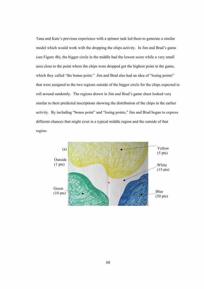
Figure 4. Student-generated games: (a) Kate and Tana’s game (b) Jim and Brad’s game. 69
Figure 5. The split-box for marble drops. 71 Figure 6. The Multi-level Split-box game board and the example of a counter. 75
Figure 7. Student-generated inscriptions for the rabbit hops in the pilot study. 79 Figure 8. The NetLogo interface: Hopping Rabbits Task. 82 Figure 9. The NetLogo interface: The Galton Box Task. 84 Figure 10. The figures (A, B, C, D, and E) shown in Pre-Interview Task 1:
Channels. 94 Figure 11. Alicia’s response in Pre-Interview Task 2: Ice-Cream. 100 Figure 12. Josh’s response in Pre-Interview Task 2: Ice-Cream. 101 Figure 13. Caleb’s response in Pre-Interview Task 2: Ice-Cream. 102 Figure 14. Emily’s response in Pre-Interview Task 2: Ice-Cream. 102 Figure 15. Maya’s response in Pre-Interview Task 2: Ice-Cream. 104 Figure 16. Maya’s response in Pre-Interview Task 5: Marbles. 109 Figure 17. Alicia’s and Emily’s ways to display various groups of leaves
under the tree. 117 Figure 18. Students’ predictions for the distribution of chips
(15” above the dot) in G 1. 123 Figure 19. The results of first dropping chips experiment
(15” above the ground) in G 2. 125
ix
Figure 20. The dart board discussed in Task 3. 132 Figure 21. Student-generated games: (a) Group 1’s game (b) Group 2’s game. 135 Figure 22. The Split-box used in the study. 138 Figure 23. The Multi-Level Split-Box game with the counter
[shown in the picture on the right] used in the study. 148 Figure 24. Josh’s drawing to show the symmetry and the number of ways
to get each outcome in the multi-level split-box task. 155 Figure 25. The Bears Task. 157 Figure 26. Students’ inscriptions for finding all possible ways to arrange
blue and red bears in Task 8 (Picture on the left by Group 1 and picture on the right by Group2). 157
Figure 27. Possible paths for five random rabbit-hops (Group 1). 166 Figure 28. Possible and impossible outcomes for five rabbit-hops (Group 2). 167 Figure 29. Students’ inscriptions for the simulation of the rabbit-hops in
Group 1. 169 Figure 30. Students’ inscriptions for the simulation of the rabbit-hops in
Group 2. 170 Figure 31. Student-generated inscriptions for figuring out the number of
different ways for each outcome after 10 hops. 172 Figure 32. List of all possible ways to get to each final location after five
hops (Group 2). 179 Figure 33. Caleb’s estimation of likelihoods of outcomes by fractions. 182 Figure 34. Josh’s quantification of outcomes when rolling two dice. 186 Figure 35. A simulation of five hops and ten hops for 10,000 rabbits. 189 Figure 36. The NetLogo Galton box model interface showing the “shade-path.” 191 Figure 37. Post-Interview Task 1: Channels. 197 Figure 38. Post-Interview Task 2: Ice-Cream. 202
Table 1. Characteristics of students’ explanations of natural distributions during the interviews in the pilot study. 62
Table 2. Students’ predictions for flipping a coin five times and the actual
outcomes in the pilot study. 76 Table 3. The list of combinations and permutations of Heads and Tails for
five hops and the final position after five hops. 80 Table 4. Synopsis of the sequence of tasks used in the teaching experiment
study. 89-90 Table 5. The summary of each participant’s responses and reasoning across
the pre-interview tasks. 115 Table 6. The specified rules for the designed games. 133 Table 7. Predictions and results for 10-individual marble drops in Group1. 139 Table 8. Group 1’s results and predictions in the multi-level split-box game. 149 Table 9. Group 2’s results and predictions in the multi-level split-box game. 152 Table 10. Group 1 student predictions for 5 individual coin-tosses and results. 160 Table 11. Group 2 student predictions for 5 individual coin-tosses and results. 161 Table 12. Students’ responses to the “Channels” task in pre- and
post-interviews (I = Incorrect, C = Correct). 201
xii
ABSTRACT OF THE DISSERTATION
Investigating Elementary School Students’ Reasoning about
Distributions in Various Chance Events
by
Sibel Kazak
Doctor of Philosophy in Education
Washington University in St Louis, 2006
Professor Jere Confrey, Chairperson
Data and chance are two related topics that deal with uncertainty, and statistics
and probability are the mathematical ways of dealing with these two ideas, respectively
(Moore, 1990). Unfortunately, existing literature reveals an artificial separation between
probability and data analysis in both research and instruction, which some researchers
(Shaughnessy, 2003; Steinbring, 1991) have already called attention to. In a response to
the calls from other researchers (e.g., Shaughnessy, 2003) and recommendations from the
National Council of Teachers of Mathematics (NCTM, 2000), this dissertation focused
on the notion of distribution as a conceptual link between data and chance.
The goal of this study was to characterize a conceptual corridor that contains
possible conceptual trajectories taken by students based on their conceptions of
probability and reasoning about distributions. A small-group teaching experiment was
conducted with six fourth graders to investigate students’ development of probability
concepts and reasoning about distributions in various chance events over the course of
seven weeks. Each student also participated in pre- and post-interviews to assess their
xiii
understandings of probability concepts and probabilistic reasoning. The retrospective
analysis of eleven teaching episodes focused on children’s engagement and spontaneous
understandings in the context of the tasks designed to support them.
This study details the landmark conceptions and obstacles students have and the
opportunities to support the development of probabilistic reasoning and understanding of
probability concepts, such as equiprobability, sample space, combinations and
permutations, the law of large numbers, empirical probability, and theoretical probability.
Consequently, the results of this study yielded two major findings. First, students’
qualitative reasoning about distributions involved the conceptions of groups and chunks,
middle clump, spread-out-ness, density, symmetry and skewness in shapes, and “easy to
get/hard to get” outcomes. Second, students’ quantitative reasoning arose from these
qualitative descriptions of distributions when they focused on different group patterns
and compared them to each other. In addition, this study showed that students tended to
rely on causal reasoning about distributions relevant to real life contexts. They also often
provided deterministic and mechanical explanations when investigating random events
generated by a physical apparatus.
1
CHAPTER 1
INTRODUCTION
Stochastic ideas and intuitions are widely used in almost every field of our lives,
e.g. in sciences, in games, in sports, and in legal cases, when we make decisions under
uncertainty. Particularly, probability plays a very important role in dealing with
uncertain events in many different ways, from predicting tomorrow’s weather to
supporting a conclusion by evidence. As people make decisions under the conditions of
uncertainty, the knowledge of probability and data analysis becomes of critical
importance for ordinary citizens to make judgments in chance situations as well as to
make decisions on the basis of numerical information in their lives.
Data and chance1 are two related topics that deal with uncertainty, and statistics
and probability are the mathematical ways of dealing with these two ideas, respectively
(Moore, 1990). When the National Council of Teachers of Mathematics (NCTM)
Curriculum and Evaluation Standards for School Mathematics (NCTM, 1989) publicly
strengthened their emphasis on these topics, probability and data analysis2 began to be
introduced in the school mathematics curriculum at all grade bands. After a decade, to
keep up with the rapid changes in the world and to make school mathematics
understandable and useable in everyday life situations for students, the NCTM released
Principle and Standards for School Mathematics (NCTM, 2000) emphasizing that a
mathematics curriculum should focus on important mathematics which is useful in a
variety of school, home, and work settings. Thus, data analysis and probability strand
1 Throughout the dissertation, the term “chance” is used to refer to a broader range of ideas and applications of probability while the term “probability” refers particularly to the formalizations involved in assigning probability values to the events (Konold, 2006, personal communication). 2 The term “data analysis” is used to refer to the mathematical content strand in the school curriculum that deals with the ideas of statistics.
2
have become one of the content standards students should learn from Pre-kindergarten
through Grade 12.
Unfortunately, existing literature reveals an artificial separation between
probability and data analysis in both research and instruction, which some researchers
(Shaughnessy, 2003; Steinbring, 1991) have already called attention to. It is true that
there is a body of research in statistics education that links data and chance in the context
of sampling, sampling distribution, and variation in various sampling tasks (e.g.,
& Moritz, 2000). However, this is because probability was foundational in developing
the ideas of sampling and sampling distribution and could not be eliminated. Because
these are treated as more advanced topics, students in K-12 are introduced to the statistics
and probability as isolated and relatively independent topics in mathematics instruction
and curriculum.
In the traditional approach, probability and data analysis are thought as very
separate topics. One teaches probability starting with the counting principles and
Kolmogorov’s axioms3 and maybe teaches with the frequentist approach4 in which
central tendency is discussed as a way of looking at data distribution that is simply a
display of the actual outcomes, rather than as probabilistic entities. In data analysis
instruction, one teaches about the ideas of center, spread, and shape of data which are not
necessarily probabilistic. This separation is also found in the elementary school
mathematics curriculum, where the tendency is to have emphasis on number concepts,
3 Axioms of probability: (1) Probability of an event is a number between 0 and 1. (2) The probability of an event that is the whole sample space is 1. (3) For any sequence of mutually exclusive events, the probability of at least one of these events occurring is just the sum of their respective probabilities. 4 An experimental approach to probability based in the limiting relative frequency of occurrences of an event in an infinite number of trials (Konold, 1991).
3
such as whole numbers, decimals, percents, fractions, and rational numbers, followed by
data collection and analysis, particularly the descriptive statistics concepts (i.e.,
minimum, maximum, range, mean, mode, and median) and the graphical representations
(i.e., line plots, tally charts, bar graphs, and line graphs). In this traditional approach, the
conceptual link between probability and data analysis is not treated until the discussion of
statistical inference (in advanced levels) in which the idea of probability is imposed.
My study challenges this traditional treatment of probability and data analysis
topics and examines the role of the notion of probability distribution as a way to integrate
these topics together in early grades. This idea builds on previously conducted studies
which reveal two treatments of distribution: (1) A view of data as aggregate within
statistical reasoning about distributions and comparing distributions in data analysis (e.g.,
Cobb, 1999; Lehrer & Schauble, 2000; Hancock, Kaput & Goldsmith, 1992); and (2) A
view of distribution across different outcomes as a sample space associated with
probabilities within probability distribution and probabilistic reasoning (e.g., Horvath &
Given the superficial division between the discussions of probability and data analysis in
the research and instruction discussed above, this study was conducted as an attempt to
understand the role of the notion of distribution as a link between the data and chance and
contribute to the existing literature by addressing the gap.
Through a small-group teaching experiment with fourth-grade students in which I
was the teacher-researcher, I investigated students’ reasoning about distributions in
various chance events supported by the design of a sequence of tasks. The focus of the
study is to examine individual students’ development through the teaching experiment as
they interacted with the teacher-researcher and the other students in their groups. The
open-ended tasks which were piloted prior to the study particularly focused on the
centered distributions. Students explored these distributions in a variety of ways, such as
using chance devices and conducting simulations of uncertain events that can be modeled
by a binomial probability distribution in a computer environment.
5
Given the focus of the study, the main research question that guides the
investigation of the fourth-grade students’ reasoning about distributions in chance events
is: How do students develop reasoning about distributions when engaging in explorations
of chance situations through a sequence of tasks, in which students were asked to provide
predictions and explanations during the experiments and simulations with objects,
physical apparatus, and computer environment?
Outline of Dissertation
The dissertation is organized into eight chapters. Chapter 1 introduces the study
through a brief overview. The problematic that set up the need for this study, the focus of
this study, and the research questions are presented in this chapter. Chapter 2 reviews the
literature that provided the framework for the study. The selected literature in the second
chapter focuses on the emergence of the probability concept; students’ misconceptions or
heuristics under uncertainty; students’ development of probability concepts; the models
of students’ probabilistic reasoning; and students’ reasoning about distributions in the
context of data analysis. Chapter 3 presents the theoretical framework and methodology
of the study with the description of the research design, the constructivist and socio-
cultural philosophies, the participants, the study instruments and tasks, the data gathering
process, and the method of analysis. Chapter 4 presents the pilot study results and the
revision of the tasks used in the teaching experiment study based on these results. Also,
it discusses the development of conjecture that guided the design study. Chapter 5
includes the analysis of the pre-interviews with each participant. Chapter 6 presents the
detailed description of students’ reasoning about distributions in chance events during the
6
teaching experiment sessions. Chapter 7 includes the analysis of the post-interviews with
each student. Finally, Chapter 8 discusses the findings of the design study based on the
research question. Also, it presents the limitations of the study, the implications for
research and practice, and for the future research.
7
CHAPTER 2
REVIEW OF LITERATURE
In this chapter, I begin to review relevant literature on probability that provided
the framework for my study. In reviewing the literature regarding the reasoning about
chance, it is necessary and helpful to consider the historical roots of the probability
concept before addressing the contributions of the empirical work in probability.
Afterward, I provide an overview of the selected research on different kinds of thinking
in the acquisition of probabilistic knowledge, students’ conceptions of probability, and
models of students’ probabilistic reasoning. Then, I present the body of research in data
analysis that discusses the notion of distribution in those studies. The chapter concludes
with the key aspects of the literature and with the statement of the purpose of this study.
Historical Roots of the Probability Concept
The early ideas of probability, chance, and randomness have existed since ancient
times. The use of astragali (a heel bone in animals) and then the early form of die and
drawing lots (e.g., straws of unequal length) in gaming, divination, and fortune telling are
indications of those ideas (David, 1962). However, the probability concept (as a
quantifiable means to describe likelihood) did not emerge until the mid 1600s (Hacking,
1975). The concept of probability itself has developed rather recently when the
probabilistic ideas were applied to make decisions in a variety of contexts including the
games of chance, law, and life insurance. Prior to this, the word probability was
associated with two important ideas, namely scientia (knowledge) and opinio (opinion)
(Hacking, 1975). While scientia refers to knowledge of universal truths as well as
8
demonstrable knowledge, in opinio probability means approvability of an opinion by
some authority or through God-given signs in nature.
A concept of evidence was key to the development of probability concept from
the medieval periods to the modern era. In his discussion of evidence, Hacking (1975)
distinguishes between two types of evidence: (1) external evidence, having to do with the
evidence of testimony, and (2) internal evidence, having to do with the evidence of
things. He notes some concepts of evidence that have been around during the
Renaissance. Those included the concept of testimony and authority “as the basis for the
old medieval kind of probability that was an attribute of opinion” (ibid, p. 32). However,
inductive (internal) evidence did not exist until the seventeenth century. The formation
of the inductive nature of the evidence evolved from the concept of sign as evidence in
opinio (Hacking, 1975). Prior to this transformation, the sign-as-evidence indicated with
the concept of probability regarded as a matter of testimony by some authority, such as
the church. Hacking noted the connection between sign and probability in a sense that
signs had probabilities considered more probable than another as they came from the
ultimate authority of nature. Moreover, probable signs through which nature gives
testimony encompass a spectrum of degrees of evidence from “imperfect” to “very often
right” and hence could be both suggestive (i.e., smoke and fire) and predictive (i.e.,
drawing lots and reading the future). This is to say, “on the one hand, a sign considered
as testimony made an opinion probable; on the other, the predictive value of a sign could
be measured by the frequency with which the prediction holds” (Hald, 2003, p. 31).
According to Hacking (1975), the emergence of the new concept of inductive evidence
(empirical evidence) thus resulted in the recognition of the connection between natural
9
signs (i.e., probability as testimony with the approval of data) and the frequency of their
correctness (i.e., probability as stable frequencies in repeated trials).
In relation to this transformation from the old concept of sign to the inductive
evidence, Hacking notes the duality of the concept of probability that emerged around
1660. More specifically, this dual property of probability, which still exists, is known as
(1) epistemic notion of probability, referring to support by evidence (i.e., since his
breathing had become shallow and some of his organs had begun to fail, the doctors say
he is close to death.) and (2) statistical notion of probability, concerning with stable
frequencies of occurrences or certain outcomes (i.e., the probability of getting heads
when you toss a coin repeatedly many times gets closer to 0.5). According to Hald
(2003), epistemic probabilities apply to “measuring the degree of belief in a proposition
warranted by evidence which need not be of a statistical nature” (p.28) while statistical
probabilities refer to “describing properties of random mechanisms or experiments, such
as games of chance, and for describing chance events in populations, such as the chance
of a male birth or the chance of dying at a certain age” (p. 28). Moreover, in Hald’s
characterization of these two notions of probability, subjective probabilities are related to
our imperfect knowledge or judgment whereas objective probabilities are based on
symmetry of games of chance, such as equally possible outcomes, or the stability of
relative frequencies in the long run.
An implication of the dual nature of probability mentioned above is twofold. On
the one hand, the epistemic or subjective notion of probability emphasizes personal
probability relative to our background knowledge and beliefs and, thus, enables us to
represent learning from experience (i.e., new evidence affect what we know and believe,
10
so we can represent our degrees of belief by coherent personal probabilities that satisfy
the basic rules of probability) (Hacking, 2001). On the other hand, the statistical or
objective notion of probability underlines stable and law-like regularities in relation to
physical and geometrical properties of chance setups and events by calculating relative
frequencies from experiments (Hacking, 2001).
According to Steinbring (1991), “beginning with very personal judgments about
the given random situation, comparing the empirical situation with their intended models
will hopefully lead to generalizations, more precise characterizations, and deeper
insights” (p.146). In other words, Steinbring suggested that subjective probabilities based
on our knowledge, but not simply a matter of opinion, could be checked by experiment.
This interpretation of subjective probabilities was similar to the use of the term
‘subjective’ among the physicists as well as in Jacques Bernoulli’s important distinction
between the subjective and objective probabilities which revolutionized the probability
theory (Hacking, 1975). In relation to this revolution, Hacking pointed out, the main
contribution of Bernoulli was his discussion and extension of the probability concept and
its applications in his book, Ars Conjectandi, published in 1713 (Hald, 2003). In
particular, Bernoulli distinguished between “the probabilities which can be calculated a
priori (deductively, from considerations of symmetry) and those which can be calculated
only a posteriori (inductively, from relative frequencies)” (Hald, 2003, p. 247).
Furthermore, in his book Bernoulli proved the first limit theorem of probability as an
attempt to show the applicability of the calculus of probability to other fields where
relative frequencies are used as estimates of probabilities. In doing so, he approached the
question of whether there was a theoretical counterpart (statistical model) to the empirical
11
outcomes (observations) (Hald, 2003). A formulation of Bernoulli’s theorem is the
following:
Consider n independent trials, each with probability p for the occurrence of a certain event, and let sn denote the number of successes. According to probability theory, sn is binomially distributed… [And] hn [hn=sn/n, the relative frequency] converges in probability to p for n → ∞. (Hald, 2003, p. 258)
The theorem basically says that as the number of trials gets larger, the difference between
the theoretical probability and the empirical result becomes smaller.
An educational analysis of the distinction between the subjective and objective
probabilities and its formulation in the Bernoulli’s theorem can provide a rich context to
discuss the probability and statistics with an emphasis on the conceptual link between
these two topics. For instance, the following model (Figure 1) depicts both the ideas
discussed in Hacking’s historical accounts for the emergence of the probability concept
and the implications of the Bernoulli’s Theorem (Kazak & Confrey, 2005).
Figure 1. A model to link the discussions of probability and statistics.
This model suggests that when we talk about probabilities, we draw upon a
variety of evidence, such as personal knowledge or belief, empirical results, and
Simulations Experiments
Empirical (Observations)
Opinio
Prediction/Evidence Subjective
Personal probabilities (In experience)
Objective
Theoretical probabilities
n → ∞ The Law of Large Numbers
Scientia
Theoretical (Statistical models)
Relative to our background knowledge or beliefs
Relative frequencies in relation to properties of chance setups and events by calculating relative frequencies from experiments
12
theoretical knowledge. It further suggests that as one learns to appeal to evidence and
create and run simulations, one begins to link opinio to scientia. Especially, young
students’ understandings of probability are based on their personal and experiential
knowledge about the world. Therefore, the idea of simulation of probability experiments
is key to this study as a way to link empirical results to theoretical outcomes. Also,
Bernoulli’s Theorem is a mediator between the empirical data and the theoretical
probabilities through the law of large numbers.
Different Kinds of Reasoning under Uncertainty
An extensive body of research has primarily identified and documented different
types of thinking when making inference or judgment about an uncertain event, which are
often called as misconceptions, heuristics, intuitions, or beliefs, across a wide range of
age groups from young children to college students. Those include the representativeness
heuristic, the availability heuristic, the outcome approach, the law of small numbers, the
illicit use of the proportional model, and the equiprobability bias (Van Dooren, De Bock,
each of these different ways of reasoning under uncertainty as they relate to my study.
13
Representativeness Heuristic
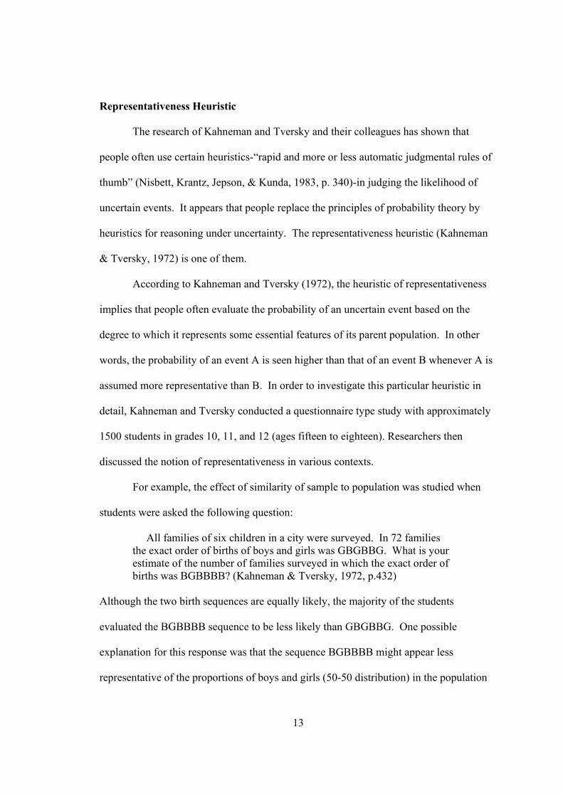
The research of Kahneman and Tversky and their colleagues has shown that
people often use certain heuristics-“rapid and more or less automatic judgmental rules of
thumb” (Nisbett, Krantz, Jepson, & Kunda, 1983, p. 340)-in judging the likelihood of
uncertain events. It appears that people replace the principles of probability theory by
heuristics for reasoning under uncertainty. The representativeness heuristic (Kahneman
& Tversky, 1972) is one of them.
According to Kahneman and Tversky (1972), the heuristic of representativeness
implies that people often evaluate the probability of an uncertain event based on the
degree to which it represents some essential features of its parent population. In other
words, the probability of an event A is seen higher than that of an event B whenever A is
assumed more representative than B. In order to investigate this particular heuristic in
detail, Kahneman and Tversky conducted a questionnaire type study with approximately
1500 students in grades 10, 11, and 12 (ages fifteen to eighteen). Researchers then
discussed the notion of representativeness in various contexts.
For example, the effect of similarity of sample to population was studied when
students were asked the following question:
All families of six children in a city were surveyed. In 72 families the exact order of births of boys and girls was GBGBBG. What is your estimate of the number of families surveyed in which the exact order of births was BGBBBB? (Kahneman & Tversky, 1972, p.432)
Although the two birth sequences are equally likely, the majority of the students
evaluated the BGBBBB sequence to be less likely than GBGBBG. One possible
explanation for this response was that the sequence BGBBBB might appear less
representative of the proportions of boys and girls (50-50 distribution) in the population
14
(Kahneman & Tversky, 1972). As a follow-up question, students were asked to estimate
the frequency of the sequence BBBGGG in the same context. Then, the student
responses showed that it was seen significantly less likely than GBBGBG. However, all
three sequences, certainly, are equally likely to occur based on the theoretical model of
assigning probabilities. Researchers then claimed that the sequence BBBGGG seemed to
the students less random in terms of irregularity in the sequence.
Kahneman and Tversky (1972) also examined the representativeness prediction
concerning the sample size conducting an additional experiment with 97 undergraduate
students with no background in statistics or probability. For instance, one of the problems
given to the students is the following:
A certain town is served by two hospitals. In the large hospital about 45 babies are born each day, and in the smaller hospital about 15 babies are born each day. As you know, about 50% of all babies are boys. The exact percentage of baby boys, however, varies from day to day. Sometimes it may be higher than 50%, sometimes lower. For a period of one year, each hospital recorded the days on which (more/less) than 60% of the babies born were boys. Which hospital do you think recorded more such days? (Kahneman & Tversky, 1972, p.443)
To control the response from being biased, the problem was given in two forms. While
half of the students were asked to evaluate whether an outcome that is more extreme than
the specified critical value is more likely to occur in a small or in large sample, the
remaining students judged whether an outcome that is less extreme than the specified
critical value is more likely to occur in a small or in large sample. Then, Kahneman and
Tversky found the following results:
15
More than 60 % (Form I) Less than 60% (Form II)
The larger hospital 12 9* The smaller hospital 10* 11 About the same 28 25
(The correct responses were stared.)
Normatively1, an extreme outcome is more likely to happen in a small sample.
Therefore, in form I, the correct answer is that the smaller hospital is more likely to have
the days on which more than 60% of the babies born were boys. In form II, on the other
hand, such an outcome is more likely to happen in a larger sample. However, more than
half of the participants in this study chose “about the same” in both forms. According to
Kahneman and Tversky, student responses showed no systematic preference for the
correct answer. Indeed, one can hardly explain the pattern in the student responses.
Moreover, in another study, a group of college students was given a slightly different
version of the problem in form I and majority of the students chose “no difference”
(equivalent to “about the same”) (Shaughnessy, 1977). When students were asked why
they chose that particular answer, Shaughnessy reported that students evaluated the
chance of getting a certain percent of boys as the same in any hospital, without any regard
to the sample sizes.
Availability Heuristic
The availability heuristic occurs when people evaluate the likelihood of events on
the basis of how easy to recall the particular instances of the event for them (Tversky &
Kahneman, 1973). In these cases, people’s predictions of the probabilities are often
1 In the literature, “normative” is used to refer some theoretical model for assigning probabilities or likelihoods to events.
16
mediated by an assessment of availability. For instance, one may assess car accident rate
in a particular location by recalling a car accident incidence he had in that location
previously. To investigate such systematic biases based on the reliance on the availability
heuristic, Tversky and Kahneman conducted a series of experimental studies in which
students judged the frequencies or the probabilities of the events.
In one study, Tversky and Kahneman (1973) explored the role of availability in
the evaluation of binomial distributions. The seventy-three 10th and 11th grade students
were given the following task:
Consider the following diagram: X X O X X X X X X X O X X O X X X X X X X O X X X X X X X O O X X X X X
A path in this diagram is any descending line which starts at the top row, ends at the bottom row, and passes through exactly one symbol (X or O) in each row. What do you think is the percentage of paths which contain
6-X and no-O ____% 5-X and 1-O ____% . . . No-X and 6-O ____%
Note that these include all possible path-types2 and hence your estimate should add to 100%. (Tversky & Kahneman, 1973, p. 216)
Tversky and Kahneman initially postulated that the students first glance at the diagram
and predict the relative frequency of each path-type on the basis of how easy it is to
construct individual paths of this type. Accordingly, students would erroneously evaluate
paths of 6 X’s and no O to be the most frequent since there were many more X’s than O’s
2 The actual distribution is binomial with p=5/6 and n=6 from a normative perspective.
17
in each row of the diagram. Indeed, of the 73 students, 54 responded that there were
more paths consisting of 6 X’s and no O than paths consisting of 5 Xs and 1 O. In
reality, however, the latter is more frequent. Hence, Tversky and Kahneman’s study
(more extensive than what is discussed here) suggests that people have a tendency to
make predictions based on how accessible instances of an event are to the memory, or on
the relative ease of constructing particular instances of the event.
Outcome Approach
Konold (1991) introduced another terminology “outcome approach” on which
many people make decisions about probability tasks. More specifically, Konold found
that outcome-oriented students do not perceive the results of a single trial of an
experiment as one of many such trials. As a result, they often simply employ the idea of
“anything can happen” when they believe that no predictions can be made about random
phenomena. Next, I briefly examine the outcome approach for making probability
judgments as it is discussed in Konold et al. (1993).
In one study Konold and his colleagues investigated students’ probabilistic
reasoning. In this study, the age and background of the subjects varied: 16 high school
students who were to attend a workshop as part of Summermath program, 25 volunteer
college students enrolled in a remedial-level mathematics course, and 47 undergraduate
students enrolled in a statistical methods course. As part of the questionnaire, students
were asked to choose from among possible sequences the “most likely” to result from
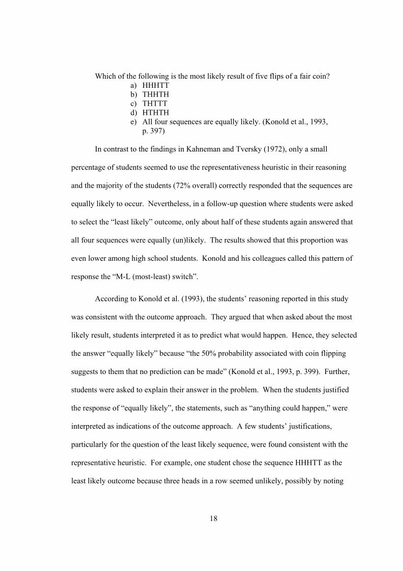
flipping a coin five times in the following task:
18
Which of the following is the most likely result of five flips of a fair coin? a) HHHTT b) THHTH c) THTTT d) HTHTH e) All four sequences are equally likely. (Konold et al., 1993,
p. 397)
In contrast to the findings in Kahneman and Tversky (1972), only a small
percentage of students seemed to use the representativeness heuristic in their reasoning
and the majority of the students (72% overall) correctly responded that the sequences are
equally likely to occur. Nevertheless, in a follow-up question where students were asked
to select the “least likely” outcome, only about half of these students again answered that
all four sequences were equally (un)likely. The results showed that this proportion was
even lower among high school students. Konold and his colleagues called this pattern of
response the “M-L (most-least) switch”.
According to Konold et al. (1993), the students’ reasoning reported in this study
was consistent with the outcome approach. They argued that when asked about the most
likely result, students interpreted it as to predict what would happen. Hence, they selected
the answer “equally likely” because “the 50% probability associated with coin flipping
suggests to them that no prediction can be made” (Konold et al., 1993, p. 399). Further,
students were asked to explain their answer in the problem. When the students justified
the response of “equally likely”, the statements, such as “anything could happen,” were
interpreted as indications of the outcome approach. A few students’ justifications,
particularly for the question of the least likely sequence, were found consistent with the
representative heuristic. For example, one student chose the sequence HHHTT as the
least likely outcome because three heads in a row seemed unlikely, possibly by noting
19
how well a sample represents the randomness of process that generates it. Thus, Konold
and his colleagues conjectured that the M-L switch stemmed from a change in
perspectives, from an outcome approach to the representativeness heuristic. However,
this inconsistency is probably not problematic to the students since they responded on the
basis of different frameworks.
Law of Small Numbers
The tendency to regard small samples as highly representative of the population
from which they are sampled and to use them as a basis for inference and generalizations
is a misapplication of the law of large numbers to small samples (Tversky & Kahneman,
1982). The belief in the law of small numbers causes someone to hold an unwarranted
confidence in the validity of conclusions based on small samples and to underestimate the
effect of sample size on sampling variability. Therefore, it hinders the idea that extreme
outcomes are more likely to occur in small samples.
Illicit Use of the Proportional Model
Van Dooren et al. (2003) provided an insight into the misconception concerning
the neglect of sample size reported by Fischbein and Schnarch (1997) when they
elaborated on the “illusion of linearity” referred by a tendency to apply linear or
proportional models improperly to any situation. For example, in Fischbein and
Schnarch (1997), students from different grades (5th through 11th) were given a
questionnaire consisting of some probability problems related to well-known
probabilistic misconceptions. One of the problems was as follows:
20
The likelihood of getting heads at least twice when tossing three coins is: smaller than
equal to greater than
the likelihood of getting heads at least 200 times out of 300 times. (ibid, p. 99)
According to the law of large numbers, as the sample size (or the number of trials)
increases, the relative frequencies tend to approach the theoretical probabilities.
However, the majority of the students in this study thought that the probabilities were
equal and the percentage of incorrect responses got higher as the age of the students
increased (from 30% of the fifth graders to 75% of the eleventh graders) . These students
reasoned that 2/3 = 200/300 and thus the probabilities were the same. In this particular
example, students did not pay attention to the role of sample size in calculating
probabilities. Instead, they overgeneralized the linear or proportional model in
comparing the probabilities of the two events. Hence, based on the findings of this
problem and its variants in other studies, Van Dooren et al. (2003) asserted that certain
systematic errors in probabilistic reasoning could be a result of an unwarranted
application of proportionality.
Equiprobability Bias
Lecoutre (1992) stated that people tend to view all possible outcomes of “purely
random” situations as equally likely. For instance, when two dice are simultaneously
rolled, what are the chances of obtaining a total of 9 vs. a total of 11? With regard to the
dice problem, Lecoutre and her colleagues observed the equiprobability bias in students’
responses. In particular, these students believed that it was equally likely to get 9 and 11
“because it is a matter of chance” (p. 561). In other words, they assume that any random
21
event is equiprobable by nature in association to the ideas of chance and luck. In the dice
problem, nevertheless, there is a greater chance to obtain 9 because there are twice as
many different ways to get it (i.e., 5 and 4, 4 and 5, 3 and 6, 6 and 3; vs. 5 and 6, 6 and 5).
Moreover, Pratt (2000) reported on Lecoutre’s equiprobability bias in his study
where a pair of students (10-year olds) assumed that the totals of two dice and of two
spinners with three equal parts each labeled 1, 2, and 3 would be uniformly distributed.
For example, students expected that all the totals for either two dice or two spinners were
equally easy or hard to obtain. One student reasoned that the chances of getting any total
were equally likely because each die was fair and the combinations of two dice must be
fair as well. Moreover, in making sense of two spinners, the other student stated that
there was a 50-50 chance of getting any total between 2 and 6. The misuse of the phrase
“50-50 chance” was also documented by Tarr (2002). In Tarr’s study, prior to
instruction, many fifth-grade students incorrectly applied the phrase “50-50 chance” to
(1) a situation in which all outcomes were equally likely to happen, such as a sample
space including one black marble, one blue marble, one red marble, and one yellow
marble in a jar, and (2) a sample space with two outcomes, such as one blue marble and
four yellow marbles in a jar.
It appears that students tend to overgeneralize the equiprobable assumption of
certain probability events, such as a six-sided die and a spinner with equal partitions,
which are commonly used in school or in games of chance, to situations that are non-
equiprobable. Even the phrase “50-50 chance” which is associated with equal chances
can be misapplied to situations when there are three or more equally likely outcomes and
there are only two outcomes, but which are not equally likely to occur.
22
Students’ Conceptions of Probability
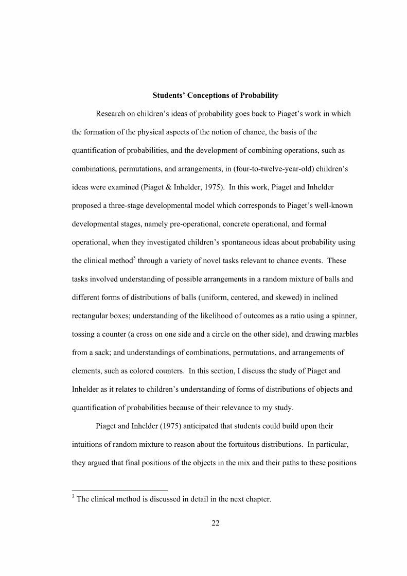
Research on children’s ideas of probability goes back to Piaget’s work in which
the formation of the physical aspects of the notion of chance, the basis of the
quantification of probabilities, and the development of combining operations, such as
combinations, permutations, and arrangements, in (four-to-twelve-year-old) children’s
ideas were examined (Piaget & Inhelder, 1975). In this work, Piaget and Inhelder
proposed a three-stage developmental model which corresponds to Piaget’s well-known
developmental stages, namely pre-operational, concrete operational, and formal
operational, when they investigated children’s spontaneous ideas about probability using
the clinical method3 through a variety of novel tasks relevant to chance events. These
tasks involved understanding of possible arrangements in a random mixture of balls and
different forms of distributions of balls (uniform, centered, and skewed) in inclined
rectangular boxes; understanding of the likelihood of outcomes as a ratio using a spinner,
tossing a counter (a cross on one side and a circle on the other side), and drawing marbles
from a sack; and understandings of combinations, permutations, and arrangements of
elements, such as colored counters. In this section, I discuss the study of Piaget and
Inhelder as it relates to children’s understanding of forms of distributions of objects and
quantification of probabilities because of their relevance to my study.
Piaget and Inhelder (1975) anticipated that students could build upon their
intuitions of random mixture to reason about the fortuitous distributions. In particular,
they argued that final positions of the objects in the mix and their paths to these positions
3 The clinical method is discussed in detail in the next chapter.
23
would form a certain distribution in which the form of the whole would be tied into the
notion of probability in children’s thinking. Then, Piaget and Inhelder conducted a study
with children of ages 4-12 to examine their understandings of uniform and centered
distributions. They used inclined boxes with a funnel-like opening in the middle of the
upper part of the box and equal-sized (2, 3, 4, or more) slots partitioned by a divider at
the bottom. Children were asked to make predictions and to do experiments by dropping
different numbers of balls from the funnel at the top of the box and then to explain the
arrangements of the balls into the slots at the bottom. According to Piaget and Inhelder,
in the first stage, young children (four to six years old) lacked an understanding of a
distribution of the whole as they failed to predict or generalize the symmetrical dispersion
of the balls in the slots. Although seven-to-ten-year-old children began to understand the
dispersion as a whole with more or less precise symmetry, they failed to recognize the
role of large numbers of balls in the second stage. For instance, there was a tendency to
think that a small asymmetry of the number of balls in the slots would increase, rather
than diminish, as more balls were dropped repeatedly. In the third stage, children (eleven
to twelve years old) began to quantify the distributions looking at the number of balls in
the slots, such as “just about equal-eight more” (p. 47). They also came to understand the
role of large numbers in the regularity of distributions, such as the fortuitous differences
diminish as the number of balls increases (a difference of 8 in 50 is bigger than 20 in 200
and 20-difference in 200 is bigger than 20 out of one thousand).
With regard to the quantification of probabilities, Piaget and Inhelder claimed that
children’s development of comparing the likelihoods of events depended on their ability
to relate the part (favorable outcomes) with the whole (all possible outcomes) and their
24
understandings of the outcome space and the combinatoric operations. For instance,
Piaget and Inhelder asked children which outcome would most likely to happen if they
were to draw all the marbles two at a time from a sack in which there were equal number
of blue and red marbles. In stage one, children tended to believe that picking the same-
color pairs (BB or RR) would be more likely than getting the mixed pairs (BR or RB) and
some did not even think of a possibility of a mixed pair. When children initially noticed
the possibility of the mixed case (RB or BR) in the second stage, they quickly responded
that the mixed pairs would come out more frequently than the pairs BB or RR, but failed
to quantify the frequency of the mixed outcomes. In stage three, children formulated
numerical quantification of possible outcomes (i.e., getting RB or BR is twice more likely
than getting either BB or RR) on the basis of their understandings of possible outcomes
and combinatoric reasoning skills.
In general, Piaget and Inhelder viewed the notion of ratio and proportion based on
the combinatoric operations (combinations, permutations, and arrangements) as the origin
of the development of chance. They also primarily focused on “the acquisition of a
complete (or more advanced) theoretical concept of chance by children” (Van Dooren, et
al., 2003, p. 116). However, there is another major contribution by Fischbein (1975) to
the research on the formation of the probability concept. According to Fischbein’s
perspective, intuitions that are global and immediate in nature are considered central to
the children’s development of the concept of probability and that these probabilistic
intuitions can be derived from the individual experiences as well as from the formal
education in school. Thus, Fischbein (1975) claimed that the development of conceptions
25
of probability could be mediated through instructional intervention and social
interactions.
To examine the role of intuitions in the development of probabilistic thinking,
Fischbein and his colleagues conducted a series of studies. In a relatively recent study,
Fischbein, Nello, and Marino (1991) investigated the origins and the nature of some
probabilistic intuitions regarding the types of events (i.e., impossible, possible, and
certain events), the roles of different embodiments of identical mathematical or stochastic
structure, and the compound events. The participants of this study included 211
elementary school students (ages of 9-11), 278 junior high school students (ages of 11-
14) without prior instruction on probability, and 130 junior high school students (ages of
11-14) with prior instruction in probability. In the usual classroom setting, the students
were asked to solve fourteen probability problems with an explanation.
Fischbein and his colleagues found that children did not necessarily have a
spontaneous understanding of the concepts “possible, impossible, and certain.” Some
students seemed to have difficulty in referring to certain events when they tended to
decompose the certain totality into a number of possibilities. For instance, a student
thought that obtaining a number smaller than 7 in rolling a die was “possible” because
one might get any number smaller than 7. Moreover, the concept of impossible seemed
to be identified with either “rare” (i.e., “It is impossible because the probability is very
small”) or “uncertain” (i.e., “It is impossible because one cannot be sure”).
In this study, students also were asked to compare two different situations with
the same mathematical (stochastic) structure, such as the probability of obtaining three 5s
either by rolling a die three times or by rolling three dice simultaneously. Fischbein et al.
26
found that the majority of the students recognized the equal probabilities as they got older
and received some instruction on probability. However, many students thought that there
was a higher chance of getting 5, 5, 5 by rolling a die three times because the process
could be better controlled to get the certain outcome, such as by using the same kind of
roll each time.
According to Fischbein et al. (1991), an intuitive understanding of the probability
of a compound event in relation to the magnitude of the sample space developed
spontaneously with age. For instance, in rolling two dice, the probability of getting the
sum of 3 is the same as the probability of obtaining the sum of 11 because 3 can be
obtained with rolling 5 and 6 or 6 and 5 and similarly one can get 11 by rolling 2 and 1 or
1 and 2 (hence there are two possible ways to get both sum). However, the researchers
pointed out several difficulties that conflicted with the correct evaluation of the
probabilities in compound events. Firstly, children did not have an intuition to consider
order of the outcomes, such as (5, 6) and (6, 5) in rolling two dice. Secondly, students
tended to disregard the specific limitation in the chance experiment. For example,
numbers like 8, 10, and so on, were also considered in two-dice game when students
listed the possibilities of getting the sum of 11. Thirdly, many students lacked a
systematic way for generating all possible outcomes related to a probability event.
Fourthly, due to the availability heuristic (discussed earlier in this chapter), students
tended to compare correctly the possibilities of getting 2 or 12 than obtaining 3 or 11
when rolling two dice (i.e., easier to identify 1+1 or 6+6 than 2+1 and 1+2 or 5+6 and
6+5). Finally, children and even adolescents seemed to estimate equal probabilities based
on the misunderstanding of the notion of chance. For example, students believed that any
27
two chance events had equal probabilities because the outcome depended only on chance
no matter what the given conditions were.
To summarize, for Piaget and Inhelder (1975), the development of probability
concept depended on children’s ability to recognize the relationship between the part and
the whole with regard to the outcomes of a random event, and their conceptions of
sample space, combinations, and permutations. For Fischbein and his colleagues
(Fischbein, 1975; Fischbein et al., 1991), children’s intuitions of probabilistic concepts
were of importance as their development into more formal concepts of probability could
be mediated through systematic instruction and experiences based on social interactions.
Next, I focus on a set of recent studies that documented a detailed model of students’
probabilistic reasoning by considering their performance along several aspects of
normative reasoning in stochastic theory (e.g., Horvath & Lehrer, 1998; Vahey, 1997;
and Vahey et al., 2000).
Models of Students’ Probabilistic Reasoning
Horvath and Lehrer (1998) identified five distinct, but related, components of the
classical model of probability that were used to investigate the understanding of chance
and uncertainty: (1) the distinction between certainty and uncertainty (predictable and
unpredictable nature of certain outcomes), (2) the nature of an experimental trial (one’s
determination of whether the probability events, such as two spins of a spinner, are
identical), (3) the relationship between individual outcomes and patterns of outcomes
(individual events may show unpredictable outcomes, whereas distributions of these
outcomes often yield predictable patterns), (4) the structure of events (how the sample
28
space relates to outcomes), and (5) the treatment of residuals (difference between
predicted and actual results). In the 2nd grade classroom study, students carried out
experiments with one or two 6-sided and 8-sided dice in pairs. They were asked to first
predict, then to generate results and to justify the relationship between expected and
obtained outcomes. They used bar graphs to record their results and sample spaces.
Next, I summarize the findings of Horvath and Lehrer (1998) in relation to the
components of the classical model of probabilistic reasoning listed above:
The distinction between certainty and uncertainty. Many children initially
assumed that rolling dice was not completely random. Until beginning to collect data
from dice rolling, they expected that they could predict the next outcome in rolling dice,
such as lucky numbers.
The nature of an experimental trial. Half of the students believed that the way of
tossing the dice will affect the outcome while the rest disagreed. The dispute was
resolved when they all agreed to roll dice out of a cup to ensure the uncertainty of
outcome.
The relationship between individual outcomes and patterns of outcomes. As they
had more experience with the tasks, most students believed that global patterns of events
were more predictable than local outcomes (any single outcome). They tended to make
predictions about the distribution of outcomes in long run, such as 50 trials, based on the
past results generated after 20 trials. Students’ reasoning about the predictability of the
distribution of outcomes and uncertainty of a single outcome was also affected by the
discussion of the sample space in this particular task. Students became highly confident
that they could predict the shape of the distribution of results rolling a die many times.
29
They, however, were not very convinced that they could predict the result of any single
roll. Moreover, the graphical representations highlighted the general shape of the
distribution and significance of results when students looked at the sample space graphs
(based on both combinations and permutations) and the actual outcome graph. It also
encouraged students to notice relationships at a global level (i.e. distributions) rather than
at a local level (i.e. comparing individual outcomes).
The structure of events. In discussing the relationship between the sample space
and outcomes, when generating all the possible ways to get the totals of rolling two eight-
sided dice, students debated over whether order was important (i.e., 1,5 and 5,1 are two
different ways for getting 6-permutations) or not. Some students argued that various
combinations, such as 1,5 and 5,1, were equivalent because of the commutative property
of addition (i.e., 1+5 = 5+1). Students’ understanding of the relationships between the
number of possible outcomes and the distribution of actual outcomes was quite weak.
When they made predictions about the distribution of results, only a few of them could
use the number of possible outcomes with no support of discussion and the bar graphs in
front of them.
The treatment of residuals. A few students came to understand residuals in terms
of the relationship between outcomes and the sample space, such as its overall
(triangular) shape based on the permutations for each outcome (see Figure 2). When the
results of the experiment (i.e., the frequency of each outcome after the experiment) did
not exactly match the predicted outcomes, students tended to reason by their lucky
numbers or by their past experiences with games involving dice. Moreover, after some
30
experiences with noticing residuals, most students seemed to make generalization based
on the previous results and change their predictions accordingly.
Figure 2. Graph for the sample space of the sum of two 6-sided dice.
Similarly, Vahey and his colleagues (Vahey, 1997; Vahey et al., 2000) noted four
aspects of normative reasoning in probability situations: (1) randomness (understanding
that the game is based on non-deterministic mechanism), (2) outcome space (enumerating
all possible outcomes), (3) probability distribution (probability of each outcome), and (4)
validity of evidence (the law of small or large numbers). Vahey and his colleagues
acknowledged the notion of fairness as a motivating and productive area of inquiry for
students investigating probability in computer-based activities. The researchers used the
four interrelated conceptual areas of probability theory to examine the seventh-grade
students’ probabilistic reasoning during their interactions with the Probability Inquiry
Environment (PIE), a collaborative, guided-inquiry learning environment, in which
students were asked to evaluate the fairness of games of chance.
In Vahey (1997), pairs of seventh-grade students were given tasks related to coin
flipping. For each game, students were asked to evaluate the fairness of the games based
31
on the information given in the PIE software interface including questions, a probability
tree (see Figure 3), and a bar chart, by predicting, playing, and interpreting the results. It
was found that initially students had different conceptions of fairness. Those included
equal chances of winning, some variation which is not systematically favorable to one
team, no cheating, and possibility to win for each team.
Figure 3. Probability trees for Two-Penny and Three-Penny games showing the possible outcomes for each team to win.
Vahey (1997) argued that a wide variety of ideas students had, either consistent or
conflicted with the normative reasoning, made it difficult to characterize students’
reasoning only on specific misconceptions. Therefore, the researchers considered ways
of eliciting students’ different ideas based on the four aspects of the normative reasoning
in probability:
The randomness. Students believed that the outcomes of coin flip were non-
deterministic. Their explanations differed though. While some students stated a notion
of randomness as being based on “luck and chance,” or that the results between trials
32
might vary, some of them viewed randomness as nothing could be predicted about future
events or anything could happen (i.e., Konold’s outcome approach).
The outcome space and the probability distribution. Students had difficulty in
making a distinction between the individual outcomes and the combination of all
outcomes that could score a point for a team. For instance, they reasoned that it was
easier to get HHT than getting HHH because there are more HHT. Moreover, one
student believed that some outcomes, like TTT or THT, were less likely to occur since it
was “too much of a pattern” (Vahey, 1997, p. 11). Vahey argued that students would
often switch between talking about the number of possible outcomes for each team to win
and the probabilities of outcomes. Like in Horvath and Lehrer (1998), students rarely
made reference to the outcome (or sample) space on their reasoning.
The validity of evidence. Students’ belief on the law of small numbers appeared in
two different ways. In the data-driven case, students tended to give up their theory based
on small number of trials (i.e., 10 or less), or not to generate a theory in the absence of
data. In the theory-driven case, students seemed not to accept data as relevant when the
data were in conflict with their theory.
Reasoning about Distributions in Data Analysis
A number of researchers focused on the notion of distribution as a big idea in
statistics and examined students’ reasoning about distributions within statistical reasoning
and modeling data. For example, Cobb and his colleagues (Cobb, 1999) approached
statistical reasoning in such a way that seventh-grade students were able to reason about
distributions with strong connections among various statistical topics, including the
33
statistical measures and the representations. These researchers believed that students
could develop their own understanding of central statistical ideas and topics as they
engaged with data analysis through statistical reasoning. For instance, when students
described given a set of data in terms of its qualitative features, the students began to
reason using trends and patterns from the context of the problem.
Cobb and his colleagues also focused on distributions in order to bring the topics,
such as mean, median, mode, spread-out-ness, and graphical inscriptions, together so that
students could develop understandings of these topics either by organizing distribution or
describing its characteristics through statistical reasoning. Therefore, they designed data
sets for analyses in which students could make decisions in the context of a real-life
problem situation. Moreover, students were encouraged to justify their reasoning in the
whole-class discussions to develop their own statistical understandings through these
tasks.
In their approach, Cobb and his colleagues (Cobb, 1999) pointed out that
students’ understanding of the distribution would be essential to reason about data as
aggregates. It was argued that students should think about data sets as entities that are
distributed within a space of possible values rather than as a collection of individual data
points (McClain et al., 2000). Therefore, the researchers emphasized the exploration of
qualitative characteristics of collections of data points (Cobb, 1999). Moreover, these
characteristics were treated as features of the situation from which the data were
generated. Thus, it was necessary to investigate how students understood the aspects of
distributions and how they interpreted a distribution as they reasoned statistically.
34
Since a graphical representation of the data was visual, the shape of the data
initially helped students to understand and interpret the given data in a context. Students
began to use informal language to describe the shape of the distribution. For example,
such words as clumps, clusters, bumps, gaps, holes, spread out, and bunched together,
were used to describe where most of the data were, where there were no data, and where
there were isolated pieces or natural subgroups of data. The researchers found that this
was an important step toward exploring the qualitative characteristics of a distribution.
Lehrer and Schauble (2000) were specifically interested in fostering the
emergence of model-based reasoning in mathematics and science in the context of data
investigation in the elementary grades (1st-5th). The researchers have seen the data
modeling as an important resource for exploring the world. In their work, data modeling
served “as part of a chain of inquiry, encompassing question-posing, the construction of
attributes, and the creation of structures and displays that function to aggregate attributes
over multiple cases” (p. 130). Similar to Cobb and others’ study (Cobb, 1999), Lehrer
and Schauble heavily relied on reasoning about aggregates (e.g. distributions) and
acknowledged that this form of reasoning appeared to be mastered over an extended
period of time and depended on thoughtful instructional support and opportunities for
practice. The analysis of classroom episodes (Lehrer & Schauble, 2000) suggested that
older students were able to consider the properties of distributions, such as measures of
center and dispersion. Accordingly, these students used them as resources to investigate
problems that required simultaneous consideration of center and variability.
35
Key Aspects of Literature
In this chapter, I discussed the existing knowledge base regarding the reasoning
about chance and data that formed a basis upon which this study was conducted. In this
section, I describe the key aspects of the existing literature that I used to frame my study
of fourth-grade students’ reasoning about distributions in chance events.
Firstly, the historical development of the probability concept provides insights
into the different interpretations of probability. Earlier in this chapter, it was discussed
that the distinction between the scientia (knowledge demonstrated deductively from first
principles) and the opinio (beliefs testified by some authority or through God-given
signs), and the transformation of what constituted acceptable evidence gave rise to the
dual meaning of probability. Hence, the concept of probability was historically used to
both describe the degrees of belief relative to our background knowledge (the epistemic
notion) and refer to the tendency of certain random events, such as flipping a coin, to
generate the stable regularities concerning the physical and geometric properties of the
chance event by computing the relative frequencies in the long run (the statistical notion).
This duality in effect recognizes both formal and informal uses of probability that can be
encountered in children’s reasoning about uncertain events. Also, it is of importance to
note the different views of probability, such as the classical, frequentist, and subjective,
that can be used to recognize various beliefs about probability held by students. More
specifically, the classical probability refers to the ratio of the number of favorable cases
in an event to the total number of equally likely cases. Then, the frequentist probability
of an event is defined as the limit of its relative frequency in a large number of trials.
Lastly, the subjective probability is considered as the degree of belief, like the opinio.
36
Several studies documented persistent erroneous conceptions (or misconceptions)
and strategies students held and employed in judging the likelihood of uncertain events.
Those included the representativeness and availability heuristics, the outcome approach,
the law of small numbers, the illicit use of the proportional model, and the
equiprobability bias. These misconceptions and errors in probabilistic reasoning is of
interest to this study because students come to the classroom with prior conceptions and
beliefs about physical, deterministic, and probabilistic phenomena based on personal
experiences and thus they may fall prey to some of these misconceptions. Accordingly,
young students may have difficulties in building intuitions for probability in chance
events and developing the normative probabilistic reasoning.
Moreover, the work on children’s spontaneous development of probability
concepts, including the formation of the physical aspect of chance, the role of large
numbers, the basis of quantifying probability, and the development of combinatoric
operations, and the studies on children’s probabilistic intuitions provided a foundation for
formulating a conceptual trajectory in this study. The research suggests that children’s
ideas of probability concept develop in relation to the formation of ratio and proportional
reasoning, and combinatoric operations. In addition, children’s intuitive understanding of
probability can be mediated through instruction before they develop strong
understandings of part-whole and combinatoric skills.
Characterizing students’ probabilistic reasoning only on particular misconceptions
does not provide a complete explanation of a variety of ideas students already possess.
Thus, some researchers considered several aspects of normative stochastic reasoning in
documenting the models of students’ reasoning. For example, they identified
37
randomness, the distinction between certainty and uncertainty, the nature of the
experimental trials, outcome space and probability distribution, the relationship between
individual outcomes and patterns of outcomes, the treatment of difference between the
expected and actual outcomes, and the validity of evidence as the characteristics of
probabilistic reasoning. Then, the students’ intuitive reasoning was compared to the
normative reasoning along these aspects. A variety of students’ ideas elicited through
this framework guided this study in determining what probability concepts to focus on,
how to structure and sequence the tasks, and how to analyze and interpret students’
spontaneous probabilistic understanding and reasoning.
Finally, the research on students’ reasoning about distributions in data analysis
provided the foundation of the focus of the study on the distributions in chance events.
Therefore, in this study, the notion of distribution as the aggregates of data is
emphasized. Moreover, students’ informal understandings of the qualitative aspects of
distribution in relation to the middle, spread or variability, and shape were of interest to
this study as these conceptions can be developed into more formal understanding of
distribution in chance events, such as the quantification of the most likely and the least
likely outcomes.
Purpose and Research Questions
As discussed above, the review of the literature provides a knowledge base on
students’ ideas about probability in a variety of ways. Moreover, the research on
students’ statistical reasoning about distributions in data analysis (e.g., Cobb, 1999;
Lehrer & Schauble, 2000) led me to consider the notion of distribution in the context of
38
chance in bringing the discussions of probability related topics together (i.e., sample
space4, combinations, permutations, probability, the law of large numbers,
representations, and inscriptions etc.). I also sought to understand the role of the notion
of distribution as a link between data and chance which is apparently absent in the
discussions of probability and statistics in research and instruction. Hence, the purpose
of this design study was to characterize a conceptual corridor that contains the conceptual
trajectories taken by the fourth-grade students based on their conceptions of probability
and reasoning about distributions in chance events by the design of a sequence of tasks.
Consequently, as stated in Chapter 1, the main research question was:
• How do students develop reasoning about distributions when engaging in
explorations of chance situations through a sequence of tasks, in which
students were asked to provide predictions and explanations during the
experiments and simulations with objects, physical apparatus, and computer
environment?
To understand this larger question, I developed four supporting research questions based
on the review of the literature:
• What are the students’ prior knowledge about probability concepts and
probabilistic reasoning?
• What kinds of informal knowledge and strategies can serve as starting points?
• What are the conceptual trajectories that students take during the teaching
experiment?
4 See the definitions of these terms in Appendix E.
39
• What are the resources (learned ideas) that students bring into the
understanding of probabilistic concepts and reasoning?
40
CHAPTER 3
THEORY AND METHODOLOGY
The review of literature in the previous chapter outlines the knowledge bases for
students’ ideas about chance and their reasoning under uncertainty. Methodologically,
many of these studies (e.g., Fischbein & Schnarch, 1997; Kahneman & Tversky, 1972;
Lecoutre, 1992) used questionnaires to assess students’ understanding and reasoning. In
particular, many of the tasks involved multiple-choice items. Although student responses
to the specific survey items in these studies permitted researchers to identify various
misconceptions, I agreed with Shaughnessy (1992) that clinical methodologies, such as
clinical interviews and teaching experiments, provide an opportunity to elicit a wider
variety of student ideas concerning stochastic tasks. Therefore, in this study, I conducted
pre-and post-clinical interviews and a small-group design experiment to examine
students’ understandings of probability and their reasoning about distributions in the
probability situations.
In designing the study and creating the tasks, I have mainly built from the
constructivist and the socio-cultural traditions which are discussed next. In the
subsequent sections, I describe the design of the study, the participants, the pilot study,
the study instruments and tasks, the methods of data collection, and the data analysis
procedures.
Theoretical Framework
This study employs a small-group design experiment model. According to Cobb,
Confrey, diSessa, Lehrer, and Shauble (2002),
41
Prototypically, design experiments entail both “engineering” particular forms of learning and systematically studying those forms of learning within the context defined by the means of supporting them. This designed context is subject to test and revision, and successive iterations that result play a role similar to that of systematic variation in experiment. (p. 9)
In particular, this study aims to investigate students’ reasoning about distributions in
chance events within tasks designed to support the development of students’ thinking.
Moreover, design experiments involve identifying “conjectured starting points, elements
of a trajectory, and prospective end points” as well as generating “stable conjectures
about both significant shifts in student reasoning and the specific means of supporting
those shifts” (ibid, p. 11) (see also Confrey & Lachance, 2000). The main focus of
design experiments, in particular one-on-one and classroom teaching experiments, is to
develop theories of the learning of individual students or of a classroom community, and
ways of supporting their learning of domain specific content. The study of intellectual
development of children can be a major source to generate those theories.
In the chapter tracing the historical development of design experiments, Confrey
(2006) argues that the purpose of a design experiment is to articulate two related ideas,
namely a conceptual trajectory and a conceptual corridor. In the context of a design
experiment, a conceptual trajectory is a possible pathway that students can navigate
during any particular set of instructional episodes and a conceptual corridor is a broader
concept that refers to all likely conceptual trajectories (Confrey, 2006). According to
Confrey, in constructing the conceptual corridor, one needs to start with students’ prior
knowledge and an initial problematic (the use of the term “problematic” in Confrey
(1998) refers to students’ interpretation of the problem in relation to his or her purposes,
goals, expectations, and prior knowledge). Moreover, the borders of the corridor are
42
determined by the design of a sequence of tasks. Confrey (2006) also defines landmarks
within the corridor, which are student conceptions that can be anticipated initially and
identified based on student responses and formative assessments. Furthermore, it is noted
that the specification of such a conceptual corridor should be flexible enough for students
to progress through that space.
The teaching experiment in the current study considered students’ conceptions
and reasoning, and some tools to support their development along possible conceptual
trajectories in a conceptual corridor. In doing so, the work of two theorists, Jean Piaget
and Lev Vygotsky, is of particular importance because of their contributions to the study
of children’s thinking and reasoning in mathematics and science education. Next, I will
present two major traditions, constructivist and socio-cultural perspectives, that are drawn
upon the theories of these scholars in mathematics education research. Also, the
methodological implications from these perspectives will be discussed.
Constructivism
The Relation between Knowledge and Reality in Constructivism
According to the constructivist view--an interpretation of Piaget--children’s minds
are not blank slates. Rather, students’ alternative conceptions must be taken into account,
using significant discussions and interactions around their various strategies (Confrey,
1994). Glasersfeld (1995) stated the two basic principles of constructivism: (1)
“Knowledge is not passively received but built up by the cognizing subject” and (2) “The
function of cognition is adaptive and serves the organization of the experiential world,
not the discovery of ontological reality” (p.18). While Glasersfeld called a stance that
43
accepts only the first principle “trivial constructivism”, he called a stance that accepts
both principles simultaneously “radical constructivism.” Hence, radical constructivism1
suggests that the individual builds up the knowledge, rather than passively acquires it.
Moreover, in the radical constructivist view, the relation of reality and knowledge is seen
as “an adaptation in the functional sense,” which refers to organization of our knowledge
of the world constituted by our perceptions and experiences, rather than “a more or less
picture-like correspondence or match” (Glasersfeld, 1984, p. 20).
Further, from a constructivist perspective, we do not have access to an objective
reality, in the sense that there is a reality independent of our way of knowing (Simon,
1995). Hence, Simon notes that we can never know whether a concept matches an
objective reality. In relation to the notion of fit (rather than match) Glasersfeld (1995)
used the concept of viability to indicate whether something fits in our experiential world
saying that “actions, concepts, and conceptual operations are viable if they fit the
purposive or descriptive contexts in which we use them” (p.14).
The Construction of Knowledge and Piaget’s Scheme Theory
In his book Genetic Epistemology (1970), Piaget explained knowledge
construction, particularly in relation to the logical and mathematical knowledge. He said
that knowing something does not mean copying it; rather it means acting upon it. Piaget
distinguished physical and logical mathematical knowledge. While the former refers to
the knowledge based on experiences in general, the latter applies to structures that are
abstract. According to Piaget, there are two types of abstraction: 1) simple abstraction
1 Through out this paper, “constructivism” will refer to “radical constructivism” as described by Glasersfeld here.
44
which is derived from the object that we act upon, and 2) reflective abstraction which is
drawn from the action itself. The second one is reflective in a sense that “at the level of
thought a reorganization takes place” (ibid, p. 18). Furthermore, reflective abstraction
always involves coordinated actions in mental processes.
Piaget (1970) considered coordinated actions as the basis of logical mathematical
thoughts. For him, coordinated actions become mental operations and a system of these
operations constitute a structure. Piaget’s notion of scheme refers to “whatever is
repeatable and generalizable in an action” (ibid, p. 42). Hence, scheme theory functions
to explain the stability and predictability of actions (Confrey, 1994). To interpret
Piaget’s scheme theory, one needs to understand two fundamental processes: assimilation
and accommodation. According to Piaget, assimilation involves an incorporation of new
experiences and perceptions of the world to the existing schema whereas accommodation
refers to adaptation of the existing schema to a new structure. Moreover, these two
processes work in a dialectical relationship. When a scheme leads to a perturbation, the
problematic will be called to action. Then, accommodation takes place in order to
maintain or reestablish the equilibrium.
Socio-cultural Perspectives
The Three Themes in Vygotsky’s Theoretical Framework
A socio-cultural approach to intellectual development in Vygotsky’s work is
based in the assumption that human action is mediated and it can never be separated from
its specific socio-cultural context (Werstch, 1991). In Wertsch’s interpretation of
Vygotsky’s theoretical approach, there are three fundamental themes (Werscth, 1985):
45
(1) The genetic, or developmental, analysis: The claim is that human mental
functioning can be understood only if we understand how and where the development has
occurred. Therefore, Vygotsky’s genetic analysis involves investigating the origins of
the mental processes and the ways that they are carried out.
(2) The social origins of higher mental functioning in the individual: For
Vygotsky, higher mental functioning in the individual emerges from the social context.
Thus, the direction of intellectual development is from social to individual. This idea is
stated in Vygotsky’s general genetic law of cultural development. According to this law,
there are two planes, social and psychological, on which the child’s cultural development
appears. More specifically, any mental function occurs first in the social plane (between
individuals as an interpsychological category) and then in the psychological plane (within
the individual as an intrapsychological category).
(3) The semiotic analysis: Vygotsky argued that higher mental processes are
mediated by tools2 and signs3. Development takes place when these different forms of
mediation create a transformation in mental functioning. In a Vygotskian approach,
mediational means are essentially social, not individual. They are the products of
sociocultural history, rather than inventions of each individual or discoveries of the
individual’s independent interaction with nature. Moreover, individuals have access to
the mediational means as part of a socio-cultural context, from which individuals
“appropriate4” them. For Vygotsky, the mediational means play an important role in
influencing others, and only later function to influence the individual.
2“ Tools” here refers to technical tools, such as a calculator, a graphic paper, etc. 3 “Signs” here refers to psychological tools, such as language, algebraic symbols, and so on. 4 Wertsch (1985) notes that this term comes from the later work of A. N. Leont’ev (1959).
46
The Concepts of Internalization and the Zone of Proximal Development
According to Vygotsky, there is an inherent connection between the
interpsychological plane and the intrapsychological plane. He was particularly concerned
with the processes in which mental functions are transformed from an external plane to
an internal plane. Since Vygotsky viewed higher mental functions as social processes,
for him the notion of internalization developed as “a process involved in the
transformation of social phenomena into psychological phenomena” (Wertsch, 1985, p.
63). While the external processes are necessarily socially interactional, internal processes
reflect certain aspects of this social interaction. Indeed, the higher mental functions
derive from the mastery of external sign forms. Wertsch also pointed out that for
Vygotsky, internalization is not a process of copying external reality on a preexisting
internal plane; instead, it is the process by which the internal plane is formed.
Vygotsky further described his concrete ideas about the connection between
interpsychological and intrapsychological functioning in relation to the concept of the
zone of proximal development (ZPD) (Wertsch, 1985). In an attempt to explain how to
evaluate interpsychological processes and relate them to their intrapsychological
outcomes, Vygotsky introduced the notion of the ZPD (Vygotsky, 1978):
[The ZPD] is the difference between [a child’s] actual development level as determined by independent problem solving and the level of potential development as determined through problem solving under adult guidance or in collaboration with more capable peers. (p. 86) The practical implications of this concept are of importance. Vygotsky argued
that intellectual development occurs within the ZPD of the child. He pointed out that
“learning which is oriented toward developmental levels that have already been reached
is ineffective from the view point of the child's overall development. It does not aim for
47
a new stage of the developmental process but rather lags behind this process" (ibid, p.
89). From this point of view, instruction should aim at a developmental level that is just
above the student's current developmental level. Moreover, in his formulation of the
ZPD, Vygotsky pointed to the role of imitation in learning. He argued that “children can
imitate a variety of actions that go well beyond the limits of their own capacities. Using
imitation, children are capable of doing much more in collective activity or under the
guidance of adults” (ibid, p. 88). For Vygotsky, with assistance of an adult or a more
capable peer every child can do more than he/she can by him/herself.
Methodological Implications
In order to link these philosophical traditions together, I have conducted a design
study situated in a constructivist tradition informed by a socio-cultural perspective
(Confrey & Kazak, 2006). Drawing on the work of Confrey (2006), one can link the
work of constructivism and socio-cultural perspectives into an approach that seeks to
document the development in student thinking about the relationships of probability and
data analysis.
From a constructivist position, it is essential to use methods that attempt to
describe the distinctive nature of the child’s thought. The two common methods that
have been widely used by constructivist researchers in mathematics education to explore
the thought processes of students are Piaget’s clinical method and the teaching
experiment method. Hence, I used the clinical method to interview individual students
before and after the study, and conducted a small-group teaching experiment to
investigate students’ probabilistic reasoning about distributions. In socio-cultural
48
research, Vygotsky’s work provides insightful ideas about intellectual development, and
yet the methodological implications of these ideas for empirical research are not often
clear (Wertsch & Kazak, in preparation). Therefore, I discuss next only the methods that
have roots in constructivism, and then I incorporate Vygotsky’s ideas into my discussion
of the design study in the data analysis section.
Clinical Method
The clinical method (or the clinical interview) originates with Piaget’s earlier
investigations of reasoning in children. In the method of clinical examination, Piaget
(1976) combined the method of standardized testing and natural observation without
falling into the pitfalls of these methods, by allowing the child to express his/her thoughts
and observing the child’s spontaneous behaviors or interactions. In Piaget’s clinical
method, the experimental aspect of the examination involves setting up a problem,
making hypotheses, adapting the conditions to them, and controlling each hypothesis by
testing it against the reactions that the interviewer stimulates in conversation. The
clinical examination is also dependent on direct observation, which allows the researcher
to capture the whole of the mental context.
Opper (1977) described the clinical method as “a diagnostic tool applied to
reasoning in children. It takes the form of a dialogue or conversation held in an
individual session between an adult, the interviewer, and a child, the subject of study” (p.
92). At the core of the clinical method is the hypothesis-testing feature of the method,
which allows the interviewer to draw inferences about the child’s thinking process by
observing his or her performance on certain tasks during the interview session. In
49
Piagetian studies, for example, the child is presented an experiment that involves both “a
concrete situation with objects placed in front of the child and a verbally presented
problem related to this situation” (ibid., p. 92). The interviewer has initial guiding
hypotheses to start with about the types of thinking that the child will engage in through
the given tasks in which physical or spatial manipulations are acted upon the materials.
In these tasks, the child is asked to provide predictions, observations, and explanations
for the results of the manipulations performed on the concrete objects. On the basis of
these verbal responses and actions, the interviewer tests his or her initial hypotheses.
Probing questions also further clarifies these responses. Reformulation of the original
hypotheses, if needed, and the formation of new hypotheses occur until the interviewer is
satisfied with the exploration of the child’s thinking as far as possible.
The description of the clinical method given above indicates that the interviewer
has complete freedom in conducting the interviews, such as the choice of the ways to
study the concept of interest and the flexibility to modify the experimental situation for
each particular child (Opper, 1977). In practice, however, Opper argued that a systematic
approach to conducting interviews would be needed for comparable results. Thus, a
partially standardized version of this method is commonly used in research based in the
Piagetian tradition. More specifically, a standard task with certain identical
manipulations is presented to each participant. In relation to the task at hand, all
participants are asked a number of identical questions. At the same time, the interviewer
has the freedom of rephrasing the questions according to the child’s responses and
following up the child’s novel responses and actions with additional questions or items in
order to understand better the child’s thinking and reasoning. Therefore, this partially
50
standardized version of the clinical method is “an attempt to combine the more structured
approach of standardized testing with the flexibility of the clinical method” (ibid., p. 95).
The Constructivist Teaching Experiment
The constructivist teaching experiment methodology is designed to investigate
students’ mathematics (which refers to children’s mathematical knowledge), and
mathematics of students (which represents the researcher’s interpretations or models of
students’ mathematics) in the context of mathematics teaching (Steffe & Thompson,
2000). Steffe and Thompson use of the phrase “students’ mathematics” is based on the
assumption of students’ mathematical reality as being different from the researcher’s
mathematical reality. Therefore, a goal of the researcher in a teaching experiment is to
construct models of students’ mathematics. The legitimacy of these models depends on
the extent to which the researcher can find rational grounds for students’ language and
actions.
To this end, the exploratory framework of the teaching experiment that is drawn
from Piaget’s clinical method involves basically “formulating and testing hypotheses
about various aspects of the child’s goal-directed mathematical activity in order to learn
what the child’s mathematical knowledge might be like” (Steffe, 1991, pp. 177). During
the teaching episodes, and between the teaching episodes as well, the teacher-researcher
both generates and tests hypotheses about possible meanings of the students’
mathematical language and actions. However, Steffe argues that the teaching experiment
is more than a clinical interview, because developing ways and means of influencing
students’ knowledge is part of the experiment. Hence, in this section I will primarily
51
focus on these distinct features of the teaching experiment methodology in mathematics
education.
The researcher’s role as teacher is a distinguishing characteristic of this method
(Steffe, 1991). Beyond acting as teacher, the teacher-researcher also attempts to
understand students’ mathematics in their ways and means of thinking and reasoning. In
doing so, the teacher-researcher creates situations and ways of interacting with the
students that foster students’ learning. More specifically, learning occurs as a result of
students’ interactions in particular situations that help students alter their current
schemes. The researcher is interested in the assimilating schemes of students in these
situations, situations which ought to be “interesting and challenging for students” (Steffe
& Thompson, 2000, p. 289). According to Steffe and Thompson (2000), deliberate
variation in the situations with respect to their context, material, and scope is an
important part of the framework of the teaching experiment. In doing so, however, the
teacher-researcher should not go so far beyond students’ current schemes that it requires
students to make major accommodations in their schemes. Rather, in fostering
accommodation, the teacher-researcher generates situations of learning from which a
perturbation results, so that students experience a moderate reorganization of their
existing schemes, for example by using them in novel ways.
52
Design of the Study
In order to answer the research questions set forth in Chapter 2, the work of Piaget
and Vygotsky and the methodological implications discussed above convinced me to
choose a design in which I could define a conceptual corridor of possible opportunities,
landmark conceptions, and obstacles. To do so, a sequence of tasks, some of which were
adapted from other studies, was developed based on my initial conjecture about linking
the discussions of probability and data analysis through the notion of probability
distribution, in light of the existing literature on students’ understanding of chance and
data, the historical development of the probability concept, and my mathematical content
knowledge about probability and statistics. Then, a pilot study was conducted to field
test the tasks developed for use in the teaching episodes. From the pilot study data,
conjectures about a conceptual corridor were also developed. Based on the concepts,
tools, and ideas relevant to the initial conjectures, the interview questions were selected
from the literature and from the National Assessment of Educational Progress (NAEP)
items (see Appendix A). Follow-up probes were used during particular encounters in the
interview tasks. The individual interview sessions took place several days before and
after the teaching sessions, to examine individual participants’ understanding of
probability concepts and their probabilistic reasoning. The teaching sessions were
conducted over a period of seven weeks in which participants in groups of three
completed the tasks designed for this study.
53
Participants
The participants were six volunteered fourth-grade students (9-year olds), three
boys and three girls (Alex, Alicia, Caleb, Emily, Josh, and Maya; all names are
pseudonyms). The sample was selected as a convenience sample. The participating
students were recruited through their classroom teacher at a local elementary school at
the beginning of the fall of 2005. The same teacher also helped me to recruit students
from her class for my pilot study in the spring of 2005. During the study, the interview
and teaching experiment sessions occurred in a room (previously used for Spanish lab) at
the school during the mathematics class period.
Pilot Study
In the spring of 2005, a pilot study was conducted to refine the tasks to be used in
the actual study and to develop initial conjectures about the conceptual corridor (see the
detailed discussion in Chapter 4). Four children (9-year-olds; Brad, Jim, Kate, and Tana;
all names are pseudonyms) participated in the pilot study, which included one-on-one
interviews on the distributions task, and three teaching episodes, each about an hour long.
The tasks used in the pilot study included Distributions in Different Settings, Dropping
Chips Experiment, Split-box, Flipping a Coin, and Hopping Rabbits (see Appendix B).
In these tasks, students were asked to predict, generate, represent, and interpret the
outcomes of the experiments and simulate experiments with chance devices.
The video records and transcribed data from the interviews and the teaching
episodes were analyzed to further refine and develop appropriate tasks for use in the
actual study. Moreover, the pilot study data allowed me to develop initial conjectures
54
about students’ reasoning about distributions in probability situations as well as the
means to support those conjectures. I discuss these results in Chapter 4.
Study Instruments and Tasks
The design experiment study involved both one-on-one interviews with the
participants and a series of teaching experiment sessions with two groups of three
participants. Pre-interviews were conducted to determine students’ current
understandings of the various topics asked in the interview tasks (see Appendix A).
More specifically, the first interview task, “Channels,” involved the figures of various
channel systems, some of which represent equiprobable routes, and the students were
asked to identify which ones had equiprobable routes to exit 1 and exit 2, and to give an
explanation of their responses. The second task, “Ice-cream,” required students to list all
nine possible combinations of three flavors of ice cream served in three different types of
container. Next, in the “Swim Team” task, the students were asked to determine the
probability of a single event as a ratio of the number of favorable cases to the number of
all possible outcomes. Then, the “Stickers” task involved finding the most likely
outcome based on the frequencies given in the table. In the “Marbles” task, the students
needed to complete the list of the sample space by including all the permutations of two
elements. The “Gumballs” task required students to determine a sample based on the
proportions in the population. The final task, “Spinner,” involved compound event
probability that could be determined based on the sample space. During the interview
sessions each participant was asked to show his or her work on the interview tasks sheets
55
or explain it out loud, and thus some student artifacts were collected as supplementary
document for the analysis of transcribed data from the interviews.
The student responses from the pre-interviews were analyzed quantitatively in
terms of correct and complete answers and in terms of reasoning (the results are
discussed in Chapter 5), to form two groups of students which were similar with respect
to their prior knowledge. Starting from these current understandings and informal
knowledge that students had, the teaching experiment sessions were conducted to address
the supporting research questions stated in Chapter 2.
The teaching experiment consisted of eleven sessions lasting from 1 to 1.5 hours,
over a period of seven weeks. I acted as a teacher-researcher in these sessions and the
participants were always encouraged to share their ideas, conjectures, and methods, and
to justify them. The instructional mode was a combination of individual and group work
followed by a group discussion in a sequence of tasks that were designed to support
students’ emergent understandings and engagements in the context of reasoning about
distributions in probability situations (see Appendix C).
For the teaching experiment study, thirteen tasks were designed and sequenced to
address students’ informal understanding of distribution and their reasoning about
distributions, in which they develop such probability concepts as sample space,
probability, combinations and permutations, probability distribution, equiprobability and
symmetry, relative frequencies, and the law of large numbers. Chapter 4 discusses how
these tasks were developed, sequenced, and revised in light of the pilot study. At the end
of the teaching sessions, a post-interview was conducted with participants individually to
determine their current understanding of topics and thinking processes in the tasks.
56
Methods of Data Collection and Analysis of Data
The data consisted of video and audio tapes of the interviews and teaching
sessions, the students’ written work produced during the interviews and teaching
sessions, and the field notes after the sessions. The digital camcorder was located at a
place where it could capture the group interactions. When needed, the camera was
operated by the researcher to focus on an individual student, a particular work at the
board, or the computer screen during the simulations. To record my thoughts and
reflections about each session, a notebook was kept. Ongoing analysis occurred between
the sessions and a retrospective analysis focused on the cumulative episodes.
The analysis of data involved a qualitative analysis of pre- and post-interview data
and ongoing and retrospective analysis of the teaching sessions, to characterize
participants’ reasoning about distributions in probability situations. In the analysis of the
video recordings of the interviews, in order to formulate the models of students’
probabilistic knowledge and reasoning, the focus was on (1) the way the students arrived
at their responses (i.e., using a list, drawing, quantifying the probability of an event) and
(2) their ways of reasoning (i.e., deterministic, causal, proportional, random, chance-
based reasoning). Between the teaching sessions, ongoing analysis of the teaching
episodes was conducted by watching the video tape of that day’s episode and looking at
the students’ current probabilistic understandings and reasoning as well as the emergent
ideas from the group discussions. When needed, the plan for the subsequent teaching
session was refined (i.e., including some follow-up questions to clarify students’
responses, questions eliciting different methods, and identifying possible probabilistic
ideas and reasoning to be further examined). Finally, in the retrospective analysis of the
57
teaching episodes based on the video tapes of all the sessions, the focus was on the
actions, activities, strategies, inscriptions, and language the students used through the
tasks.
To analyze the qualitative data upon the completion of the study, the data were
organized by tasks and then the content of data from the interviews, teaching sessions,
and student artifacts was examined for emergent patterns and themes as suggested by
Confrey and Lachance (2000). The “grounded theory” (Strauss & Corbin, 1998)
approach was used for this purpose. The analyses included doing a line-by-line analysis
of each transcription along with the artifacts and videotape records. Sometimes a whole
sentence or paragraph and sometimes a word or a phrase was analyzed. Short and quite
simple memos were used to record initial impressions and thoughts for identifying the
themes and categories in each transcript. After the initial coding, all transcripts and
artifacts were reviewed to extract categories.
After identifying emerging categories, I sought patterns, along with their
variations, in order to specify properties and dimensions of each category. In doing so,
the constant comparison method (Strauss & Corbin, 1998) was used. The data available
for each category in each transcript along with video data were repeatedly reviewed by
comparing incidents applicable to each category. Then, the list of properties and
dimensions were generated, if available, for each participant and sometimes for each
group based on the responses, actions, and strategies they used. Next, axial coding was
employed to build connections within categories and selective coding was used to
identify the structural relationships between the categories, as suggested by Strauss and
Corbin (1998).
58
Although the methodology of this study is informed mostly by a constructivist
perspective, I believe socio-cultural contributions from Vygotsky’s work are equally
important in studying children’s thinking. In this study, I paid attention to the
relationship between the actions and activities of individual participants and those that
emerged through the social interactions among the students, between the students and the
teacher-researcher, and between the students and the mediational tools. Critical moments
sometimes were identified ahead of time, when I planned to introduce a new language
(i.e., the term “distribution”) to them, or to provide a hint which could assist students’
performance. Other times, I identified critical moments on the basis of the data, when I
watched the video tapes of interactions, including myself (i.e., why I asked that question
at that point). Hence, the three themes in Vygotsky’s work discussed above provided me
with an approach to the analysis of data collected in this study. In particular, taking a
Vygotskian perspective on the notion of mediational means, I looked at what factors
mediated the students’ development of ideas about probability distributions and related
concepts. What are the characteristics of students’ behaviors in both acting upon
something and in mediated activity? Moreover, the concepts of internalization and the
ZPD were utilized in the analysis of participants’ actions in their group work and the
group discussions when the teacher-researcher or another student in the group, as a more
knowledgeable person, guided a student on the procedures that the student could not
perform without the assistance.
59
Summary
Here I revisit the research questions of the study to link them to the theoretical
bases, the design, and the method of data analysis which were discussed in this chapter.
The four supporting research questions that were developed to unpack the main research
question were as follows:
1) What are the students’ prior knowledge about probabilistic concepts and
probabilistic reasoning?
2) What kinds of informal knowledge and strategies can serve as starting points?
3) What are the conceptual trajectories that students take during the teaching
experiment?
4) What are the resources (learned ideas) students bring into understanding of
probabilistic concepts and reasoning?
The design of the study involved (1) one-on-one interviews to document each
participant’s knowledge and reasoning about probability concepts before and after the
study, using Piaget’s clinical method in order to address the first and fourth questions,
and (2) the constructivist teaching experiment with a small group of students to address
the second and third questions. Therefore, the methodology of the study mainly was
informed by the constructivist approach, in examining the children’s intellectual
development over the course of the teaching experiment study. Moreover, the insights
from the socio-cultural approach based on Vygotsky’s work provided tools for examining
the social interactions and the mediational actions during the teaching sessions conducted
within small group settings. The implications of the theoretical bases discussed in this
chapter are further delineated when the development of the conjectures is described in
60
Chapter 4. Last, in answering the research questions, the qualitative analysis of the data
from the interviews and the teaching episodes probed into students’ current knowledge
and reasoning about probability concepts, their informal descriptions and reasoning about
distributions, and development of probabilistic concepts.
Next, Chapter 4 reports on the findings of the pilot study which led to the
revisions of the tasks and the development of initial conjectures for the study. Then,
Chapter 5 presents the results from the pre-interviews. In Chapter 6, the retrospective
analysis of the teaching episodes by tasks is discussed. Chapter 7 then documents the
learned ideas over the course of the teaching experiment based on the analysis of the
post-interviews. In the last chapter, the research questions are revisited again to be
answered based on the findings presented in Chapters 5, 6, and 7. Chapter 8 also
describes the conceptual corridor for students’ reasoning about distributions in chance
events and their development of probability concepts.
61
CHAPTER 4
THE PILOT STUDY AND
THE CONJECTURE OF THE DESIGN STUDY
Pilot Study
I conducted a pilot study prior to the teaching experiment study for two reasons:
(1) to revise the tasks to be used in the teaching episodes; and (2) to develop conjectures
about the conceptual trajectories along which students’ ideas about distributions in
probability situations develop. The pilot study spanned seven days and included one-on-
one interviews with students and three hours of teaching sessions with the whole group.
The participants were four fourth-grade students (9-year-olds), named Brad, Jim, Kate,
and Tana (pseudonyms).
In the following subsections, I discuss the findings from the pilot study. These
results also have been recently published elsewhere (Kazak & Confrey, 2006).
Subsequently, I describe the insights gained from those findings which helped me further
elaborate my conjecture and refine the tasks.
Task 1: Distributions in Different Settings
To examine how students look at various distributions of things in different
settings, I began with conducting one-on-one interviews with four participants. When I
asked students to describe what they noticed in the pictures and whether they could see a
pattern (see Appendix C for the tasks), their responses revealed some statistical aspects as
well as causal explanations about the distributions (Table 1).
62
Table 1. Characteristics of students’ explanations of natural distributions during the interviews in the pilot study.
Description Sample Responses
Variability (Spread)
“Most sheep gathered up together.” (Kate) “Over here they [buffalos] are kind of spacing out, but over here they look like jamming up a little bit.” (Jim) “They [flowers] are scattered.” (Tana)
Typicality “Most leaves are under the tree.” (Tana)
Density “They [bees] are in big crowds.” (Kate) “They [sheep] are less and there is like different spots where they eat. More here because they are all together.” (Brad)
Causality
“There are just little [leaves] that made this far. Probably because the wind would have to be blowing long enough in the right direction for those get there. But that would happen to fewer leaves because mostly they would fall down by the trunk.” (Jim)
In most of the cases, students seemed to view distributions in given natural
settings as clumps or groups when they talked about how the things were distributed in
the pictures, where most of the things were located, and which regions were high/low
density areas. Moreover, when asked to explain why there were such patterns, students
often provided causal interpretations rather than explanations indicating a chance factor.
Following the interviews with individual students, I selected some of the pictures
(a buffalo herd, a sheep herd, wild flowers in a plateau, leaves under a tree in the fall) to
discuss with the whole group in the first session of the pilot study. In analyzing this
episode, I mainly focused on students’ reasoning about the density and the estimation of
the number of things in the pictures. For instance, those who talked about the density
used bunch, pile, or crowd to refer to high density areas and separate, left alone, or
spaced out to refer to low density regions:
Brad: There are more in the [right] corner. Sibel: How do you know there are more? Brad: Because there is like a big bunch together. Sibel: How about the others [in the middle]?
63
Brad: They are just separate.
When students began to talk about the picture of wild flowers in a plateau, I asked
them whether there were more red flowers or blue flowers in the picture. Jim said that it
was hard to tell how many red and blue flowers there were in the picture because “you
can’t really count these flowers.” Then, I was curious about what students would think
about counting the buffalos in the earlier picture:
Sibel: So how about if we go back to this picture [buffalo herd], can you count? How is it similar or different than this one [wild flowers]?
Brad: There is a lot of them. Kate: They are bunched up. Sibel: Can you count them? Kate: Yeah, you can estimate. I’d say 270. Brad: I’d put them in a cage.
Jim: If I could have something to mark, I would separate this into four pictures to cover every buffalo. And then count one group, write that down. Count the next group and write that down.
In this exchange, I found that each student had different ideas about estimating the
number of buffalos in the picture. For example, Brad explained that he would put the
buffalos in a cage in groups of hundreds for counting. However, Jim divided the picture
of buffalos into (approximately) equal quarters to show his method of estimation.
Sibel: Do you think there are equal numbers of buffalos in each quarter? Jim: I have doubt. Sibel: Why? Jim: Because over at this corner [left, upper] there is not much. Then on this
side [right, upper] over here it look like there is more. This area [right, lower] doesn’t hold too much. And on this side [left, lower] there is fair amount.
Jim’s use of equal partitions to estimate the number of buffalos gives a sense of
relative density. When he talked about the number of buffalos in each quarter, he
contrasted the areas that held “more” or “fair amount” of buffalos with those that
contained “not much.” It seemed that Jim’s method of clustering buffalos in about equal-
64
sized sections entailed the concept of density which was not part of Brad’s way to
estimate the number of buffalos.
Conjectures/Revisions: In the pilot study, I used a variety of pictures, including
distributions of animals in a field, fish under the water, flowers in a field, leaves under a
tree, cookies with chocolate chips, and airline routes. Among those fourteen pictures, I
selected four to be used in the teaching experiment. In doing so, I considered student
responses to decide which of the pictured distributions best addressed the underlying
concepts of distributions that were of interest.
One can talk about different kinds of distributions, such as distribution of certain
measures (e.g., height, speed, and temperature), which would be distributed in two-
dimensional space, and distribution of things in the nature, which would be distributed in
3-dimensional space. I selected pictures of natural distributions and representations that
students may encounter in daily life, in order to discuss different aspects of distributions,
such as spread, aggregates, clumps, likelihood, expectation, necessity, causality, and
density. Initially, I conjectured that students might have informal ideas and language to
talk about the distributions of things in different settings, such as animals in a field,
leaves under a tree in the fall, and routes for an airline on a map. The existing literature
documented that students expressed the qualitative characteristics of distributions as
clumps, clusters, bumps, hills, gaps, holes, spreadoutness, and bunched-up-ness (Cobb,
1999) on graphical representations (i.e., stacked dot plots). The pilot study data revealed
similar findings. Those included informal notions of distributions (i.e., “gathered up
up”) as well as causal explanations (i.e., “more lines on this side, it looks like there are
65
more places on this side”, “more likely to fly from Las Vegas to Salt Lake city because it
is closer”, “the wind blows the leaves”, “they [sheep in a group] are probably friends”,
“there is better grass there”) to explain the patterns. Moreover, I found that students were
likely to talk about density relative to the amount of space, especially as an attempt to
estimate the counts. When asked what they noticed in the picture, students could note the
patterns of arrangement of things in addition to the other things in the picture, such as
what is in the surrounding area. However, I conjectured that they were more likely to
care about patterns when they paid attention to the arrangement (the way they are
distributed) of and quantity (“more” or “less”) of things. With the modifications to the
tasks, I expected to find out more about students’ natural language for distributions, when
they might care about the patterns, and what might lead them to talk about likelihoods in
the actual study.
Task 2: Dropping Chips Experiment
The following sequence of activities is intended to support students’
understanding of the notion of distribution in designed settings. In these tasks, students
conducted various experiments in which they were asked to predict, generate, and
interpret distributions of objects (see Appendix C).
For this task, I presented each pair of students with a number of blue, red, and
white chips; a tube; a measuring tape; color markers; and a plain poster sheet. Then,
students (in pairs) dropped 20 chips through a tube when the tube was 15 inches above
the ground. While describing the distribution of the chips, students first focused on where
most of the chips were on the floor by showing a hypothetical border around that middle
66
region. For example, Jim said, “Because I was holding this [the tube] right about here.
So, they kind of stacked up right here [showing a smaller area in the middle] but they are
about around here [showing a larger area around that middle one].” Note that his
explanation included the notion of density (“stacked up”) indicated by the small area
right under the tube (i.e., the middle clump) and an expected variability shown by the
larger area around that.
When students were asked to conduct the same experiment by holding the tube 30
inches above the ground, their predicted plot of the distribution of the chips would still be
that middle clump which was a bit bigger, showing the density under the tube and more
area outside of the middle one to accommodate the expected spread of the chips. After
the experiment, Tana looked at the distribution of the (white) chips on the sheet and
pointed to the region where a few chips landed all together under the tube: “this is like a
pile and the rest is separate.” In Tana’s explanation, the “pile” indicated the middle
chunk with higher density as opposed to the low density and more spread in the area
outside of that middle chunk. Since the previous experiment results for the (blue and red)
chips, which were dropped at 15-inches above, were still available on the floor next to the
last white chips, I asked students to contrast each of the chip patterns. Kate responded
that the white chips were more separate and scattered whereas the blue chips were
gathered around in the middle. I asked them why the red and blue chips were more
together but the white chips were separate. Kate hypothesized that the height at which
the chips were dropped might affect the outcomes because the blue and red chips were
dropped at 15 inches above the ground while the white chips were dropped from a higher
position (“15 more inches”). Next, in the discussion about the effect of the height
67
variable, students were able to offer reasons and conjectures for why the chips distributed
that way. For example,
Jim: When they landed, I noticed that a lot of them started rolling around. That might have affected it.
Brad: If it goes up higher, then they will spread like almost everywhere. Sibel: Almost everywhere. Hmmm. That’s interesting. Tana: Maybe a little bit around here [region under the tube] and the rest of them
are all over [beyond the region below the tube]. Sibel: So, do you expect more “all over the place” when you do it higher? Kate: Yeah. If it was like a foot-long, it would probably be close to each other.
The student responses, such as “almost everywhere” and “all over,” could be interpreted
with two different notions: a similar but larger distribution or a random spread of chips.
Since I did not ask Brad and Tana to explain what they meant by those expressions, it
was hard to speculate about their reasoning with “almost everywhere” and “all over.”
However, Kate’s response indicated that she was able to make a conjecture about the
closeness of the chips (density) at a given height at which they were dropped.
In the following activity, considering the effect of height for the distribution of the
chips, each pair of students created their own game in which they gave different points to
landing a chip near or far from a target. Each pair chose a higher position than 15 inches
to drop the chips in their games, considering the effect of height on the spread. Jim for
example said “we did it at higher level so they’d roll around more” but he was not sure if
that would give a “higher or lower chance” to win the game at the moment. In Kate and
Tana’s game, they divided the sheet into four regions of different sizes as seen in Figure
4a. They assigned the highest point to the blue region at the lower right corner as Tana
explained, “sometimes the smallest part is hard to get on.” Kate added that once they did
a spinner experiment with a yellow region comprising 1/8 of the whole and only three
times did the spinner land on the yellow because it was the smallest area. It seemed that
68
Tana and Kate’s previous experience with a spinner task led them to generate a similar
model which would work with the dropping the chips activity. In Jim and Brad’s game
(see Figure 4b), the bigger circle in the middle had the lowest score while a very small
area close to the point where the chips were dropped got the highest point in the game,
which they called “the bonus point.” Jim and Brad also had an idea of “losing points”
that were assigned to the two regions outside of the bigger circle for the chips expected to
roll around randomly. The regions drawn in Jim and Brad’s game sheet looked very
similar to their predicted inscriptions showing the distribution of the chips in the earlier
activity. By including “bonus point” and “losing points,” Jim and Brad began to express
different chances that might exist in a typical middle region and the outside of that
region.
(a)
Green (10 pts) Blue
(50 pts)
Yellow (5 pts)
White (15 pts)
Outside (1 pts)
69
Figure 4. Student-generated games: (a) Kate and Tana’s game (b) Jim and Brad’s game.
Conjectures/Revisions: Through the chip dropping experiments, I anticipated
that the notion of middle clump with varying density may come up in students’
inscriptions of distributions (i.e. “more of them in this spot”, “crowd” shown by a bigger
circle, “stacked up right here” indicated by a smaller circle in the middle). In the pilot
study, student strategies involved showing and drawing hypothetical borders around
where most of the chips were expected to land. Therefore, in the actual study I asked
participants to use the same sheet to show their predictions about the distribution of the
chips for each experiment, using different color markers to contrast different results.
When asked to drop the chips at a higher position, students tended to draw a bigger
middle region and some small regions around that to accommodate the middle clump
plus a bigger spread or more extreme data points (i.e. “this is like a pile and the rest is
separate”). Drawing upon the student responses in the pilot study, I intended to
investigate whether they thought the pattern would be similar but larger and whether they
thought the chips would roll around randomly, and what “all over” meant to them if they
mentioned it. In student-generated games with dropping chips I observed that they
(b) Losing points
Bonus point
70
tended to assign a bigger score to the locations where the chips are not very likely to land,
such as the blue area which was the smallest and not in the middle in Figure 3a and the
green region which was close enough to the middle (where the tube was supposed to be
held) but very small. Therefore, I conjectured that they might have some intuitive ideas
about chance in games, such as a dart game, and so I included a discussion in the
teaching experiment study about a dart board, scores assigned to different regions on the
board, and more/less likely regions when throwing darts, prior to the designing the game
task. On the basis of both the pilot data and the existing literature (e.g., Lehrer et al.,
1994; Metz, 1998), I thought that students were likely to draw upon their personal
experiences and to use a deterministic mindset, rather than to believe in pure chance in
these activities. In order to investigate students’ conceptions of chance in different
contexts, I also included the Gumballs activity in the teaching experiment. In this task,
students made predictions about the color of the gumball they might get from the mixture
in the gumball machine. Whether students would approach the two activities (with the
chips and the gumballs) differently was investigated in the study.
Task 3: The Split-Box
To investigate students’ understanding of distributions that are generated with the
notion of chance inherent in the physical apparatus, students were asked to experiment
with an inclined box, I called “split-box” (Figure 5), with a centered funnel-like opening
on the upper part to drop the marbles and a partition dividing the lower side into two
same-size slots (Piaget & Inhelder, 1975). In this task, I focused on students’ predictions
71
about the outcomes, their interpretations of the arrangements of marbles, and how they
reflected on the preceding observations.
Figure 5. The split-box for marble drops. Students began by making predictions about whether the marble would go to the
left (L) or right (R) compartment when the marble was released right at the funnel-like
opening. Kate conjectured that the marble might go to the right without hitting the
middle divider, but if it “bumps up” against the divider, then it might go to left. In her
reasoning, the outcome of the experiment depended on which path the marble would take
when it was released from the top. After the first result (L), students made predictions
again. Brad, who guessed R in the first experiment, made a prediction of R again (the
reason to predict R again could be based on the previous experiment result with an
expectation of R after L). When the second result happened to be R, Brad made a
conjecture about a pattern of results: L-R-L-R. It seemed that Brad expected a pattern of
alternating results which could be attributed to an understanding of randomness in chance
events.
In the subsequent experiments, I asked students to drop 10, 50, and 100 marbles.
Students carried out several investigations by letting those marbles fall down through the
funnel and watching how they bounced off the middle divider to understand the
72
mechanism of the physical apparatus and possibly to find out an algorithm to predict
outcomes. To do so, they dropped different numbers of marbles from each side of the
funnel, such as five marbles from each side, or six marbles on the left side and four on the
right side, or all on one side. After several experiments, Jim hypothesized that “if we put
more on this side [left], it has a bigger chance to go on this side [right] because they are
opposites and it might go something like that and in this something like that [showing
possible paths from the left-top to the right-bottom and vice versa].” The children (ages
7-11) in Piaget and Inhelder’s study (1975) also demonstrated an understanding of the
mechanism in the apparatus when talking about possible trajectories the marbles might
take as a result of collision of marbles and interactions in the mixture of marbles. When
asked to predict the number of marbles in each side of the split-box, students tended to
make their predictions unequal, but “close-to-even,” such as 6 to the left and 4 to the
right, or 27 to the left and 23 to the right, or 49 to the left and 51 to the right. Although
students used the notion of “50-50” to refer to the equal distribution of marbles in each
slot when they dropped 100 of them, their predictions for the results were mostly “close-
to-equal” (i.e. “48-52”) for 100 marbles. Similarly in Piaget and Inhelder (1975),
children (7-11 years of age) expected about equal number of balls between the right and
left slots, but with no recognition of any equalization as the number of balls increases, an
issue which I did not examine in the pilot study task.
Conjectures/Revisions: The split-box demonstrates a single probability, L=R,
and thus creates a uniform distribution of marbles. However, there is a much more
complex situation than that. For example, the marbles may or may not hit the middle
divider because of the way they roll down, depending on the box surface (smooth and
73
flat, or not), the marbles (uniform and perfectly round, or not), and the force applied to
the marbles (even, or not). Then, as stated by Piaget and Inhelder (1975), there is physics
involved in this task. The pilot study data confirmed that. Students developed
conjectures about how the marbles would roll based on the ways of releasing them from
the top (i.e. dropping five marbles from each side or one on the left side and nine on the
right side, or dropping them in a lined-up position or pouring all the marbles into the
funnel). These investigations led them to make mechanistic arguments, such as a
particular bias in the mechanism.
Like in the pilot study, the task started with an individual marble drop in the
teaching experiment because I thought that students could watch the path a marble takes
and think about how the set-up works. Also, I wanted to see whether their predictions
would indicate a pattern, such as alternating outcomes based on the previous result or
sticking to the previous prediction. Therefore, I modified the number of marbles dropped
(ten marbles instead of four) in this activity since it would be easier to see the patterns in
students’ predictions with more trials (if there were any pattern).
When asked to predict the number of marbles in each side of the split-box for 10,
50, and 100 marbles, students tended to make their predictions “close-to-even.” In
another study, Vahey et al. (2000) found similar student responses to a different task with
equiprobability. For instance, the majority of the seventh graders in their study
responded that the coin was fair based on 47 Tails and 53 Heads in 100 coin-flips because
it was close enough to even. Similarly, the students in this study believed that the result
would not come out exactly 50-50 or half-and-half with the marbles in the split-box. In
the revision of the task, I also included questions about comparing the sameness of the
74
likelihoods of predictions, such as 6-4 vs. 4-6 with 10 marbles, as well as predictions for
large number of marbles, such as 200, 500, and 1000, to elicit students’ thinking about a
possible bias to any side for a particular reason and any systematic prediction with the
role of large numbers.
After the pilot study, I decided to create a game to be used in the actual study (see
Appendix D). I called it “Multi-level Split-box Game” (Figure 6). A similar table board
game was suggested to simulate the classical Galton Board using counters and coins in
Ughi & Jassó (2005). In this game, students moved the counters representing marbles
from the top to one of the compartments at the bottom by dropping a marble in the split-
box for each step (the total of five). They were asked to mark the left and right turns on
their counters after each marble dropping trial so that they could have a record of each
path. I thought that the idea of expanding the split-box as in Figure 5 would provide
students an elabroated model in which they could examine how binomial distributions
were produced. Based on Ughi & Jassó (2005), I conjectured that students would be
most likely to recognize (informally or qualitatively rather than quantitatively): (1) the
symmetry around the center compartments at the bottom; (2) the presence of more
counters (or marbles) in the center and few on the sides; and (3) the occurrence of the
same number of left-turns in a given compartment.
75
Figure 6. The Multi-level Split-box game board and the example of a counter.
Task 4: Flipping a Coin
Prior to the Hopping Rabbits task in which students were asked to simulate rabbit
hops by flipping a coin, I wanted to examine their conceptions and reasoning about coin
flips in repeated trials. Before the experiments with flipping a coin, students discussed
the purposes of flipping a coin and the possible outcomes based on their personal
experiences. They mentioned different purposes, such as to resolve a dispute and to
make a decision particularly in sports, i.e., football, basketball, and baseball. With regard
to the outcome, Jim said that it was “50-50 chance” like the marbles in the split-box
except that the split-box was “not perfect,” referring to its mechanism.
Next, I asked students to make predictions about the outcomes before each coin
flip. As seen in Table 2, there were different patterns in students’ predictions. For
instance, Jim changed his prediction of Tails to Heads after 3 successive Tails whereas
after the second Tails, most of the students said “Tails” except Tana who predicted Heads
76
consistently. To be able to make any conjecture about their reasoning, I would have
needed to ask them how they made their decisions, but I did not do this.
Table 2. Students’ predictions for flipping a coin five times and the actual outcomes in the pilot study.
Students’ Predictions
Jim Kate Brad Tana Actual
Outcomes T T H H T T H T H T T T T H T H T T H T
After this brief experiment with flipping the coin, students were asked to just
predict the outcomes of 5 coin-tosses and 10 coin-tosses. Similar to the findings in the
previous task (the Split-box), students mostly tended to predict “close-to-even” results
(i.e. 6 Heads and 4 Tails) while some believed in “extremes” (i.e., 1 Heads and 9 Tails or
10 Heads and no Tails) thinking that “anything could happen” based on the outcome
approach (Konold et al., 1993).
Conjectures/Revisions: Coin flipping is another model for examining
equiprobable outcomes. When making predictions before each coin flip, students’
responses suggested that there might be some pattern-based reasoning in relation to their
conception of randomness. In repeated trials, students tended to predict “close to equal”
or “even” outcomes. In the teaching experiment study, I planned to ask participants how
they made their predictions and also to pay attention to when they would believe
“extreme” outcomes. The idea of the law of large numbers could be followed up here
again to help students consider the role of a small number of trials in extreme outcomes.
In the actual study, I also included some more prediction questions for a large number of
trials, such as 50, 100, 200, and 1000.
77
In order to elicit students’ use of “50-50” chance in the outcomes of coin flipping,
a Spinner Task was added to the sequence of tasks in the study. It involved predicting the
outcomes of a spinner with three equal-sized parts (yellow-red-blue) if they were to spin
it 5, 10, 20, 30, 100, 300, 1500, and 2000 times. Based on the student responses in the
pilot study with the marbles in the split-box, I conjectured that students would predict
mostly “even” and “close-to-even” results.
Task 5: Hopping Rabbits
The purpose of this task is to introduce students to a situation that can be modeled
by a binomial probability distribution and to link the observed frequency of outcomes to
the probability of outcomes through a simulation of an uncertain phenomenon. I adapted
the task from Wilensky (1997), in which one of the subjects created such a model in an
attempt to make sense of normal distributions. I introduced the Hopping Rabbits problem
to the students as “Suppose there are a number of rabbits on a land and each rabbit can
choose to hop only right or left. For each hop, rabbits are just as likely to hop right as
left. We want to know where a rabbit is likely to be after 5 hops.”
First, students were asked to predict and then simulate where a rabbit would be
likely to end up after 5 hops, in repeated trials, by tossing a coin. Students’ initial
predictions revealed a deterministic approach:
Jim: If I were a rabbit, I’d know where I’d land. Sibel: You would know?
Jim: Yeah, because I get to do it….Or, I could just tell the rabbit what happens next.
However, introducing the idea of simulation of the rabbit hops with coin tosses (i.e.,
students assigned Tails to the right and Heads to the left) helped students consider the
78
chance effect on decision-making. Based on the number of hops, students first noted the
range of possible outcomes (from -5 to 5 on the number line given that they start at 0).
Their responses to “where do you think they are most likely to be after 5 hops?” showed
some variation:
Kate: I think most of them on this side [right] … Jim: One. I think it is going to be this. … Brad: Three. … Kate: More here [on four].
Kate’s last prediction “4” related to the most likely outcome after 5 hops led to a
new discussion about whether it would be possible to land on an even number on the
number line after 5 hops. Jim’s strategy was to try different combinations of five hops to
the left and right (see the paths in Figure 7) to convince others that it was impossible to
land on even numbers on the number line after an odd number of hops.
After each group conducted their simulations and plotted their outcomes on the
graph paper (see combined results in Figure 7a), they were asked to interpret them. Their
responses involved comparing individual points, e.g.,“-1 has the most” or “1 is the
second,” as well as aggregates of data, e.g., “There is a majority in the negative side than
the positive side.” Moreover, Tana made a conjecture that since there were more rabbits
on the negative side, the coin landed on Heads more than Tails (they assigned Heads to
left initially). Students also noted that the outcomes were “spaced out” on the graph,
which was due to the nature of a discrete random variable that students were asked to
model in this task. They acknowledged the likelihoods of different outcomes referring to
them as “easy to get,” “hard (or rare) to get,” and “equally easy/hard to get (or
79
symmetric).” Jim even started talking about different ways to get to the places on the
number line when he argued “usually to get to negative one, you want THTHH and it’s
only 3 Heads and 2 Tails or sometimes it went HHTTH.” When they attempted to
quantify the likelihoods of outcomes by figuring out the possible ways to get an outcome,
students made use of different forms of “inscriptions” (Latour, 1990), such as lists, paths,
and stacked plots (Figure 7a and b). Note that Jim’s list of combinations to obtain each
outcome in Figure 7b is a critical step which constitutes operative quantification of
probabilities when followed by recognizing the respective ordered arrangements of those
combinations in a sequence. This example might add a new level of understanding about
constructing an idea of chance and probability which, according to Piaget and Inhelder
(1975), essentially depends on the ability to use combinatoric operations in random
mixture cases.
Figure 7. Student-generated inscriptions for the rabbit hops in the pilot study.
Conjectures/Revisions: In the Hopping Rabbits task, students’ initial responses
indicated a distinction between the role of flipping a coin to simulate random rabbit hops
and that of deterministic decision making. Based on the number of hops that are
(a) (b)
Paths
80
simulated by a coin toss, students noted possible and impossible outcomes. The
outcomes of this experiment were described as “spaced out” since the random rabbit hops
were discrete variables. Students tended to talk about the likelihood of outcomes in terms
of “easy to get”, “hard (or rare) to get”, “equally easy/hard to get (or symmetric).” In
finding all possible ways to get an outcome (i.e. combinations of 3H and 2T or 1H and
4T; ordered arrangements of those in a sequence; see Table 3) to quantify those
likelihoods, students made use of different forms of inscriptions, such as lists, paths, and
stacked plots. I believe that an understanding of notions of permutations and
combinations are necessary for quantification of likelihoods. Hence, in the study, I
emphasized both understandings of permutations and combinations and conceptions of
relative frequencies, to link the likelihood of outcomes to the theoretical probabilities.
Table 3. The list of combinations and permutations of Heads and Tails for five hops and the final position after five hops.
relative frequencies, probability distribution, and the law of large numbers, across various
contexts including model-based reasoning (i.e., using models of probability to reason
about uncertain events) and fairness (i.e., equal chance of winning in a game). In doing
so, the researchers used a distributional approach to probability (Moore, 1990) in a sense
that probabilities result from the patterns emerging from many repeated trials of an event.
Furthermore, in the epistemological characterization of probability, the relation
between the concepts of probability theory (in its theoretical form as a mathematical
model) and the data (in its empirical form of relative frequency) is a dual interplay
(Steinbring, 1991). In other words, probability (i.e., mathematical model) and data (i.e.,
empirical applications) can only be understood in relation to each other. For instance, the
concept of equiprobability can simultaneously be interpreted as “the ideal mathematical
description of equally distributed in the arithmetical sense, and the empirical
representation of statistically equally distributed, as it emerges in concrete experiments”
87
(Steinbring, 1991, p. 148). To illustrate Steinbring’s statement about the dual meaning of
probability, let’s consider the fairness of a six-sided die. From the mathematical
modeling perspective, a fair die has an ideal, arithmetically equal distribution of
outcomes, which refers to the probability of getting each outcome (from 1 to 6) as 1/6.
From an empirical and statistical perspective, one can judge the fairness of the die on the
basis of the observed outcomes in many repeated trials of concrete experiments by
looking at the degree of deviations in the observed frequencies from a uniform
distribution. Drawing upon this epistemological analysis of probability concepts, in this
study I focused on the notion of distribution in chance experiments as a way to discuss
the empirical situation in relation to its mathematical modeling (e.g., see Hopping
Rabbits task).
The pedagogical dimension comprised the design and sequence of tasks and
resources to be used in the teaching episodes. When designing and ordering these tasks
and resources, I relied on the dual nature of probability concept, previous related research
studies with children, and constructivist and socio-cultural perspectives about children’s
intellectual development (see Table 4). Since the focus of the teaching experiment was
the notion of distribution in probability situations, I wanted to start with an informal
discussion of distributions which students could experience in daily life. Also from the
constructivist perspective, the tasks were designed to be constructed on students’
previous knowledge and experiences. In these tasks, my goal was to reveal students’
qualitative and intuitive ideas that could be developed into formal conceptions. At the
end of the Dropping Chips Activity I started using the term “distribution” when I asked
students to talk about what was common across all these distributions of chips. By this
88
time students had informal language to talk about distributions in various ways. Since
these activities foster an understanding of distributions with clumps and spread, I believe
there needs to be a shift in language from informal to a shared language with which to
talk about these distributions at this point. Thus, I discussed with students the idea of
developing a common language, such as distributions, and I continued to use that term
consistently.
89
Table 4. Synopsis of the sequence of tasks used in the teaching experiment study.
Tasks Conceptual Themes Context
1. Distributions in Different Settings • Patterns of things in the pictures • Arrangement of things in the pictures • Reasoning about the ways the things areorganized or distributed and
Pictures of distributions in nature Distribution of locations in an airline routes map
2. Dropping Chips Experiment • Predictions concerning distributions of chips dropped through a tube • Generation of distribution of chips on the floor • Effect of height on the distribution of chips • Anticipated effect of # of chips on the distribution of chips • Comparison of the expected and actual distributions
3. Dart Game • Analysis concerning scores assigned around the target point • Discussion about what to do to get the highest score
A game of skill vs. chance
Game
4. Design Your Own Game • Designing a game with dropping chips • Noting effect of height and # of chips on the distribution of chips • Quantifying the chances for landing near or far from the target
Distribution, likelihood
Physical situation Game
5. Gumballs Activity • Predicting the color of a gumball
Chance, sampling
Random mixture
6. The Split-box • Predictions concerning the distribution of marbles in the box • Experiments with different numbers of marbles in repeated trials • Projections concerning the previous results with the marbles for the
following predictions
Uniform distribution, chance, physics, law of large numbers
Physical apparatus
90
Table 4. (Continued) Synopsis of the sequence of tasks used in the teaching experiment study.
Tasks Conceptual Themes Context
7. The Multi-level Split-box Game • Anticipated results of playing with the marble and the split-box for
moving counters on the multi-level split-box board game
Centered distribution, symmetry, combinations and permutations
Physical apparatus Board game
8. Bears Task • Arrangement of five bears selected from blue and red bears in a row
Arrangements, combinations and permutations
Combinatorics
9. Coin Flipping Activity • Predictions about the outcomes of a coin-flip in repeated trials • Anticipated results of flipping a coin in large number of trials
Equiprobability, notion of 50-50, sample space, law of large numbers
Random-generating device
10. Spinner Task • Predictions concerning the outcomes of the spinner (with three equal
parts) activity for different numbers of trials
Equiprobability, law of large numbers
Random-generating device
11. Hopping Rabbits Activity • Simulations of binomial rabbit hops • Reasoning about a probability distribution • Quantifying the likelihood of outcomes (final position after five hops) • Figuring out combinations and permutations
Binomial distribution, symmetry, law of large numbers, simulation, sample space, combinations and permutations, skewed distributions
Random-generating device Computer simulation
12. Rolling a Die and Sum of Two Dice • Comparing and quantifying the likelihood of outcomes • Figuring out combinations and permutations
Sample space, combinations and permutations, uniform distribution, triangular distribution
Random-generating device
13. Galton Box • Simulations of a binomial distribution • Reasoning about a probability distribution • Quantifying the likelihood of outcomes
Binomial distribution, symmetry, law of large numbers, skewed distributions
Computer simulation
91
As discussed in Chapter 2, the dual property of probability was an important
development in the emergence of the concept of probability. This property implied two
notions of probability: the epistemic notion, that is, probability based on our imperfect
knowledge or personal judgment of an uncertain event; and the statistical notion, that is,
probability based on stable frequencies of certain outcomes and symmetry of games of
chance (Hacking, 1975; Hald, 2003). Therefore, it made sense to develop tasks that
could give an opportunity to begin with probabilities based on personal knowledge and
judgment which could be checked with the empirical situation, as suggested by
Steinbring (1991). Also, by proving students with task experiences in a wide variety of
contexts, such as a physical situation, a physical apparatus, a game, a random-generating
device, and a computer simulation, I aimed to reveal their understandings of various
applications of probability concept.
The tasks (see Appendix D) involved the participants’ predictions and
explanations of patterns in distributions of things in the pictures and of chips (Tasks 1-4)
as well as in outcomes of a chance experiment across many repeated trials (Tasks 5-13).
Especially in the latter tasks, I included probability situations in which a single outcome
was uncertain, e.g., flipping a coin, but some regular (global) patterns emerged in long
run, e.g., the outcomes of five coin-flips (5H, 4H1T, 3H2T and so on; see Table 4). This
aspect of the tasks is especially important because the distributional probabilistic
reasoning cannot exist without recognizing the patterns in uncertainty (Metz, 1998).
The nature of the tasks in general involved students’ active engagement in
predicting, generating data, and interpreting the resulting outcomes by comparing them
with their predictions in given random situations. This approach has been previously
92
used by other researchers as an effective procedure in fostering students’ development of
the ideas of chance and probability (e.g., Fischbein, 1975; Lehrer et al., 1994; Metz,
1998; Piaget & Inhelder, 1975; Shaugnessy, 1992; Vahey et al., 2000). Moreover, in this
study participants were encouraged to model the probability experiment by using
simulations. As recommended by Shaughnessy (1977), these simulations involve (1)
modeling a random situation by using an apparatus with known probabilities, such as
coins, dice, spinners; (2) conducting experiments with many trials; (3) gathering,
organizing, and analyzing data; (4) quantifying empirical outcomes, such as frequencies;
and (5) making inferences from the empirical results. Furthermore, along the lines of
Biehler’s (1989, 1991) suggestions about the integration of computer supported
experiences in probability education, the use of computer simulations provides students
opportunities to conduct large number of trials as well as to utilize certain given features
(e.g., changing the probability of hopping right for the rabbits and bouncing right for the
balls, watching an individual rabbit hopping, and shading the paths of the balls in the
Galton box) in order to explore important concepts like probabilities and combinatorial
analysis of the paths. In addition, as argued by Vygotsky, tools like computer
simulations have a potential for shaping thought and communication as mediational
means (Wertsch, 1991).
93
CHAPTER 5
ANALYSIS OF PRE-INTERVIEWS
The purpose of pre-interview was to evaluate each participant’s initial knowledge
about probability and probabilistic reasoning. Each interview session spanned 12-36
minutes on the week of October 17, 2005. All students used paper and pencil to organize
their thoughts and show their solutions. The pre-interview consisted of the tasks listed in
Appendix A. The content of these tasks involved various topics, such as identifying the
equiprobability routes in a physical apparatus, listing sample space and all possible
combinations, determining the probability of a single event and the most likely outcome
based on given frequencies, determining a sample based on the proportions in the
population, and understanding of a compound event. In the following subsections, I
discuss my understandings of these students’ conceptions on each task domain.
Pre-Interview Task 1: Channels
In the first task, an adaptation of Fischbein et al.’s (1967) set of boards including
systems of channels with slight changes, I presented to the participant the following
hypothetical situation:
There are five figures showing the different channels (see A, B, C, D, and E). Suppose we place a marble at the top and let it drop many times one after the other, and then it will come out at the bottom in one of these numbered exits. Circle the figures where you think that the marble is as likely to come out of exit 2 as exit 1. Explain how you got that answer. In the channel system A (Figure 10), the probability of coming out of either exit is
1/2 when the marble is dropped from the top and arrives at the middle of the two
channels. The channel system B is a more complex version of A and the probability of
94
the marble coming out of any one of the exits is 1/8, thus still equal for exit 1 and exit 2.
However, the channel system C represents a situation that the probability for the exit 1 is
½, but the probability for the exit 2 is ¼ since the path leading to exit 2 is the outcome of
the multiplication of probabilities, such as P(Exit2)=1/2*1/2=1/4. In the channel system
D, the lengths of the channels are different on the right and left sides, but the marble is
equally likely to go down through any of the exits. Finally, the channel system E
represents a model of the addition of probabilities that implies that the probability of the
marble dropping through exit 2, i.e., P(Exit2)=1/4+1/4=1/2, is greater than the probability
of the marble coming out of exit 1, i.e., P(Exit1)=1/2*1/2=1/4.
Figure 10. The figures (A, B, C, D, and E) shown in Pre-Interview Task 1: Channels.
A second interpretation of the channels in this task is both deterministic and mechanical.
By this, I refer to a physical or mechanical explanation a student tries to offer based on,
for example, his or her perception of minor visual differences on the channels represented
in the figures.
Given the mathematical analysis of the situation presented to the students in this
task, only Emily determined that the channel systems A, B, and D represent the equal
95
probability of the marble coming out of exit 1 and exit 2. Her reasoning for A was in a
probabilistic form when she said: “because if it is just in here, it could go this way or this
way because they are both like, they are going different direction but they are both like
the same way.” She made her decision for B for the same reasoning when she showed
the likely paths leading to exit 1 and exit 2 on the paper with her finger. Similarly, she
followed the possible paths leading to exit 1 and exit 2 on figure D and explained that she
circled figure D “because it goes down and it can go either way. It comes down here and
it can go either way, so it is probably just as likely.” However, Emily used the
mechanical aspect of the channels, like some children in Fischbein et al.’s (1967) study
did, with a deterministic interpretation when she responded that the marble would come
out of 2 more often in figure C because, due to the bias slant towards right, “this comes
out here (R) and hits that point then go that way (2).” Finally, she correctly identified
unequal probabilities in figure E with the explanation indicating an intuition about the
number of ways to get an outcome: “because it is like, it is probably easier for it to go
down that way than that way because it is like there is two different ways it can come
down that way (2). And there is only one for number 1.”
Alicia correctly identified the figures A and D in which there was an equal chance
of getting the marble out of exit 1 and exit 2. In both cases, her reasoning was in a
probabilistic form when she responded “it might go this way or that way.” However, she
did not select figure B for the same reason because she thought that the marble could go
any one of the exits (1 through 8) with no recognition of equiprobability. Perhaps, due to
the greater complexity of the channel system, she interpreted that one could not know
where the marble would go in this situation. Alicia noticed the case of unequal
96
probabilities in figure C by pointing out that on the right side the marble could either go
to exit 2 or exit 3, and thus exit 1 is more likely. Here she was using the probabilistic
reasoning again when interpreting the situation as an uncertainty rather than a
deterministic event. Then in figure E, she thought that exists 1 and 2 had equal chances
without noticing the two different ways leading to exit 2. It seemed that she failed to
notice an additive probability in this situation.
Caleb selected figures A and B as examples of equal probabilities for exit 1 and
exit 2 by saying, “both the same because they are both equal.” He thought that it would
not matter which way the marble would come because the channels looked even
(perceptually). I interpreted his response as mechanistic rather than probabilistic because
in the video clip, he was actually examining mechanical aspect of the system for certain
paths. For instance, his verbal response clearly indicated a mechanistic explanation for
unequal chances for exit 1 and exit 2 in figure C: “[Looking closely at the figure] I see it.
That doesn’t exactly have a likely chance to come down here though. [What do you
mean?] Like if you look real closely, this is slightly more up here than. It is not even.
This is more up and this is more down…So if it goes there, it will hit this and it keeps
going down there [R].” Even though the figure D represents equal probabilities for exit 1
and exit 2, Caleb did not select this one because of the similar mechanistic reasoning he
used previously. In the case of E, it was more evident that he was focusing on the
mechanic aspects of the channels when he said that the marble would come out of exits 2
and 3 more often than 1 “because it is tilted the same way as this thing’s tilted [figure D].
Except this is more right here [right channel] and this is more down [left channel]. So it
97
come down here but then if it rolls, it is going to like skip it, then it slows down it but it
can’t jump it so then falls down right here (2).”
When selecting figure A, Josh said, “basically if you put a marble down, it can go
either way.” However, he further explained that by saying “It is not that force is on one
side or another you know.” Like Caleb, Josh’s interpretation of the situation B involved
the using of deterministic reasoning: “because it is already moving that way so it is most
likely going to come out that way [1]” and “It would most likely to go to 1 because of the
forces, the marbles have been rolling that way for a little while.” Moreover, he chose exit
1 as more likely outcome in figure D because of a similar deterministic interpretation of
the phenomenon. In figure C with unequal probabilities for 1 and 2, Josh argued that the
marble could go either way (1 or 2) because he thought that event A1 (marble coming out
of exit 1) and event A2 (marble coming out of exit 2) were independent of each other.
For example, his explanation was: “It could go to either way because they both separate.
Because first it is just going straight and then you don’t know whether it is going to that
way [right] or that way [left]…because they are off of different branches you know.
That’s most likely that could go either way.” Next, his response to figure E was correct
in that the marble would go to 2 more often. However, his reasoning was away from a
probabilistic form, and more like a mechanic argument: “I think it would go to 2 because
it would probably you know come down here [the middle of channels 1 and 2] and
bounced off that wall a little bit, so it would be going that way [channel 2] and the same
here [the middle of channels 2 and 3].”
Maya identified figure A with equiprobability by her response that either way was
likely for the marble to go down. However, she failed to notice the equiprobability in
98
figures B and D due to her deterministic reasoning. For instance, she chose exit 2 as
more likely outcome (in both cases) with an explanation for D: “Because I think if it
bumped here, it would go that way [left] and if it bumped here, then it would go this way
[down] and if it bumped here, it would go that way [2].” For the situations with unequal
probabilities, like in C and E, Maya’s responses were inconsistent which I thought was
due to the nature of her reasoning. In the situation of C, her perceptual reasoning, i.e.,
“because 1 doesn’t have that many arms,” led her give a correct answer [exit 1], whereas
in figure E she thought that the marble would go more often to either 1 or 3 based on the
deterministic reasoning: “I figured out that this way [either 1 or 3], probably going one
way, probably or it might just go here a couple of times [2].”
Alex’s mechanistic reasoning about the channels led him either determine the bias
in equal probability situations, like in A, B, and D, or assess unequal probabilities in
figures C and E incorrectly. Some examples from his responses in which he used non-
probabilistic reasoning were the following: [figure D] “I think it would go in to number
1… because it is tilting towards [exit] number 2 so it has more room for the marble to go
in to [exit] number 1” and [figure C] “it is more likely that the marble would go in to
[exit] number 3 because [exit] number 3 has a wider space.”
These findings show that Emily came into the teaching experiment with the ideas
of equiprobability, multiplication and addition of probabilities (limited to the physical or
visual representations) and probabilistic reasoning. Although Alicia’s reasoning was
probabilistic throughout the task, she failed to understand equiprobability in a more
complex situation and additive probabilities. Others, such as Caleb, Maya, Alex, and
Josh, had mechanistic or deterministic reasoning which hindered the other probabilistic
99
ideas involved in this task. This interpretation was also supported by the findings of
Fischbein et al. (1967). The researchers found that the older children in their study
provided poorer responses as they mostly tended to focus on the deterministic
interpretation of the phenomena. Similarly, those students often used mechanical-
geometric principles in order to justify their choice of certain paths.
Pre-Interview Task 2: Ice-Cream
Jan's Snack Shop has 3 flavors of ice cream: vanilla, chocolate, and strawberry. The ice cream can be served in a dish, a sugar cone, or a regular cone.
There are 9 people who choose 1 dip of ice cream in a dish, or in a sugar cone, or in a regular cone, and all of their choices are different. List or show the 9 different choices.
Could another person have a choice that is different from one of these 9 choices? Why or why not?
In this 2003 NAEP task, students are expected to list nine different possible
combinations of three flavors of ice cream served in three different kinds of containers.
Moreover, the task requires students to recognize the sample space which is all possible
combinations of having one dip of ice cream in a container. In this study, the majority of
students showed all nine different choices by using different methods which allowed
them to justify that there were no other possible different choice than these nine. Those
who had incomplete list of choices asked in the task either did not have a systematic way
100
to find the choices or included choices that were not included in the task, but based on her
experiences.
Alicia started with listing the first three choices (see Figure 11). When she said
“two strawberry in a dish,” I reminded her that each person could choose only one dip of
ice cream in this task:
Alicia: Oh! So you are saying like three people could do this one [vanilla-regular], three people could do that one [strawberry-dish], and three people could do this [chocolate-sugar cone]
Sibel: But they have to do…Every person has to choose different. Alicia: Hmm. Ohh! I get it I get it. So you could do another strawberry
but in a regular…
Figure 11. Alicia’s response in Pre-Interview Task 2: Ice-Cream.
Then, Alicia went on to complete her list of all different nine choices. She knew that
there were nine possibilities she was supposed to find because of how the question was
stated in the NEAP task. With the prompts for what was stated and asked in the problem
during the interview, she finally came up with a strategy to generate her list. Each time
she tried to put a different dip of ice cream in each container by checking what has been
already listed, such as “I did vanilla and sugar cone, so I can do chocolate and sugar
cone.” When I asked her the second question in the task, “Could another person have a
choice that is different from one of these 9 choices?” she responded quickly by saying, “I
101
don’t think so because there is vanilla in regular, sugar cone, and in a dish, but strawberry
has a dish, regular, and in a sugar cone, and chocolate has sugar cone, a dish, and
regular.” She then added that those were the only possibilities if people could only
choose one dip of ice cream. In my opinion, once Alicia developed a systematic way to
generate all nine different choices, she already knew that it was impossible to have
another difference choice. Therefore, she reasoned with the list she had.
Similarly, Josh responded to the first part of the task by listing the possible
choices, but his was a more compact display (see Figure 12). When he listed vanilla,
chocolate, and strawberry and then dish, sugar cone, regular cone next to each ice cream,
he knew that he had all nine different choices asked in the task and that there were no
other possible different choice.
Figure 12. Josh’s response in Pre-Interview Task 2: Ice-Cream. Caleb’s solution to the task involved a pictorial representation of all nine different
choices (see Figure 13). First, he showed nine choices without a systematic method and
ended up with some choices as the same as others. Then, he started with three different
containers, such as dish, sugar cone, and regular cone, and put different ice cream in
each, and then rotated each ice cream flavor from dish to sugar cone to regular cone.
After that, he was sure that these nine different choices were the only possible ones
“unless you mix sugar cone with the dish, but that’s the only thing.”
102
Figure 13. Caleb’s response in Pre-Interview Task 2: Ice-Cream. Emily also was able to show all nine different choices. She began to count using
her fingers as she looked at the picture of choices in the task and matched the ice cream
flavors with the containers: “vanilla in a dish, vanilla in a sugar cone, vanilla in a regular
cone, chocolate in a dish, chocolate in a sugar cone,…[kept counting but not verbally
stated the choices].” Then, she showed all nine possibilities by using paths that linked
the ice cream flavor with the different kinds of containers (see Figure 14). That was the
justification she used for the second part of the task: “That’s all the choices there pretty
much is unless they have a hidden stash of different ice cream.”
Figure 14. Emily’s response in Pre-Interview Task 2: Ice-Cream.
With Alex, I needed to prompt him to what was given and asked in the task since
he did not know what to do initially.
103
Alex: I don’t know. Sibel: What kind of ice creams do you have to choose? Alex: Vanilla, chocolate, and strawberry. Sibel: Okay. And those can be served in? Alex: A dish, or sugar cone, or regular cone. Sibel: Okay. And each person can choose only one dip of ice cream in one of
these [pointing to the picture], right? Alex: Yes. Sibel: And so what do you think a person could get? Let’s say if you were to
choose and you were one of these nine people. Alex: I choose strawberry in a sugar cone. Sibel: Okay. What would be the other choice? Alex: Chocolate in a dish. Sibel: Huh-uh. So can you keep doing this? What else could you get? Alex: Vanilla in a regular cone. Sibel: Okay. Any different one? Any other one? Alex: No. Sibel: No? Alex: Yes. You could put chocolate in a different cone. Then in a regular cone.
You can put them in a sugar cone and strawberry in a dish and vanilla in a regular cone.
I encouraged him to write down or show the different choices he just said on the
paper, but he said he did not know how to write it. Then, I asked him again if there were
another different choice than the ones he already stated, but he did not have any other
possible choice of ice cream. Since he did not have a systematic way to show all possible
combinations of three flavors of ice cream served in three different types of containers,
he was not able to recognize all the possibilities asked in the task.
Maya initially did not recognize the sample space stated in this task. Therefore,
she started listing all six choices given in the problem (see Figure 15) and then added
some other choices, which were not part of the problem but she has seen before, simply
to complete the list of nine different choices asked. However, at the end of her list, she
mentioned having “ice cream in different cones.” When I asked her explain what she
meant by that, she said that they could have vanilla in a dish, chocolate in a sugar cone,
104
and strawberry in a regular cone. She also thought “they could have just three
strawberries in three different cones,” but she still could not list all possibilities in a
systematic way. Furthermore, failing to understand the sample space in the task led her
respond to the second part incorrectly as well. She simply came up with various ways to
have an ice cream assuming that there were other choices, such as having strawberry or
chocolate ice cream with sprinkles.
Figure 15. Maya’s response in Pre-Interview Task 2: Ice-Cream.
In sum, prior to the teaching experiment, Alicia, Emily, Caleb, and Josh were able
to identify all possible combinations of having one dip of ice cream in a container.
Moreover, their distinct and systematic approaches to show all nine different choices led
them justify that no other different choice than these nine was possible. Since Maya and
Alex did not develop a systematic way to find all possible combinations in the task, they
had difficulty generating all possible choices. Therefore, Alex thought that the six
choices he verbally stated were the only possible ones. However, Maya believed that
there were possibly more than nine choices since she tended to include the choices not in
the task, but based on her experiences.
105
Pre-Interview Task 3: Swim Team
There are 3 fifth graders and 2 sixth graders on the swim team. Everyone's name is put in a hat and the captain is chosen by picking one name. What are the chances that the captain will be a fifth grader? A) l out of 5 B) l out of 3 C) 3 out of 5 D) 2 out of 3 Explain how you got that answer. In this 1996 NAEP task, the participants were asked to find the probability of
choosing a fifth grader as the captain of the swim team and to explain how they got the
answer, which was not part of the original NAEP item. Students needed to represent the
probability as the ratio of the number of favorable cases (3 fifth graders) to the number of
all possible outcomes (5 students in total) (Classical view of probability).
Emily, Josh, and Alex responded that the probability was 3 out of 5 with the
following explanations:
Emily: Because two plus three is five and there is three 5th graders. Josh: Because there are three 5th graders and three plus two is five. So
the chances are 3 out of 5. Alex: There is more 5th grader than 6th grader.
The explanations provided by Emily and Josh indicated that these two students were able
to quantify the probability of an event according to the definition of the classical view of
probability. In other words, they were able to make a relationship between the part and
the whole as Piaget and Inhelder (1975) would argue. However, Alex’s explanation was
not sufficient to conclude that he referred to the relationship of the part to the whole.
Both Alicia and Caleb believed that the chance of having a fifth grader as the
captain was “2 out of 3,” but each provided different justifications for their answers when
I asked them to explain how they got the answer:
106
Alicia: Because there are three 5th graders and two 6th graders. So it could be 2 out of 3.
Caleb: There are three 5th graders and two 6th graders. And 5th grader has at least one bit more chance of getting picked.
Alicia simply used the numbers given in the problem intuitively without considering
favorable cases and all possible cases. However, Caleb believed that “2 out of 3”
represented the probability that a fifth grader would have one more (in an additive sense)
chance of being chosen since the number of the fifth graders was one more than that of
the sixth graders in the problem. In these examples, students seemed to make
quantitative comparisons between the favorable cases (the number of 5th graders) and the
other cases (the number of sixth graders), rather than considering the relationship
between the favorable cases and the whole (the number of 5th and 6th graders). Hence,
they only considered the parts in quantification of probabilities.
Due to the focus on the parts only, Maya also incorrectly responded to this task.
She chose “1 out of 3” simply because it was “more likely to be a 5th grader and there are
only three 5th graders.” She thought that a fifth grader was more likely to be chosen
because there were more fifth graders and its probability was 1/3 since there were three
of them. It seemed that Maya did not think of the whole when considering the favorable
cases. Rather, she focused on the part of fifth graders as the whole.
To sum up, Emily, Josh, and Alex chose (C) “3 out of 5” as the probability of
picking a fifth grader as a captain of the swim team in this multiple choice NAEP item.
When asked to explain how they got their answers, only Emily and Josh justified their
answers correctly by indicating the relationship between the part and the whole in
quantifying the chance. When students, like Alicia (D), Caleb (D), and Maya (B), failed
to recognize this part-whole relationship, they responded incorrectly. These findings
107
were consistent with Piaget and Inhelder (1975) in a sense that part-whole reasoning was
necessary to determine the probability of a single event.
Pre-Interview Task 4: Stickers
The 16 stickers listed above are placed in a box. If one sticker is drawn from the box, which color is it most likely to be? A) Red B) Blue C) Yellow D) Green Explain how you got that answer. In this 1990 NAEP task, students were asked to identify the most likely outcome
based on the information given in the table. It required students to compare the
likelihoods of possible outcomes based on the frequency of each outcome. I also
included the part with the explanation which was not in the original NAEP task. All
participants in this study responded that the green sticker was most likely to be picked
because there were more green stickers in the box. Hence, they all had an intuitive idea
of probability as a function of the given frequencies (Piaget & Inhelder, 1975). Josh also
further explained the effect of having more green stickers in the box with a notion of
random mixture: “Because there are more green in the box. So, that way they could be
more spread out. So, if you reach your hand in, no matter where you picked it, you know,
Stickers Number
Red | | |
Blue | | | |
Yellow | |
Green | | | | | |
108
the green is most likely going to be picked.” Probably, Josh wanted to justify his
response about the most likely outcome on the basis of frequencies.
Pre-Interview Task 5: Marbles
In the following 1992 NAEP task, students needed to list the sample space by
considering all possible outcomes of picking two marbles from a bag which consisted of
yellow and blue marbles.
Steve was asked to pick two marbles from a bag of yellow marbles and blue marbles. One possible result was one yellow marble first and one blue marble second. He wrote this result in the table below. List all of the other possible results that Steve could get.
First Marble Second Marble y b
Of the participants, three (Emily, Josh, and Caleb) were able to identify all
possible ways to pick two marbles from a bag containing two different colors of marbles.
A typical explanation for this response was, as Emily stated: “you can switch these (y and
b) around, and he does not have to get two different colors of marbles, so he could get
two yellows and two blues.” The other students, however, had difficulty in generating all
possible ways to get two different colors of marbles. For example, Alex and Alicia
thought that the only other possibility was to get the blue first and yellow second. They
did not think of a possibility of getting two marbles of the same color. Although Maya’s
response included “b and y” and “b and b” among several other repeated patterns of “b
and y” and “y and b” (see Figure 16), they were generated in a nonsystematic way on the
basis of different ways of picking marbles. For instance, she thought that Steve could put
y stands for one yellow marble. b stands for one blue marble.
109
the marbles in a bowl and just pick them out without looking at the bowl, and then he
would get “probably yellow first and then blue.” When I asked her whether there was
another result Steve could get, she created a pattern on the far right of each column as a
way of listing letters, b and y, but without any justification relevant to the context of the
problem. One interpretation of the lack of identifying a sample space could be the
difficulty of envisioning possible permutations for two elements, such as blue and yellow
marbles.
Figure 16. Maya’s response in Pre-Interview Task 5: Marbles.
In Task 5, Emily, Josh, and Caleb came into the teaching experiment with an
understanding of possible permutations for two elements. However, Alicia, Alex, and
Maya had difficulty in generating all possible outcomes of blue and yellow marbles in
this task.
Pre-Interview Task 6: Gumballs
In the following 1996 NAEP task, students needed to make a prediction about the
number of red gumballs if 10 gumballs were picked from the gumball machine. Given
that the gumballs are well mixed and the half of them are red, one would expect to get 5
red gumballs by using a proportional reasoning.
110
The gum ball machine has 100 gum balls; 20 are yellow, 30 are blue, and 50 are red. The gum balls are well mixed inside the machine. Jenny gets 10 gum balls from this machine. What is your best prediction of the number that will be red? Answer:____________________ gum balls Explain why you chose this number. Of those who predicted 5 red gumballs, two (Caleb and Josh) provided an
explanation based on proportional reasoning. Both indicated 5 being half of 10:
Caleb: Since this [the number of red gumballs in the mixture] is half of that [the mixture in the gumball machine] and if she got 10, she could have like 5 red gumballs, and it could be 2 yellow and 3 blues.
Josh: Because if you were to take all the zeros off because there are 100 gumballs in total, 5 would be half. So, um, and because 20 and 30 are both, 2 and 3 are both might got 5 and 5 and 5 are both halves.
It was evident that Caleb made his prediction in proportion to the population of 100
gumballs. It could be also argued that Josh’s strategy “take all the zeros off” indicated a
proportional reasoning when he talked about 5 being half of 10, like 50 being half of 100.
Furthermore, the other two students (Alica and Alex) who predicted 5 red gumballs
supported their responses by noting that there were more red gumballs in the mixture.
With the same explanation, Emily and Maya made different predictions: “6” and
“probably 7of them”, respectively.
Emily: Well, most of the gumballs are red, so there is probably going to be just a little bit more red gumballs than all of the other color gumballs.
Maya: Because there is more reds than the others. So there are probably be more..she would probably get more reds than the other colors.
111
Both Emily and Maya thought that with more red gumballs, there would be better chance
that Jenny would get slightly more red gumballs than the other color gumballs. Note that
Alicia, Alex, Emily, and Maya were not able to provide any justification beyond “there
are more red gumballs,” and thus there was no evidence of using proportional reasoning
in this task.
In summary, Caleb, Josh, Alicia, and Alex responded that five gumballs would be
red. While only Caleb’s reasoning was in proportion to the population, Josh used “take
all the zeros off” strategy and Alicia and Alex simply reasoned with having more red
gumballs in the mixture. Emily and Maya used the same reasoning as Alicia and Alex,
but they predicted “6” and “7” respectively to indicate a better chance of getting red
gumballs.
Pre-Interview Task 7: Spinners
The two fair spinners shown above are part of a carnival game. A player wins a prize only when both arrows land on black after each spinner has been spun once. James thinks he has a 50-50 chance of winning. Do you agree? Justify your answer. In this 1996 NAEP task, students needed to determine the probability of winning
a game played with a pair of spinner. Since each spinner was half black (b) and half
white (w), the sample space consists of the following outcomes: bb, ww, bw, and wb.
Given all the possible outcomes, one would expect that the chance of winning the game
(i.e. having both arrows on black) is 1/4, rather than “50-50.” One could also reason with
112
the multiplication principle (i.e., 1/2 * 1/2 = 1/4, probability of compound events) since
each spin is independent of each other.
The student responses varied in this task: “No” (2), “Not exactly” (2), and “Yes”
(2). For example, Alicia and Alex did not think that James had a 50-50 chance of
winning for the following reasons:
Alicia: Maybe if he spun it, he could have got like. Hmm. He could have got one on white and one on black. So, I am not sure if he has a 50-50 chance of winning.
Alex: If the arrows start on white, it would end up on the same place. Then he couldn’t win.
Both Alicia and Alex did not agree with James, but with incorrect reasoning.
While Alicia’s explanation seemed like a simple guess with no probabilistic reasoning,
Alex’s reasoning was causal rather than probabilistic. Maya and Caleb tended to disagree
with James also when they replied “not exactly” and justified their responses based on
causal reasoning. For instance, Maya thought that James would be “close to win”
because “here on the picture, the arrows are on the white. And if he spins it, then it would
go back really close where it was.” Moreover, Caleb believed that “like 50-50 chance of
winning, but sometimes 75-25 chance of winning and just depends on how well you spin
and stuff” and thus James might not win the game. Unlike these four students, Josh and
Emily, thought that there was 50-50 chance of winning the game. Then, they justified
their responses with equal areas of white and black on each spinner (i.e., “each one is 50-
50”; “even number of black and white on each side”).
In brief, the participants did not reason with either the sample space or the
multiplication principle in the pre-interviews even though the responses of some of these
students in the previous tasks, such as Tasks 1, 2, and 5, suggested that they had some
113
conceptions of sample space and multiplication principle in other contexts. While Alicia
simply guessed with no probabilistic reasoning, Alex, Maya, and Caleb responded based
on causal reasoning. Moreover, Emily and Josh reasoned with equal areas of white and
black on each spinner when they thought the chance of winning the game was 50-50. In
the literature, the study of Cañizares, Batanero, Serrano, and Ortiz (2003) with children
of ages 10-14 suggested that failing to recognize the fairness of a game in a compound
event was due to the difficulty in differentiating equiprobable and non-equiprobable
events due to the equiprobability bias (Lecoutre, 2002; see Chapter 2). Hence, in this
study, students who reasoned with “50-50” chances in each independent event did not
possibly establish whether the compound events were also equiprobable or not.
Summary
In the preceding subsections, I described the participants’ understanding of
probability concepts and their reasoning for each interview task. In general, the findings
suggested that students mostly utilized deterministic and mechanical reasoning to
determine the channels with equiprobable routes to exit 1 and exit 2 in the “Channels”
task. Therefore, many of the students could not correctly identify the channels with
equiprobability. The majority of students developed a systematic way to find out all nine
possible combinations in the “Ice-cream” task. When students were asked to determine
the probability of an event as the ratio of the number of all favorable cases to the number
of all possible outcomes (the “Swim Team” task), most of them lacked an understanding
of the part-whole relationship. However, all of the students had a conception of
probability as a function of frequencies (the “Stickers” task). In the “Marbles” task, only
114
half of the students could find all possible permutations of two elements. Furthermore,
most of the students estimated a sample in proportion to the population, but only two
students explicitly provided an explanation with a proportional reasoning. Finally, none
of the students were able to determine the probability of a compound event and their
explanations often involved causal reasoning or the equiprobability bias.
As mentioned before, the purpose of the pre-interview with individual participants
was to investigate their prior knowledge and reasoning before conducting the small-group
teaching experiment sessions (Supporting Research Question 1: What are the students’
prior knowledge about probabilistic concepts and probabilistic reasoning?). I also used
the findings to form the two groups of students for the study. Therefore, I summarized
each participant’s conceptions and reasoning across the tasks in different probability
situations prior to the teaching experiment study and quantified their responses in Table
6. I used a rubric given in Appendix B to score each participant’s responses in the pre-
interview tasks. In developing the rubric, I considered each correct response with a
satisfactory explanation in every task and the NAEP scoring guide for the Tasks (2-7).
According to their overall score, Emily, Alicia, and Alex formed Group 1 and Maya,
Caleb, and Josh were in Group 2 so that the average score for each group was 10 out of
16 points. Moreover, the variety of each group’s responses in the tasks seemed to be
more or less equivalent in terms of correct/incorrect answers and different reasoning
strategies used by each participant (see Table 5).
115
Table 5. The summary of each participant’s responses and reasoning across the pre-interview tasks. ( * represents the correct answer) Task1 (3 pts) Task2 (2 pts) Task3 (2 pts) Task4 (2 pts) Task5 (3 pts) Task6 (2 pts) Task7 (2 pts) Total Pts (16) Alex None
Mechanistic reasoning
(0)
Not all possible combinations
(1)
C* No part-whole relationship
(1)
D* Probability as a function of frequencies
(2)
Incomplete
(1)
“5” “More red gumballs”
(2)
“No” Causal reasoning
(0)
(7)
Alicia Figures A, D Probabilistic reasoning No addition of probabilities
(2)
All possible combinations
(2)
D No part-whole relationship
(0)
D* Probability as a function of frequencies
(2)
Incomplete
(1)
“5” “More red gumballs”
(2)
“No” Guess with no probabilistic reasoning
(0)
(9)
Caleb Figures A, B Mechanistic reasoning
(1)
All possible combinations
(2)
D No part-whole relationship
(0)
D* Probability as a function of frequencies
(2)
Possible permutations of two elements
(3)
“5” Proportional reasoning
(2)
“Not exactly” Causal reasoning
(0)
(10)
Emily Figures A, B, D Equiprobability Multiplication and addition of probabilities Probabilistic reasoning
(3)
All possible combinations
(2)
C* Part-whole relationship
(2)
D* Probability as a function of frequencies
(2)
Possible permutations of two elements
(3)
“6” “More red gumballs”
(2)
“Yes” Reasoning with equal areas (W-B)
(0)
(14) Josh Figure A
Deterministic and mechanistic reasoning
(1)
All possible combinations
(2)
C* Part-whole relationship
(2)
D* Probability as a function of frequencies
(2)
Possible permutations of two elements
(3)
“5” Proportional reasoning
(2)
“Yes” Reasoning with equal areas (W-B)
(0)
(12) Maya Figure A
Deterministic and perceptual reasoning
(1)
Not all possible combinations
(1)
B No part-whole relationship
(0)
D* Probability as a function of frequencies
(2)
Incomplete
(2)
“7” “More red gumballs”
(2)
“Not exactly” Causal reasoning
(0)
(8)
116
CHAPTER 6
RETROSPECTIVE ANALYSIS OF
THE TEACHING EXPERIMENT STUDY
In the preceding chapters (4-5), I described the design of the sequence of tasks
used in the teaching experiment study based on the revised conjectures developed from
the findings of the pilot study. Also, the results from the pre-interviews were presented
to provide insights into each participant’s initial knowledge about probability and
probabilistic reasoning prior to the study. Next, the following sections document the
findings within each of the tasks to address the main research question: How do students
develop reasoning about distributions when engaging in explorations of chance situations
through a sequence of tasks in which students were asked to provide predictions and
explanations during the experiments and simulations with objects, a physical apparatus,
and a computer environment?
Task 1: Distributions in Different Settings
Like in the pilot study, the teaching experiment began with the task of discussing
distributions of things in a variety of pictures, including animals in a field, leaves under a
tree, and airline routes, which served as a starting point for reasoning about distributions.
These pictures were used to let students think about aggregates, spread, and density, and
reason about the ways things are distributed in the pictures (see Appendix D for the
specific questions asked in this task).
117
The analysis of the first teaching episode brought forth three themes in students’
reasoning about distributions in the pictures (the buffalo herd, the leaves, and the airline
routes): (1) patterns, (2) density, and (3) causal and deterministic reasoning.
(1) “Patterns”: In the pictures of both buffalo herd and leaves, students first
noted the amount of buffalos and leaves by saying “lots of lots of buffalos” and “too
many leaves.” Their discussion of “manyness” in these pictures led them to talk about
different patterns, particularly groups, chunks, and spread-out-ness. For example,
students noted that there were many buffalos in the picture and the way they were
distributed was not uniform, rather it was in different patterns, such as some in big
chunks and some separate from those:
Maya: There is lots of them. Josh: They are sort of a…They aren’t all packed in one big formation. They are
all sort of spread out. There is like I don’t know, 20 of them that are together and there might be three of them that are apart from those 20.
Figure 17. Alicia’s and Emily’s ways to display various groups of leaves under the tree.
When talking about the leaves under the tree, Alicia focused on the piles of leaves
and wanted to circle them (see Figure 17), like they did in the buffalo picture. She added
that they could count the buffalos since they had them in groups. Similarly, she was
Emily’s drawings
Alicia’s drawing
118
interested in groups as an attempt to figure out the amount of leaves. However, Emily
thought that the leaves were distributed differently such that they were mostly around the
tree trunk and some spread out further from it. Therefore, she suggested that they could
show the groups of leaves by drawing semicircles around the tree trunk (see Figure 17).
Later, both agreed that it was not possible to count the leaves, by using an analogy of
sprinkles on a cake, but they could show where the majority and less of them were in the
picture.
In the picture of non-stop flights from two cities (Birmingham and Dallas), unlike
my conjecture relevant to this task discussed in Chapter 4, students did not necessarily
focus on the distribution of destination cities from each departure city on the map.
Rather, they tended to talk about distances from the original city to the destination cities.
When asked about what they noticed about the non-stop flights on these two maps, they
indicated shorter and further routes:
Alicia: It depends…say it is all the way from here [Birmingham], you have to go further distance. Would you have to from here [Dallas], you have to go shorter distances because this one is shorter route and because this one is close all the cities you need to get, but this one is further away to all the cities you need to get to. So you have to take longer distances.
… Caleb: They are all close together [Dallas map]…They [flights from
Birmingham] are longer than this [Dallas map].
Later, Alicia continued to reason about the distribution of non-stop flight in terms
distances and time, such as “Maybe they [the arrangements of flights in the two maps] try
to show us if you have two cities…it would take a longer time to get to the cities you
want to if you are in a further distance, or closer if you are in a closer distance.”
Moreover, some groups of destination cities, particularly with respect to their locations
on the US map, and their “spread-out-ness” were noted in the discussions:
119
Josh: There is a lot of them in the middle of the US. There is like four of them that are all in that area. And then there are lots of them in the south. And you can also say a lot of them in east [he is partitioning the map].
Sibel: How about the other one, the one below? Josh: In that one, it is basically they are all in south. There is nothing up there.
You can’t go anywhere up there [above the line he drew]. Also the east is pretty empty. Also it is basically the middle of the US and it is also the further south. Basically right here [Dallas map], one, two, three,… there is twelve places you can go total. And up here [Birmingham map], there isn’t many [counting]. Twelve. So there is basically the same number, but up here it is more spread out and down here it all pushed down. Like it is all below a certain line.
(2) “Density”: Like in the pilot study, students began to talk about different
patterns with the notion of density. For example, some patterns were described as “close
together”, “in big chunks”, and “packed together”, particularly in the buffalo herd picture.
Also, as illustrated in the following excerpts, students explained the places where they
saw more and less of the buffalos on the picture with the more and less density areas:
Josh: Up here there is not that many. They are more spread out. But in here they all are packed up tightly and here there are right up here a little tight.
... Sibel: How do you know there are less there? Emily: Because it looks like it. If you look at the groups, it looks like there is a lot
less over here [left side of the diagonal] than over here. Because the groups are a lot bigger over here [right side of the diagonal] [Alicia agreed with her]
Sibel: Where do you see more of the buffalos? Can you show us please? Alex: This half. More. [right side of the diagonal]…because it is more thick with
buffalo. When I asked them whether they could guess how many buffalos there were in
the picture, students in Group 1 tended to count the buffalos in the groups they circled on
the picture whereas in Group 2 where more discussion about density took place. Josh
developed a strategy to estimate the number of buffalos by partitioning the picture into
six about-equal-sized areas. He started with an estimate of 30 buffalos in the lower right
corner and made the other estimations by comparing the crowdedness in each partition
120
with his first estimate. In the partitions where he guessed 35 or more buffalos, Josh gave
explanations including “all pushed in” and “they are more packed together” while in his
estimate of 20 buffalos, he said “not that many because they are spread-out.” Similar to
the results in the pilot study, estimating the number of buffalos by looking at the patterns
of the high and less density regions entailed an understanding of density because in order
to reason about those numbers, Josh needed to contrast each area with respect to its
crowdedness.
The pattern of leaves falling off the tree onto the ground was visible to the
students in a different way than that of buffalos. Like Emily’s response in Figure 17,
Maya showed the regions where the amount of leaves got less and less the farther they
were from the tree trunk. That led to a discussion about the areas with high and low
density. In the following exchange, for instance, the color scheme was interpreted as an
indication of density. In other words, the more yellowish areas were high density
(because the leaves were yellow in this picture) and the more greenish places were less
density as the leaves were more scattered on the grassy area. See the excerpt below.
Maya: This is lots, lots, lots, less, less [drawing semicircles on the picture]. It’s like lots, lots, lots, less, less, and then like less [another drawing]. Like it keeps getting like [pause][S: less and less?] Less, yeah. It keeps getting less and less and less.
Sibel: How do you know there are more here? Maya: If you look at the leaves here, they are…these are green. This is the same
color as these. And these leaves over here (right under the tree), they are like the same color.
Josh: Basically you can see that in this area, it is a stronger yellow. But in starting from here it starts to turn to dark green, which is basically the grass under it. Right up here it is strong yellow.
(3) “Causal/deterministic reasoning”: When students were asked to explain the
various patterns noted in the pictures, their responses often included deterministic and
121
causal interpretations. For example, in the following excerpts, students were discussing
what they noticed in the pictures of leaves and airline routes and how the buffalos might
be in the groups that they determined on the picture:
Alex: [on the leaves picture] There is less on the edges because the tree is further away from it.
Emily: I think that’s pretty true because the branches don’t go out, say like as much as this tree [the tree behind it]. So not many leaves would be here [further] as right beneath the tree.
… Alicia: [on the Birmingham map] I see more they are going to east side than they
are going to west side. Maybe it is because if they were going to a vacation and they were to go somewhere close and they have like only three weeks and these take three weeks to get there [north of Birmingham], then there might be more coming over here. It takes long to come over here [west of Birmingham] so because these are longer distances than they are over here.
Emily: [on the Dallas map] I think more of them are going to the west side maybe because maybe more major cities are closer on the west side.
… Maya: [on the buffalo picture] I think they form a giant circle that all the strong
ones go around the circle and the second strongest and they have all the young ones in the middle so that they could protect the young once.
When students tended to make deterministic and causal interpretations, in order to
elaborate on that they were asked, “Does it matter how they are organized?” Their
responses indicated different beliefs about when it matters and when does not. For
example, Josh believed that it would matter how the buffalos were organized, such as
having the strongest buffalos around the weaker and younger ones, if there were
predators in the area “because if they are all spread out, once can be swiped away and no
one notices.” Josh however thought that the way the leaves were distributed under the
tree “sort of matters” and then added “but it wouldn’t change out lives.” Similarly, other
students did not think that it would matter for the leaves because they would just
naturally fall wherever. Those included:
122
Emily: Probably not because if you were making pattern of these, then it would matter how it’s organized. But these are just falling, it doesn’t matter because leaves aren’t really alive.
… Maya: I don’t think very so because they are going to probably wreck the leaves
anyway. Somebody is probably gonna come and wreck all of these leaves up. Probably get rid of them. But I don’t think it really matters where it falls. It is probably gonna fall wherever it falls. A leaf [drawing on the picture] could fall off the tree and then the wind can blow it like all the way over here or something [drawing on the picture]. It really doesn’t matter. It probably go wherever the wind takes it.
Overall, this task was indeed a useful starting point for looking at students’
informal language to talk about distributions and their qualitative/quantitative reasoning
about these distributions as it built upon what students already knew. Mostly students
reasoned about the distributions by noticing groups, particularly in the pictures of the
buffalo herd and leaves. This then led them to discuss the higher and lesser density areas
by comparing different group patterns. Similar to the results from the pilot study, their
explanations for such patterns were mainly driven by deterministic and causal
interpretations of the context.
Task 2: Dropping Chips Experiment
Following students’ qualitative and quantitative reasoning about the distributions
in different pictures, including the buffalo herd, the leaves under the tree, and the airline
routes, I asked the students to conduct a sequence of activities to investigate distributions
of objects in designed settings. In these tasks, students were asked to predict, generate,
and interpret distributions of objects (i.e. chips) when conducting various experiments
with some variations (see Appendix D).
123
Experiment 1: Dropping 20 chips through a tube when the tube was 15 inches
above the ground. Students’ initial predictions and explanations for their responses
included themes around “middle chunk” (mostly in the middle and closer), “some
spread” (expectation of variability), and “deterministic explanations” (the way the chips
land on the ground focusing on the physical aspects of it).
All students expected that some of the chips would be in the middle, close to the
dot and the rest would spread out on the sheet, rather than landing “in perfect little stack”
or staying “like stacked up on the dot.” When asked to mark where they thought most
chips would land on the sheet, students in Group 1 marked a distance from the dot by
which they expected most chips would fall (see Figure 18) whereas students in Group 2
drew a full circle around the dot. Their responses indicated that the majority of the chips
would be in the middle and closer to the dot (high density area) with some possible
spread, with an explanation like, “most likely they won’t all land on the same spot
because they are going to knock each other” as Josh stated. In Group 2, students also
quantified their predictions of the number of chips that might land beyond the regions
they marked on the sheet. For example, Josh said, “Out of twenty maybe, two or three”
and Maya thought “four or three.”
Figure 18. Students’ predictions for the distribution of chips (15” above the dot) in G 1.
124
Students’ initial reactions to the results of their first dropping chips experiment, in
comparison to their predictions, included discussions of “majority,” “the chips beyond
the predicted region,” and “symmetry around the dot” with some causal explanations on
the basis of their observations of the phenomenon. For example, Alicia noted the places
where the most of and none of the chips landed and provided an explanation using the
idea of being closer to the middle (the dot). Moreover, students were surprised by the
results being more spread out beyond the region they predicted. The dialogues are
presented below:
Alicia: There was like none over here. I was wondering because most of them landed around here [the dot] and none landed around here.
Sibel: Why do you think it happened that way? Alicia: Maybe because the dot is more over here than it is over here…It is a
shorter distance from around here than it is from around here to the dot. … Caleb: That’s a lot more than I expected…That much being outside. Maya: It’s probably because they piled up, then spread out. Like the Frisbee. If
you throw whole bunch on the same place, they are all scattered across because they are all bumping into each other.
Furthermore, Josh pointed out that the middle chunk was not perfectly landed
around the dot, instead they were “pushed off” one way (see Figure 19). It seemed that
when students marked a circle around the dot, they tended to expect a uniform and
symmetric distribution around the dot, rather than most concentrating in a particular area
in that region.
Josh: I thought that most of the chips were added up. You know scatter between there, but it doesn’t look like. It looks like most of them were pushed off that way [towards Caleb]. And it looks like last few came in this area.
Sibel: Why do you think it happened that way? Josh: Because I mean. It looks like you know the first part were all pushed up
that way, but if one were to come down and hit right there, all these would push out further and it would shut over here.
125
Then, he offered a conjecture about the way the chips landed based on what he observed
in this particular experiment result: “These, right here, look like they were the first ones
to fall because they are right smacked up in the middle. And all of the other ones seemed
to be pushed out to the sides.”
Figure 19. The results of first dropping chips experiment (15” above the ground) in G 2.
After the discussion of the results from the first trial, students made their
predictions for another trial with the chips by marking the region in which they expected
most of the chips with a different color marker. Their responses revealed that the next
distribution of chips would be similar to the previous one in a sense that most of them
would be in the middle, closer to the dot, but the rest might spread out in different
directions this time. They were able to see the middle chunk as a common property now,
but still expected some variation in its density around the dot from one trial to another.
Sometimes that variation was referred as “spread out” like in Josh’s response below.
Emily: Like maybe some more might go over here or less like. Like, it is similar to the other one, but not the same.
… Alicia: Maybe some might land, maybe more might land out there this time. And
less might land here and some might land over here. … Josh: It won’t be the exact same. The chips won’t be in the exact same place
because like, if you drop, there is one there, one there, one there. And I am
126
going to drop them again. They are all spread out. So it depends. They are not always going to go in the same spot.
When Josh and Maya showed the region in which they expected most of the chips
for the next trial, Caleb thought that the area was not big enough. Then, he wanted to
mark a region in which there would be as many chips as outside because he believed that
it would be “fair” to have “even” number of chips both inside and outside of the circle.
The dialogue is presented below.
Caleb: The first ones would be probably up there [around the dot] after a while it is going to get too large, then it is going to have to fall sometime, then it is going to spread out all over.
Sibel: Where all over? Caleb: Outside of the region. Sibel: Oh, outside of the region. Do you expect more outside or less? Caleb: Even. Sibel: Even, like as many as the ones inside? Caleb: Yes. Sibel: Why? Caleb: It seems to be fair.
Hence, he drew a slightly bigger circle which was about an inch further than the region
that Maya and Josh predicted around the dot. When they conducted the experiment, Josh
noticed that there were three chips outside of the middle chunk: “See some of them are
way out here.” Then, Caleb said that he was not actually right with the following
explanation: “because I thought like most of them would be out here [outside of the
middle region]. It would be 50-50, but it is not.” It seemed that Caleb should have
predicted a smaller region around the dot in order to have as many chips inside as outside
since dropping the chips at this height would mostly produce a big middle chunk closer to
the dot and some scattering outside of that middle.
Furthermore, other students provided causal and physical explanations when
interpreting the differences between the results and their predictions for the chips. For
127
instance, Alicia argued, “Maybe different people did it and different people have a way of
dropping them. I sort of did them like that [showing the way she dropped chips] and
some dropped later than others. And he (Alex) just dropped them all at one time.” Then,
I asked Alex whether he did something differently when dropping the chips. He
responded that he dropped them faster. Alicia, then, claimed that when he dropped the
chips faster, “they all just went there [the middle area] and then the last remaining
somewhat spread outs.”
Experiment 2: Dropping 20 chips through a tube when the tube was 30 inches
above the ground. When students were asked to make predictions about the second
experiment in which the height was doubled, all students expected that the chips would
spread out more outside, with less of them landing on the dot. Some of the responses
were as follows:
Alicia: Oh, yeah. Because if this one (the tube) is sort of higher than the other one, so maybe when you drop them, they all spread out.
… Alex: I think more of them will land out…Out in the white area. … Alicia: It is not as big as chances that they will land on the dot than any other
places. So most of them…out than on the dot because the tube is way up here and in the other one that’s kind of down there.
Apparently, students expected different result than those in the previous
experiments, and provided various explanations. Specifically, after watching the chips
landing on the floor in the previous experiment, their response mostly involved causal
explanations based on considerations of the physical aspect of dropping chips on the
floor, such as “harder landing” and “jump and bounce out,” for example:
Emily: I think more of them will go out because they have a harder landing so they might shattered somewhere over here.
…
128
Caleb: This time I would think it is gonna be outside because the higher it is, the more likely it is gonna jump and bounce out off the region.
Maya: I think since it being higher, I think probably it is going to go straight for a long time. Probably it is gonna go straight and turn or something. [She draws a medium size circle in the middle and she thinks that a bunch of them will land in that region and some will bounce off and go further.]
After students conducted the experiment in each group, they considered their
predictions as “right” because the chips did “scatter out more.” In order to find out
whether students thought the way the chips spread out was random or systematic, I asked
follow-up questions on what they meant by saying “spread out.” For example, Alicia
responded, “I think maybe they just go wherever, they don’t go to a particular spot. They
just go everywhere instead of just landing right in the middle.” Alicia seemed to expect a
random spread, rather than chips systematically going to “a particular spot.” Moreover,
students continued to provide explanations based on the physical aspect of the
experiment. For example, Emily conjectured that the chips dropped from a higher
position would fall “faster so it would have more time to get faster and faster and finally
it hits the ground” and then scatter out more.
Maya began to see similarities between the distribution of chips in this experiment
and the distribution of buffalos in the first task. In her interpretation of the results, Maya
showed the different groups of chips as patterns on the sheet.
Maya: I noticed that I was right too. It was gonna go over here and then that was gonna pop out and jump every. I notice that they go into groups [Groups of two and three].
Sibel: What about those groups? Maya: They are like the buffalos. They are in groups see. [Showing them on the
sheet] Sibel: What else do you think about these results and your predictions? Maya: The higher it is, the more it goes. The more higher it is, the more it is
spread out [showing by dropping a marker].
129
As seen in the excerpt above, Maya’s last lines offered an example of making
generalizations from the previous results: The higher it is, the more it is spread-out.
Maya also added that “it is probably getting bigger because maybe the way we put it, like
let go them. Like I hold at least five of them at one time and I like going them all.” She
thought that if all chips were dropped at the same time, they would all spread out without
being in groups. Then, Josh made a conjecture about how the chips were dropped and
their distribution on the sheet: “If you let them all go at the same time in the same place,
they are gonna spread out. But if I were to stick them together, you know because they
have been stuck together for a long time in someone’s hand, then I were to drop them,
they are right next to each other. And then I drop the next group, it sort of spreads out a
little bit more. Then I drop the next group, it spreads out even more.” Maya and Josh
also thought that when Josh was holding the tube, he moved it because his hands were
shaking. As they speculated more and more about how the results happened that way, I
decided to ask them, “Does it matter which directions would they go?” I got differing
responses. For example, Maya believed that it would not matter where it landed “unless
it has something very important to do with your life.” However, Josh thought it would
matter when one considered “the laws of science”, such as gravity, which led chips to fall
straight down “unless you are putting force on that to move that way [right] or that way
[left].” Similar to the responses in the Task 1 (i.e. whether it matters how the buffalos
and the leaves are distributed), the responses in the dropping chips activity varied.
Again, for Maya the consequences of the phenomenon would determine whether it
matters or not, whereas for Josh it was the external forces.
130
After the discussion of the results from the experiments with variation in the
height of dropping chips, I asked students to make predictions for if they were to drop 30
chips instead of 20 at both heights (15 and 30 inches up). Maya thought that it would
give similar results in terms of the shape, but the amount of chips in the regions they
predicted would increase as there were more chips to drop. Caleb who had a similar idea
made it even more specific and claimed that “there will be twice as much, but still be like
in the same places [like inside or outside of the region they predicted].” It seemed that
Caleb lacked proportional reasoning when he predicted “twice as much” chips in the
same regions when the number of chips was increased from 20 to 30, rather than doubled.
Moreover, based on the previous experiment results, Josh made a generalization: “if there
are more, they will spread out. If there are less, they will land closer. If there are equal
amount of chips, they will land on about the same area.” He thought that the chips would
spread out more if there were more of them to drop and so did Alicia and Emily.
However, Alex expected that more chips would land “closer to the middle” because he
thought that there were more in the middle than outside in the previous experiments and
“they are heavier, so they push down on each other.” The “heaviness” aspect of having
more chips to drop led him also to think that the chips would scatter farther out when
dropped from 30 inches up: “Because they are heavier and they go faster when they are
coming down.”
As I planned in my task sequence, at this point I wanted to introduce the statistical
term “distribution” to the students to talk about the results of chips on the floor and the
next examples of various distributions. When I asked them if they had heard the term
“distribution” before, some of them already had an idea about what “to distribute” means.
131
Those ideas included “to hand out,” “to give out,” “to spread out,” and “to add to
something.” Then, I explained how we used “distribution” in mathematics to refer to the
way in which objects spread over a space or an area and suggested that we could start
using that term from now on.
When students were asked to compare and contrast all the distributions they
generated with the chips, they noted a general feature, “the middle chunk”. They also
noted the differences from experiment to experiment caused by the variations in the
height and the number of chips in each case. Then, I asked them whether they could
think of any types of distributions which did not have a middle chunk (or no centered
distribution), and they came up with examples of either a skewed distribution of chips or
a uniform distribution of other objects. For instance, Maya and Josh demonstrated an
experiment with the chips and the tube in which they held the tube with an angle, rather
than perpendicular to the floor and shot the chips through it. They argued that the middle
of the distribution did not have the majority of the chips anymore. One example of a
uniform distribution was the game “Pickup sticks” as suggested by Josh: “At my house
we just pick up the big bunch and spread them out. So, there really is no middle. It’s just
basically a million of sticks allover the place.” Moreover, Alicia, Emily, and Alex
mentioned their own experiences of dropping things, like a bunch of marker caps,
pencils, markers, and the Lego pieces in the box, because they thought that those
distributions did not have a “middle chunk”, rather they “spread all over the floor.”
132
Task 3: Dart Game
In this subtask, students discussed various aspects of the dart game based on their
own experiences. All students viewed the dart game as a “skill game” rather than a
“chance game,” which is also a common public perception. They said that the aim of the
game was to hit in the middle to win (see Figure 20). Students in Group 1 argued that the
middle had the highest point value because it was smaller than the other places. When
asked whether one of those places was easier to hit than another one, Emily responded
that each slice was the same size, but in the middle it was harder to get because “they sort
of grow smaller.” According to her explanation, the middle was the hardest to hit since it
was both a smaller area and right in the middle. Moreover, Alicia believed that getting
higher scores would depend on from where one throws the dart.
Figure 20. The dart board discussed in the Task 3.
When the same discussion occurred in Group 2, Josh’s idea about harder places to
hit was rather different in that he believed the slice for 20 points was “somewhere you
would never hit” whereas the slices for 16, 7, and 19 were “most likely” and easier places
for him to hit if he usually aimed at the middle. For Caleb, where to aim for was the most
important aspect of getting higher scores because he believed that you would get higher
scores if you aimed at the middle to throw the dot, i.e., “the closer you hit the middle, the
133
more point you get. Because it is easier to hit, say 17, than the middle point.” For Josh,
however, the way of throwing the dart would determine whether you would get higher
scores. For a strategy, Josh then added that he would aim for the slice for 4 points to try
to hit near the center because of “the way the dart moves in the air.”
Task 4: Design Your Own Game
Considering the effect of height for the distribution of the chips, students created
their own games in which they gave different points to the chips for landing near or far
from a target. Before students started designing the sheet on which the chips would be
dropped, they specified the height and the number of chips to be used (see Table 6). The
students in Group 1 decided that each player should choose the height to drop the chips
and initially they specified it as 55” or less. When I asked questions about their design,
such as the choice of height and the number of chips, the regions, and the scoring, Alicia
responded that each player would chose different heights “to get different results.” I
asked her to explain it a little bit more and she said “if it is lower, more over here [in the
middle] and if it is higher, you will get less over here [in the middle].” They expected to
get less point if the chips were dropped from a higher position, like 55”, and Emily said
“because we wanted to make it really hard.”
Table 6. The specified rules for the designed games.
Group 1: Game Group 2: Game
Height: Between 21” and 55” At 20”
Number of chips: 20 or more at once 3 chips at four rounds
Final score: The total score The total score
Winner: Whoever gets the most point Whoever gets the most point
134
Once they started playing the game, Alicia as the first player chose 40” and then
Emily dropped the chips from 35” up. However, Alex wanted to choose a height as low
as 15”. This led them to renegotiate what should be the lowest height one could choose
to make the game “fair”, and they decided on 21” above the ground. The variety in their
choices of height indicated that in order to win they should drop the chips from a lower
position. Moreover, Alicia and Emily chose to drop 25 chips rather than 20 or 30 when
they played the game, by drawing upon the discussion we had earlier in the Dropping
Chips experiments. Their reasoning was that this was the way to get enough points to
win the game since both girls earlier believed that if there were more chips, they would
spread out more.
In the other group’s game, the height was fixed as seen in Table 6. Twenty
inches above from the ground seemed to be “fair” for these students. For instance, Caleb
said, “it seemed fair. Say for instance, 60 inches [he is demonstrating with the three
chips], see it won’t be like fair score. It would be the lowest score you could get, like 16.”
Then, he continued doing more experiments with three chips and they all agreed that if it
were 1 inch above the ground, it would be easy and you would get 50 points every time
because they would not separate. Moreover, Caleb thought that 15 inches was “a little
better,” but “still not fair” whereas 20 inches would be “fair” since the chips spread out
more. The students in this group also chose to drop a smaller number of chips (three
chips at each round, a total of twelve chips) basically because it would be easy to add.
However, Josh thought that dropping more chips might be “a bit even” because they
would “spread out more so there would be a lot more 0, a lot of 1s and 3s, one 50.” This
135
was another notion of fairness based on the effect of number of chips which was also
consistent with Josh’s earlier belief, i.e., “if there are more, they will spread out.”
Figure 21. Student-generated games: (a) Group 1’s game (b) Group 2’s game.
While both groups designed a similar looking game sheet in terms of the
concentric circles around the dot in the middle, which looked like a dart board, their
games differed in the choices of the height and the number of chips dropped as well as in
their scoring of the regions on the sheet (see Figure 21). For example, in Group 1’s
game, the scores decreased by 20 points as it got further away from the middle and
students assigned larger numbers to start with (i.e. 90 points vs. 20 points for the most
inner circle in Figure 21 (a) and (b)). However, in the game designed by Group 2, the
scores varied even in the same region after the 10-point area. For instance, in the 3-point
region students created four (sort of symmetric with respect to the middle dot) areas to
which they assigned 25 points because Josh said they were small. It seemed that the
smaller areas were considered less likely places for chips to land on, similar to the
findings of the pilot study. Also, both groups gave the highest score for landing on the
dot (100 and 50 points in Groups 1 and 2 respectively) because it was the smallest area
136
right under the tube. In addition, they often talked about how many chips landed right on
the dot when they conducted experiments with the chips earlier. Even though the
majority of the chips were close together in the middle, there were only a few on the dot,
and fewer as they increased the height of dropping chips. Therefore, it made sense for
students to give the highest score on the dot. As seen in the Figure 21, both groups had
corner regions, but the students in Group 2 assigned 20 points on landing on those rather
than 5 points in Group1’s. Maya explained why they were worth of 20 points by saying
“in case you put it [the tube] higher.” The reason the Group 1 gave only 5 points (instead
of a high point) to corner regions was that people would try to get those on purpose and
this would make the game easy. Overall, to win in Group 1’s game, one needed to have
most of the chips closer to the middle and the chance of winning could increase if there
were more on the middle dot. However, in the other group’s game, one’s chance of
winning the game could increase as the chips spread out more and landed on the small
areas in the 3-point region as well as on the corner regions worth as much as the middle
chunk.
Task 5: Gumballs Activity
To look at students’ conceptions of chance in different contexts, I asked students
to make predictions about the color of the gumball they might get from the mixture in the
gumball machine. After the predictions, I mixed the gumballs in the machine and one
student inserted a coin to get one gumball. Then, I put that gumball back into the mixture
and the next student followed the same procedure. The common strategy to make a
prediction in this task was to look at the bottom of the gumball machine to get it right.
137
For instance, students in Group 1 predicted that it would be yellow because there were
more yellow gumballs closer to the bottom. When the result turned out to be red, Emily
said “red could be hidden there [at the bottom].” Similarly, in Group 2, when the result
was a blue gumball, Maya seemed to be surprised and said “there wasn’t any blue.
Probably they were all at the bottom.” Even though their initial predictions, like their
(theoretical) responses in the pre-interview task about the gumballs, were based on the
proportion of the colors in the mixture, students tended to use deterministic reasoning in a
real experiment situation, like they did in the previous task with the chips. In other
words, probabilistic reasoning requires students to consider the proportion of the colors in
the mixture whereas deterministic reasoning calls for making a plausible explanation
when the prediction fails.
Task 6: The Split-Box
During the fourth and fifth teaching episodes, the students worked on the Split-
Box task in which they conducted various experiments with the “split-box” (Figure 22),
an adaptation of the inclined box used by Piaget and Inhelder (1975). Similar to the
findings of the pilot study, the students tended to look for patterns and to come up with
some algorithm to predict the results of marbles in the split-box. Sometimes, they
reasoned based on the previous outcomes and some physics, such as the possible paths
the marbles follow and how fast they go. Next, I present these findings through various
experiments that students in each group conducted.
138
Figure 22. The Split-box used in the study.
The students began the task by making predictions for dropping a marble each
time (a total of 10), and then discussed the results. Initially, in Group1, Alicia thought
that dropping the marble from one side or another might make the marble go to the
opposite side at the bottom of the split-box, and she made her predictions based on that
assumption. However, Emily did not agree with her and explained “because you see, it
still goes straight down [showing the marble going through the funnel and coming down]
and then if it hits there [the middle divider], it will go here [right] or there [left].” After
the third experiment (see students’ predictions and results in Table 7), Alex said “I
figured out that which ever one you put it again, it will go to opposite.” Although Alicia
and Emily responded that it was “not always” because the marble might go straight and
then go either way at the divider, this was the beginning of their investigation to look for
a way to predict the results in the split-box.
139
Table 7. Predictions and results for 10-individual marble drops in Group1.
Experiment # 1 2 3 4 5 6 7 8 9 10
Side to drop the marble L L L R R L R L L L
Results R L R L L R L R L R
Alex R R R L R R L R R R
Predictions Emily L R R L R L L R R R
Alicia R L R L R L L R R R When making the predictions for the 4th experiment, Emily noticed a pattern in
the results (R, L, R) and thus she predicted L “to see if the pattern will keep going.”
When the outcome was L, she was happy: “It’s a pattern! It goes like R, L, R, L.” In the
5th experiment, Emily predicted R and dropped the marble from R to investigate whether
the marble would go to L or keep the pattern she discovered. After the result (L), she was
convinced that “it sort of does matter which one you put it in.” Hence, from that moment
on, they all made predictions based on the “opposite sides” conjecture (see Table 7).
The students then made predictions about dropping all ten marbles together and
conducted several experiments. Based on their investigations in the previous experiment,
Alicia, Emily, and Alex conjectured that if the marbles were dropped from one slant
(either the right or the left side of the funnel-like opening), more would go to the opposite
side and a few of them to the other side at the bottom. For example, consider the
following dialogue:
Alicia: I would say more to the left if you drop them from the right. If you drop them from the left side, more might go to the right.
Sibel: Okay. Alex, what do you think? [no response for a few secs.] If you drop all ten marbles, will we get more on one side or the other side, or will there be the same?
Alex: More on one side and less on the other. Sibel: Why? Alex: Because I think they are going to follow each other except for a few.
140
Sibel: Okay, so when you say more on the other side, how much more or less you guys think?
Emily: Maybe nine on one side and one on the other side. Or maybe eight on one side and two on the other side.
Alicia: Maybe if you drop more in over here [left slant],…seven through nine maybe [on the opposite side].
Alex: Maybe 5. When Alex predicted five marbles on each side, both Emily and Alicia did not agree with
him because they thought that in the previous experiments if you dropped them on one
side, they mostly would go to the opposite side.
After this conversation, the students conducted various experiments with dropping
all ten marbles as an attempt to inquire how much more marble would go to one side
based on their current “opposite sides” conjecture. In doing so, they started with
dropping six marbles from the left slant and four marbles from the right slant at the same
time. Their initial predictions (before deciding the procedure of six from the left and four
from the right) were 6R-4L (Alex), 8R-2L (Alicia), and 5R-5L (Emily). And the result
came out to be 5R-5L. Although Alicia said she was surprised by the result (i.e., “I
thought it would be like bigger than the five…maybe because there were bigger amount
over here [left]”), Alex thought that it was “pretty close to 6-4 though.” Next, the
students wanted to examine 5 from L and 5 from R. Anticipation of a symmetrical
dispersion of marbles began when students made their predictions as the following:
Emily: The same as last time [5R-5L] because there is even number on each side. Alicia: Maybe more might land over here [L] this time because when we have
more on here [L] and less over here [R], it was 5-5. Maybe 7L-3R. Alex: More on R. 6 on the right.
While Emily stated another version of the earlier “opposite sides” conjecture, Alicia still
expected unequal results based on the numbers they got in the previous experiment. In
the first trial, Alex dropped one of the marbles from the left slant instead of right.
141
Therefore, they did another experiment, but again Alex did the same thing. Alicia and
Emily were frustrated by Alex’s disruption with the investigation at hand. Then, Alicia
suggested that they drop all ten marbles lined up on the left slant. They all expected to
get 2 marbles on the left and 8 marbles on the right and Alicia explained: “I think most of
them would go in there [R]. But it depends on how fast they are going. Maybe like, if
they are going faster together, then they might go different directions.” It seemed that
she was using a deterministic mindset based on the aspects of physics involved in the
experiment, such as speed and moving together.
In the fifth teaching episode, the students continued their investigations with 50
and 100 marbles. Their initial predictions about 50 marbles were based on their previous
conjecture at the end of the fourth teaching episode. For instance, Emily expected to get
1L-49R or 2L-48R marbles if they dropped all the marbles from the left slant. When I
told them if they dropped all in the middle, their responses changed:
Alicia: Maybe 25-25 or maybe 15-35. Emily: Half and half [25-25] or 15-35. Alex: 10-40.
The reason I asked this question was that the idea of dropping all the marbles in the
middle came out of the students’ investigations in Group 2 earlier. The student responses
tended to be “even” or “close-to-even” except for Alex when they decided to drop the
marbles in the middle. Once the result turned out to be 26L-24R, Emily and Alicia kept
making predictions either “even” or “close-to-even” (i.e., 51-49, 101-99, around 250, and
499-501) for the larger number of marbles (i.e., 100, 200, 500, and 1000) with a fixed
difference, such as 2, between the number of marbles on the left and those on the right
side. For instance, some of the explanations they provided were: “[By Alicia for 499-
142
501] I thought that because this one was 26-24 and I thought it might be like one more in
the other or two more in the other” and “[By Emily for 50-50] because of the results of 50
marbles, they might all split equally if they all go on that thing [the middle divider].”
From these predictions, it could be argued that a difference of two (between the numbers
of marbles in each slot) out of 1000 marbles is relatively smaller than the difference of
two out of 50. Thus, the predictions of Emily and Alicia seemed to be consistent with the
law of large numbers. However, Alex’s responses (i.e., 80-10, 100-100 or 101-99) were
inconsistent, with no solid explanation. Finally, when they did an experiment with 100
marbles, the result “47L-53R” was interpreted as “pretty close” by Emily and Alicia.
Moreover, when I asked earlier, students did not interpret the results, such as 4-6 and 6-4,
different than each other. Hence, it seemed that the result of 47-53 would not matter
compared to their prediction of 51-49.
In Group 2, Caleb and Josh worked together on the Split-box task in the fourth
teaching episode since Maya was absent that day. Therefore, I interviewed Maya at the
beginning of the next session before all the students played the multi-level split-box
game. When asked to predict and do the experiment for ten individual marble, Josh’s
question was where to drop the marble, from the left, or right, or in the middle. Then, I
told him that it was up to them to decide what strategy they would follow in their
investigations. Similar to the approach used by the students in Group1, Caleb and Josh
decided to drop half of the marbles from the left slant and half of them from the right.
Josh’s explanation was as follows:
Josh: That way we get a better sense of what happens like if one of them is dropped from here [right] and it goes over into this one [right], then if like 4 times it goes over to this [right] and one time it goes over into that one [left], then we know that when you drop it from here [right], most of the
143
time it is going to come here [right]. Then we will have a sense of whether it will go over here [right] or over here [left]. If it went over there [left], we would know that every time you drop a marble, it is going to the same side or you might know that every time you drop a marble, or most of the time you drop a marble, it is going to go to different side.
Both Josh and Caleb made their predictions for each individual marble drop on
the basis of “opposite sides” conjecture, like the students in Group 1. Their reasoning
involved the aspects of physics relevant to the task, such as the path of the marble and the
forces:
Josh: I think that since it is already be going this way [towards left], it is going to be pushed that way.
Caleb: When you roll it [from right to left], you expect it to keep going again this way [to left]. So, it can’t like escape.
The results of four trials (L, R, L, R) convinced both students that the same reason would
work for the next trials, and thus chose to stop their experiment with individual marbles
at this point. Caleb’s statement was quite clear: “There is no point of predicting
anymore. It came true for the last four times.”
Their investigation continued with dropping all ten marbles together from the
right slant before I actually asked them to do the next experiment. Both were surprised
when they watched that the marbles went to different sides. Their explanations were
similar to the children’s in Piaget and Inhelder’s study (1975) when they talked about
how the collisions of marbles during their fall dispersed them to one side or another.
Caleb: There is too much that driven off the course. Josh: I am not sure why they all went on to different directions. Caleb: Maybe some driven off course. Josh: When one leaves the other, the other one goes to the opposite direction.
After this observation, their predictions for ten marbles dropped from the right slant all
together were 6L-4R by Josh and 7L-3R by Caleb. They expected to have some marbles
144
in the same side at the bottom due to the possible collisions while falling. Caleb also
thought that it could be 5L-5R if they bumped into each other when they arrived at the
middle divider and knocked one out to the other way.
Josh and Caleb began to understand the symmetrical dispersion of the marbles
when they decided to let five marbles go from the right slant and five from the left slant.
Specifically, Josh thought that this would make it a bit “more even” and they both
predicted the result 5L-5R. However, Josh changed his prediction to 4L-6R and said, “to
be on the safe side.” This prediction was not exactly “even” but “close-to-even.” Then,
Caleb disagreed with him because he claimed “no number is being in a safe side in this
game. [Why?] It could be anything, like 1-9.” Josh believed that it could be anything if
they dropped the marbles in the middle because the divider is right under the funnel.
Based on these assumptions, Josh and Caleb did the experiment till they got 5L-5R when
the previous results of two trials were 7L-3R and 7L-3R because Josh thought that they
did not drop the marbles at the same time from each slant.
Their investigation into the symmetrical distribution of all marbles continued in
the next trial where all ten marbles were dropped in the middle (the “middle” conjecture).
Caleb explained his prediction, 5L-5R, by means of his expectation about the collisions
of marbles and their symmetric dispersion: “It is going to be like, get knocked off, get
knocked off,…[split evenly].” However, Josh noted that most of the marbles were
“pushed off” to the left side in the funnel area at the top, and thus expected some
deviation from an even split (his prediction was 3L-7R). When the result came out 7L-
3R, Caleb said that Josh was right. Then, I wondered whether they thought 3-7 and 7-3
as the same result. Caleb did not think that it would matter because all possible results
145
were equally likely to happen (“10% chance” for each, like 0-10, 10-0, 1-9, 9-1, etc.).
However, Josh suggested that it would depend on where you were dropping the marble
from: “If you were to drop them in the center, that wouldn’t matter. [Why?] Most
probably it would be 5-5 but you know it could be million of different things.” When
asked whether 0L-10R was as much likely to get as others, Josh thought that it was
possible but “not too often” whereas Caleb believed “it is 10% [chance] for each.”
Finally, in their investigation based on “the opposite sides” conjecture, Josh noted
“strange” outcomes. For example, when they dropped all ten marbles from the right slant
and the result was 4L-6R, Josh interpreted, “That was just strange. I mean you don’t
come across more often,” based on the expectation that more marbles would go to the left
compartment at the bottom. In addition, he was also surprised to get an outcome, like
5L-5R, when the marbles were let go from the left slant: “It’s an even split. That
wouldn’t normally happen.” It seemed that he would not have expected “even” or
“close-to-even” results, believing that the symmetric dispersion usually occurs only when
the marbles were dropped in the middle.
For the experiments with 50 marbles and 100 marbles, Josh made a generalization
of the symmetric dispersion of the marbles from the previous investigations. As long as
they were dropped evenly from each slant at the same time or all in the middle, he
believed that the results would be “even” or “close-to-even.” His responses, for
example, included “somewhere near 25-25”, “55-45 or near 50” because he thought that
the marbles would be distributed symmetrically in the lower slots and the number of
marbles would be “around the middle number.” However, Caleb expected more
deviation from “the middle number” when he made predictions, such as “35L-15R,”
146
“60L-40R,” and “700L-300R.” His responses were based on either deterministic and
physical reasoning or the proportional model with no acknowledgment of the role of
large number of marbles:
Caleb: It is going to get knocked off again. Do we even room enough for? It’s going to get knocked off again because I really think that they are going to be stacked up.
Sibel: Why more left? Caleb: Until one gets the 40 and the other can’t get blocked off and the rest of the
20 goes this way [left]. … Caleb: 700-300 like it happens usually. Sibel: When usually? Caleb: You know 10 marbles go and 7 marbles on that side, except it’s in
hundreds. 700 on that side [left] and 300 in this side [right]. When I investigated students’ understanding of the role of large numbers, like Piaget and
Inhleder (1975), both Josh and Caleb expected more deviation from the middle as the
number of marbles increased. Their explanations mainly were based on the previous
results and how the marbles disperse during their fall:
Josh: As we move up, the difference from the middle and the actual ones. As you drop more of them, the number from the middle, the middle number, the numbers that actually come out start to get further and further away from the middle number.
Caleb: Larger! Because the more you have, the more it is going to go off. As mentioned above, I interviewed Maya at the beginning of the fifth teaching
session since she was not at school on the day of the fourth episode. Therefore, I present
Maya’s responses as a separate case in Group 2. For the individual marble drop
experiment, Maya initially guessed that the marble was more likely to go to the right slot
when she dropped the marble from the right slant. However, the marble went to the left
side, and then Maya conjectured when she dropped it from the right, it went to the left, so
if she dropped it from the left slant, it was going to go to the right. When the marble
147
ended up in the left slot, she was confused and said “I think it [the box] is evil.” Then for
the following predictions, she usually guessed based on the previous results, i.e. “because
it went to left more.” When the result did not come out the way she predicted, she kept
calling the box “evil” or “cursed.”
When I asked Maya to make predictions about dropping all ten marbles together,
she thought that dropping 5 marbles from the left slant and 5 from the right would not
result in 5 in the right slot and 5 in the left slot. While dropping the first five marbles, she
said “see they spread apart [3L-2R].” Then she was surprised when she got five marbles
in each compartment because she did not know “it could happen.” Unlike other students
who worked on the experiments together, Maya did not attempt to conduct investigations
in order to come up with a better way of predicting the results in the split-box. Instead,
she relied on either the previous results and the proportional model, i.e., 30L-20R
because “when I dropped 5 last time from here [right], 3 went to the right and 2 went to
the left,” or the physical bias in the mechanism, i.e., the right slant being shorter than the
other one.
Task 7: The Multi-Level Split-Box Game
As a subtask for the Split-box activity, I let students play the Multi-level Split-box
game (Figure 23) which resembles the Galton box model of a binomial distribution. In
this game, students moved the counters from the top of the sheet to one of the lanes
(numbered 1 through 6) at the bottom, by dropping a marble in the split-box (five times
for each counter) to decide whether to go right or left at each split in the multi-level
diagram. They also marked the left and right turns on their counters after each marble
148
dropping trial. At the end, students in each group had a discussion about the resulting
distribution at the bottom slots. Before the discussion of results, I mentioned the term
“distribution” again here. Then, I called the way the counters were arranged at the
bottom lanes a “distribution of marbles.” The reason I wanted to use this term again was
to help them get used to it before the Hopping Rabbits task where they interpreted the
distribution of random rabbit hops.
Figure 23. The Multi-Level Split-Box game with the counter [shown in the picture on the
right] used in the study.
As in the previous tasks, students in Group 1 began the task by making
predictions about where their counter might end up after five steps, by dropping the
marble in the split-box each time. Students made their initial predictions based on either
“just guess” (i.e., Emily’s “3”) or the expectation of getting the marble in the right slot
more often (i.e., Alex’s “4” and Alicia’s “5”). Once they started playing the game, they
all employed a strategy drawing upon the “opposite sides” conjecture that they
investigated in the previous task with the split-box. More specifically, they often
dropped the marble from the left slant to move the counter to the right in order to end up
1 2 3 4 5 6
149
in the lane they predicted. For example, as can be seen in Table 8, Alicia expected to get
to the lane 4 again in her second trial, and explained that “because I might do the same
thing again if I keep putting it [the marble] here [on the left slant].” Then, as she said,
she dropped the marble from the left slant each time, except when she realized that she
needed to get L in her fifth marble-drop. Then, she put the marble on the right slant in
the last trial, but it did not go to the left slot this time. The children’s strategy did not
always work, like in this case, and yet they believed in it. During the game, there was
also no indication that the students expected symmetry in relation to the likelihood of
getting the counters in certain lanes at the bottom, such as 3 and 4, 2 and 5, or 1 and 6.
Table 8. Group 1’s results and predictions in the multi-level split-box game.
(Slant from which the marbles were dropped)
Results
Lane #
Predicted Lane #
Emily (LLRRR) LRRLL 3 3
(RLRLR) LLRRL 3 3
(LRRLR) RLLRL 3
Alicia (LLLLL) RLRLR 4 5
(LLLLR) LRRRR 5 4
(LLLLL) RRRRR 6 4 or 6
Alex (LLLLL) RLLLR 3 4
(LLRRL) LRLLR 3 3
(LRRRR) RRRLR 5 3
Sibel RRRRL 5 4
150
After the game, I started asking the questions I prepared beforehand (see the task
in Appendix D). When they were discussing that the counters mostly (four of them)
arrived in the lane 3, Alex noticed that “they went to different patterns to get the same
one.” His clever observation raised a great opportunity to discuss different ways to get an
outcome in terms of a varied sequence of L and R, which I did not plan in advance to
have for this task. Looking at the results (the various paths on the counters) in the third
lane, Emily and Alicia added that there were “so many ways” to get to the lane 3. Then, I
asked Alicia what she thought about different ways to get to the lane 1 which had no
counter at the end of their game. She tried different paths and concluded that there was
one way to get to 1, “like one way to get there [6].” It seemed that she noticed the
symmetry in the very end lanes. She also added “there is more than one way to get those
[2 through 5]” but did not indicate any consideration for the symmetry in the middle
lanes and the number of ways to get to these lanes.
As they started talking about the number of possible paths to get to each outcome,
I followed up that thought by asking, “Are there less ways to get here [4] than here [3], or
the same?” Emily’s response was not convincing, i.e., “might be less, might be the
same.” She thought that it might take a long time to figure out “because you have to keep
rolling the marble until we’ll get a different pattern than the one already there.” Although
Emily had initially an understanding of possible permutations for two elements in the
pre-interview task (“The Marbles”), she did not have a way to figure out those possible
ways for five elements yet using the ideas of permutation and combination, nor did
Alicia. She just looked at the ones they had when they played the game. In order to help
them see what was common in the ones on the same lane, I asked them whether they saw
151
any pattern in those paths. Alicia could only talk about the pattern of counters by whose
counters were in the same lane, such as “Alex-Emily-Alex-Emily” in column 3 and “I am
all alone” in column 6, and failed to recognize the same number of left-turns in a given
lane.
After this game, I asked students to make another prediction if they were to play it
600 times. Alicia said that most of them would be in the middle lanes and there would be
some in the lanes 1 and 2 if they kept playing the game. The reason she expected more in
the middle was based on the previous results (i.e., she said, “in this experiment we had
more in the middle [3, 4, 5]”). Similarly, the students thought that the fewest would be in
the side lanes (1 and 6) because they believed that LLLLL and RRRRR would not often
occur.
Alicia: In this experiment, we had less in the sides too. Emily: It’s harder to get like LLLLL and RRRRR than like LLRLR. Sibel: Why is it harder? Alicia: It keeps going to different directions [showing LRRRR path on the sheet
as an example]. In their responses to the prediction question, I did not see any consideration of
symmetry yet, except for the side lanes. Emily thought that they could get the same
number of counters in some of the lanes, which could be any of them. Lastly, I asked
them which lane they should choose before playing the game if they were to find a
winner. Alicia and Emily said they would choose one of the middles, 3 or 4, because
there were more of them in those lanes according to the results of their game. However,
Alex wanted to make the game “more difficult” and “more fun” by choosing one of the
side lanes (1 or 6), “the harder ones” he called.
152
Given that students in Group 2 often justified the distribution of marbles in the
split-box based on either “the middle” conjecture or the “opposite sides” conjecture, they
first started dropping the marble in the middle to move the counter each time, but
eventually changed their strategy to dropping the marble from the opposite side in order
to get to their predicted lane. As seen in Table 9, both Josh and Maya kept predicting that
the counter might end up on the side lanes (1 or 6 in Figure 23) whereas Caleb predicted
one of the middle lanes. When I asked them to explain how they made those predictions,
they all provided some deterministic explanations by showing a path that might lead to
the predicted lane:
Josh: If you were to drop one, most likely it will keep on going down that way until it hits one of these walls [on the game sheet] and then bounce off that [right slant] and bounce off that [next right slant].
Caleb: It starts from here [showing a path on the game sheet] It goes down here. Again. Again. Till it gets to this point [lane 5].
Maya: It goes there [left], then it goes there, again it goes there, then it again goes there, and again it goes there [lane 1].
Table 9. Group 2’s results and predictions in the multi-level split-box game.
Results Lane Number Predicted Lane #
Josh LRRLR 4 1 or 6
LLRLL 2 1
LRRLL 3 6
Maya RRLLL 3 1
LLLLL 1 1
LLLLL 1 6
Caleb LRRRL 4 5
RLRLR 4 4
RRRRL 5 5
Sibel LRLRL 3 4
153
Their explanations did not imply any consideration of chance involved in
dropping the marble in the split-box. Throughout the game, their initial deterministic
predictions continued. Even though Maya noticed that the middle two lanes (3 and 4)
were most likely ones “because so far they all went there [one on lane 4 and one on lane
3],” she later predicted “6” just because she wanted to get there, saying that ‘we haven’t
covered it.” Hence, the students’ initial predictions suggested that they were not ready to
talk about the most likely or least likely outcomes in this game yet due to the
deterministic mindset.
In the discussions of the results, students were able to notice the most likely and
the least likely lanes one could get to by looking at the results of their game. For
example, Maya said that “most of them went to 3.” Then, she started explaining how she
got there by trying to remember each turn, but I suggested that could look at the path in
her counter (RRLLL). In the following excerpt, she began to follow the path of right and
left turns on the multi-level split-box sheet by looking at the marks on her counter:
Maya: First, mine went right. So, I was right here [moving the counter on the sheet]. Then, I rolled it and it went right again. So, it went right here [moving the counter on the sheet].
Sibel: And then what happened? You got left-left-left. Maya: Yeah, then I go to left [moving the counter on the sheet]. Left [moving the
counter on the sheet]. Left [moving the counter on the sheet]. And went all the way to here [lane 3].
With her way of explaining the path to lane 3, I thought that this was a good
opportunity to talk about different paths to the same lane. Then, I asked them a guided
question to see how they might interpret results that were in the same place: “So, others
ended up in that lane too. So, do you all get the same path to get there?” Josh responded
154
that each counter in lane 3 had different paths (permutations), but there were three left-
turns and two right-turns in all of them (combinations):
Josh: These two, right here, are almost the same because on one of them it is RRLLL and on the other one it is LRRLL. So, both of them have three lefts and two rights.
Sibel: So, how about the other one? Josh: This one is right here [LRLRL] is different. Sibel: How is it different? Josh: They would end up at the same spot. It’s just that this one is more of a
zigzag. Right here there is no zigzag. There were also two counters in the lane 1 and therefore I asked them whether they
thought those followed the same path as well. Josh said that “the ones on the corners are
always going to have the same. [Why?] Because there is only one way to get there
[showing LLLLL on the sheet].” Moreover, Maya recognized the symmetry in the multi-
level split-box and added that there was only one way to get to lane 6 too. Then, I asked
whether there was the same number of ways to get to 3 and 4. Only Josh noted the
symmetry and said that there would be the same number of ways for each of the middle
ones because he thought that the path for lane 4 would be just a reverse version of any
path for lane 3. Others tended to show different paths on the sheet but could not reason
about the number of ways. Eventually, Josh tried to generalize his notion of symmetry
and the number of ways to get each outcome in this task by making a display “like a
mountain” shown in Figure 24. He said that there were one way to get to the side lanes, 5
ways for each of the second and fifth lanes, and “most ways” for the middle ones, but he
could not justify those numbers, expect for the side ones.
155
Figure 24. Josh’s drawing to show the symmetry and the number of ways to get each outcome in the multi-level split-box task.
When I asked them the prediction question for 600 marbles in the multi-level
split-box task, their responses varied based on their own reasoning about the experiment.
Consistent with his earlier conjecture about the number of ways, Josh expected to have
most of them in the middle two lanes, then on the next two columns, and less on the
sides. Further, he estimated those expected outcomes as follows: 225 in each of 3 and 4,
“these have half of the chance”; 50 in each 2 and 5, “those don’t have even half of the
chance”; and 25 on each of the side ones, “hardest to get into.” When Caleb predicted
that most would be on 4 and 5, then on 3 and 2, and then 1 and 6, he thought that the
marble had a tendency to go to the right “when you least expected” and hence it would
always go in one of those two (4 and 5). Maya’s predictions were basically based on the
results they got by playing the game ten times: “most on 3,” “second most on 1 and 4 and
5,” “less on 2,” and “less less less on 6.” Finally, when I asked them which lane they
should choose before playing the game if they were to find a winner, all of them
responded based on their reasoning about the most likely outcome for 600 marbles.
Overall, as I conjectured initially based on Ughi & Jassó (2005), the students
tended to recognize and anticipate the symmetry (limited to the side lanes), except Josh,
156
who indicated the symmetry around the center. Moreover, they all expected more
counters in the center mostly based on the previous results and few on the sides because
they thought LLLLL and RRRRR were hard to get. Even though students showed
different possible paths to go to a specific lane on the multi-level split-box representation,
only one student, Josh, noted the same number of left-turns in a given lane when
discussing the different paths to get to the same place. Hence it could be argued that
students might be ready to develop a way to find out the permutations (all possible ways)
of left and right in five turns, but might not necessarily think of different combinations
(i.e., 2 left and 3 right turns, 1 left and 4 right turns, no left and 5 right turns, and so on) in
relation to all possible ways to get them.
Task 8: Bears Task
From the discussions in the previous task where students talked about the possible
ways to get to a particular outcome, such as the bottom lanes in the multi-level split-box,
based on the results in their games, I found that students did not currently have a way to
generate all those possible ways. Since I initially conjectured that an understanding of
permutations and combinations was necessary for the discussions of the random rabbit
hops in the Task 11, I gave the Bears Task to the students to examine whether they could
together generate all the different ways to arrange five bears in a row, using the red and
blue bears.
In both groups, students began to arrange the blue and red bears in a row on the
floor (see Figure 25) and each time they made a record of that arrangement with tally
marks on a piece of paper using the red and blue markers (see Figure 26). Also, all of
157
them easily recognized the symmetry when generating reversed color sequences of five
bears. For example, when the students in Group 1 had RBBRR1, they easily came up
with BRRBB next.
Figure 25. The Bears Task.
Figure 26. Students’ inscriptions for finding all possible ways to arrange blue and red bears in Task 8 (Picture on the left by Group 1 and picture on the right by Group2).
Using the “opposites” to find another possible arrangement of five red/blue bears
was the only strategy employed by Group 1. However, since they did not do this
1 In this section (The Bears Task), R denotes a red bear and B denotes a blue bear.
158
systematically, they could not keep track of the “opposites” in their list. They mainly
relied on a trial-and-error method. Also, they recognized the importance of order in the
task, particularly when Alex changed the place of the blue bear and made a different
arrangement, such as BRRRR and RBRRR. Eventually, they were able to figure out
thirty of all possible thirty-two permutations (Figure 26).
The students in Group 2 also started with guessing different arrangements by
trying. When Caleb found RRRRR and BBBBB, he called them “the simplest ones”
because they all were the same color. They also used the “opposites” to find different
possible arrangements. During the task, Josh came up with a strategy to arrange blue and
red bears for each combination when he noted the pattern of 1R4B, 2R3B, 3R2B, and so
on. His strategy involved coming up with an ordered list of those different combinations,
such as RBBBB, BRBBB, BBRBB, and so on. In doing so, he just moved the red bear to
the right each time. When listing the permutations for 2R3B, he started with RRBBB and
then moved the two red bears to the right one at a time. Next, two red bears were moved
to the right one apart from each other, such as RBRBB, BRBRB, and BBRBR. And then,
he continued to take them apart by two, i.e., RBBRB, and by three, i.e., RBBBR. Caleb
followed Josh’s strategy and helped him generate all permutations, but Maya chose to
work on her own to find the possible ways just by trial-and-error and the “opposites”
strategy, like the students in Group 1. While Josh and Caleb were sure that they got all
possible ways to arrange blue and red bears once they got thirty-two of them with the
strategy they used (Figure 26), Maya was not sure whether there were still more ways to
do and indicated that she would try more until she found all of them.
159
It was evident that when Josh discovered the different combinations of red and
blue bears, he was able to come up with a strategy to find all permutations for each
combination. Hence, this example seemed to support Piaget and Inhelder’s (1975) claim
about the discovery of permutations following the development of the idea of
combinations. According to Piaget and Inhelder, “…combinations consist simply in
associations effected according to all the possibilities, while permutations, which are
much more numerous, imply an ability to relate according to a mobile system of
reference (transformation of the starting order for variable initial elements)” (p. 194).
Hence, consistent with their argument, Josh’s strategy involved starting with an order,
like RRBBB, and then he transformed it to generate the successive permutations by
changing the order in a systematic way.
Task 9: Coin Flipping Activity
Prior to the Hopping Rabbits task in which students were asked to simulate the
rabbit hops by flipping a coin, I wanted to examine their conceptions and reasoning about
coin flips both in individual and repeated trials. At the beginning of the task, students
discussed the purposes of flipping a coin and the possible outcomes based on their
personal experiences. They were all familiar with the use of coin flipping to make
decisions or choices in daily life and in sports. Also, a common perception among the
students was one’s inability to predict the outcome. Alicia and Emily thought that you
would need a “psychic power” to predict the outcome correctly. Some of the responses
regarding the uncertainty of coin flips were as follows:
Alicia: You can predict which way marble will go if you drop it from one side, but not the coin toss.
160
… Emily: You never know. … Maya: It could be anything!
When students in Group 1 started to make predictions for five individual coin-
flips (see Table 10), their initial belief about unpredictability (or uncertainty) of the coin
flipping result were persistent through out this activity. Therefore, they said that their
predictions were “just guess.” When the result was the same as their predictions, Alicia
and Emily said that “we are psychics.”
Table 10. Group 1 student predictions for 5 individual coin-tosses and results.
Trials Alicia Emily Alex Results1st H H H H 2nd T T T T 3rd T T H T 4th H H H T 5th H H T H
Then, the students were asked to make predictions about many trials, such as 10,
50, 100, 200, and 1000 coin-flips. While Alex’s predictions depicted an inconsistent way
of reasoning, Alicia and Emily, who made the predictions together, said that the result
might either be “even” (i.e., 5T-5H, 25T-25H, 50T-50H, 100T-100H, and 500T-500H) or
have “at most 10 difference” (i.e. 40T-60H, 110T-90H, 510T-490H). The difference of
10 seemed to be a reasonable number when the results did not come out to be even.
Since the difference of 10 was expected for all different number of trials, they did not
consider the role of large numbers. Similar to their thinking for the marble dropping in
the split-box, they seemed to believe that 40T-60H was the same as 60T-40H. Therefore,
they did not think about making clear which of them (Heads or Tails) might be 10 more
in a given number of trials.
161
Students in Group 2 also experimented with the individual coin-flips in five trials
and made predictions before each trial (see Table 11). For the 1st trial, students’
predictions were mainly based on their personal experiences:
Maya: I always guess Tails. … Josh: Tails never fails and it depends on how you are doing it. … Caleb: I normally say Heads.
Table 11. Group 2 student predictions for 5 individual coin-tosses and results.
Trials Maya Josh Caleb Results1st T T H T 2nd T H H T 3rd H T H H 4th H H H H 5th T T H T
For the 2nd trial, Josh conjectured that “once Tails never fails, Heads never fails” and
used the same reasoning for the rest. While Maya just said that she likes Tails, Caleb
kept predicting Heads throughout this activity. In the next one, Maya wanted to switch to
Heads since she believed that the outcome probably would alternate, like THT and so on.
Once the results happened to be TTHH, she said “I am going to do a pattern [TTHHT].”
Unlike the students in Group 1, these students tended to believe there was a pattern in the
coin flips.
Students’ predictions for many coin-flips, such as 10, 50, 100, 200, and 1000
revealed quite similar reasoning as in the marble dropping activity in the split-box. For
example, Caleb again thought that “everything is possible” indicating that all outcomes,
like 1T-9H, 2T-8H, 3T-7H etc., were equally likely, but he chose the one he wanted it to
be, like 5T-5H. Furthermore, there was not a really consistent pattern in his predictions,
such as “26T-24H; 60T-40H; 100T-100H; 500T-500H.” Like in the previous task, Josh
162
used his idea of “split in the middle” and “around the middle” for every prediction (i.e.,
“26T-24H; 55T-45H; and 100T-100H”). For instance, he said that “It’s kind of the
marble game. The middle is always going to be the one most likely. Most likely it’s going
to split in the middle.” Again, Maya usually employed the proportional model to make
her predictions, i.e., [Her prediction was 700T-300H] “Because of 3T-7H” (in the
previous prediction for 10 tosses). Josh also seemed to use the proportionality when he
argued that the difference from the middle would get larger as the number of coin-flips
increased. For instance, he explained his prediction of “600T-400H” by saying, “For
1000, most likely it is going to be bigger difference. Like with 10 marbles, 6 to 4, and
with 1000 marbles, 600 to 400. The difference keeps getting bigger.” Hence, Josh was
thinking of absolute differences when he suggested that the difference between the
numbers of Tails and Heads would get larger proportionally (i.e., 2 out of 10 vs. 200 out
of 1000) as the number of tosses increased. According to Piaget and Inhelder (1975), the
thought of absolute differences, rather than the relative ones, would indicate no
consideration of the law of large numbers.
I found some similarities in students’ thinking between the (simple) split-box task
and the coin-flipping task, since they both were models for equiprobable outcomes,
except that students interpreted the predictability of the outcome differently in each task.
When making predictions before each coin flip, students’ responses suggested that there
might be some pattern-based reasoning in relation to their conception of randomness in
flipping a coin, such as Tails after Heads, or a pattern like TTHH. In their predictions for
the repeated trials, students tended to predict “close-to-equal” or “even” outcomes (the
number of Heads and Tails). Also, students did not seem to be ready to talk about the
163
role of large number of trials when making their predictions, particularly based on the
proportional model or “10-difference.”
Task 10: Spinner Task
In this task, students made predictions for the outcomes of a spinner with three
equal-sized parts (yellow (Y)-blue (B)-purple (P)) with respect to different numbers of
spins, such as 5, 10, 20, 30, 100, 300, 1500, and 2000 spins. Since the spinner involved
three equiprobable outcomes, the most common way students (except Alex) used to make
predictions for 30, 300, and 1500 spins was to guess even number for each color, such as
10Y-10B-10P, 100Y-100B-100P, and 500Y-500B-500P, no matter what the number of
trials was. It was also consistent with earlier responses that Alicia, Emily, and Josh
provided in the previous tasks, such as the split-box and coin flipping. When the result
could not be evenly split, their predictions were still “close-to-even,” i.e., Alicia and
Emily’s “2Y-2B-1P; 4Y-3B-3P; 7Y-7B-6P” and Josh’s “2Y-2B-1P; 4Y-3B-3P; 7Y-7B-
6P.” Again, based on his previous reasoning “around the middle split”, Josh made his
predictions for 100 spins as “33Y-32B-35P.” However, for 1000 spins, he relied on the
proportional model, i.e., “700Y-700B-600P,” because he always expected larger
difference when the number of trials increased.
When the students discussed their predictions in each group, I found that some
students tended to predict extreme ones, such as “[Maya] 0Y-1000B-1000P,” “[Caleb]
1000Y-1000B-0P,” and “[Alicia and Emily] 1800Y-200B-0P.” I called them “extreme”
because they predicted none on one color when the spin number was as large as 2000
even though they made “even” or “close-to-even” predictions for the previous ones,
164
especially for 300 and 1500 spins which were “even split.” In each group, those
predictions were discussed among the students because neither Josh nor Alex agreed with
no spin on one color. For example, Alex thought that Alicia and Emily’s prediction
“1800Y-200B-0P” was unusual because he said “you are bound to have purple if you
spin it 2000 times.” Also, Caleb wanted to change his prediction “1000Y-1000B-0P”
after Josh’s comment, “it is going to land on every color.” Then I asked Caleb whether it
would be possible to have 0 spins on purple, like his first prediction “2Y-3B-0P.” He did
not think so because he believed that it was a small version of “1000Y-1000B-0P.” The
proportional model again existed in his thinking for this particular example. In terms of
the role of large numbers, it seemed that students did not have an understanding of a
smaller variability in the number of spins on each color from a large number of trials.
Although students did not do the experiments for their predictions, some of them (Caleb
and Alicia) pointed out that it would depend on “how hard/well/fast” you spin, when
asked to explain why they made their predictions. Hence, they also had some causal and
deterministic reasoning about the possible outcomes of a spinner experiment if they were
to spin it.
Task 11: Hopping Rabbits
Prior to the sixth teaching episode, the students engaged in concrete experiments
that generated various types of distributions, such as a centered distribution with the chips
and a uniform distribution with the marbles and the split-box. Even though students
began to examine a binomial distribution in the multi-level split-box game, it was not
until the Hopping Rabbits activity that they got involve in deeper discussions about how
165
the distribution was generated, what were the possible outcomes (the sample space), how
the results of the simulation (both with the coin simulation and the computer simulation)
turned out to be on the possible outcomes, and how the results could be used to reason
about the probabilities of each possible outcome in the sample space. This task was
completed over the course of approximately five teaching episodes. As a result of the
retrospective analyses of these five teaching episodes, this section has been organized
into seven subsections to present the findings from both groups: (1) the initial
predictions; (2) the possible outcomes (sample space); (3) the use of inscription of paths;
(4) the privileged side vs. the symmetry in the distribution; (5) the most likely and the
least likely outcomes; (6) the number of ways that an outcome can occur; and (7) the
quantification of the probabilities associated with the sample space.
(1) Initial Predictions: The task started with the presentation of an uncertain
situation which was the following2:
Suppose there are a number of rabbits on a land and each rabbit can choose to hop only right or left. For each hop, rabbits are just as likely to hop right as left. We want to know where a rabbit is likely to be after 5 hops.
The students in Group 1 began to talk about some possible paths for five rabbit-
hops (see Figure 27) given the situation stated in the problem. Moreover, Emily argued
that “You never know. It could be LRLRL, LLRLR, RLLRR…” Both their verbal
responses and their inscriptions (shown in the Figure 27) suggested that the rabbit hops
were interpreted as uncertainty, rather than a deterministic situation. Recall that these
students often reasoned with deterministic and causal explanations when they interpreted
2 An adaptation of the Binomial Rabbits model in Wilenksy (1998).
166
the distributions of the buffalos, the leaves under the tree, and the airline routes in the
first task.
Figure 27. Possible paths for five random rabbit-hops (Group 1).
In Group 2, when Maya thought that the rabbit could go like a zigzag and
forward, Josh wanted to explain to her that the rabbits in this problem could only hop
right or left. Then, as a way to show what he thought about the rabbit hops, he generated
the top inscription in Figure 24. In this inscription, the starting point (the boldest middle
dot) and five other possible places to hop on each side of the starting point (left and right
hops) were marked. Once they started making different paths in terms of left and right
hops, like the students in Group 1, Josh and Caleb realized that some of these places on
the right and left side of the starting point were impossible to get after five hops. Then,
those places were crossed out on the bottom inscription in Figure 28. This observation
was relevant to an important property of the binomial rabbit hops as being a discrete
distribution, rather than a continuous distribution, i.e., a distribution of the sum of two
dice.
167
Figure 28. Possible and impossible outcomes for five rabbit-hops (Group 2).
Before introducing the idea of flipping a coin to decide where the rabbit might
hop each time, at the moment I decided to ask the students in Group 2, “How can we
decide which way the rabbits might hop?” Maya’s response was an interesting one as she
suggested that we could look at the rabbit’s stomach as a sign. In her explanation, she
indicated that her father told her in playing basketball “if you want to know which way
somebody is going, look at their stomach because their stomach will move to the way
they are going to go.” Her consideration of a sign to determine the possibility of a future
event was similar to the concept of probability in medieval ages (the concept of sign as
evidence in opinion) that was presented in the history section of Chapter 2.
When I suggested that students could flip a coin to decide which way the rabbit
might hop on a number line representation, which was similar to Josh’s inscription earlier
(Figure 28), they instantly made a decision about which side of the number line would be
represented by Tails and Heads. Students’ first predictions suggested that majority of the
students in both groups just guessed, rather than considered the possible outcomes and
paths, when thinking about where the rabbits would most likely be. For example, Alicia
said that the rabbits might end up on the right after five hops by “just guessing.” Then, I
asked her to specify which places on the right side and she replied, “around 4, 5, and 6.”
Emily preferred the area around 3, 4, and 5 since she thought that “if it keeps going right,
it could be 6 because we are flipping it five times. And if it goes left, it can’t be 6.” Even
168
though she mentioned that they would be flipping the coin five times, she did not realize
the possible range within the number of hops yet. Given that Josh and Caleb already
started thinking about various paths and the possible outcomes for five hops, both made
their predictions based on some possible sequences of Heads and Tails. For instance,
Josh thought that -/+ 1s would be the most likely ones because there was a 50-50 chance
of getting Heads or Tails and therefore the rabbits would hop back and forth mostly.
Moreover, Caleb predicted -/+ 3s, indicating that they both had the same chance because
they were just the opposites in terms of the paths, such as HHHHT and TTTTH. Even
though Caleb did not justify the choice of -/+3s, both he and Josh seemed to notice the
symmetry around the 0.
(2) Possible Outcomes (Sample Space): Right after their initial predictions (in
Group 2), Josh pointed out the impossible outcomes on the number line: “Don’t say
anything above 5, or 4 or 2 because they are impossible.” However, 0 was not noticed as
an impossible outcome until they got their coin simulation results. Unlike this group,
students in Group 1 failed to notice any of the impossible outcomes prior to the
discussion of the simulation results shown on the stacked plot (see Figure 29). For
example, when Alicia noted that there was none beyond -/+ 5, Emily explained that
“because they can’t go further than 5 because you flip the coin only 5 times.” Flipping
the coin five times was now evident to Emily when reasoning about the range of possible
outcomes in this particular situation. Moreover, during the discussion of results, Alex
noted a pattern above the number line, saying that “X-nothing-X-nothing-X-nothing-X-
nothing…” Nonetheless, no one could justify why the results occurred in that pattern at
this moment. However, earlier Emily noticed that there was no rabbit on 0 (the starting
169
point) and when I asked them why, they started making different paths to try to land on 0.
After several trials, they seemed to be convinced that 0 was not possible after five hops.
At the end of the discussion of the simulation results, I asked them a guided question
about whether there was a possibility of landing on -/+ 2 or -/+ 4. Then, students began
to think about possible paths which might end up on the even numbers. When they failed
to find a path to land on 2 after four or five trials, they seemed to be convinced that the
rabbits could not get to the even numbers by hopping five times (i.e., “Emily: If you go
like 1, 2, 3, 4, and you still have a hop left.”). Finally, Emily made a conjecture that if
there were an odd number of hops, then they would land on odd numbers. The same
conjecture was made by Caleb in Group 2 also, right after their initial predictions prior to
the coin simulation. Furthermore, this conjecture developed by students in both groups
was generalized to the other events when they started to run computer simulations for 10
hops (an even number), instead of 5 hops. Hence, they all expected the possible
outcomes to be even numbers on the number line between -10 and 10 for 10 rabbit-hops.
Figure 29. Students’ inscriptions for the simulation of the rabbit-hops in Group 1.
170
Figure 30. Students’ inscriptions for the simulation of the rabbit-hops in Group 2.
(3) Use of Inscription of Paths: Like in the initial predictions about possible
hops (Figure 27), students recorded their simulation results using “paths”, i.e. arches (see
Figure 29) and connected dots (see Figure 30). I called those artifacts, “student-
generated inscriptions,” drawing upon the work of Lehrer and Schauble (2000) which
focused on the evolution of student-generated inscriptions and their mathematical
arguments as students described and reasoned with distributions, by incorporating
Latour’s (1990) ideas in understanding the practices of scientists through the evolution of
inscriptions. Latour used the term ‘inscriptions’ to refer to a broad range of symbolic
tools including diagrams, lists, drawings, equations, writing, maps, and so forth. More
specifically, Latour (1990; 1999) noted that inscriptions were tools for representing
aspects of the world, and communicating and persuading one’s ideas to the public, as
well as transforming them into new forms of ideas. Hence, they were central to
constructing arguments within scientific communities.
171
Similarly, in this study, the students transformed the binomial rabbit hops into
paths and stacked plots of final positions on a number line (Figures 27, 29 and 30). For
instance, students were initially asked to predict where the rabbits were more likely to be
after five hops before the coin simulation. Then, Alicia and Emily began to make a
drawing of some possible hops of five (Figure 27). Alicia made a particularly detailed
inscription of a possible path of five hops by labeling each hop as right or left, first,
second etc., and labeling the start and end points. Another example of inscription was
generated by Josh to show possible and impossible outcomes by marking the final
positions after five hops on a straight line (Figure 28). Unlike Alicia and Emily’s, the
inscription generated by Josh seemed to capitalize on the possible final outcomes rather
than the possible paths leading to a particular final position on the line. When asked to
simulate rabbit hops by flipping a coin five times and to make a record of their final
positions, students in each group tended to show the paths of five hops for each trial,
either by drawing arches or connected dots (see Figures 29 and 30), so that they could
have a record of each hop before the rabbits ended up in a final position. Students also
were prompted to present their data in a way that permitted comparison of the likelihoods
of each outcome based on the frequencies. Then, the students in Group 1 created a
separate display of rabbits after five hops by using the stacked dot plot that they knew
how to create from their classroom experiences. In Group 2, students chose to show the
frequency of rabbits right beneath the number line, above which they made a record of
each path.
The student-generated inscriptions were also relevant to a particular purpose.
They often used them for supporting their verbal arguments, in particular for justifying
172
the impossible outcomes on the number line and the different number of ways to get to
the same outcome. For example, in Figure 31, the students in Group 2 began to make
their predictions about the most likely places for rabbits to land on after 10 hops. In their
discussion of the most likely outcomes, the emerging idea was the number of ways to get
an outcome. When students were prompted to think about for which outcome(s) there
were more numbers of possible ways after 10 hops, Caleb responded that there were
more ways to land on 2. Then, in order to make his argument, he came up to the board
and began to draw the possible paths to get to his predicted most likely outcome. Below
is the excerpt from Caleb’s way of displaying different ways to get to 2 on the number
line:
Caleb: Here is why. Heads, Heads, Tails, Tails, Tails, Tails [paused to count the number of hops so far]
Sibel: You have six. Caleb: Heads, Heads, Heads, and Heads. And that’s on 2. And you could have
done the opposite with Tails. And you could have done Heads, Heads, Heads, Heads [paused to count the number of hops so far], Heads [pause], Heads, Tails, Tails, Tails, Tails. I can’t think of any more right now but.
Figure 31. Student-generated inscriptions for figuring out the number of different ways for each outcome after 10 hops.
173
Latour (1990) also mentioned that inscriptions were not simply copies of the
world, but adaptable representational structures to serve a particular purpose and thus
have their own “affordances and constraints” (Wertsch, 1998) in supporting
argumentation. For example, in Group 1’s inscriptions with the arches (at the top in
Figure 29), students were able to keep track of five hops each time they simulated five
rabbit-hops. Although where the rabbits landed most was visible by looking at the
arches, i.e. “Alicia: More lines in the middle…less line on the sides,” this inscription did
not easily support reasoning about frequency of rabbits on possible outcomes on the
number line, unlike the stacked plot, which however did not have the track of each hop
(at the bottom in Figure 29). When one or more inscriptions developed as a way to
represent the various characteristics of a phenomenon, Latour referred to those as the
“cascade of inscriptions.” For example, the stacked dot plot in Figure 29 was developed
from the earlier inscription with the arches representing the paths of five hops for ten
trials.
Further, the student-generated inscriptions in this task had certain properties,
which were mentioned in Latour (1990). For instance, these inscriptions were (1) mobile
since they were recorded on the sheet; (2) immutable since they would not change their
properties when transported; (3) flat because they were two-dimensional materials; (4)
scalable as they were easily rescaled to include them in this paper with no change in their
internal relations; and (5) easily combinable and superimposable. For instance, the
students in Group 2 layered inscriptions by combining “paths” with simulation data in
Figure 30, which made each path of five hops as well as the frequency of rabbits on each
outcome visible.
174
(4) Privileged side vs. symmetry in the distribution: Even though each of the
paths simulated by a coin flip (i.e., HHTTH, HTHTH, HHHHH, TTTHH, and so on) are
equally likely to happen, the final positions after five hops produces a different pattern
with a symmetrical distribution, i.e., any combination of 3 Heads and 2 Tails (and 3 Tails
and 2 Heads) is the most likely outcome, any combination of 4 Heads and 1 Tails (and 1
Tails and 4 Heads) is a less likely outcome, and any combination of 5 Heads (and 5 Tails)
is the least likely outcome. In this study, the students mostly were able to see the
symmetry in the distribution of rabbits after five hops. And usually the symmetry was
associated with expecting “even” on both sides. For example, Josh always made his
predictions for “more on 1s” (both positive and negative ones), “then on 3s,” and “few on
5s” (i.e., “6 on 1s, 3 on 3s, and 1 on 5s”) and said that it could be even in both sides (5
and 5 on positive and negative sides). Caleb also made alike predictions, such as equal
on both sides and overall number of rabbits on each symmetric outcome: “70 on 1s, 20 on
3s, and 10 on 5s.”
Consistent with their previous conception in the earlier tasks (the Split-box task
and the Coin Flipping task), Emily and Alicia often predicted “even” or “around even”
number of rabbits on each side, e.g., Emily: “I think it is most likely to be equal on both
sides no matter where they are” and Alicia: “Probably not. You don’t really get even
every time.” They also made their predictions somewhat more specific, such as “more on
1s than 3s and than 5s,” as they conducted more and more simulations using the computer
simulation. Alex seemed to expect “more rabbits on 1s” and “1s more than 3s”, but he
never justified those predictions with any explanation. Therefore, it made it hard to
speculate about his reasoning in relation to the symmetry.
175
Throughout the task, however, one student expected one side to be privileged.
For instance, Maya consistently predicted more rabbits on the left (negative) side because
there were more on the negative side when they did the simulation of rabbit hops with the
coin. She also did not want to make a specific prediction for each outcome because she
thought that anything could happen. Even though they did more and more trials with
larger number of rabbits, such as 100, 500, 1000, 10000 rabbits) with the computer
simulation, she did not tend to change her prediction about “more on the left.”
In the last episode of the Hopping Rabbits task, students were asked to make
predictions and run simulations when the chance of hopping right was modified to “75%”
and “25%” by using the feature of the NetLogo computer environment in order to
investigate their perceptions of symmetry when the chance of hopping right was changed.
For a 75% chance of hopping right, students’ initial predictions for the most likely places
for landing after 10 hops were quite reasonable. For instance, Emily, Alicia, and Alex
predicted that there would be more rabbits on the right side, such as on “2, 4, and 6 area,”
because there was more chance of hopping right. Similarly, others also expected to get
most of the rabbits on the right side. For instance, Caleb thought that the rabbits were
most likely to be on 2 because the “middle” would shift to the “2 area” with the 75% of
chance of hopping right, so did Maya. However, Josh did not agree with their prediction,
by expecting more skewness in the shape of the distribution and said that “since we have
more chance of hopping right, all of the numbers is going to be pushed over. So, it’s not
going to be 2 because it’s too close to the 0. It could be 6, 8, or 4. I’d probably guess 8 or
6.” After the simulation, Maya tended to make a conjecture about predicting the most
likely place for landing after 10 hops for different chances of hopping right. For
176
example, she suggested that the numbers in the number line corresponded to the chances
of hopping right, such as 6 to 75% and 8 or 10 to 90% chance of hopping right. After
these discussions, all students made their predictions for 25% of hopping right based on
the symmetry in the distribution with respect to the middle (0), i.e., “Josh: -6 because
25% to the right is the same as 75% to the left.”
(5) Most Likely and Least Likely Outcomes: After students simulated the five
rabbit-hops by flipping a coin, and began to discuss the data generated, I asked them why
there were more rabbits on -/+ 1 more and few on -/+ 5. Like the participants in the pilot
study, they tended to identify -/+ 1 as “easier” and -/+ 5 as “harder to get.” For example,
Josh responded that “50-50 chance that the coin will land on Heads or Tails. So, most
likely it is going to go something, I mean you can see a lot of zigzags. [He is circling all
the paths for 1s in their representation] You can see bunch of zigzags.” With “zigzags”
Josh meant to refer to “back and forth” hops, like THTHT or HTHTH, but he circled all
the paths for -/+ 1, including HTTHT and HTTTH on their inscription (Figure 26).
Hence, the examples of “easy to get,” which students provided to justify why -/+ 1 was
the most likely outcome, varied, such as Caleb’s “THTHT” and “HTHTH,” Emily’s
“HHHTT” and Alicia’s “HHTTH,” but the number of Heads and Tails in each path was
common in all. Then, their responses about the likelihood of -/+ 5 were mostly based on
their belief about getting the same side of the coin in 5 tosses. Josh, for example, said
that if it went like HHHHH or TTTTT, it would mean that “you are pretty lucky because
that doesn’t happen very often.” Moreover, Alicia reasoned that “It’s harder to get there
(-/+ 5) because they usually go like [RRLLR] and less like [RRRRR].” Alicia and Emily
also thought that “it would be a miracle to get all on 5s.” Accordingly, the students
177
believed that it was rare to get 5 Heads or 5 Tails. Given their explanations for both the
most likely and the least likely outcomes, it could be argued that the reason they expected
the five coin-tosses to be more like THTHT or HTHTH or HHHTT or HHTTH, and less
like HHHHH and TTTTT, was possibly due to an expectation to get “even” or “close-to-
even” numbers of Heads and Tails in five coin-tosses, similar to their reasoning in the
Split-box task and the Coin Flipping task. However, a normative reasoning would
involve an expectation of having more ways (permutations) to get 3 Heads and 2 Tails
(combinations) than to get 5 Heads or 5 Tails (shown in Table 4 earlier in this chapter) to
explain that the likelihood of outcome 1 was more likely than that of outcome 5.
When students were asked to make predictions for the most likely place to land on
after 10 hops, most students seemed to expect some deviation from the middle (0) as the
number of hops increased. Some examples of those responses were as follows: “Emily:
Somewhere around 4, 6, and 8 area and more on 4 and 6 because they are the middle area
between 0 and 10” and “Alex: On 2 because it’s twice as much as 5.” Moreover, Josh
thought that the rabbits would spread out more on 4s than on 2s and 0. Once they started
running computer simulations for 10 hops with 10000 rabbits, they revised their initial
predictions: Emily: “Near 0 most and less on 10s” and Alicia: “Middle, more on 0 than
2.” Then, similar to the reasoning they used for five hops, Emily expected more on 0
because “the bunny rabbits mostly go like, RRLRLLR… and not like, RRRRLLRR…”
It seemed that she anticipated more equality in numbers of left and right hops, rather than
more left or right hops in 10 hops.
(6) Number of Ways that an Outcome Can Occur: The notions of
permutations and combinations (of Tails and Heads in five coin-tosses) entailed an
178
important conception when reasoning about the likelihoods of outcomes in the sample
space in the Hopping Rabbits task as just mentioned in the previous subsection. Except
Josh, no one seemed to relate the discussion of the most likely and the least likely
outcomes to the number of possible ways to get an outcome. By making a connection
between the Bears task and the five coin-tosses, Josh was, rather unexpectedly, able to
make that move earlier than the other students. It was during the ninth teaching episode
where I asked students to make predictions for a particular rabbit and then watch the
rabbit’s five hops ten times using the NetLogo feature of “watching a rabbit.” So far,
students did many experiments with the computer simulation for various numbers of
rabbits, from 10 to 1000, and noted the most and least likely outcomes. However, they
did not reason about the likelihood of outcomes in terms of the number of ways to get
them, perhaps because the software did not support the distinction between the paths and
the outcome, since all the rabbits hopped at the same time, as a block, until the five hops
were completed. At the beginning of the task, “watching a rabbit,” Josh made a
prediction, saying, “one of 1s.” When I asked him to explain why he thought that, he
reasoned that “it’s most likely to land on 1s like in the previous experiments.” Then, he
further explained that getting HHHHT was not as likely as getting HTHTH since he
believed there were “only two ways” to get to “3s” and there were “plenty of ways” to
land on 1s. Later, Josh estimated that there might be five different ways for “3s” as a
way to convince Maya, who expected the rabbit to land on -3 more than on -1. When in
10 repeated trials the rabbit landed on “3, -3, -1, -1, -3, -3, 1, -3, -1, 3,” given that the
number of trials was small, Maya’s prediction came true. And yet, Josh went on to
explain why he still thought there were more ways to land on “1s” than on “3s.” Using
179
his strategy from the Bears task, he and Caleb listed all the possible ways for each
outcome (see Figure 32) while Maya seemed to work on her own by trying different
paths, with no systematic way other than the “opposites.”
Figure 32. List of all possible ways to get to each final location after five hops (Group 2).
The students in Group 1 also did the same task. Since they still did not have a
systematic way to generate all possible ways, except “opposite paths” for negative
numbers, like in the Bears task, they could only find 10 of the possible ways (out of 20)
for 1s (i.e., five in each, -1 and 1), all ten possible ways for “3s,” and one possible way
for each negative and positive 5. I even gave them some guidance, such as “Can you
think of different ways to arrange 3 Rights and 2 Lefts?,” but they could not pursue that
idea perhaps because they did not develop the notion of combinations yet, based on their
responses in the Bears task. At the end, students were encouraged to compare the
chances, such as P(1s) > P(3s) > P(5s), based on the number of ways in the list of all
possible outcomes. For example, Caleb thought that 1s were more likely because they
had “more options which means more available.” Also, Emily listed the landing on 1s,
3s, and 5s from “the biggest chance” to “the smallest chance.” Alicia seemed to continue
to reason with the “easier to get” results. For instance, she said that “it was a better
180
chance to get 1 because it is easier to get 1. Because you don’t usually get like HHHHH,
you usually get like LLRRR.” Then I asked her to explain what she meant by “easier.”
She responded that “if you are flipping a coin, and say you landed on. You don’t usually
land on HHHHH or TTTTT. You usually land on like TTTHH.” With no notion of
combinations, it might have been difficult for her to explain what she meant by “easier”
(it could be said that it was more likely to get 3 Tails and 2 Heads than to get all Tails or
Heads because there were a greater number of ways to get that combination).
Furthermore, Josh and Caleb reasoned with the number of ways to get to an
outcome when they had a dispute about whether the rabbits might be more likely to land
on 4s than on 2s after 10 hops. Caleb thought that there were more ways to land on 2s
than 4s [showing some possible paths on the number line, like HHTTTTHHHH], and less
ways to land on 0 [thinking that TTTTTHHHHH and HHHHHTTTTT were the only
ways for 0]. Following Caleb’s argument, Josh realized that there might be more ways to
get to 0 than to 2s and 4s because “you need 5 Tails and 5 Heads.” Their problematic
then led them to figure out the how many number of ways to get to those outcomes.
Once Josh figured out 14 different ways for 0 and 12 different ways for 2. As there were
actually 252 different ways for 0 and 210 for 2, I did not expect them to complete their
list in this example.
(7) Quantification of the Probabilities Associated with the Sample Space: At
the beginning of the task, most students tended to quantify only the number of rabbits
expected to be on both sides of the starting point (0) after five hops. In doing so, they
were encouraged to write their predictions either on the number line at the board or in the
table given on the worksheet. Some examples of those estimated quantifications were as
181
follows: Maya: “56 on the left and 44 on the right”; Emily and Alicia: “5 on the right and
5 on the left or 6 on the right and 4 on the left”; Emily: “Around 250 on each side”;
Alicia: “Around 5000.” As they conducted simulations with repeated trials and with
more rabbits (100, 500, 1000, and 10000) using the NetLogo simulation tool, some of
these students were likely to consider the pattern of different likelihoods for each
outcome with a symmetry. For instance, when Alicia and Emily made observations from
the previous results, such as “more on 5s this time [the number of rabbits increased from
10 to 100],” “very tall,” and “none of them had the same number of rabbits,” their
following predictions were often like this: Alicia: “Around 500… More on around 1s and
3s. Just a little bit on 5s.”
Some students, on the other hand, were able to make more specific estimations by
reasoning about the likelihoods of outcomes based on the simulation data. Those
estimations usually included absolute numbers, such as Caleb: “70 for 1s, 20 for 3s, and
10 for 5s” and Josh: “Around 60 for 1s, around 30 for 3s, and around 10 for 5s.”
Furthermore, Josh often tended to refine his predictions based on the previous computer
simulation results with the large number of trials and repeated trials even though his first
predictions for 100 and 1000 seemed to be proportional to his initial prediction for 10
rabbits, such as “6 for 1s, 3 for 3s, and 1 for 5s” and “close to 60/600 for 1s, close to
30/300 fro 3s, and close to 10/100 for 5s.”
When Josh made his prediction for 500 rabbits, such as “200 for 1s, 150 for 3s,
and 50 for 5s,” looking at the results of the simulation, he usually evaluated how close his
prediction was and made changes for the next trial. For instance, before adjusting his
prediction based on the previous result, he reasoned that “I was more right with 3s. I was
182
really really off with the 1s. Actually I was not. And I was very incredibly amazingly off
with 5s.” Then, he estimated “290 for 1s, 184 for 3s, and 26 for 5s” with some increase
in 1s and 3s and a considerable decrease in 5s. With these predictions he got closer to the
next result because his estimations were closer to the theoretical probabilities, i.e.,
P(1)=P(-1)=0.31, P(3)=P(-3)=0.16, and P(5)=P(-5)=0.03, if they were calculated based
on the “frequentist approach to probability”, such as P(1s)=0.58, P(3s)=0.37, and
P(5s)=0.05.
In addition to the estimations of likelihoods by absolute numbers, students
sometimes used fractions to make their predictions. For instance, in the ninth teaching
episode, Caleb thought that the rabbit would mostly land on the right side before
watching the individual rabbit ten times. Although he failed to recognize the symmetry
in the outcomes based on the previous simulation data, the way he reasoned with the
fractions was worth looking at it. As seen in Figure 33, he expected that the rabbit might
land on 1 and 3 and “kinda” on 5 and would not land on 2 and 4.
Figure 33. Caleb’s estimation of likelihoods of outcomes by fractions.
To explain where he would expect the rabbit mostly on the right side, he began to
quantify the likelihoods of possible outcomes as “4/8, 3/8, and 1/8” for landing on 1, 3,
and 5 respectively. Those estimations for the likelihoods of landing on 1, 3, and 5 could
183
have approached the theoretical probabilities if they were to apply to the other outcomes
symmetrically on the left side of the number line (i.e., 4/8 for both – and + 1, 3/8 for both
– and + 3, and 1/8 for both – and + 5).
Finally, Josh quantified the likelihood of outcomes after they came up with the list
of all possible ways to get to 1s, 3s, and 5s. By reasoning with the ratios of the number
of different ways for 1s, 3s, and 5s to the number of all possible ways in total, he was
able to calculate the probabilities as P(1s)=20/32, P(3s)=10/32, and P(5s)=2/32. Note
that Josh already had the notion of part-whole relationship for simpler probability
situations, as mentioned in the Pre-interview analyses. In order to arrive at the same way
of quantifying the probabilities in a somewhat more complex situation, like the binomial
rabbit hops, he needed to have a conception of a sample space and development of
combinatoric operations, similar to the findings of Piaget and Inhelder (1975). If he
separated the number of ways for negative and positive numbers, Josh could have worked
out the quantification of probabilities in a binomial distribution using the sample space
and the combinatoric operations.
Task 12: Rolling a Die and Sum of Two Dice
When rolling a single die, some students believed in the equiprobability of
outcomes, i.e., “Emily: They are all six sided dice and none of them have 2 fives or 2
sixes” and “Josh: There is 1/6 chance that any of them get picked, 1, 2, 3, 4, 5, 6, because
there is only 6 possible outcomes that can happen. It can be any of them [1 through 6].”
However, others provided non-probabilistic explanations for the likelihood of each
outcome in rolling a die, such as Alicia: “Sometimes it does not land on low numbers”
184
and Caleb: “3 because it always seems to be happening.” Moreover, Caleb and Maya did
not seem to believe the pure chance in rolling a die because they thought that “the more
you don’t want it, the more you are likely to get it.” Students’ personal beliefs seemed to
be persistent also when they were asked to compare the chances of getting different sums,
such as 8 vs. 6 and 11 vs. 12. For example, Alicia believed that there was a less chance
of getting low numbers and more chance of getting high numbers and thus she picked the
larger sum as more likely outcome in both cases. Moreover, Emily thought that the
chance of getting a sum of 8 was bigger than the chance of getting a sum of 6 “because
people don’t seem to roll a 3 a double number as much as they do non-double number.”
Emily then started to reason with the number of ways, but she could not figure out
correctly which one would have more ways to get, e.g., “I think you might be able to get
8 in more ways than getting 6. But I am not sure.” It seemed that “getting doubles less
likely to happen than the other combinations” was a common conception because Josh
also thought that all of the outcomes of a sum of two dice had an equal chance, except 2
“because you have to get doubles.” The initial student responses suggested that students
tended to consider the probability of each outcome in rolling two dice based on either
their personal beliefs about rolling a die or their conceptions about some combinations,
i.e., doubles, being hard to get.
Next, to follow up both Emily’s informal conception about the number of ways to
get 8 and 6 as a sum of two dice and Josh’ s attempt to figure out the chances for each
sum, I asked the students to work together to generate all possible ways to get each sum
when rolling two dice. This task was relatively easier than generating all possible ways
in the Hopping Rabbits task. While listing the opposite paths in the Hopping Rabbits task
185
was a common strategy, Emily and Josh did not agree with others in their groups about
including both (2,1) and (1, 2) or (3, 2) and (2, 3), in their lists. Emily suggested that the
order would not matter when rolling two dice. Similarly, Josh thought that they were not
different “unless you are playing a game where it depends on whether 3 is which one is
on the left which one is on the right.” He also added that it never mattered in board
games, based on his personal experiences. This kind of discussion over the order was
also reported by Horvath and Lehrer (1998), in which the participants in a 2nd grade
classroom study argued using the commutative property of addition (see Chapter 3) not to
include both ways.
After listing all possible ways to get each sum in rolling two dice, students tended
to expect to get mostly between 6 and 8 if they were to roll two dice 100 times. Even
though most of them reasoned with the number of ways to get each outcome, (such as
Alex and Emily: “7 because 7 had the most number of ways to be rolled”), Alicia, Caleb,
and Maya seemed to fail to understand the purpose of figuring out the number of
different ways to get an outcome. While Alicia continued to reason with the earlier belief
about getting high numbers vs. low numbers, Caleb believed that there was still equal
chance for each because “you don’t really know what you’ll get.” When Maya predicted
“3” because she liked it, Josh tried to prove that she was wrong and he quantified the
chances of sums. As seen in Figure 34, to show Maya that the chance of getting 3 was
quite low (i.e., 1 out of 21), he again calculated the probabilities as the ratio of “the
number of ways to get an outcome” to “the number of all possible ways in the sample
space.” However, note that these probabilities were calculated by ignoring the order in
rolling two dice, i.e., no distinction between 1,4 and 4,1 was made by the students.
186
Figure 34. Josh’s quantification of outcomes when rolling two dice.
Task 13: Galton Box
Prior to the last teaching episode in the study, the students completed various
tasks, such as the Split-box task, the Multi-level Split-box game, and the Hopping Rabbits
task, in which they had both hands-on and computer-based experiences that could be
followed up by the idea of the Galton box, in terms of generating data and discussing the
likelihood of outcomes in a particular form of distribution. Hence, I asked students to
make predictions and run simulations using the NetLogo Galton box model (Wilensky,
2002) which could generate a uniform distribution of balls with one row of pegs and a
binomial distribution of balls with five and ten rows of pegs. During the investigations,
students usually noticed the resemblance to the particular tasks for the previous teaching
episodes, and either they referred to the results in those tasks, or I noted similar patterns
in their reasoning as in the previous tasks. In this section, I present the students’
reasoning about distributions as they conducted various simulations by changing the
number of rows of pegs and the number of balls in the NetLogo Galton box model.
“Number of Rows = 1” = “Even /Close-to-even”: In this subtask, students’
initial predictions highly resembled those made during the Split-box task and the Coin
Flipping task. For instance, Alicia and Emily expected to get equal balls (50-50) in each
column because the chance of bouncing right was 50% in the computer simulation.
187
When they did the simulation repeatedly several times, they noticed the variation in the
deviations from 50-50 in the results. Alicia and Emily were quite surprised especially for
the result of 36-64 in each column. Similar to their previous reasoning, they expected to
get “even” in each column or if not, “around 10 difference” at most. Moreover, Josh
made his predictions “close-to-even” by saying that “close to 50-50 with more on right”
throughout the task. For others, like Caleb, Maya, and Alex, it seemed that one side was
more privileged than the other. Caleb, for instance, predicted “more on left” and Maya
expected “more on right” all the time. Also, looking at the results of their simulations,
which I recorded on the board, Josh noted that the outcome was “around 50-50 most of
the time.” Then, I asked them whether they would expect more like 60-40 or more
around 50-50? Caleb explained why it would be more around 50-50 by reasoning with
the computer feature that controlled the chance of bouncing right in the Galton box, i.e.,
“Since this [chance of bouncing right in the computer simulation] is 50-50. That means it
is going to stay around 50 until we change this like 60 or 70 or something [like they did
in the Hopping Rabbits simulations].” It seemed that Caleb changed his idea about
“everything is possible” as he had claimed in the Coin Flipping activity.
“Increase the Number of Rows” = “Middle most likely / Sides less likely”:
When the number of rows of pegs was increased from 1 to 5 with 10 balls, students’
initial predictions were again similar to the earlier ones in the Hopping Rabbits task.
While some students expected more balls in the middle (2nd and 3rd columns in this case)
and less on the sides for 5 rows of pegs, others tended to make their predictions in terms
of which side (the right or left) would have more balls. Those who predicted 2nd and 3rd
columns as most likely places for the balls to fall in usually drew upon their previous
188
experiences. For example, Alicia said that “when we had the experiment, more is going
to 1s. When we did the nickels with bunnies and stuff, usually they sort of landed in the
middle.” Josh also used the idea of flipping the coin for rabbit hops, but with more
specific reasoning about the paths: “It’s like with the coin flipping. When we were
flipping the coin, it ended up that most of them landed on 1s, which means that most of
them when were doing five hops, which means most of them were heading towards that,
we were doing back, forth, back, forth, back, forth, HTHTHT. So this is going to be
something like that.” Similar to Josh’s “back-and-forth” idea, Emily predicted that
because the pegs would bounce them out everywhere, the balls would usually go like
“zigzags” in the middle rather than straight into the sides.
Furthermore, when the number of rows of pegs was increased to 10, the students
still expected that the balls would be mostly in the middle columns and less on the sides.
However, there was a tendency to predict a larger range for the middle clump in the
distribution of balls. In particular, the predictions, like “2 through 7” and “4 though 7,”
predicted by Alicia and Emily, respectively, might suggest that they expected the shape
to become more “spread-out” and less “tall.” This possible claim is very relevant to
probability distributions, such as a normal distribution, in which the area under the
density curve is always equal to 1. Hence, when we look at a family of normal
distributions, their shape will be “tall and skinny” or “short and wide” depending on the
variation of data across the possible outcomes (Kazak & Confrey, 2004). To illustrate the
conservation of area in a probability distribution, the binomial distributions of five and
ten rabbit-hops were simulated and displayed as histograms in Figure 35. As suggested
by Emily and Alicia’s predictions, the shape of the distribution for five hops was tall and
189
skinny whereas the shape of the distribution for ten hops turned out to be more spread-out
and shorter in the middle because of the tendency of preservation of the area under the
bars.
0.050.100.150.200.250.300.350.40
Den
sity
-10 -8 -6 -4 -2 0 2 4 6 8 10finalposition
10000Measures from 5Hops Histogram
0.050.100.150.200.250.300.350.40
Den
sity
-10 -8 -6 -4 -2 0 2 4 6 8 10finalposition
10000Measures from 10Hops Histogram
Figure 35. A simulation of five hops and ten hops for 10,000 rabbits.
“Increase the Number of Balls” = “More scattered / More in each column”:
As the number of balls increased from 10 to 100 in the Galton box with five rows of
pegs, students still expected “more in the middle and less on the sides” and “more balls in
each column” than there used to be. For example, Emily said that “More on 1, 2, 3 still,
maybe some in the 4, but there will be more than one on 0 and 5 probably...because there
is a bigger number of balls together. Maybe around 10.” Then, Alicia added that “I agree
with her. There are more balls and they’ll scatter around more.” I also noted that Emily
used a version of the term “distribution” in her explanation, i.e., “More on the sides and
more in the middle because there is more of them to distribute to everywhere.” Caleb
seemed to expect “more on each side” as proportional to the previous simulation with 10
balls when he predicted 60 on the right side and 40 on the left side and said “since we
didn’t change the number of rows, I am keeping my answer from the previous one [6-4].”
The students, then, conducted a number of simulations with 100 balls repeatedly
to make conjectures about the most likely outcomes when the number of rows of pegs
190
was five. After their investigations, I asked students, “Why do we have more on 2 and 3?
And few on the sides (0 and 5)?” For the most likely outcomes, such as columns 2 and 3,
they usually drew upon their observations about how the balls moved down in “zigzags”
and “back-and-forth” in the middle part. One way to justify the most and least likely
places was to turn on the “shade-path” feature in the NetLogo simulation and watch the
changing shades of color based on the frequency of balls passing through that spot (see
Figure 36). For instance, in Group 1, students began to watch as the balls moved down
and the paths were shaded:
Emily: How come it’s turning blue? Sibel: What do you notice? Emily: It’s turning blue. Sibel: Why? Emily: Because lots of them going that way. Alicia: And I was right. They usually go zigzag around here. Sibel: So, where do you expect more blue? Alicia: Around here [showing the middle part of the rows of pegs]. [They are watching the balls, the numbers of balls in the columns, and the shading] Emily: See, it’s turning really dark blue at the top because most of them coming
right here [the first row of pegs at the top] and they go either to that side [left] or to that side [right]. And they go down here [to the middle] [showing “zigzags”] and rest of there [to the sides].
191
Figure 36. The NetLogo Galton box model interface showing the “shade-path” feature.
As seen in this excerpt, students were able to watch the paths of the balls as they
accumulated in the columns at the bottom. It was relatively easy for all students to
conjecture that the shade of the color got darker on particular areas as the balls passed
through those areas more frequently. They could also justify their previous predictions
about the paths of the balls, such as Alicia’s “zigzag” idea. Students tended to use this
feature of the computer simulation when they ran simulations by changing the chance of
bouncing right to 75% and to 25%. They initially made predictions about where the
shade might get “darker and darker” on the triangular (rows of pegs) area. For example,
for the right skewed distribution of balls, they expected the region towards the right side
of the triangular area to get darker. They seemed to make use of the shading feature to
reason about the most likely and the least likely outcomes [the numbered columns at the
bottom] for the skewed distributions also.
Furthermore, in Group 2, there was an interesting discussion about the less likely
outcomes, such as columns 0 and 5:
192
Sibel: Why do we have few on the sides? Maya: It’s not possible that they’d go [showing a straight path to the sides on the
computer screen]. Sibel: Why is that not possible? Maya: It’s not possible for it to go that down there like 100 times. Josh: It actually is. It’s just not very likely. Sibel: What do you mean by “not very likely”? Josh: It’s not likely at all. In other words, it’s imp...not impossible. It’s pretty
close to impossible. Maya: That’s what I was trying to say. Josh: It had to be TTTTT…
In this discussion, it seemed that both Maya and Josh did not expect the balls to go down
straight to the sides so often, like “100 times.” In order to make the same argument,
students were trying to negotiate a language to justify that some outcomes might be less
likely to occur. Note that Josh began to explain the less likely outcomes by switching to
the five coin-flips used for five rabbit-hops. Caleb also suggested that HHHHH was
“nearly impossible.”
Building upon the close link between the Galton box model and the Hopping
Rabbits task, Josh anticipated that if there were five rows in the Galton box, then there
would be 32 different ways that the ball could fall down. Then, he showed some possible
paths through the pegs on the Galton box. After Josh’s conjecture about the different
ways to get to each outcome, which I did not anticipate earlier as something that would
occur in this task, I asked Maya and Caleb about what they thought about his idea. Caleb
seemed to see different paths to get to the same column when he said “it won’t always be
HHTTH. It could be HHHTT. I can’t really agree with him, but I can’t tell he’s wrong,”
and yet he could not justify Josh’s conjecture further. Moreover, Josh believed that there
were more ways to get to 2 and 3 by reasoning that a path like HTHTH was more likely
to happen than a path like HHHHT. When I asked him to explain his reasoning, he said,
193
“see because Heads and Tails are both 50%. There is a 50% of a chance that either of
them are going to get flipped or whatever. So, it’s not very likely that you are going to get
something like HHHHT because there is so many Heads in it, you know compared to the
Tails. Now, HHHTT is pretty close to even.” His last explanation suggested that he
actually was looking at the number of Tails or Heads in a sequence to make a judgment
about the more likely paths. Similar to the earlier expectations about “even” and “close-
to-even” numbers of Tails and Heads with many coin-flips, he reasoned that if there were
about equal number of Heads and Tails in a path, then it would be more likely to occur.
It could be also possible that the idea of “it’s going back and forth, back and forth” might
apply to having an almost equal number of right and left, or Tails and Heads, in the likely
paths. His reasoning about the number of Heads and Tails in a path could also be related
to the notion of different combinations, such as 4 Heads and 1 Tails, 3 Heads and 2 Tails,
and so on. If so, it was true that getting 3H2T would be more likely than getting 4H1T
because there were more ways to get the former combination.
Summary
My initial conjecture in designing this teaching experiment study was that the
notion of distribution was a conceptual link between chance and data. In particular, the
design and sequence of the thirteen tasks were driven by that conjecture. Therefore, the
initial tasks focused on the development of students’ informal reasoning about
distributions by means of qualitative descriptions of such features as the middle, spread,
and shape. For example, students paid attention to the groups and the different group
patterns in the distributions (i.e., the natural distributions in Task 1 and the distributions
194
of chips in Task 2) and in turn developed ways to describe them with their informal
language (i.e., “piled up,” “scatter out,” “pushed off that way,” and “packed together”).
Then, they began to reason about distributions quantitatively by using the notion of
density (i.e., “Up here there is not that many. They are more spread out. But in here they
all are packed up tightly…”). Moreover, their investigations of the certain effects, such
as the height and the number of chips, on the distribution of chips led them to generate
their own games in which different scores were assigned to the places for chips to land
closer or further from the middle point.
In addition, students tended to conduct their own investigations in order to make
precise predictions for the distribution of marbles in the split-box, such as how many
more marbles might be in the right slot. Students also began to develop conjectures about
the results of equiprobable events and to generalize them into similar situations. For
example, by dropping all marbles in the middle or evenly from each slant at the same
time), the “middle” conjecture was developed to predict “even” or “close-to-even” results
in the split-box. Then, the “middle” conjecture was generalized to predict the numbers of
Heads and Tails as “even” or “close-to-even” with the idea of “split in the middle” in the
coin-flips.
In the tasks devoted to the discussion of binomial distributions, such as the
Hopping Rabbits task and the Galton Box task, students first developed the idea of
sample space (all possible outcomes in a chance event). Then, through the simulations,
they discussed the most likely and least likely outcomes based on the qualitative aspects
of distribution, such as the spread, symmetry, skewness, and middle. Furthermore, the
student-generated inscriptions supported a richer understanding of these binomial
195
distributions as students often used the paths to describe the easy and hard to get
outcomes (i.e., “It’s harder to get there (-/+ 5) because they usually go like [RRLLR] and
less like [RRRRR]”). As conjectured initially, students’ construction of ideas of
permutations and combinations supported their reasoning about the number of ways
when discussing the most likely and least likely outcomes, such as in rolling two dice,
binomial rabbit-hops, and the Galton box model. By conducting a number of computer
simulations in the Hopping Rabbits task and the Galton Box task, students began to
estimate empirical probabilities when they revised their predictions for the outcomes,
such as the number of rabbits or balls on a particular location, on the basis of previous
simulation results. Eventually, one student (Josh) developed an understanding of
theoretical probabilities (probability as a ratio of the number of all possible ways to get a
particular outcome to the number of all possible outcomes) by constructing on his
conceptions of sample space and combinatoric operations.
The emerging conceptual trajectory for developing an understanding of
probability concepts through reasoning about distributions both qualitatively and
quantitatively is further discussed in the final chapter with respect to the research
questions. The next chapter examines the results from the post-interviews. Also, Chapter
8 discusses the major findings of the study from data collected during the pre- and post-
interviews and the teaching experiment study.
196
CHAPTER 7
ANALYSIS OF POST-INTERVIEWS
In this section, I discuss the participants’ responses to each interview tasks (the
same as the ones used in the pre-interviews) and their reasoning processes during the
post-interviews. The readers should note that it was not the intention to quantify the post-
interview results by means of a comparative analysis of “amount of ideas learned” by the
students over the course of seven-week teaching experiment. Rather, the purpose of
conducting post-interviews was to document the kinds of changes in their understanding
of probabilistic concepts and reasoning after engaging in reasoning about distributions in
chance situations through a variety of tasks which involved the notion of equiprobability,
comparing the likelihoods of outcomes, listing the sample space, and generating all of the
different possible ways to get each outcome in the sample space.
Post-Interview Task 1: Channels
In the post-interviews, most students, such as Alicia, Emily, Josh, and Maya,
identified the channel systems A and D (see Figure 37), in which the marble would
equally be likely to come out of exit 1 or exit 2, by using probabilistic reasoning, rather
than causal, deterministic, or mechanical explanations. The channel system B remained
difficult for many students, i.e., Alicia, Alex, Caleb, and Maya, to understand and to
justify the equiprobability in it. Moreover, all students, except Alex, provided
probabilistic reasoning to explain that exit 1 was more likely than exit 2 for the marble to
come out in the channel system C. However, only Emily and Josh could reason
probabilistically about the channel system E whereas the others, except Maya, thought
197
that middle exit was more likely, but their explanations included either causal reasoning
or no justification. Next, I will discuss each student’s responses for identifying the
figures with equiprobability and with non-equiprobability.
Figure 37. Post-Interview Task 1: Channels.
As in the pre-interview, Alicia provided probabilistic reasoning to explain the
equiprobability in figures A and D. She tended to use “50-50” notion to justify her
response. For instance, she believed that the chances were 50-50 in figure A because “all
you have is two” and said “if you have 50-50 chance, it’s half and half. If there is 10
marbles, since there is 50-50 chance there will be 5 marbles in each.” However, she
failed to recognize equal probabilities for each exit in figure B. Since there were many
exits in this one, she thought that if there were 100 marbles, they would “usually spread
out” randomly, such as “20 in 1, there could be 30 in 2, then there could be 10 in 3, 10 in
4, then 5 in 5, another 5 in 6, you might get 10 in 7 and you might get another 10 in 8.”
Alicia was able to provide probabilistic reasoning when she said that exit 1 was more
198
likely in figure C by noticing the two options for a marble to go in on the right side: “if it
goes to the left, then it will go straight down. If it goes the other way [right], it may go to
[exit] 3 randomly.” In figure E, when Alicia recognized that exit 2 had more chances
because “balls go to the middle mostly,” she seemed to draw upon the outcomes in the
Galton box model they studied during the teaching experiment. However, she could not
justify her response with the number of possible ways that might lead to exit 2.
Alex also seemed to be using the previous results, such as the simulations in the
Galton box model, because he always expected to have the marble mostly in the middle
channel without any justification other than saying, “because that’s what happened when
we did the experiments.” However, he could not explain why he thought that these
channels looked like the previous experiments and why the marbles mostly went to the
middle in those experiments. Except that in figure A in which there were only two
channels, he thought that exit 2 had more chance, but with no explanation.
Similar to her responses in the pre-interview, Emily thought that there was an
equal chance of getting the marble out of exit 1 and exit 2 in figures A, B, and D on the
basis of the idea that the marble could go either way when it arrived at the fork before
splitting to 1 or 2. For figure B, due to the many channels, equiprobability was difficult
to be noticed by some students. However, without any prompt, Emily tended to simplify
the situation based on the questions asked when she said that “although there are many
compartment things, we are only talking about 1 and 2 and those are both equal.” Unlike
her deterministic explanation for figure C in the pre-interview, Emily used a probabilistic
reasoning to justify that exit 1 had more chance than exit 2: “it’s just because in this one
it can either go to 2 or 3, so it’s going to be more likely to go down at 1.” Again, in
199
figure E, she used the number of ways to get to each exit to explain why exit 1 was not as
likely as exit 2 and said that “there are two ways to get to 2 because say the little marble
went down here [left] and then it went down here, then it could go in to 1 or 2. But say
the little marble went down here, it’s going to go in to 2 or 3 which means there is two
ways to go on to the 2.”
Caleb’s reasoning in this task usually remained causal and deterministic as in the
pre-interviews. When he argued that figure A had equal chances for exit 1 and exit 2, his
reasoning, i.e. “because you can’t really tell. Because if you drop it, it could go this way
or if you drop it, it could go that way,” seemed to be more based on the outcome
approach (Konold et al., 1993) in a sense that “anything could happen.” Even though he
initially thought that the exits were all equally likely in figure B, between exit 1 and exit
2, he chose 2 as more likely outcome based on causal and mechanistic explanations
including where the ball might hit and then which direction it might go. Again based on
deterministic and causal reasoning, in figure D, he believed that exit 1 was more likely
based on the assumption that “once the ball goes to the left, it still wants to go to the left.”
However, Caleb noticed the case of unequal probabilities in figure C by reasoning that
the chances split when the marble went to the right side: “this is easier [to go to exit 1]
because if it goes down here [right], it could go to either one of these [exits 2 and 3].”
Although Caleb identified that exit 2 was more likely than the others in figure E, he again
drew upon some causal explanations, such as “because it is going down here [left] and
here [right] and this one [right channel] is more of a hill than that one [left channel]. So it
goes to more down to 2,” rather than the number of possible ways to get to exit 2.
200
Josh seemed to be the one whose responses in the task shifted the most towards
probabilistic reasoning from purely deterministic and mechanical reasoning in the pre-
interview. For the figures with equiprobability, he always used the same reasoning, “it
could go either way.” For instance, in figure A, he explained his response by making a
connection to the Split-box task in the teaching experiment: “This one obviously because
it’s you know that’s basically the same thing as the box you brought in because there is
one separator and then you know it can go either way.” For figure C, he could even
calculate the chances for each exit using the multiplication of probabilities: “You know
there is a chance of going down to 1 that’s like 50% chance. And then, the other 50, but
then right here, it is more like of a 25% chance that it’s going to be in 2 and 25% of
chance that it’s going to be in 3. [Why?] Because it’s 50-25-25.” Moreover, Josh seemed
to understand the addition of probabilities when he quantified the chances for each exit in
figure E. His explanation was as follows:
Josh: If the one right here, you know the ball could go to 2 or 1. But let’s just say one over here, then it could go to 2 or 3. So, this [exit 1] is more like of a 25% chance, this [exit 2] is 50, and this one [exit 3] is 25.
Sibel: Why this has a 50% chance? Josh: Because no matter which way it goes off of the first one [the fork], it has
still chance of going to 2. But if it goes this way [left], it doesn’t have a chance of going to 3. If it goes this way [right], it doesn’t have a chance of going to 1.
Maya’s responses in the post-interview were also more consistent through the task
and more likely to provide probabilistic reasoning in her explanations. For example, in
figures A and D with equiprobability, she explained her response by saying “because if it
drops right here, it could go either way.” However, like some other students, Maya had
difficulty in generalizing the equiprobability notion in figures A and D to figure B, which
was more complex. Hence, she thought that the chances were not equal for exits 1 and 2
201
“because it could go into these [the other exits].” On the other hand, Maya
overgeneralized the equiprobability when she focused on the left side of the channels in
figure E and ignored the connection to exit 2 from the left side. Thus, she thought that
both 1 and 2 were equally likely. However, when she thought about different paths, one
to the left and one to the right, in figure C, she figured that “1 would have a better chance
because it can go just go down here [to exit 1] or here [on the right] it might go to 3 or it
might go to 2.”
Table 12. Students’ responses to the “Channels” task in pre- and post-interviews (I = Incorrect, C = Correct)
Channel Systems A B C D E Pre Post Pre Post Pre Post Pre Post Pre Post
Alex I I I I I I I I I I
Alicia C C I I C C C C I C
Caleb C C C I I C I I I I
Emily C C C C I C C C C C
Maya C C I I C C I C I I
Josh C C I C I C I C C C
In this task, the students’ responses during the post-interviews could be
summarized in terms of correct (C) and incorrect (I) compared to those in the pre-
interviews as seen in Table 12. More specifically, students’ correct responses in the post-
interviews suggested that more students, such as Emily, Josh, Alicia, and Maya, tended to
understand the ideas of equiprobability, multiplication of and addition of probabilities
(both visual and quantitative) and to reason probabilistically. However, some of them
202
still used some deterministic and causal reasoning occasionally to explain their answers.
Also, it seemed that students sometimes drew upon the previous tasks in the teaching
experiment. If they had a good understanding of the experiments to which they referred,
they were more likely to use the idea in a supportive way to justify their responses. For
example, the reason that the balls went to the middle mostly in the Galton box was due to
the fact that there were more numbers of possible ways to go to the middle columns at the
bottom. Similarly, in figure E, there were two possible ways for a marble to come out of
exit 2 whereas there was only one way to go to the exits 1 and 3.
Post-Interview Task 2: Ice-Cream
Figure 38. Post-Interview Task 2: Ice-Cream.
In the post-interviews, every student was able to find all nine different choices by
figuring out all possible combinations of having one dip of ice cream in a container.
They all seemed to come up with a systematic way of showing these nine choices, such
as list, paths, and drawings. Even though Alex and Maya failed to generate all of the
possibilities in the pre-interviews, they now seemed to understand the sample space in the
203
problem to be able to show the combinations of one dip of ice cream in a container. All
of them also were positive that there was no other possibility different than the nine
choices they generated with three flavors of ice cream in three different containers. Some
examples of students’ responses were as follows:
Alicia: There are 3 things and you can mix them 3 times because there are 3 of each.
Alex: No. If there is more cones that were different. Maya: No, I don’t think so. They don’t have chocolate syrup, and you can’t get
two types of ice cream. So, I guess there is no other way. Josh: No, because there are only 3 different choices for each one. So, 3 different
choices can go for each flavor. But that’s it. There aren’t. If there are 4 different choices, then there’d be like 12, but there aren’t 4 choices. So.
Note that Maya’s reasoning during the post-interview was based on the sample space in
the task, rather than irrelevant possibilities based on her personal experiences that she
expressed in the pre-interview. Moreover, Josh’s way to explain the number of all
possible choices you could make suggested that he could use the basic counting principle,
that is, the multiplication rule (i.e. If there are m ways to do one selection, and n ways to
do another, then there are m*n ways of doing both).
Post-Interview Task 3: Swim Team
Figure 39. Post-Interview Task 3: Swim Team.
204
Similar to the responses in the pre-interviews, Emily and Josh both were able to
quantify the probability of a single event in the problem (“3 out of 5”) as the ratio of the
number of favorable cases to the number of all possible outcomes (Classical definition of
probability). In the post-interviews, Alicia and Caleb also calculated the probability as “3
out of 5” with the explanations below:
Alicia: Because there are 5 kids and 3 fifth graders and 5th graders has more chance.
Caleb: 5th graders have 3 out of 5 chance of getting picked since they are more than the 6th graders.
In Caleb’s response, it was not clear how he decided to have 3 out of 5. Then, I asked
him what if there were one 5th grader and two 6th graders. His response was “1 out of 3.
He doesn’t have as much chance as 6th graders.” It seemed that he could calculate the
probability, like Emily and Josh, but his explanation was vague and qualitative rather
than “Emily: Because 3 5th graders plus 2 6th graders equals 5 students except there is 3
5th graders. So, 3 out of 5.” Alex’s explanation for his response “3 out of 5” was the
same as Caleb’s, such as “because there is more 5th graders than 6th graders,” but he could
not justify the calculation. Only Maya seemed to fail to calculate the probability
correctly in this problem because she thought that it was “1 out of 3, because there are 3
5th graders and it could be 1 out of 3…there is 3 of them, you get to choose only one.”
Similar to her reasoning in the pre-interview, Maya failed to understand the whole when
considering the favorable cases.
205
Post-Interview Task 4: Stickers
Figure 40. Post-Interview Task 4: Stickers.
Like in the pre-interviews, all of the students said that the green sticker was the
most likely one to be picked because there were more of them in the box than all of the
other colors. Furthermore, Josh justified his response by calculating the probability of
picking a green sticker, i.e., “Because there are more greens in there. So the chances are
higher that the green going to be drawn. There is 7 out of 16 chances that it is going to be
green.” Even though some of these students could not reason about the probability in the
previous task (Task 3: Swim Team) with no understanding of the part-whole relationship,
they seemed to have a conception of probability as a function of the given frequencies
which could develop earlier than the former understanding (Piaget & Inhelder, 1975).
206
Post-Interview Task 5: Marbles
Figure 41. Post-Interview Task 5: Marbles.
More students, such as Emily, Alicia, Caleb, and Josh, could complete the list of
sample space (b and y, b and b, y and y) by considering all possible outcomes of drawing
two marbles from the bag of yellow and blue marbles. Emily, Caleb, and Josh, also, were
successful in this task in the pre-interviews, except Alicia. In the post-interview, Alicia
was positive that she listed all the possible results, saying that “That’s all because there is
only 1st and 2nd.” Note that she was the only one who mentioned the order in the
arrangement when she made her explanation about the permutations she listed.
Moreover, Josh seemed to make a connection to the tasks they did in the teaching
experiment when he noted that “it’s kind of like what I was doing with X’s and stuff,
with the Bears and Rabbits.” The other students, Alex and Maya still had trouble in
listing the sample space because they could only list one of them, “b and y”. They both
used the “opposites” strategy that was often used in the Bears task and the Hopping
Rabbits task when generating all the possible outcomes. However, Piaget and Inhelder
(1975) found when children were asked which outcome would most likely to happen if
they were to draw all the marbles two at a time from a bag in which there was equal
number of blue and red marbles, they developmentally could first think of the same-color
207
pairs, such as BB and RR, in the first stage (ages 5-6) and the mixed results, i.e., RB and
BR, later in the second stage (ages 6-10). Then, maybe Maya and Alex tended to think of
the mixed outcome, rather than the same-color results, because one of the mixed results
was already given in the problem.
Post-Interview Task 6: Gumballs
Figure 42. Post-Interview Task 6: Gumballs.
Most students predicted 5 red gumballs in the post-interview. Of those, only one
seemed to use proportional reasoning. For instance, Josh explained his response by
saying, “It’s sort of converting the 100 to 10 which makes the 50 to 5.” There were
others who used the quantities in the mixture to predict 5, but their explanations were
insufficient to claim a proportional reasoning:
Emily: Since 5 and 5 equals 10, then there is 50 red gumballs. I just stick out the 0 and I got 5 and have 2 yellow and 3 blue. There will be 5 reds.
Caleb: Because 5 is kind of. 50 resembles 5 and 30 resembles 3 and 20 kind of resembles 2. So, 2 plus 3 is 5. Then, 5 reds, 2 yellows, and 3 blues.
208
Emily’s reasoning was similar to Josh’s response in the pre-interview, i.e., “take all the
zeros off.” In Caleb’s explanation, one could argue that “50 resembles 5” might mean
50:100 as the same as 5:10. However, there was not enough evidence to claim that.
Similar to their initial responses, Alicia and Alex answered 5 with explanation that there
were more red gumballs. On the other hand, Maya’s response in the post-interview, “3
red gumballs,” was quite different because her prediction was “7 red gumballs” in the
pre-interview. She said that she would expect less red gumballs (3R, 4B, 3Y) this time
“because that’s what happened to me and it can happen to that girl.” She explained that
there were a lot of pink gumballs in the machine at the mall, but she got 1 red and 1
yellow even though she thought she could get a pink one as there were more pink
gumballs. Her reasoning could be explained by the “availability heuristic” (Kahneman &
Tversky, 1973), which implies that the availability of her experience at the mall biased
her reasoning to make a prediction about the likelihood of getting a red gumball.
Post-Interview Task 7: Spinners
Figure 43. Post-Interview Task 7: Spinners.
In the post-interviews, most students still seemed to agree with “50-50” chance of
winning in this task. Alicia, Emily, and Caleb reasoned that the spinners were “half and
209
half” (equal areas of white and black on the spinners) whereas Alex, like his earlier
reasoning, said that “there are different reasons. Because it depends on how much you
spin around. How many times…I mean, like all the way around. Because if it goes all the
way, it can end up in the same place.” As Josh was able to reason with the sample space
including “bb, ww, bw, and wb,” he said, “[James] has a 25-75 chance of winning.
[Why?] Well because there is four different outcomes, there is ww, bb, bw, wb. So it’s
kind of 1/4=0.25 of chance.” Maya also did not think that Steve had a 50-50 chance of
winning. She realized that “that’s not a fair game” because she thought that it was hard
to get both on black since one might land on white and then he would lose the game. Her
response sounded reasonable although it was not based on explicit normative
probabilistic reasoning, which could involve either the sample space, like Josh did, or the
multiplication principle. When I asked her some probe questions, she began to quantify
the chance of winning the game:
Sibel: So, you don’t think James had 50-50 chance of winning? Maya: No, not anymore. Sibel: Do you think he has more chance or less chance of winning? Maya: His chance of losing is probably 60 and his chance of winning is probably
40. Sibel: Why? Maya: Because that arrow could be wrecked, or the wind could blow it or
something. I think he has 60% of loosing because some people try to mess up arrows.
Her prediction about the chance of loosing (60%) was quite close to the actual probability
of 75%. However, her response at the end was indeed based on causal reasoning rather
than a mathematical justification which Josh provided.
210
Next, the final chapter further discusses the results from the pre- and post-
interviews and the teaching experiment with respect to the research questions. The
conceptual corridor of possible opportunities, landmark conceptions, and obstacles for
reasoning about distributions in probability situations is also delineated. Moreover, the
final chapter states the limitations of the study and its implications for research and
practice in mathematics education, and future research.
211
CHAPTER 8
DISCUSSION AND CONCLUSIONS
Previous studies separately examined (1) how students arrive at probabilistic
judgments and what strategies they employ; (2) how children develop the concept of
probability; and (3) the characteristics of students’ probabilistic reasoning. However, this
research study suggests a holistic approach that brings together the discussions of
students’ probabilistic reasoning, misconceptions, beliefs, and their development of
understandings of probability concepts. To do so, this study documents the landmark
conceptions and obstacles students have as well as opportunities to support students’
development of probabilistic concepts (e.g., equiprobability, sample space, combinations
and permutations, the law of large numbers, empirical probability, and theoretical
probability1) and probabilistic reasoning. Hence, the goal of this study was to
characterize a conceptual corridor involving possible conceptual trajectories taken by
students based on their conceptions of probability and reasoning about distributions in
chance events by the design of a sequence of tasks.
The data analysis chapters (5, 6, and 7) reported on the students’ understanding of
the fundamental probability concepts and probabilistic reasoning in the pre- and post-
interviews and their development of probability concepts and reasoning about
distributions in chance events in the teaching experiment. In this chapter, I first revisit
the research questions and discuss the findings of the study to characterize the conceptual
corridor for reasoning about distributions in chance situations. In addition, I present
limitations of the study, its implications for research and practice in mathematics
education, and directions for future research. 1 See the definitions of these terms in Appendix E.
212
Answers to the Research Questions: Conceptual Corridor
The main research question of the study was: How do students develop reasoning
about distributions when engaging in explorations of chance situations through a
sequence of tasks in which students were asked to provide predictions and explanations
during the experiments and simulations with objects, physical apparatus, and computer
environment? To unpack this larger question, I considered the following four supporting
questions in articulating the conceptual corridor for reasoning about distributions in
chance situations:
1) What are the students’ prior knowledge about probability concepts and
probabilistic reasoning?
2) What kinds of informal knowledge and strategies can serve as starting points?
3) What are the conceptual trajectories that students take during the teaching
experiment?
4) What are the resources (learned ideas) students bring into understanding of
probabilistic concepts and reasoning?
Next, the answers to these supporting questions are discussed based on the results
presented in Chapters 5, 6, and 7. Then, I model the conceptual corridor which was the
goal of this design study.
Answer to the First Supporting Question
The pre-interview findings addressed the first supporting question by examining
students’ prior understanding of probability concepts (e.g., equiprobability, sample space,
multiplication and addition principles of probabilities, combinations, permutations,
213
classical view of probability, probability as a function of given frequencies, probability of
a compound event) and the ways students reasoned in chance situations. The results were
discussed with details in Chapter 5 for each interview task.
First, in Task 1, “Channels,” a majority of the students did not have intuitive ideas
about equiprobability and multiplication and addition principles of probability (if they
did, it was limited to physical or visual representations) prior to the teaching experiment.
Students mostly were able to identify the equiprobability in the channel system with two
routes (figure A, see Appendix A), e.g., “it might go this way or that way.” As the
number of equiprobable exits increased, such as figure D and figure B (see Appendix A)
with four and eight exits respectively, most students failed to recognize the equally likely
paths to each exit. Justifying the non-equiprobable routes also seemed to be challenging
because students needed to understand the multiplication and addition of probabilities
either visually (number of paths to exits) or mathematically (calculation of probabilities).
The main reason for students’ poor responses to justifying both equiprobable and non
equiprobable routes in complex figures was that they mainly relied on mechanistic or
deterministic reasoning. That is, most of the students focused on deterministic
interpretation of the situation, such as “…if it goes there, it will hit this and it keeps going
down there [R]” and “…because it is tilting towards [exit] number 2.”
Second, most of the students demonstrated a systematic way to show all possible
combinations of three flavors of ice cream served in three different kinds of container.
These included paths from each flavor of ice cream to each kind of container on the
picture given in the task, a pictorial representation of each combination of a dip of ice
cream and a container, and an ordered list of choices by keeping fixed either the flavor of
214
ice cream or the container type and changing the other in an orderly way. Also, students’
understanding of permutations was assessed in Task 6, “Marbles,” in which students
needed to consider all possible outcomes of picking two marbles from a bag that
consisted of yellow and blue marbles. Only three of these students entered the teaching
experiment with an understanding that their approach identified all possible combinations
of two elements (the same color marbles and the mixed color marbles). This finding was
consistent with children’s development of combinatoric operations, implying that the
discovery of permutations followed the development of the idea of combinations (Piaget
& Inhelder, 1975). In the teaching experiment, these two ideas (combinations and
permutations) reemerged when students began to reason with paths in the multi-level
split-box game (paths of left and right turns on the counters) and in the Hopping Rabbits
task (paths of left and right hops). Moreover, the Bears task (prior to the Hopping
Rabbits task) supported students’ development of a systematic way to figure out all
different possible ways to arrange red and blue bears in a row of five bears.
Third, one third of the students were able to represent the probability of a single
event as a ratio of the number of favorable cases to the number of all possible outcomes
whereas the rest failed to recognize the relationship between the part and the whole in
quantifying the chance. And yet, all students had an intuitive conception of probability as
a function of the given frequencies which, according to Piaget and Inhelder (1975),
developed earlier than probability as a ratio of the number of favorable cases to the
number of all possible outcomes.
Fourth, some students made a prediction about a sample in proportion to the
population, but most of them did not explicitly justify their response with the percentage
215
of the red gumballs in the mixture, a precise justification using proportional reasoning.
Then, others predicted the values that they thought reflected the distribution in the
population. For instance, they predicted slightly more than half for red gumballs since
there were “more red gumballs” in the mixture, rather than focusing on the relative ratios
of the colors.
Last, none of the students entered the study with an understanding of the
probability of a compound event composed of two independent events in an experiment.
Hence, their reasoning was mainly based on either causality or the notion of “50-50” in
each independent event, rather than derived from the sample space or the multiplication
principle of probability. The main reason I think students reasoned with “50-50” chance
in each independent event was because they failed to establish whether the compound
event was also equiprobable or not. More specifically, students thought that because
each independent event (i.e., getting a “black” on a spinner with two equal parts) has a
50-50 chance to occur, the chance of winning the game (i.e., getting “black” on each
spinner) should be also 50-50.
Answer to the Second and Third Supporting Questions
I answer the second and third supporting questions concurrently on the basis of
the teaching experiment results (Chapter 6). First, students’ informal language and
strategies to reason about distributions through their qualitative and quantitative
descriptions in Tasks 1-4 served as a useful starting points in specifying the conceptual
trajectories. Students often reasoned about the distributions in words and drawings by
articulating their attention to the various aspects of distribution, such as groups and
216
chunks (e.g., “together” and “piled up”), spread-out-ness (e.g., “spread out,” “apart,” and
“scatter out”), and shape (symmetry and skewness; e.g., “around the dot” and “pushed off
that way”). For example, students showed the expected results of chips dropped from a
higher position as a middle chunk for most of the chips with a wider circle around the dot
(under the tube) to display the larger spread and symmetry around the middle dot. When
students paid attention to different group patterns and attempted to compare them in Task
1, they usually discussed the higher and lower density areas (e.g., “close together,” “in
big chunks,” and “packed together”). Further, one strategy used by a student (Josh) to
quantify those groups was to divide the distribution in the picture into about equal-sized
regions and compare the crowdedness in each one. The significance of this strategy was
to estimate the number of buffalos in each same-size area by comparing the densities.
Moreover, the variations in Task 2 (e.g., the height at which the chips were dropped and
the number of chips) guided students to experiment with the chips and to develop
conjectures about the distributions, particularly about the middle chunk and the spread-
out-ness. These explorations were later used by the students in assigning scores for the
chips landing closer or further from the target point based on the ideas of middle chunk
and spread-out-ness.
Second, students’ development of conjectures and their testing of those
conjectures naturally continued when they were asked to predict the outcomes, conduct
experiments, and interpret the results of equiprobable events by dropping marbles in the
split-box in Task 6 and flipping a coin in Task 9. More specifically, students investigated
whether a marble dropped from one side or another might go to the opposite side at the
bottom of the split-box in Task 6. After several trials, they developed the “opposite
217
sides” conjecture for single marble dropping. That is, if a marble is released from the left
slant, it will go to the right slot. They revised their “opposite sides” conjecture for the
single marble (i.e., if all the marbles are released from the left slant, more of the marbles
will go to the opposite slot) in order to predict how much more often marbles would go to
the one side when they started dropping all the marbles together. In doing so, they
conducted several repeated investigations with 10 marbles, such as dropping 6 marbles
from the left slant and 4 marbles from the right slant, all marbles from the left slant or
right slant, and 5 marbles from each slant. From these investigations (by dropping all
marbles in the middle or evenly from each slant at the same time), the “middle”
conjecture was developed and generalized to predict “even” or “close-to-even” results
with 50 and 100 marbles in the split-box. Moreover, the “opposite sides” conjecture and
the “middle” conjecture for the single marble were often used for making predictions in
Task 7, a simulation of a multi-level split-box. In addition, the conception of uncertainty
in the results of dropping all the marbles in the middle was considered in the uncertainty
of coin flips. With that task, the “middle” conjecture was generalized to predict the
numbers of Heads and Tails as “even” or “close-to-even” with the idea of “split in the
middle” in the case of many coin-flips, such as 10, 50, 100, 200, and 1000. Students
using this conjecture also made their predictions “even” or “close-to-even” for the
spinner task (Task 10).
Third, students’ reasoning about the binomial distributions of the rabbit hops and
the balls in the Galton box (Tasks 11 and 13) entailed both qualitative and quantitative
descriptions which eventually led to a combination of empirical and theoretical
probabilities. The distributions were usually discussed in relation to the most likely and
218
the least likely outcomes with some variations in these tasks. Students’ initial ways to
talk about the outcomes included the qualitative descriptions of the distributions from the
simulations. These qualitative descriptions referred to middle clump, spread, and shape
(symmetry and skewness), which were also often used when students reasoned about
distributions in the earlier tasks. First, students needed to construct the idea of
possible/impossible outcomes. Then, their initial predictions about the distribution of
rabbits indicated a very limited view of possible results after five hops because they
expected simply an equal number of rabbits on each side of 0 (the middle starting point)
based on the equally likely hops to right and left. They began to focus on the other
aspects of distributions after they conducted several simulations in the computer
environment. Then, they further thought about the symmetry on the specific outcomes.
For example, some students expected about an equal number of rabbits on the opposite
positions, such as on -1 and +1, or -3 and +3, or -5 and +5. After several trials, those
students seemed to be convinced that the rabbits were most likely to end up around -/+1
area and then -/+3 area, and least likely on -/+5, based on their revised predictions, such
as more on “1s,” less on “3s,” and a few on “5s.” In addition, students made
generalizations about the location of the middle clump when the number of hops or rows
of pegs was increased. Most of them thought that the range for middle clump would be a
bit wider, such as “-/+1” for five hops vs. “-/+4, -/+2, and 0” for 10 hops and “2nd-3rd
columns” for 5 rows of pegs vs. “4th-7th columns” for 10 rows of pegs. Note that the
students’ idea of the range of the middle clump can be possibly considered as the
informal notion of the area within one standard deviation of the mean (including 68% of
the data) through a normal approximation to the binomial distribution of rabbit hops.
219
Then, their predictions for the range seem to be reasonable because if one were to
simulate 10,000 rabbits hopping 5 times and 10 times, the standard deviation would be
approximately 2 and 3, respectively, which are close to the students’ predictions.
Furthermore, students thought that if the number of rabbits or balls were increased, they
would “scatter around or distribute more” meaning with similar shape but more in them
(sample space). When students investigated the skewed distributions in both tasks with
the computer simulation, they expected that the middle clump would shift to the right
(e.g., “6”) or left (e.g., “-6”) with respect to the middle (e.g., “0”) if the chance of
hopping or bouncing right changed to 75% and 25%.
Most students (Alicia, Emily, Caleb, and Josh) also often used paths as
inscriptions to initially reason about the possible outcomes. Then, some students,
especially Caleb and Josh, reasoned with paths to figure out the number of ways to get to
the most likely and the least likely outcomes. For example, students began referring to
paths (verbally) to talk about possible ways to arrive at one of the bottom lanes in the
multi-level split-box game (Task 7), such as “[Maya] It goes there [left], then it goes
there [left], again it goes there [left], then it again goes there [left], and again it goes there
[left and lane 1].” Then, some students (Josh and Alex) noticed different patterns (on the
counters) to get to the same lane when discussing where the counters arrived mostly at
the end of the game. This critical observation led students to consider the number of
ways to get a varied sequence of “left” and “right.” For instance, Emily and Alicia
indicated that there were many ways to get to lane 3 based on the game results (the
number of counters in the lane and different patterns of three left-turns and two right-
turns). However, only Josh explicitly described the patterns in terms of a combination of
220
left turns and right turns, such as “[Josh] These two, right here, are almost the same
because on one of them it is RRLLL and on the other one it is LRRLL. So, both of them
have three lefts and two rights.” Therefore, Josh made the first linkage between
permutations (different sequence of R and L) and combinations (number of R and
number of L in these sequences) in the multi-level split-box game by reasoning with
paths. Furthermore, all of the students began to develop the notion of sample space in the
Hopping Rabbits task by generating possible paths of five hops on the number line, such
as if there were an odd (or even) number of hops, the rabbits would land on the odd (or
even) numbers. Moreover, students had intuitive ideas about the number of ways to get
to each outcome when they talked about the most likely and the least likely ones in terms
of “easier to get” and “harder to get” paths, respectively. “Easier to get” paths were
usually considered to be the ones with “even” or “close-to-even” number of Heads and
Tails (or Left and Right), consistent with their previous beliefs about the outcomes of
equiprobable events, such as the split-box, coin flipping, and the spinner task. Students
also were encouraged to develop an understanding of combinations and permutations as a
way to justify the number of ways to get to each outcome. For example, they were asked
to generate all possible ways to land on the possible outcomes on the number line, e.g., -
/+1, -/+3, and -/+5, for rabbits after five hops. When they completed their list, some (i.e.,
Caleb, Emily, and Josh) began to reason that the rabbits were more likely to land on -/+1
because they had more possible ways (ten for each outcome) to happen.
Students seemed to have empirical intuitions which could be developed into a
system of quantitative relationships based on the relative frequencies. Once students
developed the notion of sample space and conducted several computer simulations
221
repeatedly for different numbers of rabbits, they tended to quantify the most likely and
the least likely outcomes based on either the previous simulation results or the number of
ways to get to each outcome. These two approaches entailed the intuitive conceptions of
(1) empirical probability and (2) theoretical probability. The development of the
quantification of likelihood of outcomes began with the number of rabbits on the right
side and on the left side of the middle starting point, such as “6 on the right and 4 on the
left.” As students did more and more computer simulations, they tended to combine the
qualitative and quantitative aspects of distributions by focusing on the symmetry of the
outcomes on each side of 0. Then, they often reasoned about the numbers across possible
outcomes, such as “60 for 1s, 30 for 3s, and 10 for 5s,” with symmetry (i.e., “even” or
“close-to-even” on – 1 and + 1). When these numbers for quantifying the likelihoods of
the outcomes were revised according to the previous simulation data, their ratios to the
total number (empirical probabilities), if calculated, tended to approach to the theoretical
probabilities. After students generated all possible outcomes (e.g., the permutations of
Heads and Teals in five coin-tosses) as an attempt to find the number of ways to get to
each outcome (e.g., the number of permutations for each combination of Heads and Tails
in five coin-tosses), they reasoned about the likelihood of each outcome (1s, 3s, and 5s)
with the number of ways. While most students were able to compare the probabilities
(from “biggest chance” to “smallest chance”) qualitatively, only one student (Josh) who
developed the ideas of permutations and combinations calculated the theoretical
probabilities, such as the compound probabilities P(1s)=20/32, P(3s)=10/32, and
P(5s)=2/32. Hence, the development of quantifying the theoretical probabilities (e.g.,
“the number of ways to get each outcome” divided by “the number of all possible
222
combinations”) required students to both construct the combinatoric operations
(combinations and permutations) and establish the relationships of the individual cases
with the whole distribution (Piaget & Inhelder, 1975).
Answer to the Fourth Supporting Question
The post-interview findings addressed the fourth supporting question. The results
were discussed in detail in Chapter 7. Thus, here I present the major findings in relation
to learned ideas over the course of the teaching experiment. Those included students’
reasoning about equiprobable and non-equiprobable situations, ideas about combinations
and permutations, conceptions of probability, prediction about a sample in proportion to
the population, and understanding of probability of compound events.
The students’ responses in the post-interviews demonstrated that students were
more attentive to the aspects of equiprobable and non-equiprobable routes in the five
different channel systems. Particularly, their justifications seemed to be straightforward
for the channel systems with two and four equiprobable routes, i.e., “it can go either
way.” However, students needed to simplify the situation in the channel system with
eight equiprobable routes and focus on the routes to exits 1 and 2 in order to justify the
equiprobability, like Emily did. When explaining the non-equiprobable routes, students
mostly relied on visual justification with an intuitive idea of the multiplication principle
of probability, such as “this is easier [to go to exit 1] because if it goes down here [right],
it could go to either one of these [exits 2 and 3].” Another approach (probabilistic or
mathematical) was to calculate the probabilities by using the multiplication of
probabilities, like Josh’s solution “50-25-25 chance” (in figure C, see Appendix A,
223
interview task 1), to verify the non-equiprobable routes. For the other non-equiprobable
situation (figure E), students needed to reason with either the “number of ways” visually,
i.e., “[Emily] There are two ways to get to 2 because say the little marble went down here
[left] and then it went down here, then it could go in to 1 or 2. But say the little marble
went down here, it’s going to go in to 2 or 3 which means there is two ways to go on to
the 2,” or the addition principle of probabilities, e.g., “[Josh] If the one right here, you
know the ball could go to 2 or 1. But let’s just say one over here, then it could go to 2 or
3. So, this [exit 1] is more like of a 25% chance, this [exit 2] is 50, and this one [exit 3] is
25.” Finally, students tended to use probabilistic reasoning more often in the post-
interviews when they referred back to the particular tasks they did in the teaching
experiment to explain their thinking.
With regard to combinations and permutations, most of the students could
generate them in a systematic way. For example, all students provided written or verbal
explanations that confirmed a recognizable strategy for finding all possible combinations
of three flavors of ice cream served in three different types of container. Moreover, one
student’s (Josh) justification of the number of all possible combinations involved a
symbolic representation, such as the multiplication rule (a basic counting principle). Four
of these students also were able to generate all possible combinations of two elements
whereas the other two could only think of mixed pairs, such as blue-yellow.
Furthermore, one student (Alicia) explicitly mentioned the importance of order, e.g., “1st
and 2nd,” in generating the possible pairs, such as blue-yellow and yellow-blue. Another
student (Josh) justified his list of possible pairs by referring to the tasks in which they
224
arranged five blue and red bears in a row in thirty-two different ways and listed all
possible paths of five hops for rabbits by switching the order.
All students again were able to reason about the given frequencies to talk about
the probability. Furthermore, in addition to the two students (Emily and Josh) prior to the
teaching experiment, two other students (Alicia and Caleb) constructed the relationship
between the part and the whole. Therefore, they could represent probability as a ratio of
the number of favorable cases to the number of all possible outcomes.
In the Gumballs task, majority of the students took into account the distribution of
gumballs and thus predicted the number of red gumballs in the sample in proportion to
the population. Even though they seemed to appreciate that there were 50% red
gumballs, most of them did not explicitly indicate a reason in terms of the proportion of
the red gumballs in the mixture.
Prior to the teaching experiment, none of the students could reason about the
chances involved in a compound event, i.e. two spinners with two equal parts. At the
end, only one student (Josh) was able to reason with the sample space in order to justify
that the chance of winning the game was not “50-50.” Therefore, he calculated the
theoretical probability of winning the game as he did in the various chance events during
the teaching experiment, such as the sum of two dice and the binomial rabbit hops.
Conceptual Corridor
In line with the goal of design experiments stated by Confrey (2006), the purpose
of this study was to model the conceptual corridor involving possible conceptual
trajectories taken by students based on their conceptions of probability and reasoning
225
about distributions in chance events, using a sequence designed tasks. In constructing
that corridor, the design and sequence of tasks discussed in Chapter 4 constituted the
borders of the corridor by forming a set of constraints. Hence, certain types of
distributions and probabilistic conceptions were approached through this conceptual
corridor. For example, the kinds of distributions included the pictures of natural
distributions, the centered distributions of chips generated on a three-dimensional setting,
the uniform distribution of marbles, the triangular distribution of the sum of two dice, and
the binomial distributions of random rabbit hops and the balls in the Galton box. The
reasoning about these distributions as aggregates also entailed certain features of
distributions, such as middle, clump, spread, and shape (symmetry and skewness).
Furthermore, the probabilistic conceptions focused on in these tasks involved
equiprobability, sample space, combinations and permutations, the law of large numbers,
empirical probability, and theoretical probability.
The students’ prior knowledge about particular probability concepts and their
reasoning before entering this conceptual corridor were addressed above by answering
the first supporting question. Building on this prior knowledge and my conjectures (see
Chapter 4), students’ responses were initially anticipated and then documented during the
teaching episodes (discussed in Chapter 6). In addition, the answer to the second and
third supporting questions (discussed above) addressed the student interactions across
tasks throughout the teaching experiment. Considering these resources, I specified the
landmark conceptions, the obstacles, and the opportunities in the conceptual corridor. In
the following subsections, I discuss each component that comprised the corridor.
226
Landmark Conceptions: Students’ qualitative and quantitative reasoning about
distributions in chance events, and their intuitive conceptions of empirical and theoretical
probabilities generated a set of landmarks in this corridor. More specifically, the
qualitative reasoning about distributions involved the conceptions of groups and chunks,
middle clump, spread-out-ness, density, symmetry and skewness in shapes, and “easy to
get/hard to get” outcomes. Furthermore, students’ quantitative reasoning arose from
these qualitative descriptions of distributions when they focused on different group
patterns and compared them to each other. Initially, students began reasoning about
distributions qualitatively when they were attentive to the various features of distributions
shown in the pictures (Task 1: Distributions in Different Settings). For example, they
often indicated where the buffalos were “together” or “apart” in the picture. Then, their
focus on different patterns (e.g., “packed together” and “scatter out”) in the buffalo
picture led them to consider density as a feature to distinguish some patterns from the
others. Eventually, the density notion was used by Josh in estimating the number of
buffalos in a field by comparing the crowdedness in the equal-sized areas.
Once students began to reason about the binomial distribution of random rabbit
hops, their reasoning about the most likely and least likely outcomes were initially based
on the “easy to get” and “hard to get” paths. In transition to the idea of paths, students
needed to develop an understanding of equiprobable events (or the notion of 50-50) in the
earlier tasks that involved dropping marbles in the split-box and flipping a coin. For
example, since the rabbits had equal chances for hopping right and left, each path of left
and right hops, such as LRRLL, LLRRR, LRLRL, and so on, was equally likely to
happen. However, the final outcome (the position after five hops on the number line)
227
would yield different chances for different combinations of left and right hops. For
instance, the rabbits would have more chance to land on either -1 or +1 more than to land
on either -3 or +3 since they could hop to -/+ 1 in more different ways than to -/+3. To
support this idea through a trajectory from empirical reasoning to theoretical reasoning,
the students were asked to conduct various computer simulations of random rabbit hops
and to explain the results in terms of the most likely and least likely outcomes (the final
positions). Their interpretations of these empirical results from the computer simulations
began to develop from their reasoning about symmetry, middle clump, and spread in the
distributions into quantifying those outcomes based on the frequency of data. Students’
strategy of revising their predicted quantities on the basis of the previous results entailed
an intuitive idea of empirical probabilities. For example, students tended to make their
predictions first based on the proportional model from the previous results when the
number of rabbits increased and then modified them as they ran more simulations with
the same number of rabbits.
While thinking about the likelihood of outcomes through simulations, students
needed to develop an understanding of permutations and combinations of left and right
hops in order to move beyond just an empirical generalization. Since students already
had ways to talk about the most likely and the least likely outcomes in terms of “easy to
get” and “hard to get” paths, they began to list of all possible paths for those outcomes,
such as -/+1, -/+3, and -/+5. Furthermore, constructing the ideas of combinatoric
operations (e.g., permutations and combinations) provided students a way to reason with
the number of ways to get the outcomes for comparing the likelihood of each outcome
(e.g., “1s” were more likely because they had “more options which means more
228
available”). Then, with the foundation of the relationship between the single cases in the
sample space and the whole distribution, the notion of theoretical probability was
constructed in the form of “the number of ways to get each outcome” divided by “the
number of all possible paths.” In this study, there was only one student (Josh) who got
the idea of theoretical probability because he initially had an understanding of the
relationship between the part and the whole in quantifying probability (discussed in the
pre-interview results, Chapter 5). Then, during the teaching experiment, he constructed
the relationship between different combinations and all equally likely outcomes (or
paths). Furthermore, Emily came closest to Josh’s thinking when she ordered the
chances of landing on “1s, 3s, and 5s” from biggest to smallest, such as P(1s) > P(3s) >
P(5s), based on the list of all possible paths for those outcomes, but with no
quantification. Like Josh, Emily also initially had a conception of part-whole relationship
to calculate the probability of a single event (Chapter 5), but she was not able to form the
same relationship using the number of paths in each different combination of left and
right hops and the number of all equally likely outcomes for five random hops.
Obstacles: In modeling the conceptual corridor for this teaching experiment, the
obstacles were important to note since the conceptual trajectories taken by students were
also determined by these realizations. In the earlier tasks in the sequence, students
mostly relied on deterministic and causal reasoning about distributions. For example,
they interpreted the distributions of marbles in the split-box activity as “deterministic
physical models2” (Metz, 1998, p. 304) when investigating a mechanism to find a
systematic way to predict the outcomes by dropping the marbles from the opposite slant.
2 This phrase was used to describe children’s predictions based on the analysis of the physics of the apparatus and the marble movement in the apparatus when the physical model supported precise predictions (Metz, 1998).
229
However, they came to understand that if all marbles were dropped in the middle or
equally from each slant at the same time, anything could happen because the marbles
might go either way when they hit the middle divider. Then, by watching the movement
of the marbles in the split-box, they thought that the marbles would knock each other out
and go to different sides almost evenly. Moreover, students tended to use deterministic
reasoning when they conducted real experiments with picking gumballs from the gumball
machine. For instance, when a gumball was picked and was not the color they predicted
based on the proportion of colors in the mixture, one student argued that the gumballs
might have been hidden at the bottom. I interpreted this reasoning as the absence of the
conception of variation in a small sample because in a larger sample one would be more
likely to get the color of gumball with the highest proportion in the mixture.
Students also seemed to lack an understanding of the law of large numbers. More
specifically, students believed that the chance based differences in the number of marbles
in the left and right slots in the split-box would get larger proportionally as the number of
marbles increased. For example, some of the responses were “7 on the right and 3 on the
left” for 10 marbles and “700 on the right and 300 on the left” for 1000 marbles. It is
usually true that when the sample size increases, the absolute difference between the
numbers in the right and left slots gets larger, but the percentage of the marbles in the
right slot settles down to 50%. However, some students often did not recognize the
relative differences; instead they used the proportional model. A different example of
this kind of reasoning was seen in students’ expectations about “10-difference” between
the numbers of heads and tails, such as “40T-60H,” “110T-90H,” and “510T-490H,” no
matter what the sample size was.
230
Students’ misconceptions, personal beliefs, and judgmental heuristics furthermore
led them to employ erroneous conceptions and strategies in judging the likelihood of
uncertain events. In rolling two dice, one student believed that getting a larger sum was
more likely to happen because there was a less chance of getting low numbers in rolling
one die. Her belief was persistent even when all possible ways to get each outcome were
listed to find out the number of ways for each sum. Her reasoning could be interpreted as
the availability heuristic, a bias due to the person’s own limited experience and personal
view (Tversky & Kahneman, 1973).
Students also often reasoned that getting the same side of a coin in 5 tosses would
not happen frequently, such as “You don’t usually land on HHHHH or TTTTT. You
usually land on like TTTHH.” One interpretation of this kind of reasoning might be the
representativeness heuristic on the basis of how well it was representative of the 50-50
chance of Heads and Tails to occur in the population (Kahneman & Tversky, 1972). In
other words, paths, like TTTHH, are considered more likely to happen than those, like
HHHHH or TTTTT, because the former seem to have an equal number of Heads and
Tails and, thus, be more representative of the 50-50 distribution of Heads and Tails in
flipping a coin. The readers also should note that the language used in their responses,
such as “land on like” and “get like,” did not suggest a certain path or sequence of Heads
and Tails in terms of a pattern or randomness. Rather, it can be argued that the use of
“like” prior to any path refers to all possible paths with “even” or “close-to-even”
proportion of Heads and Tails in the sequence. In contrast to the conception of “even” or
“close-to-even” results in equiprobable events, students’ initial way of reasoning with
“anything could happen” was indicative of the outcome approach (Konold, 1991). The
231
change in students’ thinking might be a result of their hands-on experiences during the
teaching experiment supported by the tasks designed to investigate equiprobable events,
such as the split-box and marbles, through student-generated investigations and their
analyses of outcomes.
Opportunities: Over the course of the conceptual corridor, certain opportunities
came from student interactions of the particular group or affordances of a particular tool.
Those involved student-generated conjectures and inscriptions, building common
meanings for language, and support for mediational actions. Throughout the tasks,
students were encouraged to develop and test their conjectures when asked to predict-
experiment-interpret the results. For example, they were initially guided to conduct
several investigations to make conjectures about the effect of the height at which the
chips were dropped. Then, their own investigations with the marbles in the split-box
were used to test and develop the “middle” conjecture which referred to “even” or “close-
to-even” dispersion of the marbles when they were dropped from the middle or evenly
from each slant at the same time.
Moreover, students tended to generate inscriptions of paths in order to reason
about the possible ways to get to an outcome in a random binomial situation. These
inscriptions of paths helped them notice the possible and impossible outcomes of five
random rabbit-hops. Then, they developed a generalizable conjecture that if there were
an odd (or even) number of hops, the rabbits would land on the odd (or even) numbers.
The paths as inscriptions later became a tool for reasoning about the number of ways to
get to each outcome for five and ten hops. More specially, some students, namely Caleb
and Josh, considered the number of ways to get to an outcome when making their
232
predictions about the most likely places for rabbits to land on after 10 hops. To do so,
they generated inscriptions of paths to keep track of ten hops.
Within the socio-cultural setting of the study, building a common language was
another way to discuss opportunities in the conceptual corridor. After having been
exposed to informal discussion about how things were distributed in various settings,
such as buffalos in a field, leaves under the tree, and the chips dropped through the tube,
students were introduced to the term “distribution” as used in mathematics in the second
teaching episode. After that, I consistently used the term “distribution” with the marbles,
rabbit hops, and balls in the Galton box. Their language often referred to certain
characteristics of distribution, such as the middle, spread, and shape, while only one
student (Emily) used the action verb, to distribute, in the discussion of distributions of
balls in the Galton box.
Furthermore, particular mediational actions (Wertsch, 1985) were supported in
this conceptual corridor. For instance, in the fifth teaching episode, students first noticed
different patterns to get to the same place as an outcome when discussing the results of
the multi-level split-box game. Their naïve understandings of combinations and
permutations were then supported by the task in the sixth teaching episode in which
students were given five blue and five red bears and asked to generate as many different
ways as they could to arrange five bears in a row. This activity helped students develop a
systematic way to generate all permutations. Also, one student who noted the different
combinations in this task was then able to reason about the number of ways to get to each
outcome in the Hopping Rabbits task. Further, he used his reasoning about the number of
ways to discuss the most and the least likely outcomes.
233
The use of socio-cultural tools, such as the NetLogo computer environment for
the Hopping Rabbits and the Galton Box tasks, mediated certain actions. For example,
the computer simulations provided students an opportunity to modify particular elements
of the binomial distributions of rabbits or balls, such as the number of hops or rows of
pegs, the chance of hopping or bouncing right. Moreover, conducting larger numbers of
repeated trials with the computer environment helped students develop the intuitive ideas
about the empirical probabilities. When they began to quantify the likelihoods of
outcomes for rabbit hops, they often revised their predictions for the number of rabbits in
the possible outcomes based on the repeated trials.
So far, the conceptual corridor has been modeled starting from the students’ prior
knowledge and through the landmark conceptions, obstacles, and opportunities that
formed a possible trajectory for the students. Finally, the findings regarding the fourth
supporting question, discussed above, inform readers about the resources students
brought into their reasoning in the interview questions after engaging in reasoning about
distributions in chance situations through this conceptual space.
To summarize, the trajectory discussed in this conceptual corridor showed how
students’ qualitative reasoning about distributions evolved into a quantitative reasoning
throughout their engagements in the sequence of tasks. Previous studies discussed in
Chapter 2 established certain pieces of this trajectory. For example, Cobb and his
colleagues (Cobb, 1999) and Lehrer and Shauble (2000) documented how middle school
and elementary school students reasoned about distributions by exploring the qualitative
characteristics of distributions in the context of data analysis. Similarly, the students in
this study used informal language, such as chunks, spread out, and bunched up, to
234
describe the aggregate, spread, density, and shape of distributions in chance events.
Along the conceptual corridor, some of the students’ responses about outcomes of a
chance event indicated particular misconceptions, such as representativeness, availability
heuristics, and outcome approach, documented by other researchers on specific tasks