Wasserstein Distance Guided Representation Learningfor Domain Adaptation

Jian Shen, Yanru Qu, Weinan Zhang∗, Yong YuShanghai Jiao Tong University

{rockyshen, kevinqu, wnzhang, yyu}@apex.sjtu.edu.cn

Abstract

Domain adaptation aims at generalizing a high-performancelearner on a target domain via utilizing the knowledge dis-tilled from a source domain which has a different but re-lated data distribution. One solution to domain adaptationis to learn domain invariant feature representations whilethe learned representations should also be discriminative inprediction. To learn such representations, domain adaptationframeworks usually include a domain invariant representationlearning approach to measure and reduce the domain discrep-ancy, as well as a discriminator for classification. Inspired byWasserstein GAN, in this paper we propose a novel approachto learn domain invariant feature representations, namelyWasserstein Distance Guided Representation Learning (WD-GRL). WDGRL utilizes a neural network, denoted by thedomain critic, to estimate empirical Wasserstein distance be-tween the source and target samples and optimizes the featureextractor network to minimize the estimated Wasserstein dis-tance in an adversarial manner. The theoretical advantages ofWasserstein distance for domain adaptation lie in its gradi-ent property and promising generalization bound. Empiricalstudies on common sentiment and image classification adap-tation datasets demonstrate that our proposed WDGRL out-performs the state-of-the-art domain invariant representationlearning approaches.

IntroductionDomain adaptation defines the problem when the target do-main labeled data is insufficient, while the source domainhas much more labeled data. Even though the source andtarget domains have different marginal distributions (Ben-David et al. 2007; Pan and Yang 2010), domain adaptationaims at utilizing the knowledge distilled from the sourcedomain to help target domain learning. In practice, unsu-pervised domain adaptation is concerned and studied morecommonly since manual annotation is often expensive ortime-consuming. Faced with the covariate shift and the lackof annotations, conventional machine learning methods mayfail to learn a high-performance model.

To effectively transfer a classifier across different do-mains, different methods have been proposed, includinginstance reweighting (Mansour, Mohri, and Rostamizadeh∗Weinan Zhang is the corresponding author.

Copyright c© 2018, Association for the Advancement of ArtificialIntelligence (www.aaai.org). All rights reserved.

2009), subsampling (Chen, Chen, and Weinberger 2011),feature mapping (Tzeng et al. 2014) and weight regular-ization (Rozantsev, Salzmann, and Fua 2016). Among thesemethods feature mapping has shown great success recently,which projects the data from different domains to a com-mon latent space where the feature representations are do-main invariant. Recently, deep neural networks, as a greattool to automatically learn effective data representations,have been leveraged in learning knowledge-transferable fea-ture representations for domain adaptation (Glorot, Bordes,and Bengio 2011; Chen et al. 2012; Zhuang et al. 2015;Long et al. 2015; Ganin et al. 2016).

On the other hand, generative adversarial nets (GANs)(Goodfellow et al. 2014) are heavily studied during recentyears, which play a minimax game between two adversar-ial networks: the discriminator is trained to distinguish realdata from the generated data, while the generator learns togenerate high-quality data to fool the discriminator. It is in-tuitive to employ this minimax game for domain adaptationto make the source and target feature representations in-distinguishable. These adversarial adaptation methods havebecome a popular solution to reduce domain discrepancythrough an adversarial objective with respect to a domainclassifier (Ganin et al. 2016; Tzeng et al. 2017). However,when the domain classifier network can perfectly distinguishtarget representations from source ones, there will be a gra-dient vanishing problem. A more reasonable solution wouldbe to replace the domain discrepancy measure with Wasser-stein distance, which provides more stable gradients even iftwo distributions are distant (Arjovsky, Chintala, and Bottou2017).

In this paper, we propose a domain invariant representa-tion learning approach to reduce domain discrepancy for do-main adaptation, namely Wasserstein Distance Guided Rep-resentation Learning (WDGRL), inspired by recently pro-posed Wasserstein GAN (Arjovsky, Chintala, and Bottou2017). WDGRL trains a domain critic network to estimatethe empirical Wasserstein distance between the source andtarget feature representations. The feature extractor networkwill then be optimized to minimize the estimated Wasser-stein distance in an adversarial manner. By iterative adver-sarial training, we finally learn feature representations in-variant to the covariate shift between domains. Additionally,WDGRL can be easily adopted in existing domain adap-

arX

iv:1

707.

0121

7v4

[st

at.M

L]

9 M

ar 2

018

tation frameworks (Tzeng et al. 2014; Long et al. 2015;Zhuang et al. 2015; Long et al. 2016; Bousmalis et al. 2016)by replacing the representation learning approaches. Em-pirical studies on common domain adaptation benchmarksdemonstrate that WDGRL outperforms the state-of-the-artrepresentation learning approaches for domain adaptation.Furthermore, the visualization of learned representationsclearly shows that WDGRL successfully unifies two domaindistributions, as well as maintains obvious label discrimina-tion.

Related WorksDomain adaptation is a popular subject in transfer learn-ing (Pan and Yang 2010). It concerns covariate shift be-tween two data distributions, usually labeled source dataand unlabeled target data. Solutions to domain adapta-tion problems can be mainly categorized into three types:i). Instance-based methods, which reweight/subsample thesource samples to match the distribution of the target do-main, thus training on the reweighted source samples guar-antees classifiers with transferability (Huang et al. 2007;Chen, Weinberger, and Blitzer 2011; Chu, De la Torre, andCohn 2013). ii). Parameter-based methods, which trans-fer knowledge through shared or regularized parameters ofsource and target domain learners, or by combining mul-tiple reweighted source learners to form an improved tar-get learner (Duan, Xu, and Chang 2012; Rozantsev, Salz-mann, and Fua 2016). iii). The last but the most popu-lar and effective methods are feature-based, which can befurther categorized into two groups (Weiss, Khoshgoftaar,and Wang 2016). Asymmetric feature-based methods trans-form the features of one domain to more closely matchanother domain (Hoffman et al. 2014; Kandemir 2015;Courty et al. 2017) while symmetric feature-based methodsmap different domains to a common latent space where thefeature distributions are close.

Recently, deep learning has been regarded as a powerfulway to learn feature representations for domain adaptation.Symmetric feature-based methods are more widely studiedsince it can be easily incorporated into deep neural networks(Chen et al. 2012; Zhuang et al. 2015; Long et al. 2015;Ganin et al. 2016; Bousmalis et al. 2016; Luo et al. 2017).Among symmetric feature-based methods, minimizing themaximum mean discrepancy (MMD) (Gretton et al. 2012)metric is effective to minimize the divergence of two dis-tributions. MMD is a nonparametric metric that measuresthe distribution divergence between the mean embeddingsof two distributions in reproducing kernel Hilbert space(RKHS). The deep domain confusion (DDC) method (Tzenget al. 2014) utilized MMD metric in the last fully connectedlayer in addition to the regular classification loss to learn rep-resentations that are both domain invariant and discrimina-tive. Deep adaptation network (DAN) (Long et al. 2015) wasproposed to enhance the feature transferability by minimiz-ing multi-kernel MMD in several task-specific layers. On theother hand, correlation alignment (CORAL) method (Sun,Feng, and Saenko 2016) was proposed to align the second-order statistics of the source and target distributions with alinear transformation and (Sun and Saenko 2016) extended

CORAL and proposed Deep CORAL to learn a nonlineartransformation that aligns correlations of layer activations indeep neural networks.

Another class of symmetric feature-based methods usesan adversarial objective to reduce domain discrepancy. Mo-tivated by theory in (Ben-David et al. 2007; Ben-David etal. 2010) suggesting that a good cross-domain representa-tion contains no discriminative information about the origin(i.e. domain) of the input, domain adversarial neural network(DANN) (Ajakan et al. 2014; Ganin et al. 2016) was pro-posed to learn domain invariant features by a minimax gamebetween the domain classifier and the feature extractor. Inorder to back-propagate the gradients computed from thedomain classifier, DANN employs a gradient reversal layer(GRL). On the other hand, (Tzeng et al. 2017) proposed ageneral framework for adversarial adaptation by choosingadversarial loss type with respect to the domain classifierand the weight sharing strategy. Our proposed WDGRL canalso be viewed as an adversarial adaptation method since itevaluates and minimizes the empirical Wasserstein distancein an adversarial manner. Our WDGRL differs from previ-ous adversarial methods: i). WDGRL adopts an iterative ad-versarial training strategy, ii). WDGRL adopts Wassersteindistance as the adversarial loss which has gradient superior-ity.

Another related work for domain adaptation is optimaltransport (Courty, Flamary, and Tuia 2014; Courty et al.2017), which is equivalent to Wasserstein distance. And(Redko, Habrard, and Sebban 2016) gave a theoretical anal-ysis that Wasserstein distance can guarantee generalizationfor domain adaptation. Though these works utilized Wasser-stein distance in domain adaptation, there are distinct differ-ences between WDGRL and the previous ones: these worksare asymmetric feature-based methods which design a trans-formation from source representations to target ones basedon optimal transport while WDGRL is a symmetric methodthat projects both domains to a common latent space to learndomain invariant features. And WDGRL can be integratedinto other symmetric feature-based adaptation frameworks.

Besides learning shared representations, domain separa-tion network (DSN) (Bousmalis et al. 2016) was proposedto explicitly separate private representations for each domainand shared ones between the source and target domains. Theprivate representations were learned by defining a differenceloss via a soft orthogonality constraint between the sharedand private representations while the shared representationswere learned by DANN or MMD mentioned above. With thehelp of reconstruction through private and shared represen-tations together, the classifier trained on the shared represen-tations can better generalize across domains. Since our workfocuses on learning the shared representations, it can also beintegrated into DSN easily.

Wasserstein MetricBefore we introduce our domain invariant feature represen-tation learning approach, we first give a brief introduction ofthe Wasserstein metric. The Wasserstein metric is a distancemeasure between probability distributions on a given metricspace (M,ρ), where ρ(x, y) is a distance function for two

instances x and y in the set M . The p-th Wasserstein dis-tance between two Borel probability measures P and Q isdefined as

Wp(P,Q) =(

infµ∈Γ(P,Q)

∫ρ(x, y)pdµ(x, y)

)1/p

, (1)

where P,Q ∈ {P :∫ρ(x, y)pdP(x) < ∞,∀y ∈ M} are

two probability measures on M with finite p-th moment andΓ(P,Q) is the set of all measures onM ×M with marginalsP and Q. Wasserstein metric arises in the problem of optimaltransport: µ(x, y) can be viewed as a randomized policy fortransporting a unit quantity of some material from a randomlocation x to another location y while satisfying the marginalconstraint x ∼ P and y ∼ Q. If the cost of transporting a unitof material from x ∈ P to y ∈ Q is given by ρ(x, y)p, thenWp(P,Q) is the minimum expected transport cost.

The Kantorovich-Rubinstein theorem shows that whenMis separable, the dual representation of the first Wassersteindistance (Earth-Mover distance) can be written as a form ofintegral probability metric (Villani 2008)

W1(P,Q) = sup‖f‖L≤1

Ex∼P[f(x)]− Ex∼Q[f(x)], (2)

where the Lipschitz semi-norm is defined as ‖f‖L =sup |f(x)− f(y)|/ρ(x, y). In this paper, for simplicity,Wasserstein distance represents the first Wasserstein dis-tance.

Wasserstein Distance GuidedReprensentation Learning

Problem DefinitionIn unsupervised domain adaptation problem, we have a la-beled source dataset Xs = {(xsi , ysi )}n

s

i=1 of ns samplesfrom the source domain Ds which is assumed sufficient totrain an accurate classifier, and an unlabeled target datasetXt = {xtj}n

t

j=1 of nt samples from the target domain Dt.It is assumed that the two domains share the same featurespace but follow different marginal data distributions, Pxs

and Pxt respectively. The goal is to learn a transferable clas-sifier η(x) to minimize target risk εt = Pr(x,y)∼Dt

[η(x) 6=y] using all the given data.

Domain Invariant Representation LearningThe challenge of unsupervised domain adaptation mainlylies in the fact that two domains have different data distribu-tions. Thus the model trained with source domain data maybe highly biased in the target domain. To solve this problem,we propose a new approach to learn feature representationsinvariant to the change of domains by minimizing empiricalWasserstein distance between the source and target repre-sentations through adversarial training.

In our adversarial representation learning approach, thereis a feature extractor which can be implemented by a neuralnetwork. The feature extractor is supposed to learn the do-main invariant feature representations from both domains.Given an instance x ∈ Rm from either domain, the featureextractor learns a function fg : Rm → Rd that maps the

instance to a d-dimensional representation with correspond-ing network parameter θg . And then in order to reduce thediscrepancy between the source and target domains, we usethe domain critic, as suggested in (Arjovsky, Chintala, andBottou 2017), whose goal is to estimate the Wasserstein dis-tance between the source and target representation distribu-tions. Given a feature representation h = fg(x) computedby the feature extractor, the domain critic learns a functionfw : Rd → R that maps the feature representation to a realnumber with parameter θw. Then the Wasserstein distancebetween two representation distributions Phs and Pht , wherehs = fg(x

s) and ht = fg(xt), can be computed according

to Eq. (2)

W1(Phs ,Pht) = sup‖fw‖L≤1

EPhs [fw(h)]− EPht [fw(h)]

= sup‖fw‖L≤1

EPxs [fw(fg(x))]− EPxt [fw(fg(x))].

(3)If the parameterized family of domain critic functions {fw}are all 1-Lipschitz, then we can approximate the empiricalWasserstein distance by maximizing the domain critic lossLwd with respect to parameter θw

Lwd(xs, xt)=1

ns

∑xs∈Xs

fw(fg(xs))− 1

nt

∑xt∈Xt

fw(fg(xt)).

(4)Here comes the question of enforcing the Lipschitz con-straint. (Arjovsky, Chintala, and Bottou 2017) proposed toclip the weights of domain critic within a compact space[−c, c] after each gradient update. However (Gulrajani et al.2017) pointed out that weight clipping will cause capacityunderuse and gradient vanishing or exploding problems. Assuggested in (Gulrajani et al. 2017), a more reasonable wayis to enforce gradient penalty Lgrad for the domain criticparameter θw

Lgrad(h) = (‖∇hfw(h)‖2 − 1)2, (5)

where the feature representations h at which to penalize thegradients are defined not only at the source and target rep-resentations but also at the random points along the straightline between source and target representation pairs. So wecan finally estimate the empirical Wasserstein distance bysolving the problem

maxθw{Lwd − γLgrad} (6)

where γ is the balancing coefficient.Since the Wasserstein distance is continuous and differ-

entiable almost everywhere, we can first train the domaincritic to optimality. Then by fixing the optimal parameter ofdomain critic and minimizing the estimator of Wassersteindistance, the feature extractor network can learn feature rep-resentations with domain discrepancy reduced. Up to nowthe representation learning can be achieved by solving theminimax problem

minθg

maxθw{Lwd − γLgrad} (7)

where γ should be set 0 when optimizing the minimum op-eration since the gradient penalty should not guide the rep-resentation learning process. By iteratively learning feature

...

Feature Extractor

......

...

...

...

Source D

ataTarget D

ata

Source Feature

Target Feature

Classification

Loss

WassersteinD

istance

Discriminator

Domain Critic

Figure 1: WDGRL Combining with Discriminator.

representations with lower Wasserstein distance, the adver-sarial objective can finally learn domain invariant featurerepresentations.

Combining with DiscriminatorAs mentioned above, our final goal is to learn a high-performance classifier for the target domain. However, theprocess of WDGRL is in an unsupervised setting, whichmay result in that the learned domain invariant representa-tions are not discriminative enough. Hence it is necessaryto incorporate the supervision signals of source domain datainto the representation learning process as in DANN (Ganinet al. 2016). Next we further introduce the combination ofthe representation learning approaches and a discriminator,of which the overview framework is given by Figure 1. A de-tailed algorithm of the combination is given in Algorithm 1.

We further add several layers as the discriminator after thefeature extractor network. Since WDGRL guarantees trans-ferability of the learned representations, the shared discrim-inator can be directly applied to target domain predictionwhen training finished. The objective of the discriminatorfc : Rd → Rl is to compute the softmax prediction withparameter θc where l is the number of classes. The discrim-inator loss function is defined as the cross-entropy betweenthe predicted probabilistic distribution and the one-hot en-coding of the class labels given the labeled source data:

Lc(xs, ys) = − 1

ns

ns∑i=1

l∑k=1

1(ysi = k) · log fc(fg(xsi ))k,

(8)where 1(ysi = k) is the indicator function and fc(fg(xsi ))kcorresponds to the k-th dimension value of the distributionfc(fg(x

si )). By combining the discriminator loss, we attain

our final objective function

minθg,θc

{Lc + λmax

θw

[Lwd − γLgrad

]}, (9)

where λ is the coefficient that controls the balance betweendiscriminative and transferable feature learning and γ shouldbe set 0 when optimizing the minimum operator.

Algorithm 1 Wasserstein Distance Guided RepresentationLearning Combining with DiscriminatorRequire: source dataXs; target dataXt; minibatch sizem; critic

training step n; coefficient γ, λ; learning rate for domain criticα1; learning rate for classification and feature learning α2

1: Initialize feature extractor, domain critic, discriminator withrandom weights θg, θw, θc

2: repeat3: Sample minibatch {xsi , ysi }mi=1, {xti}mi=1 from Xs and Xt

4: for t = 1, ..., n do5: hs ← fg(x

s), ht ← fg(xt)

6: Sample h as the random points along straight lines be-tween hs and ht pairs

7: h← {hs, ht, h}8: θw ← θw + α1∇θw [Lwd(xs, xt)− γLgrad(h)]9: end for

10: θc ← θc − α2∇θcLc(xs, ys)11: θg ← θg − α2∇θg [Lc(xs, ys) + Lwd(xs, xt)]12: until θg, θw, θc converge

Note that this algorithm can be trained by the standardback-propagation with two iterative steps. In a mini-batchcontaining labeled source data and unlabeled target data, wefirst train the domain critic network to optimality by optimiz-ing the max operator via gradient ascent and then update thefeature extractor by minimizing the classification loss com-puted by labeled source data and the estimated Wassersteindistance simultaneously. The learned representations can bedomain invariant and target discriminative since the parame-ter θg receives the gradients from both the domain critic andthe discriminator loss.

Theoretical AnalysisIn this section, we give some theoretical analysis about theadvantages of using Wasserstein distance for domain adap-tation.

Gradient Superiority In domain adaptation, to minimizethe divergence between the data distributions Pxs and Pxt ,the symmetric feature-based methods learn a transformationfunction to map the data from the original space to a com-mon latent space with a distance measure. There are two sit-uations after the mapping: i). The two mapped feature dis-tributions have supports that lie on low dimensional man-ifolds (Narayanan and Mitter 2010) in the latent space. Insuch situation, there will be a gradient vanishing problem ifadopting the domain classifier to make data indistinguish-able while Wasserstein distance could provide reliable gra-dients (Arjovsky, Chintala, and Bottou 2017). ii). The fea-ture representations may fill in the whole space since thefeature mapping usually reduces dimensionality. However,if a data point lies in the regions where the probability ofone distribution could be ignored compared with the otherdistribution, it makes no contributions to the gradients withtraditional cross-entropy loss since the gradient computed bythis data point is almost 0. If we adopt Wasserstein distanceas the distance measure, stable gradients can be providedwherever. So theoretically in either situation, WDGRL canperform better than previous adversarial adaptation methods

(Ganin et al. 2016; Tzeng et al. 2017).

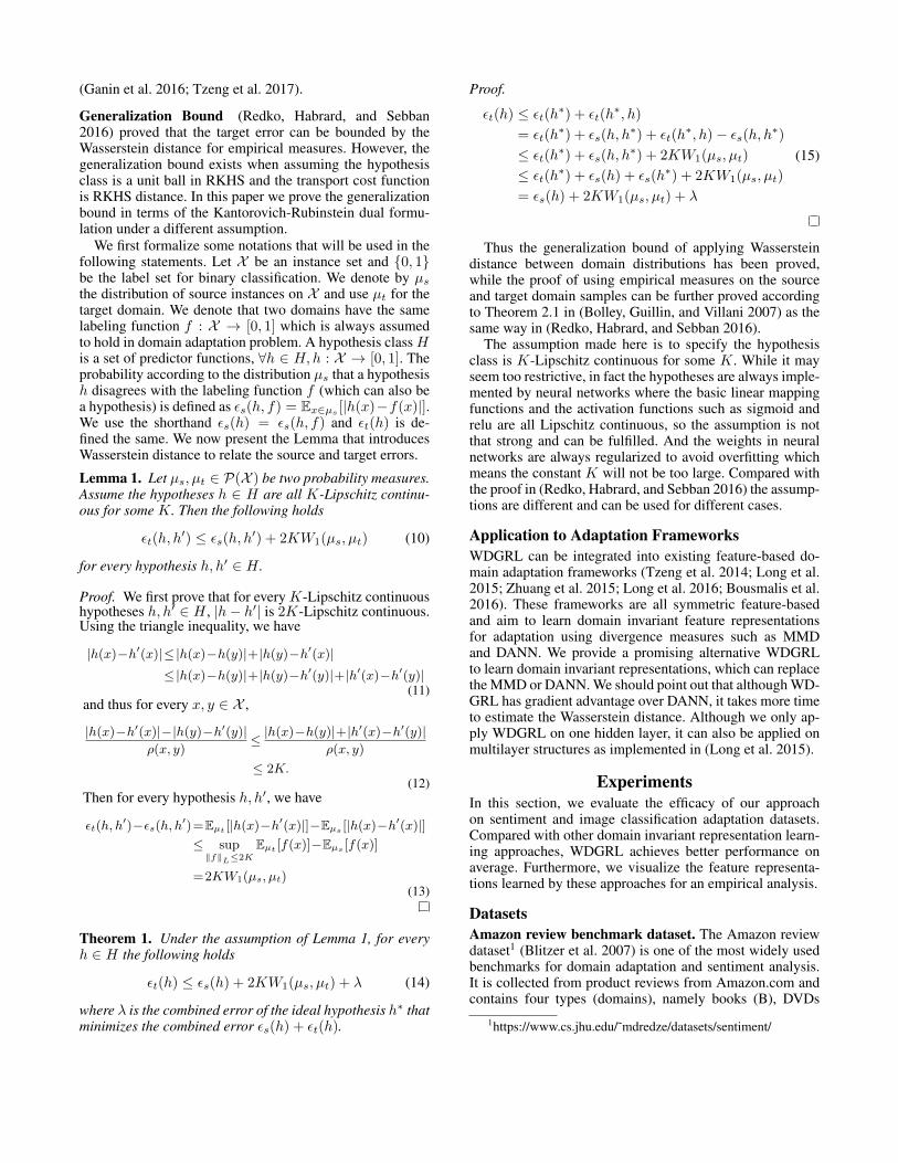
Generalization Bound (Redko, Habrard, and Sebban2016) proved that the target error can be bounded by theWasserstein distance for empirical measures. However, thegeneralization bound exists when assuming the hypothesisclass is a unit ball in RKHS and the transport cost functionis RKHS distance. In this paper we prove the generalizationbound in terms of the Kantorovich-Rubinstein dual formu-lation under a different assumption.

We first formalize some notations that will be used in thefollowing statements. Let X be an instance set and {0, 1}be the label set for binary classification. We denote by µsthe distribution of source instances on X and use µt for thetarget domain. We denote that two domains have the samelabeling function f : X → [0, 1] which is always assumedto hold in domain adaptation problem. A hypothesis classHis a set of predictor functions, ∀h ∈ H,h : X → [0, 1]. Theprobability according to the distribution µs that a hypothesish disagrees with the labeling function f (which can also bea hypothesis) is defined as εs(h, f) = Ex∈µs

[|h(x)−f(x)|].We use the shorthand εs(h) = εs(h, f) and εt(h) is de-fined the same. We now present the Lemma that introducesWasserstein distance to relate the source and target errors.

Lemma 1. Let µs, µt ∈ P(X ) be two probability measures.Assume the hypotheses h ∈ H are all K-Lipschitz continu-ous for some K. Then the following holds

εt(h, h′) ≤ εs(h, h′) + 2KW1(µs, µt) (10)

for every hypothesis h, h′ ∈ H .

Proof. We first prove that for every K-Lipschitz continuoushypotheses h, h′ ∈ H , |h− h′| is 2K-Lipschitz continuous.Using the triangle inequality, we have

|h(x)−h′(x)|≤|h(x)−h(y)|+|h(y)−h′(x)|≤|h(x)−h(y)|+|h(y)−h′(y)|+|h′(x)−h′(y)|

(11)and thus for every x, y ∈ X ,

|h(x)−h′(x)|−|h(y)−h′(y)|ρ(x, y)

≤ |h(x)−h(y)|+|h′(x)−h′(y)|

ρ(x, y)

≤ 2K.(12)

Then for every hypothesis h, h′, we have

εt(h, h′)−εs(h, h′)=Eµt [|h(x)−h

′(x)|]−Eµs [|h(x)−h′(x)|]

≤ sup‖f‖L≤2K

Eµt [f(x)]−Eµs [f(x)]

=2KW1(µs, µt)(13)

Theorem 1. Under the assumption of Lemma 1, for everyh ∈ H the following holds

εt(h) ≤ εs(h) + 2KW1(µs, µt) + λ (14)

where λ is the combined error of the ideal hypothesis h∗ thatminimizes the combined error εs(h) + εt(h).

Proof.

εt(h) ≤ εt(h∗) + εt(h∗, h)

= εt(h∗) + εs(h, h

∗) + εt(h∗, h)− εs(h, h∗)

≤ εt(h∗) + εs(h, h∗) + 2KW1(µs, µt)

≤ εt(h∗) + εs(h) + εs(h∗) + 2KW1(µs, µt)

= εs(h) + 2KW1(µs, µt) + λ

(15)

Thus the generalization bound of applying Wassersteindistance between domain distributions has been proved,while the proof of using empirical measures on the sourceand target domain samples can be further proved accordingto Theorem 2.1 in (Bolley, Guillin, and Villani 2007) as thesame way in (Redko, Habrard, and Sebban 2016).

The assumption made here is to specify the hypothesisclass is K-Lipschitz continuous for some K. While it mayseem too restrictive, in fact the hypotheses are always imple-mented by neural networks where the basic linear mappingfunctions and the activation functions such as sigmoid andrelu are all Lipschitz continuous, so the assumption is notthat strong and can be fulfilled. And the weights in neuralnetworks are always regularized to avoid overfitting whichmeans the constant K will not be too large. Compared withthe proof in (Redko, Habrard, and Sebban 2016) the assump-tions are different and can be used for different cases.

Application to Adaptation FrameworksWDGRL can be integrated into existing feature-based do-main adaptation frameworks (Tzeng et al. 2014; Long et al.2015; Zhuang et al. 2015; Long et al. 2016; Bousmalis et al.2016). These frameworks are all symmetric feature-basedand aim to learn domain invariant feature representationsfor adaptation using divergence measures such as MMDand DANN. We provide a promising alternative WDGRLto learn domain invariant representations, which can replacethe MMD or DANN. We should point out that although WD-GRL has gradient advantage over DANN, it takes more timeto estimate the Wasserstein distance. Although we only ap-ply WDGRL on one hidden layer, it can also be applied onmultilayer structures as implemented in (Long et al. 2015).

ExperimentsIn this section, we evaluate the efficacy of our approachon sentiment and image classification adaptation datasets.Compared with other domain invariant representation learn-ing approaches, WDGRL achieves better performance onaverage. Furthermore, we visualize the feature representa-tions learned by these approaches for an empirical analysis.

DatasetsAmazon review benchmark dataset. The Amazon reviewdataset1 (Blitzer et al. 2007) is one of the most widely usedbenchmarks for domain adaptation and sentiment analysis.It is collected from product reviews from Amazon.com andcontains four types (domains), namely books (B), DVDs

1https://www.cs.jhu.edu/˜mdredze/datasets/sentiment/

(D), electronics (E) and kitchen appliances (K). For eachdomain, there are 2,000 labeled reviews and approximately4,000 unlabeled reviews (varying slightly across domains)and the classes are balanced. In our experiments, for easycomputation, we follow (Chen et al. 2012) to use the 5,000most frequent terms of unigrams and bigrams as the inputand totally A2

4 = 12 adaptation tasks are constructed.Office-Caltech object recognition dataset. The Office-

Caltech dataset2 released by (Gong et al. 2012) is com-prised of 10 common categories shared by the Office-31 andCaltech-256 datasets. In our experiments, we construct 12tasks across 4 domains: Amazon (A), Webcam (W), DSLR(D) and Caltech (C), with 958, 295, 157 and 1,123 im-age samples respectively. In our experiments, Decaf featuresare used as the input. Decaf features (Donahue et al. 2014)are the 4096-dimensional FC7-layer hidden activations ex-tracted by the deep convolutional neural network AlexNet.

Compared ApproachesWe mainly compare our proposed approach with domainadversarial neural network (DANN) (Ganin et al. 2016),maximum mean discrepancy metric (MMD) (Gretton et al.2012) and deep correlation alignment (CORAL) (Sun andSaenko 2016) since these approaches and our proposed WD-GRL all aim at learning the domain invariant feature repre-sentations, which are crucial to reduce the domain discrep-ancy. Other domain adaptation frameworks (Bousmalis et al.2016; Tzeng et al. 2014; Long et al. 2015; Long et al. 2016;Zhuang et al. 2015) are not included in the comparison, be-cause these frameworks focus on adaptation architecture de-sign and all compared approaches can be easily integratedinto these frameworks.

S-only: As an empirical lower bound, we train a modelusing the labeled source data only, and test it on the targettest data directly.

MMD: The MMD metric is a measurement of the di-vergence between two probability distributions from theirsamples by computing the distance of mean embeddings inRKHS.

DANN: DANN is an adversarial representation learningapproach that a domain classifier aims at distinguishing thelearned source/target features while the feature extractortries to confuse the domain classifier. The minimax opti-mization is solved via a gradient reversal layer (GRL).

CORAL: Deep correlation alignment minimizes domaindiscrepancy by aligning the second-order statistics of thesource and target distributions and can be applied to the layeractivations in neural networks.

Implementation DetailsWe implement all our experiments3 using TensorFlow andthe models are all trained with Adam optimizer. We followthe evaluation protocol in (Long et al. 2013) and evaluate allcompared approaches through grid search on the hyperpa-rameter space, and report the best results of each approach.For each approach we use a batch size of 64 samples in total

2https://cs.stanford.edu/˜jhoffman/domainadapt/3Experiment code: https://github.com/RockySJ/WDGRL.

Table 1: Performance (accuracy %) on Amazon reviewdataset.

S-only MMD DANN CORAL WDGRLB→ D 81.09 82.57 82.07 82.74 83.05B→ E 75.23 80.95 78.98 82.93 83.28B→ K 77.78 83.55 82.76 84.81 85.45D→ B 76.46 79.93 79.35 80.81 80.72D→ E 76.24 82.59 81.64 83.49 83.58D→ K 79.68 84.15 83.41 85.35 86.24E→ B 73.37 75.72 75.95 76.91 77.22E→ D 73.79 77.69 77.58 78.08 78.28E→ K 86.64 87.37 86.63 87.87 88.16K→ B 72.12 75.83 75.81 76.95 77.16K→ D 75.79 78.05 78.53 79.11 79.89K→ E 85.92 86.27 86.11 86.83 86.29AVG 77.84 81.22 80.74 82.16 82.43

with 32 samples from each domain, and a fixed learning rate10−4. All compared approaches are combined with a dis-criminator to learn both domain invariant and discriminativerepresentations and to conduct the classification task.

We use standard multi-layer perceptron (MLP) as the ba-sic network architecture. MLP is sufficient to handle all theproblems in our experiments. For Amazon review datasetthe network is designed with one hidden layer of 500 nodes,relu activation function and softmax output function, whilethe network for Office-Caltech dataset has two hidden layersof 500 and 100 nodes. For each dataset the same networkarchitecture is used for all compared approaches and theseapproaches are all applied on the last hidden layer.

For the MMD experiments we follow the suggestions of(Bousmalis et al. 2016) and use a linear combination of 19RBF kernels with the standard deviation parameters rangingfrom 10−6 to 106. As for DANN implementation, we add agradient reversal layer (GRL) and then a domain classifierwith one hidden layer of 100 nodes. And the CORAL ap-proach computes a distance between the second-order statis-tics (covariances) of the source and target features and thedistance is defined as the squared Frobenius norm. For eachapproach, the corresponding loss term is added to the clas-sification loss with a coefficient for the trade-off. And thecoefficients are tuned different to achieve the best results foreach approach.

Our approach is easy to implement according to Algo-rithm 1. In our experiments, the domain critic network is de-signed with a hidden layer of 100 nodes. The training stepsn is 5 which is chosen for fast computation and sufficient op-timization guarantee for the domain critic, and the learningrate for the domain critic is 10−4. We penalize the gradientsnot only at source/target representations but also at the ran-dom points along the straight line between the source andtarget pairs and the coefficient γ is set to 10 as suggested in(Gulrajani et al. 2017).

Results and DiscussionAmazon review benchmark dataset. The challenge ofcross domain sentiment analysis lies in the distribution shiftas different words are used in different domains. Table 1

Table 2: Performance (accuracy %) on Office-Caltechdataset with Decaf features.

S-only MMD DANN CORAL WDGRLA→ C 84.55 88.62 87.80 86.18 86.99A→ D 81.05 90.53 82.46 91.23 93.68A→W 75.59 91.58 77.81 90.53 89.47W→ A 79.82 92.22 82.98 88.39 93.67W→ D 98.25 100 100 100 100W→ C 79.67 88.62 81.30 88.62 89.43D→ A 84.56 90.11 84.70 85.75 91.69D→W 96.84 98.95 98.95 97.89 97.89D→ C 80.49 87.80 82.11 85.37 90.24C→ A 92.35 93.14 93.27 93.01 93.54C→W 84.21 91.58 89.47 92.63 91.58C→ D 87.72 91.23 91.23 89.47 94.74AVG 85.44 92.03 87.67 90.76 92.74

shows the detailed comparison results of these approachesin 12 transfer tasks. As we can see, our proposed WDGRLoutperforms all other compared approaches in 10 out of 12domain adaptation tasks, and it achieves the second high-est scores in the remaining 2 tasks. We find that as adver-sarial adaptation approaches, WDGRL outperforms DANN,which is consistent with our theoretical analysis that WD-GRL has more reliable gradients. MMD and CORAL areboth non-parametric and have lower computational cost thanWDGRL, while their classification performances are alsolower than WDGRL.

Office-Caltech object recognition dataset. Table 2shows the results of our experiments on Office-Caltechdataset. We observe that our approach achieves better per-formance than other compared approaches on most tasks.Office-Caltech dataset is small since there are only hundredsof images in one domain and it is a 10-class classificationproblem. Thus we can draw a conclusion that the empiri-cal Wasserstein distance can also be applied to small-scaledatasets adaptation effectively. We note that CORAL per-forms better than MMD in Amazon review dataset while itperforms worse than MMD in Office-Caltech dataset. A pos-sible reason is that the reasonable covariance alignment ap-proach requires large samples. On the other hand, we can seethat these different approaches have different performanceson different adaptation tasks.

Feature VisualizationWe randomly choose the D→E domain adaptation task ofAmazon review dataset and plot in Figure 2 the t-SNE visu-alization following (Donahue et al. 2014; Long et al. 2016)to visualize the learned feature representations. In these fig-ures, red and blue points represent positive and negativesamples of the source domain, purple and green points rep-resent positive and negative samples of the target domain. Atransferable feature mapping should cluster red (blue) andpurple (green) points together, and meanwhile classificationcan be easily conducted between purple and green points.We can see that almost all approaches learn discriminativeand domain invariant feature representations to some extent.And representations learned by WDGRL are more transfer-

0.0 0.2 0.4 0.6 0.8 1.0

0.0

0.2

0.4

0.6

0.8

1.0

(a) t-SNE of DANN features0.0 0.2 0.4 0.6 0.8 1.0

0.0

0.2

0.4

0.6

0.8

1.0

(b) t-SNE of MMD features

0.0 0.2 0.4 0.6 0.8 1.0

0.0

0.2

0.4

0.6

0.8

1.0

(c) t-SNE of CORAL features0.0 0.2 0.4 0.6 0.8 1.0

0.0

0.2

0.4

0.6

0.8

1.0

(d) t-SNE of WDGRL features

Figure 2: Feature visualization of the D→E task in Amazonreview dataset.

able since the classes between the source and target domainsalign better and the region where purple and green pointsmix together is smaller.

Conclusions

In this paper, we propose a new adversarial approach WD-GRL to learn domain invariant feature representations fordomain adaptation. WDGRL can effectively reduce the do-main discrepancy taking advantage of the gradient propertyof Wasserstein distance and the transferability is guaran-teed by the generalization bound. Our proposed approachcould be further integrated into other domain adaptationframeworks (Bousmalis et al. 2016; Tzeng et al. 2014;Long et al. 2015; Long et al. 2016; Zhuang et al. 2015) toattain better transferability. Empirical results on sentimentand image classification domain adaptation datasets demon-strate that WDGRL outperforms the state-of-the-art domaininvariant feature learning approaches. From feature visual-ization, one can easily observe that WDGRL yields domaininvariant yet target-discriminative feature representations. Infuture work, we will investigate more sophisticated architec-tures for tasks on image data as well as integrate WDGRLinto existing adaptation frameworks.

Acknowledgement

This work is financially supported by NSFC (61702327) andShanghai Sailing Program (17YF1428200).

References[Ajakan et al. 2014] Ajakan, H.; Germain, P.; Larochelle, H.;Laviolette, F.; and Marchand, M. 2014. Domain-adversarialneural networks. arXiv:1412.4446.

[Arjovsky, Chintala, and Bottou 2017] Arjovsky, M.; Chin-tala, S.; and Bottou, L. 2017. Wasserstein gan.arXiv:1701.07875.

[Ben-David et al. 2007] Ben-David, S.; Blitzer, J.; Crammer,K.; and Pereira, F. 2007. Analysis of representations fordomain adaptation. In NIPS.

[Ben-David et al. 2010] Ben-David, S.; Blitzer, J.; Crammer,K.; Kulesza, A.; Pereira, F.; and Vaughan, J. W. 2010. Atheory of learning from different domains. Machine learn-ing.

[Blitzer et al. 2007] Blitzer, J.; Dredze, M.; Pereira, F.; et al.2007. Biographies, bollywood, boom-boxes and blenders:Domain adaptation for sentiment classification. In ACL.

[Bolley, Guillin, and Villani 2007] Bolley, F.; Guillin, A.;and Villani, C. 2007. Quantitative concentration inequalitiesfor empirical measures on non-compact spaces. ProbabilityTheory and Related Fields.

[Bousmalis et al. 2016] Bousmalis, K.; Trigeorgis, G.; Sil-berman, N.; Krishnan, D.; and Erhan, D. 2016. Domainseparation networks. In NIPS.

[Chen et al. 2012] Chen, M.; Xu, Z.; Weinberger, K.; andSha, F. 2012. Marginalized denoising autoencoders for do-main adaptation. arXiv:1206.4683.

[Chen, Chen, and Weinberger 2011] Chen, M.; Chen, Y.; andWeinberger, K. Q. 2011. Automatic feature decompositionfor single view co-training. In ICML.

[Chen, Weinberger, and Blitzer 2011] Chen, M.; Wein-berger, K. Q.; and Blitzer, J. 2011. Co-training for domainadaptation. In NIPS.

[Chu, De la Torre, and Cohn 2013] Chu, W.-S.; De la Torre,F.; and Cohn, J. F. 2013. Selective transfer machine forpersonalized facial action unit detection. In CVPR.

[Courty et al. 2017] Courty, N.; Flamary, R.; Tuia, D.; andRakotomamonjy, A. 2017. Optimal transport for domainadaptation. IEEE transactions on pattern analysis and ma-chine intelligence.

[Courty, Flamary, and Tuia 2014] Courty, N.; Flamary, R.;and Tuia, D. 2014. Domain adaptation with regularizedoptimal transport. In ECML/PKDD.

[Donahue et al. 2014] Donahue, J.; Jia, Y.; Vinyals, O.; Hoff-man, J.; Zhang, N.; Tzeng, E.; and Darrell, T. 2014. Decaf:A deep convolutional activation feature for generic visualrecognition. In ICML.

[Duan, Xu, and Chang 2012] Duan, L.; Xu, D.; and Chang,S.-F. 2012. Exploiting web images for event recognitionin consumer videos: A multiple source domain adaptationapproach. In CVPR. IEEE.

[Ganin et al. 2016] Ganin, Y.; Ustinova, E.; Ajakan, H.; Ger-main, P.; Larochelle, H.; Laviolette, F.; Marchand, M.; andLempitsky, V. 2016. Domain-adversarial training of neuralnetworks. JMLR.

[Glorot, Bordes, and Bengio 2011] Glorot, X.; Bordes, A.;and Bengio, Y. 2011. Domain adaptation for large-scale sen-timent classification: A deep learning approach. In ICML.

[Gong et al. 2012] Gong, B.; Shi, Y.; Sha, F.; and Grauman,K. 2012. Geodesic flow kernel for unsupervised domainadaptation. In CVPR. IEEE.

[Goodfellow et al. 2014] Goodfellow, I.; Pouget-Abadie, J.;Mirza, M.; Xu, B.; Warde-Farley, D.; Ozair, S.; Courville,A.; and Bengio, Y. 2014. Generative adversarial nets. InNIPS.

[Gretton et al. 2012] Gretton, A.; Borgwardt, K. M.; Rasch,M. J.; Scholkopf, B.; and Smola, A. 2012. A kernel two-sample test. JMLR.

[Gulrajani et al. 2017] Gulrajani, I.; Ahmed, F.; Arjovsky,M.; Dumoulin, V.; and Courville, A. 2017. Improved train-ing of wasserstein gans. arXiv:1704.00028.

[Hoffman et al. 2014] Hoffman, J.; Rodner, E.; Donahue, J.;Kulis, B.; and Saenko, K. 2014. Asymmetric and cate-gory invariant feature transformations for domain adapta-tion. IJCV.

[Huang et al. 2007] Huang, J.; Smola, A. J.; Gretton, A.;Borgwardt, K. M.; Scholkopf, B.; et al. 2007. Correctingsample selection bias by unlabeled data. NIPS.

[Kandemir 2015] Kandemir, M. 2015. Asymmetric transferlearning with deep gaussian processes. In ICML.

[Long et al. 2013] Long, M.; Wang, J.; Ding, G.; Sun, J.; andYu, P. S. 2013. Transfer feature learning with joint distri-bution adaptation. In The IEEE International Conference onComputer Vision (ICCV).

[Long et al. 2015] Long, M.; Cao, Y.; Wang, J.; and Jordan,M. 2015. Learning transferable features with deep adapta-tion networks. In ICML.

[Long et al. 2016] Long, M.; Wang, J.; Cao, Y.; Sun, J.; andPhilip, S. Y. 2016. Deep learning of transferable represen-tation for scalable domain adaptation. TKDE.

[Luo et al. 2017] Luo, L.; Wang, X.; Hu, S.; Wang, C.; Tang,Y.; and Chen, L. 2017. Close yet distinctive domain adapta-tion. arXiv:1704.04235.

[Mansour, Mohri, and Rostamizadeh 2009] Mansour, Y.;Mohri, M.; and Rostamizadeh, A. 2009. Domain adaptationwith multiple sources. In NIPS.

[Narayanan and Mitter 2010] Narayanan, H., and Mitter, S.2010. Sample complexity of testing the manifold hypothe-sis. In NIPS.

[Pan and Yang 2010] Pan, S. J., and Yang, Q. 2010. A surveyon transfer learning. IEEE Transactions on knowledge anddata engineering.

[Redko, Habrard, and Sebban 2016] Redko, I.; Habrard, A.;and Sebban, M. 2016. Theoretical analysis of domain adap-tation with optimal transport. arXiv:1610.04420.

[Rozantsev, Salzmann, and Fua 2016] Rozantsev, A.; Salz-mann, M.; and Fua, P. 2016. Beyond sharing weights fordeep domain adaptation. arXiv:1603.06432.

[Sun and Saenko 2016] Sun, B., and Saenko, K. 2016. Deep

coral: Correlation alignment for deep domain adaptation. InECCV 2016 Workshops. Springer.

[Sun, Feng, and Saenko 2016] Sun, B.; Feng, J.; and Saenko,K. 2016. Return of frustratingly easy domain adaptation. InAAAI.

[Tzeng et al. 2014] Tzeng, E.; Hoffman, J.; Zhang, N.;Saenko, K.; and Darrell, T. 2014. Deep domain confusion:Maximizing for domain invariance. arXiv:1412.3474.

[Tzeng et al. 2017] Tzeng, E.; Hoffman, J.; Saenko, K.; andDarrell, T. 2017. Adversarial discriminative domain adapta-tion. arXiv:1702.05464.

[Villani 2008] Villani, C. 2008. Optimal transport: old andnew.

[Weiss, Khoshgoftaar, and Wang 2016] Weiss, K.; Khosh-goftaar, T. M.; and Wang, D. 2016. A survey of transferlearning. Journal of Big Data.

[Zhuang et al. 2015] Zhuang, F.; Cheng, X.; Luo, P.; Pan,S. J.; and He, Q. 2015. Supervised representation learning:Transfer learning with deep autoencoders. In IJCAI.

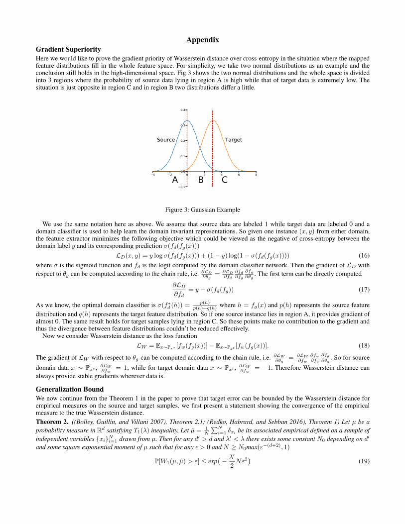
AppendixGradient SuperiorityHere we would like to prove the gradient priority of Wasserstein distance over cross-entropy in the situation where the mappedfeature distributions fill in the whole feature space. For simplicity, we take two normal distributions as an example and theconclusion still holds in the high-dimensional space. Fig 3 shows the two normal distributions and the whole space is dividedinto 3 regions where the probability of source data lying in region A is high while that of target data is extremely low. Thesituation is just opposite in region C and in region B two distributions differ a little.

4 2 0 2 4 6 8

0.1

0.0

0.1

0.2

0.3

0.4

CA B

TargetSource

Figure 3: Gaussian Example

We use the same notation here as above. We assume that source data are labeled 1 while target data are labeled 0 and adomain classifier is used to help learn the domain invariant representations. So given one instance (x, y) from either domain,the feature extractor minimizes the following objective which could be viewed as the negative of cross-entropy between thedomain label y and its corresponding prediction σ(fd(fg(x)))

LD(x, y) = y log σ(fd(fg(x))) + (1− y) log(1− σ(fd(fg(x)))) (16)where σ is the sigmoid function and fd is the logit computed by the domain classifier network. Then the gradient of LD withrespect to θg can be computed according to the chain rule, i.e. ∂LD

∂θg= ∂LD

∂fd

∂fd∂fg

∂fg∂θg

. The first term can be directly computed

∂LD∂fd

= y − σ(fd(fg)) (17)

As we know, the optimal domain classifier is σ(f∗d (h)) = p(h)p(h)+q(h) where h = fg(x) and p(h) represents the source feature

distribution and q(h) represents the target feature distribution. So if one source instance lies in region A, it provides gradient ofalmost 0. The same result holds for target samples lying in region C. So these points make no contribution to the gradient andthus the divergence between feature distributions couldn’t be reduced effectively.

Now we consider Wasserstein distance as the loss functionLW = Ex∼Pxs [fw(fg(x))]− Ex∼Pxt [fw(fg(x))]. (18)

The gradient of LW with respect to θg can be computed according to the chain rule, i.e. ∂LW

∂θg= ∂LW

∂fw

∂fw∂fg

∂fg∂θg

. So for source

domain data x ∼ Pxs , ∂LW

∂fw= 1; while for target domain data x ∼ Pxt , ∂LW

∂fw= −1. Therefore Wasserstein distance can

always provide stable gradients wherever data is.

Generalization BoundWe now continue from the Theorem 1 in the paper to prove that target error can be bounded by the Wasserstein distance forempirical measures on the source and target samples. we first present a statement showing the convergence of the empiricalmeasure to the true Wasserstein distance.Theorem 2. ((Bolley, Guillin, and Villani 2007), Theorem 2.1; (Redko, Habrard, and Sebban 2016), Theorem 1) Let µ be aprobability measure in Rd satisfying T1(λ) inequality. Let µ = 1

N

∑Ni=1 δxi

be its associated empirical defined on a sample ofindependent variables {xi}Ni=1 drawn from µ. Then for any d′ > d and λ′ < λ there exists some constant N0 depending on d′

and some square exponential moment of µ such that for any ε > 0 and N ≥ N0max(ε−(d+2), 1)

P[W1(µ, µ) > ε] ≤ exp(− λ′

2Nε2

)(19)

where d′, λ′ can be calculated explicitly.

Now we can follow the Theorem 1 and Theorem 2 to prove that target error can be bounded by the Wasserstein distance forempirical measures on the source and target samples as the process of the proof of the Theorem 3. in (Redko, Habrard, andSebban 2016).

Theorem 3. Under the assumption of Lemma 1, let two probability measures satisfy T1(λ) inequality, Xs and Xt be twosamples of size Ns and Nt drawn i.i.d from µs and µt resepectively. Let µs = 1

Ns

∑Ns

i=1 δxsi

and µt = 1Nt

∑Nt

i=1 δxti

be theassociated empirical measures. Then for any d′ > d and λ′ < λ there exists some constant N0 depending on d′ such that forany δ > 0 and min(Ns,Nt) ≥ N0max(δ−(d′+2), 1) with probability at least 1− δ for all h the followingt holds:

εt(h) ≤ εs(h) + 2KW1(µs, µt) + λ+ 2K

√2log

(1

δ

)/λ′(√

1

Ns+

√1

Nt

)(20)

where λ is the combined error of the ideal hypothesis h∗ that minimizes the combined error of εs(h) + εt(h).

Proof.εt(h) ≤ εs(h) + 2KW1(µs, µt) + λ

≤ εs(h) + 2KW1(µs, µs) + 2KW1(µs, µt) + λ

≤ εs(h) + 2K

√2log

(1

δ

)/Nsλ′ + 2KW1(µs, µt) + 2KW1( ˆµt, µt) + λ

≤ εs(h) + 2KW1(µs, µt) + λ+ 2K

√2log

(1

δ

)/λ′(√

1

Ns+

√1

Nt

)(21)

More Experiment ResultsSynthetic data. We generate a synthetic dataset to show the superior gradient advantage of WDGRL over DANN. In the paper,we claim that when two representation distributions are distant or have regions they differ a lot, DANN will have gradientvanishing problem while WDGRL still provides the stable gradient. It is a little difficult to fully realize such situations, sowe design a rather restrictive experiment. However, this toy experiment does verify DANN may fail in some situations whileWDGRL can work. We visualize the data input in Figure 4(a) with 2000 samples for each domain. And from Figure 4(b) wefind that if we adopt DANN the domain classifier can distinguish two domain data well and the DANN loss decreases to nearly0 as the training process continues. In such situation, the domain classifier can provide poor gradient. As shown in 4(c), ourWDGRL approach can effectively classify the target data while DANN fails.

(a) input visualization (b) DANN loss and accuracy (c) Performance on target domain

Figure 4: Synthetic experiment.

Office-Caltech dataset with SURF features. Table 3 shows the result of our experiments on Office-Caltech dataset withSURF features.

Email spam filtering dataset. The email spam filtering dataset 4 released by ECML/PKDD 2006 discovery challenge con-tains 4 separate user inboxes. From public inbox (source domain) 4,000 labeled training samples were collected, among which

4http://www.ecmlpkdd2006.org/challenge.html

Table 3: Performance (accuracy %) on Office-Caltech dataset with Decaf featuresS-only MMD DANN D-CORAL WDGRL

A→ C 43.19 44.08 44.97 44.97 45.86A→ D 35.03 41.40 41.40 40.13 44.59A→W 35.23 37.29 38.64 38.31 40.68W→ A 30.06 34.13 34.13 34.86 32.15W→ D 80.25 84.71 82.80 84.08 81.53W→ C 30.19 30.72 32.68 33.30 31.08C→W 36.95 40.34 43.39 40.00 42.37C→ A 52.92 54.80 54.91 53.44 55.22C→ D 45.86 47.13 47.77 47.13 48.41D→W 69.50 73.56 74.24 73.90 76.95D→ A 31.21 32.46 31.63 31.52 35.60D→ C 30.37 30.72 32.24 31.52 32.59AVG 43.4 45.95 46.57 46.10 47.25

half samples are spam emails and the other half non-spam ones. The test samples were collected from 3 private inboxes (targetdomains), each of which consists of 2,500 samples. In our experiments, 3 cross-domain tasks are constructed from the publicinbox to the private inboxes. We choose the 5,067 most frequent terms as features and 4 test samples were deleted as a result ofnot containing any of these terms. Experimenting on the 3 tasks by transferring from public to private groups of private inboxesu1 ∼ u3, we found our method does achieve better performance than MMD, DANN and D-CORAL, which is demonstrated inTable 4. We can see from this result that all these approaches can reach the goal of learning the transferable features for they alloutperform the source only baseline at least 9%. Among them, MMD and DANN achieve almost the same performance whileWDGRL further boosts the performance by a rate of 2.90%.

Table 4: Performance (Accuracy %) on email spam datasetS only MMD DANN D-CORAL WDGRL

P→ u1 69.63 80.95 83.27 79.71 85.67P→ u2 76.01 85.98 85.74 83.83 88.26P→ u3 81.24 94.08 91.92 89.80 95.76

AVG 75.63 87.00 86.98 84.45 89.90

Newsgroup classification dataset. The 20 newsgroups dataset 5 is a collection of 18,774 newsgroup documents across 6top categories and 20 subcategories in a hierarchical structure. In our experiments, we adopt a similar setting as (?). The taskis to classify top categories and the four largest top categories (comp, rec, sci, talk) are chosen for evaluation. Specifically, foreach top category, the largest subcategory is selected as the source domain while the second largest subcategory is chosen asthe target domain. Moreover, the largest category comp is considered as the positive class and one of the three other categoriesas the negative class.

The distribution shift across newsgroups is caused by category specific words. Notice the construction of our domain adap-tation tasks which aim to classify the top categories while the adaptation exists between the subcategories. It makes sense thatthere exist more differences among top categories than those among subcategories which implies that classification is not thatsensitive to the subcategories and thus enables the ease of domain adaptation. Table 5 gives the information of performance onthe 20newsgroup dataset from which we can find that the comparison methods are almost neck and neck, which is consistentwith our previous observation.

Table 5: Performance (Accuracy %) on 20 newsgroup datasetS only MMD DANN D-CORAL WDGRL

C vs. R 81.62 97.85 98.10 97.57 98.35C vs. S 74.01 87.52 90.57 84.20 91.33C vs. T 94.44 96.96 97.75 97.22 97.62AVG 83.36 94.11 95.47 93.00 95.77

5http://qwone.com/˜jason/20Newsgroups/