Water Quality Method · PDF fileThis Method Statement presents information on the approach for...

Annex 6A

Water Quality Method Statement

LNG RECEIVING TERMINAL AND ASSOCIATED FACILITIES PART 3 – BLACK POINT EIA

SECTION 6 ANNEX 6A – WATER QUALITY METHOD STATEMENT

CONTENTS

1 INTRODUCTION 1

1.1 INTERPRETATION OF THE REQUIREMENTS: KEY ISSUES AND CONSTRAINTS 1 1.2 MODEL SELECTION 1 1.3 COASTLINE & BATHYMETRY 4 1.4 VECTOR INFORMATION 6 1.5 INFORMATION ON MODEL INPUTS 7 1.6 UNCERTAINTIES IN ASSESSMENT METHODOLOGIES 7

2 WATER SENSITIVE RECEIVERS 8

3 CONSTRUCTION PHASE 9

3.1 WORKING TIME 10 3.2 OVERVIEW OF DREDGING PLANTS 10 3.3 CONSTRUCTION SCENARIOS 13 3.4 SEWAGE DISCHARGE 17

4 OPERATIONAL PHASE 18

4.1 THERMAL AND ANTIFOULANT DISCHARGE 19 4.2 SEWAGE DISCHARGE 20 4.3 MAINTENANCE DREDGING 21 4.4 ACCIDENTAL FUEL SPILLAGE 22

5 CUMULATIVE IMPACTS 24

6 INPUT PARAMETERS 25

6.1 SEDIMENT PARAMETERS 25

7 SCENARIOS 26

7.1 CONSTRUCTION PHASE 26

APPENDIX

Appendix 6A Information on the Model Inputs

Appendix 6B Information on the CORMIX Model Simulation



0018180_EIA PART 3 S6 ANNEX 6A_V6.DOC 11 DEC 2006

1

1 INTRODUCTION

This Method Statement presents information on the approach for the water

quality assessment and modelling works for the study. The methodology

has been based on the following three focus areas, as follows:

• Model Selection;

• Input Data; and,

• Scenarios.

1.1 INTERPRETATION OF THE REQUIREMENTS: KEY ISSUES AND CONSTRAINTS

The objectives of the modelling exercise are to assess:

• Effects of construction, which comprises the study of the dispersion of

sediments released during construction;

• Effects of operation due to reclamations (affecting flows and potentially

water quality due to changing flows); discharges (potentially affecting

temperatures and water quality due to chlorine or other antifoulants); and

maintenance dredging (potentially increasing suspended solids in water

column);

• Any residual impacts, which include any change in hydrodynamic

regime; and

• Any cumulative impacts due to other projects or activities within the

study area.

The construction and operational effects have been studied by means of

mathematical modelling using existing models that have been set up by WL |

Delft Hydraulics (Delft) on behalf of the Environmental Protection

Department (EPD) or approved by the EPD for use in environmental

assessments.

1.2 MODEL SELECTION

The existing Western Harbour Model of the Delft 3D water quality (WAQ)

and hydrodynamic suite of models have been used to simulate effects on

hydrodynamics and water quality. These models have been calibrated as

part of the Landfill Extension Study.

The WAQ model has been used to simulate water quality impacts during

construction and operation of the facility. The existing Update model has the

required spatial extent. The existing grid of the model in the vicinity of Black

Point is shown in Figure A1.1.




2

Figure A1.1 Model Grid of the Update Model in the Vicinity of Black Point

As seen in Figure A1.1, the grid size of the existing model near the site is in the

order of about 300m. The extent of the reclamation at the site is such that it

covers approximately one grid cell. It was therefore considered appropriate

to carry out refinement of the water quality and hydrodynamic grids to

provide improved resolution (less than 75m) in some of the key areas of

interest. The refinements of the model grid of the Update Model in the

vicinity of Black Point are shown in Figure A1.2.

4 km




3

Figure A1.2 Model Grid of the Update Model in the Vicinity of Black Point




4

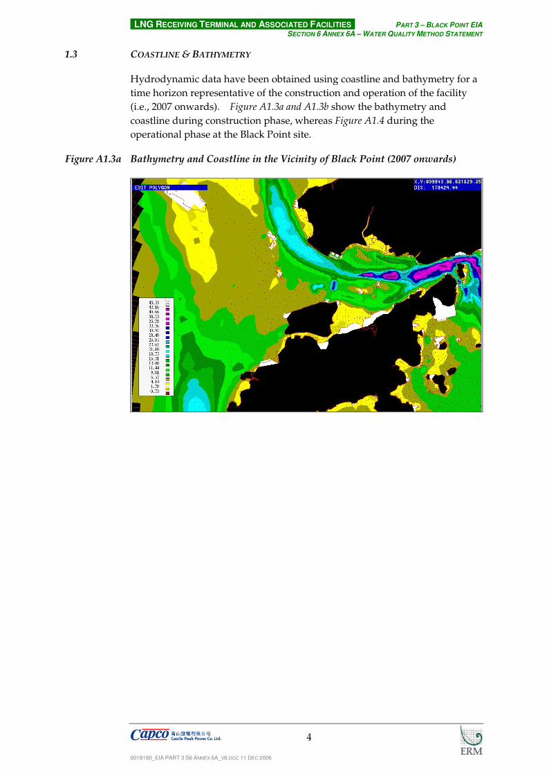
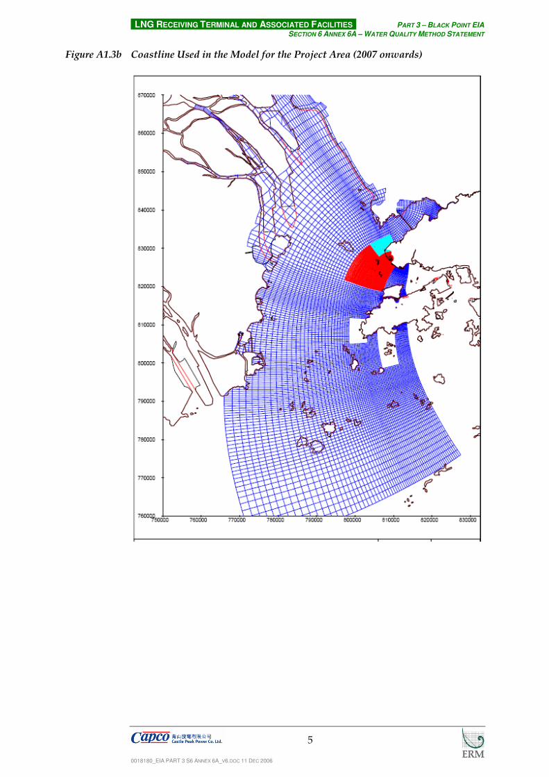
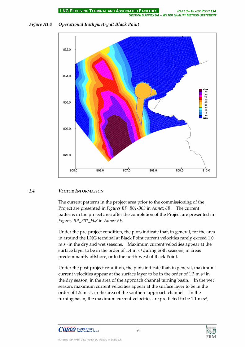
1.3 COASTLINE & BATHYMETRY

Hydrodynamic data have been obtained using coastline and bathymetry for a

time horizon representative of the construction and operation of the facility

(i.e., 2007 onwards). Figure A1.3a and A1.3b show the bathymetry and

coastline during construction phase, whereas Figure A1.4 during the

operational phase at the Black Point site.

Figure A1.3a Bathymetry and Coastline in the Vicinity of Black Point (2007 onwards)




5

Figure A1.3b Coastline Used in the Model for the Project Area (2007 onwards)




6

Figure A1.4 Operational Bathymetry at Black Point

1.4 VECTOR INFORMATION

The current patterns in the project area prior to the commissioning of the

Project are presented in Figures BP_B01-B08 in Annex 6B. The current

patterns in the project area after the completion of the Project are presented in

Figures BP_F01_F08 in Annex 6F.

Under the pre-project condition, the plots indicate that, in general, for the area

in around the LNG terminal at Black Point current velocities rarely exceed 1.0

m s-1 in the dry and wet seasons. Maximum current velocities appear at the

surface layer to be in the order of 1.4 m s-1 during both seasons, in areas

predominantly offshore, or to the north-west of Black Point.

Under the post-project condition, the plots indicate that, in general, maximum

current velocities appear at the surface layer to be in the order of 1.3 m s-1 in

the dry season, in the area of the approach channel turning basin. In the wet

season, maximum current velocities appear at the surface layer to be in the

order of 1.5 m s-1, in the area of the southern approach channel. In the

turning basin, the maximum current velocities are predicted to be 1.1 m s-1.




7

1.5 INFORMATION ON MODEL INPUTS

Details on the model input parameters are presented in Appendix 6A in Annex

6A.

1.6 UNCERTAINTIES IN ASSESSMENT METHODOLOGIES

Uncertainties in the assessment of the impacts from suspended sediment

plumes should be considered when drawing conclusions from the assessment.

In carrying out the assessment, the worst case assumptions have been made in

order to provide a conservative assessment of environmental impacts. These

assumptions are as follows:

• The assessment is based on the peak dredging and filling rates. In

reality, these will only occur for short period of time; and,

• The calculations of loss rates of sediment to suspension are based on

conservative estimates for the types of plant and methods of working.

The conservative assumptions presented above allow a prudent approach to

be applied to the water quality assessment.

The following uncertainties has not included in the modelling assessment.

• Ad hoc navigation of marine traffic;

• Near shore scouring of bottom sediment; and

• Access of marine barges back and forth the site.




8

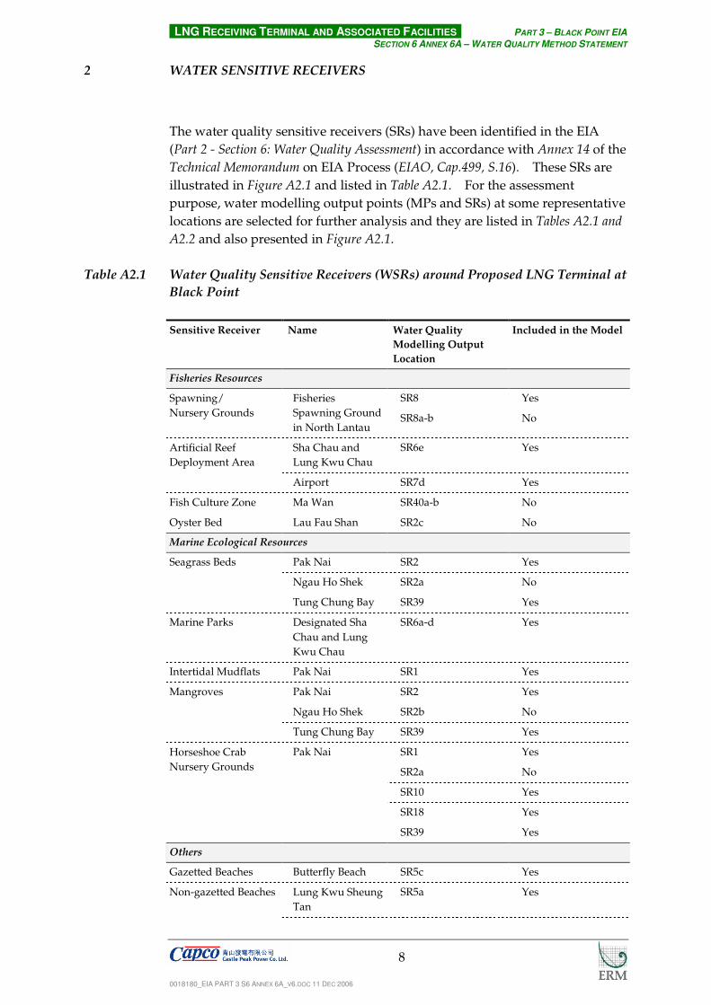
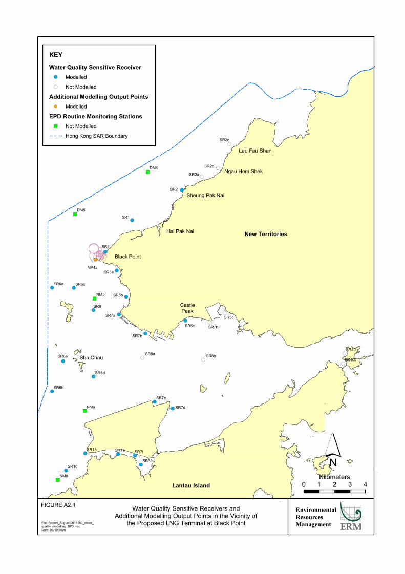
2 WATER SENSITIVE RECEIVERS

The water quality sensitive receivers (SRs) have been identified in the EIA

(Part 2 - Section 6: Water Quality Assessment) in accordance with Annex 14 of the

Technical Memorandum on EIA Process (EIAO, Cap.499, S.16). These SRs are

illustrated in Figure A2.1 and listed in Table A2.1. For the assessment

purpose, water modelling output points (MPs and SRs) at some representative

locations are selected for further analysis and they are listed in Tables A2.1 and

A2.2 and also presented in Figure A2.1.

Table A2.1 Water Quality Sensitive Receivers (WSRs) around Proposed LNG Terminal at

Black Point

Sensitive Receiver Name Water Quality

Modelling Output

Location

Included in the Model

Fisheries Resources

SR8 Yes Spawning/

Nursery Grounds

Fisheries

Spawning Ground

in North Lantau SR8a-b No

Artificial Reef

Deployment Area

Sha Chau and

Lung Kwu Chau

SR6e Yes

Airport SR7d Yes

Fish Culture Zone Ma Wan SR40a-b No

Oyster Bed Lau Fau Shan SR2c No

Marine Ecological Resources

Seagrass Beds Pak Nai SR2 Yes

Ngau Ho Shek SR2a No

Tung Chung Bay SR39 Yes

Marine Parks Designated Sha

Chau and Lung

Kwu Chau

SR6a-d Yes

Intertidal Mudflats Pak Nai SR1 Yes

Mangroves Pak Nai SR2 Yes

Ngau Ho Shek SR2b No

Tung Chung Bay SR39 Yes

Pak Nai SR1 Yes Horseshoe Crab

Nursery Grounds SR2a No

SR10 Yes

SR18 Yes

SR39 Yes

Others

Gazetted Beaches Butterfly Beach SR5c Yes

Non-gazetted Beaches Lung Kwu Sheung

Tan

SR5a Yes

�)

�)

�)

�)

�)

!(

!(

!(

!(

!(

!(

!(

!(

!( !(

!(

!(

!(

!(

!(

!(

!( !(

!(

!(

!(

(

(

(

!(

((

(

(

(

(

!(

Lantau Island

New Territories

Black Point

Hai Pak Nai

Sheung Pak Nai

CastlePeak

Sha Chau

Ngau Hom Shek

Lau Fau Shan

SR8

SR4

SR2

SR1

SR2c

SR2b

SR2a

MP4a

SR5d

SR6d

SR5b

SR5a

SR6cSR6a

SR12

SR10

SR18

SR6e

SR6b

SR39

SR7fSR7e

SR7d

SR7c

SR5c

SR7b

SR7a

SR7h

SR8a SR8b

SR40b

SR40a

NM8

NM6

NM5

DM5

DM4

Environmental

Resources

Management

Water Quality Sensitive Receivers andAdditional Modelling Output Points in the Vicinity of

the Proposed LNG Terminal at Black Point

FIGURE A2.1

File: Report_August/0018180_water_quality_modelling_BP3.mxdDate: 05/10/2006

KEY

Water Quality Sensitive Receiver

!( Modelled

( Not Modelled

Additional Modelling Output Points

!( Modelled

EPD Routine Monitoring Stations

�) Not Modelled

Hong Kong SAR Boundary

0 1 2 3 4Kilometers

�




9


Modelling Output

Location


Lung Kwu Tan SR5b Yes

Seawater Intakes Black Point Power

Station

SR4 Yes

Castle Peak Power

Station

SR7a Yes

Tuen Mun Area 38 SR7b Yes

Airport SR7c-f Yes

Tuen Mun WSD SR7h No

Table A2.2 Water Quality Modelling Output Points (MPs) around Proposed LNG

Terminal at Black Point


Modelling Output

Location


Seawater Intakes Operational Phase

LNG Intake

MP4a Yes

Table A2.3 EPD Routine Water Quality Monitoring Stations in the Vicinity of the

Project Area

EPD Monitoring Stations Respective WCZ Included in the Model

Seawater Intakes Operational Phase LNG

Intake

Yes

3 CONSTRUCTION PHASE

For the construction phase the WAQ model has been used to directly simulate

the following parameters:

• suspended sediments; and

• sediment deposition.

It is assumed that the worst-case construction phase impacts will be at the

commencement of dredging, when there is no depression formed to trap

sediments disturbed during dredging.

Note that DO, TIN and NH3-N are calculated based on the modelled

maximum SS concentrations as shown in Section 6: Water Quality Impact

Assessment.




10

3.1 WORKING TIME

The estimation of programme for dredging activity at Black Point is based on

the assumption of a 16 working hours per day with 6 working days per week.

An arrangement of 24 working hours and 7 working days is unlikely to be

feasible for Black Point due to the potential noise impact generated by barges

travelling at night to the villages located in close proximity to the route of

Black Point and the dumping sites at South Cheung Chau.

3.2 OVERVIEW OF DREDGING PLANTS

3.2.1 Grab Dredgers

Grab dredgers will be utilised in the dredging works for the reclamation

works at the terminal as well as the navigation channel, turning circle and

berthing box. Also the submarine water mains and some of the sections of

the submarine pipeline may need to be pre-trenched and this is likely to be

done utilising a grab dredger.

Grab dredgers may release sediment into suspension by the following

mechanisms:

• Impact of the grab on the seabed as it is lowered;

• Washing of sediment off the outside of the grab as it is raised through the

water column and when it is lowered again after being emptied;

• Leakage of water from the grab as it is hauled above the water surface;

• Spillage of sediment from over-full grabs;

• Loss from grabs which cannot be fully closed due to the presence of

debris;

• Release by splashing when loading barges by careless, inaccurate

methods; and

• Disturbance of the seabed as the closed grab is removed.

In the transport of dredging materials, sediment may be lost through leakage

from barges. However, dredging permits in Hong Kong include

requirements that barges used for the transport of dredging materials have

bottom-doors that are properly maintained and have tight-fitting seals in

order to prevent leakage. Given this requirement, sediment release during

transport is not proposed for modelling and its impact on water quality is not

addressed under this Study.

Sediment is also lost to the water column when discharging material at

disposal sites. The amount that is lost depends on a large number of factors

including material characteristics, the speed and manner in which it is




11

discharged from the vessel, and the characteristics of the disposal sites. As

impacts due to disposal operations at potential disposal sites have been

assessed under separate studies, they are not addressed further in this

document.

The modelling of dredging using grabs has assumed a loss rate of 17 kg m-3

dredged sediment. This rate is representative of grab dredgers (with a closed

grab size of approximately 8 m3 minimum) working in areas without debris.

It is possible that the contractor may utilise a larger grab in the construction.

The loss rate for a larger grab is lower than for a smaller grab.

Generally, a split-bottom barge could have a capacity of 900 m³. A bulk

factor of 1.3 would normally be applied, giving a dredging rate of 700 m³ per

barge. The hopper dry density for an 800 to 1,000 m3 capacity barge is

around 0.75 to 1.24 ton m-3. Assuming 16 working hours per day for Black

Point, with allowance on the demobilisation of filled barge and remobilisation

of empty barges, a maximum of 7 barges could be filled per day. Therefore,

the average daily dredging rate would be approximately 4,900 m3. The use

of grab with bigger size (16 m3) can increase the daily dredging rate to a

maximum of 6,500 m3, though it is not readily available for all the dredging

and reclamation contractors in the local market.

Assuming the worse case, when the grabs are just commencing dredging in

relatively shallow water and hence a higher production output, the maximum

daily rate of production will be about 8,000 m3 day-1 (0.14 m3 s-1), giving a rate

of release (in kg s-1) for the dredger as follows:

Loss Rate (kg s-1)

= Dredging Rate (m3 s-1) * Loss Rate (kg m-3)

= 0.14 m3 s-1 * 17 kg m-3

= 2.36 kg s-1

The average release rates will, in fact, be somewhat less than those indicated

above. The instantaneous dredging (and loss) rates will also decrease as the

depth increases. This is because the assumed dredging production rates are

instantaneous rates that will not be maintained due to delays for breakdowns,

maintenance, crew changes and time spent relocating the dredgers. The

release rates that are to be modelled therefore represent conservative worst-

case conditions that will not prevail for any great length of time.

A review of the vector plots at the sites allowed identification of areas that

would disperse sediment further than other areas due to higher current

velocities. These areas were consequently chosen as the locations of the

sources of sediment in the model.




12

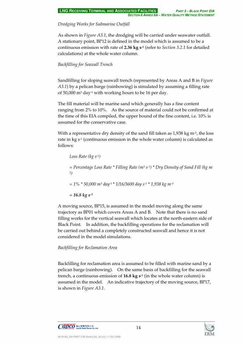
3.2.2 Trailing Suction Hopper Dredgers

Trailing Suction Hopper Dredgers (TSHD) will be used mainly for the

navigation channels and turning circle.

The hopper dry density for a TSHD is typically 0.75 ton m-3. TSHD could

dredge at a faster rate than grab dredgers (typical dredging rate of 5,400 m3

per trip per TSHD with a maximum dredging rate up to 7,200 m3 per trip

depending on the vessel size).

For the modelling scenarios it has been assumed that the Contractor will

utilise a small (<5,000 m3) to medium (5,000 – 10,000 m3) TSHD. The

suggested size of trailer dredger is approximately 8,000 m3, which commonly

operate in Hong Kong.

The rate of loss for trailer dredgers is 7 kg m-3 dredged which is considered to

be a conservative assumption and at the upper end of measured loss rates for

TSHD (1) (2), and assumes that no overflow is permitted but the Lean Mixture

Overboard (LMOB) system is in operation at the beginning and end of the

dredging cycle when the drag head is being lowered and raised from the

seabed. Assuming that no more than one dredger operates simultaneously

and the loading time for each dredging trip is approximately 0.75 hour a loss

rate (in kg s-1) is calculated as follows:

Loss Rate (kg s-1)

= Dredging Rate Per Trip (m3 s-1) * Loss Rate (kg m-3)

= 7,200 m3 trip -1 / 0.75 hr / 3600 s hr-1 * 7 kg m-3

= 18.67 kg s-1

For the THSD working at Black Point the modelling has assumed that the

trailer will dispose at the South Cheung Chau which would introduce the

travelling time to and from the site to be 3.32 hours and a cycle time would be

approximately 5.32 hours. This would equate to 3 trips per day, which

means a daily dredging rate of 21,600 m3 day-1 (3).

During dredging the drag head will sink below the level of the surrounding

seabed and the seabed sediments will be extracted from the base of the trench

formed by the passage of the draghead. The main source of sediment release

is the bulldozing effect of the draghead when it is immersed in the mud.

This mechanism means that sediment is lost to suspension very close to the

(1) Kirby, R and Land J M (1991). The impact of Dredging - A Comparison of Natural and Man-Made Disturbances to

Cohesive Sedimentary Regimes. Proceedings CEDA-PIANC Conference (incorporating CEDA Dredging Days),

November 1991, Amsterdam. Central Dredging Association, the Netherlands.

(2) Environment Canada (1994). Environmental Impacts of Dredging and Sediment Disposal. Les Consultants Jaques

Beraube Inc for the Technology Development Section, Environmental Protection Branch, Environment Canada,

Quebec and Ontario Branch.

(3) The maximum dredging rate for THSD per day is 21,600 m3. Three trips can be conducted per day and the

dredging rate for each trip is 7,200 m3.




13

level of the surrounding seabed and a height of 1 m has been adopted for the

initial location of sediment release in the model.

3.3 CONSTRUCTION SCENARIOS

3.3.1 Scenario 1a

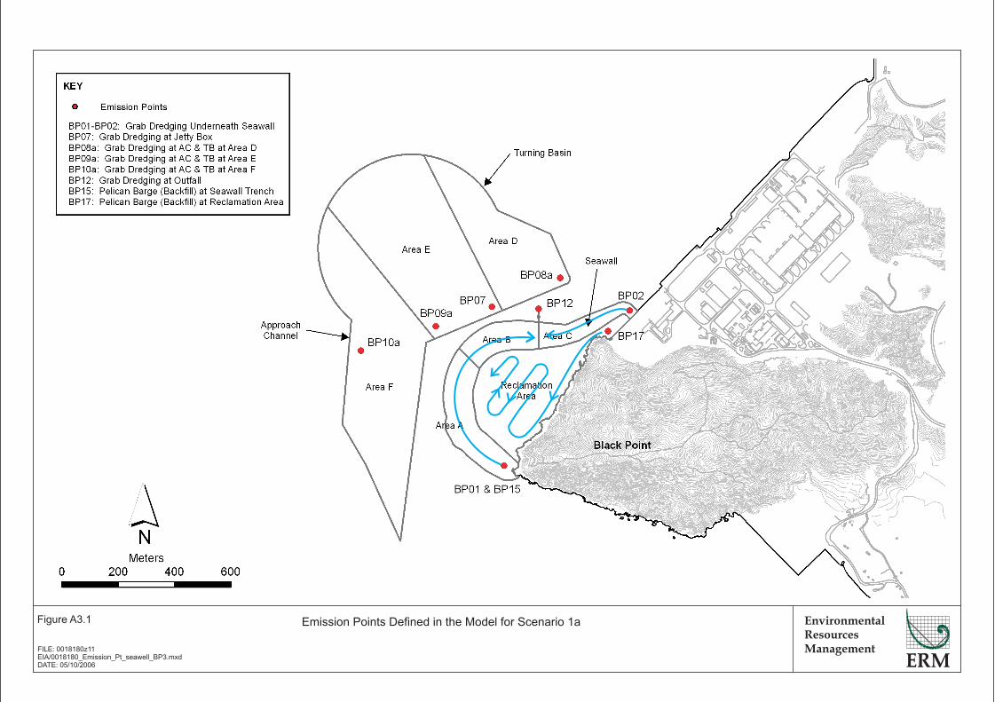
Scenario 1a simulates dredging works at seawall, jetty box, approach channel

and turning basin and outfall as well as sandfilling works for seawall trench

and reclamation (Figure A3.1). The total dredged volume is approximately

3.15 Mm3. All dredging works will be carried out by grab dredgers while

sandfilling works is conducted by a pelican barge.

Dredging Works for Seawall Areas

It is estimated that dredged volume under the seawall is approximately 0.63

Mm3. Two grab dredgers in total will be used for the construction, starting

from each end of the seawall in reverse direction. Hence in the water quality

model two moving emission sources, BP01 and BP02, initially locate at the

ends of dredging underneath seawall in Area A and Area C respectively,

moving towards Area B (Figure A3.1). All the releases are continuously

emitted in the whole water column with an emission rate of 2.36 kg s-1 (refer to

Section 3.2.1 for detailed calculations).

Dredging Works for Jetty Box, Approach Channel and Turning Basin

The estimated dredged volume along the approach channel/turning basin

and berthing area is approximately 2.52 Mm3 in total. Figure A3.1 shows the

dredging area of the approach channel and turning basin which is divided

into three areas, namely Area D, Area E and Area F. A jetty box which is

inside Area E will be dredged as well.

Three stationary sources, BP08a, BP09a and BP10a, are assumed in the model

to represent the grab dredgers in Areas D, E and F respectively and another

stationary source, BP07, represents a grab dredger at the jetty box. The most

conservative case is simulated as making the four sources close to other

sources. In reality, the grab dredgers will move away from each other and

will not retain this proximity to others for a period as long as modelled. In

addition, the dredging works at jetty box may be conducted before dredging

for Area E and thus concurrent dredging for jetty box and Area E is unlikely

to occur.

All the releases are continuously emitted in the whole water column with an

emission rate of 2.36 kg s-1 (refer to Section 3.2.1 for detailed calculations).

EnvironmentalResourcesManagement

Figure A3.1

EIA/0018180_Emission_Pt_seawell_BP3.mxdDATE: 05/10/2006

Emission Points Defined in the Model for Scenario 1a

FILE: 0018180z11




14

Dredging Works for Submarine Outfall

As shown in Figure A3.1, the dredging will be carried under seawater outfall.

A stationary point, BP12 is defined in the model which is assumed to be a

continuous emission with rate of 2.36 kg s-1 (refer to Section 3.2.1 for detailed

calculations) at the whole water column.

Backfilling for Seawall Trench

Sandfilling for sloping seawall trench (represented by Areas A and B in Figure

A3.1) by a pelican barge (rainbowing) is simulated by assuming a filling rate

of 50,000 m3 day-1 with working hours to be 16 per day.

The fill material will be marine sand which generally has a fine content

ranging from 2% to 10%. As the source of material could not be confirmed at

the time of this EIA compiled, the upper bound of the fine content, i.e. 10% is

assumed for the conservative case.

With a representative dry density of the sand fill taken as 1,938 kg m-3, the loss

rate in kg s-1 (continuous emission in the whole water column) is calculated as

follows:

Loss Rate (kg s-1)

= Percentage Loss Rate * Filling Rate (m3 s-1) * Dry Density of Sand Fill (kg m-

3)

= 1% * 50,000 m3 day-1 * 1/16/3600 day s-1 * 1,938 kg m-3

= 16.8 kg s-1

A moving source, BP15, is assumed in the model moving along the same

trajectory as BP01 which covers Areas A and B. Note that there is no sand

filling works for the vertical seawall which locates at the north-eastern side of

Black Point. In addition, the backfilling operations for the reclamation will

be carried out behind a completely constructed seawall and hence it is not

considered in the model simulations.

Backfilling for Reclamation Area

Backfilling for reclamation area is assumed to be filled with marine sand by a

pelican barge (rainbowing). On the same basis of backfilling for the seawall

trench, a continuous emission of 16.8 kg s-1 (in the whole water column) is

assumed in the model. An indicative trajectory of the moving source, BP17,

is shown in Figure A3.1.




15

3.3.2 Scenario 1b

Scenario 1b simulates the same construction activities as those modelled in

Scenario 1a. The difference between Scenario 1b and 1a is a TSHD will be

used for dredging at an area of approach channel and turning basin (Area D

shown in Figure A3.2).

As indicated in Figure A3.2, the approach channel and turning basin will be

divided into four areas, Areas D, E, F and G. Area D is proposed to be

dredged by a TSHD whereas Areas E to G will be dredged by a grab dredger.

For each trip travelled by the TSHD, the loss rate will be 18.67 kg s-1 (refer to

Section 3.2.2 for detailed calculations).

A moving source, BP08b, is assumed in the model and it will start at the

utmost south of the area and move at a speed of 0.3 m s-1 in north-eastern

direction following the angle of the approach channel. In order to account

for the disposal events as aforementioned in Section 3.2.2, the emission is

assumed to be instantaneous with a 0.75 hour dredging followed by 1.25-hour

on-site idle time and a 3.32-hour disposal whereas disposal will be at South

Cheung Chau.

3.3.3 Construction Programme and Sequence

Tentative construction programme and indicative construction sequence are

shown in Figures A3.3 and A3.4 respectively.


Figure A3.2

EIA/0018180_Emission_Pt_Approach-channel_BP_Scen1b.mxdDATE: 05/10/2006

Emission Points Defined in the Model for Scenario 1b

FILE: 0018180z12




16

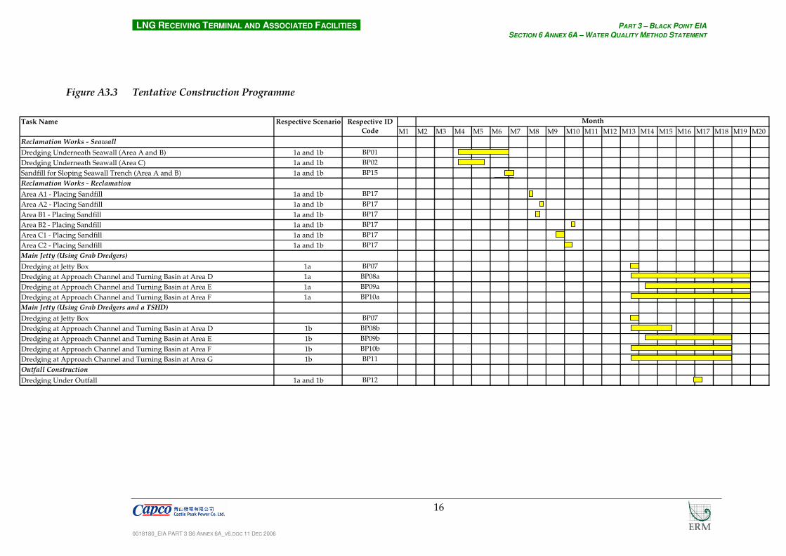
Figure A3.3 Tentative Construction Programme

M1 M2 M3 M4 M5 M6 M7 M8 M9 M10 M11 M12 M13 M14 M15 M16 M17 M18 M19 M20

Reclamation Works - Seawall

Dredging Underneath Seawall (Area A and B) 1a and 1b BP01

Dredging Underneath Seawall (Area C) 1a and 1b BP02

Sandfill for Sloping Seawall Trench (Area A and B) 1a and 1b BP15

Reclamation Works - Reclamation

Area A1 - Placing Sandfill 1a and 1b BP17

Area A2 - Placing Sandfill 1a and 1b BP17

Area B1 - Placing Sandfill 1a and 1b BP17

Area B2 - Placing Sandfill 1a and 1b BP17

Area C1 - Placing Sandfill 1a and 1b BP17

Area C2 - Placing Sandfill 1a and 1b BP17

Main Jetty (Using Grab Dredgers)

Dredging at Jetty Box 1a BP07

Dredging at Approach Channel and Turning Basin at Area D 1a BP08a

Dredging at Approach Channel and Turning Basin at Area E 1a BP09a

Dredging at Approach Channel and Turning Basin at Area F 1a BP10a

Main Jetty (Using Grab Dredgers and a TSHD)

Dredging at Jetty Box BP07

Dredging at Approach Channel and Turning Basin at Area D 1b BP08b

Dredging at Approach Channel and Turning Basin at Area E 1b BP09b

Dredging at Approach Channel and Turning Basin at Area F 1b BP10b

Dredging at Approach Channel and Turning Basin at Area G 1b BP11

Outfall Construction

Dredging Under Outfall 1a and 1b BP12

MonthRespective Scenario Respective ID

Code

Task Name


Figure A3.4

FILE: 0018180z9DATE: 05/10/2006

Black Point Indicative Construction Sequence




17

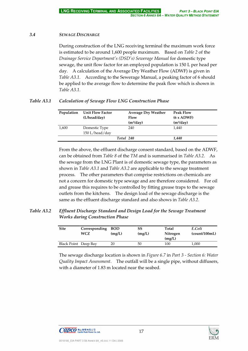
3.4 SEWAGE DISCHARGE

During construction of the LNG receiving terminal the maximum work force

is estimated to be around 1,600 people maximum. Based on Table 2 of the

Drainage Service Department’s (DSD’s) Sewerage Manual for domestic type

sewage, the unit flow factor for an employed population is 150 L per head per

day. A calculation of the Average Dry Weather Flow (ADWF) is given in

Table A3.1. According to the Sewerage Manual, a peaking factor of 6 should

be applied to the average flow to determine the peak flow which is shown in

Table A3.1.

Table A3.1 Calculation of Sewage Flow LNG Construction Phase

Population Unit Flow Factor

(L/head/day)

Average Dry Weather

Flow

(m3/day)

Peak Flow

(6 x ADWF)

(m3/day)

1,600 Domestic Type

150 L/head/day

240 1,440

Total 240 1,440

From the above, the effluent discharge consent standard, based on the ADWF,

can be obtained from Table 8 of the TM and is summarised in Table A3.2. As

the sewage from the LNG Plant is of domestic sewage type, the parameters as

shown in Table A3.1 and Table A3.2 are applicable to the sewage treatment

process. The other parameters that comprise restrictions on chemicals are

not a concern for domestic type sewage and are therefore considered. For oil

and grease this requires to be controlled by fitting grease traps to the sewage

outlets from the kitchens. The design load of the sewage discharge is the

same as the effluent discharge standard and also shows in Table A3.2.

Table A3.2 Effluent Discharge Standard and Design Load for the Sewage Treatment

Works during Construction Phase

Site Corresponding

WCZ

BOD

(mg/L)

SS

(mg/L)

Total

Nitrogen

(mg/L)

E.Coli

(count/100mL)

Black Point Deep Bay 20 50 100 1,000

The sewage discharge location is shown in Figure 6.7 in Part 3 - Section 6: Water

Quality Impact Assessment. The outfall will be a single pipe, without diffusers,

with a diameter of 1.83 m located near the seabed.




18

4 OPERATIONAL PHASE

For the study of operational effects, the approach requires several steps:

1) Running a near-field model (i.e., CORMIX) for the operational discharges,

and any existing discharges in the vicinity (eg Black Point Power Station

discharge) to characterise the initial mixing of the effluent discharge.

The results of the near-field model has been used to define the manner in

which the discharge would be included in the far-field hydrodynamic and

the water quality models (at which depth, the number of cells over which

the discharge will be distributed). The results from the CORMIX

analysis has also provided information of the near field dispersion and

dilution of the effluent plumes and hence chlorine and/or other biocide

concentrations.

Details of CORMIX simulation is presented in Appendix 6B in this Annex.

2) Adapting the hydrodynamic model for the new conditions, including the

reclamations and discharges.

3) Running the hydrodynamic model for the specified conditions (wet/dry

season). Both sites can be implemented within one hydrodynamic run

for a dry and wet seasons spring-neap cycle, since there will be no

significant interaction between the effects of the two sites.

4) Running the water quality model (i.e., Delft3D-WAQ). The objectives

are twofold:

a) to qualitatively assess the concentrations of residual chlorine or other

biocides: to this end up to 5 decayable tracers may be defined, which

will be released from the two candidate sites (the analysis has been

carried out assuming that the background concentration is zero); and

b) to qualitatively assess the potential changes in water quality as a

result of changes in the circulation near the project sites: to this end

up to 5 conservative, ie non-decayable, tracers have been defined,

which will be discharged from a number of locations representing

main pollution sources (e.g. Hong Kong as a whole, major point

sources in the vicinity of the candidate sites).

The general water quality is the result of transport phenomena and

transformation and retention processes. The operation of the project may

locally affect the transport patterns. Transformation and retention processes

are not affected. Consequently, validation of the Delft3D-WAQ model is not

required. The analysis under 4b) requires the running of a baseline scenario

to assess the pre-project conditions.




19

4.1 THERMAL AND ANTIFOULANT DISCHARGE

Stored LNG will need to be re-gasified in order for it to be conveyed along the

gas pipeline to the point of use. This will be accomplished via LNG

Vaporisers, which will either utilise piped seawater (in open rack vaporisers)

or hot combustion gases (in so-called submerged combined vaporisers) to

raise the temperature of the LNG to ambient, thereby causing it to re-gasify.

Once vaporised the LNG gas is then regulated for pressure and piped to the

consumer (1).

• Open Rack Vaporisers - In open-rack vaporisers (ORVs) downward

seawater flows over the exterior of the vaporizer panels, which internally

channel an upward flow of high-pressure LNG. LNG will then be

vaporized by exchanging heat with seawater in the ORV’s. The seawater

falls over the panels to a trough below and is then discharged back to the

sea. The seawater will pass through a series of screens to remove debris

to prevent blockage or damage to the seawater pumps. Upon leaving

the vaporisers, the (cooled) seawater will be collected in a sump and

discharged back to the sea via a submarine outfall. The design seawater

temperature drop is 12.5°C at the discharge point.

• Submerged Combined Vaporisers - In Submerged Combined Vaporisers

(SCVs), LNG flows through tubes that are submerged in a heated water

bath.

The present design intention for the terminal is that the gas will be vaporised

using ORV, with a SCV unit as back-up.

The seawater discharge is expected to have a decreased temperature of

approximate ∆ 12.5°C at the discharge point. The flow rate is expected to be

equivalent to 18,000 m3 hr-1 (peak flow).

The dosing level of Chlorine is expected to be at approximately 3 mg L-1.

Residual Chlorine level is expected to be 0.3 mg L-1. Residual chlorine is

known to decay rapidly in the marine environment, as the chlorine demand of

the receiving waters is likely to be high. A preliminary review of literature

on chlorine decay has indicated that there are a number of factors that

determine decay, including reactivity of organic matter, temperature, (UV)

light, pH and salinity. However, chlorine decay has been studied mostly for

freshwater systems and in distribution system. The discharge of residual

chlorine has been modelled based on both the peak flow of 18,000 m3 hr-1 and

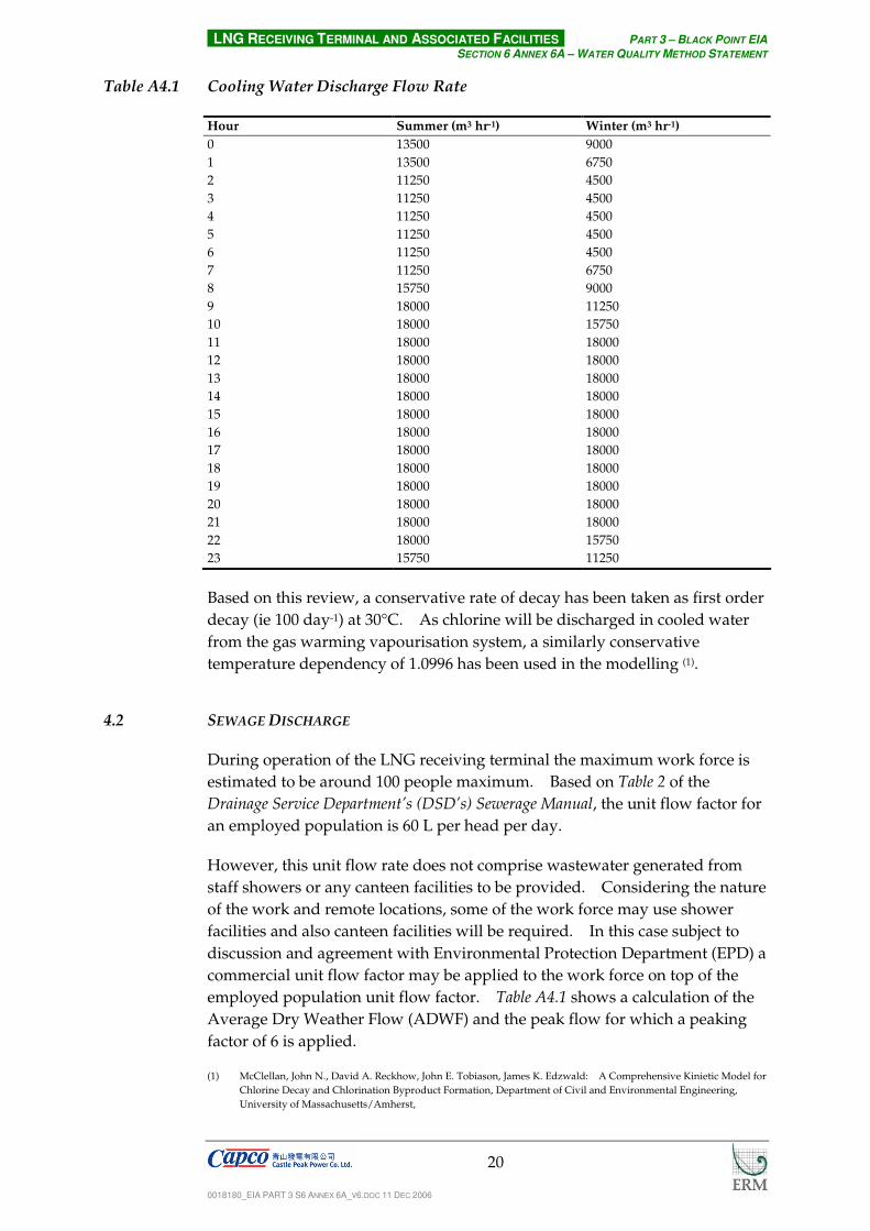
the seasonal varied flow as shown in Table A4.1.

(1) The LNG terminal is assumed to connect to the Black Point Power Station. Should the site location require a subsea

pipeline to Black Point, the pipeline will be installed in accordance with the Marine Department and Civil

Engineering Department’s requirements.




20

Table A4.1 Cooling Water Discharge Flow Rate

Hour Summer (m3 hr-1) Winter (m3 hr-1)

0 13500 9000

1 13500 6750

2 11250 4500

3 11250 4500

4 11250 4500

5 11250 4500

6 11250 4500

7 11250 6750

8 15750 9000

9 18000 11250

10 18000 15750

11 18000 18000

12 18000 18000

13 18000 18000

14 18000 18000

15 18000 18000

16 18000 18000

17 18000 18000

18 18000 18000

19 18000 18000

20 18000 18000

21 18000 18000

22 18000 15750

23 15750 11250

Based on this review, a conservative rate of decay has been taken as first order

decay (ie 100 day-1) at 30°C. As chlorine will be discharged in cooled water

from the gas warming vapourisation system, a similarly conservative

temperature dependency of 1.0996 has been used in the modelling (1).

4.2 SEWAGE DISCHARGE

During operation of the LNG receiving terminal the maximum work force is

estimated to be around 100 people maximum. Based on Table 2 of the

Drainage Service Department’s (DSD’s) Sewerage Manual, the unit flow factor for

an employed population is 60 L per head per day.

However, this unit flow rate does not comprise wastewater generated from

staff showers or any canteen facilities to be provided. Considering the nature

of the work and remote locations, some of the work force may use shower

facilities and also canteen facilities will be required. In this case subject to

discussion and agreement with Environmental Protection Department (EPD) a

commercial unit flow factor may be applied to the work force on top of the

employed population unit flow factor. Table A4.1 shows a calculation of the

Average Dry Weather Flow (ADWF) and the peak flow for which a peaking

factor of 6 is applied.

(1) McClellan, John N., David A. Reckhow, John E. Tobiason, James K. Edzwald: A Comprehensive Kinietic Model for

Chlorine Decay and Chlorination Byproduct Formation, Department of Civil and Environmental Engineering,

University of Massachusetts/Amherst,




21

Table A4.1 Calculation of Sewage Flow LNG Operational Phase

Population Unit Flow Factor

(L/head/day)

Average Dry Weather

Flow

(m3/day)

Peak Flow

(6 x ADWF)

(m3/day)

100 Employed Population

60L/head/day

6.0 36.0

100 Commercial Activities 29.0 174.0

Total 35.0 210.0

From the above, the effluent discharge standard, based on the ADWF, can be

obtained from Table 8 of the TM and is summarised in Table A4.2. As the

sewage from the LNG Plant is of domestic sewage type, the parameters as

shown in Table A4.1 and Table A4.2 are applicable to the sewage treatment

process. The other parameters that comprise restrictions on chemicals are

not a concern for domestic type sewage and are therefore considered. For oil

and grease this requires to be controlled by fitting grease traps to the sewage

outlets from the kitchens. The design load of the sewage discharge is

decided to be same as the effluent discharge standard (Table A4.2).

Table A4.2 Effluent Discharge Standard and Design Load for the Sewage Treatment

Works during Operational Phase

Site Corresponding

WCZ

BOD

(mg/L)

SS

(mg/L)

Total

Nitrogen

(mg/L)

E.Coli

(count/100mL)

Black Point Deep Bay 20 50 100 1,000

The sewage discharge location is shown in Figure 6.7 in Part 3 - Section 6: Water

Quality Impact Assessment. The outfall will be a single pipe, without diffusers,

with a diameter of 1.83 m located near the seabed.

4.3 MAINTENANCE DREDGING

The study has considered the following three steps that steer sedimentation.

Two types of material have been taken into account, i.e. mud (cohesive) and

sand (non-cohesive). Mud is transported in suspension and sand is

transported as suspended load or bed load, depending on the grain size and

wave/current conditions.

1) To estimate the rate of sediment supply, data on bed composition in the

vicinity of the LNG terminals (if available also sediment cores), data on

suspended sediment concentration (preferably also during or just after

typhoons) and data on the sediment load and the extent of the sediment

transport of Pearl River has been analysed. From the mineralogical

composition, sediment sources can be identified.

http://www.ecs.umass.edu/cee/reckhow/publ/84/acschapter/html




22

2) The current velocity in and around the navigation channel and the

resulting bed shear stress. To this end, results from existing

hydrodynamic model simulations can be used.

• The influence of waves has been evaluated based on a combination of

wave climate data analysis from measurements, existing wave model

results and desk analysis.

• An analysis of recirculation patterns by wind and tide to identify

transport pathways. The tidal excursion length is also an important

parameter to consider.

• Based on available data, it has been assessed what the effect of

seasonal variations is and what the importance of density-driven

effects is, e.g. salinity, fluid mud, temperature.

3) From the analysis on sediment supply and transport, an estimate can be

made on the sedimentation rate in the navigation channel and in the

neighbourhood of the terminal. From the average and maximum shear

stress in the trench induced by currents and waves, the sediment trapping

efficiency can be estimated. The product of supply and trapping

efficiency yields the sedimentation rate.

Following the above approach, the frequency of the maintenance dredging has

been estimated. For the impact assessment of the maintenance dredging, the

qualitative assessment has been conducted (discussed in the Section 6 – Water

Quality Impact Assessment) since the scale of the maintenance dredging would

be much less than the dredging works for the approach channel and turning

basin during construction phase which has been modelled as described in the

previous section.

4.4 ACCIDENTAL FUEL SPILLAGE

4.4.1 Locations

A release point (808583 easting, 825632 northing) is defined. A spill

occurring along the Urmston Road prior to reaching the Black Point site is

assumed in the model. This location is selected due to its proximity to CPPS

and also the Marine Park at Lung Kwu Chau/Sha Chau.

4.4.2 Fuel Type

Based on the information, it is assumed that the fuel is Heavy Fuel Oil (HFO

i.e., 100% No 6).




23

4.4.3 Volume to be spilled

The most conservative case scenario was modelled, i.e. the largest single HFO

storage tank from a 210 km3 SSD propulsion vessel which is 5,043 m3. The

inventory released should equate to 60% of the tank contents.

4.4.4 Discharge Rate

It is assumed the large carrier will be used and its large collision event has a

release rate of 8,060 kg s-1, even though the small carrier will also be adopted

in reality, giving a large collision event having a lower release rate of 7,720 kg

s-1.

4.4.5 Model Selection

The oil spillage has been simulated using hydrodynamic and particle tracking

models (oil module of Delft3D-PART) to assess the movement of the oil spill.

This Delft3D-PART forms part of the well-calibrated Delft 3D suite of models,

as described in Section 1 of this Annex. This particle tracking model has been

adopted in the EIA of Permanent Aviation Fuel Facility (1).

4.4.6 Key Modelling Assumptions

Fuel spill is modelled by surface particles (floating since the density of the oil

is less than that of the water). The initial radius is calculated on the basis of

the Fay and Hoult equation (2) that calculates the extent of the patch after

gravitational spreading. This spreading occurs in a matter of minutes rather

than hours. The radius is related to the density difference between the oil

and the water and the volume of spilled oil). The spill as used in the present

case, of heavy fuel oil would lead to an initial patch of a diameter of 440 m.

This implies a thickness of about 5 mm. In addition, no evaporation rate and

emulsification is assumed in the model. The wind data at Cheung Chau and

Sha Chau as shown in Annex 13A3 in Section 13 is used in the model.

4.4.7 Scenarios

The PART model has been simulated for the dry and wet seasons with typical

real time wind time series. The simulations were run for periods of 5 days to

capture the transport route of the oil spill in the first 24 hours to facilitate the

development of an emergency contingency plan.

(1) Mouchel Asia Ltd (2002). EIA of Permanent Aviation Fuel Facility. For Airport Authority Hong Kong. Final Report.

(2) Fay, J. and D. Hoult, 1971. Physical processes in the spread of oil on a water surface, Report DOT-CG-01 381-A, U.S.

Coast Guard, Washington, D.C.




24

5 CUMULATIVE IMPACTS

At present there are no committed projects that could have cumulative

impacts with the construction of the terminal at Black Point. No projects are

planned to be constructed in sufficient proximity to the Project to cause

cumulative effects and hence, cumulative impacts are not expected to occur.




25

6 INPUT PARAMETERS

6.1 SEDIMENT PARAMETERS

For simulating sediment impacts the following general parameters has been

used:

Settling velocity – 0.5 mm s-1

Critical shear stress for deposition – 0.2 N m-2

Critical shear stress for erosion – 0.3 N m-2

Minimum depth where deposition allowed – 1 m

Resuspension rate – 30 g m-2 d-1

Wave calculation method – Tamminga

Chezy calculation method – White/Colebrook

Bottom roughness – 0.001 m (1)

Fetch for wave driven erosion – 35 km

Depth gradient effect on waves – absent

The above parameters have been used to simulate the impacts from sediment

plumes in Hong Kong associated with uncontaminated mud disposal into the

Brothers MBA (2) and dredging for the Permanent Aviation Fuel Facility at Sha

Chau (3). The critical shear stress values for erosion and deposition were

determined by laboratory testing of a large sample of marine mud from Hong

Kong as part of the original WAHMO studies associated with the new airport

at Chek Lap Kok.

(1) The particular formulations used express the bottom roughness by the so-called Nikuradse roughness coefficient,

which has the dimension m. (Nikuradse, J., 1932: Gesetzmassigkeiten der turbulenten Stromungen in glatten

Rohren. Frosch. Ver. Deutscher Ing. No. 356.)

(2) Mouchel (2002a). Environmental Assessment Study for Backfilling of Marine Borrow Pits at North of the Brothers.

Environmental Assessment Report.

(3) Mouchel (2002b). Permanent Aviation Fuel Facility. EIA Report. Environmental Permit EP-139/2002.




26

7 SCENARIOS

7.1 CONSTRUCTION PHASE

The scenarios are constructed in accordance with the tentative construction

programme (Figure A3.3). To simulate conservative worse cases, all the

potential concurrent activities would be simulated at the same time regardless

the reality that they may not all occur simultaneously.

The proposed scenarios for the construction phase of the Black Point Option

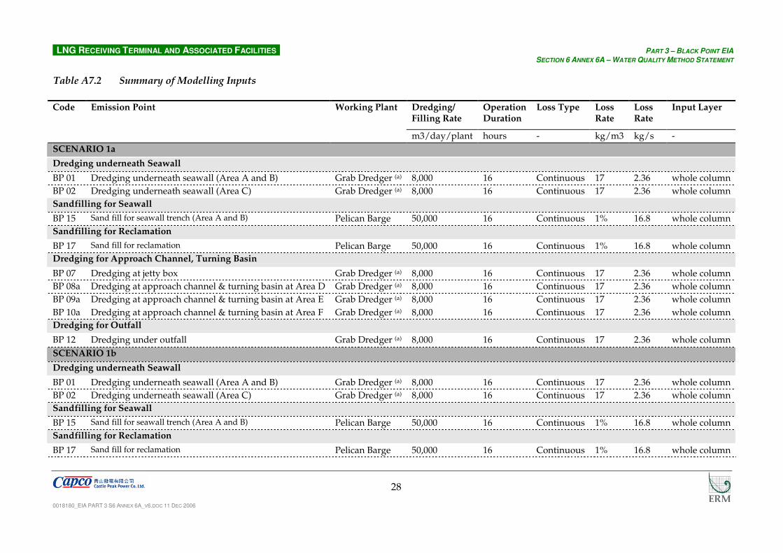
are presented in Table A7.1. Table A7.2 summarises the inputs defined in the

water quality model.

Table A7.1 Scenarios of the Construction Works for Black Point Option

Scenario ID (report)

Tasks Details of

Construction Activities

No. of Plant and

Plant Type

Code

Scenario 1a Seawall

Dredging underneath seawall (Area A and B)

1 no. Grab Dredger

BP 01

Seawall

Dredging underneath seawall (Area C)

1 no. Grab Dredger

BP 02

Seawall Sand fill for seawall trench (Area A and B)

1 no. Pelican Barge

BP 15

Reclamation Sand fill for reclamation area

1 no. Pelican Barge

BP 17

Jetty Box Grab Dredging at Jetty Box

1 no. Grab Dredger

BP 07

Approach Channel and Turning Basin

Grab Dredging at Approach Channel & TB at Area D

1 no. Grab Dredger

BP 08a


Grab Dredging at Approach Channel & TB at Area E

1 no. Grab Dredger

BP 09a


Grab Dredging at Approach Channel & TB at Area F

1 no. Grab Dredger

BP 10a

Cooled Water Outfall Grab Dredging under outfall

1 no. Grab Dredger

BP 12

Scenario 1b Seawall

Dredging underneath seawall (Area A)

1 no. Grab Dredger

BP 01

Seawall Dredging underneath seawall (Area

1 no. Grab Dredger BP 02




27

Scenario ID (report)

Tasks Details of

Construction Activities

No. of Plant and

Plant Type

Code

C)

Seawall Sand fill for seawall trench (Area A and B)

1 no. Pelican Barge

BP 15

Reclamation Sand fill for reclamation area

1 no. Pelican Barge

BP 17

Jetty Box Grab Dredging at Jetty Box

1 no. Grab Dredger

BP 07


TSHD Dredging at Approach Channel & TB at Area D

1 no. TSHD

BP 08b


Grab Dredging at Approach Channel & TB at Area E

1 no. Grab Dredger

BP 09b


Grab Dredging at Approach Channel & TB at Area F

1 no. Grab Dredger

BP 10b


Grab Dredging at Approach Channel & TB at Area G

1 no. Grab Dredger

BP 11

Cooled Water Outfall Grab Dredging under outfall

1 no. Grab Dredger

BP 12




28

Table A7.2 Summary of Modelling Inputs

Code Emission Point Working Plant Dredging/ Filling Rate

Operation Duration

Loss Type Loss Rate

Loss Rate

Input Layer

m3/day/plant hours - kg/m3 kg/s -

SCENARIO 1a

Dredging underneath Seawall

BP 01 Dredging underneath seawall (Area A and B) Grab Dredger (a) 8,000 16 Continuous 17 2.36 whole column

BP 02 Dredging underneath seawall (Area C) Grab Dredger (a) 8,000 16 Continuous 17 2.36 whole column

Sandfilling for Seawall

BP 15 Sand fill for seawall trench (Area A and B) Pelican Barge 50,000 16 Continuous 1% 16.8 whole column

Sandfilling for Reclamation

BP 17 Sand fill for reclamation Pelican Barge 50,000 16 Continuous 1% 16.8 whole column

Dredging for Approach Channel, Turning Basin

BP 07 Dredging at jetty box Grab Dredger (a) 8,000 16 Continuous 17 2.36 whole column

BP 08a Dredging at approach channel & turning basin at Area D Grab Dredger (a) 8,000 16 Continuous 17 2.36 whole column

BP 09a Dredging at approach channel & turning basin at Area E Grab Dredger (a) 8,000 16 Continuous 17 2.36 whole column

BP 10a Dredging at approach channel & turning basin at Area F Grab Dredger (a) 8,000 16 Continuous 17 2.36 whole column

Dredging for Outfall

BP 12 Dredging under outfall Grab Dredger (a) 8,000 16 Continuous 17 2.36 whole column

SCENARIO 1b

Dredging underneath Seawall

BP 01 Dredging underneath seawall (Area A and B) Grab Dredger (a) 8,000 16 Continuous 17 2.36 whole column

BP 02 Dredging underneath seawall (Area C) Grab Dredger (a) 8,000 16 Continuous 17 2.36 whole column

Sandfilling for Seawall

BP 15 Sand fill for seawall trench (Area A and B) Pelican Barge 50,000 16 Continuous 1% 16.8 whole column

Sandfilling for Reclamation

BP 17 Sand fill for reclamation Pelican Barge 50,000 16 Continuous 1% 16.8 whole column




29

Code Emission Point Working Plant Dredging/ Filling Rate

Operation Duration

Loss Type Loss Rate

Loss Rate

Input Layer

m3/day/plant hours - kg/m3 kg/s -

Dredging for Approach Channel, Turning Basin

BP 07 Dredging at Jetty Box Grab Dredger (a) 8,000 16 Continuous 17 2.36 whole column

BP 08b Dredging at approach channel & turning basin at Area D TSHD (b) 7,200 0.75 Piecewise 7 18.67 bed layer (c)

BP 09b Dredging at approach channel & turning basin at Area E Grab Dredger (a) 8,000 16 Continuous 17 2.36 whole column

BP 10b Dredging at approach channel & turning basin at Area F Grab Dredger (a) 8,000 16 Continuous 17 2.36 whole column

BP 11 Dredging at approach channel & turning basin at Area G Grab Dredger (a) 8,000 16 Continuous 17 2.36 whole column

Dredging for Outfall

BP 12 Dredging under outfall Grab Dredger (a) 8,000 16 Continuous 17 2.36 whole column

Notes:

(a) Grab dredger refers to closed grab dredger with a minimum grab size of 8 m3.

(b) For TSHD, with hopper capacity of 8,000 m3, the duration stated refers to the operation time per trip and each dredging event will last for around 0.8 hour.

(c) Bed layer refers to the bottom 10% of the water column.

Appendix 6A

Information on the Model

Inputs


ANNEX 6A APPENDIX 6A – INFORMATION ON THE MODEL INPUTS

CONTENTS

1 METHODOLOGY USED FOR THE GRID REFINEMENT 1

2 VERIFICATION OF THE GRID REFINEMENT 3

3 DETAILS OF HYDRODYNAMIC SIMULATIONS 6

4 DEEP BAY FLUSHING CAPACITY ASSESSMENT 7

4.1 INTRODUCTION 7 4.2 MODELLING METHODOLOGY 7 4.3 MODELLING RESULTS 9



0018180_EIA PART 3 S6 ANNEX 6A_APPENDIX 6A_V0.DOC 6 OCT 2006

1

1 METHODOLOGY USED FOR THE GRID REFINEMENT

The applied grid refinements have been realised in the Delft3D-FLOW model

by means of the so-called domain decomposition technique. The FLOW

model grid has subsequently been adopted without further aggregation in the

water quality models.

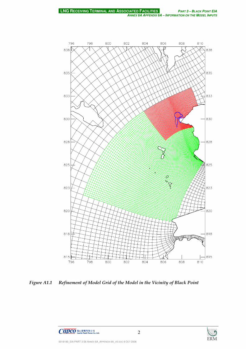
Domain decomposition is a technique in which a model domain is subdivided

into several smaller model domains, which are called sub-domains. Domain

decomposition allows for local grid refinement, both in horizontal direction

and in vertical direction. Grid refinement in horizontal direction means that

in one sub-domain smaller mesh sizes (fine grid) are used than in other sub-

domains (coarse grid) (see Figure A1.1).

The FLOW computations are carried out separately on the sub-domains. The

communication between the sub-domains takes place along internal open

boundaries, or so-called dd-boundaries. The resulting equations are solved

simultaneously for all boundaries.

In the current model, 5 horizontally refined sub-domains are distinguished.

The division in sub-domains is based on the requirements for horizontal

model resolution in order to represent the coastline and bathymetry near the

project sites and to adequately simulate physical processes.

The domain decomposition approach implemented in Delft3D-FLOW is based

on a subdivision of the domain into non-overlapping sub-domains. An

efficient iterative method is used for solving the discretised equations over the

sub-domains. A direct iterative solver is used for the continuity equation,

which is comparable to the single domain implementation. For the

momentum equations, the transport equation and the turbulence equations

the so-called additive Schwarz method is used, which allows for parallelism

over the sub-domains. Upon convergence, this type of iteration process is

comparable to the corresponding iterative solution methods in the single

domain code, and features a comparable robustness. As witnessed by

numerical experiments carried out during the development of the technique,

the differences introduced by separating domains turn out to be of

insignificance.




2

Figure A1.1 Refinement of Model Grid of the Model in the Vicinity of Black Point




3

2 VERIFICATION OF THE GRID REFINEMENT

The verification of the correct implementation of the grid refinement has been

carried out by graphically comparing the results from the original, unrefined

model with the refined model. This has been done for two locations:

• A location near the intake point of Black Point Power Station, inside the

refined domain around the Black Point site.

The results are shown in Figures A2.1 (wet season) and Figures A2.2 (dry

season). The comparison includes the water level (top graph), the current

speed (second graph), the surface and bottom salinity (third graph) and the

surface and bottom temperature (bottom graph). The comparison has been

carried out for both the wet and the dry season simulations.

The results clearly demonstrate that the overall behaviour of both models is

consistent, while the results are slightly different in the details. This is

exactly as it would be expected from a locally refined model.




4

Figure A2.1 Comparison (Wet Season) between Unrefined Model (in black) and Refined

Model (in red) at the Black Point Power Station Intake in (Top graph: Water

Level; Second graph: Current Speed; Third graph: Surface (layer 1) and Bottom (layer 10)

Salinity; and Bottom graph: Surface (layer 1) and Bottom Temperature)




5

Figure A2.2 Comparison (Dry Season) between Unrefined Model (in black) and Refined

Model (in red) at the Black Point Power Station Intake in (Top graph: Water

Level; Second graph: Current Speed; Bottom graph: Surface (layer 1) and Bottom (layer 10)

Salinity




6

3 DETAILS OF HYDRODYNAMIC SIMULATIONS

All hydrodynamic scenarios are simulated for a spring-neap-cycle during the

dry season and a spring-neap-cycle during the wet season. The simulated

periods are:

• Dry season: simulation period from 2 February 12:00h to 22 February

12:00h, simulation period 20 days, time step 30 seconds.

• Wet season: simulation period from 19 July 04:00h to 10 August 04:00h,

simulation period 22 days, time step 30 seconds.

Adequate spin-up has been provided for salinity and temperature by means of

initial conditions files (as shown by verification results). The first 5 days of

both simulation periods are also used as spin-up, and are not used for the

assessments purpose.

The wind has been set to typical seasonally averaged values:

• Dry season: northeast, 5 m s-1.

• Wet season: southwest, 5 m s-1.

The rivers have been set to typical seasonal values:

Dry (m3 s-1) Wet (m3 s-1)

Humen 1248 7442

Jiaomen 527 4732

Hongqili 128 1535

Hengmen 136 2805

Deep Bay 2.5 16




7

4 DEEP BAY FLUSHING CAPACITY ASSESSMENT

4.1 INTRODUCTION

As part of the project, one of the objectives of the modelling exercise is to

assess “any residual impacts, which include any change in hydrodynamic

regime” due to construction and operation of the LNG. In this respect, the

construction of the Black Point Terminal may affect the circulation of water in

the Deep Bay due to changes in coastline morphology, bathymetry and project

related discharges. This, in turn, may induce a change in the flushing

efficiency, and hence, in the water quality of the Deep Bay.

The objective of this study is “to assess, by modelling, the impact of the Black

Point Terminal on the flushing efficiency of the Deep Bay”.

In that respect, we propose to perform a set of tracer simulations. It is

suggested to add a tracer in the Shenzhen river discharge, and to calculate the

concentration of this tracer without the terminal (Case 1: Baseline), and with

the terminal (Case 2: Operation Phase). The simulations for both cases would

be done during neap-spring cycles in the dry and wet seasons.

4.2 MODELLING METHODOLOGY

4.2.1 Model selection

The study is based on the already existing hydrodynamic simulations using

the Delft3D hydrodynamic model (FLOW). The tracer simulations have been

done using the Delft3D water quality model (WAQ), and have used the

output from the FLOW simulations as hydrodynamic inputs into WAQ.

4.2.2 Model inputs

The study assesses the flushing capacity of Deep Bay by looking at the

concentrations inside Deep Bay as a result of a constant tracer release in

Shenzen River. When a (dynamic) equilibrium is reached, the amount of

tracer entering Deep Bay will be the same as the amount of tracer leaving

Deep Bay. The rate of flushing however will determine the tracer

concentrations inside Deep Bay: if the flushing is effective the concentrations

are low, if the flushing is not effective the concentrations are high. By

comparing the concentrations before and after the implementation of the

project it can be known whether the flushing has been affected, i.e., a

concentration increase indicates a reduction of the flushing while a

concentration decrease indicates an increased flushing.

The situation prior to the project implementation is represented by the

Baseline flow calculation, while the situation after the project implementation

is represented by the Operational flow calculation (Seasonal Varied Flow).




8

Simulations have been carried out for typical wet season and typical dry

season conditions. The duration of the run is one neap-spring cycle. The

time series output data have been acquired with a time step of 10 minutes.

The output stations are chosen as the locations of the sensitive receivers (SRs)

around Black Point (as identified in the EIA study, Part 2, Section 6: Water

Quality Impact Assessment). On top of this, a series of additional output

stations has been defined (see Figure A4.1), as well as a monitoring area to

evaluate the average tracer concentration over the whole water volume of

Inner Deep Bay (see area east of the read line, Figure A4.1).

In this exercise, the boundary conditions are set to zero with respect to the

tracer concentration. The Shenzhen River constitutes the only source of

tracer. The flow of the Shenzhen River has been attributed a constant tracer

concentration of 1 g m-3.

The simulations are given sufficient spin-up to reach a dynamic equilibrium in

the system.

Figure A4.1 Stations and area (east of red line) for time series output




9

4.3 MODELLING RESULTS

The results of the simulations are presented as a time-averaged over the last

week of the simulation (after the dynamic equilibrium has been obtained),

before and after the implementation of the project, in the dry and wet seasons,

see Table 4.1.

Table 4.1 Tracer concentration at SR’s under baseline conditions, and relative change

due to project implementation

Baseline Ope/Bas 1, 2

Dry Wet Dry Wet

Station

Concentration (mg L-1) Relative Change

Deep Bay 0.0123 0.0114 0.997 1.005

sr52-surf 0.0119 0.0132 0.998 1.024

sr45-surf 0.0128 0.0109 0.989 1.019

sr51-surf 0.0175 0.0043 1.000 1.001

sr46-surf 0.0212 0.0228 1.000 1.007

sr47-surf 0.0326 0.0240 0.999 1.010

sr50-surf 0.0532 0.0545 1.000 1.001

sr48-surf 0.1448 0.0910 1.000 1.001

sr49-surf 0.6155 0.1562 1.000 1.000

Notes:

1. Ope = Operational Flow Calculation 2. Bas = Baseline Flow Calculation

The results show that for Deep Bay as a whole there is a marginal increase of

the flushing during the dry season, indicated by a decrease of the

concentration. During the wet season there is a marginal decrease of the

flushing, indicated by an increase of the concentration.

Looking at those individual SRs which show tracer concentrations higher than

1% of the discharge concentration, it can be seen that a similar picture as for

Deep Bay as a whole: a small increase of the flushing during the dry season

and a small decrease of the flushing during the wet season. At individual

SRs the maximum concentration change is -1.1% during the dry season and

2.4% during the wet season.

From the modelling results as shown above, it is thus considered that the

change in flushing capacity due to the reclamation at outer Deep Bay is

minimal.

Appendix 6B

Information on CORMIX

Model

ENVIRONMENTAL RESOURCES MANAGEMENT

CONTENTS

1 CORMIX SIMULATIONS 1

1.1 INTRODUCTION 1 1.2 CONDITIONS AROUND THE OUTFALL LOCATIONS 1


1

1 CORMIX SIMULATIONS

1.1 INTRODUCTION

The effluent from the LNG terminal will be discharged through the outfall

located to the north of Black Point. The outfall is a single pipe with a

diameter of 1.83 m, without diffusers.

The aim of the CORMIX modelling is to determine the near field mixing

characteristics. These characteristics will be used to set the manner in which

the discharge is introduced in the 3D hydrodynamic model.

1.2 CONDITIONS AROUND THE OUTFALL LOCATIONS

From the information that was provided is derived that the outfall is located at

(807995, 830190) (Hong Kong 1980 coordinate system). The hydrodynamic

conditions were determined for the wet and dry seasons. These conditions

were taken from existing baseline computation (Tables 1.1 and 1.2).

When currents are relatively low during the wet season, the Near Field Region

(NFR) is about 100 m and for higher currents about 200 m. At the edge of the

NFR the plume has a width of the order of 5-10 m. In the wet season

calculations, the plume at the end of the NFR is in the order of 2.5-4 m thick

and is near the bottom (which is about half the total water depth). The

discharge cells are about 40 * 65 m. Hence, the discharge during the wet

season should be covering about 2 grid cells around the discharge location.

The effluent should be discharge in the lower half of the water column.

For the dry season the effluent mixes over the entire depth when currents are

higher (mid tide conditions), whilst under lower currents the effluent sinks

towards the bed and at the edge of the mixing zone the layer thickness is

about 3 m thick. The size of the plume is approximately similar to the plume

under wet season conditions. Thus the horizontal distribution of the

discharge cells may be the same for the dry as wet season conditions.


2

Table 1.1 Wet Season Conditions

Bottom -7 mPD

Neap tide Spring tide

HW LW Mid HW LW Mid

Depth (m) 9.2 7.5 8.4 9.8 7 8.4

Tbot (ºC) 25 27.5 26.5 25.5 28.4 27

Sbot (ppt) 24 14 16 22 8.5 13

ρbot (kg m-3) 1015.1 1006.9 1008.7 1013.5 1002.5 1006.3

Tsurf (ºC) 30 29.5 29.5 29 29.5 29.5

Ssurf (ppt) 2 5 5 9 5 5

ρsurf (kg m-3) 997.2 999.6 999.6 1002.7 999.6 999.6

Vbot (m s-1) 0.3 0.25 0.7 0.4 0.45 0.5

Vsurf (m s-1) 0.4 0.65 1.5 0.85 0.35 0.95

Tout (ºC) 19 20 19.5 18.75 20.45 19.75

Sout (ppt) 13 9.5 10.5 15.5 6.75 9

ρout (kg m-3) 1008.2 1005.4 1006.2 1010.2 1003.2 1005.0

Notes:

(a) “bot” denotes the bed

(b) “surf” denotes the surface

(c) “out” denotes the effluent characteristics


3

Table 1.2 Dry Season Conditions

Bottom (from model) -7 m PD

Neap tide Spring tide

HW LW Mid HW LW Mid

Depth (m) 8.8 7.6 8.2 9.6 7 8.3

Tbot (ºC) 23 23 23 23 23 23

Sbot (ppt) 28.5 29 28.5 31.5 25.5 28.5

ρbot (kg m-3) 1019.1 1019.5 1019.1 1021.4 1016.8 1019.1

Tsurf (ºC) 25 23.5 23 23.5 24 23

Ssurf (ppt) 25 26.5 25 29.5 24.5 25

ρsurf (kg m-3) 1015.9 1017.4 1016.4 1019.7 1015.8 1016.4

Vbot (m s-1) 0.15 0.1 0.4 0.1 0.3 0.9

Vsurf (m s-1) 0.4 0.2 0.9 0.35 0.5 1.5

Tout (ºC) 15.5 14.75 14.5 14.75 15 14.5

Sout (ppt) 26.75 27.75 26.75 30.5 25 26.75

ρout (kg m-3) 1019.5 1020.4 1019.7 1022.5 1018.2 1019.7

Notes:

(d) “bot” denotes the bed

(e) “surf” denotes the surface

(f) “out” denotes the effluent characteristics

Date post:	21-Mar-2018
Category:	Documents
Upload:	vothien
View:	218 times
Download:	4 times

Water Quality Method · PDF fileThis Method Statement presents information on the approach for...

Documents