Water Quality Modelingcalwater.ca.gov/.../TechnicalAppendixA_ModelingStudies.pdfTABLE OF CONTENTS A....

Water Quality Modeling Technical Appendix

Integrated Storage Investigations In-Delta Storage Feasibility Study

Draft May 2002

Delta Modeling Section Modeling Support Branch

Office of State Water Project Planning Department of Water Resources

FOREWORD The CALFED Record of Decision (ROD) has identified the In-Delta Storage Program as a potential project to be pursued for improvement in Delta water quality and enhancement of water supply flexibility. Stage 1 of the ROD requires that feasibility studies be conducted to select and recommend a project alternative by December 2001. The Office of State Water Project Planning’s Delta Modeling Section was tasked with conducting a water quality modeling evaluation of the proposed In-Delta Storage project. Modeling tasks were conducted by the Delta Modeling Section in coordination with the U.S. Bureau of Reclamation and the Department of Water Resources’ Division of Planning and Local Assistance. This technical appendix is a loose compilation of key reports and memorandums that summarize elements of the water quality modeling work that were completed in support of the In-Delta Storage Feasibility Study. Please refer to the following report for additional technical documentation on model development and validation conducted in support of the study: Methodology for Flow and Salinity Estimates in the Sacramento-San Joaquin Delta and Suisun Marsh, Twenty-Second Annual Progress Report to the State Water Resources Control Board, August 2001. Paul Hutton Chief, Delta Modeling Section

TABLE OF CONTENTS A. DSM2 Evaluation of In-Delta Storage Alternatives B. Water Quality Modeling Work Plan C. Fingerprint Evaluation of DSM2 Dissolved Organic Carbon (DOC) and

Ultraviolet Absorbance (UVA) Validation Study D. DSM2 Evaluation of Delta Wetlands Operation Study E. Running DSM2 in Planning Mode Using Daily Varying Hydrology and Non-

Repeating Tide F. Implementation of Flooded Island Water Quality Algorithm in DSM2 G. Salinity Relationships at Delta Urban Diversions H. Estimated DOC/TOC Ratios I. Boundary DOC and UVA for DSM2 Planning Studies J. Development of Flow Salinity Relationships for CALSIM K. CALSIM Water Quality Constraints to Meet Delta Wetlands WQMP L. CALSIM Water Quality Operating Rules to Meet Delta Wetlands WQMP M. Simulated DOC to Historical DICU Correlations N. DOC-UVA Correlations

OFFICE MEMO DATE:

April 18, 2002 TO:

Tara Smith

FROM: Michael Mierzwa

SUBJECT: DSM2 Evaluation of In-Delta Storage Alternatives

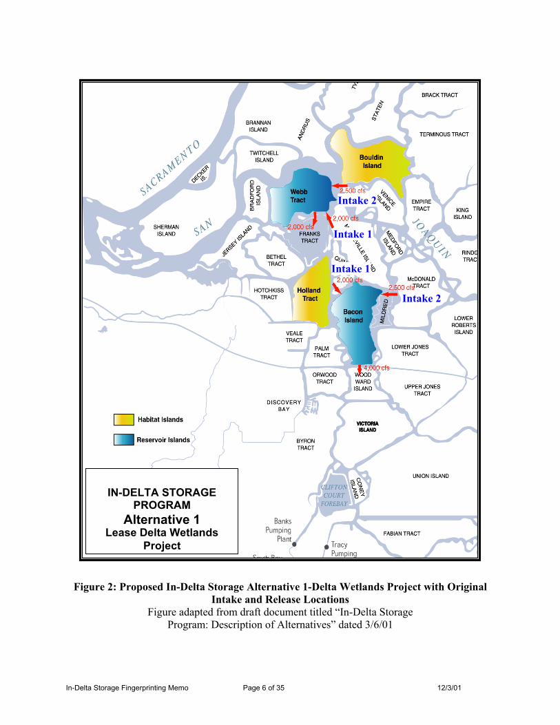
1 Introduction DWR's Integrated Storage Investigations (ISI) is reviewing the Delta Wetlands proposal to convert two Delta islands, Bacon Island and Webb Tract, into reservoirs and to restore two other Delta islands, Bouldin Island and Holland Tract, as wetland habitats. The two reservoir islands (referred to as the "project islands") would be used to store water during surplus flow periods. This surplus water would later be released for export enhancement (i.e. increases in State Water Project pumping) or to meet Delta flow/water quality requirements. ISI has re-engineered the Delta Wetlands originally proposed project, and the new ISI proposal was the basis of these DSM2 simulations. The project will be referred to as the In-Delta Storage project to distinguish it from the original Delta Wetlands proposal. Two 16-year daily hydrologies, one representing current operations (the base case) and one representing projected operations of the project islands, developed using CALSIM II were used as the input for DSM2-HYDRO and QUAL. CALSIM II also provided the releases and diversions to the project islands. The study period was from 1975 to 1991. The most recent version of the DSM2 geometry was used. The physical specification for the project islands and habitat islands were provided by ISI. A complete record of stage and EC at Martinez were used by HYDRO and QUAL respectively, and dissolved organic carbon (DOC) at the Sacramento River, San Joaquin River, Eastside stream, and Yolo Bypass boundaries were developed for use in QUAL. QUAL was modified to account for DOC increases due to storage retention based on Jung (2001a), and then used to simulate EC and DOC. This report includes the descriptions of the two scenarios and the results of these DSM2 simulations at four M&I intake locations: Contra Costa's Rock Slough intake near the Old River, Contra Costa's Los Vaqueros intake on the Old River, the State Water Project (SWP) and Central Valley Project (CVP) intakes at Banks and Tracy. Using QUAL's simulated EC and DOC, ultraviolet absorbance at 254 nm (UVA) and the formation of total trihalomethane (TTHM) and bromate at these locations were calculated. Finally, DSM2-PTM (Particle Tracking Model) was used to study the flow patterns associated with the project releases.

-1-

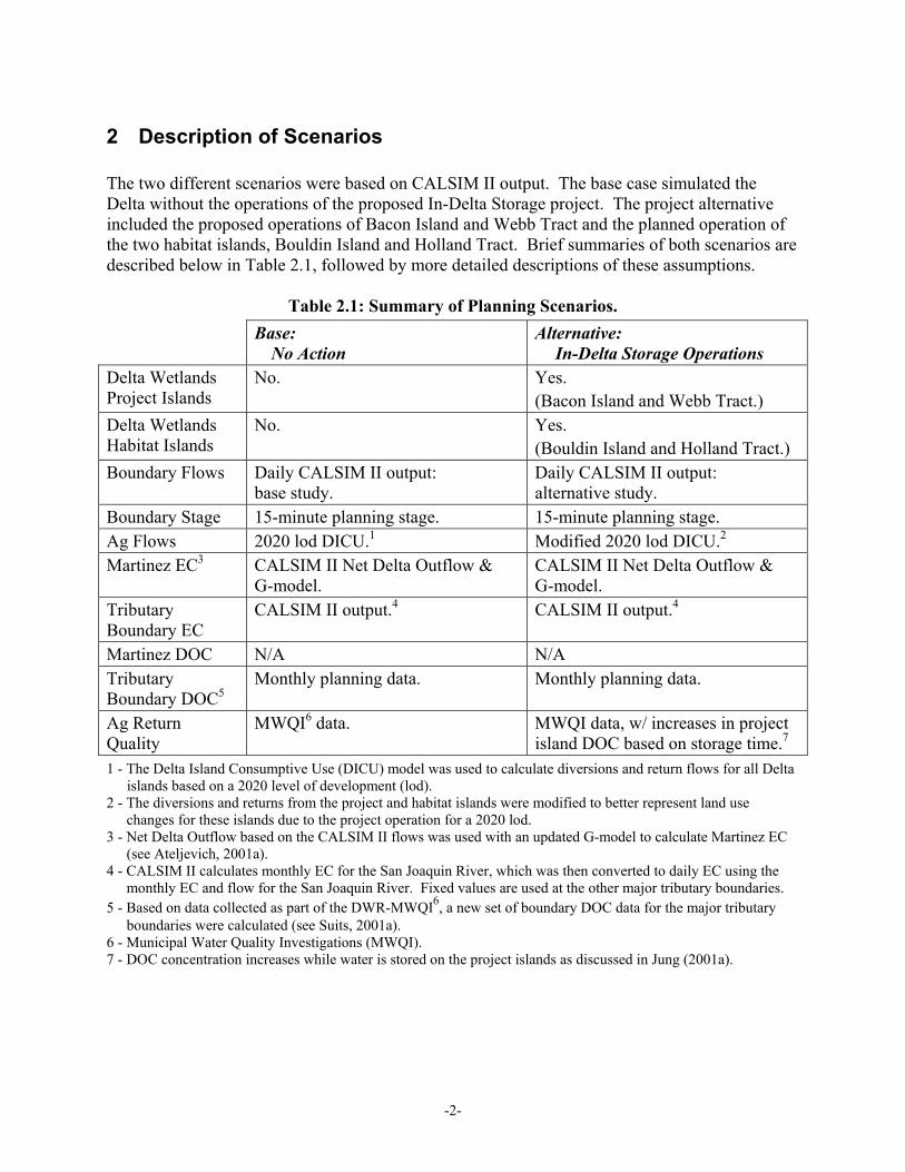
2 Description of Scenarios The two different scenarios were based on CALSIM II output. The base case simulated the Delta without the operations of the proposed In-Delta Storage project. The project alternative included the proposed operations of Bacon Island and Webb Tract and the planned operation of the two habitat islands, Bouldin Island and Holland Tract. Brief summaries of both scenarios are described below in Table 2.1, followed by more detailed descriptions of these assumptions.

Table 2.1: Summary of Planning Scenarios. Base:

No Action Alternative: In-Delta Storage Operations

Delta Wetlands Project Islands

No. Yes. (Bacon Island and Webb Tract.)

Delta Wetlands Habitat Islands

No. Yes. (Bouldin Island and Holland Tract.)

Boundary Flows Daily CALSIM II output: base study.

Daily CALSIM II output: alternative study.

Boundary Stage 15-minute planning stage. 15-minute planning stage. Ag Flows 2020 lod DICU.1 Modified 2020 lod DICU.2

Martinez EC3 CALSIM II Net Delta Outflow & G-model.

CALSIM II Net Delta Outflow & G-model.

Tributary Boundary EC

CALSIM II output.4 CALSIM II output.4

Martinez DOC N/A N/A Tributary Boundary DOC5

Monthly planning data. Monthly planning data.

Ag Return Quality

MWQI6 data. MWQI data, w/ increases in project island DOC based on storage time.7

1 - The Delta Island Consumptive Use (DICU) model was used to calculate diversions and return flows for all Delta islands based on a 2020 level of development (lod).

2 - The diversions and returns from the project and habitat islands were modified to better represent land use changes for these islands due to the project operation for a 2020 lod.

3 - Net Delta Outflow based on the CALSIM II flows was used with an updated G-model to calculate Martinez EC (see Ateljevich, 2001a).

4 - CALSIM II calculates monthly EC for the San Joaquin River, which was then converted to daily EC using the monthly EC and flow for the San Joaquin River. Fixed values are used at the other major tributary boundaries.

5 - Based on data collected as part of the DWR-MWQI6, a new set of boundary DOC data for the major tributary boundaries were calculated (see Suits, 2001a).

6 - Municipal Water Quality Investigations (MWQI). 7 - DOC concentration increases while water is stored on the project islands as discussed in Jung (2001a).

-2-

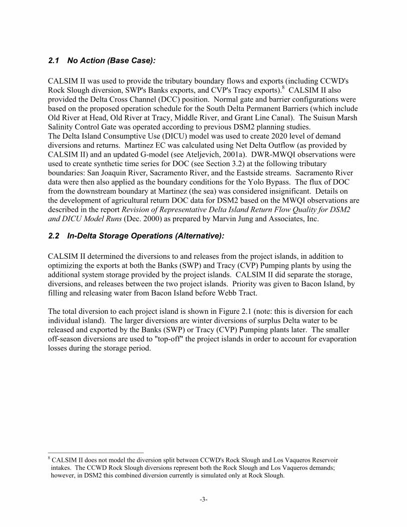
2.1 No Action (Base Case): CALSIM II was used to provide the tributary boundary flows and exports (including CCWD's Rock Slough diversion, SWP's Banks exports, and CVP's Tracy exports).8 CALSIM II also provided the Delta Cross Channel (DCC) position. Normal gate and barrier configurations were based on the proposed operation schedule for the South Delta Permanent Barriers (which include Old River at Head, Old River at Tracy, Middle River, and Grant Line Canal). The Suisun Marsh Salinity Control Gate was operated according to previous DSM2 planning studies. The Delta Island Consumptive Use (DICU) model was used to create 2020 level of demand diversions and returns. Martinez EC was calculated using Net Delta Outflow (as provided by CALSIM II) and an updated G-model (see Ateljevich, 2001a). DWR-MWQI observations were used to create synthetic time series for DOC (see Section 3.2) at the following tributary boundaries: San Joaquin River, Sacramento River, and the Eastside streams. Sacramento River data were then also applied as the boundary conditions for the Yolo Bypass. The flux of DOC from the downstream boundary at Martinez (the sea) was considered insignificant. Details on the development of agricultural return DOC data for DSM2 based on the MWQI observations are described in the report Revision of Representative Delta Island Return Flow Quality for DSM2 and DICU Model Runs (Dec. 2000) as prepared by Marvin Jung and Associates, Inc.

2.2 In-Delta Storage Operations (Alternative): CALSIM II determined the diversions to and releases from the project islands, in addition to optimizing the exports at both the Banks (SWP) and Tracy (CVP) Pumping plants by using the additional system storage provided by the project islands. CALSIM II did separate the storage, diversions, and releases between the two project islands. Priority was given to Bacon Island, by filling and releasing water from Bacon Island before Webb Tract. The total diversion to each project island is shown in Figure 2.1 (note: this is diversion for each individual island). The larger diversions are winter diversions of surplus Delta water to be released and exported by the Banks (SWP) or Tracy (CVP) Pumping plants later. The smaller off-season diversions are used to "top-off" the project islands in order to account for evaporation losses during the storage period.

8 CALSIM II does not model the diversion split between CCWD's Rock Slough and Los Vaqueros Reservoir intakes. The CCWD Rock Slough diversions represent both the Rock Slough and Los Vaqueros demands; however, in DSM2 this combined diversion currently is simulated only at Rock Slough.

-3-

Diversions to Project Islands

0

500

1000

1500

2000

Oct-75

Oct-76

Oct-77

Oct-78

Oct-79

Oct-80

Oct-81

Oct-82

Oct-83

Oct-84

Oct-85

Oct-86

Oct-87

Oct-88

Oct-89

Oct-90

Flow

(cfs

)

Bacon Island

Webb Tract

Figure 2.1: Diversions to In-Delta Storage Project Islands.

The total release from each project island is shown in Figure 2.2. Many of the summer project island releases are constrained by amount of water stored in the project islands.

Releases from Project Islands

0

500

1000

1500

2000

Oct-75

Oct-76

Oct-77

Oct-78

Oct-79

Oct-80

Oct-81

Oct-82

Oct-83

Oct-84

Oct-85

Oct-86

Oct-87

Oct-88

Oct-89

Oct-90

Flow

(cfs

)

Bacon Island

Webb Tract

Figure 2.2: Releases from In-Delta Storage Project Islands.

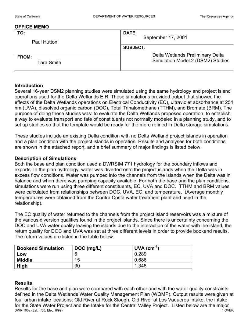
2.2.1 Project Island Configuration The configuration of the project islands as modeled by DSM2 is listed in Table 2.2. The storage capacity, surface area, discharge location, and both intake / release siphon locations for the project islands were provided by ISI. Each island is designed to use two reversible siphons to divert water onto and later off each island. The diversion and release schedules provided by CALSIM II were divided equally between each island's siphons. The location of the siphons is shown in Figures 2.3 and 2.4. The surface area of each island is fixed in DSM2. The surface area was chosen such that when full, each island would have a maximum depth of approximately 20 ft.

-4-

Table 2.2: DSM2 Configuration of Delta Wetlands Project Islands.

Island Storage Capacity (TAF)

Surface Area (acres)

Siphon #1 DSM2 Node

Siphon #2 DSM2 Node

Bacon Island 120 5,450 128 121 Webb Tract 118 5,370 40 103

Siphon #1

Bacon Island

Siphon #2

Figure 2.3: DSM2 Representation of Bacon Island.

Siphon #1

Webb Tract

Siphon #2

Figure 2.4: DSM2 Representation of Webb Tract.

The volume of water stored in each island reservoir is a direct function of the amount of water diverted into or released from each island. Volume of a reservoir in DSM2 is the product of the reservoir's surface area (listed above in Table 2.2 for the project islands) and its current stage

-5-

level. The project islands were isolated from the Delta channels, thus there was no limit to the stage in either reservoir. In order to prevent drying up of the island reservoirs an additional 0.2 ft of water was assumed to be present on both islands at the beginning of the simulation.9 This water was considered dead storage and was never released into the Delta.

2.2.2 Project Island Water Quality Water quality from the project islands was modeled two different ways using DSM2: (1) by normal mixing in order to simulate EC, and (2) by increasing the concentration of DOC in the project reservoirs as a function of time. These two different approaches are described in detail below.

EC For the QUAL EC simulations the reservoirs were isolated from the Delta channels as described in the previous section and flow between the surrounding channels and the project islands were regulated in DSM2 by using a direct "object-to-object" transfer. When water was diverted into the islands, this object-to-object transfer moved water from both of the siphons into or out of the reservoir. Project island diversions and releases were evenly split between the two siphons on each island. This process allowed QUAL to automatically mix incoming EC concentrations from the nearby channels (or an adjacent non-project reservoir) with the EC already present in the reservoirs. The EC concentration of the island reservoirs only changed when water was transferred into the islands, not when water exited the islands. This process is described in greater detail in Section 4.1.

DOC Based on work conducted by Jung (2001a), QUAL was modified for the DOC simulations such that the DOC concentration in each of the island reservoirs would increase as a function of time as described by Pandey (2001). When water was transferred into the reservoirs using the same object-to-object transfer described above, QUAL would reset the quality of the reservoir to mix with the DOC concentration of the incoming water. After this initial transfer, the DOC concentration would then increase based on Jung’s growth functions (for more details see Section 3.2.2).

2.2.3 Habitat Island Configuration In addition to modeling changes due to the operation of the project on Bacon Island and Webb Tract, changes were made in the consumptive use of Holland Tract and Bouldin Island in accordance with the plans to convert these two islands to become wetland habitats. The locations of the agricultural diversions were left unchanged for both habitat islands, but the agricultural returns on the habitat islands were moved to a single location for each island. This was done, because it was assumed that existing siphons would still be used to divert water onto the islands in order to maintain the wetland habitats, but the releases would be easier to manage 9 DSM2 can not run if a reservoir or channel becomes completely dry. This dead storage was added for the benefit of DSM2.

-6-

through a single discharge point. The DSM2 representation of Holland Tract and Bouldin Island is shown in Figures 2.5 and 2.6.

Figure 2.5: DSM2 Representation of Holland Tract.

Holland Tract

Ag Return

Bouldin Island

Ag Return

Figure 2.6: DSM2 Representation of Bouldin Island.

-7-

2.2.4 Project and Habitat Island Land Use With changes in the land use of the project islands, the diversions and return flows for the project islands were modified using the DICU model. DICU computes the consumptive use at each node in DSM2 based on historical needs for each island or water habitat in the Delta. The diversions and return flows for each island are distributed to different nodes, such that the modeled diversions, return flows, and/or seepage at any one node frequently include the individual contributions from different islands. The diversions and return flows for the project islands were removed from all of the nodes surrounding the islands (i.e. there were no agricultural diversions or return flows associated with the project islands). Monthly average consumptive use data taken from the Delta Wetlands EIR (see Figure 2.7) for the habitat islands were used to represent the water needs of the wetland habitats. The same monthly flow value was applied to both Holland Tract and Bouldin Island in each year of the simulation. The total diversions were divided equally among the siphons for each island, while as noted above, the return flow was discharged at a single location for each island.

Habitat Island Consumptive Use

0

10

20

30

40

50

60

70

Oct Nov Dec Jan Feb Mar Apr May Jun Jul Aug Sep

Flow

(cfs

)

Diversion / Applied WaterRelease / Returned Water

Figure 2.7: Monthly Habitat Island Consumptive Use

Even though the amount of water returning to the Delta from each habitat island changed each month (see Figure 2.7), the quality of this returned water was set to fixed concentrations as shown in Table 2.3. The DOC concentrations were based on return water quality observations taken on Holland Tract, Twitchell Island, and in similar wetland habitats (Jung, 2001b). The EC concentrations for the habitat islands are based on observations of the annual averages for each island.

Table 2.3: Habitat Island Return Water Quality Concentrations. Habitat Island Return EC Concentration

(umhos/cm) Return DOC Concentration

(mg/l) Bouldin Island 750 50 Holland Tract 1100 40

-8-

Since seepage in DSM2 represents the amount of water that comes from the Delta channels to the islands, it was not modified for either scenario.

3 Simulation Inputs

3.1 Hydrodynamics

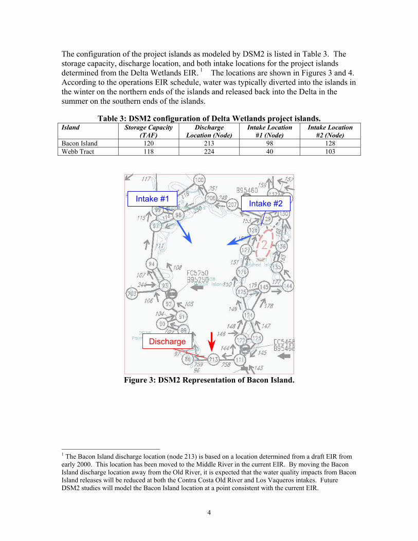
3.1.1 Flow Tributary flows, exports, and diversions were provided by CALSIM II for both the base and alternate case simulations. Similar CALSIM II studies that were used in previous DSM2 In-Delta Storage simulations are described by Easton (2001). The tributary flows include the Sacramento River, San Joaquin River, and the Yolo Bypass and one combined parameter representing the eastside flows into the Delta. Exports include the State Water Project (SWP), the Central Valley Project (CVP), Vallejo diversions, North Bay Aqueduct diversions, and Contra Costa Canal diversions from Rock Slough. Contra Costa operations on the Old River for the Los Vaqueros reservoir intake were not available for this particular CALSIM II study. The CALSIM II studies assumed a 2020 level of development for the Delta Island Consumptive Use (DICU). The DICU model was run to create two different sets of agricultural irrigation and drainage representations of the Delta for 2020 water demands. The base case consumptive use represented only a factoring upward of the historical Delta water demands to meet the 2020 level of use. The changes to the alternative consumptive use patterns accounted for the change in land use of the project islands and habitat islands. These changes were first made to the historical consumptive use patterns, and then the altered consumptive use data were adjusted to the 2020 level of demand. It is important to note that when the DICU model adjusts the historical consumptive use levels, that it increases all of the Delta flows upward or downward based on an estimate of total Delta consumptive use for the new demand level. The DICU model can not change the level of future demand, hence the base and alternative 2020 DICU results have the same total Delta consumptive use value. However, the changes made to the land use of the project and habitat islands mean that the amount of diversions and returns from all of the Delta islands are slightly different between the two consumptive use patterns.

3.1.2 Stage A new planning tide developed by Ateljevich (2001b) was applied at the Martinez downstream boundary. This 15-minute tide incorporates historical data and includes two primary components:

An astronomical tide that includes Spring-Neap variation and accurate harmonic components; and

A residual tide with long-period fluctuations due to barometric changes and other nonlinear interactions.

-9-

3.1.3 Gates

Delta Cross Channel Unlike previous planning studies where monthly operations were used for the Delta Cross Channel (DCC) position, CALSIM II provided daily operations of the DCC. The DCC was opened and closed by CALSIM II in accordance with State Water Resources Control Board (SWRCB) D-1641 standards.10

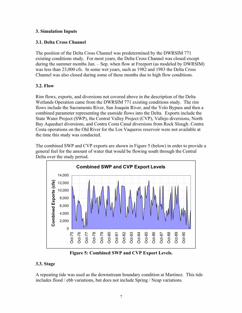
South Delta Permanent Gates The proposed future operation of the three South Delta agricultural permanent gates (Old River at Tracy, Middle River, and Grant Line Canal) and the fish protection barrier at Old River at Head was used in this study. When operating, the gates only allowed flow in the upstream direction. Each structure may be either installed or removed during the 13 planning periods, see Figure 3.1 below. Each month represents one planning period, with the exception of April, which is divided into two planning periods. This was done so the gates could be installed in the middle of the month, per the proposed future operation of the gates.

Barrier Oct Nov Dec Jan Feb Mar Apr May Jun Jul Aug Sep

Old River @ Head Old River @ Tracy

Middle River Grant Line Canal

Figure 3.1: Schedule of Permanent Barrier Operations.

Other Gates The Suisun Marsh Salinity Control Gate was operated October through May of each year. The Clifton Court Forebay Gates allowed water into the Forebay from the Old River when a difference in stage occurred between the river and the Forebay. This was referred to as a priority four operation in previous DSM2 planning studies.11 Water was not allowed to leave the Forebay.

3.2 Quality Water quality inputs were applied both at the external boundaries and at the Delta interior locations through use of the Delta Island Consumptive Use (DICU) model. Furthermore, QUAL was modified to account for increases in DOC stored in the project reservoirs based on research conducted by Jung (2001a). The sources and nature of these data are discussed below.

10 The SWRCB D-1641 standards for the DCC stipulate that the DCC must be closed when: (1) flow in the

Sacramento River is greater than 23,000 cfs, (2) for 45 days in Nov. - Jan., and (3) Feb. - May. 11 There are four different typical schedules of operation of the Clifton Court Forebay Gates that were used in

previous DSM2 planning studies. These schedules were designed to optimize the amount of water entering the Forebay, while minimizing the impact on South Delta stage. The work to create these different priority operations in DSM2 with the new historical-based tide used at Martinez is not yet completed.

-10-

3.2.1 EC As discussed above in Section 2.1, Martinez EC was generated using Net Delta Outflow (calculated from the CALSIM II results) and an updated G-model, based on work done by Ateljevich (2001a). CALSIM II provided monthly EC values for the San Joaquin River. Using the daily San Joaquin River flow and the monthly EC values, daily EC values were derived. The EC concentration at the remaining tributary boundaries, the Sacramento River, the Yolo Bypass, and the eastside streams, was fixed at 200 umhos/cm. Standard DICU data developed from the DICU model were used to represent the quality of water draining off the Delta islands. For the base case all of the standard DICU node locations and EC concentrations were used. For the alternative case the standard DICU node EC concentrations were used, but as discussed above in Section 2.2.4, the diversions and return flows were altered.

3.2.2 DOC Jung (2001a) reports that flooding Delta islands may result in increases in the DOC, due in part to peat soil DOC releases. A series of experiments were conducted to find the rate of DOC growth on Delta islands, and then a conceptual model was created to simulate this DOC growth. QUAL was modified to account for increases in DOC due to storage, using Equation 1 (see Jung 2001a).

( )1 kt

ADOC tBe−=

+ [Eqn. 1]

where

A = maximum island DOC concentration (mg/l), B = initial DOC concentration of diversion into island, k = growth rate of DOC (days-1), and t = time relative to initial diversion into island (days). Two different bookend simulations were run, to represent low and high ranges of DOC released from the islands. A summary of the coefficients used in Equation 1 and the range of DOC releases as modeled in QUAL is shown in Table 3.1. The initial DOC concentration was calculated within QUAL and takes the depth of the reservoir into account. This term is hardwired into QUAL. For most of the releases the DOC coming off the islands was less than the maximum values listed below.

Table 3.1: QUAL DOC Bookends. Bookend A

(mg/l) k

(days-1) Range of Released

DOC Low 70 0.022 6 - 10 mg/l High 215 0.022 13 - 22 mg/l

-11-

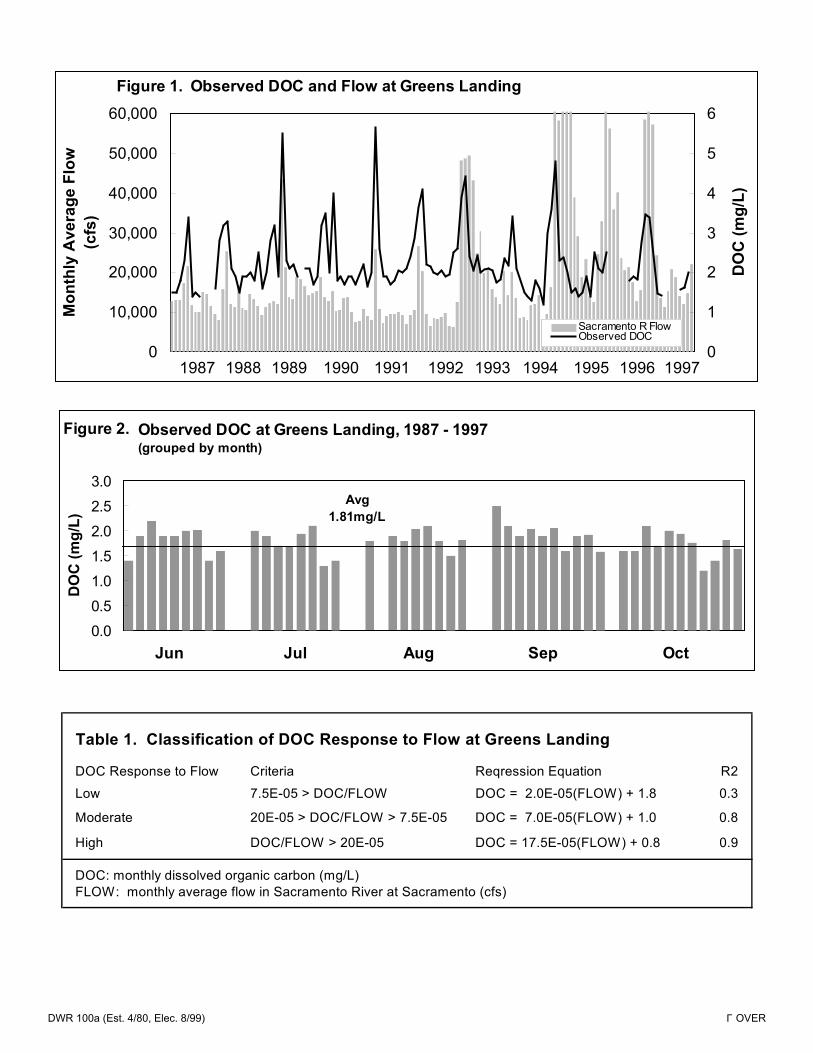
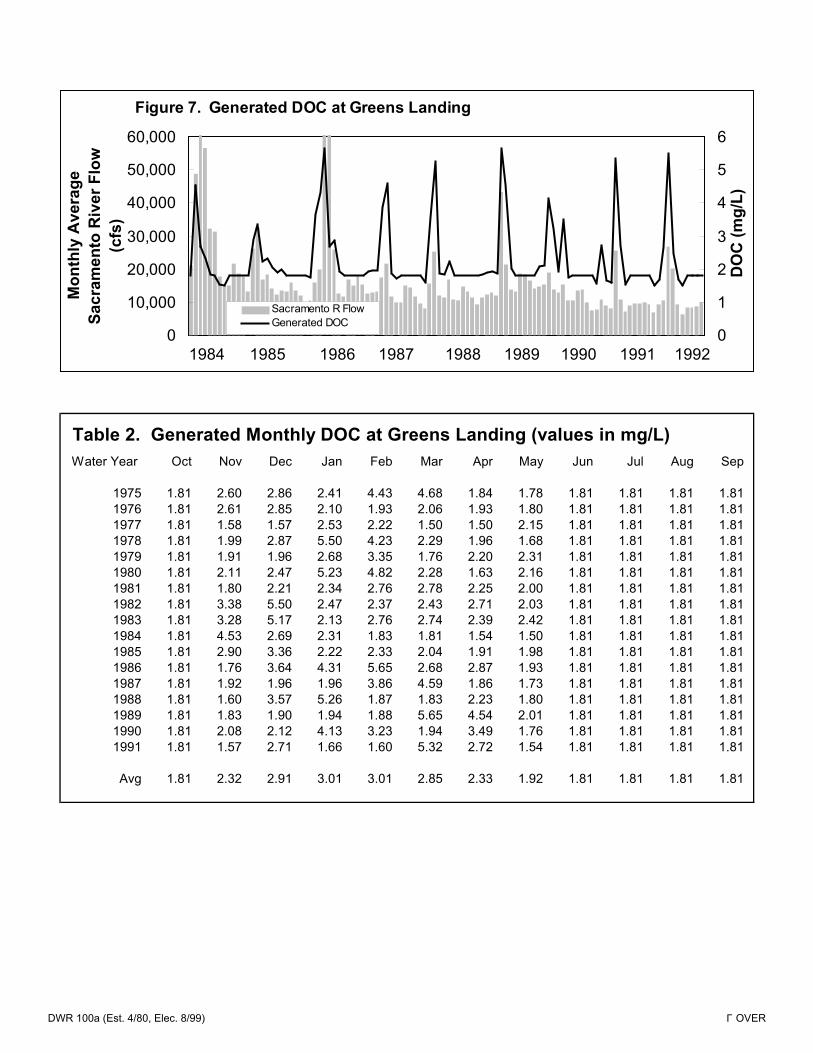
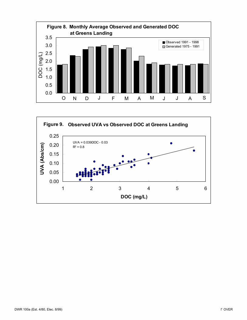
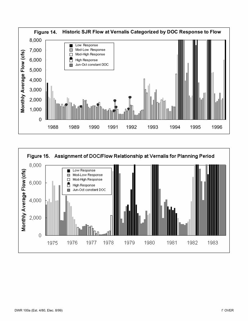
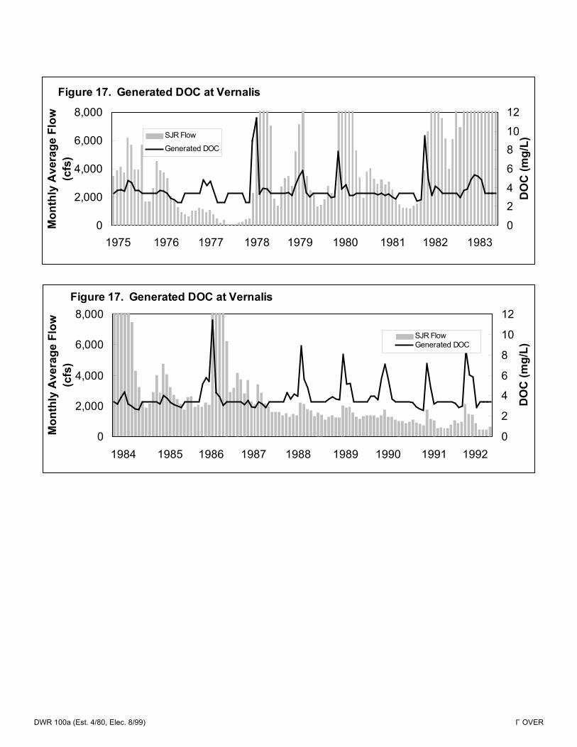
Another area that would affect DOC growth in the project islands is bioproductivity. This was not considered in these simulations. The DOC concentrations for the San Joaquin River, Sacramento River, and eastside streams were developed based on MWQI observations taken from 1987 through 1998 (Suits, 2001a). The summer DOC concentrations were based on monthly averages of the June through October observations. The winter DOC concentrations were generated using relationships relating DOC to flow. These relations were then used to create DOC concentrations for the three tributary boundary locations for the entire 16-year simulation period. The Sacramento River DOC concentrations were also applied to the Yolo Bypass flows. The range of the DOC concentrations at the rim boundaries is summarized in Table 3.2 below.

Table 3.2: Range of Tributary Boundary DOC (mg/l) Concentrations. San Joaquin Sacramento Eastside Streams DOC Range 2.40 - 11.40 1.81 - 5.65 1.66 - 3.95

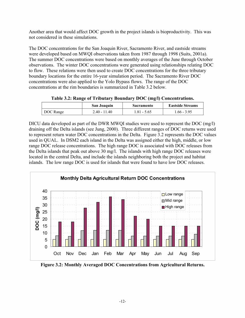
DICU data developed as part of the DWR MWQI studies were used to represent the DOC (mg/l) draining off the Delta islands (see Jung, 2000). Three different ranges of DOC returns were used to represent return water DOC concentrations in the Delta. Figure 3.2 represents the DOC values used in QUAL. In DSM2 each island in the Delta was assigned either the high, middle, or low range DOC release concentrations. The high range DOC is associated with DOC releases from the Delta islands that peak out above 30 mg/l. The islands with high range DOC releases were located in the central Delta, and include the islands neighboring both the project and habitat islands. The low range DOC is used for islands that were found to have low DOC releases.

Monthly Delta Agricultural Return DOC Concentrations

05

10152025303540


DO

C (m

g/l)

Low rangeMid rangeHigh range

Figure 3.2: Monthly Averaged DOC Concentrations from Agricultural Returns.

-12-

3.3 Initial Conditions DSM2 planning studies cover a 16-year period from Oct. 1975 to Sep. 1991. Unlike HYDRO, QUAL requires a much longer start-up period. In the case of planning studies, no assumption is made about the initial water quality conditions in the Delta; thus an extra year is run in order to simulate the mixing of the Delta. This is called a cold start routine. Both HYDRO and QUAL are run for this extra year, but the results are disregarded during this cold start period.

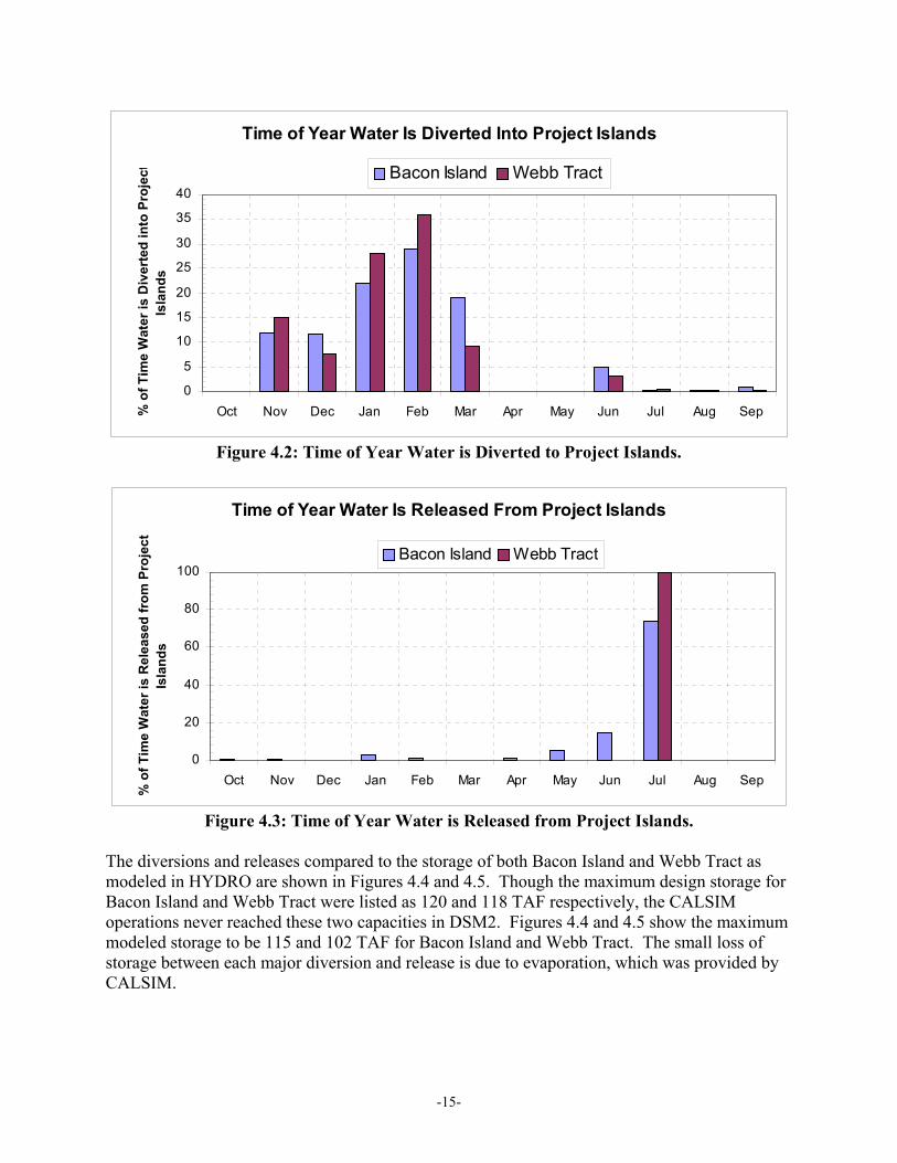
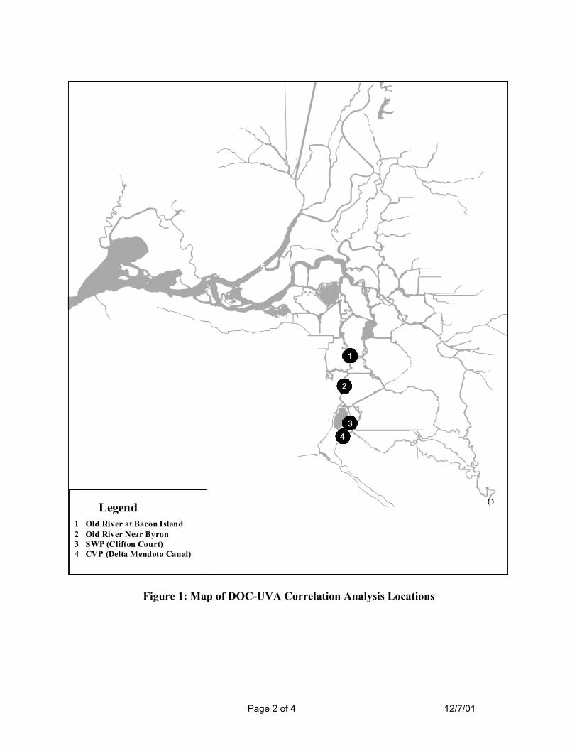
4 Results This report discusses five water quality constituents, chloride, dissolved organic carbon (DOC), ultraviolet absorbance at 254 nm (UVA), total trihalomethane (TTHM), and bromate. The long-term impacts on chloride and DOC are also discussed. QUAL was used to simulate EC and DOC, and then these constituents were used to calculate chloride, UVA, TTHM and bromate formation potentials. Modeled water quality at the following locations are shown below in Figure 4.1 for the entire planning period (1975 - 1991): Contra Costa's Rock Slough intake near the Old River, Contra Costa's Los Vaqueros intake on the Old River, the SWP and CVP intakes at Banks and Tracy Pumping Plants. These DSM2 output locations correspond with field sampling locations. This report focuses only on water quality at these locations. For the alternative simulation, the percentage of the time of year water was diverted to and later released from the project islands for the entire study period is shown in Figures 4.2 and 4.3. Generally the islands were filled in the winter months (Nov., Dec., Jan., Feb. and Mar.) and emptied in the summer months (Jun. and Jul.). Webb Tract is filled and emptied after Bacon Island has reached capacity; hence 100% of its releases are in July. During the summer months, CALSIM II frequently diverted small amounts of water to the project islands to account for evaporation losses.

-13-

Figure 4.1: Location of In-Delta Storage Project Islands and DSM2 Output Locations.

-14-

Time of Year Water Is Diverted Into Project Islands

0

5

10

15

20

25

30

35

40

Oct Nov Dec Jan Feb Mar Apr May Jun Jul Aug Sep% o

f Tim

e W

ater

is D

iver

ted

into

Pro

ject

Isla

nds

Bacon Island Webb Tract

Figure 4.2: Time of Year Water is Diverted to Project Islands.

Time of Year Water Is Released From Project Islands

0

20

40

60

80

100


% o

f Tim

e W

ater

is R

elea

sed

from

Pro

ject

Is

land

s


Figure 4.3: Time of Year Water is Released from Project Islands.

The diversions and releases compared to the storage of both Bacon Island and Webb Tract as modeled in HYDRO are shown in Figures 4.4 and 4.5. Though the maximum design storage for Bacon Island and Webb Tract were listed as 120 and 118 TAF respectively, the CALSIM operations never reached these two capacities in DSM2. Figures 4.4 and 4.5 show the maximum modeled storage to be 115 and 102 TAF for Bacon Island and Webb Tract. The small loss of storage between each major diversion and release is due to evaporation, which was provided by CALSIM.

-15-

Bacon Island Storage with Diversions and Releases

0

250

500

750

1000

1250

1500

1750

2000

Oct-75 Oct-76 Oct-77 Oct-78 Oct-79 Oct-80 Oct-81 Oct-82 Oct-83

Mon

thly

Ave

rage

d Fl

ow

(cfs

)

0

25

50

75

100

125

150

175

200

Stor

age

(TA

F)

Release Diversion Storage

Figure 4.4a: Bacon Island Storage with Diversions and Releases 1975 - 1983.

Bacon Island Storage with Diversions and Releases

0

250

500

750

1000

1250

1500

1750

2000

Oct-83 Oct-84 Oct-85 Oct-86 Oct-87 Oct-88 Oct-89 Oct-90

Mon

thly

Ave

rage

d Fl

ow (c

fs)

0

25

50

75

100

125

150

175

200

Stor

age

(TA

F)


Figure 4.4b: Bacon Island Storage with Diversions and Releases 1983 - 1991.

-16-

Webb Tract Storage with Diversions and Releases

0

250

500

750

1000

1250

1500

1750

2000


Mon

thly

Ave

rage

d Fl

ow

(cfs

)

0

25

50

75

100

125

150

175

200

Stor

age

(TA

F)


Figure 4.5a: Webb Tract Storage with Diversions and Releases 1975 - 1983.

Webb Tract Storage with Diversions and Releases

0

250

500

750

1000

1250

1500

1750

2000


Mon

thly

Ave

rage

d Fl

ow (c

fs)

0

25

50

75

100

125

150

175

200

Stor

age

(TA

F)


Figure 4.5b: Webb Tract Storage with Diversions and Releases 1983 - 1991.

-17-

4.1 Chloride As described above in Table 2.2.1 (see Section 2.2), two reservoirs were created in DSM2 to simulate chloride (modeled as EC in QUAL) coming from the two project islands: Bacon Island and Webb Tract. These reservoirs were connected to the Delta in DSM2 by using object-to-object transfers. This technique controlled when water would be added to or removed from the reservoirs. Since the chloride concentration of the reservoir islands is a function of the chloride around the intakes and the current chloride concentration in each island reservoir, QUAL was able to store the water and account for changes in water quality due to mixing, as shown in Equation 2 where concentrations are represented by C and volumes are represented by V. The only time chloride concentration in the islands would change was when water was diverted into the islands, which can be seen in Figures 4.6 and 4.7.

islandlows

islandislandlowslowsnew VV

VCVCC

++

=inf

infinf [Eqn. 2]

If the EC concentration of the water at the intakes were lower than the EC levels inside the island reservoir, then the inflows would reduce the island EC concentration. If the EC concentration of the water at the intakes were higher than the EC levels inside the island, then the inflows would increase the island EC concentration. Discharges from the islands did not change the water quality of the reservoirs and had little impact on the EC concentration in the Delta itself.

Changes in Bacon Island EC due to Bacon Island Diversions and Releases

0500

1000150020002500


Mon

thly

Ave

rage

d Fl

ow (c

fs)

0100200300400500

EC (u

mho

s/cm

)

Releases Diversions Bacon Island EC

Figure 4.6a: Changes in Bacon Island EC due to Project Diversions and Releases 1976-1983.

Changes in Bacon Island EC due to Bacon Island Diversions and Releases

0500

1000150020002500


Mon

thly

Ave

rage

d Fl

ow (c

fs)

0100200300400500

EC (u

mho

s/cm

)

Releases Diversions Bacon Island EC

Figure 4.6b: Changes in Bacon Island EC due to Project Diversions and Releases 1983-1991.

-18-

Changes in Webb Tract EC due to Webb Tract Diversions and Releases

0

500

1000

1500

2000


Mon

thly

Ave

rage

d Fl

ow (c

fs)

050100150200250300

EC (u

mho

s/cm

)

Releases Diversions Webb Tract EC

Figure 4.7a: Changes in Webb Tract EC due to Project Diversions and Releases 1976-1983.

Changes in Webb Tract EC due to Webb Tract Diversions and Releases

0

500

1000

1500

2000


Mon

thly

Ave

rage

d Fl

ow (c

fs)

050100150200250300

EC (u

mho

s/cm

)

Releases Diversions Webb Tract EC

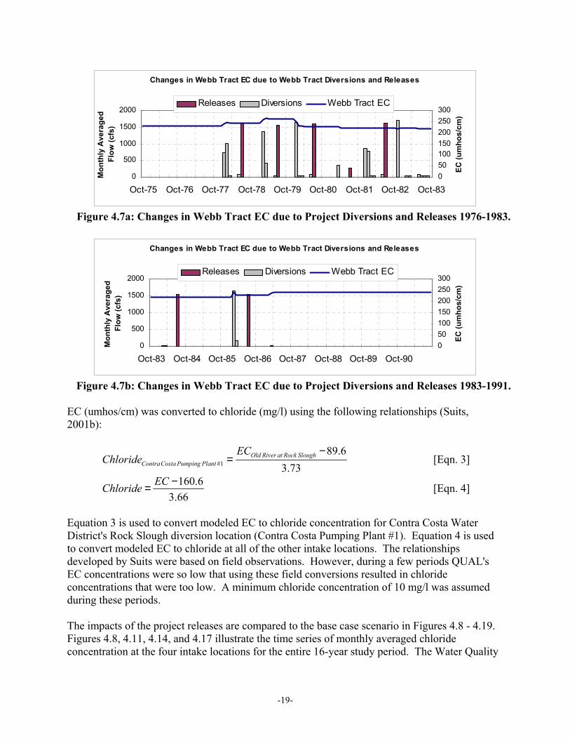
Figure 4.7b: Changes in Webb Tract EC due to Project Diversions and Releases 1983-1991.

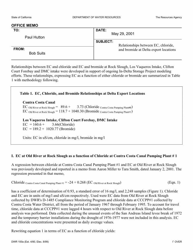
EC (umhos/cm) was converted to chloride (mg/l) using the following relationships (Suits, 2001b):

#1

89.63.73

Old River at Rock SloughContraCosta Pumping Plant

ECChloride

−= [Eqn. 3]

160.63.66

ECChloride −= [Eqn. 4]

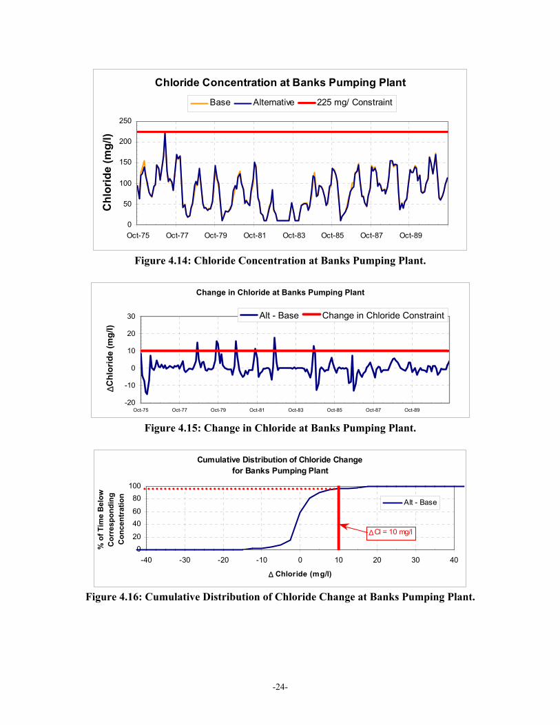
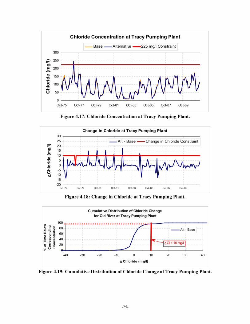
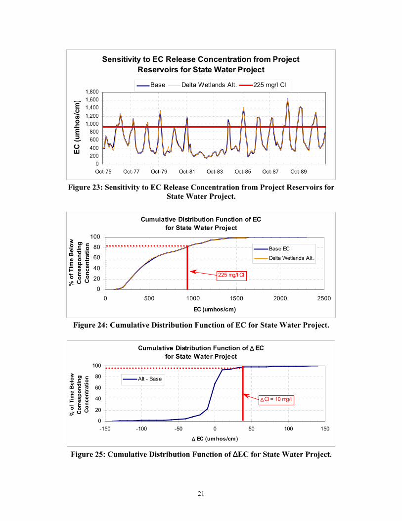
Equation 3 is used to convert modeled EC to chloride concentration for Contra Costa Water District's Rock Slough diversion location (Contra Costa Pumping Plant #1). Equation 4 is used to convert modeled EC to chloride at all of the other intake locations. The relationships developed by Suits were based on field observations. However, during a few periods QUAL's EC concentrations were so low that using these field conversions resulted in chloride concentrations that were too low. A minimum chloride concentration of 10 mg/l was assumed during these periods. The impacts of the project releases are compared to the base case scenario in Figures 4.8 - 4.19. Figures 4.8, 4.11, 4.14, and 4.17 illustrate the time series of monthly averaged chloride concentration at the four intake locations for the entire 16-year study period. The Water Quality

-19-

Management Plan (WQMP, 2000) 225 mg/l chloride constraint is shown on these figures. The WQMP limited this constraint to be 90% of existing D-1641 salinity standards (Hutton, 2001). The 225 mg/l WQMP chloride constraint was exceeded at the Old River at Rock Slough and Tracy (CVP) intake locations for both the base and alternative studies in 1977. The WQMP constraint was not exceeded in either scenario at the Los Vaqueros or Banks (SWP) intake locations. The maximum monthly averaged chloride for the four intake locations is listed in Table 4.1. All of these maximums occurred in 1977. The maximum monthly averaged chloride concentration was larger in the alternative than in the base study at all four locations.

Table 4.1: Maximum Monthly Averaged Cl (mg/l). Location Base Alternative Old River at Rock Slough 235 243 Old River at Los Vaqueros Intake 191 197 Banks Pumping Plant (SWP) 222 223 Tracy Pumping Plant (CVP) 246 247

The WQMP stipulated that the maximum increase in chloride concentration due to operation of the project is 10 mg/l when the base case chloride concentration is less than the 225 mg/l constraint, otherwise no increase is allowed (Hutton, 2001). Time series of the difference between the alternative and base case chloride results for the four intake locations and change in chloride concentration constraint for the 16-year period are illustrated in Figures 4.9, 4.12, 4.15, and 4.18. The maximum increase in monthly averaged chloride when this incremental 10 mg/l constraint applies is listed in Table 4.2. The WQMP incremental chloride constraint is exceeded at all four urban intake locations during the 16-year simulation.

Table 4.2: Maximum Increase in Monthly Averaged Cl (mg/l)

When Base Chloride is Less Than 225 mg/l. Location Alt. - Base Old River at Rock Slough 32 Old River at Los Vaqueros Intake 25 Banks Pumping Plant (SWP) 18 Tracy Pumping Plant (CVP) 18

The Cumulative Distribution Function (cdf) for the change (measured as alternative - base case) in chloride concentration at each location is shown in Figures 4.10, 4.13, 4.16, and 4.19. These cdfs were calculated based on a frequency histogram of the difference in chloride concentration (alternative - base) for every month of the entire 16-year simulation. Each cdf curve represents the amount of time that the chloride concentration is equal to or less than a corresponding chloride level. These figures illustrate that over the study period that the overall changes in chloride tended to be between -20 and 20 mg/l. These plots are useful in measuring the impact of the In-Delta Storage project operations on the four urban intake locations. A summary of the percent of time that this increase in salinity (alternative - base) exceeded the WQMP constraint is shown below in Table 4.3. The largest increase in chloride was at Old

-20-

River at Rock Slough, where the WQMP chloride constraint was exceeded approximately 5.7% of the time.

Table 4.3: Percent of time that the change in Cl is larger than 10 mg/l. Location % Exceedance Old River at Rock Slough 5.7 Old River at Los Vaqueros Intake 5.2 Banks Pumping Plant (SWP) 3.6 Tracy Pumping Plant (CVP) 3.6

The number of months that the two WQMP Cl constraints were exceeded for both the base and alternative simulations is shown below in Table 4.4. The values in Table 4.4 were taken from the entire 16-year (192 month) period, however the project only diverted or released water during 75 of these months.12 The last column in Table 4.4 shows the total number of months the WQMP Cl constraints were violated. If the 225 mg/l constraint was violated in the alternative, but not in the base case during a month that when the 10 mg/l change in Cl constraint was also exceeded, that month was not double counted.

Table 4.4: Number of Months of Exceedance of the WQMP Cl Standards.

225 mg/l Cl Constraint

10 mg/l Change in Cl Constraint

Total Number of Months in

Violation Location Base Alt Alt - Base Alt - Base Old River at Rock Slough 3 3 11 11 Old River at Los Vaqueros Intake 0 0 10 10 Banks Pumping Plant (SWP) 0 0 7 7 Tracy Pumping Plant (CVP) 1 1 7 7

The number of months in which the 225 mg/l Cl standard was violated was the same in both the base and alternative simulations. The largest number of total WQMP violations was at Rock Slough.

12 Out of the 192 months simulated, water was diverted into or released from the project islands during 75 months.

These diversions include the smaller flows that were taken by the project in order to account for evaporation losses. Many of these smaller diversions were less than 25 cfs, which is significantly smaller than many of the Delta island consumptive use diversions and return flows.

-21-

Chloride Concentration at Old River at Rock Slough

0

50

100

150

200

250

300


Chl

orid

e (m

g/l)

Base Alternative 225 mg/l Constraint

Figure 4.8: Chloride Concentration at Old River at Rock Slough.

Change in Chloride at Old River at Rock Slough

-40-30-20-10

01020304050


∆C

hlor

ide

(mg/

l)

Alt - Base Change in Cl Constraint

Figure 4.9: Change in Chloride at Old River at Rock Slough.

Cumulative Distribution of Chloride Change for Old River at Rock Slough

020406080

100

-40 -30 -20 -10 0 10 20 30 40

∆ Chloride (mg/l)

% o

f Tim

e B

elow

C

orre

spon

ding

C

once

ntra

tion

Alt - Base

∆Cl = 10 mg/l

Figure 4.10: Cumulative Distribution of Chloride Change at Old River at Rock Slough.

-22-

Chloride Concentration at Old River at Los Vaqueros Intake

0

50

100

150

200

250


Chl

orid

e (m

g/l)


Figure 4.11: Chloride Concentration at Old River at Los Vaqueros Intake.

Change in Chloride at Old River at Los Vaqueros Intake

-30-20-10

01020304050


∆C

hlor

ide

(mg/

l)

Alt - Base Change in Chloride Constraint

Figure 4.12: Change in Chloride at Old River at Los Vaqueros Intake.

Cumulative Distribution of Chloride Change for Old River at Los Vaqueros Intake

0

2040

6080

100

-40 -30 -20 -10 0 10 20 30 40

∆ Chloride (mg/l)

% o

f Tim

e B

elow

C

orre

spon

ding

C

once

ntra

tion

Alt - Base

∆Cl = 10 mg/l

Figure 4.13: Cumulative Distribution of Chloride Change at Old River at Los Vaqueros Intake.

-23-

Chloride Concentration at Banks Pumping Plant

0

50

100

150

200

250


Chl

orid

e (m

g/l)

Base Alternative 225 mg/ Constraint

Figure 4.14: Chloride Concentration at Banks Pumping Plant.

Change in Chloride at Banks Pumping Plant

-20

-10

0

10

20

30


∆C

hlor

ide

(mg/

l)


Figure 4.15: Change in Chloride at Banks Pumping Plant.

Cumulative Distribution of Chloride Change for Banks Pumping Plant

020

4060

80100

-40 -30 -20 -10 0 10 20 30 40

∆ Chloride (mg/l)

% o

f Tim

e B

elow

C

orre

spon

ding

C

once

ntra

tion

Alt - Base

∆Cl = 10 mg/l

Figure 4.16: Cumulative Distribution of Chloride Change at Banks Pumping Plant.

-24-

Chloride Concentration at Tracy Pumping Plant

0

50

100

150

200

250

300


Chl

orid

e (m

g/l)


Figure 4.17: Chloride Concentration at Tracy Pumping Plant.

Change in Chloride at Tracy Pumping Plant

-20-15-10-505

1015202530


∆C

hlor

ide

(mg/

l)


Figure 4.18: Change in Chloride at Tracy Pumping Plant.

Cumulative Distribution of Chloride Change for Old River at Tracy Pumping Plant

020406080

100

-40 -30 -20 -10 0 10 20 30 40

∆ Chloride (mg/l)

% o

f Tim

e B

elow

C

orre

spon

ding

C

once

ntra

tion

Alt - Base

∆Cl = 10 mg/l

Figure 4.19: Cumulative Distribution of Chloride Change at Tracy Pumping Plant.

-25-

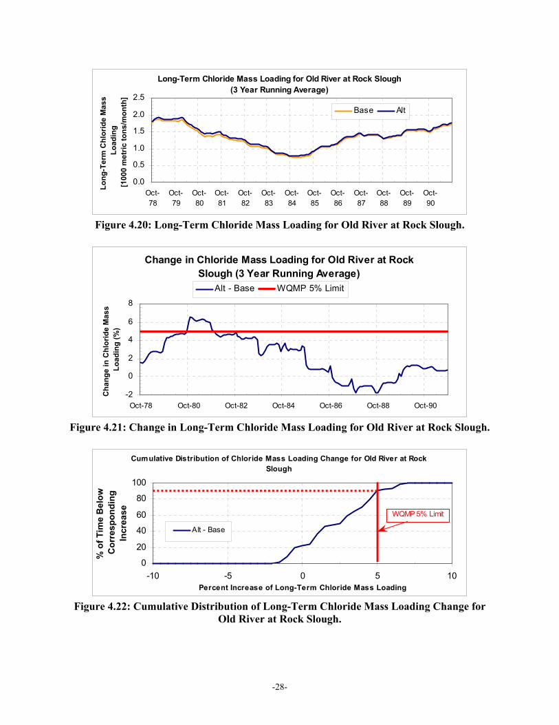
4.2 Long-Term Chloride Long-term increases due to the operation of the project were calculated as the 3-year running average of monthly average chloride mass loading (see Hutton, 2001). Time series plots of the long-term monthly averaged chloride mass loading (expressed in 1000 metric tons / month) at Old River at Rock Slough and the State Water Project and the Central Valley Project intakes are shown in Figures 4.20, 4.23, and 4.26.13 The long-term impact of the project operations was calculated using Equation 5.

/ //

/

% 100%w Project w o projectIncreasew Project

w o project

Chloride ChlorideChloride

Chloride−

= × [Eqn. 5]

The WQMP limits the long-term chloride mass loading increases at the intake locations due to the project operation to 5%. This 5% limit is shown on the time series plots (Figures 4.21, 4.24, and 4.27) of the long-term percent increase of chloride mass loading. The maximum percent increase in the long-term monthly averaged chloride mass loading is shown in Table 4.5. The alternative simulation exceeded the WQMP 5% increase constraint at Old River at Rock Slough and the Banks Pumping Plant, but the operation of the project only met the 5% increase constraint at the Tracy Pumping Plant.

Table 4.5: Maximum Percent Increase in Long-Term Monthly Averaged Chloride Mass Loading.

Location Percent Increase Old River at Rock Slough 6.6 Banks Pumping Plant (SWP) 6.5 Tracy Pumping Plant (CVP) 5.0

Frequency histograms of the percent increase in long-term chloride mass loading for the entire simulation period were used to create cumulative distribution functions (cdfs) to represent the long-term impact of the project operations. These cdfs are shown in Figures 4.22, 4.25, and 4.28. The WQMP maximum 5% increase in long-term chloride mass loading constraint is shown on each figure. The percent of the time that each scenario was equal to or below the WQMP maximum 5% increase constraint is listed in Table 4.6.

13 Normally Contra Costa Water District (CCWD) diversions are divided between the Rock Slough and Los

Vaqueros Reservoir intakes. Long-term chloride mass loading was not calculated for Old River at Los Vaqueros Reservoir intake because CALSIM II did not separate the CCWD diversions. Similarly, the mass loading calculated for Rock Slough is based on the assumption that 100% of CCWD's diversions would be taken at the Rock Slough location.

-26-

Table 4.6: Percent Time that the Percent Increase of Long-Term Chloride Mass Loading Exceeds the WQMP Maximum 5% Increase Constraint.

Location % Exceedance Old River at Rock Slough 9 Banks Pumping Plant (SWP) 5 Tracy Pumping Plant (CVP) 0

The number of months out of the 156 months that the long-term chloride mass loading increase exceeds the WQMP 5% increase constraint is shown below in Table 4.7.14 Old River at Rock Slough experienced the largest number of violations (14 months) of the constraint.

Table 4.7: Number of Months the Long-Term Chloride Mass Loading

Increase Exceeds the WQMP 5% Increase Constraint. Location 5% Increase Constraint Old River at Rock Slough 14 Banks Pumping Plant (SWP) 8 Tracy Pumping Plant (CVP) 0

14 Instead of 192 months, the long-term mass loading calculations used the first 36 months to calculate the running

average, thus long-term violations come from a sample of only 156 months.

-27-

Long-Term Chloride Mass Loading for Old River at Rock Slough(3 Year Running Average)

0.0

0.5

1.0

1.5

2.0

2.5

Oct-78

Oct-79

Oct-80

Oct-81

Oct-82

Oct-83

Oct-84

Oct-85

Oct-86

Oct-87

Oct-88

Oct-89

Oct-90

Long

-Ter

m C

hlor

ide

Mas

s Lo

adin

g[1

000

met

ric to

ns/m

onth

]Base Alt

Figure 4.20: Long-Term Chloride Mass Loading for Old River at Rock Slough.

Change in Chloride Mass Loading for Old River at Rock Slough (3 Year Running Average)

-2

0

2

4

6

8

Oct-78 Oct-80 Oct-82 Oct-84 Oct-86 Oct-88 Oct-90

Cha

nge

in C

hlor

ide

Mas

s Lo

adin

g (%

)

Alt - Base WQMP 5% Limit

Figure 4.21: Change in Long-Term Chloride Mass Loading for Old River at Rock Slough.

Cumulative Distribution of Chloride Mass Loading Change for Old River at Rock

Slough

0

20

40

60

80

100

-10 -5 0 5 10Percent Increase of Long-Term Chloride Mass Loading

% o

f Tim

e B

elow

C

orre

spon

ding

In

crea

se

Alt - Base

WQMP 5% Limit

Figure 4.22: Cumulative Distribution of Long-Term Chloride Mass Loading Change for Old River at Rock Slough.

-28-

Long-Term Chloride Mass Loading at Banks Pumping Plant(3 Year Running Average)

05

1015

2025

30

Oct-78

Oct-79

Oct-80

Oct-81

Oct-82

Oct-83

Oct-84

Oct-85

Oct-86

Oct-87

Oct-88

Oct-89

Oct-90

Long

-Ter

m C

hlor

ide

Mas

sLo

adin

g[1

000

met

ric to

ns/m

onth

]

Base Alt.

Figure 4.23: Long-Term Chloride Mass Loading for Banks Pumping Plant.

Change in Chloride Mass Loading at Banks Pumping Plant(3 Year Running Average)

-4

-2

0

2

4

6

8


Cha

nge

in C

hlor

ide

Mas

sLo

adin

g (%

)


Figure 4.24: Change in Long-Term Chloride Mass Loading for Banks Pumping Plant.

Cumulative Distribution of Chloride Mass Loading Change at Banks Pumping

Plant

0

20

40

60

80

100

-10 -5 0 5 10Chloride Mass Loading Change (%)

% o

f Tim

e B

elow

C

orre

spon

ding

In

crea

se

Alt - Base

WQMP 5% Limit

Figure 4.25: Cumulative Distribution of Long-Term Chloride Mass Loading Change for Banks Pumping Plant.

-29-

Long-Term Chloride Mass Loading for Tracy Pumping Plant(3 Year Running Average)

0

5

10

15

20

25

Oct-78

Oct-79

Oct-80

Oct-81

Oct-82

Oct-83

Oct-84

Oct-85

Oct-86

Oct-87

Oct-88

Oct-89

Oct-90

Long

-Ter

m C

hlor

ide

Mas

s Lo

adin

g[1

000

met

ric to

ns/m

onth

]

Base Alt

Figure 4.26: Long-Term Chloride Mass Loading for Tracy Pumping Plant.

Change in Long-Term Chloride Mass Loading forTracy Pumping Plant (3 Year Running Average)

-3-2-10123456


Cha

nge

in C

hlor

ide

Mas

sLo

adin

g (%

)


Figure 4.27: Change in Long-Term Chloride Mass Loading for Tracy Pumping Plant.

Cumulative Distribution of Chloride Mass Loading Changes for Tracy Pumping

Plant

0

20

40

60

80

100

-10 -5 0 5 10Percent Increase of Long Term DOC Mass Loading

% o

f Tim

e B

elow

C

orre

spon

ding

In

crea

se

Alt - Base

WQMP 5% Limit

Figure 4.28: Cumulative Distribution of Long-Term Chloride Mass Loading Change for Tracy Pumping Plant.

-30-

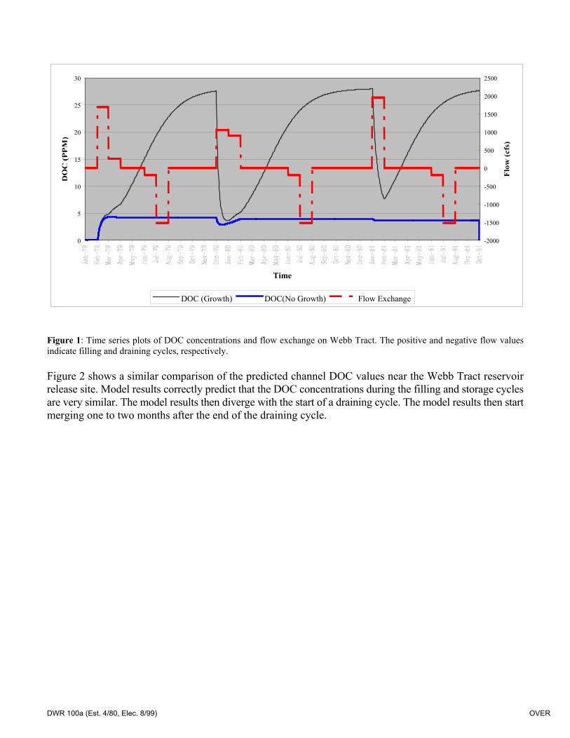
4.3 DOC As discussed in Section 3.2.2, QUAL was modified to simulate increases in DOC related to the use of the project islands as reservoirs. Two bookend values were chosen to represent realistic upper and lower bounds of reservoir based growth in DOC. The impact of these modifications on DOC in both Bacon Island and Webb Tract are shown in Figures 4.29 and 4.30. The maximum-modeled DOC in the project islands was 10 and 22 mg/l for the low and high bookend conditions respectively. When water was diverted into the reservoirs, the DOC in the reservoirs was recalculated using Equation 1 with new initial conditions (the current stage in the reservoir and the DOC concentration of the incoming diversion). The DOC in the reservoirs continued to grow at a rate specified by Equation 1 until the next diversion. This can be best seen in Figure 4.29a, where each drop in Bacon Island DOC corresponds with a diversion into the reservoir. In some cases the incoming DOC from neighboring channels was higher than the asymptotic (theoretical maximum) value for the low-bookend. The parameters used in Equation 1 could result in the DOC growth formulation effectively removing or lowering the DOC concentration in an island reservoir if the concentration of an incoming diversion was higher than the theoretical maximum. For example, it is shown in Figure 4.29a that the low-bookend DOC tends to flatten out around 6.3 mg/l. Based on the parameters chosen for the low-bookend (see Section 3.2.2) and the depth of Bacon Island during a typical diversion period, the maximum low-bookend should be around 6.3 mg/l. However, there are a few periods in which the low-bookend DOC shown in Figure 4.29a exceeds 8 mg/l. The incoming DOC at these times was greater than 6.3 mg/l. In the original post-processing (these results are not shown) of the DSM2 results, the low-bookend application of Equation 1 then slowly lowered the DOC concentration in Bacon Island until it once again reached the theoretical maximum of 6.3 mg/l. Instead of DOC growing, the DOC in Bacon Island appeared to decrease over time. Since the purpose of Jung’s DOC growth function was to account for increases in DOC concentration due to interactions between water and the peat soil of the island reservoirs, a third simulation where no DOC growth was accounted for was also run. In this third QUAL simulation, the DOC concentration in the island reservoirs would only be a function of the DOC concentration of incoming diversions and the DOC concentration already present in the island reservoirs. This simple mixing formulation is consistent with conservative water quality constituents, and was described by Equation 2 in Section 4.1. The time series of low-bookend DOC was then compared with the no growth DOC time series. For the few times that the no growth DOC time series was greater than the low-bookend DOC time series (and this would only happen when the implementation of Equation 1 resulted in reductions of island DOC concentrations), the no growth DOC time series data were used instead of the low-bookend data. The concentration of any release from either island can be found by simply looking at the reservoir concentration at the time of the release. It is important to note that the majority of the

-31-

releases did not occur when either island's DOC had yet reached its maximum values. The operations provided by CALSIM II resulted in carry-over storage in 1983 (i.e. water was stored in Bacon Island and Webb Tract for more than one year). The summer releases in 1984 from both islands were at the maximum DOC levels described above (NOTE: these 1984 releases did exceed the DOC standards, however, they do not represent the maximum violations of the WQMP standards, as will be described below).

Bacon Island DOC

0

500

1000

1500

2000


Mon

thly

Ave

rage

d Fl

ow

(cfs

)

0

5

10

15

20

DO

C (m

g/l)

Releases Diversions Low Bookend High Bookend

Figure 4.29a: Bacon Island DOC 1975 – 1983.

Bacon Island DOC

0

500

1000

1500

2000


Mon

thly

Ave

rage

d Fl

ow

(cfs

)

0

5

10

15

20

DO

C (m

g/l)


Figure 4.29b: Bacon Island DOC 1983 – 1991.

-32-

Webb Tract DOC

0

500

1000

1500

2000

2500


Mon

thly

Ave

rage

d Fl

ow

(cfs

)

0

5

10

15

20

25

DO

C (m

g/l)


Figure 4.30a: Webb Tract DOC 1975 – 1983.

Webb Tract DOC

0

500

1000

1500

2000

2500


Mon

thly

Ave

rage

d Fl

ow

(cfs

)

0

5

10

15

20

25

DO

C (m

g/l)


Figure 4.30b: Webb Tract DOC 1983 – 1991.

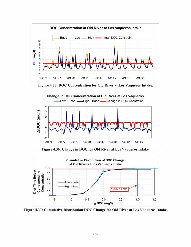
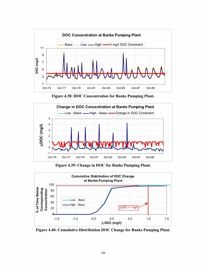
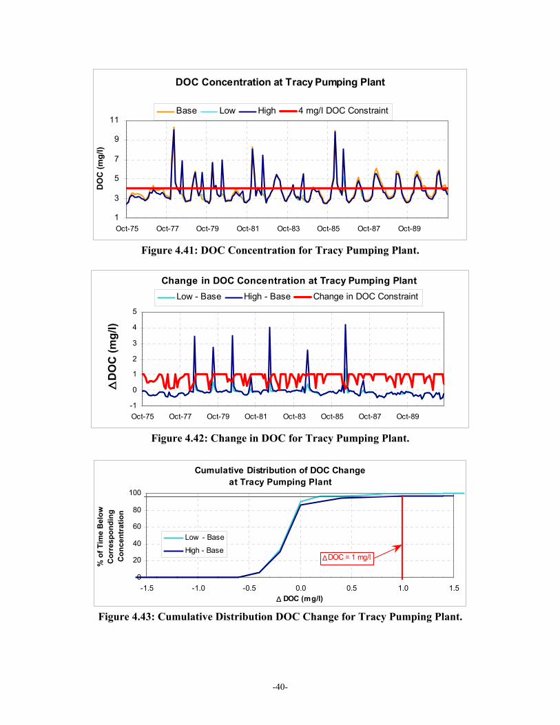
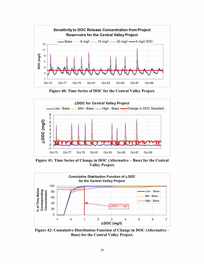
As discussed in Section 2.2, the consumptive use of both the project and habitat islands was modified to account for local changes in land use. These changes did not decrease the overall consumptive use in the Delta, but instead redirected water use from the project and habitat islands to other locations (see Section 2.2.4 for more details). Clearly these changes will have some impact on both hydrodynamics and water quality. However, the impact of similar changes to consumptive use on just the project islands was found to have a relatively small benefit (Mierzwa, 2001).15 Figures 4.32, 4.35, 4.38, and 4.41 illustrate the sensitivity to DOC release concentrations at each of the four urban intake locations: Old River at Rock Slough, Old River at the Los Vaqueros 15 It is recommended that future studies be conducted without operation of the project, but accounting for changes in

land use associated with the project. These studies could quantify the actual ag credit associated with changing the consumptive use of both the project and habitat islands.

-33-

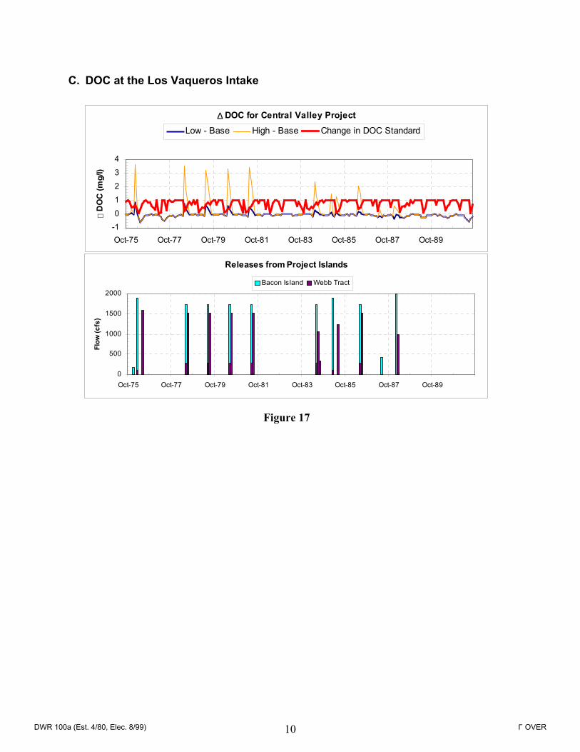
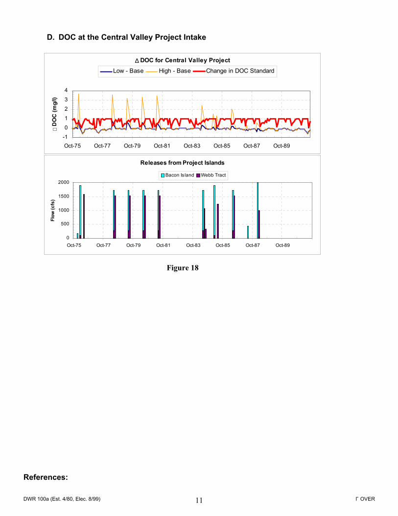
Intake, the State Water Project intake at Banks Pumping Plant, and the Central Valley Project intake at Tracy. A 4 mg/l DOC concentration is shown, which was later used to calculate the WQMP change in DOC constraint. The base case monthly averaged DOC concentration at Rock Slough ranged between 2.08 and 8.42 mg/l. Further south at the other three intake locations, the base case monthly averaged DOC concentrations increased slightly. The base case DOC frequently exceeded the 4 mg/l concentration level at all four locations. During the times when the base case DOC exceeded the 4 mg/l concentration level, both the low- and high-bookend simulations also exceeded 4 mg/l. However, releases from the project also resulted in additional times when the alternative simulations exceeded 4 mg/l. The maximum monthly averaged DOC at all four export locations over the entire 16-year planning study is summarized in Table 4.8.

Table 4.8: Maximum Monthly Averaged DOC (mg/l). Location Base Low Bookend High Bookend Old River at Rock Slough 8.42 7.73 7.73 Old River at Los Vaqueros Intake 8.81 8.19 8.19 Banks Pumping Plant (SWP) 10.01 9.50 9.50 Tracy Pumping Plant (CVP) 10.39 10.10 10.10

In all three simulations, the periods of maximum DOC for all of the locations coincided with the high runoff periods that start in the late winter and last through the spring. These periods of high DOC did not coincide with the major (summer) release periods associated with the operation of the project. Though summer project releases from the two alternative simulations did result in additional DOC spikes that approached the winter DOC maximums listed above, the concentration from the project releases did not exceed the maximums for either bookend. However, previous DSM2 studies have shown that other Delta Wetlands configurations can result in conditions where the summer project releases for both bookends can exceed the winter DOC concentrations (Mierzwa, 2001).

Table 4.9: Maximum Monthly Averaged Increase in DOC (mg/l). Location Low - Base High - Base Old River at Rock Slough 0.63 2.92 Old River at Los Vaqueros Intake 0.98 3.60 Banks Pumping Plant (SWP) 1.37 4.30 Tracy Pumping Plant (CVP) 1.36 4.21

As shown in Figures 4.29 and 4.30, the quality of the water released from the project islands typically ranged between 5 and 20 mg/l, which frequently is higher than the DOC concentration of the water already present in the channels around the project islands. The maximum monthly increase in DOC for each of the bookend scenarios is shown in Table 4.9. At all four intake locations, these increases were directly related to project releases. The largest increases occurred at the Banks Pumping Plant (SWP). Particle Tracking Model (PTM) simulations have shown that when high quantities of water is released from the island reservoirs, and the export capacity of Banks is increased to match this release, a large portion of this additional water ends up at the

-34-

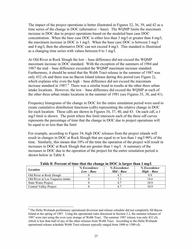
project pumps. This additional water typically has DOC concentrations equal to or higher than the concentration of the water coming from other sources, thus the largest increases in DOC concentrations were associated with the regions that also had the largest increases in exports. In other words, increased pumping at Banks would pull the water with higher DOC concentrations to both the Banks and Tracy Pumping Plants. The impact of the project operations is better illustrated in Figures 4.32, 4.35, 4.38, and 4.41 as a time series of the change in monthly averaged DOC (alternative - base). The WQMP limits the maximum increase in DOC due to project operations based on the modeled base case DOC concentration. When the base case DOC is either less than 3 mg/l or greater than 4 mg/l, the maximum increase in DOC is 1 mg/l. When the base case DOC is between 3 mg/l and 4 mg/l, then the alternative DOC can not exceed 4 mg/l (in other words, the maximum allowed increase is the difference between 4 mg/l and the base case). This constraint is shown below in Figure 4.31 and is illustrated in Figures 4.33, 4.36, 4.39, and 4.42 as a changing DOC constraint time series with values between 0 to 1 mg/l.

WQMP Incremental DOC Constraint

0.0

0.2

0.4

0.6

0.8

1.0

1.2

0 1 2 3 4 5

Modeled Base Case DOC (mg/l)

Max

imum

Allo

wed

DO

C (m

g/l)

Figure 4.31: WQMP Incremental DOC Constraint.

Both the low- and high-bookend simulations exceeded the WQMP's incremental increase constraint. The low-bookend simulation exceeded the incremental constraint at Banks and Tracy for 4 of the 8 major release periods. 16 The high-bookend simulation exceeded the incremental constraint at all four intake locations for 6 of the 8 major project releases during the 16-year simulation.17 Typical summer releases were made in July and averaged above 3000 cfs for the

16 Though during the entire 16-year (192 month) simulation water was released from the project island reservoirs 25

months, the combined flow released from the two project islands exceeded 500 cfs only 9 months or 8 different years (1978, 1979, 1980, 1981, 1982, 1984, 1986, and 1987). In 1979, 1981, 1984 and 1987 water was released in both June and July. June 1984 was the only time when a June release was larger than 500 cfs. These 8 different years are referred to as the major project releases or release periods.

17 The State Water Project and Central Valley Project exceeded the WQMP constraint for the high-bookend simulation for two months in the same release period (June and July in 1984), bringing the total number of months of violation to 7 for each location.

-35-

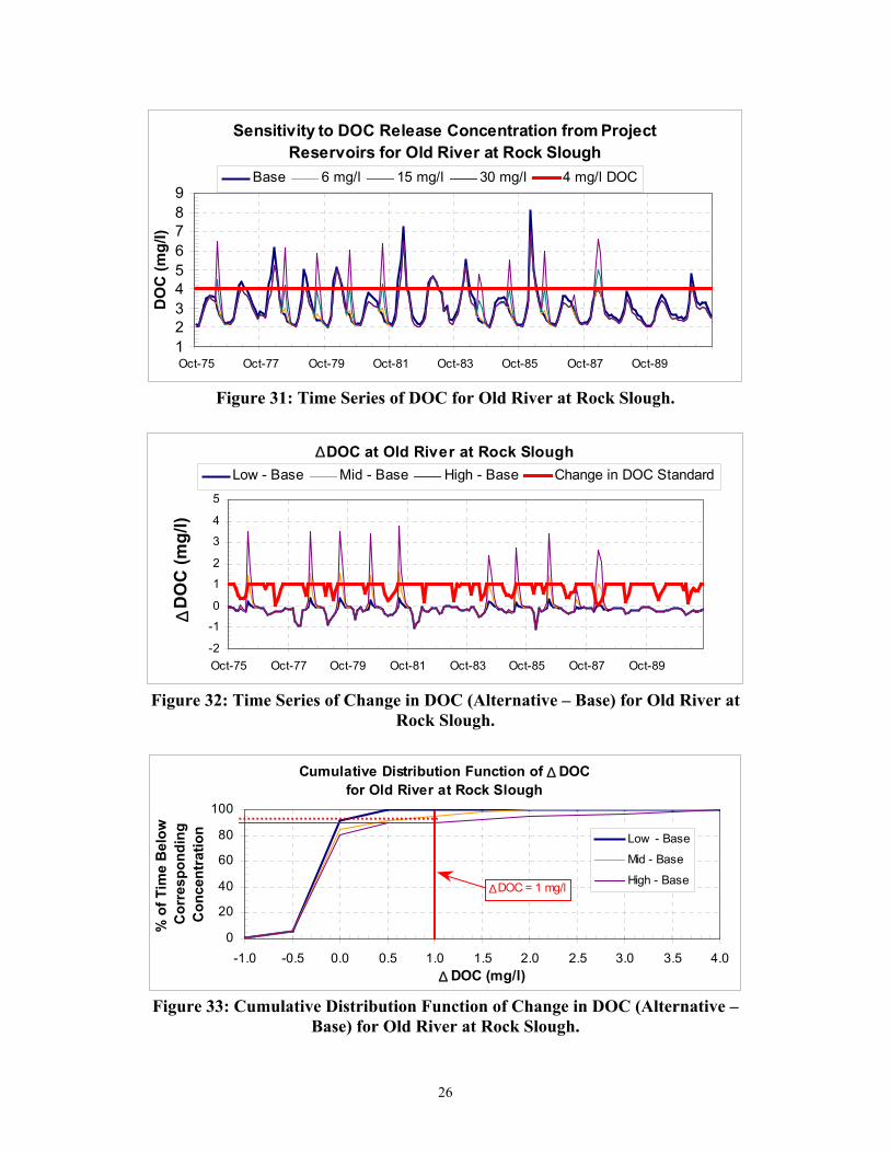
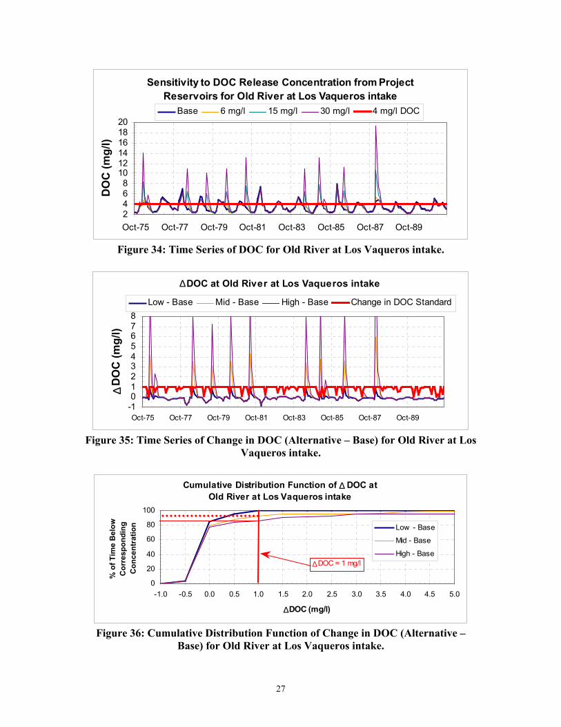
month. The project releases were less than 1500 cfs, during the two release periods (1981 and 1987) that did not exceed the constraint in the high-bookend simulation. Frequency histograms of the change in DOC for the entire simulation period were used to create cumulative distribution functions (cdfs) representing the relative change in DOC for each location. These cdfs are shown in Figures 4.34, 4.37, 4.40, and 4.43. On each cdf, a 1 mg/l limit is shown. The point where this limit intersects either of the curves represents the percentage of time that the change in DOC due to the project operations will be equal to or less than the WQMP limit. For example, according to Figure 4.34, high DOC releases from the project islands will result in changes in DOC at Rock Slough that is equal to or less than 1 mg/l approximately 97% of the time. Similarly, this means that approximately 3% of the time the operation of the project will result in increases in DOC at Rock Slough that are greater than the 1 mg/l WQMP constraint. A summary of the percent of time increases in monthly averaged DOC exceeds the WQMP constraint for the entire simulation period is shown below in Table 4.10. However, as illustrated above in Figure 4.31, sometimes the incremental constraint is less than 1 mg/l, which means that the values shown in Table 4.10 are equal to or less than the percent time that the change in DOC exceeds the WQMP constraint.

Table 4.10: Percent of Time that the Change in DOC is Larger than 1 mg/l. Location % Exceedance

Low - Base % Exceedance

High - Base Old River at Rock Slough 0.0 3.1 Old River at Los Vaqueros Intake < 0.1 3.1 Banks Pumping Plant (SWP) 0.5 3.6 Tracy Pumping Plant (CVP) 0.5 3.6

The total number of months, out of the 192 months simulated, that exceed the WQMP change in DOC constraint is shown below in Table 4.11. This includes periods when the WQMP change in DOC constraint was less than 1 mg/l. For Banks and Tracy, two of the months this constraint was exceeded occurred in consecutive months of the same year (1984). The number of months that the simulations exceeded 4 mg/l is not shown.

Table 4.11: Number of Months of Exceedance of the

WQMP Change in DOC Constraint. Location # Months

Low - Base # Months

High - Base Old River at Rock Slough 0 6 Old River at Los Vaqueros Intake 1 6 Banks Pumping Plant (SWP) 4 7 Tracy Pumping Plant (CVP) 4 7

-36-

DOC Concentration at Old River at Rock Slough

123456789


DO

C (m

g/l)

Base Low High 4 mg/l DOC Constraint

Figure 4.32: DOC Concentration for Old River at Rock Slough.

Change in DOC Concentration at Old River at Rock Slough

-2

-1

0

1

2

3

4


DO

C (m

g/l)

Low - Base High - Base Change in DOC Constraint

Figure 4.33: Change in DOC for Old River at Rock Slough.

Cumulative Distribution of DOC Changeat Old River at Rock Slough

0

20

40

60

80

100

-1.5 -1.0 -0.5 0.0 0.5 1.0 1.5∆ DOC (mg/l)

% o

f Tim

e B

elow

C

orre

spon

ding

C

once

ntra

tion

Low - Base

High - Base

∆DOC = 1 mg/l

Figure 4.34: Cumulative Distribution DOC Change for Old River at Rock Slough.

-37-

DOC Concentration at Old River at Los Vaqueros Intake

123456789

10


DO

C (m

g/l)


Figure 4.35: DOC Concentration for Old River at Los Vaqueros Intake.

Change in DOC Concentration at Old River at Los Vaqueros Intake

-2

-1

0

1

2

3

4


DO

C (m

g/l)


Figure 4.36: Change in DOC for Old River at Los Vaqueros Intake.

Cumulative Distribution of DOC Changeat Old River at Los Vaqueros Intake

0

20

40

60

80

100

-1.5 -1.0 -0.5 0.0 0.5 1.0 1.5∆ DOC (mg/l)

% o

f Tim

e B

elow

C

orre

spon

ding

C

once

ntra

tion

Low - Base

High - Base

∆DOC = 1 mg/l

Figure 4.37: Cumulative Distribution DOC Change for Old River at Los Vaqueros Intake.

-38-

DOC Concentration at Banks Pumping Plant

1

3

5

7

9

11


DO

C (m

g/l)


Figure 4.38: DOC Concentration for Banks Pumping Plant.

Change in DOC Concentration at Banks Pumping Plant

-1

0

1

2

3

4

5


∆D

OC

(mg/

l)


Figure 4.39: Change in DOC for Banks Pumping Plant.

Cumulative Distribution of DOC Change at Banks Pumping Plant

0

20

40

60

80

100

-1.5 -1.0 -0.5 0.0 0.5 1.0 1.5∆ DOC (mg/l)

% o

f Tim

e B

elow

C

orre

spon

ding

C

once

ntra

tion

Low - Base

High - Base

∆DOC = 1 mg/l

Figure 4.40: Cumulative Distribution DOC Change for Banks Pumping Plant.

-39-

DOC Concentration at Tracy Pumping Plant

1

3

5

7

9

11


DO

C (m

g/l)


Figure 4.41: DOC Concentration for Tracy Pumping Plant.

Change in DOC Concentration at Tracy Pumping Plant

-1

0

1

2

3

4

5


DO

C (m

g/l)


Figure 4.42: Change in DOC for Tracy Pumping Plant.

Cumulative Distribution of DOC Changeat Tracy Pumping Plant

0

20

40

60

80

100

-1.5 -1.0 -0.5 0.0 0.5 1.0 1.5∆ DOC (mg/l)

% o

f Tim

e B

elow

C

orre

spon

ding

C

once

ntra

tion

Low - Base

High - Base

∆DOC = 1 mg/l

Figure 4.43: Cumulative Distribution DOC Change for Tracy Pumping Plant.

-40-

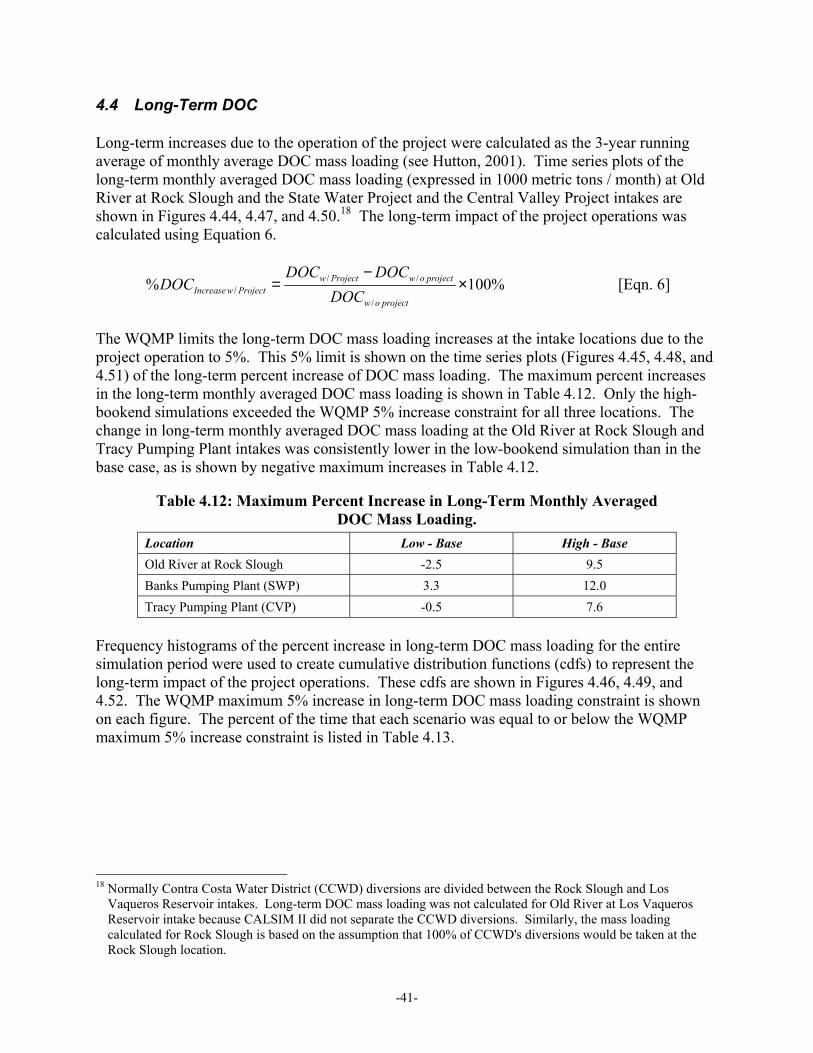
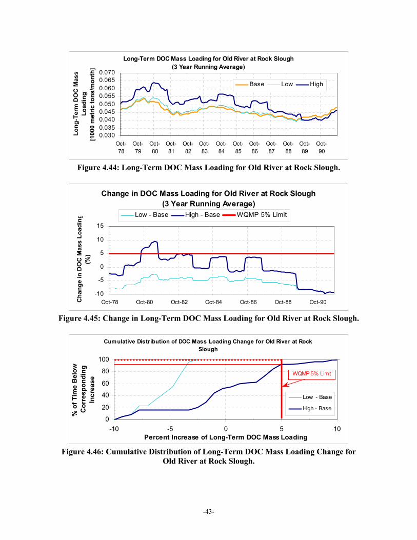
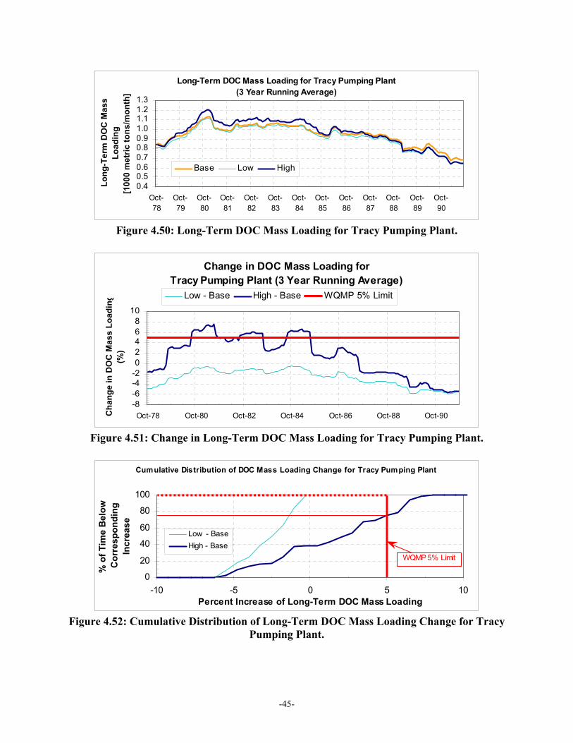
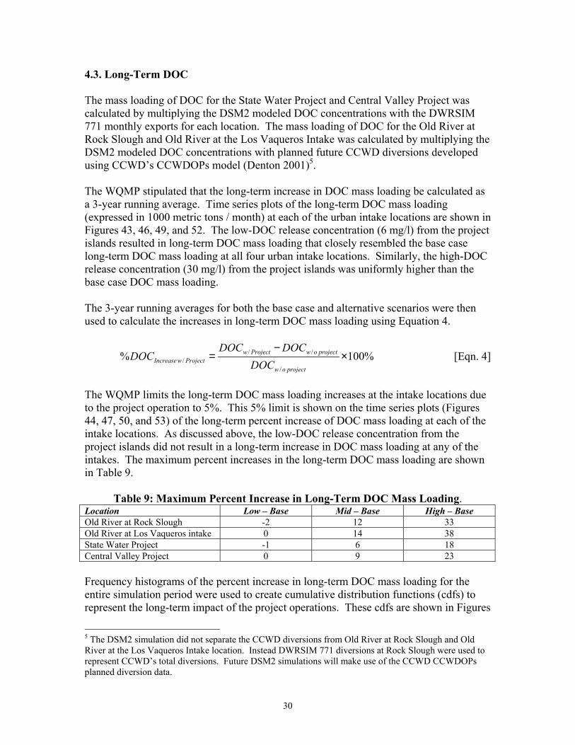
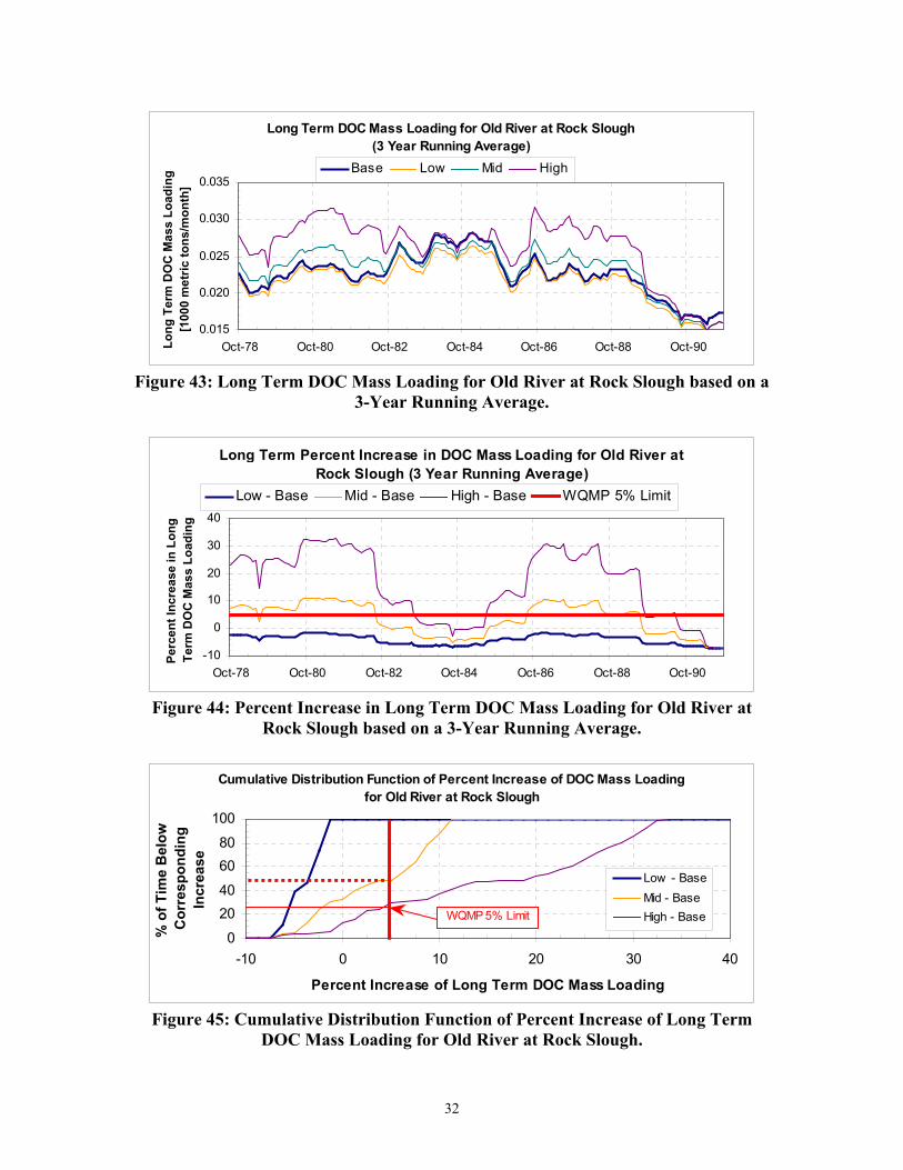
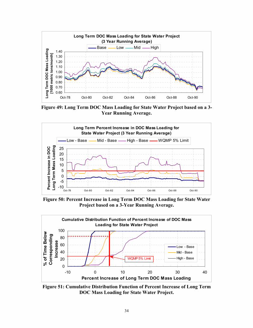
4.4 Long-Term DOC Long-term increases due to the operation of the project were calculated as the 3-year running average of monthly average DOC mass loading (see Hutton, 2001). Time series plots of the long-term monthly averaged DOC mass loading (expressed in 1000 metric tons / month) at Old River at Rock Slough and the State Water Project and the Central Valley Project intakes are shown in Figures 4.44, 4.47, and 4.50.18 The long-term impact of the project operations was calculated using Equation 6.

/ //

/


w o project

DOC DOCDOC

DOC−

= × [Eqn. 6]

The WQMP limits the long-term DOC mass loading increases at the intake locations due to the project operation to 5%. This 5% limit is shown on the time series plots (Figures 4.45, 4.48, and 4.51) of the long-term percent increase of DOC mass loading. The maximum percent increases in the long-term monthly averaged DOC mass loading is shown in Table 4.12. Only the high-bookend simulations exceeded the WQMP 5% increase constraint for all three locations. The change in long-term monthly averaged DOC mass loading at the Old River at Rock Slough and Tracy Pumping Plant intakes was consistently lower in the low-bookend simulation than in the base case, as is shown by negative maximum increases in Table 4.12.

Table 4.12: Maximum Percent Increase in Long-Term Monthly Averaged DOC Mass Loading.

Location Low - Base High - Base Old River at Rock Slough -2.5 9.5 Banks Pumping Plant (SWP) 3.3 12.0 Tracy Pumping Plant (CVP) -0.5 7.6

Frequency histograms of the percent increase in long-term DOC mass loading for the entire simulation period were used to create cumulative distribution functions (cdfs) to represent the long-term impact of the project operations. These cdfs are shown in Figures 4.46, 4.49, and 4.52. The WQMP maximum 5% increase in long-term DOC mass loading constraint is shown on each figure. The percent of the time that each scenario was equal to or below the WQMP maximum 5% increase constraint is listed in Table 4.13.

18 Normally Contra Costa Water District (CCWD) diversions are divided between the Rock Slough and Los

Vaqueros Reservoir intakes. Long-term DOC mass loading was not calculated for Old River at Los Vaqueros Reservoir intake because CALSIM II did not separate the CCWD diversions. Similarly, the mass loading calculated for Rock Slough is based on the assumption that 100% of CCWD's diversions would be taken at the Rock Slough location.

-41-

Table 4.13: Percent Time that the Percent Increase of Long-Term DOC Mass Loading Exceeds the WQMP Maximum 5% Increase Constraint.

Location % Exceedance Low - Base

% Exceedance High - Base

Old River at Rock Slough 0 8 Banks Pumping Plant (SWP) 0 50 Tracy Pumping Plant (CVP) 0 25

The total number of months, out of the 156 months simulated, that the long-term increase in DOC mass loading exceeds the WQMP5% maximum increase constraint is shown below in Table 4.14.19 None of the three intake locations exceeded the 5% increase constraint for the low-bookend. For the high-bookend, all three locations exceeded the 5% increase constraint. The Banks Pumping Plant exceeded the constraint 50 months, the most for any intake location.

Table 4.14: Number of Months that the Increase in Long-Term DOC Mass Loading

Exceeds the WQMP 5% Increase. Location # Months

Low - Base # Months

High - Base Old River at Rock Slough 0 12 Banks Pumping Plant (SWP) 0 78 Tracy Pumping Plant (CVP) 0 39

19 Instead of 192 months, the long-term mass loading calculations used the first 36 months to calculate the running

average, thus long-term violations come from a sample of only 156 months.

-42-

Long-Term DOC Mass Loading for Old River at Rock Slough(3 Year Running Average)

0.0300.0350.0400.0450.0500.0550.0600.0650.070

Oct-78

Oct-79

Oct-80

Oct-81

Oct-82

Oct-83

Oct-84

Oct-85

Oct-86

Oct-87

Oct-88

Oct-89

Oct-90

Long

-Ter

m D

OC

Mas

s Lo

adin

g[1

000

met

ric to

ns/m

onth

]Base Low High

Figure 4.44: Long-Term DOC Mass Loading for Old River at Rock Slough.

Change in DOC Mass Loading for Old River at Rock Slough (3 Year Running Average)

-10

-5

0

5

10

15

Oct-78 Oct-80 Oct-82 Oct-84 Oct-86 Oct-88 Oct-90Cha

nge

in D

OC

Mas

s Lo

adin

g(%

)

Low - Base High - Base WQMP 5% Limit

Figure 4.45: Change in Long-Term DOC Mass Loading for Old River at Rock Slough.

Cumulative Distribution of DOC Mass Loading Change for Old River at Rock

Slough

0

20

40

60

80

100

-10 -5 0 5 10Percent Increase of Long-Term DOC Mass Loading

% o

f Tim

e B

elow

C

orre

spon

ding

In

crea

se

Low - Base

High - Base

WQMP 5% Limit

Figure 4.46: Cumulative Distribution of Long-Term DOC Mass Loading Change for Old River at Rock Slough.

-43-

Long-Term DOC Mass Loading for Banks Pumping Plant(3 Year Running Average)

0.0

0.5

1.0

1.5

2.0

Oct-78

Oct-79

Oct-80

Oct-81

Oct-82

Oct-83

Oct-84

Oct-85

Oct-86

Oct-87

Oct-88

Oct-89

Oct-90

Long

-Ter

m D

OC

Mas

s Lo

adin

g[1

000

met

ric to

ns/m

onth

]Base Low High

Figure 4.47: Long-Term DOC Mass Loading for Banks Pumping Plant.

Change in DOC Mass Loading forBanks Pumping Plant (3 Year Running Average)

-10

-5

0

5

10

15


nge

in D

OC

Mas

s Lo

adin

g(%

)


Figure 4.48: Change in Long-Term DOC Mass Loading for Banks Pumping Plant.

Cumulative Distribution of DOC Mass Loading Change for Banks Pumping Plant

0

20

40

60

80

100


% o

f Tim

e B

elow

C

orre

spon

ding

In

crea

se

Low - BaseHigh - Base

WQMP 5% Limit

Figure 4.49: Cumulative Distribution of Long-Term DOC Mass Loading Change for Banks Pumping Plant.

-44-

Long-Term DOC Mass Loading for Tracy Pumping Plant(3 Year Running Average)

0.40.50.60.70.80.91.01.11.21.3

Oct-78

Oct-79

Oct-80

Oct-81

Oct-82

Oct-83

Oct-84

Oct-85

Oct-86

Oct-87

Oct-88

Oct-89

Oct-90

Long

-Ter

m D

OC

Mas

s Lo

adin

g[1

000

met

ric to

ns/m

onth

]

Base Low High

Figure 4.50: Long-Term DOC Mass Loading for Tracy Pumping Plant.

Change in DOC Mass Loading forTracy Pumping Plant (3 Year Running Average)

-8-6-4-202468

10


nge

in D

OC

Mas

s Lo

adin

g(%

)


Figure 4.51: Change in Long-Term DOC Mass Loading for Tracy Pumping Plant.

Cumulative Distribution of DOC Mass Loading Change for Tracy Pumping Plant

0

20

40

60

80

100


% o

f Tim

e B

elow

C

orre

spon

ding

In

crea

se

Low - BaseHigh - Base

WQMP 5% Limit

Figure 4.52: Cumulative Distribution of Long-Term DOC Mass Loading Change for Tracy Pumping Plant.

-45-

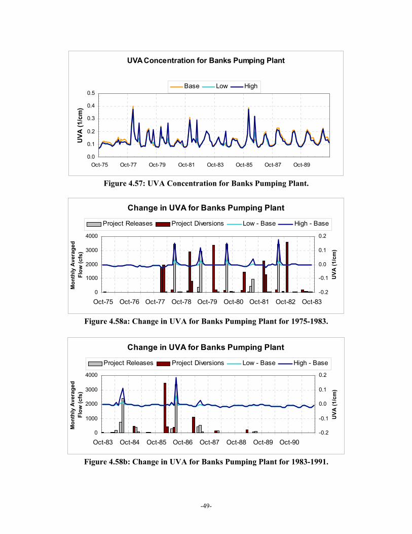
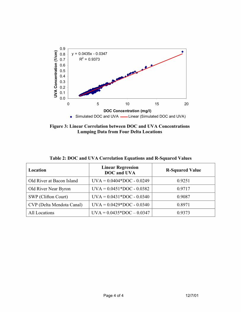
4.5 UVA Like DOC, storage in a Delta reservoir for several months should increase the UVA measurements. Since the growth formulation modifications made to QUAL only applied to DOC, the UVA results presented here were calculated from the QUAL DOC simulations (see Section 4.3), which accounted for the growth of DOC due to long storage times. Previous work relating DSM2 DOC to UVA results has shown that there is a strong relationship between modeled DOC and UVA at the four intake locations (Anderson, 2001). Anderson developed a linear regression (Equation 7) that was used in this report to convert both the low- and high-bookend DOC results at the four urban intakes to equivalent UVA values.

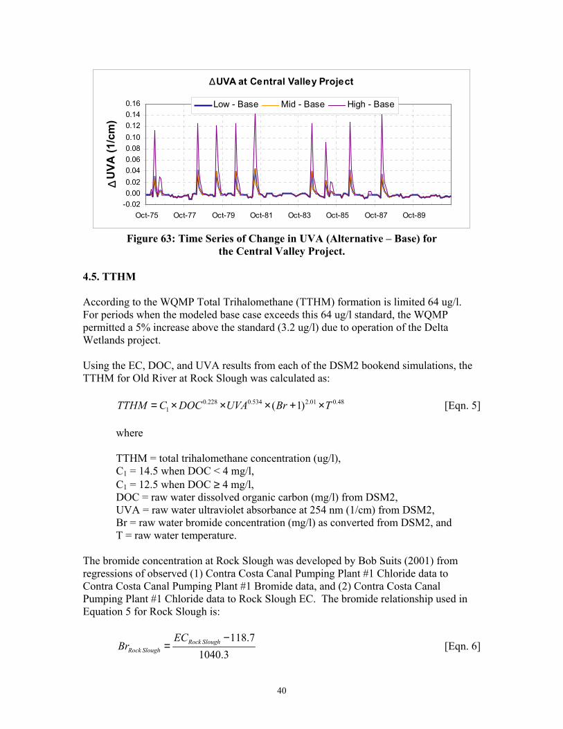
0.0435 0.0347UVA DOC= × − [Eqn. 7] Figures 4.53, 4.55, 4.57, and 4.59 illustrate the sensitivity to UVA release at each of the four urban intake locations: Old River at Rock Slough, Old River at the Los Vaqueros Intake, the State Water Project intake at Banks Pumping Plant, and the Central Valley Project intake at Tracy. In the base case, the periods of high UVA for all of the locations coincided with the high runoff periods that start in the late winter and last through the spring. The maximum monthly averaged UVA for each location is shown in Table 4.15. Both the time series plots and Table 4.15 show that the operation of the project resulted in lower maximum monthly averaged UVA values at the intake locations for the low- and high-bookend simulations.

Table 4.15: Maximum Monthly Averaged UVA (cm-1). Location Base Low Bookend High Bookend Old River at Rock Slough 0.33 0.30 0.30 Old River at Los Vaqueros Intake 0.35 0.32 0.32 Banks Pumping Plant (SWP) 0.40 0.38 0.38 Tracy Pumping Plant (CVP) 0.42 0.40 0.40

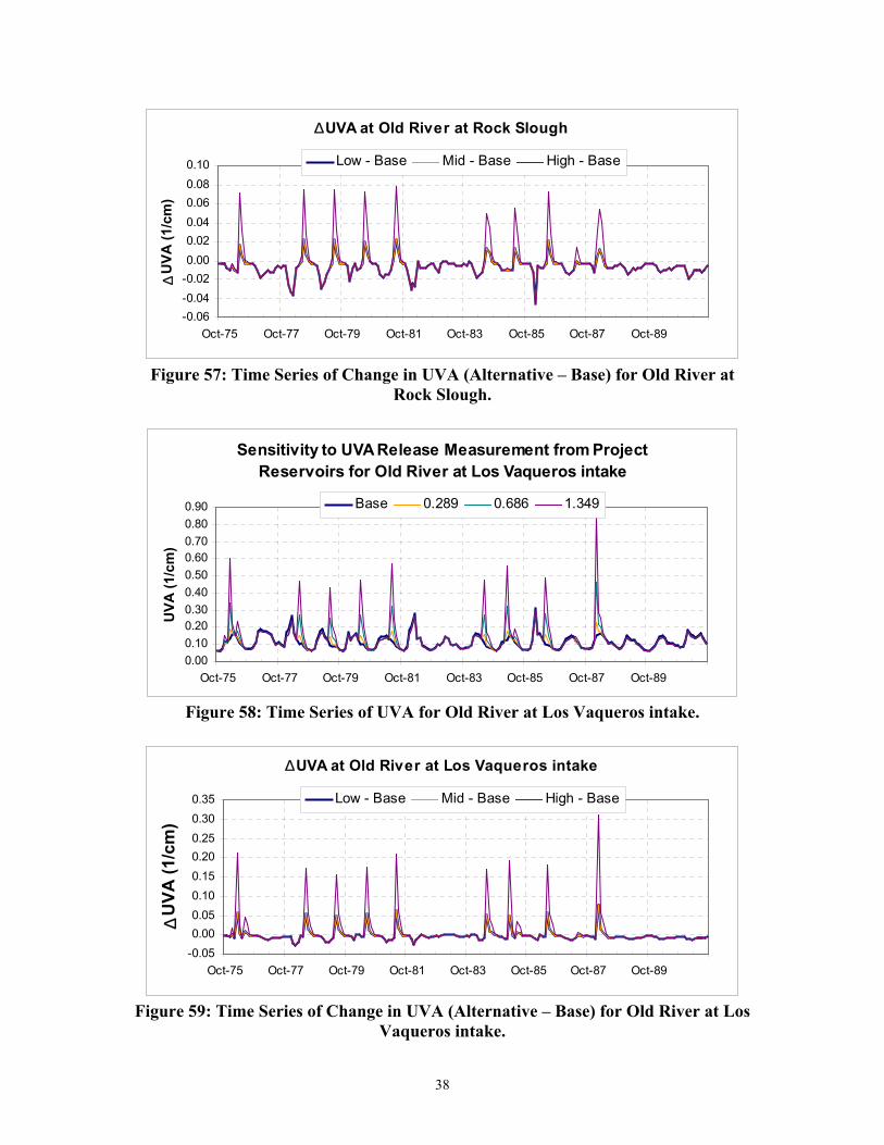
Figures 4.54, 4.56, 4.58, and 4.60 allow a closer look at the changes between the alternative simulation and the base case simulations. In addition to showing the time series of change between the alternative and base case, the combined project releases and diversions are also plotted. Summer time releases from the project increased the UVA concentration by more than 0.1 cm-1 for the high-bookend simulation during 6 of the 8 release periods at all four intake locations. The two remaining periods (summers of 1981 and 1987) had substantially lower project releases. The maximum monthly averaged increase in UVA at each of the intake locations is shown in Table 4.16. The smallest increase in UVA due to project operation occurred at Old River at Rock Slough. The largest increases in UVA were at Banks and Tracy.

Table 4.16: Maximum Monthly Averaged Increase in UVA (cm-1). Location Low - Base High - Base Old River at Rock Slough 0.03 0.13 Old River at Los Vaqueros Intake 0.04 0.16 State Water Project 0.06 0.19 Central Valley Project 0.06 0.18

-46-

UVA Concentration for Old River at Rock Slough

0.000.050.100.150.200.250.300.35


UVA

(1/c

m)

Base Low High

Figure 4.53: UVA Concentration for Old River at Rock Slough.

Change in UVA for Old River at Rock Slough

0

1000

2000

3000

4000


Mon

thly

Ave

rage

d Fl

ow

(cfs

)

-0.2

-0.1

0.0

0.1

0.2

UVA

(1/c

m)

Project Releases Project Diversions Low - Base High - Base

Figure 4.54a: Change in UVA for Old River at Rock Slough for 1975-1983.

Change in UVA for Old River at Rock Slough

0

1000

2000

3000

4000


Mon

thly

Ave

rage

d Fl

ow (c

fs)

-0.2

-0.1

0.0

0.1

0.2

UVA

(1/c

m)


Figure 4.54b: Change in UVA for Old River at Rock Slough for 1983-1991.

-47-

UVA Concentration for Old River at Los Vaqueros Intake

0.000.050.100.150.200.250.300.350.40


UVA

(1/c

m)

Base Low High

Figure 4.55: UVA Concentration for Old River at Los Vaqueros Intake.

Change in UVA for Old River at Los Vaqueros Intake

0

1000

2000

3000

4000


Mon

thly

Ave

rage

d Fl

ow (c

fs)

-0.2

-0.1

0.0

0.1

0.2

UVA

(1/c

m)


Figure 4.56a: Change in UVA for Old River at Los Vaqueros Intake for 1975-1983.

Change in UVA for Old River at Los Vaqueros Intake

0

1000

2000

3000

4000


Mon

thly

Ave

rage

d Fl

ow (c

fs)

-0.2

-0.1

0.0

0.1

0.2

UVA

(1/c

m)


Figure 4.56b: Change in UVA for Old River at Los Vaqueros Intake for 1983-1991.

-48-

UVA Concentration for Banks Pumping Plant

0.0

0.1

0.2

0.3

0.4

0.5


UVA

(1/c

m)

Base Low High

Figure 4.57: UVA Concentration for Banks Pumping Plant.

Change in UVA for Banks Pumping Plant

0

1000

2000

3000

4000


Mon

thly

Ave

rage

d Fl

ow (c

fs)

-0.2

-0.1

0.0

0.1

0.2

UVA

(1/c

m)


Figure 4.58a: Change in UVA for Banks Pumping Plant for 1975-1983.

Change in UVA for Banks Pumping Plant

0

1000

2000

3000

4000


Mon

thly

Ave

rage

d Fl

ow (c

fs)

-0.2

-0.1

0.0

0.1

0.2

UVA

(1/c

m)


Figure 4.58b: Change in UVA for Banks Pumping Plant for 1983-1991.

-49-

UVA Concentration for Tracy Pumping Plant

0.0

0.1

0.2

0.3

0.4

0.5


UVA

(1/c

m)

Base Low High

Figure 4.59: UVA Concentration for Tracy Pumping Plant.

Change in UVA for Tracy Pumping Plant

0

1000

2000

3000

4000


Mon

thly

Ave

rage

d Fl

ow (c

fs)

-0.2

-0.1

0.0

0.1

0.2

UVA

(1/c

m)


Figure 4.60a: Change in UVA for Tracy Pumping Plant for 1975-1983.

Change in UVA for Tracy Pumping Plant

0

1000

2000

3000

4000


Mon

thly

Ave

rage

d Fl

ow (c

fs)

-0.2

-0.1

0.0

0.1

0.2

UVA

(1/c

m)


Figure 4.60b: Change in UVA for Tracy Pumping Plant for 1983-1991.

-50-

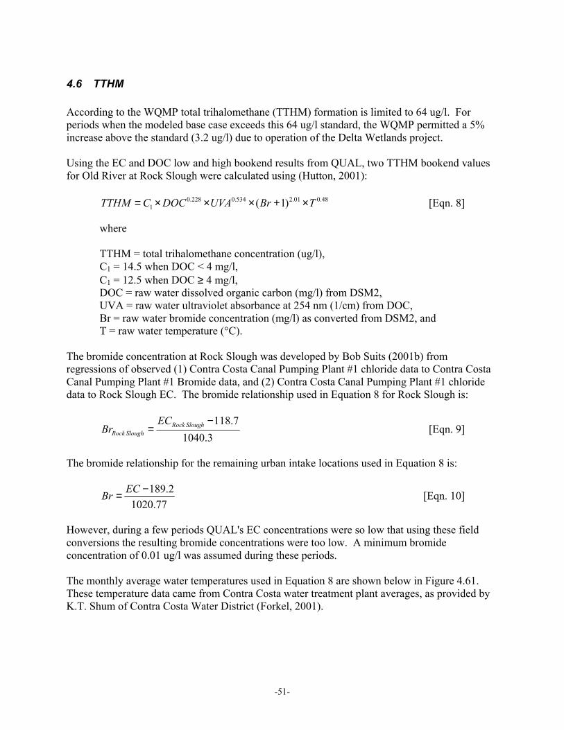
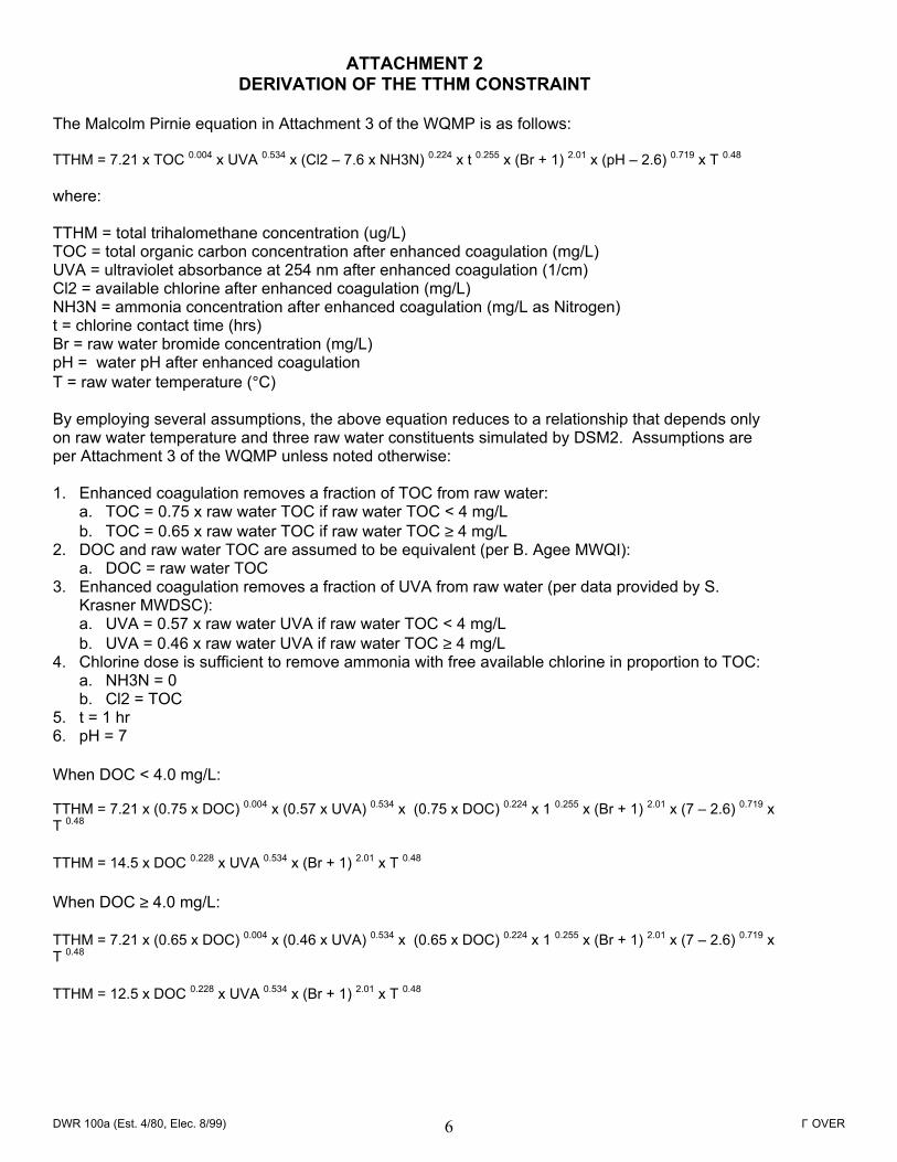
4.6 TTHM According to the WQMP total trihalomethane (TTHM) formation is limited to 64 ug/l. For periods when the modeled base case exceeds this 64 ug/l standard, the WQMP permitted a 5% increase above the standard (3.2 ug/l) due to operation of the Delta Wetlands project. Using the EC and DOC low and high bookend results from QUAL, two TTHM bookend values for Old River at Rock Slough were calculated using (Hutton, 2001): [Eqn. 8] 0.228 0.534 2.01 0.48

1 ( 1)TTHM C DOC UVA Br T= × × × + ×

where TTHM = total trihalomethane concentration (ug/l), C1 = 14.5 when DOC < 4 mg/l, C1 = 12.5 when DOC ≥ 4 mg/l, DOC = raw water dissolved organic carbon (mg/l) from DSM2, UVA = raw water ultraviolet absorbance at 254 nm (1/cm) from DOC, Br = raw water bromide concentration (mg/l) as converted from DSM2, and T = raw water temperature (°C).

The bromide concentration at Rock Slough was developed by Bob Suits (2001b) from regressions of observed (1) Contra Costa Canal Pumping Plant #1 chloride data to Contra Costa Canal Pumping Plant #1 Bromide data, and (2) Contra Costa Canal Pumping Plant #1 chloride data to Rock Slough EC. The bromide relationship used in Equation 8 for Rock Slough is:

118.71040.3

Rock SloughRock Slough

ECBr

−= [Eqn. 9]

The bromide relationship for the remaining urban intake locations used in Equation 8 is:

189.21020.77

ECBr −= [Eqn. 10]

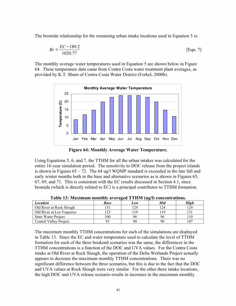
However, during a few periods QUAL's EC concentrations were so low that using these field conversions the resulting bromide concentrations were too low. A minimum bromide concentration of 0.01 ug/l was assumed during these periods. The monthly average water temperatures used in Equation 8 are shown below in Figure 4.61. These temperature data came from Contra Costa water treatment plant averages, as provided by K.T. Shum of Contra Costa Water District (Forkel, 2001).

-51-

Monthly Average Water Temperature

0

5

10

15

20

25

Jan Feb Mar Apr May Jun Jul Aug Sep Oct Nov Dec

Tem

pera

ture

(C)

Figure 4.61: Monthly Average Water Temperature.

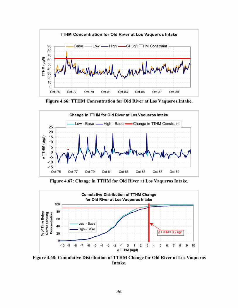
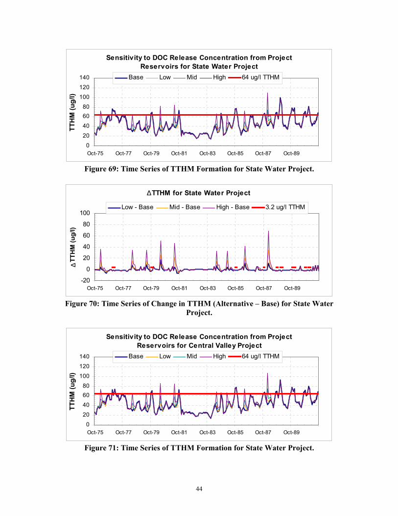
Using Equations 8, 9, and 10, the TTHM for all the urban intakes was calculated for the entire 16-year simulation period. The sensitivity to DOC and bromide release from the project islands is shown in Figures 4.63, 4.66, 4.69, and 4.72. The 64 ug/l WQMP constraint was exceeded only a few times. The base case exceeded this standard in February 1991 at Old River at Rock Slough. At the Old River at Los Vaqueros Intake, Banks, and Tracy, the only time the base case exceeded the TTHM constraint was in March 1977. Both the bromide and DOC were fairly high during this month. Releases from the projects in both alternatives resulted in increases in TTHM, however, the operation of the project also resulted in some slight reductions in the simulated TTHM concentration. For example, though the base case exceeded the 64 ug/l standard in March 1977 at Banks, both the low- and high-bookend simulations were slightly below this constraint. The maximum monthly TTHM concentrations for each of the simulations are displayed in Table 4.17. The largest maximum monthly averaged TTHM concentrations for the base case and low- and high-bookend simulations occurred at Tracy in March 1977. Though the maximum monthly TTHM concentration was the same for the low- and high-bookend simulations at Old River at Rock Slough, the Old River at Los Vaqueros Intake, and the Tracy, as was shown in Figures 4.63, 4.66, 4.69, and 4.72, TTHM was different at other times. The high-bookend maximum monthly averaged TTHM concentration for Banks corresponded with a project release month in July 1986.

Table 4.17: Maximum Monthly Averaged TTHM (ug/l). Location Base Low Bookend High Bookend Old River at Rock Slough 66.8 57.5 57.5 Old River at Los Vaqueros Intake 79.5 68.3 68.3 Banks Pumping Plant (SWP) 67.0 63.9 64.4 Tracy Pumping Plant (CVP) 84.4 82.0 82.0

Time series plots (see Figures 4.64, 4.67, 4.70, 4.73) illustrating the change between each alternative scenario and the base case provide a more useful tool to assess the impact of the project operation on TTHM formation. Although these plots show the change due to the project

-52-

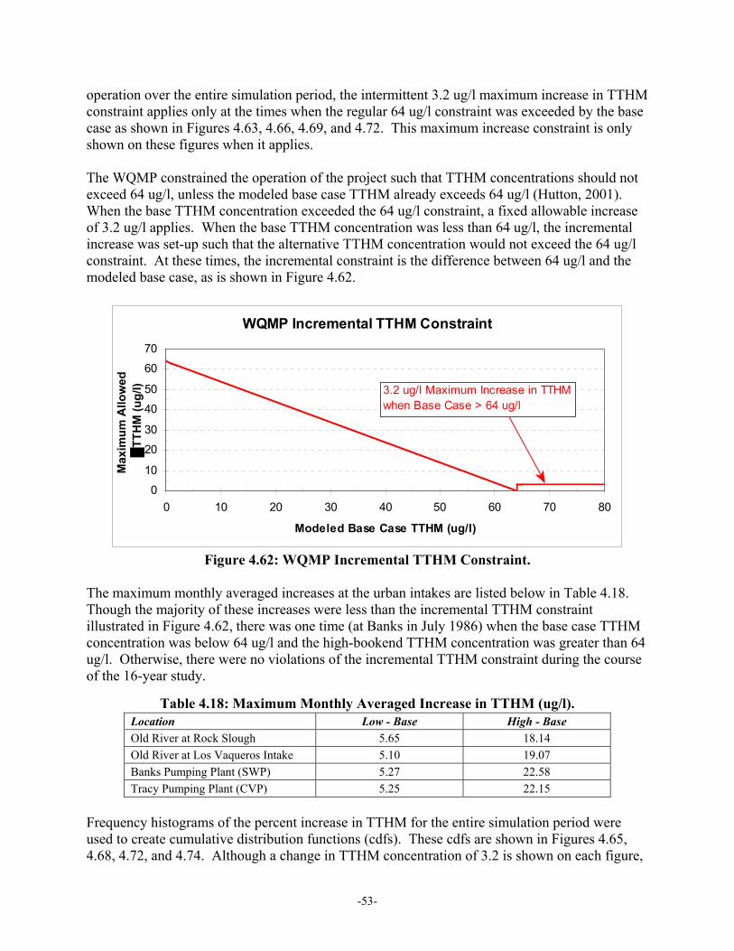
operation over the entire simulation period, the intermittent 3.2 ug/l maximum increase in TTHM constraint applies only at the times when the regular 64 ug/l constraint was exceeded by the base case as shown in Figures 4.63, 4.66, 4.69, and 4.72. This maximum increase constraint is only shown on these figures when it applies. The WQMP constrained the operation of the project such that TTHM concentrations should not exceed 64 ug/l, unless the modeled base case TTHM already exceeds 64 ug/l (Hutton, 2001). When the base TTHM concentration exceeded the 64 ug/l constraint, a fixed allowable increase of 3.2 ug/l applies. When the base TTHM concentration was less than 64 ug/l, the incremental increase was set-up such that the alternative TTHM concentration would not exceed the 64 ug/l constraint. At these times, the incremental constraint is the difference between 64 ug/l and the modeled base case, as is shown in Figure 4.62.

WQMP Incremental TTHM Constraint

010

2030

4050

6070

0 10 20 30 40 50 60 70 80

Modeled Base Case TTHM (ug/l)

Max

imum

Allo

wed

TT

HM

(ug/

l)

3.2 ug/l Maximum Increase in TTHMwhen Base Case > 64 ug/l

Figure 4.62: WQMP Incremental TTHM Constraint. The maximum monthly averaged increases at the urban intakes are listed below in Table 4.18. Though the majority of these increases were less than the incremental TTHM constraint illustrated in Figure 4.62, there was one time (at Banks in July 1986) when the base case TTHM concentration was below 64 ug/l and the high-bookend TTHM concentration was greater than 64 ug/l. Otherwise, there were no violations of the incremental TTHM constraint during the course of the 16-year study.

Table 4.18: Maximum Monthly Averaged Increase in TTHM (ug/l). Location Low - Base High - Base Old River at Rock Slough 5.65 18.14 Old River at Los Vaqueros Intake 5.10 19.07 Banks Pumping Plant (SWP) 5.27 22.58 Tracy Pumping Plant (CVP) 5.25 22.15

Frequency histograms of the percent increase in TTHM for the entire simulation period were used to create cumulative distribution functions (cdfs). These cdfs are shown in Figures 4.65, 4.68, 4.72, and 4.74. Although a change in TTHM concentration of 3.2 is shown on each figure,

-53-

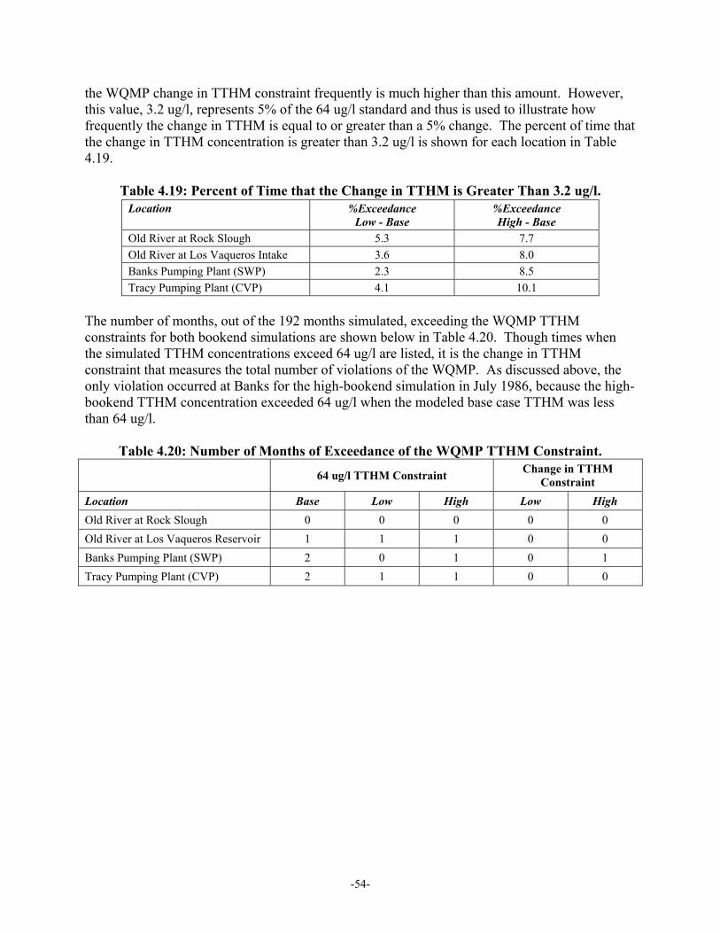
the WQMP change in TTHM constraint frequently is much higher than this amount. However, this value, 3.2 ug/l, represents 5% of the 64 ug/l standard and thus is used to illustrate how frequently the change in TTHM is equal to or greater than a 5% change. The percent of time that the change in TTHM concentration is greater than 3.2 ug/l is shown for each location in Table 4.19.

Table 4.19: Percent of Time that the Change in TTHM is Greater Than 3.2 ug/l. Location %Exceedance

Low - Base %Exceedance High - Base

Old River at Rock Slough 5.3 7.7 Old River at Los Vaqueros Intake 3.6 8.0 Banks Pumping Plant (SWP) 2.3 8.5 Tracy Pumping Plant (CVP) 4.1 10.1

The number of months, out of the 192 months simulated, exceeding the WQMP TTHM constraints for both bookend simulations are shown below in Table 4.20. Though times when the simulated TTHM concentrations exceed 64 ug/l are listed, it is the change in TTHM constraint that measures the total number of violations of the WQMP. As discussed above, the only violation occurred at Banks for the high-bookend simulation in July 1986, because the high-bookend TTHM concentration exceeded 64 ug/l when the modeled base case TTHM was less than 64 ug/l.

Table 4.20: Number of Months of Exceedance of the WQMP TTHM Constraint. 64 ug/l TTHM Constraint Change in TTHM

Constraint Location Base Low High Low High Old River at Rock Slough 0 0 0 0 0 Old River at Los Vaqueros Reservoir 1 1 1 0 0 Banks Pumping Plant (SWP) 2 0 1 0 1 Tracy Pumping Plant (CVP) 2 1 1 0 0

-54-

TTHM Concentration for Old River at Rock Slough

01020304050607080


TTH

M (u

g/l)

Base Low High 64 ug/l TTHM Constraint

Figure 4.63: TTHM Concentration for Old River at Rock Slough.

Change in TTHM for Old River at Rock Slough

-15-10-505

101520


∆TT

HM

(ug/

l)

Low - Base High - Base Change in TTHM Constraint

Figure 4.64: Change in TTHM for Old River at Rock Slough.

Cumulative Distribution of TTHM Changefor Old River at Rock Slough

0

20

40

60

80

100

-10 -9 -8 -7 -6 -5 -4 -3 -2 -1 0 1 2 3 4 5 6 7 8 9 10∆ TTHM (ug/l)

% o

f Tim

e B

elow

C

orre

spon

ding

C

once

ntra

tion

Low - Base

High - Base

∆TTHM = 3.2 ug/l

Figure 4.65: Cumulative Distribution of TTHM Change for Old River at Rock Slough.

-55-

TTHM Concentration for Old River at Los Vaqueros Intake

0102030405060708090


TTH

M (u

g/l)


Figure 4.66: TTHM Concentration for Old River at Los Vaqueros Intake.

Change in TTHM for Old River at Los Vaqueros Intake

-15-10-505

10152025


∆TT

HM

(ug/

l)


Figure 4.67: Change in TTHM for Old River at Los Vaqueros Intake.

Cumulative Distribution of TTHM Changefor Old River at Los Vaqueros Intake

0

20

40

60

80

100

-10 -9 -8 -7 -6 -5 -4 -3 -2 -1 0 1 2 3 4 5 6 7 8 9 10∆ TTHM (ug/l)

% o

f Tim

e B

elow

C

orre

spon

ding

C

once

ntra

tion

Low - Base

High - Base

∆TTHM = 3.2 ug/l

Figure 4.68: Cumulative Distribution of TTHM Change for Old River at Los Vaqueros Intake.

-56-

TTHM Concentration for Banks Pumping Plant

0102030405060708090


TTH

M (u

g/l)


Figure 4.69: TTHM Concentration for Banks Pumping Plant.

Change in TTHM for Tracy Pumping Plant

-15-10-505

10152025


∆TT

HM

(ug/

l)


Figure 4.70: Change in TTHM for Banks Pumping Plant.

Cumulative Distribution of TTHM Changefor Banks Pumping Plant

0

20

40

60

80

100

-10 -9 -8 -7 -6 -5 -4 -3 -2 -1 0 1 2 3 4 5 6 7 8 9 10∆ TTHM (ug/l)

% o

f Tim

e B

elow

C

orre

spon

ding

C

once

ntra

tion

Low - Base

High - Base

∆TTHM = 3.2 ug/l

Figure 4.71: Cumulative Distribution of TTHM Change for Banks Pumping Plant.

-57-

TTHM Concentration for Tracy Pumping Plant

0102030405060708090


TTH

M (u

g/l)


Figure 4.72: TTHM Concentration for Tracy Pumping Plant.

Change in TTHM for Tracy Pumping Plant

-15-10-505

10152025


∆TT

HM

(ug/

l)


Figure 4.73: Change in TTHM for Tracy Pumping Plant.

Cumulative Distribution of TTHM Changefor Tracy Pumping Plant

0

20

40

60

80

100

-10 -9 -8 -7 -6 -5 -4 -3 -2 -1 0 1 2 3 4 5 6 7 8 9 10∆ TTHM (ug/l)

% o

f Tim

e B

elow

C

orre

spon

ding

C

once

ntra

tion

Low - Base

High - Base

∆TTHM = 3.2 ug/l

Figure 4.74: Cumulative Distribution of TTHM Change for Tracy Pumping Plant.

-58-

4.7 Bromate According to the WQMP bromate formation is limited to 8 ug/l. For periods when the modeled base case exceeds this 8 ug/l constraint, the WQMP permitted a 5% increase above the constraint (0.4 ug/l) due to operation of the project. Using EC and DOC discussed in Sections 4.1 and 4.3 above, bromate for all four urban intakes was calculated using (Hutton, 2001):

0.31 0.732BRM C DOC Br= × × [Eqn. 11]

where BRM = bromate (ug/l), C2 = 9.6 when DOC < 4 mg/l, C2 = 9.2 when DOC ≥ 4 mg/l, DOC = raw water dissolved organic carbon (mg/l) from DSM2, and Br = raw water bromide (mg/l) from Equations 8 and 9. The sensitivity of bromate formation potential to project operations is shown in Figures 4.76 - 4.87. Bromate formation is a function of both DOC and bromide concentration. The bromide concentration was calculated based on the EC results discussed in Section 4.1 using Equations 8, 9, and 10 (see Section 4.6). The two DOC bookends modeled were used to calculate two different bromate bookends. Time series plots of the monthly average bromate formation potential at the four intake locations are shown in Figures 4.76, 4.79, 4.82, and 4.85. The base case and alternative simulation bromate formation potentials frequently exceed the 8 ug/l level. The maximum monthly average bromate concentrations for each of the bookend simulations is displayed in Table 4.21. The base case maximum monthly averaged bromate concentrations were higher than both alternative simulation concentrations for all four locations. Tracy had the highest maximum monthly bromate concentration for all three simulations.

Table 4.21: Maximum Monthly Averaged Bromate (ug/l). Location Base Low Bookend High Bookend Old River at Rock Slough 11.67 11.51 11.51 Old River at Los Vaqueros Intake 10.50 10.10 10.10 Banks Pumping Plant (SWP) 11.47 11.30 11.30 Tracy Pumping Plant (CVP) 12.96 12.86 12.86

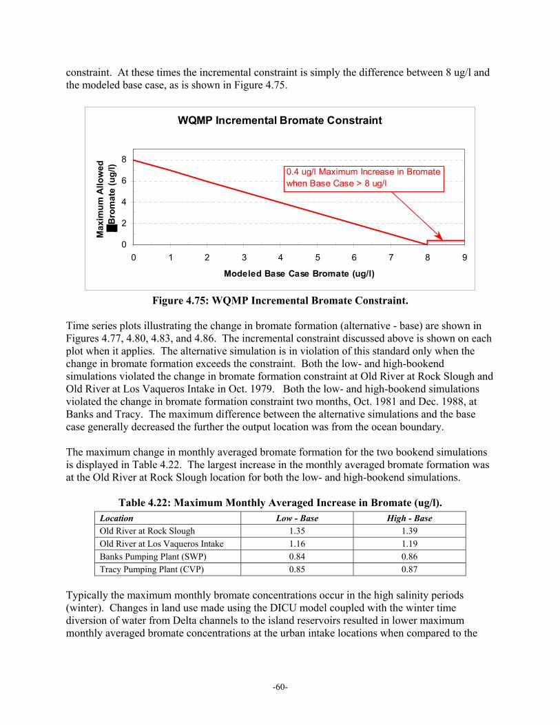
The WQMP constrained the operation of the project such that bromate concentrations should not exceed 8 ug/l, unless the modeled base case bromate already exceeds 8 ug/l (Hutton, 2001). When the base bromate concentration exceeded this constraint, an incremental constraint of 0.4 ug/l applies. When the base bromate concentration was less than 8 ug/l, the incremental increase was set-up such that the alternative bromate concentration would not exceed the 8 ug/l

-59-

constraint. At these times the incremental constraint is simply the difference between 8 ug/l and the modeled base case, as is shown in Figure 4.75.

WQMP Incremental Bromate Constraint

0

2

4

6

8

0 1 2 3 4 5 6 7 8 9

Modeled Base Case Bromate (ug/l)

Max

imum

Allo

wed

B

rom

ate

(ug/

l)

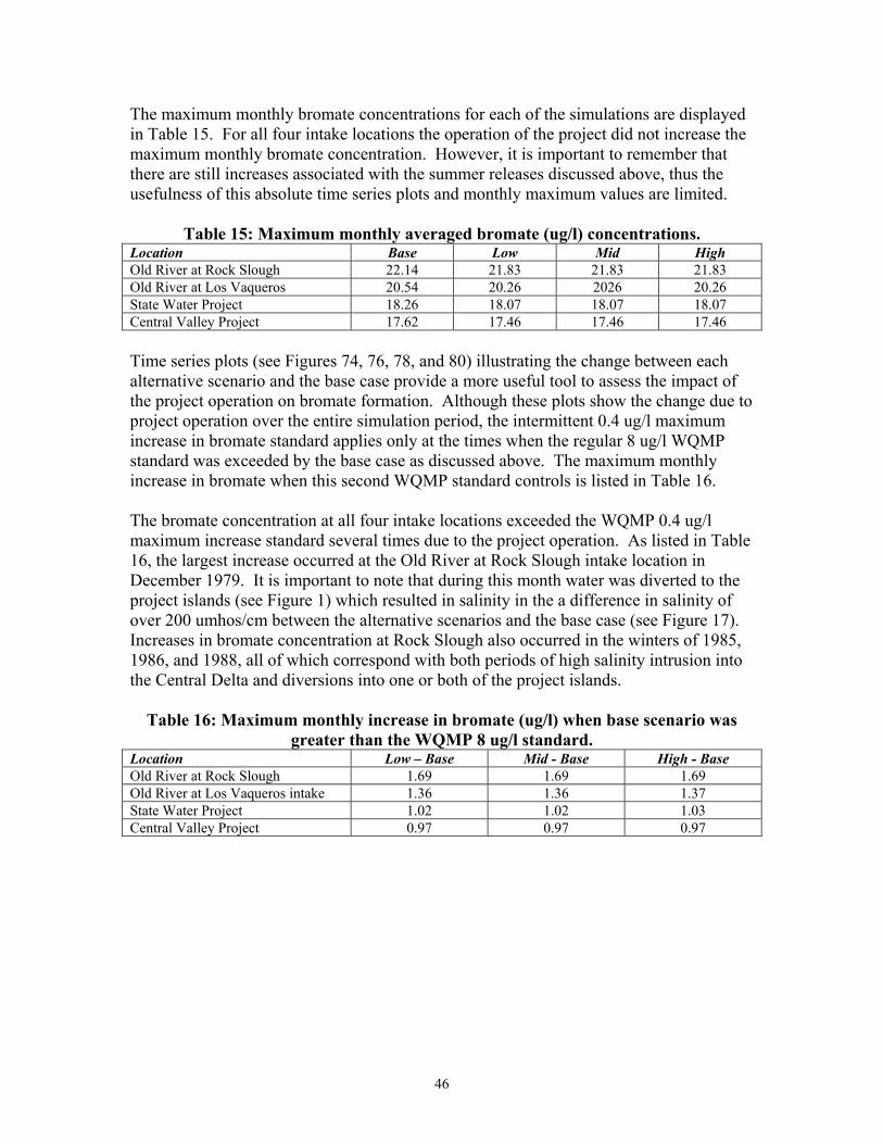
0.4 ug/l Maximum Increase in Bromatewhen Base Case > 8 ug/l

Figure 4.75: WQMP Incremental Bromate Constraint. Time series plots illustrating the change in bromate formation (alternative - base) are shown in Figures 4.77, 4.80, 4.83, and 4.86. The incremental constraint discussed above is shown on each plot when it applies. The alternative simulation is in violation of this standard only when the change in bromate formation exceeds the constraint. Both the low- and high-bookend simulations violated the change in bromate formation constraint at Old River at Rock Slough and Old River at Los Vaqueros Intake in Oct. 1979. Both the low- and high-bookend simulations violated the change in bromate formation constraint two months, Oct. 1981 and Dec. 1988, at Banks and Tracy. The maximum difference between the alternative simulations and the base case generally decreased the further the output location was from the ocean boundary. The maximum change in monthly averaged bromate formation for the two bookend simulations is displayed in Table 4.22. The largest increase in the monthly averaged bromate formation was at the Old River at Rock Slough location for both the low- and high-bookend simulations.

Table 4.22: Maximum Monthly Averaged Increase in Bromate (ug/l). Location Low - Base High - Base Old River at Rock Slough 1.35 1.39 Old River at Los Vaqueros Intake 1.16 1.19 Banks Pumping Plant (SWP) 0.84 0.86 Tracy Pumping Plant (CVP) 0.85 0.87

Typically the maximum monthly bromate concentrations occur in the high salinity periods (winter). Changes in land use made using the DICU model coupled with the winter time diversion of water from Delta channels to the island reservoirs resulted in lower maximum monthly averaged bromate concentrations at the urban intake locations when compared to the

-60-

base case (see Table 4.21). However, the summer releases from the project islands resulted in increases in the monthly averaged bromate concentrations at the urban intakes (see Table 4.22). Frequency histograms of the percent increase in bromate for the entire simulation period were used to create cumulative distribution functions (cdfs). These cdfs are shown in Figures 4.7.3, 4.7.6, 4.7.9, and 4.7.12. Although a change in bromate concentration of 0.4 ug/l is shown on each figure, the WQMP change in bromate formation constraint frequently is much higher than this amount. However, this value, 0.4 ug/l, represents 5% of the 8 ug/l standard and thus is used to illustrate how frequently the change in the bromate formation is equal to or greater than a 5% change. The percent of time that the change in bromate (alternative - base) is greater than this level is shown for each location in Table 4.23.

Table 4.23: Percent of Time that the Change in Bromate is Greater Than 0.4 ug/l. Location %Exceedance

Low - Base %Exceedance High - Base

Old River at Rock Slough 6.3 9.4 Old River at Los Vaqueros Intake 5.7 7.8 Banks Pumping Plant (SWP) 3.6 4.7 Tracy Pumping Plant (CVP) 3.6 4.7

The number of months, out of the 192 months simulated, exceeding the WQMP bromate constraints for both bookend simulations are shown below in Table 4.24. Though the simulated bromate concentration frequently exceeded 8 ug/l, it is the change in bromate constraint that measures the total number of violations of the WQMP. At the two locations closest to the ocean boundary, Old River at Rock Slough and Old River at Los Vaqueros Reservoir, the only violation of the change in bromate constraint occurred in Oct. 1979. Further south, the two violations occurred in Oct. 1981 and Dec. 1988.

Table 4.24: Number of Months of Exceedance of the WQMP Bromate Constraints.

8 ug/l Bromate Constraint Change in Bromate Constraint

Location Base Low High Low High Old River at Rock Slough 46 39 39 1 1 Old River at Los Vaqueros Reservoir 28 25 25 1 1 Banks Pumping Plant (SWP) 24 21 21 2 2 Tracy Pumping Plant (CVP) 26 23 23 2 2

-61-

Bromate Concentration for Old River at Rock Slough

0

2

4

6

8

10

12


Bro

mat

e (u

g/l)

Base Low High 8 ug/l Bromate Constraint

Figure 4.76: Bromate Concentration for Old River at Rock Slough.

Change in Bromate for Old River at Rock Slough

-2

-1

0

1

2


Bro

mat

e (u

g/l)

Low - Base High - Base Change in Bromate Constraint

Figure 4.77: Change in Bromate for Old River at Rock Slough.

Cumulative Distribution of Bromate Changefor Old River at Rock Slough

0

20

40

60

80

100

-1.5 -1.0 -0.5 0.0 0.5 1.0 1.5∆ Bromate (ug/l)

% o

f Tim

e B

elow

C

orre

spon

ding

C

once

ntra

tion

Low - Base

High - Base

∆Bromate = 0.4 ug/l

Figure 4.78: Cumulative Distribution of Bromate Change for Old River at Rock Slough.

-62-

Bromate Concentration for Old River at Los Vaqueros Intake

0

2

4

6

8

10

12


Bro

mat

e (u

g/l)


Figure 4.79: Bromate Concentration for Old River at Los Vaqueros Intake.

Change in Bromate for Old River at Los Vaqueros Intake

-2

-1

0

1

2


Bro

mat

e (u

g/l)


Figure 4.80: Change in Bromate for Old River at Los Vaqueros Intake.

Cumulative Distribution of Bromate Changefor Old River at Los Vaqueros Intake

0

20

40

60

80

100

-1.5 -1.0 -0.5 0.0 0.5 1.0 1.5∆ Bromate (ug/l)

% o

f Tim

e B

elow

C

orre

spon

ding

C

once

ntra

tion

Low - Base

High - Base


Figure 4.81: Cumulative Distribution of Bromate Change for Old River at Los Vaqueros Intake.

-63-

Bromate Concentration for Banks Pumping Plant

0

2

4

6

8

10

12


Bro

mat

e (u

g/l)


Figure 4.82: Bromate Concentration for Banks Pumping Plant.

Change in Bromate for Old River atBanks Pumping Plant

-1.5-1.0-0.50.00.51.01.5


Bro

mat

e (u

g/l)


Figure 4.83: Change in Bromate for Banks Pumping Plant.

Cumulative Distribution of Bromate Changefor Banks Pumping Plant

0

20

40

60

80

100

-1.5 -1.0 -0.5 0.0 0.5 1.0 1.5∆ Bromate (ug/l)

% o

f Tim

e B

elow

C

orre

spon

ding

C

once

ntra

tion

Low - Base

High - Base


Figure 4.84: Cumulative Distribution of Bromate Change for Banks Pumping Plant.

-64-

Bromate Concentration for Tracy Pumping Plant

0

2

4

6

8

10

12


Bro

mat

e (u

g/l)


Figure 4.85: Bromate Concentration for Tracy Pumping Plant.

Change in Bromate for Old River at Tracy Pumping Plant

-1.5-1.0-0.50.00.51.01.5


Bro

mat

e (u

g/l)


Figure 4.86: Change in Bromate for Tracy Pumping Plant.

Cumulative Distribution of Bromate Changefor Old River at Tracy Pumping Plant

0

20

40

60

80

100

-1.5 -1.0 -0.5 0.0 0.5 1.0 1.5∆ Bromate (ug/l)

% o

f Tim

e B

elow

C

orre

spon

ding

C

once

ntra

tion

Low - Base

High - Base


Figure 4.87: Cumulative Distribution of Bromate Change for Tracy Pumping Plant.

-65-

5 Conclusions

The results presented in this study focused primarily on comparing DSM2-QUAL results to the WQMP standards for chloride, DOC, TTHM, and bromate. DSM2-QUAL was modified to account for increases in DOC due to storage. There was no standard for UVA, but the results were shown above since they are used to calculate TTHM. The WQMP constraints apply at any of the urban water supply intakes, thus results were presented for the following locations: Old River at Rock Slough, Old River at the Los Vaqueros Reservoir, the Banks Pumping Plant (SWP), and the Tracy Pumping Plant (CVP) intakes. A summary of the results for each constituent is presented below:

Chloride

WQMP Constraints: Change in Chloride ≤ 10 mg/l, and Chloride (w/ Project) ≤ 225 mg/l.

The base and alternative simulations exceeded 225 mg/l at the Old River at Rock Slough

and Central Valley Project intakes. This constraint was not exceeded at the Old River at Los Vaqueros Reservoir intake and Banks Pumping Plant.

The change in chloride due to operation of the project exceeded 10 mg/l at all four intake

locations with the largest violation occurring at Rock Slough 5.7% of the time.

The percent of time that change in chloride exceeded 10 mg/l ranged between 4 to 6% for the different intake locations.

Long-Term Chloride

WQMP Constraint: Change in Long-Term Chloride Mass Loading ≤ 5%.

The operation of the project exceeded the WQMP 5% long-term increase constraint between 0 to 9% of the time for the three urban intakes.20 The greatest violation occurred at Rock Slough with 14 months exceeding 5%.

The long-term chloride mass loading ranged between 0.7 to 2 thousand metric-

tons/month at Rock Slough, 15 to 28 thousand metric tons/month at Banks, and 11 to 23 thousand metric tons/month at Tracy for both the base and alternative simulations.

20 Old River at Los Vaqueros Reservoir was not calculated because the operations provided by CALSIM II do not

separate the CCWD diversions between Rock Slough and Los Vaqueros.

-66-

DOC

WQMP Constraint: Change in DOC ≤ 1 mg/l.21

The low-bookend island release DOC quality ranged from 6 to 10 mg/l. The high-bookend island releases ranged from 13 to 22 mg/l.

The base and both bookend alternative simulations exceeded 4 mg/l at all four intake locations.

The change in DOC was greater than 1 mg/l at all four intake locations for high-bookend simulations. The change in DOC was greater than 1 mg/l at Banks and Tracy for the low-bookend simulations.

The percent of time that change in DOC exceeded 1 mg/l ranged between 0 to 4% for the

different intake locations.

Long-Term DOC

WQMP Constraint: Change in Long-Term DOC Mass Loading ≤ 5%.

The Banks Pumping Plant exceeded the WQMP 5% long-term increase constraint 0 months for the low-bookend and 78 months for the high-bookend. The Old River at Rock Slough intake exceeded this constraint for only 12 months for the high-bookend simulation.

The operation of the project exceeded the WQMP 5% long-term increase constraint 0% of the time for the three urban intakes for the low-bookend simulation.22 The WQMP 5% long-term increase constraint was exceeded 8 to 50% of the time for the high-bookend simulation.

The long-term DOC mass loading ranged between 0.04 to 0.065 thousand metric-

tons/month at Rock Slough, 0.5 to 1.9 thousand metric tons/month at Banks, and 0.7 to 1.2 thousand metric tons/month at Tracy for both the base and both bookend simulations.

21 The ∆DOC constraint was between 0 and 1 mg/l depending on the modeled base case DOC concentration (see

Hutton, 2001). 22 Old River at Los Vaqueros Reservoir was not calculated because the hydrodynamics provided by CALSIM II do

not separate the CCWD diversions between Rock Slough and Los Vaqueros.

-67-

TTHM

WQMP Constraint: Change in TTHM ≤ 3.2 ug/l.23

The base and both bookend alternative simulations exceeded 64 ug/l at the Old River at Los Vaqueros Reservoir Intake and Tracy. The Banks and Tracy Pumping Plants exceeded the 64 ug/l concentration level for the base case and high-bookend, however, the high-bookend simulation did not increase the TTHM concentration at this time. Old River at Rock Slough did not exceed this concentration for any of the simulations.

The percent of time that the change in TTHM was greater than 3.2 ug/l due to operation of the project ranged between 2 to 5% of the time for the different intake locations for the low-bookend simulation. Similarly, TTHM increased 7.7 to 10% of the time for the high-bookend simulation.

The change in TTHM constraint was violated only once for the high-bookend simulation

at Banks. The rest of the time that the change in TTHM was greater than 3.2 ug/l, the base case was less than 64 ug/l and the alternative did not exceed 64 ug/l.

Bromate

WQMP Constraint: Change in Bromate ≤ 0.4 ug/l.24

The base and both bookend alternative simulations exceeded 8 ug/l at all four intake locations. Rock Slough exceeded this concentration 39 months for both the low- and high-bookend simulations; compared to the 46 months the base case exceeded 8 ug/l at Rock Slough.

The percent of time that the change in bromate was greater than 0.4 ug/l ranged around

6% at Old River at Rock Slough and Old River at Los Vaqueros for the low-bookend. This percentage increased to range between 8 and 9% for the same locations for the high-bookend. However, only one month did these increases result in a violation of the WQMP constraint. The rest of the time that the change in bromate was greater than 0.4 ug/l, the base case was less than 8 ug/l and the alternative did not exceed 8 ug/l.

The percent of time that the change in bromate was greater than 0.4 ug/l at Banks and Tracy was less for both bookend simulations than for the other two locations, however, a total of two months these increases resulted in violations of the WQMP constraint.

23 The ∆TTHM constraint permitted any increase in TTHM when the base case was less than 64 ug/l, otherwise it

limited the ∆TTHM to 5% of 64 ug/l (Hutton, 2001). 24 The ∆Bromate constraint permitted any increase in Bromate when the base case was less than 8 ug/l, otherwise it

limited the ∆Bromate to 5% of 8 ug/l (Hutton, 2001).

-68-

Over the course of the 16-year study, there was a violation of each water quality constraint at least one of the locations for the high-bookend simulations. The low-bookend simulations met the long-term DOC and TTHM constraints at all four locations, however there were violations at some of the locations for all of the other water quality constraints. The most significant violations of the WQMP constraints involved DOC. The Old River at Rock Slough was the only location that did not have a violation in the low-bookend. Out of the eight major release periods, the two Old River locations violated the high-bookend WQMP constraints 6 times, and then the Banks Pumping Plant (SWP) and Tracy Pumping Plant (CVP) violated the WQMP constraints 7 times. There are chloride and bromate violations in the alternative simulations. Although these violations are not directly related to the releases or diversions (meaning they do not always occur during a project release or diversion), they represent a cumulative impact resulting from the re-operation of the entire system in CALSIM. It is important to note that all of the results presented in this report were based on monthly averages. The WQMP actually applies to 14-day running averages. However, the process of averaging water quality results on a monthly basis tended to smooth out peaks in the results. The modifications to QUAL did not account for increases in stored DOC due to primary productivity or due to seepage into the reservoirs from the neighboring channels. Robert Duvall of DWR-ISI is conducting work to study the impact of primary productivity. The violations of the WQMP incremental standards could be minimized by implementing changes in the operation of the project (such as by designing additional operating constraints for CALSIM II to use while modeling the project diversions and releases). Previous DSM2-CALSIM II Delta wetlands studies have shown larger numbers (and magnitudes) of WQMP violations (Mierzwa, 2001). The principle differences between this and previous DSM2 studies are in the CALSIM II operations. One suggested approach to implementing changes in the operation of the project would be to decrease the magnitude of releases from the project islands, but extend the duration of these releases such that a similar volume of water is released.

6 References Anderson, J. (2001). DOC-UVA Correlations. Draft Memo, December 7, 2001. California

Department of Water Resources. Sacramento, CA. Ateljevich, E. (2001a). "Chapter 11: Improving Estimates of Salinity at the Martinez

Boundary." Methodology for Flow and Salinity Estimates in the Sacramento-San Joaquin Delta and Suisun Marsh. 21st Annual Progress Report to the State Water Resources Control Board. California Department of Water Resources. Sacramento, CA.

Ateljevich, E. (2001b). "Chapter 10: Planning Tide at the Martinez Boundary." Methodology

for Flow and Salinity Estimates in the Sacramento-San Joaquin Delta and Suisun Marsh.

-69-

-70-

21st Annual Progress Report to the State Water Resources Control Board. California Department of Water Resources. Sacramento, CA.

Delta Wetlands Water Quality Management Plan. (2000). Exhibit B from the Protest Dismissal

Agreement Between Contra Costa Water District and Delta Wetlands Properties. Easton, D. (2001). CALSIM Model Runs; In-Delta Storage Facilities. Draft Memo, December,

2001. California Department of Water Resources. Sacramento, CA. Forkel, D. (2001). Correspondence about Delta in channel water temperatures for use in

calculating TTHM formation. Hutton, P. (2001). ISI In-Delta Storage: CALSIM Water Quality Constraints to Meet Delta

Wetlands WQMP. Draft Memo, May 29, 2001. California Department of Water Resources. Sacramento, CA.

Jung, M. (2000). Revision of Representative Delta Island Return Flow Quality for DSM2 and

DICU Model Runs, Municipal Water Quality Investigation Program. California Department of Water Resources − Division of Planning and Local Assistance, Sacramento, CA.

Jung, M. (2001a). Reservoir Island Organic Carbon Model: Executive Summary. Draft Report,

November 2001. California Department of Water Resources. Sacramento, CA. Jung, M. (2001b). E-mail correspondence about recommended wetland return water quality

concentrations. Mierzwa, M. (2001). Delta Wetlands Preliminary DSM2 Studies. Memo, August 26, 2001.

California Department of Water Resources. Sacramento, CA. Pandey, G. (2001). Implementation of DOC Growth Module in DSM2-QUAL. Draft Memo,

November 28. California Department of Water Resources. Sacramento, CA. Suits, B. (2001a). Boundary DOC and UVA for DSM2 Planning Studies. Memo, November 19,

2001. California Department of Water Resources. Sacramento, CA. Suits, B. (2001b). Relationships Between EC, Chloride, and Bromide at Delta Export

Locations. Memo, May 29, 2001. California Department of Water Resources. Sacramento, CA.

Department of Water Resources5/18/01DRAFT

1

ISI Water Quality Studies for the In-Delta Storage ProgramDWR Delta Modeling Work Plan

May 2001 Revision #2

CALFED stakeholders were briefed on the proposed work plan on February 13, 2001through the Drinking Water Quality Operations Workgroup. This is a revision to theMarch 19, 2001 draft work plan.

I. DSM2 STUDIES

1. Evaluate Delta Wetlands 2000 Revised EIR/S Operations Studies

Purpose: To evaluate water quality impacts of operating DW Project according toassumptions in EIR/S. Water quality impacts will be measured against the objectivesoutlined in D-1641, D-1643 and the DW Water Quality Management Plan (WQMP).

Description: David Forkel provided us with Jones and Stokes’ base and plan operationsstudy results in Excel format. The base study represents the No Action Alternative andthe plan study represents unlimited South of Delta demand (Scenario #1). Ten DSM2simulations of the period 1976-91 will be conducted, employing the EIR/S hydrology andoperations and bookend water quality assumptions:

Study 1: Base Case (No Action) -- EC Study 2: Base Case (No Action) -- DOC Study 3: Base Case (No Action) -- UV-254 Study 4: DW Operations -- EC Study 5: DW Operations (6 mg/L DOC release) -- DOC Study 6: DW Operations (15 mg/L DOC release) -- DOC Study 7: DW Operations (30 mg/L DOC release) -- DOC Study 8: DW Operations (6 mg/L DOC release) -- UV-254 Study 9: DW Operations (15 mg/L DOC release) -- UV-254 Study 10: DW Operations (30 mg/L DOC release) -- UV-254

Duration: 1 month Expected Start Date: March 2001Expected End Date: April 2001

Product: A memorandum report will be prepared summarizing study assumptions andresults.


2

2. Evaluate In-Delta Storage Alternatives with Reconnaissance-Level Water QualityRules

Purpose: To evaluate water quality impacts of In-Delta Storage alternatives and identifyany violations of WQMP.

Description: Several DSM2 simulations will be conducted, employing Delta hydrologyand operations provided by CALSIM studies. DSM2 simulations will utilize dailychanging Delta hydrology provided by CALSIM and MAY utilize a non-repeating tide(see Task IV-1). DSM2 simulations will utilize an IDS release water quality moduledeveloped in consultation with MWQI staff (see Task IV-2). CALSIM simulations willutilize WQMP constraints developed in Task VI-1 and IDS operations rules developed inTask VI-2. Some iteration in development of IDS operations rules will likely benecessary.

Duration: 6 monthsExpected Start Date: July 2001Expected End Date: January 2002

Product: A draft memorandum report will be prepared summarizing study assumptionsand results.

3. Finalize Analysis of In-Delta Storage Alternatives

Purpose: To refine the evaluation of water quality impacts associated with In-DeltaStorage alternatives.

Description: DSM2 simulations conducted in Task II-2 will be refined utilizing the mostcurrent CALSIM studies. CALSIM operations studies will utilize ANNs trained topredict Delta organic concentrations (see Task V-3).

Duration: 3 monthsExpected Start Date: January 2002Expected End Date: April 2002

Product: A memorandum report will be prepared summarizing study assumptions andresults.

II. DSM2 TOOL AND DATA DEVELOPMENT

1. Develop 16-Year Planning Study Setup With Daily Varying Hydrology/Operationsand Non-Repeating Tide

Purpose: To conduct DSM2 water quality planning studies consistent with CALSIMoutput.


3

Description: DSM2 planning studies utilize CALSIM hydrology and operations as input.In the past, this input has been provided on a monthly time step. As part of the IDSproject, CALSIM will soon be providing Delta hydrology and operations on a daily timestep. It is anticipated that DSM2 will provide more meaningful hydrodynamic and waterquality responses to daily changing hydrology and operations. Several modificationsmust be made to the DSM2 planning study setup to accommodate the additionalCALSIM input data. The DSM2 planning study setup will also be modified toaccommodate a non-repeating tide. In the past, DSM2 planning studies have utilized a25-hour repeating tide. While such an approach is computationally advantageous, it doesnot allow for the evaluation of the spring-neap cycle. The DSM2 non-repeating tide willreflect historical conditions. For example, a 16-year planning study (1976-91) will utilizethe tidal stage as observed at Martinez for every computational time step (i.e. 15 minutes)of the simulation period.

Duration: 4 monthsExpected Start Date: March 2001Expected End Date: July 2001

Product: DSM2 user documentation will be updated.

2. Develop Reservoir Island Release Water Quality Module and Implement in DSM2

Purpose: To simulate water quality changes in In-Delta Storage reservoirs in accordancewith best available science.

Description: MWQI consultants and staff will develop a conceptual model andmathematical relationships to describe changes in water quality IDS reservoirs basedupon experimental data (SMARTS). Explanatory variables may include diversionquality, residence time, season, water level, and soil characteristics. Delta Modeling staffwill collaborate with MWQI staff to develop a water balance module that incorporatesthe concepts and mathematical relationships developed by MWQI. Delta Modeling staffwill develop an appropriate linkage of this module to DSM2. The module could beutilized as a pre-processor or could be dynamically linked to DSM2.

Duration: 4 monthsExpected Start Date: March 2001Expected End Date: July 2001

Product: MWQI staff will prepare a memorandum report, describing model algorithm andassumptions. Delta Modeling staff will update DSM2 user documentation as required.

3. Data Development

Purpose: A variety of data development subtasks must be completed to evaluate IDS on adaily time step with DSM2.


4

• Subtask 3-1 Develop a Data Input Editor -- A tool will be developed to assist in Deltahydrodynamics and water quality time series data visualization, manipulation, andquality control.

Duration: 3 monthsExpected Start Date: January 2001Expected End Date: April 2001

Product: DSM2 user documentation will be updated.

• Subtasks 3-2 Salinity Regression Relationships -- IDS will be operated to meetsalinity D-1641 standards or WQMP constraints for EC, chloride, and bromide.CALSIM and DSM2 simulations will be conducted in EC. Model output will betranslated into chloride and bromide as necessary to compare with standards andconstraints.

Duration: 6 monthsExpected Start Date: July 2001Expected End Date: January 2002

Product: Results will be provided to CALSIM team.

• Subtask 3-3 Real Tide Stage – A 16-year time series of observed tidal stage atMartinez will be developed to use as the downstream boundary condition for DSM2planning studies. Data will be developed at 15-minute intervals. Data fill-inprocedures will be utilized to augment observed data.

Duration: 3 monthsExpected Start Date: March 2001Expected End Date: June 2001

Product: A new data set will be developed and made available through the IEP webpage for public review. This data set would be available for future interagency modelcalibrations and peer reviews.

• Subtask 3-4 Water Temperature Daily Time Series – Predicted TTHM formation aturban intakes is a function of several variables, including water temperature. Oneannual pattern of monthly averages is assumed to represent all urban intakes. Createa smoothed daily time series from the monthly averages.

• Subtask 3-5 Geometry Changes for Alternative 3 – Make necessary geometrychanges in DSM2 input files to represent IDS Alternative 3, which assumes VictoriaIsland as an IDS reservoir.


5

• Task 3-6 Develop Habitat Island Assumptions – Implement appropriate assumptionsfor island diversion volumes, return volumes, and return water quality for habitatislands. Replace assumptions currently in the DICU model for agricultural land use.

• Task 3-7 UVA Conservation – Demonstrate that UVA can be modeled as aconservative constituent. DWR’s Water Quality Assessment staff have been asked toconduct a dilution test to demonstrate.

• Task 3-8 Develop Appropriate Ratios between TOC and DOC. DWR’s WaterQuality Assessment staff has indicted that the DOC:TOC ratio is complex and mayvary temporally and spatially. Assumed ratios may need to account for seasonalvariation. If spatial variation is significant, TOC may need to be simulated directly(instead of DOC).

III. CALSIM ARTIFICIAL NEURAL NETWORK DEVELOPMENT ANDENHANCEMENTS

1. Enhance Existing CALSIM ANN: Phase 1

Purpose: To improve the predictive ability of the existing CALSIM2 ANN.

Description: The CALSIM salinity ANN will be re-trained with data generated by themost recent calibration of DSM2 (2000 IEP PWT calibration). The ANN approach willbe tested for stability under a variety of extreme conditions, including future demand andlevel of development scenarios.

Duration: 2 monthsExpected Start Date: February 2001Expected End Date: April 2001

Product: This task will result in an improved CALSIM ANN module.

2. Enhance Existing CALSIM ANN: Phase 2

Purpose: To add features necessary for evaluating salinity impacts of In-Delta Storagealternatives with daily changing hydrology and non-repeating tide over a 16-yearplanning period.

Description: The CALSIM salinity ANN input structure will be modified to reflectpotential IDS facilities and operations. The ANN will be trained on daily-changinghydrology and operations, and will provide daily average salinity output at current D-1641 locations as well as at IDS diversion points and representative urban intakesspecified in the WQMP.

Duration: 2 monthsExpected Start Date: April 2001


6

Expected End Date: June 2001

Product: This task will result in a CALSIM ANN module that will insure that the IDSmeets salinity objectives outlined in D-1641 and in the WQMP.

3. Develop and Implement New CALSIM ANNs for DOC and UVA

Purpose: To develop an efficient CALSIM module that insures that IDS meetsorganic/DBP objectives outlined in the WQMP.

Description: CALSIM2 will require information on how to operate the In-Delta StorageProject while meeting the WQMP objectives. The operating rules must specify when andhow much water should be diverted into storage or released from storage. CALSIM2 iscurrently provided salinity-based water quality conditions in the Delta through anArtificial Neural Network (ANN) flow-salinity routine. The existing ANN is trained onDSM2 salinity transport simulations. This project will develop new ANNs that provideCALSIM2 with information on organic-based water quality conditions. These newANNs will be trained on DSM2 simulations of dissolved organic carbon (DOC) andultraviolet absorbance (UV-254). It is anticipated that the structure of the organic ANNswill be significantly different from the salinity ANN.

Duration: 7 monthsExpected Start Date: June 2001Expected End Date: January 2002

Product: This task will result in a CALSIM ANN module that will insure that the IDSmeets organic water quality objectives outlined in the WQMP.

IV. CALSIM WATER QUALITY RULES DEVELOPMENT

1. Consult CALSIM Team in Developing Water Quality Constraints

Purpose: To develop CALSIM linear programming constraints that adequately representthe WQMP.

Description: Consult with CALSIM Team to interpret the Delta Wetlands WQMP.Assist in identifying key water quality constraints and formulating representative linearprogramming constraints.

Duration: <1 monthExpected Start Date: March 2001Expected End Date: July 2001

Product: The CALSIM team will develop LP constraints that appropriately represent the WQMP.


7

2-4. Develop Reconnaissance-Level Water Quality Rules for In-Delta StorageOperations

Purpose: To develop simplified CALSIM operating rules that insure that the In-DeltaStorage Project meets organic/DBP objectives outlined in the WQMP.

Description: CALSIM2 will require information on how to operate the In-Delta StorageProject while meeting the WQMP objectives. The operating rules must specify when andhow much water should be diverted into storage or released from storage. CALSIM2 iscurrently provided salinity-based water quality conditions in the Delta through anArtificial Neural Network (ANN) flow-salinity routine. Our intent is to develop newANNs that provide CALSIM2 with information on organic-based water qualityconditions. However, our experience with ANN development indicates that such aproject may extend beyond the timeframe of the Program. Therefore, we intend todevelop simplified operating rules in parallel with ANN development. Simplifiedoperating rules will be developed through a trial-and-error DSM2 simulation approach.The following subtasks are identified:

1. Diversion Rules2. Diversion Water Quality Specification3. Release Rules

Duration: 4 months Expected Start Date: March 2001Expected End Date: July 2001

Product: A draft memorandum report will be prepared summarizing study assumptionsand results.

5. Develop New CALSIM Cross Delta Flow Relationships

Purpose: To develop new CALSIM relationships that estimate flows through the DeltaCross Channel and Georgiana Slough.

Description: The existing relationship, which predicts Cross Delta flow as a function ofSacramento River flow, is inadequate when utilized on a daily time step. A newrelationship will be developed with DSM2 data. The new relationships will be a functionof Sacramento River flow, Mokelumne and Cosumnes Rivers flow, and Yolo Bypassflow.

Duration: <1 monthExpected Start Date: May 2001Expected End Date: June 2001

Product: Multivariate regression equations will be provided to CALSIM team. A draftmemorandum will be prepared summarizing study assumptions and results.

State of California The Resources Agency

M e m o r a n d u m

In-Delta Storage Fingerprinting Memo Page 1 of 35 12/3/01

Date: December 3, 2001

To: Tara Smith

From: Jamie AndersonDelta Modeling Office of SWP PlanningDepartment of Water Resources

Subject: DSM2 Fingerprinting Simulation for the In-Delta Storage Investigations

This memo documents a DSM2 fingerprinting study conducted as part of the In-Delta Storageinvestigations. As part of the analysis of the impacts of the In-Delta Storage alternatives onwater quality concentrations in the Delta, an improved understanding of source and flowcontributions throughout the Delta was desired. Thus, a DSM2 fingerprinting study wasconducted to determine the relative contributions of the system inflows to total flow and waterquality concentrations at selected Delta locations, including the original proposed DeltaWetlands project intake and release locations.

Relative flow contributions from six sources were examined for the time period March 1991through September 1998. The six flow sources examined were the Sacramento River, SanJoaquin River, Martinez, eastside streams, agricultural drains, and the Yolo Bypass. Simulationresults are detailed in this memo for eight selected locations. Four of the analysis locationscorrespond to export locations: Old River Rock Slough, Old River at Highway 4 (Los Vaqueros),Clifton Court Forebay, and the Delta Mendota Canal intake. Four additional analysis locationscorrespond to the intakes for the original Delta Wetlands project: Webb Tract Intakes 1 and 2,and Bacon Island Intakes 1 and 2.

Since high DOC concentrations are typically an issue of concern during wet months, the fingerprinting results were analyzed on a monthly basis. Since DOC concentrations tend to increaseafter major rainfall events, monthly flow contributions for wet and critical years were analyzedseparately. For all eight locations, the Sacramento River provided the major flow contributionduring winters of critical years (56%-95%), and San Joaquin River flow contributions werehighest during January of wet years (15%-62%). During winters of wet years San Joaquin Riverflow contributions increased at all locations, and in fact provided the majority of the flow at boththe Clifton Court Intake and the Delta Mendota Canal. As might be expected based on theirrelative locations, San Joaquin River flow contributions were higher for the Bacon Island intakelocations than for the Webb Tract locations in both wet and critical years. Agricultural drainageflow contributions were less than 6% at all locations except during January of wet years whenthe flow contributions increased up to 14%. Agricultural drainage concentrations were typicallyhigher at the southern locations (the four export locations and at Bacon Island Intake 2) than atthe more northern locations (the Webb Tract intakes and Bacon Island Intake 1).


Finger printing results for flow contributions for the winter months during wet and critical yearswere utilized to estimate ranges of DOC concentrations at the four export locations and at thefour original Delta Wetlands intake locations. During December and January of critical years thehighest average maximum DOC concentrations throughout the system were estimated whenDOC concentrations in the Sacramento River were high since the Sacramento River provided themajor flow contribution during those time periods. During December and January of criticalyears, varying the DOC concentrations in the San Joaquin River and in agricultural drainageproduced minor changes in estimated DOC concentrations except at Clifton Court and the DeltaMendota Canal. This is due to the fact that the Clifton Court and Delta Mendota Canal sites werethe only sites examined where the San Joaquin River made significant flow contributions duringcritical years. Additionally, flow contributions from agricultural drainage were less than 7% atall sites during critical years. In winters of wet years, the highest estimated DOC concentrationswere associated with high DOC concentrations for the major flow contributor at each location(the Sacramento River for the In-Delta Storage and Old River intakes and the San Joaquin Riverfor Clifton Court and the Delta Mendota Canal). In January of wet years, flow contributions fromagricultural drainage increased to levels that produced the highest estimated DOC concentrationsat all locations when the DOC concentrations of the agricultural drainage were high. Thus, a veryhigh source DOC concentration can have a large impact on the total estimated DOC at a givenlocation even if the flow contribution from that source is relatively minor.

In summary, DSM2 finger printing simulations were conducted to analyze the relative flowcontributions of six sources throughout the Delta. Simulation results were examined at fourexport and the four original Delta Wetlands intake locations. Relative flow contributions fromthe six sources were analyzed as time series over the entire simulation period and on a monthlybasis for both wet and critical years. The simulated relative flow contributions were then utilizedto conduct a sensitivity analysis of estimated DOC concentrations at the eight study sites.Typically estimated DOC concentrations were highest when there were high DOC levels in theflow source that provided the major flow contribution for winters of both critical and wet years.However, during January of wet years, flow contributions from agricultural drainage increased tolevels high enough that the highest estimated DOC concentrations were produced when the DOCconcentrations of the agricultural drainage were high. The DSM2 finger printing techniqueprovides a useful tool for sensitivity analysis of boundary condition effects on water quality atselected Delta locations.


Table of ContentsINTRODUCTION....................................................................................................................................................... 5

HYDROLOGY.......................................................................................................................................................... 11

SIMULATION RESULTS ....................................................................................................................................... 11

TIME SERIES OF SIMULATED RESULTS .................................................................................................................... 11COMPARISON OF MONTHLY AVERAGE FLOW CONTRIBUTIONS................................................................................. 12COMPARISON OF FLOW CONTRIBUTIONS DURING WINTER MONTHS FOR WET AND DRY YEARS................................ 12

USE OF FINGER PRINTING TO ESTIMATE DOC CONCENTRATIONS ................................................... 15

SUMMARY-CONCLUSIONS................................................................................................................................. 21

REFERENCES.......................................................................................................................................................... 22

TIME SERIES OF SIMULATION RESULTS ...................................................................................................... 23

MONTHLY AVERAGE SIMULATION RESULTS ............................................................................................ 25

SIMULATION RESULTS FOR WINTERS OF WET AND CRITICAL YEARS ............................................ 28

List of TablesTable 1: Conservative Tracer Constituents Simulated.................................................................... 8

Table 2: Specified Source Tracer Concentations for In-Delta Storage Finger Printing.................. 8

Table 3: Illustrative Examples of Finger Printing Conservative Tracer ConstitutentConcentraitons at Three Locations................................................................................... 9

Table 4: Water Year Designations for 1991-1998 ........................................................................ 11

Table 5: Relative Flow Contributions of the Sacramento River, San Joaquin River andAgricultural Drains during December of Wet and Dry Years ....................................... 14

Table 6: Relative Flow Contributions of the Sacramento River, San Joaquin River andAgricultural Drains during January of Wet and Dry Years ........................................... 14

Table 7: Summary of Average Minimum and Maximum Estimated DOC Concentrations ......... 20

List of FiguresFigure 1: Conceptualization of Relative Source Contributions ...................................................... 5

Figure 2: Proposed In-Delta Storage Alternative 1-Delta Wetlands Project with Original Intakeand Release Locations...................................................................................................... 6

Figure 3: Source Locations for the Validation Fingerprinting Study.............................................. 7

Figure 4: Validation Finger Printing Study Output Locations...................................................... 10

Figure 5: Distribution of Water Year Types for March 1991-September 1998............................ 11


Figure 6: Sample Computations of Estimated DOC Concentrations at Old River at Highway 4 forWet Years....................................................................................................................... 16

Figure 7: Sample Computations of Estimated DOC Concentrations at Old River at Highway 4 forCritical Years ................................................................................................................. 17

Figure 8: Range of Estimated DOC Concentrations for December and January of Wet andCritical Years ................................................................................................................. 19

Figure 9: Time Series of Simulated Relative Contributions of Flow Sources at Delta ExportLocations ........................................................................................................................ 23

Figure 10: Time Series of Simulated Relative Contributions of Flow Sources at the OriginalDelta Wetlands Intake Locations ................................................................................... 24

Figure 11: Monthly Average Simulated Relative Contributions of Flow Sources at Delta ExportLocations for March 1991-September 1998 .................................................................. 26

Figure 12: Monthly Average Simulated Relative Contributions of Flow Sources at the OriginalProposed Delta Wetlands Intake Locations for March 1991-September 1998.............. 27

Figure 13: Simulated Relative Contributions of Flow Sources for Old River at Rock Slough forMarch 1991-September 1998......................................................................................... 28

Figure 14: Simulated Relative Contributions of Flow Sources for Old River at Highway 4 (LosVaqueros) for March 1991-September 1998.................................................................. 29

Figure 15: Simulated Relative Contributions of Flow Sources for Clifton Court Intake for March1991-September 1998 .................................................................................................... 30

Figure 16: Simulated Relative Contributions of Flow Sources for Delta Mendota Canal forMarch 1991-September 1998......................................................................................... 31

Figure 17: Simulated Relative Contributions of Flow Sources for Webb Tract Intake 1 for March1991-September 1998 .................................................................................................... 32

Figure 18: Simulated Relative Contributions of Flow Sources for Webb Tract Intake 2 for March1991-September 1998 .................................................................................................... 33

Figure 19: Simulated Relative Contributions of Flow Sources for Bacon Island Intake 1 forMarch 1991-September 1998......................................................................................... 34

Figure 20: Simulated Relative Contributions of Flow Sources for Bacon Island Intake 2 forMarch 1991-September 1998......................................................................................... 35


IntroductionFor the In-Delta Storage project, DSM2 is being utilized to simulate dissolved organic carbon(DOC) concentrations for both base line and proposed operational alternatives. The proposedDelta Wetlands operational alternatives involve flooding four Delta islands (Figure 2). It isproposed to flood Webb Tract and Bacon Island during high flow periods. These islands wouldbe utilized as in-Delta reservoirs that would provide storage for the water for use during lowerflow periods. Additionally it is proposed to create shallow water habitat in the Delta by floodingBouldin Island and Holland Tract. For this study, the original proposed Delta Wetlands intakeand release locations were used (Figure 2). Later modifications to the proposed intake andrelease locations were not incorporated into this study. As part of the analysis of the impacts ofthe In-Delta Storage alternatives on water quality concentrations in the Delta, an improvedunderstanding of source contributions throughout the Delta was desired. Thus, a DSM2fingerprinting study was conducted to determine the relative contributions of the system inflowsto total flow and water quality concentrations at selected Delta locations.

For this finger printing study, the DSM2 hydrodynamics and water quality validation simulationsconducted by the DWR Delta Modeling Section were utilized as a base case. The validationsimulation was conducted for the time period March 1991 through September 1998. Thehydrology utilized in the validation study included a time varying representation of the tidalboundary at Martinez. For the validation, simulated waterquality constituent concentrations were compared to observedconcentrations. The validation studies are described in moredetail in Nader-Tehrani (2001) and Pandey (2001).

For the validation finger printing study, relative flowcontributions from six sources were examined. The six sourceswere the Sacramento River, San Joaquin River, Martinez,eastside streams, agricultural drains, and the Yolo Bypass.Conceptually the finger printing simulations could be thoughtof as collecting buckets of water from various locationsthroughout the Delta. Each bucket examined would containwater from each source (Figure 1), however the relativecontributions from each source would vary at each location foreach time period that a bucket of water was analyzed.

Figure 1: Conceptualization ofRelative Source Contributions

The relative contributions of each flow source were simulated utilizing seven conservative tracerconstituents denoted as CC1-CC7. Conservative tracer constituents 1 through 6 correspond toindividual source locations (Figure 3). The constituent tracer concentrations were specified as aconstant value at the source location (10,000 units in this case), and a value of zero is specified atall other locations. A seventh conservative tracer constituent is utilized to check massconservation and is specified as the same constant value at each source (10,000 units in thiscase). Source concentrations are specified as 10,000 units to provide large concentrations that


Figure 2: Proposed In-Delta Storage Alternative 1-Delta Wetlands Project with OriginalIntake and Release Locations

Figure adapted from draft document titled “In-Delta StorageProgram: Description of Alternatives” dated 3/6/01

Figure 1IN-DELTA STORAGE

PROGRAMAlternative 1

Lease Delta WetlandsProject

Intake 1

Intake 2

Intake 1

Intake 2


Yolo Bypass

AgriculturalDrains

(250+ locations)

San Joaquin River(Vernalis)

Sacramento River

Martinez

Eastside Streams

Figure 3: Source Locations for the Validation Fingerprinting Study


reduce round-off errors that occur at lower concentrations. Source locations corresponding toeach conservative tracer constituent are indicated in Table 1. Specified concentrations of eachconservative tracer constituent are given in Table 2.

Table 1: Conservative Tracer Constituents Simulated

Source Location Conservative ConstituentSacramento River CC1San Joaquin River CC2Martinez CC3Eastside Streams CC4Agricultural Drains CC5Yolo Bypass CC6All Sources CC7

Table 2: Specified Source Tracer Concentations for In-Delta Storage Finger Printing

Location CC1 CC2 CC3 CC4 CC5 CC6 CC7Sac 10,000 0 0 0 0 0 10,000SJR 0 10,000 0 0 0 0 10,000Martinez 0 0 10,000 0 0 0 10,000Eastside 0 0 0 10,000 0 0 10,000Ag Drains 0 0 0 0 10,000 0 10,000Yolo 0 0 0 0 0 10,000 10,000

If all of the initial conservative constituent tracer concentrations (CC1-CC6) are specified as thesame constant value at the source location associated with each constituent and set equal to zeroat all other source locations, when the system has reached dynamic steady state, the sum of theconcentrations of conservative tracer constituents 1-6 at any location in the system should equalthe specified concentration, 10,000 units in this case. Table 3 shows illustrative finger printingresults for three hypothetical locations. At all three locations, the sum of the concentrations ofconservative tracer constituents 1-6 equals the initial specified concentration of 10,000 units.For location A, the major source of water is the source associated with conservative tracerconstituent 2 (the San Joaquin River-see Table 1) since 3500 units of the 10,000 units totalconcentration was contributed by that source. Similarly the source for conservative tracerconstituent 3 (Martinez) is the major contributor at site B and the source associated withconservative tracer constituent 5 (agricultural drainage) is the main contributor at site C. For theexample illustrated in Table 3, mass is conserved since the concentration of conservative tracerconstituent 7 equals 10,000 units at all locations.


Table 3: Illustrative Examples of Finger Printing Conservative Tracer ConstitutentConcentraitons at Three Locations

Location CC1 CC2 CC3 CC4 CC5 CC6 CC7

A 1000 3500 500 3000 1250 750 10,000

B 2500 500 3000 2000 750 1250 10,000

C 1250 1750 1000 1500 3500 1000 10,000

For the In-Delta Storage finger printing study, the sum of the concentrations of the conservativetracer constituents 1-6 at any specified location equals the initial specified concentration of10,000 units. (Equation 1). The value of conservative tracer constituent 7 at any location in thesystem should also equal the specified concentration as shown in Equation 2. Utilizing a tracerconcentration of 10,000 units for each water source, the relative contribution of a specifiedsource, n, at a given location is given by Equation 3, where CCn is the concentration of theconservative tracer constituent associated with the source n. Note that the relationships specifiedin Equations 1 - 3 are valid for conservative tracer concentrations of 10,000 units at each sourcelocation.

6

110,000

nCCn units

==∑ at any given location in the Delta Eqn. 1

7 10,000CC units= at any given location in the Delta Eqn. 2

Re (%) *100%10,000

CCnlative contribution of source nunits

= Eqn. 3

For this study, twenty eight simulation output locations were chosen to provide a full coveragethroughout the Delta including the intake and release locations for the Delta Wetlands project.The 28 output locations are shown in Figure 4.


15

21

14 17

26

16

5

4

2

2224

2325

27

6

19

20

18

12

13

11

8

1

28

3

7

9

10

Legend1 North Bay Aqueduct2 Sac R @ Greens Lndg3 Steamboat Slough4 Sac R. @ Rio Vista5 Sac R. @ Emmaton6 Mallard Island7 Martinez8 SJR @ Jersey Point9 Webb Tract IDS Intake

Siphon Station 110 Webb Tract IDS Intake

Siphon Station 211 Terminous-Mokelumne R12 Columbia Cut13 Bacon Is. IDS Intake

Siphon Station 1

* IDS=In-Delta Storage

14 Bacon Is. IDS IntakeSiphon Station 2

15 Old River @ Rock Sl16 Contra Costa Intake17 Turner Cut18 Bacon Is. Discharge19 Middle R@Borden Hwy20 North Canal21 Old R. @ Highway 422 Clifton Court Gates23 Delta Mendota Canal24 Grant Line-West End25 Old R. @ Tracy Road26 Middle R. @ Old R.27 SJR @ Brandt Bridge28 SJR @ Vernalis

SJR=San Joaquin River

Figure 4: Validation Finger Printing Study Output Locations


HydrologyThe validation fingerprinting study simulates conditions for the time period March 1991 throughSeptember 1998. The distribution of water year types for this time period are presented in Figure 5and Table 4.

0

1

2

3

4

5

Wet AboveNormal

BelowNormal

Dry Critical

Water Year Type

Num

ber o

f Yea

rs

Figure 5: Distribution of Water Year Types for March 1991-September 1998

Table 4: Water Year Designations for 1991-1998

Water Year SAC 40-30-301991 Critical1992 Critical1993 Above Normal1994 Critical1995 Wet1996 Wet1997 Wet1998 Wet

Simulation ResultsTime Series of Simulated ResultsSimulation results were analyzed at several locations throughout the Delta (Figure 4). Four ofthe analysis locations correspond to export locations: Old River Rock Slough, Old River atHighway 4 (Los Vaqueros), Clifton Court Forebay, and the Delta Mendota Canal intake. Fouradditional analysis locations correspond to the original proposed intakes for the Delta Wetlands


project: Webb Tract Intakes 1 and 2, and Bacon Island Intakes 1 and 2. Time series of relativeflow contributions of the six water sources are shown for the export locations in Figure 9 and forthe original Delta Wetlands intake locations in Figure 10. During dry hydrologic conditions ofthe first several years of the simulation, inflows from the Sacramento River provide the largestflow contribution at all eight locations. During the wetter hydrologic conditions in the last fewyears of the simulation, flow contributions from the San Joaquin River increase. Flowcontributions from agricultural drainage rarely exceed 20% throughout the simulation period atall eight locations.

Comparison of monthly average flow contributionsMonthly distributions of relative flow contributions from six sources over the study period areshown in Figure 11 for the export locations and in Figure 12 for the original proposed DeltaWetlands intake locations. For Rock Slough, Clifton Court Forebay, and the Delta MendotaCanal intake, Sacramento River flows dominate during the summer, fall, and early winter monthswith flow contributions ranging from 40%-90%. However, during the winter and spring, flowcontributions from the San Joaquin River approach and at times exceed those from theSacramento River. At Clifton Court Forebay, flow contributions from the San Joaquin Riverexceed those from the Sacramento River in February through June. For the Old River atHighway 4 site, flow contributions from the San Joaquin River are greater throughout the yearthan for the other three export locations. Similar to the Clifton Court location, flow contributionsfrom the San Joaquin River exceed those of the Sacramento River in February through June. Forboth the Clifton Court and Old River at Highway 4 locations, flow contributions from the SanJoaquin River can exceed 60% during the winter and spring months. Flow contributions fromagricultural drains were highest during the late winter and middle summer months. However, theflow contribution from the agricultural drains never exceeded 15%. All other sourcescontributed less than 10% of the flow in any given month.

For the Delta Wetlands sites, Sacramento River flows typically dominated. For both Webb TractIntake locations, flow contributions from the Sacramento River ranged from 55% to 90% for allmonths. Flow contributions from the San Joaquin River were minor at the Webb Tract intakelocations during the summer and fall months. During the winter and spring months, flowcontributions from the San Joaquin River increased, but never exceeded 40%. Flowcontributions at intake 2 at Bacon Island follow a similar pattern to the Webb Tract intakes.However, intake 1 at Bacon Island shows more influence from the San Joaquin River. Flowcontributions from the San Joaquin are typically less than 20% during the summer and fallmonths, but increase to more than 60% during the winter and spring months. For all four intakelocations, flow contributions from agricultural drains were highest during the late winter andmiddle summer months. However, the total flow contribution from the agricultural drains neverexceeded 15%. All other sources contributed less than 10% of the flow in any given month.

Comparison of flow contributions during winter months for wet and dry yearsSince high DOC concentrations are typically an issue of concern during wet months, the fingerprinting results were analyzed on a monthly basis. Since DOC concentrations tend to increaseafter major rainfall events, the monthly flow contributions for wet and critical years wereanalyzed separately. Relative flow contributions for the months of December and January in wetand dry years are shown for the eight analysis locations in Figure 13 through Figure 20. Relative


flow contributions of the Sacramento River, San Joaquin River, and agricultural drainage duringwet and dry years are summarized in Table 5 for the month of December and in Table 6 for themonth of January.

At Old River at Rock Slough, the wintertime flow contributions of the San Joaquin River aremuch greater during the wet years (15% in December and 29% in January) compared to dryones. For Old River at Rock Slough, San Joaquin River flow contributions are almost negligibleduring the critical years when the Sacramento River flow contributions were 90% or more duringthe winter months. Although wintertime flow contributions from agricultural drainage were lessthan 5% during dry years, these flow contributions exceeded the San Joaquin River’s flowcontributions of less than 2%. The largest flow contributions from agricultural drainage occurredduring January of wet years, when 10% of the flow was provided by agricultural drainage.

A similar pattern of flow contributions results at Old River at Highway 4 (Los Vaqueros). Flowcontributions of the San Joaquin River were much greater during wet years (27% in Decemberand 36% in January) than in dry ones. During critical years, at Old River at Highway 4 the SanJoaquin River contributed only 7% of the flow in December and only 2% of the flow in January.During the critical years, the Sacramento River flows dominated with contributions of 81% and88% in December and January respectively. During wet years, the flow contributions from theSacramento River dropped to 63% and 47% in December and January respectively. Agriculturaldrainage flow contributions during the winter months were typically around 6% except inJanuary of wet years when the contribution increased to 12%.

At the two south Delta export locations, Clifton Court Forebay and the Delta Mendota Canal, themajor flow contribution depended on the year type. During wet years the San Joaquin Riverprovided the majority of the flow at the two export locations, and during dry years theSacramento River contributed the majority of the flow. During wet years, the San Joaquin Rivercontributed 52% and 57% of the flow at the Clifton Court Intake and 55% and 61% of the flowat the Delta Mendota Canal in December and January respectively. However during criticalyears, the Sacramento River provided the majority of the flow at Clifton Court Intake and theDelta Mendota Canal. During critical years Sacramento River flow contributions at CliftonCourt Intake were 64% for both December and January, and flow contributions at Delta MendotaCanal were 56% for both December and January. Agricultural drainage flow contributions atboth locations ranged from 4% to 7% for the winter months except in January of wet years whenflow contributions increased to 10% at the Clifton Court Intake and 13% at the Delta MendotaCanal.

During winters of dry years all four original Delta Wetlands intake locations were dominated bySacramento River flows. For the two Webb Tract intakes and Bacon Island Intake 1,Sacramento River flow contributions exceeded 90% in December and January of critical years.Flow contributions from the Sacramento River during critical years were slightly lower at BaconIsland Intake 2 (the southeastern most intake location) with values of 79% and 88% forDecember and January respectively. During wet years, the main source of flow at each intakelocation is the Sacramento River, but flow contributions are lower than in critical years. At theWebb Tract intakes, the Sacramento River contributes around 84% and 62% of the flow in

In-D

elta

Sto

rage

Fin

gerp

rintin

g M

emo

Page

14

of 3

512

/3/0

1

Tab

le 5

: Rel

ativ

e Fl

ow C

ontr

ibut

ions

of t

he S

acra

men

to R

iver

, San

Joa

quin

Riv

er a

nd A

gric

ultu

ral D

rain

sdu

ring

Dec

embe

r of

Wet

and

Dry

Yea

rs

Loc

atio

nSa

c C

ontr

ibut

ion

Dec

Wet

Yea

rsSJ

R C

ontr

ibut

ion

Dec

Wet

Yea

rsA

g C

ontr

ibut

ions

Dec

Wet

Yea

rsSa

c C

ontr

ibut

ion

Dec

Cri

tical

Yea

rsSJ

R C

ontr

ibut

ion

Dec

Cri

tical

Yea

rsA

g C

ontr

ibut

ions

Dec

Cri

tical

Yea

rs

Old

Riv

er a

t Roc

k Sl

ough

76.2

15.0

5.3

89.8

1.6

3.7

Old

Riv

er a

t Hw

y 4

62.9

27.7

6.1

81.0

6.8

5.9

Clif

ton

Cou

rt In

take

42.0

51.5

3.9

63.7

24.9

5.6

Del

ta M

endo

ta C

anal

38.2

55.2

4.2

55.8

33.7

5.3

Web

b Tr

act I

ntak

e 1

83.0

8.1

3.5

92.9

0.4

2.7

Web

b Tr

act I

ntak

e 2

84.2

6.6

2.9

94.4

0.3

2.3

Bac

on Is

land

Inta

ke 1

78.0

13.3

4.9

90.6

1.2

3.4

Bac

on Is

land

Inta

ke 2

63.0

25.0

6.1

78.8

8.1

5.5

Ligh

t gra

y sh

adin

g in

dica

tes t

he m

ajor

flow

sour

ce a

t the

spec

ified

loca

tion

for t

he sp

ecifi

ed ti

me

perio

d

Tab

le 6

: Rel

ativ

e Fl

ow C

ontr

ibut

ions

of t

he S

acra

men

to R

iver

, San

Joa

quin

Riv

er a

nd A

gric

ultu

ral D

rain

sdu

ring

Jan

uary

of W

et a

nd D

ry Y

ears

Loc

atio

nSa

c C

ontr

ibut

ion

Jan

Wet

Yea

rsSJ

R C

ontr

ibut

ion

Jan

Wet

Yea

rsA

g C

ontr

ibut

ions

Jan

Wet

Yea

rsSa

c C

ontr

ibut

ion

Jan

Cri

tical

Yea

rsSJ

R C

ontr

ibut

ion

Jan

Cri

tical

Yea

rsA

g C

ontr

ibut

ions

Jan

Cri

tical

Yea

rs

Old

Riv

er a

t Roc

k Sl

ough

55.9

29.2

9.6

93.4

0.3

4.1

Old

Riv

er a

t Hw

y 4

47.1

36.4

11.8

87.9

2.3

6.7

Clif

ton

Cou

rt In

take

29.9

56.8

10.1

64.2

26.3

6.8

Del

ta M

endo

ta C

anal

23.2

61.1

13.4

56.2

34.9

6.6

Web

b Tr

act I

ntak

e 1

60.5

22.7

8.0

94.8

0.1

3.2

Web

b Tr

act I

ntak

e 2

63.5

15.0

7.5

95.4

0.1

3.1

Bac

on Is

land

Inta

ke 1

57.3

27.4

9.7

93.7

0.3

3.8

Bac

on Is

land

Inta

ke 2

46.8

30.8

13.6

87.5

2.3

5.9

Ligh

t gra

y sh

adin

g in

dica

tes t

he m

ajor

flow

sour

ce a

t the

spec

ified

loca

tion

for t

he sp

ecifi

ed ti

me

perio

d


December and January. Sacramento River flows are also the major contribution at Bacon Islandduring wet winters, however contributions are greater for the western intake (Intake 1-flowcontributions of 78% in December and 57% in January) than the eastern intake (Intake 2-flowcontributions of 63% in December and 47% in January). At all four intake locations, SanJoaquin River flow contributions are minor during critical years. However the San JoaquinRiver’s flow contributions increased during wet winters. During wet winters at Webb Tract theSan Joaquin River contributes 8% and 7% of the December flows at intakes 1 and 2 respectively.In January the San Joaquin River flow contributions increased to 23% and 15% at intakes 1 and2 respectively. For Bacon Island during wet winters, San Joaquin flow contributions were higherthan at Webb Tract with December flow contributions of 13% and 25% and January flowcontributions of 27% and 31% at intakes 1 and 2 respectively. Wintertime agricultural drainageflow contributions were less than 6% at all intake locations except during January of wet yearswhen agricultural drainage flow contributions increased to about 8% at the Webb Tract intakesand 10% at Bacon Island Intake 1 and 14% at Bacon Island Intake 2.

Use of Finger Printing to Estimate DOC ConcentrationsDOC concentrations can be estimated utilizing the relative flow contributions determined by theDSM2 finger printing analysis. The DOC contribution at a given location from a specifiedsource can be estimated by multiplying the DOC concentration of that source by the percentcontribution of that source at that location. The total DOC concentration at the given locationcan be estimated by summing the estimated DOC contributions from each source (Eqn. 4).

* ReSources

DOC at a location DOC concentration source lative contribution of source= ∑ Eqn. 4

Note that using equation 4 and the relative flow contributions determined using the DSM2fingerprinting analysis provides an estimate of DOC concentrations. This methodology does notaccount for field conditions other than flow rates and source concentrations. The type of fingerprinting used for this analysis indicates the relative contributions of each source to flow at aspecified location, but there is no indication of the temporal distribution of the flow from eachsource. For example, the Sacramento River contribution at any given location may be composedof water that entered the Delta at different times and of different qualities. The analysispresented here considers all of the water contributed from a specified source to have a constantwater quality. Thus affects of antecedent conditions and complex chemical interactions are notaccounted for in this methodology.

To illustrate the use of finger printing results to estimate DOC concentrations, DOCconcentrations were estimated at Old River at Highway 4 (Los Vaqueros) for wet and criticalwinters (Figure 6 and Figure 7 respectively). DOC source concentrations were assumed to be0 mg/l at Martinez, 15 mg/l for the agricultural drainage, 5 mg/l for the San Joaquin River, and3 mg/l for the eastside streams and Yolo Bypass. DOC source concentrations for the SacramentoRiver were varied from 3 mg/l to 6 mg/l to examine the sensitivity of the estimated DOCconcentrations at Old River at Highway 4 to the range of DOC source concentrations typicallyobserved in the Sacramento River. Relative flow contributions were determined from the DSM2fingerprinting analysis. DOC concentrations at Old River at Highway 4 were estimated to rangefrom 4.6 mg/l to 6.0 mg/l during wet years for Sacramento River DOC concentrations of 3 mg/l


Old River at Highway 4 (Los Vaqueros) for Wet YearsSacramento River DOC = 3 mg/l

Source Source DOCConcentration

Relative FlowContribution

DOCContribution

Sac 3 46.4 1.4SJR 5 43.3 2.2Martinez 0 0.2 0.0Eastside 3 3.5 0.1Ag Drains 15 6.3 0.9Yolo 3 0.3 0.0

TOTAL DOC 4.6DOC Contribution = Source DOC concentration * Relative Flow Contribution(%)/100

Old River at Highway 4 (Los Vaqueros) for Wet YearsSacramento River DOC = 6 mg/l



DOCContribution



Figure 6: Sample Computations of Estimated DOC Concentrationsat Old River at Highway 4 for Wet Years


Old River at Highway 4 (Los Vaqueros) for Critical YearsSacramento River DOC = 3 mg/l



DOCContribution



Old River at Highway 4 (Los Vaqueros) for Critical YearsSacramento River DOC = 6 mg/l



DOCContribution



Figure 7: Sample Computations of Estimated DOC Concentrationsat Old River at Highway 4 for Critical Years


and 6 mg/l respectively. Similarly for critical years, DOC concentrations were estimated torange from 4.2 mg/l to 6.5 mg/l for Sacramento River DOC concentrations of 3 mg/l and 6 mg/lrespectively.

Sensitivity of estimated wintertime Delta DOC concentrations to DOC source concentrationsfrom agricultural drainage and the Sacramento and San Joaquin Rivers were examined for eachof the eight output locations. At each location, source DOC concentrations were varied over therange of values observed in the field. Sacramento River DOC concentrations were varied from 3to 6 mg/l, San Joaquin River DOC concentrations were varied from 3 to 9 mg/l, and agriculturaldrainage DOC values were varied from 5 to 35 mg/l. Monthly average DOC concentrations forDecember and January were estimated at each location for each combination of source DOCconcentrations for both wet and critical years.

Figure 8 illustrates ranges of DOC concentrations estimated by varying DOC concentrations atone source (either the Sacramento River, San Joaquin River or agricultural drainage) and holdingall other source DOC concentrations constant at values typically observed in the field. Tosynthesize the analysis results, the eight locations were divided into three groups. Webb Tractintakes 1 and 2 and Bacon Island intakes 1 and 2 were grouped as In-Delta Storage intakes. OldRiver at Rock Slough and Old River at Highway 4 were grouped as Old River intakes. Finally,Clifton Court and Delta Mendota Canal were grouped together. Average minimum andmaximum estimated DOC concentrations for each group were computed for the scenariosvarying the DOC source concentrations (Table 7).

Typically maximum estimated DOC concentrations in December and January were higher duringwet years than during critical years at all locations for the scenarios varying source DOCconcentrations from the Sacramento River, San Joaquin River, and agricultural drainage (Figure8 and Table 7). Minimum estimated DOC concentrations for December and January weresimilar for both wet and critical years.

For December and January of critical years, highest average maximum DOC concentrationsthroughout the system were estimated when DOC concentrations in the Sacramento River werehigh (Figure 8 and Table 7). This is due to the large flow contributions from the Sacramento Riverduring critical years at all of the sites examined (Table 5 and Table 6). During December andJanuary of critical years, varying the DOC concentrations in the San Joaquin River and inagricultural drainage produced minor changes in estimated DOC concentrations except at CliftonCourt and the Delta Mendota Canal. This is due to the fact that the Clifton Court and DeltaMendota Canal sites were the only sites examined where the San Joaquin River made significantflow contributions during critical years (Table 5 and Table 6). Flow contributions fromagricultural drainage were less than 7% at all locations during critical years. Thus, for the In-DeltaStorage and Old River intakes the DOC of the Sacramento River inflows had the largest effect onestimated DOC concentrations for December and January of critical years. However, at CliftonCourt and at the Delta Mendota Canal the ranges of influence on estimated DOC in December ofcritical years were similar for all three inflows examined (Sacramento River, San Joaquin River,and agricultural drainage). In January of critical years, the inflows from the San Joaquin River and

In-D

elta

Sto

rage

Fin

gerp

rintin

g M

emo

Page

19

of 3

512

/3/0

1

Figu

re 8

: Ran

ge o

f Est

imat

ed D

OC

Con

cent

ratio

ns fo

r D

ecem

ber

and

Janu

ary

of W

et a

nd C

ritic

al Y

ears

Dec

embe

r Crit

ical

Yea

rsJa

nuar

y C

ritic

al Y

ears

Dec

embe

r Wet

Yea

rsJa

nuar

y W

et Y

ears

34

56

78

9

Bac

on Is

land

Inta

ke 2

Bac

on Is

land

Inta

ke 1

Web

b Tr

act I

ntak

e 2

Web

b Tr

act I

ntak

e 1

Del

ta M

endo

ta C

anal

Clif

ton

Cou

rt In

take

Old

Riv

er a

t Hw

y 4

Old

Riv

er R

ock

Sl

DO

C C

once

ntra

tion

mg/

lD

OC

Sac

=3-6

SJR

=5 A

g=15

DO

C S

JR=3

-9 S

ac=3

Ag=

15D

OC

AG

=5-3

5 S

ac=3

SJR

=5

34

56

78

9

Bac

on Is

land

Inta

ke 2

Bac

on Is

land

Inta

ke 1

Web

b Tr

act I

ntak

e 2

Web

b Tr

act I

ntak

e 1

Del

ta M

endo

ta C

anal

Clif

ton

Cou

rt In

take

Old

Riv

er a

t Hw

y 4

Old

Riv

er R

ock

Sl

DO

C C

once

ntra

tion

mg/

lD

OC

Sac

=3-6

SJR

=5 A

g=15

DO

C S

JR=3

-9 S

ac=3

Ag=

15D

OC

AG

=5-3

5 S

ac=3

SJR

=5

34

56

78

9

Bac

on Is

land

Inta

ke 2

Bac

on Is

land

Inta

ke 1

Web

b Tr

act I

ntak

e 2

Web

b Tr

act I

ntak

e 1

Del

ta M

endo

ta C

anal

Clif

ton

Cou

rt In

take

Old

Riv

er a

t Hw

y 4

Old

Riv

er R

ock

Sl

DO

C C

once

ntra

tion

mg/

lD

OC

Sac

=3-6

SJR

=5 A

g=15

DO

C S

JR=3

-9 S

ac=3

Ag=

15D

OC

AG

=5-3

5 S

ac=3

SJR

=5

34

56

78

9

Bac

on Is

land

Inta

ke 2

Bac

on Is

land

Inta

ke 1

Web

b Tr

act I

ntak

e 2

Web

b Tr

act I

ntak

e 1

Del

ta M

endo

ta C

anal

Clif

ton

Cou

rt In

take

Old

Riv

er a

t Hw

y 4

Old

Riv

er R

ock

Sl

DO

C C

once

ntra

tion

mg/

lD

OC

Sac

=3-6

SJR

=5 A

g=15

DO

C S

JR=3

-9 S

ac=3

Ag=

15D

OC

AG

=5-3

5 S

ac=3

SJR

=5


Table 7: Summary of Average Minimum and Maximum Estimated DOC Concentrations

Location In-Delta StorageIntakes*

Old RiverIntakes**

Clifton Court andDelta Mendota Canal

Varied DOC Source Sac SJR Ag Sac SJR Ag Sac SJR AgAverage MinimumDOC Dec Critical Yrs 3.4 3.3 3.0 3.5 3.5 3.1 4.2 3.6 3.6

Average MaximumDOC Dec Critical Yrs 6.1 3.5 4.0 6.1 3.7 4.1 5.9 5.3 5.2

Average MinimumDOC Dec Wet Yrs 3.8 3.5 3.3 4.1 3.7 3.5 4.5 3.5 4.1

Average MaximumDOC Dec Wet Yrs 6.1 4.3 4.6 6.2 4.9 5.2 5.7 6.7 5.3

Average MinimumDOC Jan Critical Yrs 3.5 3.4 3.1 3.6 3.6 3.1 4.4 3.8 3.7

Average MaximumDOC Jan Critical Yrs 6.2 3.5 4.3 6.4 3.7 4.7 6.2 5.6 5.7

Average MinimumDOC Jan Wet Yrs 4.6 4.2 3.7 4.9 4.3 3.9 5.6 4.4 4.4

Average MaximumDOC Jan Wet Yrs 6.4 5.6 6.6 6.5 6.3 7.1 6.4 7.9 7.9* In-Delta Storage intakes are Webb Tract intakes 1 and 2 and Bacon Island intakes 1 and 2**Old River intakes are Old River at Rock Slough and Old River at Highway 4

agricultural drainage had the greatest impact on estimated DOC concentrations at Clifton Courtand at the Delta Mendota Canal.

During December and January of wet years, the influence of flow contributions from the SanJoaquin River and agricultural drainage becomes more significant in DOC estimations (Figure 8and Table 7). Similar to the results for critical years, for December of wet years the highestestimated DOC concentrations at the In-Delta Storage and Old River intakes were associatedwith the high DOC concentrations in the Sacramento River since the Sacramento River was themajor flow contributor at those locations during that time period (Table 5). However at CliftonCourt and at the Delta Mendota Canal, the San Joaquin River provided the majority of the flowin December and January of wet years (Table 5), and thus the highest estimated DOCconcentrations at those locations in those months were associated with high DOC levels in theSan Joaquin River. In January of wet years, flow contributions from agricultural drainageincreased at all locations (Table 6) and ranged from 7.5% to 13.6%. Although agriculturaldrainage did not provide the largest flow contribution in January of wet years, the flowcontributions became large enough that the largest estimated DOC values throughout the systemoccurred at the highest agricultural drainage DOC concentrations of 35 mg/l. Thus, a very high


source DOC concentration can have a large impact on the total estimated DOC at a givenlocation even if the flow contribution from that source is relatively minor.

Summary-ConclusionsRelative flow contributions from six sources were examined for the time period March 1991through September 1998. The six sources examined were the Sacramento River, San JoaquinRiver, Martinez, eastside streams, agricultural drains, and the Yolo Bypass. Simulation resultsare detailed in this memo for eight selected locations. Four of the analysis locations correspondto export locations: Old River Rock Slough, Old River at Highway 4 (Los Vaqueros), CliftonCourt Forebay, and the Delta Mendota Canal intake. Four additional analysis locationscorrespond to the original intakes for the Delta Wetlands project: Webb Tract Intakes 1 and 2,and Bacon Island Intakes 1 and 2.

Since high DOC concentrations are typically an issue of concern during wet months, the fingerprinting results were analyzed on a monthly basis. Since DOC concentrations tend to increaseafter major rainfall events, monthly flow contributions for wet and critical years were analyzedseparately. For all eight locations, the Sacramento River provided the major flow contributionduring winters of critical years (56%-95%), and San Joaquin River flow contributions werehighest during January of wet years (15%-62%). During winters of wet years San Joaquin Riverflow contributions increased at all locations, and in fact provided the majority of the flow at boththe Clifton Court Intake and the Delta Mendota Canal. As might be expected based on theirrelative locations, San Joaquin River flow contributions were higher for the Bacon Island intakelocations than for the Webb Tract locations in both wet and critical years. Agricultural drainageflow contributions were less than 6% at all locations except during January of wet years whenthe flow contribution increased up to 14%. Agricultural drainage flow concentrations weretypically higher at the southern locations (the four export locations and at Bacon Island Intake 2)than at the more northern locations (the Webb Tract intakes and Bacon Island Intake 1).

Finger printing results for flow contributions for the winter months during wet and critical yearswere utilized to estimate ranges of DOC concentrations at the four export locations and at thefour original Delta Wetlands intake locations. During December and January of critical years thehighest average maximum DOC concentrations throughout the system were estimated whenDOC concentrations in the Sacramento River were high since the Sacramento River provided themajor flow contribution during those time periods. During December and January of criticalyears, varying the DOC concentrations in the San Joaquin River and in agricultural drainageproduced minor changes in estimated DOC concentrations except at Clifton Court and the DeltaMendota Canal. This is due to the fact that the Clifton Court and Delta Mendota Canal sites werethe only sites examined where the San Joaquin River made significant flow contributions duringcritical years. Additionally, flow contributions from agricultural drainage were less than 7% atall sites during critical years. In winters of wet years, the highest estimated DOC concentrationswere associated with high DOC concentrations for the major flow contributor at each location(the Sacramento River for the In-Delta Storage and Old River intakes and the San Joaquin Riverfor Clifton Court and the Delta Mendota Canal). In January of wet years, flow contributions fromagricultural drainage increased to levels that produced the highest estimated DOC concentrationsat all locations when the DOC concentrations of the agricultural drainage were high. Thus, a very


high source DOC concentration can have a large impact on the total estimated DOC at a givenlocation even if the flow contribution from that source is relatively minor.

In summary, DSM2 finger printing simulations were conducted to analyze the relative flowcontributions of six sources throughout the Delta. Simulation results were examined at fourexport and the four original Delta Wetlands intake locations. Relative flow contributions fromthe six sources were analyzed as time series over the entire simulation period and on a monthlybasis for both wet and critical years. The simulated relative flow contributions were then utilizedto conduct a sensitivity analysis of estimated DOC concentrations at the eight study sites.Typically estimated DOC concentrations were highest when there were high DOC levels in theflow source that provided the major flow contribution for winters of both critical and wet years.However, during January of wet years, flow contributions from agricultural drainage increased tolevels high enough that the highest estimated DOC concentrations were produced when the DOCconcentrations of the agricultural drainage were high. The DSM2 finger printing techniqueprovides a useful tool for sensitivity analysis of boundary condition effects on water quality atselected Delta locations.

ReferencesNader-Tehrani, Parviz (2001). “Chapter 2: DSM2 Calibration and Validation.” Methodology for

Flow and Salinity Estimates in the Sacramento-San Joaquin Delta and Suisun Marsh,22nd Annual Progress Report to the State Water Resources Control Board. CaliforniaDepartment of Water Resources. Sacramento, CA.

Pandey, Ganesh (2001). “Chapter 3: Simulation of Historical DOC and UVA Conditions in theDelta.” Methodology for Flow and Salinity Estimates in the Sacramento-San JoaquinDelta and Suisun Marsh, 22nd Annual Progress Report to the State Water ResourcesControl Board. California Department of Water Resources. Sacramento, CA.

In-D

elta

Sto

rage

Fin

gerp

rintin

g M

emo

Page

23

of 3

512

/3/0

1

Tim

e Se

ries o

f Sim

ulat

ion

Res

ults

Old

Riv

er a

t Roc

k Sl

ough

O

ld R

iver

at H

ighw

ay 4

(Los

Vaq

uero

s)

020406080100 O

ct-9

0O

ct-9

1O

ct-9

2O

ct-9

3O

ct-9

4O

ct-9

5O

ct-9

6O

ct-9

7O

ct-9

8

Percent Contribution

Sac

SJR

Mar

tinez

Eas

tsid

eA

g D

rain

sY

olo

020406080100 O

ct-9

0O

ct-9

1O

ct-9

2O

ct-9

3O

ct-9

4O

ct-9

5O

ct-9

6O

ct-9

7O

ct-9

8


Sac

SJR

Mar

tinez

Eas

tsid

eA

g D

rain

sY

olo

Clif

ton

Cou

rt In

take

D

elta

Men

dota

Can

al

020406080100 O

ct-9

0O

ct-9

1O

ct-9

2O

ct-9

3O

ct-9

4O

ct-9

5O

ct-9

6O

ct-9

7O

ct-9

8


Sac

SJR

Mar

tinez

Eas

tsid

eA

g D

rain

sY

olo

020406080100 O

ct-9

0O

ct-9

1O

ct-9

2O

ct-9

3O

ct-9

4O

ct-9

5O

ct-9

6O

ct-9

7O

ct-9

8


Sac

SJR

Mar

tinez

Eas

tsid

eA

g D

rain

sY

olo

Figu

re 9

: Tim

e Se

ries

of S

imul

ated

Rel

ativ

e C

ontr

ibut

ions

of F

low

Sou

rces

at D

elta

Exp

ort L

ocat

ions

In-D

elta

Sto

rage

Fin

gerp

rintin

g M

emo

Page

24

of 3

512

/3/0

1

Web

b Tr

act D

elta

Wet

land

s Int

ake

1

W

ebb

Trac

t Del

ta W

etla

nds I

ntak

e 2

020406080100 O

ct-9

0O

ct-9

1O

ct-9

2O

ct-9

3O

ct-9

4O

ct-9

5O

ct-9

6O

ct-9

7O

ct-9

8


Sac

SJR

Mar

tinez

Eas

tsid

eA

g D

rain

sY

olo

020406080100 O

ct-9

0O

ct-9

1O

ct-9

2O

ct-9

3O

ct-9

4O

ct-9

5O

ct-9

6O

ct-9

7O

ct-9

8


Sac

SJR

Mar

tinez

Eas

tsid

eA

g D

rain

sY

olo

Bac

on Is

land

Del

ta W

etla

nds I

ntak

e 1

Bac

on Is

land

Del

ta W

etla

nds I

ntak

e 2

020406080100 O

ct-9

0O

ct-9

1O

ct-9

2O

ct-9

3O

ct-9

4O

ct-9

5O

ct-9

6O

ct-9

7O

ct-9

8


Sac

SJR

Mar

tinez

Eas

tsid

eA

g D

rain

sY

olo

020406080100 O

ct-9

0O

ct-9

1O

ct-9

2O

ct-9

3O

ct-9

4O

ct-9

5O

ct-9

6O

ct-9

7O

ct-9

8


Sac

SJR

Mar

tinez

Eas

tsid

eA

g D

rain

sY

olo

Figu

re 1

0: T

ime

Seri

es o

f Sim

ulat

ed R

elat

ive

Con

trib

utio

ns o

f Flo

w S

ourc

es a

t the

Ori

gina

l Del

ta W

etla

nds I

ntak

e L

ocat

ions

In-D

elta

Sto

rage

Fin

gerp

rintin

g M

emo

Page

25

of 3

512

/3/0

1

Mon

thly

Ave

rage

Sim

ulat

ion

Res

ults

O

ld R

iver

at R

ock

Slou

gh

Old

Riv

er a

t Hig

hway

4 (L

os V

aque

ros)

020406080100

Oct

Nov

Dec

Jan

Feb

Mar

Apr

May

Jun

Jul

Aug

Sep


Sac

SJR

Mar

tinez

East

side

Ag D

rain

sYo

lo

020406080100

Oct

Nov

Dec

Jan

Feb

Mar

Apr

May

Jun

Jul

Aug

Sep


Sac

SJR

Mar

tinez

East

side

Ag D

rain

sYo

lo

C

lifto

n C

ourt

Inta

ke

Del

ta M

endo

ta C

anal

020406080100

Oct

Nov

Dec

Jan

Feb

Mar

Apr

May

Jun

Jul

Aug

Sep


Sac

SJR

Mar

tinez

East

side

Ag D

rain

sYo

lo

020406080100

Oct

Nov

Dec

Jan

Feb

Mar

Apr

May

Jun

Jul

Aug

Sep


Sac

SJR

Mar

tinez

East

side

Ag D

rain

sYo

lo

In-D

elta

Sto

rage

Fin

gerp

rintin

g M

emo

Page

26

of 3

512

/3/0

1

Figu

re 1

1: M

onth

ly A

vera

ge S

imul

ated

Rel

ativ

e C

ontr

ibut

ions

of F

low

Sou

rces

at D

elta

Exp

ort

Loc

atio

ns fo

r M

arch

199

1-Se

ptem

ber

1998

In-D

elta

Sto

rage

Fin

gerp

rintin

g M

emo

Page

27

of 3

512

/3/0

1

Web

b Tr

act D

elta

Wet

land

s Int

ake

1

Web

b Tr

act D

elta

Wet

land

s Int

ake

2

020406080100

Oct

Nov

Dec

Jan

Feb

Mar

Apr

May

Jun

Jul

Aug

Sep


Sac

SJR

Mar

tinez

East

side

Ag D

rain

sYo

lo

020406080100

Oct

Nov

Dec

Jan

Feb

Mar

Apr

May

Jun

Jul

Aug

Sep


Sac

SJR

Mar

tinez

East

side

Ag D

rain

sYo

lo

B

acon

Isla

nd D

elta

Wet

land

s Int

ake

1

B

acon

Isla

nd D

elta

Wet

land

s Int

ake

2

020406080100

Oct

Nov

Dec

Jan

Feb

Mar

Apr

May

Jun

Jul

Aug

Sep


Sac

SJR

Mar

tinez

East

side

Ag D

rain

sYo

lo

020406080100

Oct

Nov

Dec

Jan

Feb

Mar

Apr

May

Jun

Jul

Aug

Sep


Sac

SJR

Mar

tinez

East

side

Ag D

rain

sYo

lo

Figu

re 1

2: M

onth

ly A

vera

ge S

imul

ated

Rel

ativ

e C

ontr

ibut

ions

of F

low

Sou

rces

at t

he O

rigi

nal P

ropo

sed

Del

ta W

etla

nds I

ntak

e L

ocat

ions

for

Mar

ch 1

991-

Sept

embe

r 19

98

In-D

elta

Sto

rage

Fin

gerp

rintin

g M

emo

Page

28

of 3

512

/3/0

1

Sim

ulat

ion

Res

ults

for W

inte

rs o

f Wet

and

Crit

ical

Yea

rs

W

et Y

ears

Cri

tical

Yea

rs

Dec

Sac

SJR

Mar

tinez

East

side

Ag D

rain

sYo

lo

Dec

Sac

SJR

Mar

tinez

East

side

Ag D

rain

sYo

lo

Jan

Sac

SJR

Mar

tinez

East

side

Ag D

rain

sYo

lo

Jan

Sac

SJR

Mar

tinez

East

side

Ag D

rain

sYo

lo

Figu

re 1

3: S

imul

ated

Rel

ativ

e C

ontr

ibut

ions

of F

low

Sou

rces

for

Old

Riv

er a

t Roc

k Sl

ough

for

Mar

ch 1

991-

Sept

embe

r 19

98

In-D

elta

Sto

rage

Fin

gerp

rintin

g M

emo

Page

29

of 3

512

/3/0

1

Wet

Yea

rs

C

ritic

al Y

ears

Dec

Sac

SJR

Mar

tinez

East

side

Ag D

rain

sYo

lo

Dec

Sac

SJR

Mar

tinez

East

side

Ag D

rain

sYo

lo

Jan

Sac

SJR

Mar

tinez

East

side

Ag D

rain

sYo

lo

Jan

Sac

SJR

Mar

tinez

East

side

Ag D

rain

sYo

lo

Figu

re 1

4: S

imul

ated

Rel

ativ

e C

ontr

ibut

ions

of F

low

Sou

rces

for

Old

Riv

er a

t Hig

hway

4 (L

os V

aque

ros)

for

Mar

ch 1

991-

Sept

embe

r 19

98

In-D

elta

Sto

rage

Fin

gerp

rintin

g M

emo

Page

30

of 3

512

/3/0

1

Wet

Yea

rs

C

ritic

al Y

ears

Dec

Sac

SJR

Mar

tinez

East

side

Ag D

rain

sYo

lo

Dec

Sac

SJR

Mar

tinez

East

side

Ag D

rain

sYo

lo

Jan

Sac

SJR

Mar

tinez

East

side

Ag D

rain

sYo

lo

Jan

Sac

SJR

Mar

tinez

East

side

Ag D

rain

sYo

lo

Figu

re 1

5: S

imul

ated

Rel

ativ

e C

ontr

ibut

ions

of F

low

Sou

rces

for

Clif

ton

Cou

rt In

take

for

Mar

ch 1

991-

Sept

embe

r 19

98

In-D

elta

Sto

rage

Fin

gerp

rintin

g M

emo

Page

31

of 3

512

/3/0

1

Wet

Yea

rs

C

ritic

al Y

ears

Dec

Sac

SJR

Mar

tinez

East

side

Ag D

rain

sYo

lo

Dec

Sac

SJR

Mar

tinez

East

side

Ag D

rain

sYo

lo

Jan

Sac

SJR

Mar

tinez

East

side

Ag D

rain

sYo

lo

Jan

Sac

SJR

Mar

tinez

East

side

Ag D

rain

sYo

lo

Figu

re 1

6: S

imul

ated

Rel

ativ

e C

ontr

ibut

ions

of F

low

Sou

rces

for

Del

ta M

endo

ta C

anal

for

Mar

ch 1

991-

Sept

embe

r 19

98

In-D

elta

Sto

rage

Fin

gerp

rintin

g M

emo

Page

32

of 3

512

/3/0

1

Wet

Yea

rs

C

ritic

al Y

ears

Dec

Sac

SJR

Mar

tinez

East

side

Ag D

rain

sYo

lo

Dec

Sac

SJR

Mar

tinez

East

side

Ag D

rain

sYo

lo

Jan

Sac

SJR

Mar

tinez

East

side

Ag D

rain

sYo

lo

Jan

Sac

SJR

Mar

tinez

East

side

Ag D

rain

sYo

lo

Figu

re 1

7: S

imul

ated

Rel

ativ

e C

ontr

ibut

ions

of F

low

Sou

rces

for

Web

b T

ract

Inta

ke 1

for

Mar

ch 1

991-

Sept

embe

r 19

98

In-D

elta

Sto

rage

Fin

gerp

rintin

g M

emo

Page

33

of 3

512

/3/0

1

Wet

Yea

rs

C

ritic

al Y

ears

Dec

Sac

SJR

Mar

tinez

East

side

Ag D

rain

sYo

lo

Dec

Sac

SJR

Mar

tinez

East

side

Ag D

rain

sYo

lo

Jan

Sac

SJR

Mar

tinez

East

side

Ag D

rain

sYo

lo

Jan

Sac

SJR

Mar

tinez

East

side

Ag D

rain

sYo

lo

Figu

re 1

8: S

imul

ated

Rel

ativ

e C

ontr

ibut

ions

of F

low

Sou

rces

for

Web

b T

ract

Inta

ke 2

for

Mar

ch 1

991-

Sept

embe

r 19

98

In-D

elta

Sto

rage

Fin

gerp

rintin

g M

emo

Page

34

of 3

512

/3/0

1

Wet

Yea

rs

C

ritic

al Y

ears

Dec

Sac

SJR

Mar

tinez

East

side

Ag D

rain

sYo

lo

Dec

Sac

SJR

Mar

tinez

East

side

Ag D

rain

sYo

lo

Jan

Sac

SJR

Mar

tinez

East

side

Ag D

rain

sYo

lo

Jan

Sac

SJR

Mar

tinez

East

side

Ag D

rain

sYo

lo

Figu

re 1

9: S

imul

ated

Rel

ativ

e C

ontr

ibut

ions

of F

low

Sou

rces

for

Bac

on Is

land

Inta

ke 1

for

Mar

ch 1

991-

Sept

embe

r 19

98

In-D

elta

Sto

rage

Fin

gerp

rintin

g M

emo

Page

35

of 3

512

/3/0

1

Wet

Yea

rs

C

ritic

al Y

ears

Dec

Sac

SJR

Mar

tinez

East

side

Ag D

rain

sYo

lo

Dec

Sac

SJR

Mar

tinez

East

side

Ag D

rain

sYo

lo

Jan

Sac

SJR

Mar

tinez

East

side

Ag D

rain

sYo

lo

Jan

Sac

SJR

Mar

tinez

East

side

Ag D

rain

sYo

lo

Figu

re 2

0: S

imul

ated

Rel

ativ

e C

ontr

ibut

ions

of F

low

Sou

rces

for

Bac

on Is

land

Inta

ke 2

for

Mar

ch 1

991-

Sept

embe

r 19

98

DWR 100a (Est. 4/80, Elec. 8/99) Γ OVER

State of California DEPARTMENT OF WATER RESOURCES The Resources Agency

OFFICE MEMODATE:

September 17, 2001TO:

Paul Hutton

FROM:Tara Smith

SUBJECT:Delta Wetlands Preliminary DeltaSimulation Model 2 (DSM2) Studies

IntroductionSeveral 16-year DSM2 planning studies were simulated using the same hydrology and project islandoperations used for the Delta Wetlands EIR. These simulations provided output that showed theeffects of the Delta Wetlands operations on Electrical Conductivity (EC), ultraviolet absorbance at 254nm (UVA), dissolved organic carbon (DOC), Total Trihalomethane (TTHM), and Bromate (BRM). Thepurpose of doing these studies was: to evaluate the Delta Wetlands proposed operation, to establisha way to evaluate transport and fate of constituents not normally modeled in a planning study, and toset up studies so that the template would be ready for the more refined in Delta storage simulations.

These studies include an existing Delta condition with no Delta Wetland project islands in operationand a plan condition with the project islands in operation. Results and analyses for both conditionsare shown in the attached report, and a brief summary of major findings is listed below.

Description of SimulationsBoth the base and plan condition used a DWRSIM 771 hydrology for the boundary inflows andexports. In the plan hydrology, water was diverted onto the project islands when the Delta was inexcess flow conditions. Water was pumped into the channels from the islands when the Delta was inbalance and when there was pumping capacity available. For both the base and the plan conditions,simulations were run using three different constituents, EC, UVA and DOC. TTHM and BRM valueswere calculated from relationships between DOC, UVA, EC, and temperature. (Average monthlytemperatures were obtained from the Contra Costa water treatment plant and used in therelationship).

The EC quality of water returned to the channels from the project island reservoirs was a mixture ofthe various diversion qualities found in the project islands. Since there is uncertainty concerning theDOC and UVA water quality leaving the islands due to the interaction of the water with the island, thereturn quality for DOC and UVA was set at three different levels in order to provide bookend results.The return values are listed in the table below.

Bookend Simulation DOC (mg/L) UVA (cm-1)Low 6 0.289Middle 15 0.686High 30 1.348

ResultsResults for the base and plan were compared with each other and with the water quality constraintsdefined in the Delta Wetlands Water Quality Management Plan (WQMP). Output results were given atfour urban intake locations: Old River at Rock Slough, Old River at Los Vaqueros Intake, the intakefor the State Water Project and the Intake for the Central Valley Project. Listed below are the major


findings.

♦ The DSM2 EC simulations, which used the DWRSIM 771 hydrology, gave results that exceededthe Rock Slough Chloride standard for both base and plan conditions during most winters in the16-year simulation period. Therefore the modeled EC and the calculated TTHM and BRM at theurban intakes is suspect for the Delta Wetlands Alternative and should not be analyzed in anabsolute sense.

♦ There was little difference in modeled EC between the base and plan conditions.♦ Agricultural returns for the project islands in the base condition have a very small effect on DOC at

urban intake locations.♦ DOC results from the DSM2 base case frequently exceeded the 4-mg/L DOC water quality

constraint during the spring runoff periods.♦ Results for the simulations with the mid and high DOC releases from the project islands exceeded

the 4 mg/l DOC water quality constraint at all of the urban intake locations. Water releasestypically occurred during the summer.

♦ Results from the simulations with the low DOC concentration release from the project islands didnot exceed the 1-mg/l increase water quality constraint but approached it at the Los Vaquerosintake on Old River.

♦ The long-term DOC trend results showed that the low DOC concentration release decreased theDOC mass loading at all four urban intake locations. Results from the high and mid DOCconcentration releases exceeded the WQMP 5% increase in DOC mass loading limit.

♦ Output for UVA showed trends similar to those discussed above for DOC.

1

TO: Tara SmithFROM: Michael MierzwaDATE: August 26, 2001RE: Delta Wetlands Preliminary DSM2 Studies

1. Introduction

Delta Wetlands proposes to convert two Delta islands, Bacon Island and Webb Tract, intoreservoirs. Both islands would be used to store water during surplus flow periods. Laterthis water would be released for export enhancement or to meet Delta flow/water qualityrequirements.

This study uses the DWRSIM 771 existing condition hydrology as the input for a seriesof DSM2-HYDRO and QUAL 16-year planning studies. This study ran from 1975 –1991. This hydrology was used by Jones and Stokes in their analysis for Delta Wetlandsand is the basis of the Delta Wetlands Environmental Impact Report (EIR). This study isbased on the most recent version of the DSM2 geometry, and also makes use of QUAL’sability to model multiple water quality constituents. In addition to the traditional ECmodeling, QUAL was used to simulate dissolved organic carbon (DOC) and ultravioletabsorbance at 254 nm (UVA) impacts due to the operation of the two island reservoirs.

This report includes the descriptions of the two scenarios (a base case and an alternativebased on the Delta Wetlands project) and the results of these DSM2 simulations at M&Ilocations. The operation (flow into and out of the island reservoirs) was provided byDavid Forkel of Delta Wetlands (2001a). The physical specification for the DeltaWetland islands is based on the Delta Wetlands EIR. A brief discussion of the DWR-Municipal Water Quality Investigations (MWQI) data that were used as the boundaryconditions for the QUAL DOC and UVA simulations is also provided.

2. Description of Scenarios

The two different scenarios were based on the DWRSIM 771 existing conditionhydrology. The base case simulated the Delta without the operations of the proposedDelta Wetlands project. The Delta Wetlands alternative included the proposed operationsof Bacon Island and Webb Tract, but did not account for the changes in land use of thetwo proposed habitat islands. Brief summaries of both scenarios are described below inTable 1, followed by more detailed descriptions of these assumptions.

2

Table 1: Summary of Planning Scenarios.Base:

No ActionAlternative:

Delta Wetlands OperationsProject Islands No. Yes.

(Bacon Island and Webb Tract.)Habitat Islands No. No.Boundary Flows DWRSIM 771. DWRSIM 771.Boundary Stage 25-hour Repeating Tide. 25-hour Repeating Tide.Martinez EC ANN w/ Net Delta Outflow. ANN w/ modified Net Delta Outflow.Rim Boundary EC DWRSIM 771. DWRSIM 771.Island Diversions Historical DICU. Modified DICU.Island Return

FlowsHistorical DICU. Modified DICU.

Island Seepage Historical DICU. Historical DICU.Martinez Boundary

DOC / UVAN/A N/A

Rim BoundaryDOC / UVA

MWQI data. MWQI data.

Island EC Historical DICU. Historical DICU. DSM2 mixed andstored EC in Project reservoirs.

Island DOC / UVA MWQI data. MWQI data. Three bookendmeasurements for Project reservoirs.

2.1. No Action (Base Case):

The DWRSIM 771 existing conditions study was used to provide the rim boundary flowsand exports. Gate and barrier configurations were designed to account for the proposedoperation schedule for the South Delta Permanent Barriers (which include Old River atHead, Old River at Tracy, Middle River, and Grant Line Canal). The Suisun MarshSalinity Control Gate and Clifton Court Forebay Gates were both operated according toprevious DSM2 planning studies that used the DWRSIM 771 existing conditions study asa base case.

Historical DSM2 Delta Island Consumptive Use (DICU) data were used for all theHYDRO simulations and the QUAL EC simulation. Martinez EC data were generatedusing an artificial neural network (ANN) and Net Delta Outflow. DWR-MWQIobservations were used to create synthetic time series for DOC and UVA (see Section3.6) at the following rim boundaries: San Joaquin River, Sacramento River, and theEastside streams. The flux of DOC and UVA from the downstream boundary atMartinez (the sea) was considered insignificant. Details on the development ofagricultural return DOC and UVA data for DSM2 based on the MWQI observations isdescribed in the report Revision of Representative Delta Island Return Flow Quality forDSM2 and DICU Model Runs (Dec. 2000) as prepared by Marvin Jung and Associates,Inc.

2.2. Delta Wetlands Operation (Alternative 1):

Jones and Stokes used the DWRSIM 771 existing conditions study to create apreliminary schedule of diversions into and releases out of the two proposed DeltaWetlands islands. This schedule did not separate the storage, diversions, and releases

3

between the two islands; however, a simple operating rule was proposed to govern theindependent operation of the islands. This proposed set of rules is listed below in Table2.

Table 2: Proposed Rules of Operation.Filling (Diversions to Islands) Fill Bacon Island first, then fill Webb Tract.Emptying (Releases from Islands) Empty Bacon Island first, then empty Webb Tract.

Using the above operation rules and the target monthly storage for the project reservoirsprovided by Jones and Stokes, the diversions and releases for each island as well as eachpump were separated for use in DSM2-HYDRO. The result of these operation rules isthat each island fills and empties at different times and for different amounts. Thecombined diversions for both pumps at each island are shown below in Figure 1. Thereleases for each island are shown below in Figure 2. The process by which thesediversions and releases were calculated is further explained in Appendix A.


0

500

1000

1500

2000

2500


Flow

(cfs

)


Figure 1: Diversions to Delta Wetlands.


0

500

1000

1500

2000

2500


Flow

(cfs

)


Figure 2: Releases from Delta Wetlands.

4

The configuration of the project islands as modeled by DSM2 is listed in Table 3. Thestorage capacity, discharge location, and both intake locations for the project islandsdetermined from the Delta Wetlands EIR. 1 The locations are shown in Figures 3 and 4.According to the operations EIR schedule, water was typically diverted into the islands inthe winter on the northern ends of the islands and released back into the Delta in thesummer on the southern ends of the islands.

Table 3: DSM2 configuration of Delta Wetlands project islands.Island Storage Capacity

(TAF)Discharge

Location (Node)Intake Location

#1 (Node)Intake Location

#2 (Node)Bacon Island 120 213 98 128Webb Tract 118 224 40 103

Figure 3: DSM2 Representation of Bacon Island.

1 The Bacon Island discharge location (node 213) is based on a location determined from a draft EIR fromearly 2000. This location has been moved to the Middle River in the current EIR. By moving the BaconIsland discharge location away from the Old River, it is expected that the water quality impacts from BaconIsland releases will be reduced at both the Contra Costa Old River and Los Vaqueros intakes. FutureDSM2 studies will model the Bacon Island location at a point consistent with the current EIR.

Intake #1 Intake #2

Discharge

5

Figure 4: DSM2 Representation of Webb Tract.

The volume of water stored in each island reservoir is a direct function of the amount ofwater diverted into or released from each island. Volume of a reservoir in DSM2 is theproduct of the reservoir’s surface area and its current stage level. The project islandreservoirs were isolated from the Delta channels, thus there was no limit to the stage ineither reservoir. In order to prevent drying up of the island reservoirs 5 ft of water wasassumed to be present on both islands at the beginning of the simulation.2 This water wasconsidered dead storage and was never released into the Delta. Although the initialconcentration of this dead storage is 0 umhos/cm, inchannel water was diverted intoBacon Island and later released several times during the DSM2 spin-up period in 1974and 1975. Through this activity the dead storage EC concentration in Bacon Island was161 umhos/cm at the start of the DSM2 simulation.

Water quality from the two Delta Wetland island reservoirs was modeled two differentways using DSM2. These two different approaches are described below.

For the QUAL EC simulations the reservoirs were isolated from the Delta channels asdescribed above and flow between the surrounding channels and the project islands wereregulated in DSM2 by a direct “object-to-object” transfer. When water was diverted intothe islands, this object-to-object transfer moved water from both of the intake nodes forthe islands being filled into the reservoir. This process was reversed in accordance withthe release schedule except that water was then discharged at the discharge locationslisted in Table 3.

This process allowed QUAL to automatically mix incoming EC concentrations from thenearby channels with the EC already present in the reservoirs; thus the water releasedfrom the reservoirs would better represent the mixed water quality of the water stored inthe reservoirs. The EC concentrations of the island reservoirs only changed when new

2 The choice of 5 ft of depth was chosen as a preliminary starting depth in the EC simulations in order toprevent DSM2 from drying up. DSM2 does not support the wetting and drying of channels or reservoirs.Future DSM2 studies will use a smaller depth for the reservoir dead storage.

Intake #1

Discharge

Intake #2

6

water was transferred into the islands, not when water exited the islands. This process isdescribed in greater detail in Section 4.1.

For the QUAL DOC and UVA simulations, these preliminary studies were designed toinvestigate the impact of different DOC and UVA “bookend” measurements. Instead ofusing active reservoirs, diversions to the islands were treated as sinks located at the twointake nodes for each island and the releases from the islands were treated as sourceslocated at the discharge locations. Water released back into the Delta through thedischarge nodes was given a fixed DOC or UVA concentration depending upon thescenario. A list of DOC and UVA values for both islands is listed below in Table 4.

Table 4: Summary of DOC and UVA Delta Wetlands Operations Values.Bookend Simulation DOC (mg/L) UVA (cm-1)Low 6 0.289Middle 15 0.686High 30 1.348

The UVA measurements were based on the DOC concentrations, using the relationdeveloped in the Revision of Representative Delta Island Return Flow Quality for DSM2and DICU Model Run report (see Equation 1).

DOCUVA ×+= 04415.002374.0 [Eqn. 1]

With changes in the land use of the project islands, the diversions and return flows forBacon Island and Webb Tract were modified using the Delta Island Consumptive Use(DICU) model. DICU computes the consumptive use at each node in DSM2 based on thehistorical needs for each island or water habitat in the Delta. The diversions and returnflows for each island are distributed to different nodes, such that the modeled diversions,return flows, and/or seepage at any one node frequently include the individualcontributions from different islands. The contributions from Bacon Island and WebbTract were removed from all of the nodes surrounding both islands (see Figures 3 and 4).DSM2 mixes return flows with fixed “drainage” water quality measurements at eachnode. Even though the contributions from the project islands were removed from theintake and release nodes, the diversions and return flows from the neighboring islandscould mix with the measurements coming from the island reservoirs. In order to preventDSM2 from mixing the return flows from these neighboring islands with the fixedbookend concentrations, the diversions and return flows from other islands wererelocated from the intake and pump locations listed in Table 3 to nearby nodes.

Since seepage in DSM2 represents the amount of water that comes from the Deltachannels to the islands, it was not modified for either scenario.

7

3. Simulation Inputs

3.1. Delta Cross Channel

The position of the Delta Cross Channel was predetermined by the DWRSIM 771existing conditions study. For most years, the Delta Cross Channel was closed exceptduring the summer months Jun. – Sep. when flow at Freeport (as modeled by DWRSIM)was less than 23,000 cfs. In some wet years, such as 1982 and 1983 the Delta CrossChannel was also closed during some of these months due to high flow conditions.

3.2. Flow

Rim flows, exports, and diversions not covered above in the description of the DeltaWetlands Operation came from the DWRSIM 771 existing conditions study. The rimflows include the Sacramento River, San Joaquin River, and the Yolo Bypass and then acombined parameter representing the eastside flows into the Delta. Exports include theState Water Project (SWP), the Central Valley Project (CVP), Vallejo diversions, NorthBay Aqueduct diversions, and Contra Costa Canal diversions from Rock Slough. ContraCosta operations on the Old River for the Los Vaqueros reservoir were not available atthe time this study was conducted.

The combined SWP and CVP exports are shown in Figure 5 (below) in order to provide ageneral feel for the amount of water that would be flowing south through the CentralDelta over the study period.

Combined SWP and CVP Export Levels

0

2,000

4,000

6,000

8,000

10,000

12,000

14,000

Oct

-75

Oct

-76

Oct

-77

Oct

-78

Oct

-79

Oct

-80

Oct

-81

Oct

-82

Oct

-83

Oct

-84

Oct

-85

Oct

-86

Oct

-87

Oct

-88

Oct

-89

Oct

-90

Com

bine

d Ex

port

s (c

fs)

Figure 5: Combined SWP and CVP Export Levels.

3.3. Stage

A repeating tide was used as the downstream boundary condition at Martinez. This tideincludes flood / ebb variations, but does not include Spring / Neap variations.

8

3.4. South Delta Permanent Gates

The proposed future operation of the four South Delta fish and agricultural permanentgates, Old River at Head, Old River at Tracy, Middle River, and Grant Line Canalbarriers, was used in this study. When operating, the gates only allowed flow in theupstream direction. Each structure is either installed or removed during one of 13planning periods, see Figure 6 below. Each month represents one planning period, withthe exception of April, which is divided into two planning periods. This was done so thegates could be installed in the middle of the month, per the proposed future operation ofthe gates.

Barrier Oct Nov Dec Jan Feb Mar Apr May Jun Jul Aug SepOld River @ HeadOld River @ Tracy

Middle RiverGrant Line Canal

Figure 6: Schedule of Permanent Barrier Operations.

3.5. Other Gates

The Suisun Marsh Salinity Control Gate was operated October through May of each year.The Clifton Court Forebay Gates were operated based on a schedule created for priorDSM2 planning runs that used the same DWRSIM 771 study as input. The Forebay Gateschedule would open the gates at different times based on one of three priorities. Thesepriorities optimize the intake of water into the Forebay while offering increasing levels ofprotection to the water levels in the South Delta. A complete description of thesepriorities and their implementation in DSM2 can be found in Status Report on TechnicalStudies for CALFED Water Management Planning (Jul. 1999).

3.6. Quality

Water quality inputs were applied both at the external boundaries and at Delta interiorlocations through Delta Island Consumptive Use (DICU). The sources and nature ofthese data are discussed below.

3.6.1. EC

As discussed above in the description of the base case, the Martinez downstreamboundary EC was generated using an ANN with Net Delta Outflow as the input. Kristofcoefficients were used to convert daily EC into hourly values for use in QUAL.

The rim flow boundaries for the Sacramento River, Yolo Bypass, and eastside streamswere all given fixed EC concentrations of 125, 150, and 125 umhos/cm respectively.

Standard DICU data developed from DWR Delta Modeling’s DICU model were used torepresent the quality of water draining off the Delta islands. For the base case all of the

9

standard DICU node locations were used. For the alternate scenario some of the nodessurrounding Bacon Island and Webb Tract were modified (see section 2.2 for a detaileddescription of how this was done) in order to account for the change in use of these twoislands.

3.6.2. DOC

Based on monthly dissolved organic carbon observations from DWR MWQI, time seriesof monthly average DOC were created for the Sacramento River, San Joaquin River, andeastside streams (see Figure 7). The Sacramento River data were based on Green’sLanding observations. Vernalis observations were used for the San Joaquin River data.The eastside stream data were based on American River observations. These three timeseries were applied as the boundary conditions. It was assumed that the amount of DOCat the downstream Martinez boundary was negligible.

Bookend values were used to represent the DOC coming off the project islands. Table 5(located above) summarizes these bookends.

Monthly Rim Boundary DOC

0

1

2

3

4

5


DO

C (m

g/l)

San JoaquinSacramentoEastside Streams

Figure 7: Monthly Averaged DOC Boundary Conditions.

DICU data developed as part of the DWR MWQI studies were used to represent the DOC(mg/l) draining off the Delta islands (see Jung, 2000). Three different ranges of DOCreturns were used in the DOC DICU data. Figure 8 represents the DOC values asmodeled in DSM2 for the three different ranges. As illustrated in Figure 8, high rangeDOC is associated with DOC releases that peak out above 30 mg/l. Similarly, the lowrange DOC is used for islands that were found to have low DOC releases. For the basecase, all of the historic DICU agricultural diversions and return flows were used. Someof the agricultural diversions and return flows in the alternate scenario were modified asdescribed in Section 2.2.

10

Monthly Ag DOC and UVA by Subareas

05

1015

2025

3035

40


DO

C (m

g/l)

0.00.20.40.60.81.01.21.41.61.8

UVA

(1/c

m)

Low rangeMid rangeHigh range

Figure 8: Monthly Averaged DOC and UVA from Agricultural Returns.

3.6.3. UVA

Based on monthly UVA-254 observations from DWR MWQI, time series of monthlyaverage UVA were created for the Sacramento River, San Joaquin River, and eastsidestreams (see Figure 9). These three time series were applied as the boundary conditions.Again, the UVA-254 value at the downstream Martinez boundary was considerednegligible.

Bookend values were used to represent the UVA coming off the project islands. Table 5(located above) summarizes these bookends. These bookends were calculated using therelationship (Equation 1) described in Section 2.2 developed by Jung.

Monthly Rim Boundary UVA

0.000.020.040.060.080.100.120.140.16


UVA

(1/c

m)

San JoaquinSacramentoEastside Streams

Figure 9: Monthly Averaged UVA Boundary Conditions.

11

DICU data developed as part of the DWR MWQI studies were used to represent thewater quality draining off the Delta islands (see Jung, 2000). Three different ranges ofUVA returns were used in the UVA DICU data. The values of these ranges areillustrated in Figure 8. The values were calculated by converting DOC to UVA usingEquation 1. For the base case, all of the standard DICU agricultural diversions and returnflows were used. Some of the agricultural diversions and return flows in the alternatescenario were modified as described in Section 2.2.

3.6.4. Initial Conditions (Cold Start)

DSM2 planning studies cover a 16-year period from Oct. 1975 to Sep. 1991. UnlikeHYDRO, QUAL requires a much longer start-up period. In the case of planning studies,no assumption is made about the initial water quality conditions in the Delta; thus anextra year is run in order to simulate the mixing of the delta. This is called a cold startroutine. Both HYDRO and QUAL are run for this extra year, but the results aredisregarded during this cold start period.

4. Results

This report discusses three water quality constituents, electrical conductivity (EC),dissolved organic carbons (DOC), and ultraviolet absorbance at 254 nm (UVA).

12

13

Figure 10: Location of Delta Wetland Project Islands and Output Locations.

Modeled water quality at four export / diversion facilities are shown below for the entireplanning period (1975 – 1991): Contra Costa’s Rock Slough intake near the Old River,Contra Costa’s Los Vaqueros intake on the Old River, the SWP and CVP intakes at

14

Banks and Tracy. The actual output locations for Contra Costa’s Rock Slough (location#1) and Contra Costa’s Los Vaqueros (location #2) intakes were along the Old River, asare shown above in Figure 10. [NOTE: The habitat islands shown in Figure 10 weretreated as normal Delta islands in DSM2.]

Time of Year Water Is Diverted Into Project Islands

05

10152025303540


f Tim

e W

ater

is D

iver

ted

into

Pr

ojec

t Isl

ands


Figure 11: Time of Year Water is Diverted to Project Islands.

Time of Year Water Is Released From Project Islands

0

10

20

30

40

50

60

70


f Tim

e W

ater

is R

elea

sed

from

Pr

ojec

t Isl

ands


Figure 12: Time of Year Water is Released from Project Islands.

The percentage of the time of year water was diverted to and later released from theproject islands for the entire study period is shown in Figures 11 and 12. Generally theislands were filled in the winter months (Dec., Jan., and Feb.) and emptied in the summermonths (Jun. and Jul.). The timing of the combined SWP and CVP exports weredetermined by the DWRSIM 771 study and are shown in Figure 5.

15

4.1. EC

As described above in Table 3 (see Section 2.2), two reservoirs were created to simulateEC coming from the two project islands: Bacon Island and Webb Tract. These reservoirswere connected to the Delta in DSM2 by using object to object transfers. This techniquecontrolled when water would be added to or removed from the reservoirs. It also allowedfor the intake points to be separated from the discharge location.

Since the water quality of the reservoir islands is a function of the water quality aroundthe intakes and the current water quality in each island reservoir, QUAL was able to storethe water and account for changes in water quality due to mixing, as shown in Equation2. The only time water quality in the islands would change was when water was added,which can be seen in Figures 13 and 14.

islandlows

islandislandlowslowsnew VV

VCVCC

++

=inf

infinf [Eqn. 2]

If the EC concentration of the water at the intakes was lower than the EC levels inside theisland reservoir, then the inflows would reduce the island EC concentration. If the ECconcentration of the water at the intakes was higher than then the EC levels inside theisland, then the inflows would increase the island EC concentration.

Changes in Bacon Island EC due to Diversions and Releases

0

200

400

600

800

1000

Oct-78 Oct-80 Oct-82 Oct-84

EC (u

mho

s/cm

)

0

500

1000

1500

2000

2500

Flow

rate

(cfs

)

Diversions Releases EC

Figure 13: EC (umhos/cm) in Bacon Island.

16

Changes in Webb Tract EC due to Diversions and Releases

0

200

400

600

800

Oct-78 Oct-80 Oct-82 Oct-84

EC (u

mho

s/cm

)

0

500

1000

1500

2000

2500

Flow

rate

(cfs

)

Diversions Releases EC

Figure 14: EC (umhos/cm) in Webb Tract.

The act of diverting water into and releasing it from the project islands only had minorchanges on the Net Delta Outflow. As shown above in Figure 1, the combined amountof diversion to the islands never exceeded 4,000 cfs. Similarly, the releases (see Figure2) never exceeded 2,000 cfs. The changes to Net Delta Outflow were fairly small, as isshown below in Figure 15.

Since the EC at downstream boundary (Martinez) was generated using an ANN with NetDelta Outflow as the input, a new EC boundary condition was calculated based onchanges to the Net Delta Outflow. The modeled EC for both the base and alternativescenarios is shown below in Figure 16. These differences were fairly small.

Net Delta Outflow

0

50,000

100,000

150,000

200,000

250,000

300,000

Oct

-75

Oct

-77

Oct

-79

Oct

-81

Oct

-83

Oct

-85

Oct

-87

Oct

-89

Flow

(cfs

)

BaseDelta Wetlands Alt.

Figure 15: Net Delta Outflow.

17

Martinez EC

05,000

10,00015,00020,00025,00030,000

Oct

-75

Oct

-77

Oct

-79

Oct

-81

Oct

-83

Oct

-85

Oct

-87

Oct

-89

Flow

(cfs

)

Base Delta Wetlands Alt.

Figure 16: Martinez EC (umhos/cm).

Discharges from the islands did not change the water quality of the reservoirs (seeFigures 13 and 14) and had little impact on the EC concentration in the Delta itself. Theimpacts of the releases from both project islands are compared to the base case scenarioin Figures 17 - 28.

The EC values shown in Figures 17, 20, 23, and 26 are monthly averages that werecomputed using the daily EC values modeled by DSM2. It is important to remember thatDWRSIM hydrology was based on a monthly time step, and that the downstream tidalboundary was represented by a repeating tide, which does not include the Spring / Neapcycle that would normally be associated with the draining and filling of the Delta. Achloride standard of 225 mg/l for Rock Slough is shown on all four figures. Thisstandard was converted from Chloride to EC using the relationship shown in Equation 3.Traditionally, a 225 mg/l Cl standard at Rock Slough is used to account for the fact thatthe 250 mg/l daily standard is being modeled in monthly time steps by DWRSIM andDSM2. In this particular study, the WQMP calls for 90% of the same daily standard(which just happens to be 225 mg/l).

240.268


ChlorideEC

+= [Eqn. 3]

The Rock Slough Chloride standard was exceeded at all four urban intake locations forboth the base and alternative studies. In fact there is little difference in EC between thetwo studies. However, since this standard was exceeded for even the base case3, it makesit difficult to evaluate the impact of the Delta Wetlands project operations on the foururban intake locations.

3 DSM2 base case violations of the Rock Slough chloride standard are caused by the mismatch between theG-Model used by DWRSIM and DSM2. An ANN trained using DSM2 has been incorporated intoCALSIM II. When future Delta Wetlands DSM2 studies are based on CALSIM operations, this mismatchshould be resolved.

18

The cumulative distribution function (cdf) of EC for each of the four urban intakelocations is shown in Figures 18, 21, 24, and 27. Each cdf curve represents the amount oftime that EC is equal to or less than a corresponding EC concentration. For example, the225 mg/l standard shown in Figure 18 is met approximately 74% of the time for bothsimulations. These cdfs were calculated based on the frequency histograms for absoluteEC for every month of the entire 16-year simulations. Again, there is no significantdifference between the base and alternative studies at all four locations.

The WQMP also limits the increase in salinity at any of the urban intakes due to projectoperation to 10 mg/l chloride (which is equivalent to 37 umhos/cm). The cdf for thechange (measured as alternative – base case EC) in EC at each location is shown inFigures 19, 22, 25, and 28. These figures illustrate that over the study period that theoverall changes in EC tended to be between –50 and 50 umhos/cm. These plots areuseful in measuring the impact of the Delta Wetlands project operations on the four urbanintake locations.

A summary of the increase in salinity at the urban intakes is shown below in Table 5.The project islands resulted in increases above the WQMP 10 mg/l chloride standardbetween 5-6% of the time at both the Old River at Rock Slough and Old River at the LosVaqueros Reservoir intakes.

Table 5: Percent of time that the change in Cl is larger than 10 mg/l.Location % ExceedenceOld River at Rock Slough 6Old River at Los Vaqueros intake 5State Water Project 3Central Valley Project 3

19

Sensitivity to EC Release Concentration from Project Reservoirs for Old River at Rock Slough

0

500

1,000

1,500

2,000

2,500


EC (u

mho

s/cm

)Base Delta Wetlands Alt. 225 mg/l Cl

Figure 17: Sensitivity to EC Release Concentration from Project Reservoirs for OldRiver at Rock Slough.

Cumulative Distribution Function of ECfor Old River at Rock Slough

020406080

100

0 500 1000 1500 2000 2500EC (umhos/cm)

% o

f Tim

e B

elow

C

orre

spon

ding

C

once

ntra

tion

Base EC

Delta Wetlands Alt.

225 mg/l Cl

Figure 18: Cumulative Distribution Function of EC for Old River at Rock Slough.

Cumulative Distribution Function of ∆ECfor Old River at Rock Slough

0

20

40

60

80

100

-150 -100 -50 0 50 100 150

∆EC (umhos/cm)

% o

f Tim

e B

elow

Cor

resp

ondi

ng

Con

cent

ratio

n Alt - Base

∆Cl = 10 mg/l

Figure 19: Cumulative Distribution Function of ∆EC for Old River at Rock Slough.

20

Sensitivity to EC Release Concentration from Project Reservoirs for Old River at Los Vaqueros intake

0

500

1,000

1,500

2,000


EC (u

mho

s/cm


Figure 20: Sensitivity to EC Release Concentration from Project Reservoirs for OldRiver at Los Vaqueros.

Cumulative Distribution Function of ECfor Old River at Los Vaqueros intake

02040

6080

100

0 500 1000 1500 2000 2500EC (umhos/cm)

% o

f Tim

e B

elow

C

orre

spon

ding

C

once

ntra

tion

Base ECDelta Wetlands Alt.

225 mg/l Cl

Figure 21: Cumulative Distribution Function of EC for Old River at Los Vaqueros.

Cumulative Distribution Function of ∆ ECfor Old River at Los Vaqueros intake

020406080

100

-150 -100 -50 0 50 100 150

∆EC (umhos/cm)

% o

f Tim

e B

elow

C

orre

spon

ding

C

once

ntra

tion

Alt - Base

∆Cl = 10 mg/l

Figure 22: Cumulative Distribution Function of ∆EC for Old Riverat Los Vaqueros.

21

Sensitivity to EC Release Concentration from Project Reservoirs for State Water Project

0200400600800

1,0001,2001,4001,6001,800


EC (u

mho

s/cm


Figure 23: Sensitivity to EC Release Concentration from Project Reservoirs forState Water Project.

Cumulative Distribution Function of ECfor State Water Project

0

20

40

60

80

100

0 500 1000 1500 2000 2500

EC (umhos/cm)

% o

f Tim

e B

elow

Cor

resp

ondi

ng

Con

cent

ratio

n

Base EC

Delta Wetlands Alt.

225 mg/l Cl

Figure 24: Cumulative Distribution Function of EC for State Water Project.

Cumulative Distribution Function of ∆ ECfor State Water Project

0

20

40

60

80

100

-150 -100 -50 0 50 100 150

∆ EC (umhos/cm)

% o

f Tim

e B

elow

C

orre

spon

ding

C

once

ntra

tion Alt - Base

∆Cl = 10 mg/l

Figure 25: Cumulative Distribution Function of ∆EC for State Water Project.

22

Sensitivity to EC Release Concentration from Project Reservoirs for Central Valley Project

0

500

1,000

1,500

2,000


EC (u

mho

s/cm


Figure 26: Sensitivity to EC Release Concentration from Project Reservoirs forCentral Valley Project.

Cumulative Distribution Function of ECfor Central Valley Project

020406080

100

0 500 1000 1500 2000 2500EC (umhos/cm)

% o

f Tim

e B

elow

C

orre

spon

ding

C

once

ntra

tion

Base EC

Delta Wetlands Alt.

225 mg/l Cl

Figure 27: Cumulative Distribution Function of EC for Central Valley Project.

Cumulative Distribution Function of ∆ECat Central Valley Project

0

20

40

60

80

100

-150 -100 -50 0 50 100 150

∆EC (umhos/cm)

% o

f Tim

e B

elow

Cor

resp

ondi

ng

Con

cent

ratio

n

Alt - Base

∆Cl = 10 mg/l

Figure 28: Cumulative Distribution Function of ∆EC for Central Valley Project.

23

4.2. DOC

Three different bookend DOC simulations were run to create bookends for the impacts onDOC due to the operation of the Delta Wetlands project. The level of the DOC releasesfor each of these simulations is described above in Table 4 (see Section 2.2).

It was not necessary to model the two islands as reservoirs (as was done for ECmodeling). The diversions into the reservoirs were treated as standard diversions. Waterwas removed from the Delta at the planned intake locations. Similarly, the releases fromthe islands were treated as rim or return flows at the planned discharge locations. FixedDOC concentrations were assigned to these releases. The DOC from these releaseswould then mix with the DOC present in the Delta that came from both the rimboundaries and DICU data (as described above in the simulation inputs section).

Impact of Project Island Land Use on DOC forOld River at Rock Slough

1

3

5

7

9


DO

C (m

g/l)

Base (Agriculture on Project Islands) Base (No Agriculture on Project Islands)

Figure 29: Effect of DICU around the Delta Wetlands Islands on Old River at RockSlough.

Impact of Delta Wetlands Island DICU on DOC atState Water Project

1

2

3

4

5

6


DO

C (m

g/l)

Base (includes DICU from Project Islands) Base (w/out DICU from Project Islands)

Figure 30: Effect of DICU around the Delta Wetlands Islands at the SWP.

In order to assess the effect of changing the land use on the project islands independentlyof the planned Delta Wetlands Project operations, an additional scenario, where only theconsumptive use for Bacon Island and Webb Tract was changed, was run. This

24

difference is referred to as the DOC ag credit. As shown in Figures 29 and 30, the DOCag credit at both Old River at Rock Slough and at the State Water Project Tracy Pumpingplant is relatively small.

Figures 31, 34, 37, and 40 illustrate the sensitivity to DOC release concentrations at eachof the four urban intake locations: Old River at Rock Slough, Old River at the LosVaqueros intake, the State Water Project intake at Banks Pumping Plant, and the CentralValley Project intake at Tracy. The 4 mg/l DOC standard described in the DeltaWetlands Water Quality Management Plan (WQMP) is shown on these figures.

The base case DOC concentration at Rock Slough, as shown in Figures 29 and 31, rangedbetween 2 and 8 mg/l. Further south at the State Water Project (see Figures 30 and 37),DOC ranged from 2.5 mg/l to 5.5 mg/l. The maximum monthly averaged DOCconcentration at all four export locations over the entire 16-year planning study issummarized in Table 6.

Table 6: Maximum monthly averaged DOC (mg/l) concentrations.Location Base Low (6 mg/l) Mid (15 mg/l) High (30 mg/l)Old River at Rock Slough 8.10 7.03 7.03 7.03Old River at Los Vaqueros intake 7.90 7.57 10.59 19.37State Water Project 5.43 5.11 7.89 12.57Central Valley Project 5.13 5.01 7.47 11.58

In the base case, the periods of high DOC for all of the locations coincided with the highrunoff periods that start in the spring and sometimes last through early summer. TheDOC ag credit discussed above typically appeared to lower the DOC concentrations inthe early spring period for all three bookend scenarios at Rock Slough (see Figure 31),but was less significant at the other three urban intake locations (see Figures 34, 37, and40). The increases in the maximum monthly averaged DOC concentration at all fourintake locations in the alternative scenarios occurred in the summer months andcorrespond with the project island release periods.

The Los Vaqueros intake on the Old River had the highest modeled DOC concentrationsfor all three alternative scenarios. The Los Vaqueros intake is located between the BaconIsland discharge point and the SWP and CVP intakes, so it is not surprising that the DOCconcentrations for Los Vaqueros are higher than the other three locations.

The maximum monthly increase in DOC for each of the bookend scenarios is shown inTable 7. The largest increases for all three simulations were at the Los Vaqueros intake.

Table 7: Maximum monthly increase in DOC (mg/l).Location Low – Base Mid - Base High - BaseOld River at Rock Slough 0.34 1.63 3.77Old River at Los Vaqueros intake 0.95 5.97 14.75State Water Project 0.66 3.09 12.57Central Valley Project 0.66 3.00 6.91

25

The impact of the project operations is better illustrated in Figures 32, 36, 39, and 42 as atime series of the change in DOC (alternative – base). The WQMP limits the maximumincrease in DOC due to project operations based on the modeled base case DOCconcentration. When the base case DOC is either less than 3 mg/l or greater than 4 mg/l,the maximum increase in DOC is 1 mg/l. When the base case DOC is between 3 mg/land 4 mg/l, then the alternative DOC can not exceed 4 mg/l. This standard is illustratedas a changing time series with values between 0 to 1 mg/l.

At Old River at Rock Slough the low – base difference did not exceed the WQMPmaximum increase in DOC standard. With the exception of the summers of 1984 and1987 the mid – base difference exceeded the WQMP maximum increase standard.Furthermore, it should be noted that the Webb Tract release in the summer of 1987 wasonly 432 cfs and there was no Bacon Island release during this period (see Figure 2),which explains why even the high – base difference did not exceed the maximumincrease standard in 1987.4 There was a similar trend in results at the other three urbanintake locations. However, the low – base difference did exceed the WQMP at each ofthe other three urban intake locations in the summer of 1981 (see Figures 35, 38, and 41).

Frequency histograms of the change in DOC for the entire simulation period were used tocreate cumulative distribution functions (cdfs) representing the relative change in DOCfor each location. These cdfs are shown in Figures 34, 37, 40, and 43. On each cdf, a 1mg/l limit is shown. The point where this limit intersects each of the three cdf curvesrepresents the percentage of time that the change in DOC due to project operations willbe equal to or less than the limit

For example, according to Figure 34, high DOC releases from the project islands willresult in changes in DOC at Rock Slough that are equal to or less than 1 mg/l 90% of thetime. Similarly, this means that 10% of the time the operation of the project will result inincreases in DOC at Rock Slough that are greater than 1 mg/l. A summary of theincreases in DOC due to the operation of the project for the entire simulation period isshown below in Table 8.

Table 8: Percent of time that the change in DOC is larger than 1 mg/l.Location % Exceedence

Low – Base% Exceedence

Mid – Base% ExceedenceHigh – Base

Old River at Rock Slough 0 4.7 9.9Old River at Los Vaqueros intake 0 7.3 14.6State Water Project 0 4.7 10.9Central Valley Project 0 4.7 10.9

4 The Delta Wetlands preliminary operational diversion and release schedule did not completely fill BaconIsland in the spring of 1987. Using the operational rules discussed in Section 2.2, the summer releases of1987 were met using the over-year storage of Webb Tract. The summer 1987 release was only 432 cfs,which is less than half of any of the other releases from Webb Tract. According to the Delta Wetlandsoperational release schedule Webb Tract releases typically ranged from 1000 to 1500 cfs.

26

Sensitivity to DOC Release Concentration from Project Reservoirs for Old River at Rock Slough

123456789


DO

C (m

g/l)

Base 6 mg/l 15 mg/l 30 mg/l 4 mg/l DOC

Figure 31: Time Series of DOC for Old River at Rock Slough.

∆DOC at Old River at Rock Slough

-2

-1

0

1

2

3

4

5


∆D

OC

(mg/

l)

Low - Base Mid - Base High - Base Change in DOC Standard

Figure 32: Time Series of Change in DOC (Alternative – Base) for Old River atRock Slough.

Cumulative Distribution Function of ∆ DOCfor Old River at Rock Slough

0

20

40

60

80

100

-1.0 -0.5 0.0 0.5 1.0 1.5 2.0 2.5 3.0 3.5 4.0∆ DOC (mg/l)

% o

f Tim

e B

elow

C

orre

spon

ding

C

once

ntra

tion Low - Base

Mid - Base

High - Base∆DOC = 1 mg/l

Figure 33: Cumulative Distribution Function of Change in DOC (Alternative –Base) for Old River at Rock Slough.

27

Sensitivity to DOC Release Concentration from Project Reservoirs for Old River at Los Vaqueros intake

2468

101214161820


DO

C (m

g/l)


Figure 34: Time Series of DOC for Old River at Los Vaqueros intake.

∆DOC at Old River at Los Vaqueros intake

-1012345678


∆D

OC

(mg/

l)


Figure 35: Time Series of Change in DOC (Alternative – Base) for Old River at LosVaqueros intake.

Cumulative Distribution Function of ∆ DOC atOld River at Los Vaqueros intake

0

20

40

60

80

100

-1.0 -0.5 0.0 0.5 1.0 1.5 2.0 2.5 3.0 3.5 4.0 4.5 5.0

∆DOC (mg/l)

% o

f Tim

e B

elow

C

orre

spon

ding

C

once

ntra

tion Low - Base

Mid - Base

High - Base∆DOC = 1 mg/l

Figure 36: Cumulative Distribution Function of Change in DOC (Alternative –Base) for Old River at Los Vaqueros intake.

28

Sensitivity to DOC Release Concentration from Project Reservoirs for State Water Project

13579

111315


DO

C (m

g/l)


Figure 37: Time Series of DOC for the State Water Project.

∆DOC for State Water Project

-2

0

2

4

6

8


∆D

OC

(mg/

l)


Figure 38: Time Series of Change in DOC (Alternative – Base) for the State WaterProject.

Cumulative Distribution Function of ∆ DOC for theState Water Project

0

20

40

60

80

100

-1.0 -0.5 0.0 0.5 1.0 1.5 2.0 2.5 3.0 3.5 4.0∆DOC (mg/l)

% o

f Tim

e B

elow

Cor

resp

ondi

ng

Con

cent

ratio

n Low - BaseMid - BaseHigh - Base

∆DOC = 1 mg/l

Figure 39: Cumulative Distribution Function of Change in DOC (Alternative –Base) for the State Water Project.

29

Sensitivity to DOC Release Concentration from Project Reservoirs for the Central Valley Project

1

3

5

7

9

11

13


DO

C (m

g/l)


Figure 40: Time Series of DOC for the Central Valley Project.

∆DOC for Central Valley Project

-1012345678


∆D

OC

(mg/

l)


Figure 41: Time Series of Change in DOC (Alternative – Base) for the CentralValley Project.

Cumulative Distribution Function of ∆ DOCfor the Central Valley Project

0

20

40

60

80

100

-1 0 1 2 3 4 5 6 7∆DOC (mg/l)

% o

f Tim

e B

elow

Cor

resp

ondi

ng

Con

cent

ratio

n Low - Base

Mid - Base

High - Base

∆DOC = 1 mg/l

Figure 42: Cumulative Distribution Function of Change in DOC (Alternative –Base) for the Central Valley Project.

30

4.3. Long-Term DOC

The mass loading of DOC for the State Water Project and Central Valley Project wascalculated by multiplying the DSM2 modeled DOC concentrations with the DWRSIM771 monthly exports for each location. The mass loading of DOC for the Old River atRock Slough and Old River at the Los Vaqueros Intake was calculated by multiplying theDSM2 modeled DOC concentrations with planned future CCWD diversions developedusing CCWD’s CCWDOPs model (Denton 2001)5.

The WQMP stipulated that the long-term increase in DOC mass loading be calculated asa 3-year running average. Time series plots of the long-term DOC mass loading(expressed in 1000 metric tons / month) at each of the urban intake locations are shown inFigures 43, 46, 49, and 52. The low-DOC release concentration (6 mg/l) from the projectislands resulted in long-term DOC mass loading that closely resembled the base caselong-term DOC mass loading at all four urban intake locations. Similarly, the high-DOCrelease concentration (30 mg/l) from the project islands was uniformly higher than thebase case DOC mass loading.

The 3-year running averages for both the base case and alternative scenarios were thenused to calculate the increases in long-term DOC mass loading using Equation 4.

/ //

/


w o project

DOC DOCDOC

DOC−

= × [Eqn. 4]

The WQMP limits the long-term DOC mass loading increases at the intake locations dueto the project operation to 5%. This 5% limit is shown on the time series plots (Figures44, 47, 50, and 53) of the long-term percent increase of DOC mass loading at each of theintake locations. As discussed above, the low-DOC release concentration from theproject islands did not result in a long-term increase in DOC mass loading at any of theintakes. The maximum percent increases in the long-term DOC mass loading are shownin Table 9.

Table 9: Maximum Percent Increase in Long-Term DOC Mass Loading.Location Low – Base Mid – Base High – BaseOld River at Rock Slough -2 12 33Old River at Los Vaqueros intake 0 14 38State Water Project -1 6 18Central Valley Project 0 9 23

Frequency histograms of the percent increase in long-term DOC mass loading for theentire simulation period were used to create cumulative distribution functions (cdfs) torepresent the long-term impact of the project operations. These cdfs are shown in Figures

5 The DSM2 simulation did not separate the CCWD diversions from Old River at Rock Slough and OldRiver at the Los Vaqueros Intake location. Instead DWRSIM 771 diversions at Rock Slough were used torepresent CCWD’s total diversions. Future DSM2 simulations will make use of the CCWD CCWDOPsplanned diversion data.

31

45, 48, 51, and 54. The WQMP maximum 5% increase in long-term DOC mass loadingstandard is shown on each figure. The low-DOC release scenario did not exceed thisWQMP standard for any of the intake locations. However, both the mid- and high-DOCrelease scenarios exceeded the 5% limit at each location.

The percent of the time that each scenario was equal to or below the WQMP maximum5% increase standard is shown in Table 10. The largest increases in long-term DOCmass loading occurred at Los Vaqueros Reservoir intake on the Old River.

Table 10: Percent Time that the Percent Increase of Long-Term DOC Mass Loadingmeets the WQMP maximum 5% increase standard.

Location Low – Base Mid – Base High – BaseOld River at Rock Slough 100 48 29Old River at Los Vaqueros intake 100 39 4State Water Project 100 84 30Central Valley Project 100 66 21

32

Long Term DOC Mass Loading for Old River at Rock Slough(3 Year Running Average)

0.015

0.020

0.025

0.030

0.035

Oct-78 Oct-80 Oct-82 Oct-84 Oct-86 Oct-88 Oct-90Long

Ter

m D

OC

Mas

s Lo

adin

g[1

000

met

ric to

ns/m

onth

]Base Low Mid High

Figure 43: Long Term DOC Mass Loading for Old River at Rock Slough based on a3-Year Running Average.

Long Term Percent Increase in DOC Mass Loading for Old River at Rock Slough (3 Year Running Average)

-10

0

10

20

30

40


Perc

ent I

ncre

ase

in L

ong

Term

DO

C M

ass

Load

ing

Low - Base Mid - Base High - Base WQMP 5% Limit

Figure 44: Percent Increase in Long Term DOC Mass Loading for Old River atRock Slough based on a 3-Year Running Average.

Cumulative Distribution Function of Percent Increase of DOC Mass Loading for Old River at Rock Slough

020406080

100

-10 0 10 20 30 40

Percent Increase of Long Term DOC Mass Loading

% o

f Tim

e B

elow

C

orre

spon

ding

In

crea

se

Low - BaseMid - BaseHigh - BaseWQMP 5% Limit

Figure 45: Cumulative Distribution Function of Percent Increase of Long TermDOC Mass Loading for Old River at Rock Slough.

33

Long Term DOC Mass Loading for Los Vaqueros Intake(3 Year Running Average)

0.0300.0350.0400.0450.0500.0550.0600.0650.070


Ter

m D

OC

Mas

s Lo

adin

g[1

000

met

ric to

ns/m

onth

]Base Low Mid High

Figure 46: Long Term DOC Mass Loading for Old River at Los Vaqueros intakebased on a 3-Year Running Average.

Long Term Percent Increase in DOC Mass Loading forLos Vaqueros Intake (3 Year Running Average)

-10

0

10

20

30

40

50


Perc

ent I

ncre

ase

in D

OC

Lo

ng T

erm

Mas

s Lo

adin

g


Figure 47: Percent Increase in Long Term DOC Mass Loading for Old River at LosVaqueros intake based on a 3-Year Running Average.

Cumulative Distribution Function of Percent Increase of DOC Mass Loading for Los Vaqueros Intake

0

20

40

60

80

100

-10 -5 0 5 10 15 20 25 30 35 40


% o

f Tim

e B

elow

C

orre

spon

ding

In

crea

se

Low - BaseMid - BaseHigh - Base

WQMP 5% Limit

Figure 48: Cumulative Distribution Function of Percent Increase of Long TermDOC Mass Loading for Old River at Los Vaqueros intake.

34

Long Term DOC Mass Loading for State Water Project(3 Year Running Average)

0.600.700.800.901.001.101.201.301.40


Ter

m D

OC

Mas

s Lo

adin

g[1

000

met

ric to

ns/m

onth

]Base Low Mid High

Figure 49: Long Term DOC Mass Loading for State Water Project based on a 3-Year Running Average.

Long Term Percent Increase in DOC Mass Loading forState Water Project (3 Year Running Average)

-10-505

10152025

Oct-78 Oct-80 Oct-82 Oct-84 Oct-86 Oct-88 Oct-90Perc

ent I

ncre

ase

in D

OC

Lo

ng T

erm

Mas

s Lo

adin

g


Figure 50: Percent Increase in Long Term DOC Mass Loading for State WaterProject based on a 3-Year Running Average.

Cumulative Distribution Function of Percent Increase of DOC Mass Loading for State Water Project

0

20

40

60

80

100

-10 0 10 20 30 40Percent Increase of Long Term DOC Mass Loading

% o

f Tim

e B

elow

C

orre

spon

ding

In

crea

se

Low - BaseMid - Base

High - BaseWQMP 5% Limit

Figure 51: Cumulative Distribution Function of Percent Increase of Long TermDOC Mass Loading for State Water Project.

35

Long Term DOC Mass Loading for Central Valley Project(3 Year Running Average)

0.60

0.70

0.80

0.90

1.00

1.10

1.20

1.30


Ter

m D

OC

Mas

s Lo

adin

g[1

000

met

ric to

ns/m

onth

]Base Low Mid High

Figure 52: Long Term DOC Mass Loading for Central Valley Project based on a 3-Year Running Average.

Long Term Percent Increase in DOC Mass Loading for Central Valley Project (3 Year Running Average)

-10-505

10152025


Perc

ent I

ncre

ase

in D

OC

Lo

ng T

erm

Mas

s Lo

adin

g


Figure 53: Percent Increase in Long Term DOC Mass Loading for Central ValleyProject based on a 3-Year Running Average.

Cumulative Distribution Function of Percent Increase of DOC Mass Loading for Central Valley Project

020406080

100

-10 0 10 20 30 40


% o

f Tim

e B

elow

C

orre

spon

ding

In

crea

se

Low - BaseMid - BaseHigh - Base

WQMP 5% Limit

Figure 54: Cumulative Distribution Function of Percent Increase of Long TermDOC Mass Loading for Central Valley Project.

36

4.4. UVA

Three different UVA simulations were run to find UVA levels at the four urban waterintakes due to the operation of the Delta Wetlands project that could later be used tocompute TTHM (see Section 4.5). The level of the UVA releases for each of thesebookend simulations is described above in Table 4 (see Section 2.2).

The UVA simulations were treated similar to the DOC simulations (see Section 4.2). Thediversions into the reservoirs were treated as standard diversions. Water was removedfrom the Delta at the planned intake locations. Similarly, the releases from the islandswere treated as rim or return flows at the planned discharge locations. Fixed UVAmeasurements were assigned to these releases. The UVA from these project islandreleases mixed with the already present in channel UVA.

Impact of Delta Wetlands Island DICU on UVA at Old River at Rock Slough

0.000.050.100.150.200.250.300.35


UVA

(1/c

m)

Base (includes DICU from Project Islands) Base (w/out DICU from Project Islands)

Figure 55: Effect of DICU around the Delta Wetlands Islandson Old River at Rock Slough.

As with the DOC ag credit (see Section 4.2) the benefit of changing the agriculturaldiversions and returns on the project islands at Rock Slough is shown above in Figure 55.This benefit, referred to as the UVA ag credit, was found to be relatively small at all fourof the intake locations.

Figures 56, 58, 60, and 62 illustrate the sensitivity to UVA release measurements at eachof the four urban intake locations: Old River at Rock Slough, Old River at the LosVaqueros intake, the State Water Project intake at Banks Pumping Plant, and the CentralValley Project intake at Tracy. In the base case, the periods of high UVA for all of thelocations coincided with the high runoff periods that start in the spring and sometimescontinue through early summer. The summer releases from the project islands resulted inUVA measurement increases for all three bookend levels. At Rock Slough (see Figure56), the process of releasing water during the summer at the mid and high bookend UVAvalues, effectively increased the number of times over the 16-year period that the UVA

37

measurement at Rock Slough reached above 0.20 cm-1. However, these highermeasurements did not exceed the winter monthly maximum from the base case. At theother three intake locations, the summer project water did exceed the base case monthlymaximum. Furthermore Los Vaqueros, the State Water Project, and the Central ValleyProject were much more sensitive to UVA releases from the project islands. RockSlough is located to the north of the Bacon Island discharge location, and given that thepredominant flows on the Old River tend to be heading south, Bacon Island releases haveless of an impact on Rock Slough.

The maximum monthly averaged UVA at these four locations over the entire 16-yearplanning study is summarized in Table 11. As shown in Figure 10, the monthlyagricultural UVA measurements from all of the Delta islands range from around 0.25 to1.60 cm-1. For all three bookend simulations, the largest maximum monthly UVAmeasurements were observed at Los Vaqueros. The maximum monthly change in UVAmeasurement is shown in Table 12. Again the largest changes were observed at LosVaqueros, which is closer to the project islands than the SWP and CVP intakes.

Table 11: Maximum monthly averaged UVA (cm-1) measurements.Location Base Low

(0.289 cm-1)Mid

(0.686 cm-1)High

(1.348 cm-1)Old River at Rock Slough 0.309 0.263 0.263 0.267Old River at Los Vaqueros intake 0.308 0.296 0.461 0.848State Water Project 0.189 0.187 0.311 0.517Central Valley Project 0.182 0.182 0.286 0.467

Table 12: Maximum monthly change in UVA (cm-1).Location Low – Base Mid - Base High - BaseOld River at Rock Slough 0.022 0.079 0.174Old River at Los Vaqueros intake 0.078 0.310 0.698State Water Project 0.043 0.162 0.368Central Valley Project 0.043 0.146 0.323

Sensitivity to UVA Release Measurement from Project Reservoirs for Old River at Rock Slough

0.00

0.05

0.10

0.15

0.20

0.25

0.30

0.35


UVA

(1/c

m)

Base 0.289 0.686 1.349

Figure 56: Time Series of UVA for Old River at Rock Slough.

38

∆UVA at Old River at Rock Slough

-0.06-0.04-0.020.000.020.040.060.080.10


∆U

VA (1

/cm

)Low - Base Mid - Base High - Base

Figure 57: Time Series of Change in UVA (Alternative – Base) for Old River atRock Slough.

Sensitivity to UVA Release Measurement from Project Reservoirs for Old River at Los Vaqueros intake

0.000.100.200.300.400.500.600.700.800.90


UVA

(1/c

m)

Base 0.289 0.686 1.349

Figure 58: Time Series of UVA for Old River at Los Vaqueros intake.

∆UVA at Old River at Los Vaqueros intake

-0.050.000.050.100.150.200.250.300.35


∆U

VA (1

/cm

)

Low - Base Mid - Base High - Base

Figure 59: Time Series of Change in UVA (Alternative – Base) for Old River at LosVaqueros intake.

39

Sensitivity to UVA Release Measurement fromProject Reservoirs at the State Water Project

0.00

0.10

0.20

0.30

0.40

0.50

0.60


UVA

(1/c

m)

Base 0.289 0.686 1.349

Figure 60: Time Series of UVA for the State Water Project.

∆UVA at State Water Project

-0.020.000.020.040.060.080.100.120.140.16


∆U

VA (1

/cm

)

Low - Base Mid - Base High - Base

Figure 61: Time Series of Change in UVA (Alternative – Base) for the State WaterProject.

Sensitivity to UVA Release Measurements from Project Reservoirs at the Central Valley Project

0.00

0.10

0.20

0.30

0.40

0.50


UVA

(1/c

m)

Base 0.289 0.686 1.349

Figure 62: Time Series of UVA for the Central Valley Project.

40

∆UVA at Central Valley Project

-0.020.000.020.040.060.080.100.120.140.16


∆U

VA (1

/cm

)Low - Base Mid - Base High - Base

Figure 63: Time Series of Change in UVA (Alternative – Base) forthe Central Valley Project.

4.5. TTHM

According to the WQMP Total Trihalomethane (TTHM) formation is limited 64 ug/l.For periods when the modeled base case exceeds this 64 ug/l standard, the WQMPpermitted a 5% increase above the standard (3.2 ug/l) due to operation of the DeltaWetlands project.

Using the EC, DOC, and UVA results from each of the DSM2 bookend simulations, theTTHM for Old River at Rock Slough was calculated as:

0.228 0.534 2.01 0.481 ( 1)TTHM C DOC UVA Br T= × × × + × [Eqn. 5]

where TTHM = total trihalomethane concentration (ug/l),C1 = 14.5 when DOC < 4 mg/l,C1 = 12.5 when DOC ≥ 4 mg/l,DOC = raw water dissolved organic carbon (mg/l) from DSM2,UVA = raw water ultraviolet absorbance at 254 nm (1/cm) from DSM2,Br = raw water bromide concentration (mg/l) as converted from DSM2, andT = raw water temperature.

The bromide concentration at Rock Slough was developed by Bob Suits (2001) fromregressions of observed (1) Contra Costa Canal Pumping Plant #1 Chloride data toContra Costa Canal Pumping Plant #1 Bromide data, and (2) Contra Costa CanalPumping Plant #1 Chloride data to Rock Slough EC. The bromide relationship used inEquation 5 for Rock Slough is:

118.71040.3


ECBr

−= [Eqn. 6]

41

The bromide relationship for the remaining urban intake locations used in Equation 5 is:

189.21020.77

ECBr −= [Eqn. 7]

The monthly average water temperatures used in Equation 5 are shown below in Figure64. These temperature data came from Contra Costa water treatment plant averages, asprovided by K.T. Shum of Contra Costa Water District (Forkel, 2000b).

Monthly Average Water Temperature

0

5

10

15

20

25

Jan Feb Mar Apr May Jun Jul Aug Sep Oct Nov Dec

Tem

pera

ture

(C)

Figure 64: Monthly Average Water Temperature.

Using Equations 5, 6, and 7, the TTHM for all the urban intakes was calculated for theentire 16-year simulation period. The sensitivity to DOC release from the project islandsis shown in Figures 65 – 72. The 64 ug/l WQMP standard is exceeded in the late fall andearly winter months both in the base and alternative scenarios as is shown in Figures 65,67, 69, and 71. This is consistent with the EC results discussed in Section 4.1, sincebromide (which is directly related to EC) is a principal contributor to TTHM formation.

Table 13: Maximum monthly averaged TTHM (ug/l) concentrations.Location Base Low Mid HighOld River at Rock Slough 131 124 124 124Old River at Los Vaqueros 123 119 119 131State Water Project 100 96 96 110Central Valley Project 93 90 90 107

The maximum monthly TTHM concentrations for each of the simulations are displayedin Table 13. Since the EC and water temperature used to calculate the level of TTHMformation for each of the three bookend scenarios was the same, the differences in theTTHM concentrations is a function of the DOC and UVA values. For the Contra Costaintake at Old River at Rock Slough, the operation of the Delta Wetlands Project actuallyappears to decrease the maximum monthly TTHM concentrations. There was nosignificant difference between the three scenarios, but this is due to the fact that the DOCand UVA values at Rock Slough were very similar. For the other three intake locations,the high DOC and UVA release scenario results in increases in the maximum monthly

42

TTHM concentrations, while the other two scenarios result in slight decreases. It isimportant to remember that the majority of the releases from the project islands occur inthe summer, and thus Table 13 does not provide a good estimate of the year round impactof the operation of the Delta Wetlands Project.

Time series plots (see Figures 66, 68, 70, and 72) illustrating the change between eachalternative scenario and the base case provide a more useful tool to assess the impact ofthe project operation on TTHM formation. Although these plots show the change due toproject operation over the entire simulation period, the intermittent 3.2 ug/l maximumincrease in TTHM standard applies only at the times when the regular 64 ug/l standardwas exceeded by the base case as shown in Figures 65, 67, 69, and 71. Even thoughreleases from the project islands resulted in significant increases in TTHM at all foururban intake locations, typically these increases did not exceed the 64 ug/l standard, andthus according to the WQMP should not be constrained by the 3.2 ug/l maximumincrease standard.

The largest increase in TTHM occurred in the summer of 1988 at the Los VaquerosReservoir intake location for both the mid and high levels of DOC release (see Figure68). However, both of these increases exceeded 64 ug/l at a time when the base case wasbelow the standard (see Figure 67). The maximum monthly increase in TTHM at theurban intake locations for only those times when the base case scenario exceeded the 64ug/l standard is listed below in Table 14. Based on Table 14, there appears to be littledifference between the scenarios. The only location where TTHM increased due toproject operation was at Old River at Rock Slough.

Table 14: Maximum monthly increase in TTHM (ug/l) when base scenario wasgreater than the WQMP 64 ug/l standard.

Location Low – Base Mid - Base High - BaseOld River at Rock Slough 4.39 4.40 4.40Old River at Los Vaqueros intake -1.42 -1.42 -1.29State Water Project -0.63 -0.63 -0.63Central Valley Project -0.58 -0.58 -0.58

Sensitivity to DOC Release Concentration from Project Reservoirs for Old River at Rock Slough

020406080

100120140


TTH

M (u

g/l)

Base Low Mid High 64 ug/l TTHM

Figure 65: Time Series of TTHM Formation for Old River at Rock Slough.

43

∆TTHM for Old River at Rock Slough

-15-10-505

1015202530


∆TT

HM

(ug/

l)Low - Base Mid - Base High - Base 3.2 ug/l TTHM

Figure 66: Time Series of Change in TTHM (Alternative – Base) for Old River atRock Slough.

Sensitivity to DOC Release Concentration from Project Reservoirs for Old River at Los Vaqueros Reservoir intake

020406080

100120140


TTH

M (u

g/l)


Figure 67: Time Series of TTHM Formation for Old River at Los Vaqueros intake.

∆TTHM for Old River at Los Vaqueros Reservoir intake

-20

0

20

40

60

80

100


∆TT

HM

(ug/

l)

Low - Base Mid - Base High - Base 3.2 ug/l TTHM

Figure 68: Time Series of Change in TTHM (Alternative – Base) for Old River atLos Vaqueros intake.

44

Sensitivity to DOC Release Concentration from Project Reservoirs for State Water Project

020406080

100120140


TTH

M (u

g/l)


Figure 69: Time Series of TTHM Formation for State Water Project.

∆TTHM for State Water Project

-20

0

20

40

60

80

100


∆TT

HM

(ug/

l)

Low - Base Mid - Base High - Base 3.2 ug/l TTHM

Figure 70: Time Series of Change in TTHM (Alternative – Base) for State WaterProject.

Sensitivity to DOC Release Concentration from Project Reservoirs for Central Valley Project

020406080

100120140


TTH

M (u

g/l)


Figure 71: Time Series of TTHM Formation for State Water Project.

45

∆TTHM for Central Valley Project

-20

0

2040

60

80

100


∆TT

HM

(ug/

l)Low - Base Mid - Base High - Base 3.2 ug/l TTHM

Figure 72: Time Series of Change in TTHM (Alternative – Base) for Central ValleyProject.

4.6. Bromate (BRM)

According to the WQMP Bromate formation is limited 8 ug/l. For periods when themodeled base case exceeds this 8 ug/l standard, the WQMP permitted a 5% increaseabove the standard (0.4 ug/l) due to operation of the Delta Wetlands project.

Using EC and DOC for each of the DSM2 bookend simulations, bromate for Old River atRock Slough was calculated as:

0.31 0.732BRM C DOC Br= × × [Eqn. 8]

where

BRM = bromate (ug/l),C2 = 9.6 when DOC < 4 mg/l,C2 = 9.2 when DOC ≥ 4 mg/l,DOC = raw water dissolved organic carbon (mg/l) from DSM2, andBr = raw water bromide from Equations 5 and 6.

Using Equations 6, 7, and 8, the bromate for all the urban intakes was calculated for theentire 16-year simulation period. The sensitivity to DOC release from the project islandsis shown in Figures 73 – 80. Though bromate formation is a function of both DOC andbromide concentration, the bromide concentrations used to calculate bromate for each ofthe three DOC concentration levels were the same. The only differences between thethree alternative scenarios occurred when water was released from the project islands,which typically occurred in the summer months (see Figure 2). As shown in Figures 73,75, 77, and 79, the modeled base case bromate concentrations at all four intakesfrequently exceeded the 8 ug/l WQMP standard during these release periods.

46

The maximum monthly bromate concentrations for each of the simulations are displayedin Table 15. For all four intake locations the operation of the project did not increase themaximum monthly bromate concentration. However, it is important to remember thatthere are still increases associated with the summer releases discussed above, thus theusefulness of this absolute time series plots and monthly maximum values are limited.

Table 15: Maximum monthly averaged bromate (ug/l) concentrations.Location Base Low Mid HighOld River at Rock Slough 22.14 21.83 21.83 21.83Old River at Los Vaqueros 20.54 20.26 2026 20.26State Water Project 18.26 18.07 18.07 18.07Central Valley Project 17.62 17.46 17.46 17.46

Time series plots (see Figures 74, 76, 78, and 80) illustrating the change between eachalternative scenario and the base case provide a more useful tool to assess the impact ofthe project operation on bromate formation. Although these plots show the change due toproject operation over the entire simulation period, the intermittent 0.4 ug/l maximumincrease in bromate standard applies only at the times when the regular 8 ug/l WQMPstandard was exceeded by the base case as discussed above. The maximum monthlyincrease in bromate when this second WQMP standard controls is listed in Table 16.

The bromate concentration at all four intake locations exceeded the WQMP 0.4 ug/lmaximum increase standard several times due to the project operation. As listed in Table16, the largest increase occurred at the Old River at Rock Slough intake location inDecember 1979. It is important to note that during this month water was diverted to theproject islands (see Figure 1) which resulted in salinity in the a difference in salinity ofover 200 umhos/cm between the alternative scenarios and the base case (see Figure 17).Increases in bromate concentration at Rock Slough also occurred in the winters of 1985,1986, and 1988, all of which correspond with both periods of high salinity intrusion intothe Central Delta and diversions into one or both of the project islands.

Table 16: Maximum monthly increase in bromate (ug/l) when base scenario wasgreater than the WQMP 8 ug/l standard.

Location Low – Base Mid - Base High - BaseOld River at Rock Slough 1.69 1.69 1.69Old River at Los Vaqueros intake 1.36 1.36 1.37State Water Project 1.02 1.02 1.03Central Valley Project 0.97 0.97 0.97

47

Sensitivity to DOC Concentration from Project Reservoirs for Old River at Rock Slough

0

5

10

15

20

25


Bro

mat

e (u

g/l)

Base Low Mid High 8 ug/l Bromate

Figure 73: Time Series of Bromate Formation for Old River at Rock Slough.

∆Bromate at Old River at Rock Slough

-2.5-2.0-1.5-1.0-0.50.00.51.01.52.0


∆B

rom

ate

(ug/

l)

Low - Base Mid - Base High - Base 0.4 ug/l Bromate

Figure 74: Time Series of Change in Bromate (Alternative – Base) for Old River atRock Slough.

Sensitivity to DOC Concentration from Project Reservoirs for Old River at Los Vaqueros Reservoir intake

0

5

10

15

20

25


Bro

mat

e (u

g/l)


Figure 75: Time Series of Bromate Formation for Old River at Los Vaqueros intake.

48

∆Bromate for Old River at Los Vaqueros Reservoir intake

-2.5-1.5-0.50.51.52.53.54.55.56.5


∆B

rom

ate

(ug/

l)Low - Base Mid - Base High - Base 0.4 ug/l Bromate

Figure 76: Time Series of Change in Bromate (Alternative – Base) for Old River atLos Vaqueros intake.

Sensitivity to DOC Concentration from Project Reservoirs for State Water Project

0

5

10

15

20


Bro

mat

e (u

g/l)


Figure 77: Time Series of Bromate Formation for State Water Project.

∆Bromate for State Water Project

-2.5

-1.5

-0.5

0.5

1.5

2.5

3.5

4.5


∆B

rom

ate

(ug/

l)


Figure 78: Time Series of Change in Bromate (Alternative – Base) for State WaterProject.

49

Sensitivity to DOC Concentration from Project Reservoirs for Central Valley Project

0

5

10

15

20


Bro

mat

e (u

g/l)


Figure 79: Time Series of Bromate Formation for Central Valley Project.

∆Bromate for Central Valley Project

-2.5

-1.5

-0.5

0.5

1.5

2.5

3.5

4.5


∆B

rom

ate

(ug/

l)


Figure 80: Time Series of Change in Bromate (Alternative – Base) for CentralValley Project.

5. Conclusions

The DWRSIM 771 base case hydrology exceeded the Rock Slough Chloridestandard nearly every winter during the 16-year simulation period with theexception of 1982 and 1983. Therefore the modeled EC at the four urban intakesis suspect for the Delta Wetlands alternative. It is recommended that a moreaccurate base case hydrology be used in future DSM2 studies.

There was little difference in modeled EC between the base and Delta Wetlandsalternative. The EC concentration of the water released from the project islands isa function of the quality of the water diverted on to the islands. Since TTHM andBRM formation are highly dependent on bromide concentration (which wascalculated using EC), care must be taken when diverting water into the project

50

islands in order to manage the EC, TTHM, and BRM impacts of the projectislands.

DSM2 simulated the project islands releases using three fixed concentrations atthe discharge locations. QUAL did not consider the residence time of the waterstored in the project islands. For future studies QUAL will be modified in orderto better simulate the impact of storing water in the project islands for extendedperiods.

The benefit of reducing the return of water from Bacon Island and Webb Tract onDOC, referred to as the DOC ag credit, ranged between 0 – 0.3 mg/l for OldRiver at Rock Slough. This DOC ag credit was less significant at the other threeintake locations.

The DSM2 DOC base case frequently exceeded the 4 mg/l DOC standard at allfour intake locations during the late winter runoff periods.

The mid- and high- DOC concentration releases from the project islands (whichtypically occurred in the summer) exceeded the 4 mg/l DOC standard. Theincreased DOC observed in DSM2 at the intakes ranged from around 3 – 4 mg/l atRock Slough to an 8 mg/l increase at the Los Vaqueros intake on the Old River.

Though the low DOC concentration release from the project islands did notexceed the 1 mg/l increase standard stipulated by the Delta Wetlands WQMP, this6 mg/l DOC release approached the standard at the Los Vaqueros intake on theOld River.

The long-term DOC trend (based on 3 year running averages) consistentlyshowed the low-DOC concentration release scenarios to decrease the DOC massloading at all four urban intakes. The mid- and high-DOC concentration releasescenarios all exceeded the WQMP 5% increase in DOC mass loading limit.

Los Vaqueros is the most sensitive intake location for both short- and long-termDOC. Future studies will model the discharge location for Bacon Island further tothe east along the Middle River, which may reduce the DOC loading at LosVaqueros due to project releases.

UVA showed trends similar to those discussed above for DOC. The UVA agcredit was relatively small at all of the intake locations (less than 0.02 1/cm). LosVaqueros is the most sensitive intake location. However, UVA is a factor inTTHM formation, thus it should still be modeled in future DSM2 simulations.

The DWRSIM 771 hydrology, which was used as input for HYDRO, did notseparate the diversions / exports between Contra Costa’s Old River at RockSlough intake and its’ Los Vaqueros intake. The intake also lies between BaconIsland and the SWP and CVP intakes on the Old River. Even without modeling

51

any exports from this location, the Los Vaqueros intake showed the mostsensitivity to both DOC and UVA. For future studies it is recommended thatoperating rules be devised so that CALSIM can represent the diversions / exportsat the Los Vaqueros intake.

Since TTHM and BRM formation is highly dependent upon bromide, and even inthe base case the Rock Slough chloride standard was exceeded, the TTHM andBRM calculated concentrations are suspect. When DSM2 is run again withimproved operating conditions, TTHM and BRM relationships for the otherintake locations will be developed and the formation of TTHM and BRM at allthe intake locations will be revisited.

6. References

California Department of Water Resources. Status Report on Technical Studies forCALFED Water Management Planning. Technical Report dated July 1999.Sacramento, CA.

Delta Wetlands Water Quality Management Plan. (2000). Exhibit B from the ProtestDismissal Agreement Between Contra Costa Water District and Delta WetlandsProperties.

Denton, Richard. (2001). Correspondence about Contra Costa Water District’sCCWDOP planned diversions.

Forkel, David. (2001a). Correspondence about the proposed Delta Wetlands flowoperation schedule, including diversions into and releases from the proposedreservoirs.

Forkel, David. (2001b). Correspondence about Delta in channel water temperatures foruse in calculating TTHM formation.

Jones and Stokes (2001). Delta Wetlands Final Environmental Impact Report.Sacramento, CA.

Jung, Marvin. (2000). Revision of Representative Delta Island Return Flow Quality forDSM2 and DICU Model Runs, Municipal Water Quality Investigation Program.California Department of Water Resources – Division of Planning and LocalAssistance, Sacramento, CA.

Suits, Bob. (2001). Relationships Between EC, Chloride, and Bromide at Delta ExportLocations. Memo. California Department of Water Resources.

A-1

APPENDIX A: Diversion and Release Schedulefor Preliminary Delta Wetlands DSM2 Study

Jones and Stokes consultants originally created the preliminary diversion and releaseschedule for the Delta Wetlands project islands: Bacon Island and Webb Tract. Thisschedule lumped the total storage, diversions, and releases for both islands into one valueper time step. A sample of these original values is shown as the gray columns in FigureA1 below.

DSM2 required that the flows into and out of the project islands be divided. Althoughthe Jones and Stokes data included combined diversions and exports (releases), theseflows did not balance the combined target storage for the two islands in many of the timesteps. It is likely that this difference was due to the modeling of some sink term such asevaporation in the Jones and Stokes study. DSM2 does not account for evaporation orchannel losses, thus it was decided that the combined target storage amounts would beused to build a new schedule, see Figure A1.

<1> <2> <3> <4> <5> <6> <7> <8> <9> <10> <11> <12> <13> <14> <16>Delta Delta Change

Water Month Delta Storage Storage in Bacon Webb Bacon Webb Bacon Webb Bacon Webb Bacon Webb Bacon Webb Bacon WebbYear Storage Diversion Export Storage Storage Storage Max Diversion Max Diversion Storage Storage Diversion Diversion Diversion Diversion

(TAF) (cfs) (cfs) (TAF) (TAF) (TAF) (cfs) (cfs) (TAF) (TAF) (cfs) (cfs) (cfs) (cfs) (cfs) (cfs) (cfs) (cfs)

87 OCT 30 0 0 0 0 0 0 0 0 0 0 0 0 0 0 0 0 0 0NOV 30 0 0 0 0 0 0 0 0 0 0 0 0 0 0 0 0 0 0DEC 30 0 0 0 0 0 0 0 0 0 0 0 0 0 0 0 0 0 0JAN 30 0 0 0 0 0 0 0 0 0 0 0 0 0 0 0 0 0 0FEB 30 45 806 0 45 45 0 746 0 45 0 746 0 60 60 0 0 373 0MAR 30 43 25 0 -2 0 43 0 713 -45 43 -746 713 771 58 0 0 0 356APR 30 39 0 0 -4 0 39 0 646 0 -4 0 -66 0 66 0 0 0 0MAY 30 33 0 0 -6 0 33 0 547 0 -6 0 -99 0 99 0 0 0 0JUN 30 0 0 432 -33 0 0 0 0 0 -33 0 -547 0 115 0 432 0 0JUL 30 0 0 0 0 0 0 0 0 0 0 0 0 0 0 0 0 0 0AUG 30 4 60 0 4 4 0 66 0 4 0 66 0 -6 -6 0 0 33 0SEP 30 0 0 0 -4 0 0 0 0 -4 0 -66 0 66 66 0 0 0 0

88 OCT 30 0 0 0 0 0 0 0 0 0 0 0 0 0 0 0 0 0 0NOV 30 0 0 0 0 0 0 0 0 0 0 0 0 0 0 0 0 0 0DEC 30 0 0 0 0 0 0 0 0 0 0 0 0 0 0 0 0 0 0JAN 30 184 2,999 0 184 120 64 1989 1061 120 64 1989 1061 1010 -51 0 0 995 530FEB 30 68 0 2,000 -116 0 68 0 1127 -120 4 -1989 66 1989 -77 1989 11 0 33MAR 30 0 0 1,052 -68 0 0 0 0 0 -68 0 -1127 0 75 0 1,052 0 0APR 30 0 0 0 0 0 0 0 0 0 0 0 0 0 0 0 0 0 0MAY 30 0 0 0 0 0 0 0 0 0 0 0 0 0 0 0 0 0 0JUN 30 0 0 0 0 0 0 0 0 0 0 0 0 0 0 0 0 0 0JUL 30 0 0 0 0 0 0 0 0 0 0 0 0 0 0 0 0 0 0AUG 30 0 0 0 0 0 0 0 0 0 0 0 0 0 0 0 0 0 0SEP 30 0 0 0 0 0 0 0 0 0 0 0 0 0 0 0 0 0 0

DSM2 Flows

1 intake

ReleasesExcess AfterTarget Storage Target Max Flows Change in Storage Required Flows

A-2

Figure A1: Spreadsheet used to calculated DSM2 diversion and release schedules.

A set of operating rules was described in Table 2 of the Delta Wetlands PreliminaryDSM2 Studies report. Essentially this set of rules can be described as a “first on, firstoff” process. This type of operating rule requires keeping track of net changes in storage.Since the combined delta storage was considered fixed, changes in storage (in TAF) werecalculated for each time step for column <1>. When the net change was increasing,operating rule 1 (fill Bacon to 120 TAF) was applied. When the net change wasdecreasing, operating rule 2 (use Bacon first –or– keep Webb at 118 TAF) was applied.

The target storage for each island was divided based on which operating rule was beingapplied (as determined from <1>). The following logic was used to determine exactlyhow much water should be stored in Bacon Island for column <2>. If the net changecalculated in <1> is positive, then the islands are filling. If the combined Delta storage isless than 120 TAF (the capacity of Bacon Island), then fill Bacon to that amount.Otherwise, the combined storage is above 120 TAF, so both islands should be filled.Bacon will be filled to capacity, and the excess water should be placed in Webb Tract. Ifthe net change calculated in <1> is negative, then the islands are releasing. If thecombined Delta storage is less than 118 TAF (the capacity of Webb Tract), then Baconshould be completely empty and the remaining difference should come from Webb Tract.Otherwise, the storage is above 118 TAF, so the releases will only need to come fromBacon Island.

Using the combined Delta Storage given by Jones and Stokes and the target storageamount for Bacon Island <2>, the difference between the two is the target storage forWebb Tract <3>.

DSM2 uses flow rates instead of storage volumes, so each planning month storage wasconverted from TAF into cfs using Formula A1. A planning month of 30 days wasassumed for this calculation.

10001.9834

StorageFlowdays in month

×=×

[Eqn. A1]

The flows that would be required to completely fill Bacon Island <4> and Webb Tract<5> if each were empty were calculated using Equation A1.

The change in Bacon Island <6> and Webb Tract <7> storage of the current month fromthe previous month was calculated for each island. These storage amounts represent theactual required flows for each island. Equation A1 was used again to convert the totalrequired Bacon Island diversion <8> and total required Webb Tract diversion <9>.

The original Jones and Stokes study did provide estimates of diversions and releases intothe combined island system. The excess flow based on storage requirements between thisgiven value and the required Bacon Island diversions was calculated in column <10>. Bydoing this, Bacon Island should exactly meet the storage requirements as determined by

A-3

the Jones and Stokes operating rules and there would be no accumulation or loss in watermass over the period of study.

The excess flow calculated in <10> was then used to fill Webb Tract, however the excesswater that is not accounted for in DSM2 needed to be accounted for. The differencebetween the required Webb Tract diversion and this flow excess was calculated in <11>and labeled as the Excess flow after Webb Tract diversion. This difference was thenconverted into a time series and treated as a mass balance correction time series (it wouldact either as a source or sink term applied directly to Webb Tract in order to prevent theisland from overflowing over the period of the study).

The releases from Bacon Island <12> were also calculated based on changes in totalstorage. Again, applying the logic of the Jones and Stokes operating rules (see Table 2),the following logic was used to create DSM2 release schedules. When there is a releasein the original study (i.e. a positive delta storage export), then the change in storage forBacon Island, column <6> was multiplied by –1 and converted into flows using EquationA1. The releases from Webb Tract <13> were calculated as the difference between theBacon Island releases and the Jones and Stokes scheduled releases. NOTE: Changes inthe storage of Webb Tract were not used, because the diversions into Webb Tract werebased on flow differences and not target storage amounts. Since a source / sink term wasadded to account for the differences between inflow and target storage, the sameaccounting technique needed to be used to remove water from Webb Tract.

The inflows for each islands’ intakes were taken to be ½ of each islands required inflow.For example, Bacon Island’s intake inflows <14> were simply ½ of the Bacon Islandrequired diversion <8>; and Webb Tract’s intake inflows <16> were ½ of the Webb Tractrequired diversion <9>.

DWR 100a (Est. 4/80, Elec. 8/99) Γ OVER1


OFFICE MEMODATE:

December 3, 2001 TO:

Paul Hutton

FROM:Tara Smith

SUBJECT:Updated Delta Wetlands PreliminaryDSM2 Studies

I. Introduction and Summary

The Delta Wetland Delta Simulation Model 2 (DSM2) Simulations (Mierzwa, 2001) were rerun byMichael Mierzwa with the following changes:

1. Only the Dissolved Organic Carbon (DOC) water quality constituent was modeled.2. The simulations were run using a 1995 level of development. The previous simulations used a

historical level of development. 3. The habitat islands’ drainage and diversions were modeled. The previous simulations modeled

the habitat islands as agricultural islands.4. The Sacramento and San Joaquin DOC boundary values were adjusted to reflect the

relationship between DOC and high winter flows. (Suits, Nov 2001)5. The hydrodynamic simulations were made using a real tide that includes the spring and neap

cycle. The previous simulations used a 19 year repeating tide.6. The DOC concentrations released from the project islands were modeled in a different way.

The 6, 15, and 30 mg/l release qualities that occurred in the original simulations were notmodeled again. Instead, the carbon growth module developed by Marvin Jung (Jung, 2001)and implemented into DSM2 (Pandey, 2001) was used to model variable release qualities withtwo bookend maximum DOC levels.

7. The exports were increased to include the water that is released from the reservoir islands. Inthe previous simulations, the exports for the base and the Delta Wetlands operation wereidentical.

8. Water diverted by Contra Costa Water District was separated between the Contra Costa CanalIntake and the Los Vaqueros intake. Contra Costa Water District provided this division of thediversion to DWR. Diversion water was only taken through Contra Costa Canal in the originalsimulations.

9. The diversion location for Bacon Island was changed from the middle of False River to theintersection of False River and Middle River.

10. Source tracking was done. Results are not presented in this memo.11. Particle tracking was done for June and July of 1980. Results are not presented in this memo.

These simulations resulted in the following findings that are shown graphically in the following pages:1. Maximum monthly DOC increased in base case.2. Maximum monthly DOC for high bookend alternative decreased.3. Low bookend DOC did exceed the maximum increase in DOC standard at the Los Vaqueros

Reservoir intake.


II. DSM2 Input

The following graphs and figures show some of the major inputs to DSM2.

A. Inflows

B. DOC Boundary Conditions

1. DOC for Rim Boundaries

Averaged Monthly Rim Inflows

05,000

10,00015,00020,00025,00030,00035,00040,000


Flow

(cfs

)

San Joaquin Sacramento Eastside Streams

Averaged Monthly DOC for Rim Boundaries

0

1

2

3

4

5


Ave

. DO

C (m

g/l)

Vernalis Sacramento / Yolo Bypass Cosumnes / Mokelumne

Major Rim Inflows

0

20,000

40,000

60,000

80,000

100,000

120,000


Flow

(cfs

)

San Joaquin Sacramento Eastside Streams

Figure 1

Figure 2

Figure 3


2. Agricultural Release DOC

Monthly Ag DOC by Subareas

05

10152025303540


DO

C (m

g/l)

Low range Mid range High range

Rim Boundary DOC

0.02.04.06.08.0

10.012.0


DO

C (m

g/l)

Vernalis Sacramento / Yolo Bypass Cosumnes / Mokelumne

Figure 4

Figure 5


C. Diversions to and Releases from Islands

1. Diversions to Project Islands

2. Releases from Project Islands


0200400600800

1000120014001600180020002200


Flow

(cfs

)


Time of Year Water Is Diverted to Project Islands

0

10

20

30

40


% o

f Tim

e W

ater

is

Div

erte

d



0

500

1000

1500

2000


Flow

(cfs

)


Figure 6

Figure 7

Figure 8


3. Habitat Island Consumptive Use

D. Location Maps of Island Diversions and Releases

Habitat Island Consumptive Use

0

20

40

60

80


Flow

(cfs

)

Diversion Return

Time of Year Water Is Released from Project Islands

0

20

40

60

80


% o

f Tim

e W

ater

is

Rel

ease

d


Figure 9

Figure 10


1. Project Islands

Bacon Island

Webb Tract

Figure 11

Figure 12


2. Habitat Islands

Bouldin Island

Holland Tract

Figure 13

Figure 14


III. DSM2 Results

A. DOC at Old River at Rock Slough


0

500

1000

1500

2000


Flow

(cfs

)


∆ DOC at Old River at Rock Slough

-2-1012345


D

OC

(mg/

l)

Low - Base High - Base Change in DOC Standard

Figure 15


B. DOC at Old River at the SWP Intake


0

500

1000

1500

2000


Flow

(cfs

)


∆ DOC for State Water Project

-1012345


DO

C (m

g/l)


Figure 16


C. DOC at the Los Vaqueros Intake


0

500

1000

1500

2000


Flow

(cfs

)


∆ DOC for Central Valley Project

-101234


DO

C (m

g/l)


Figure 17


D. DOC at the Central Valley Project Intake

References:


0

500

1000

1500

2000


Flow

(cfs

)


∆ DOC for Central Valley Project

-101234


DO

C (m

g/l)


Figure 18


Mierzwa, Michael. (August,2001). Delta Wetlands Preliminary DSM2 Studies. Memo to TaraSmith. California Department of Water Resources.

Suits, Bob. (Nov, 2001). Boundary DOC and UVA for DSM2 Planning Studies. Memo to PaulHutton. California Department of Water Resources.

Pandey, Ganesh. (Nov, 2001) Implementation of DOC Growth Module in DSM2-QUAL.Memo to Parviz Nader. California Department of Water Resources.

DWR 100a (Est. 4/80, Elec. 8/99) � OVER


OFFICE MEMODATE:

11-19-01TO:

PARVIZ NADER

FROM:Bijaya Shrestha

SUBJECT:Running DSM2 in Planning ModeUsing Daily Varying Hydrology andNon-Repeating Tide

DWR Delta Modeling Section uses Delta Simulation model (DSM2) to simulate the hydrodynamics (flow andstage) and water quality (often measured in terms of Electric Conductivity, EC) in the Sacramento San-JoaquinDelta. Traditionally, under a ‘Planning’ mode setup, the Delta Modeling Section conducts a 16-year simulation,covering water years 1976 to 1991 using monthly average hydrology rim input. The rationale behind the selectionof this period was discussed in detail in the CALFED report (“Status Reports on Technical Studies for the Storageand Conveyance Refinement Process”, August 1997). The monthly average hydrology input is obtained directlyfrom the output of CALSIM (the Statewide Operation Model). To simplify the procedures the following approachhad been introduced:

1- A repeating tide (which is based on the 19-year mean tide) was used as the stage boundary condition at Martinezwith a 25-hour cycle (See Delta Modeling Section’s 2001 Annual Report, Chapter 9).

2- A separate DSM2-Hydro run was completed for each month. During each run, the hydrology was kept constant.The model run continued until a condition of dynamic steady-state was achieved.

3- The results (flow, stage, etc) were saved in a tide file (25 hour long). These conditions were assumed to repeatevery day for the entire month.

The main reasons for following this approach was to reduce the CPU time and storage requirements.

Standard outputs generated from these simulations included monthly average net flows, monthly minimum watersurface levels and monthly average EC.

In Delta Storage was the first project that required specification of daily varying hydrology. As such, it was obviousthat the current setup could not handle this. Starting from early summer 2001, Delta Modeling Section initiatedefforts to implement a new approach allowing for daily variation of hydrology. The following is a list of majorchanges required to implement the new approach:

1- Since the hydrology changes daily, DSM2- Hydro will be used to run every day of every month. With thisapproach instead of individual model runs (one per month), the entire 16-year simulation will be conducted ina single run.

2- A non-repeating tide at Martinez will be used as the stage boundary, since there are no benefits to be gainedfrom using the “repeating tide” (See Delta Modeling Section’s 2001 Annual Report, Chapter 10).

3- Previously, gate operations were specified on a monthly time-scale. The new approach allows specification ofgate operation on a daily time scale (or even smaller time-scale if needed).

There are distinct advantages for using the new approach. The major advantage is that the new approach simulatesconditions as close as possible to the way they are specified. The non-repeating tide captures spring and neap tides,


which was not possible when the repeating tide was used. In addition, a much more complex analysis can be madepossible using the output. One can go beyond reporting the monthly average flows, ECs, and monthly minimumwater levels. As a result, Delta Modeling Section plans to have a totally new (possibly statistically based) outputsystem. This is expected to be an ever-evolving process.

Table 1 highlights the major differences between the new approach versus the traditional approach. More detailswill be provided in the Delta Modeling Section’s 2002 annual report.

Table 1: Comparison between the new approach versus the traditional planning run setup

Item Category Monthly hydrology withrepeating tide

Daily hydrology with non-repeating tide

1 CPU Time Takes approximately 16 hrs tocomplete a DSM2 Hydro andQual run

Takes approximately 32 hrs tocomplete a DSM2 Hydro andQual run

2 Disk spacerequirement

Needs about 250MB for Hydrobinary tide file and outputs

Needs about 4GB for Hydrobinary tide file and outputs

3 Ease ofComputation

Easy to design model input aseach run is separate for eachmonth of a given year

Complex, need to design the runand input for entire simulationperiod

4 Accuracy Accurate in monthly timeperiod scale

Only predicted monthlyaverage output has any value.Monthly extreme values arebased on the repeating tide,and therefore provideinformation of little value

Gate operation can only bemonthly scale

Accurate in daily time periodscale

Since non-repeating tide is used,spring and neap tidal effects aremodeled and therefore extremevalue analysis is possible.

Gate operation can becontinuous with any time scale.



OFFICE MEMODATE:

11/19/01TO:

Parviz Nader

FROM:Ganesh Pandey

SUBJECT: Implementation of DOC Growth

Module in DSM2-QUAL

Background

The Municipal Water Quality Investigations (MWQI) Program of DWR conducted field experiments todetermine the changes in DOC (dissolved organic carbon) concentrations due to water contact with peat soil.Based on these experimental findings, Jung (2001) proposed a set of logistic type equations to characterizethe increase or “growth” of DOC on flooded Delta islands due to peat soil leaching and microbial decay. Dueto concerns about disinfection byproduct formation during drinking water treatment, the Delta WetlandsWater Quality Management Plan restricts the amount of DOC impact at urban diversions resulting from Deltaisland storage releases. This restriction has created the need to assess impacts at urban diversion due to DOCgrowth on the flooded islands. This report summarizes the methodology used to implement Jung’s proposedlogistic equations in DSM2-QUAL.

Logistic Equation

The logistic equation proposed to simulate the concentration of DOC in flooded Delta islands due to initialconcentration and growth is expressed as:

ktBeAtY −+

=1

)( (1)

where Y(t) represents the DOC concentration in mg/l at time t, “A” represents the maximum DOCconcentration in mg/l, “k” is the growth rate in days–1 , and “t” is the water storage duration in days. “B” isa dimensionless parameter that is calculated from the initial DOC concentration. The values of “A” and “k”depend on reservoir specific characteristics, such as type and depth of the peat soil, antecedent floodingconditions, temperature, etc.

The magnitude of “B” is calculated by DSM2-QUAL. When t=0, Equation (1) simplifies to C0 = A / (1+B),where C0 is the initial DOC concentration of the water diverted to the reservoir. The value of C0 isdynamically determined in DSM2. Knowing the values of C0 and “A”, the value of “B” can be computed.During the filling period, exchange of mass between peat soil and water body takes place starting with thefirst parcel of water entering the reservoir. Because the filling process is not instantaneous, the diversionwater concentration changes over time. Thus, two aspects of DOC concentration change must be accountedfor: (1) growth of DOC due to peat soil interactions and (2) conservative mixing of channel diversion waterin the reservoir. The first aspect usually represents a gradual change, whereas the second aspect canpotentially be an abrupt change, especially if the diversion water quality is highly variable. In order to model


both aspects, “B” is adjusted each time step to account for the changes in DOC due to channel diversions.Once a filling cycle is completed, conservative mixing ends and “B” is held constant. During a draining cycle,“B” is held constant.

Depth Adjustment

All model parameters (A, B, and k) are specified with respect to a given reference depth which is currentlyset at 2 feet. To adjust DOC growth for varying water depths, Jung (2001) recommends an inverse power lawtransformation, as shown in Equation (2):

01.1

22

=d

yyd (2)

where yd is the adjusted DOC concentration, y2 is the DOC concentration per Equation (1) with modelparameters based on a 2 feet water depth, and d is the actual water depth. During the first phase of modelimplementation, the water depth dynamically calculated in DSM2 was used to represent “d”. However, it wasdiscovered that during the early stages of the filling cycles, very low water depths resulted in unreasonablyhigh DOC adjustments. As a possible remedy, “d” was set equal to the maximum water depth during eachfilling cycle. Maximum water depth is computed by the model; however, its value is not known until the endof each filling cycle. To work around this problem, a default value of 15 feet is used for “d” during the fillingcycle until the actual water depth exceeds the default value. Once the default value is exceeded, thedynamically calculated value is used in Equation (2).

Timing of Filling and Draining

During each filling and draining cycle, it is assumed that the exchange of mass between peat soil and waterbody takes place immediately after the arrival of the first parcel of water. The value of t in Equation (1) mustbe initialized at the beginning of each filling cycle. Initiation of a filling cycle is defined by the diversion rate– the filling cycle begins when the diversion rate exceeds a certain default flow rate (currently set at 100 cfs).The DOC growth contribution from Equation (1) is curtailed once the storage depth becomes smaller thana minimum specified depth, currently set at 1.5 feet. Results Using a Test Case

The DOC growth module was first tested within DSM2 utilizing a Delta Wetlands operations study (Mierzwa,2001). In this study, Webb Tract and Bacon Island were used as storage reservoirs. In past efforts, the DOCconcentration of island releases was predetermined using a “book-end” approach, with 6 mg/l as the lowerlimit and 30 mg/l as the upper limit. With the new DOC growth module, island release water quality isdynamically computed. Two model scenarios were conducted. In Scenario 1, the return quality wasdetermined using the newly developed DOC module. Table 1 shows the model parameters used in Scenario1. In Scenario 2, DOC was modeled as a conservative substance with no growth within the reservoirs.Differences between the two scenarios can be attributed to the growth term incorporated in the DOC module.

Table 1- DOC Module Input Parameters for Scenario 1


Storage Reservoir A (mg/l) k (days-1) Minimum Depth (ft)Webb Tract 217 0.0216 1.5Bacon Island 107 0.0256 1.5

Figure 1 compares the predicted DOC concentrations in the Webb Tract reservoir for the two scenarios forthe period covering January 1979 to September 1981. The water exchange is also shown on the same plot.Model results follow the same path in the first filling cycle. Once the filling cycle is completed in March1979, predicted values quickly diverge, illustrating the growth of DOC. The largest differences occur rightbefore the beginning of the next filling cycle. Model results converge again with the start of a new fillingcycle. The convergence and divergence cycles continue throughout the simulation period consistent with theoperation schedule for the filling cycle. The peak DOC concentration in Scenario 1 approaches the value of “A”, adjusted for depth using Equation (2).


0

5

10

15

20

25

30

Time

-2000

-1500

-1000

-500

0

500

1000

1500

2000

2500

DOC (Growth) DOC(No Growth) Flow Exchange

Figure 1: Time series plots of DOC concentrations and flow exchange on Webb Tract. The positive and negative flow valuesindicate filling and draining cycles, respectively.

Figure 2 shows a similar comparison of the predicted channel DOC values near the Webb Tract reservoirrelease site. Model results correctly predict that the DOC concentrations during the filling and storage cyclesare very similar. The model results then diverge with the start of a draining cycle. The model results then startmerging one to two months after the end of the draining cycle.


1.5

2.0

2.5

3.0

3.5

4.0

4.5

Jan-

79

Mar

-79

May

-79

Jul-7

9

Sep-

79

Nov

-79

Jan-

80

Mar

-80

May

-80

Jul-8

0

Sep-

80

Nov

-80

Jan-

81

Mar

-81

May

-81

Jul-8

1

Sep-

81

Time

DO

C (P

PM)

-2000

-1500

-1000

-500

0

500

1000

1500

2000

2500

Flow

(cfs

)

DOC (Growth) DOC (No Growth) Flow Exchange

Figure 2: Time series plots of the variations in DOC concentrations at San Joaquin River near Mokelumne River junction and flowexchange at Webb Tract. The positive and negative flow values indicate filling and draining cycles, respectively.

Summary

Marvin Jung proposed a governing logistic equation for the growth of DOC in the storage reservoirs. SeeEquations (1) and (2). These equations were implemented dynamically into DSM2-QUAL. The algorithmrequires three input variables from the user. A test case was carried out assuming two islands as storagereservoirs. The test case showed that the model was behaving as expected, and the DOC growth in the islandswere consistent with Marvin Jung’s algorithm. The changes in the DOC concentrations in the reservoir andchannels appear to be consistent and reasonable.

References

1. Jung, Marvin (2001), “Consultants Report to the Department of Water Resources In-Delta StorageInvestigations Program, Executive Summary”, MWQI, California Department of Water Resources,Sacramento, CA.

2. Mierzwa, Michael (2001) “Delta Wetlands DSM2 CALSIM Studies”, Presentation to In-Delta StorageWater Quality Stakeholder, October 30, Delta Modeling Section, California Department of WaterResources, Sacramento, CA.



OFFICE MEMODATE:

May 29, 2001TO:

Paul Hutton

FROM:Bob Suits

SUBJECT:Relationships between EC, chloride,and bromide at Delta export locations

Relationships between EC and chloride and EC and bromide at Rock Slough, Los Vaqueros Intake, CliftonCourt Forebay and DMC intake were developed in support of ongoing In-Delta Storage Project modelingefforts. These relationships, expressing EC as a function of either chloride or bromide are summarized in Table1 with methodology following.

Table 1. EC, Chloride, and Bromide Relationships at Delta Export Locations

Contra Costa CanalEC Old River at Rock Slough = 89.6 + 3.73 (Chloride Contra Costa Pumping Plant#1) EC Old River at Rock Slough = 118.7 + 1040.30 (Bromide Contra Costa Pumping Plant#1)

Los Vaqueros Intake, Clifton Court Forebay, DMC IntakeEC = 160.6 + 3.66(Chloride)EC = 189.2 + 1020.77 (Bromide)

Units: EC in uS/cm, chloride in mg/l, bromide in mg/l

I. EC at Old River at Rock Slough as a function of Chloride at Contra Costa Canal Pumping Plant # 1

A regression between chloride at Contra Costa Canal Pumping Plant #1 and EC at Old River at Rock Sloughwas previously developed and reported in a memo from Aaron Miller to Tara Smith, dated January 2, 2001. Theregression presented in that memo,

Chloride Contra Costa Canal Pumping Plant #1 = -24 + 0.268 (EC Old River at Rock Slough) (Eqn. 1)

has a coefficient of determination of 0.93, a standard error of 16 mg/l, and 2,248 samples (Figure 1). Chlorideand EC are in units of mg/l and uS/cm respectively. Used were EC data from Old River at Rock Sloughcollected by DWR's D-1485 Compliance Monitoring Program and chloride data at CCCPP#1 collected byContra Costa Water District, all from the period of January 1967 through February 1995. To account for traveltime, chloride data at CCCPP#1 were lagged 4 hours with respect to Old River at Rock Slough data beforeanalysis was performed. Data collected during the unusual events of the San Andreas Island levee break of 1972and the temporary barrier installations during the drought of 1976-1977 were not included in this analysis. ECand chloride concentrations were presented as daily average values.

Rewriting equation 1 in terms of EC as a function of chloride yields:


EC Old River at Rock Slough = 89.6 + 3.73 (Chloride Contra Costa Pumping Plant#1) (Eqn. 2)

II. EC and Chloride in Old River at Los Vaqueros Intake

EC and chloride grab sample data in or near Old River at several locations were examined to develop arelationship valid for the Los Vaqueros intake. Data collected by DWR's Municipal Water QualityInvestigations Program at Old River at Highway 4, North Victoria Canal near Old River, Santa Fe - BaconIsland Cut near Old River, Rock Slough at Old River, and Old River at Bacon Island were examined along withdata collected by the D1485 Water Quality Monitoring Program at Old River at Bacon Island (Figure 2). ECand chloride data from both programs usually were available from monthly or bimonthly surveys mainly fromthe 1990's. As shown in Figure 3, the relationship between EC and chloride at the Los Vaqueros intake site(Highway 4) is consistent with a general relationship spanning the reach from Old River at Highway 4 to the Bacon Island sampling site. The resulting regression from using all of the data is close to the regressionderived from using only the data from Highway 4, and is valid over a larger range of data. The regression:

EC = 160.6 + 3.66(Chloride) (Eqn. 3)

has a coefficient of determination of 0.99, standard error of estimate of 35.7 uS/cm and sample size of 683.Chloride and EC are in units of mg/l and uS/cm respectively.

Figure 1. Daily Average Old River at Rock Slough EC and Contra Costa Canal Intake Chloride (4 day lag)

Chloride = -24 + 0.268 ECR2 = 0.93, SE = 16, n=2248

0

50

100

150

200

250

300

350

0 200 400 600 800 1000 1200 1400

Old River at Rock Slough EC (umhos/cm)


III. EC as a Function of Chloride at SWP and DMC Intakes

The relationship between EC and chloride in the vicinity of Clifton Court Forebay and DMC intakes in thesouth Delta is more complex than the one for the Los Vaqueros intake. In general, the relationship between ECand chloride in this area of the Delta depends upon whether the source of the water at the time of sampling isprimarily the San Joaquin River or the Sacramento River. EC and chloride data from the San Joaquin River atMossdale and Vernalis are plotted with data from Old River at Highway 4 to Bacon Island in Figure 4. For a

Figure 3. EC and Chloride in Old River at Los Vaqueros Intake and Nearby Locations

EC = 160.6 + 3.66(Chloride)R2 = 0.99, SE = 35.7, n = 683

0

250

500

750

1000

1250

1500

1750

2000

0 50 100 150 200 250 300 350 400 450

Chloride (mg/L)

Old River at LV intake, Rock Slough, Bacon IslandOld River at Los Vaqueros Intake


given chloride level, the corresponding EC will be higher in water originating in the San Joaquin River thanwater from the Sacramento River. Locations along Old River from Tracy Road to North Canal, includingClifton Court Forebay and DMC intakes, may experience EC to chloride ratios indicative of either San JoaquinRiver water or Sacramento River water, depending upon the Delta hydraulics when the sample was taken.Figures 5 and 6 show how DMC intake and Banks Pumping Plant samples compare to the trends displayedfrom samples taken from San Joaquin and Old rivers.

The EC-chloride relationship at Banks Pumping Plant is generally similar to that seen from the Old Riversamples, however some samples indicate San Joaquin River may have been a significant source. The EC-chloride relationship at DMC intake is about evenly split between the two trends, indicating that the SanJoaquin River may be a more significant source of water for the DMC than for Banks Pumping Plant. Thesefigures also show the difficulty in using a single linear regression to express the relationship between EC andchloride here. Historic San Joaquin and Sacramento River inflows, SWP and CVP delta exports, Delta outflow,and channel depletions were briefly examined to assess the possibility of predicting the EC-chloriderelationship at any given time. These cursory attempts to date haven't been successful and this issue for now isleft for future investigation. For the purpose of converting standards written in chloride to standards in EC atSWP and DMC intakes, it is proposed that the equation developed above for Old River at Los Vaqueros intakebe used:

EC = 160.6 + 3.66(Chloride) (Eqn. 3)

with EC in units of uS/cm and chloride in mg/l. When chloride is given, this equation will be effective most ofthe time in predicting EC at Banks Pumping Plant. It also provides conservative (lower) values of EC whenconverting standards from chloride to EC at both Banks Pumping Plant and DMC intake.

Figure 4. EC and Chloride Old River from Highway 4 to Bacon Island and San Joaquin River at Vernalis and Mossdale

0

250

500

750

1000

1250

1500

1750

2000

0 50 100 150 200 250 300 350

Chloride (mg/L)

SJR at Mossdale and Vernalis

Old River from Highway 4 to Bacon Island


Figure 6. EC and Chloride at Banks Pumping Plant Compared to Old River from Hwy 4 to Bacon Is. and San Joaquin River

0

250

500

750

1000

1250

1500

1750

2000

0 50 100 150 200 250 300 350

Chloride (mg/L)

SJR at Mossdale and VernalisOld River from Highway 4 to Bacon IslandSWP Intake

Figure 5. EC and Chloride at DMC Intake Compared to Old River from Hwy 4 to Bacon Is. and San Joaquin River

0

250

500

750

1000

1250

1500

1750

2000

0 50 100 150 200 250 300 350

Chloride (mg/L)

SJR at Mossdale and Vernalis

Old River from Highway 4 to Bacon Island

DMC Intake


IV. Chloride as a Function of Bromide at Delta Exports

Grab samples collected by DWR's Municipal Water Quality Investigations Program and Operations andMaintenance Division were used to develop regressions between chloride and bromide at Old River at RockSlough, Los Vaqueros intake, Clifton Court Forebay, and DMC intake. The data are mostly monthly orbimonthly samples from the 1990s and sample sites range from Old River upstream of the DMC intake to OldRiver downstream of Rock Slough (Figure 7). Location specific regressions were very similar, indicating thatthe relationship between chloride and bromide in the region is fairly uniform (Table 2). Therefore a singleregression was generated from all of the data available for the sites shown in Figure 8:

Chloride = 7.8 + 278.9 (Bromide) (Eqn. 4) With coefficient of determination of 0.96, standard error of 10.7 mg/l, and sample size of 1,094 grab samples.Chloride and bromide are in units of mg/l.

Table 2. Chloride as a Function of Bromide in Vicinity of Delta Export Locations

Old River at Rock Slough VicinityChloride = 8.5 + 281.5 (Bromide) n = 262, SE = 10.9 mg/l, R2 = 0.94

Los Vaqueros Intake VicinityChloride = 7.9 + 281.5 (Bromide) n = 394, SE = 9.9 mg/l, R2 = 0.95

DMC Intake VicinityChloride = 6.0 + 278.1 (Bromide) n = 141, SE = 10.4 mg/l, R2 = 0.97

Banks Pumping Plant/Clifton Court Forebay IntakeChloride = 7.2 + 277.9 (Bromide) n = 296, SE = 12.2 mg/l, R2 = 0.97

Chloride, bromide in mg/l


Figure 8. Chloride and Bromide in the Vicinity of Delta Exports

Chloride = 278.9(Br) + 7.8R2 = 0.96, SE = 10.9, n = 1094

0

50

100

150

200

250

300

0.0 0.1 0.2 0.3 0.4 0.5 0.6 0.7 0.8 0.9 1.0

Bromide (mg/l)


V. EC at Old River at Rock Slough as a Function of Bromide at Contra Costa Canal Pumping Plant #1

Equation 4 was substituted into Equation 2 to yield:

EC Old River at Rock Slough = 118.7 + 1040.30 (Bromide Contra Costa Pumping Plant#1) (Eqn. 5)

with EC in units of uS/cm and bromide in units of mg/l.

VI. EC as a Function of Bromide at Los Vaqueros Intake, Clifton Court Forebay, and DMC Intake

Equation 4 was substituted into Equation 3 to yield:

EC = 189.2 + 1020.77 (Bromide) (Eqn. 6)

with EC in units of uS/cm and bromide in units of mg/l.



OFFICE MEMODATE:

May 17, 2001TO:

Dr. Paul Hutton, PhD.

FROM:Bruce Agee

SUBJECT:Estimated DOC/TOC Ratios For ModelingPurposes

The MWQI program has been collecting dissolved organic carbon (DOC) and total organic carbon (TOC) datasince 1986. Although DOC data is available for the entire time period, TOC was measured mostly at during the1980’s and since 1997. You asked if we could develop an estimate of TOC based on historical ratios betweenTOC and DOC in our data set.

Historic DOC/TOC Ratio

I reviewed the data from four regional perspectives:

1. American, Sacramento, and San Joaquin Rivers,2. Agricultural Drain Stations,3. Non-Agricultural Drain Stations, and4. Selected Old and Middle River Stations

Because DWR recently changed the method of analysis of TOC from wet oxidation to combustion, I used onlythat data analyzed before November 1, 2000. A summary of this work is included in the attached Excel Filetitled TOC_DOC_Comparison.xls.

I estimated DOC/TOC ratios by two methods. In the first method, I divided the average DOC by the AverageTOC for all data in the group.

The second method was initially developed for the agricultural drain data. The agricultural drain data was themost challenging because organic carbon values ranged from about 3 mg/L to 119 mg/L. Data in the othergroups typically ranged from 3 mg/L to 5 mg/L. I was concerned that the high organic carbon numbers wouldtend to overpower the low numbers in the grand average. To deal with this, I summarized average DOC andTOC by month and by drain (i.e. up to 12 monthly averages per drain). This tended to group carbon data intonarrow ranges. I then computed the average of the DOC/TOC ratios. I repeated this method for all of theregional groupings for consistency. Since DOC cannot exceed TOC, all ratios greater than 1 were rounded to1.

Based on my calculations, the DOC/TOC ratio for all regional groupings should be 1.

Combustion Method TOC

Bryte Lab recently changed the method of analysis for TOC to the combustion method (TOCox). The reasonfor the change is that the wet oxidation method does not do a good job of converting particulate organic carboninto a form detected by the analyzer. While the two methods provide virtually identical results for DOC, theycan differ significantly when analyzing for TOC. The greater the amount of particulate organic carbon present,the greater the difference between the results by the two methods.

In an attempt to show how future DOC/TOC estimates may change, I estimated DOC/TOCox for some of theMWQI data and have included these estimates in the spreadsheet. Since the combustion method TOC wasonly introduced in February, 2000, there are only about 5 months of data to evaluate. Generally, DOC/TOCox ratios range from 0.9 to 0.26. The six month average for the American, Sacramentoand San Joaquin Rivers is about 0.6.


I did a similar analysis using Barker Slough at the North Bay Aqueduct data. This location was chosenbecause it is the most turbid site we currently monitor. I used data collected since February, 2000 because theTOC oxidation method was improved and did yield improved results from February on. Data collected fromNovember to present was by the combustion method. The monthly average DOC/TOCox ratios at BarkerNorth Bay range from about 0.6 to about 1.0. These results should not be used for input into the model, only togive a feel for how future refinements to the model might look.

Recommendations

I recommend that the MWQI program continue collecting both DOC and TOC measures. They should alsoconduct a study of active agricultural drains to determine a reasonable estimate of DOC/TOCox. This studyshould cover at least 12 calendar months and include at least one representative drain from the high, medium,and low organic carbon producing regions in the Delta.

If you have any questions about this work, please contact me at (916) 327-1677.

-- Bruce



OFFICE MEMODATE:

November 19, 2001TO:

Paul Hutton

FROM:Bob Suits

SUBJECT:Boundary DOC and UVA for DSM2Planning Studies

Dissolved organic carbon (DOC) and ultraviolet absorbance (UVA) have been developed for theSacramento River at Greens Landing, the San Joaquin River at Vernalis, and the Mokelumne River atI-5 for the 1975 - 1991 planning simulation period. This memo presents these data and details themethodology used.

General Methodology The averaged observed DOC from June through October DOC (approximately from 1987 through1998) was assigned as monthly DOC for the same months over the planning period. In order togenerate DOC for the remaining months, relationships between observed DOC and flow wereestablished and then applied to the historic flows over the planning period.

Relationships between DOC and flow were found by first partitioning observed DOC into 3 or 4categories according to the ratio of observed DOC to historic flow. The categories were presented ascontaining data exhibiting "low", "moderate", or "high" DOC response to flow. Regressions were thenfound between DOC and flow for each category of data. Historic patterns of DOC/Flow values werethen examined to determine the conditions under which low, moderate, or high DOC response to flowoccurred in the past. General trends in the historic data were used to assign each month in theplanning period with low, moderate, or high DOC/Flow values. Each month then was assigned aconstant DOC (for June through October) or a regression was applied to the flow to obtain DOC.Finally, any generated DOC was limited to falling within minimum and maximum observed DOC atthat location.

UVA over the planning period was generated at the three sites by applying regressions betweenhistoric UVA and DOC to the generated DOC.

Historic DOC and UVA was available from once or twice-per-month grab samples collected overthe approximate period of 1987 through 1998 by MWQI. DOC and UVA in the American River wereused as a surrogate for the Mokelumne River. Multiple values of DOC or UVA in any given monthwere averaged together to yield one value per month. Monthly average flows in the Sacramento, SanJoaquin, and American rivers were determined from DAYFLOW.


Greens Landing DOC and UVA

Figure 1 shows historic DOC and flow in the Sacramento River at Greens Landing. DOC fromJune through October was averaged to yield a single value of 1.81 mg/L to approximate monthlyDOC from June through October for the planning period (Figure 2). DOC in other months exhibited apattern of high values associated with the first large flows of the fall/winter and low values aftersustained high flows. Figure 3 and Table 1 show that, after excluding the June-October data,partitioning DOC according to DOC/flow ratio, yielded reasonable regressions between DOC andflow.

Historic flows at Greens Landing were then described as being associated with "low,""intermediate," or "high" DOC response (Figure 4). Observed patterns of DOC response to flow wereapplied to the planning period by considering current and preceding flows. This allowed each monthlyflow during the planning period to be associated with either 1.81 mg/L DOC (June - October), or withone of three regressions with DOC ( Figure 5).

After assigning a DOC of 1.81 mg/L to each month from June through October, appropriateregressions were applied to average flows from other months to generate monthly DOC. DOCderived from the regressions was limited to between 1.5 and 5.5 mg/L, the minimum and maximumvalues seen in the observed data. Figure 6 compares the historic DOC to the DOC generated by thismethod. Figure 7 and Table 2 show the resulting DOC over the planning period. Peak DOC occurredperiodically when flow first increased in the fall or winter after several months of relatively low flow.The average DOC generated at Greens Landing by this process over the planning period was similarto the average observed DOC (Figure 8).

UVA at Greens Landing was generated by applying a regression based on observed DOC and UVAat Greens Landing (Figure 9) to the generated DOC (Table 2).

UVA = 0.039DOC - 0.03, R2 = 0.8

Where UVA is in units of Abs/cm and DOC is in mg/L.

Average generated UVA at Greens Landing over the planning period was consistent with the averageobserved UVA at Greens Landing (Figure 10).


Figure 1. Observed DOC and Flow at Greens Landing

0

10,000

20,000

30,000

40,000

50,000

60,000

Mon

thly

Ave

rage

Flo

w

(cfs

)

0

1

2

3

4

5

6

DO

C (m

g/L)

Sacramento R FlowObserved DOC

1988 1989 1990 1991 1992 1993 1994 19951987 1996 1997

Observed DOC at Greens Landing, 1987 - 1997 (grouped by month)

0.00.51.01.52.02.53.0

DO

C (m

g/L)

Jun Jul Aug Sep Oct

Avg 1.81mg/L

Figure 2.

Table 1. Classification of DOC Response to Flow at Greens Landing

DOC Response to Flow Criteria Reqression Equation R2Low 7.5E-05 > DOC/FLOW DOC = 2.0E-05(FLOW) + 1.8 0.3

Moderate 20E-05 > DOC/FLOW > 7.5E-05 DOC = 7.0E-05(FLOW) + 1.0 0.8

High DOC/FLOW > 20E-05 DOC = 17.5E-05(FLOW) + 0.8 0.9

DOC: monthly dissolved organic carbon (mg/L)FLOW: monthly average flow in Sacramento River at Sacramento (cfs)


Observed DOC at Greens Landing Grouped by Response to Flow(June - October Values Removed)

Low Response7.5E-05 > DOC/FLOWDOC = 2.0E-05(Flow ) + 1.2R2 = 0.3

Moderate Response20E-05 > DOC/FLOW > 7.5E-05DOC = 7.0E-05(Flow ) + 1.0R2 = 0.8

High ResponseDOC/FLOW> 20 E-05DOC= 17.5E-05(Flow ) + 0.8R2 = 0.9

1

2

3

4

5

6

0 20,000 40,000 60,000 80,000 100,000

Monthly Average Sacramento River Flow (cfs)

DO

C (m

g/L)

Figure 3.

Observed DOC and Response to Flow at Greens Landing

0

10,000

20,000

30,000

40,000

50,000

60,000

Mon

thly

Ave

rage

Flo

w (c

fs)

0

1

2

3

4

5

6

DO

C (m

g/L)

Sacramento R FlowObserved DOC

1988 1989 1990 1991 1992 1993 1994 19951987 1996 1997

Figure 4.

Low ResponseModerate ResponseHigh ResponseJun - Oct constant DOC


0

10,000

20,000

30,000

40,000

50,000

60,000

Mon

thly

Ave

rage

Sa

cram

ento

Riv

er F

low

(cfs

)

1976 1977 1978 1979 1980 1981 1982 19831975


Figure 5. Assignment of DOC/Flow Relationship at Greens Landing for Planning Period

0

10,000

20,000

30,000

40,000

50,000

60,000

Mon

thly

Ave

rage

Sa

cram

ento

Riv

er F

low

(cfs

)

1985 1986 198 1988 1989 1990 1991 19921984


Figure 5. Assignment of DOC/Flow Relationship at Greens Landing for Planning Period


Figure 6. Observed and Generated DOC at Greens Landing

1.0

2.0

3.0

4.0

5.0

6.0

DO

C (m

g/L)

GeneratedObserved

1988 1990 1992 1994 1996 1998

Figure 7. Generated DOC at Greens Landing

0

10,000

20,000

30,000

40,000

50,000

60,000

Mon

thly

Ave

rage

S

acra

men

to R

iver

Flo

w

(cfs

)

0

1

2

3

4

5

6

DO

C (m

g/L)

1976 1977 1978 1979 1980 1981 1982 19831975

Sacramento River FlowGenerated DOC


Figure 7. Generated DOC at Greens Landing

0

10,000

20,000

30,000

40,000

50,000

60,000

Mon

thly

Ave

rage

Sa

cram

ento

Riv

er F

low

(c

fs)

0

1

2

3

4

5

6

DO

C (m

g/L)

Sacramento R FlowGenerated DOC

1984 1986 1987 1988 1989 1990 199219911985

Table 2. Generated Monthly DOC at Greens Landing (values in mg/L)Water Year Oct Nov Dec Jan Feb Mar Apr May Jun Jul Aug Sep

1975 1.81 2.60 2.86 2.41 4.43 4.68 1.84 1.78 1.81 1.81 1.81 1.811976 1.81 2.61 2.85 2.10 1.93 2.06 1.93 1.80 1.81 1.81 1.81 1.811977 1.81 1.58 1.57 2.53 2.22 1.50 1.50 2.15 1.81 1.81 1.81 1.811978 1.81 1.99 2.87 5.50 4.23 2.29 1.96 1.68 1.81 1.81 1.81 1.811979 1.81 1.91 1.96 2.68 3.35 1.76 2.20 2.31 1.81 1.81 1.81 1.811980 1.81 2.11 2.47 5.23 4.82 2.28 1.63 2.16 1.81 1.81 1.81 1.811981 1.81 1.80 2.21 2.34 2.76 2.78 2.25 2.00 1.81 1.81 1.81 1.811982 1.81 3.38 5.50 2.47 2.37 2.43 2.71 2.03 1.81 1.81 1.81 1.811983 1.81 3.28 5.17 2.13 2.76 2.74 2.39 2.42 1.81 1.81 1.81 1.811984 1.81 4.53 2.69 2.31 1.83 1.81 1.54 1.50 1.81 1.81 1.81 1.811985 1.81 2.90 3.36 2.22 2.33 2.04 1.91 1.98 1.81 1.81 1.81 1.811986 1.81 1.76 3.64 4.31 5.65 2.68 2.87 1.93 1.81 1.81 1.81 1.811987 1.81 1.92 1.96 1.96 3.86 4.59 1.86 1.73 1.81 1.81 1.81 1.811988 1.81 1.60 3.57 5.26 1.87 1.83 2.23 1.80 1.81 1.81 1.81 1.811989 1.81 1.83 1.90 1.94 1.88 5.65 4.54 2.01 1.81 1.81 1.81 1.811990 1.81 2.08 2.12 4.13 3.23 1.94 3.49 1.76 1.81 1.81 1.81 1.811991 1.81 1.57 2.71 1.66 1.60 5.32 2.72 1.54 1.81 1.81 1.81 1.81

Avg 1.81 2.32 2.91 3.01 3.01 2.85 2.33 1.92 1.81 1.81 1.81 1.81


0.00.51.01.52.02.53.03.5

DO

C (m

g/L)

Observed 1991 - 1998Generated 1975 - 1991

O N D J F M A M J J A S

Figure 8. Monthly Average Observed and Generated DOC at Greens Landing

Observed UVA vs Observed DOC at Greens Landing

UVA = 0.039DOC - 0.03R2 = 0.8

0.00

0.05

0.10

0.15

0.20

0.25

1 2 3 4 5 6

DOC (mg/L)

UVA

(Abs

/cm

)

Figure 9.


Table 3. Generated Monthly UVA at Greens Landing (values in Abs/cm)Water Year Oct Nov Dec Jan Feb Mar Apr May Jun Jul Aug Sep

1975 0.04 0.07 0.08 0.07 0.14 0.15 0.04 0.04 0.04 0.04 0.04 0.041976 0.04 0.07 0.08 0.05 0.05 0.05 0.05 0.04 0.04 0.04 0.04 0.041977 0.04 0.03 0.03 0.07 0.06 0.03 0.03 0.06 0.04 0.04 0.04 0.041978 0.04 0.05 0.08 0.19 0.14 0.06 0.05 0.04 0.04 0.04 0.04 0.041979 0.04 0.05 0.05 0.08 0.10 0.04 0.06 0.06 0.04 0.04 0.04 0.041980 0.04 0.05 0.07 0.18 0.16 0.06 0.04 0.06 0.04 0.04 0.04 0.041981 0.04 0.04 0.06 0.06 0.08 0.08 0.06 0.05 0.04 0.04 0.04 0.041982 0.04 0.10 0.19 0.07 0.06 0.07 0.08 0.05 0.04 0.04 0.04 0.041983 0.04 0.10 0.17 0.05 0.08 0.08 0.06 0.07 0.04 0.04 0.04 0.041984 0.04 0.15 0.08 0.06 0.04 0.04 0.03 0.03 0.04 0.04 0.04 0.041985 0.04 0.08 0.10 0.06 0.06 0.05 0.05 0.05 0.04 0.04 0.04 0.041986 0.04 0.04 0.11 0.14 0.19 0.08 0.08 0.05 0.04 0.04 0.04 0.041987 0.04 0.05 0.05 0.05 0.12 0.15 0.04 0.04 0.04 0.04 0.04 0.041988 0.04 0.03 0.11 0.18 0.04 0.04 0.06 0.04 0.04 0.04 0.04 0.041989 0.04 0.04 0.05 0.05 0.04 0.19 0.15 0.05 0.04 0.04 0.04 0.041990 0.04 0.05 0.05 0.13 0.10 0.05 0.11 0.04 0.04 0.04 0.04 0.041991 0.04 0.03 0.08 0.04 0.03 0.18 0.08 0.03 0.04 0.04 0.04 0.04

Avg 0.04 0.06 0.08 0.09 0.09 0.08 0.06 0.05 0.04 0.04 0.04 0.04

Monthly Average Observed and Generated UVA at Greens Landing

0.00

0.02

0.04

0.06

0.08

0.10

0.12

UVA

(Abs

/cm

)

Observed 1991-1998Generated 1975 - 1991

Figure 10.



Vernalis DOC and UVA

The method of generating DOC and UVA at Vernalis was similar to that described for GreensLanding. Figure 11 shows historic DOC and flow in the San Joaquin River at Vernalis. DOC fromMossdale was used if available during times when Vernalis data was missing. Average observedDOC from June through October, 3.83 mg/L, approximated monthly DOC over this interval for theplanning period (Figure 12). DOC from other months again exhibited a pattern of high valuesassociated with the first large flows of the fall/winter and low values after sustained high flows. TheVernalis/Mossdale DOC was partitioned according to DOC / Flow values into four classifications,labeled "low", moderate-low", "moderate-high", or "high" DOC response to flow. Figure 13 and Table4 show that, after excluding the June-October data, reasonable regressions could be found betweenDOC and flow.

Historic DOC was then associated with "low," "low-intermediate," "high-intermediate", or "high"response to flow (Figure 14). The "high" DOC response to flow tended to be associated with the firstsignificant flow after many months of low flow. Categories of DOC response to flow displayed inFigure 14 were assigned to the planning period by considering similar patterns in flow. This allowedeach monthly flow during the planning period to be associated with either 3.83 mg/L DOC (June -October), or with one of four regressions with DOC ( Figure 15).

After assigning a DOC of 3.83 mg/L to each month from June though October, regressions wereapplied to average flows from other months to generate DOC. DOC derived from the regressionswas limited to between 2.4 and 11.4 mg/L, the minimum and maximum values seen in the observeddata. Figure 17 compares the historic Vernalis/Mossdale DOC to the DOC generated by this method.Figure 18 and Table 2 show the resulting generated DOC over the planning period. The averageDOC generated at Vernalis by this process over the planning period was similar to the averageobserved DOC (Figure 19).

UVA at Vernalis was generated by applying a regression based on observed DOC and UVA atVernalis (Figure 20) to the generated DOC (Table 3):

UVA = 0.037DOC - 0.035, R2 = 0.9

Average generated UVA at Vernalis over the planning period was consistent with the averageobserved UVA at Vernalis (Figure 22).


Figure 11. Observed DOC and Flow at Vernalis

0

1,000

2,000

3,000

4,000

5,000

6,000

7,000

8,000

Mon

thly

Avg

SJR

Flo

w (c

fs)

0

2

4

6

8

10

12

DO

C in

mg/

L

SJR Flow

Observed DOC

1988 1990 1992 1994 1996

Observed DOC at Vernalis, 1987 - 1997(grouped by month)

0123456

DO

C (m

g/L)

Figure 12.

Jun Jul Aug Sep Oct

Avg 3.38 mg/L


Figure 13. Observed DOC and Flow at Vernalis

LOW0.5E-03 > (DOC/FLOW) DOC = 7.5E-05(FLOW) + 2.4R2 = 0.3

INT-LOW1.75E-03 > (DOC/FLOW) > 0.5E-03DOC = 4.6E-04(FLOW) + 1.8R2 = 0.7

INT-HIGH3.5E-03 > (DOC/FLOW) > 1.75E-03DOC = 2.3E-03(FLOW) + 0.3R2 = 0.9

HIGHDOC/FLOW > 3.5E-03DOC = 3.7E-03(FLOW) + 0.7R2 = 0.9

0

2

4

6

8

10

12

0 10,000 20,000 30,000 40,000

Monthly Average Flow in San Joaquin River (cfs)

DO

C in

mg/

L

Table 4. Classification of DOC Response to Flow at Vernalis

DOC Response to Flow Criteria Reqression Equation R2

Low 0.5E-03 > DOC/FLOW DOC = 7.5E-05(FLOW) + 2.4 0.3

Moderate-Low 1.75E-03 > DOC/FLOW > 0.5E-03 DOC = 4.6E-04(FLOW) + 1.8 0.7

Moderate-High 20E-03 > DOC/FLOW > 1.75E-03 DOC = 2.3E-03(FLOW) + 0.3 0.9

High DOC/FLOW > 20 E-03 DOC = 3.7E-03(FLOW) + 0.7 0.9

DOC: monthly dissolved organic carbon (mg/L)FLOW: monthly average flow in San Joaquin River at Vernalis (cfs)


Historic SJR Flow at Vernalis Categorized by DOC Response to Flow

0

1,000

2,000

3,000

4,000

5,000

6,000

7,000

8,000

Mon

thly

Ave

rage

Flo

w (c

fs)

1988 19961992 19941990

Low ResponseMod-Low ResponseMod-High Response

High ResponseJun-Oct constant DOC

Figure 14.

1989 1991 1993 1995


Assignment of DOC/Flow Relationship at Vernalis for Planning Period

0

2,000

4,000

6,000

8,000

Mon

thly

Ave

rage

Flo

w (c

fs)

1984 1985 1986 1987 1988 1989 1990 1991 1992

Figure 15.

Low ResponseMod-Low ResponseMod-High Response

High ResponseJun-Oct constant DOC

Figure 16. Observed and Generated DOC at Vernalis

0

2

4

6

8

10

12

DO

C(m

g/L)

Generated DOC

Observed DOC

1988 1990 1992 1994 1996 19971987 1989 1991 1993 1995


Figure 17. Generated DOC at Vernalis

0

2,000

4,000

6,000

8,000

Mon

thly

Ave

rage

Flo

w

(cfs

)

024681012

DO

C (m

g/L)

SJR Flow

Generated DOC

1975 19831979 19811980 19821977 19781976

Figure 17. Generated DOC at Vernalis

0

2,000

4,000

6,000

8,000

Mon

thly

Ave

rage

Flo

w

(cfs

)

0

2

4

6

8

10

12

DO

C (m

g/L)

SJR FlowGenerated DOC

1984 1985 1986 1987 1988 1989 1990 1991 1992


Table 5. Generated DOC at Vernalis (values in mg/L)Water Year Oct Nov Dec Jan Feb Mar Apr May Jun Jul Aug Sep

1975 3.38 3.64 3.76 3.58 4.71 4.47 3.67 3.68 3.38 3.38 3.38 3.381976 3.38 3.65 3.57 3.38 2.82 2.68 2.44 2.40 3.38 3.38 3.38 3.381977 3.38 4.83 4.20 4.66 3.56 2.40 2.40 2.40 3.38 3.38 3.38 3.381978 3.38 2.40 2.40 8.99 11.40 3.27 3.91 3.84 3.38 3.38 3.38 3.381979 3.38 3.46 3.14 4.26 5.14 5.84 3.46 3.01 3.38 3.38 3.38 3.381980 3.38 2.91 2.99 7.89 3.80 4.30 3.17 3.15 3.38 3.38 3.38 3.381981 3.38 3.35 3.20 3.34 3.17 3.28 3.01 2.75 3.38 3.38 3.38 3.381982 3.38 2.56 2.69 9.51 4.91 3.16 4.13 3.80 3.38 3.38 3.38 3.381983 3.38 2.93 3.64 3.84 4.78 5.41 5.14 4.79 3.38 3.38 3.38 3.381984 3.38 3.22 3.84 4.34 3.21 2.97 2.73 2.65 3.38 3.38 3.38 3.381985 3.38 3.16 4.05 3.72 3.34 3.11 2.97 2.82 3.38 3.38 3.38 3.381986 3.38 5.15 5.76 5.44 11.40 4.28 3.87 3.06 3.38 3.38 3.38 3.381987 3.38 3.15 3.55 2.90 2.83 3.42 3.16 2.85 3.38 3.38 3.38 3.381988 3.38 4.30 3.70 4.16 3.93 8.86 5.63 4.82 3.38 3.38 3.38 3.381989 3.38 3.69 3.91 3.65 3.60 8.06 5.12 5.19 3.38 3.38 3.38 3.381990 3.38 3.98 3.93 3.62 5.66 7.10 5.46 3.70 3.38 3.38 3.38 3.381991 3.38 3.34 2.90 2.67 2.54 7.17 4.94 3.19 3.38 3.38 3.38 3.38

Avg 3.38 3.51 3.60 4.70 4.75 4.69 3.84 3.42 3.38 3.38 3.38 3.38

0

1

2

3

4

5

6

DO

C (m

g/L)

Observed 1991- 1998Generated 1975 - 1991

Figure 18.


Monthly Average Observed and Generated DOC at Vernalis


Observed UVA vs Observed DOC at Vernalis/Mossdale

UVA = 0.037(DOC) - 0.035R2 = 0.9

0.0

0.1

0.2

0.3

0.4

0.5

2 4 6 8 10 12DOC (mg/L)

UVA

(Abs

/cm

)

Figure 19.

Table 6. Generated UVA at Vernalis (values in Abs/cm)Water Year Oct Nov Dec Jan Feb Mar Apr May Jun Jul Aug Sep

1975 0.09 0.10 0.10 0.10 0.14 0.13 0.10 0.10 0.09 0.09 0.09 0.091976 0.09 0.10 0.10 0.09 0.07 0.06 0.06 0.05 0.09 0.09 0.09 0.091977 0.09 0.14 0.12 0.14 0.10 0.05 0.05 0.05 0.09 0.09 0.09 0.091978 0.09 0.05 0.05 0.30 0.39 0.09 0.11 0.11 0.09 0.09 0.09 0.091979 0.09 0.09 0.08 0.12 0.16 0.18 0.09 0.08 0.09 0.09 0.09 0.091980 0.09 0.07 0.08 0.26 0.11 0.12 0.08 0.08 0.09 0.09 0.09 0.091981 0.09 0.09 0.08 0.09 0.08 0.09 0.08 0.07 0.09 0.09 0.09 0.091982 0.09 0.06 0.06 0.32 0.15 0.08 0.12 0.11 0.09 0.09 0.09 0.091983 0.09 0.07 0.10 0.11 0.14 0.16 0.15 0.14 0.09 0.09 0.09 0.091984 0.09 0.08 0.11 0.13 0.08 0.07 0.07 0.06 0.09 0.09 0.09 0.091985 0.09 0.08 0.11 0.10 0.09 0.08 0.07 0.07 0.09 0.09 0.09 0.091986 0.09 0.16 0.18 0.17 0.39 0.12 0.11 0.08 0.09 0.09 0.09 0.091987 0.09 0.08 0.10 0.07 0.07 0.09 0.08 0.07 0.09 0.09 0.09 0.091988 0.09 0.12 0.10 0.12 0.11 0.29 0.17 0.14 0.09 0.09 0.09 0.091989 0.09 0.10 0.11 0.10 0.10 0.26 0.15 0.16 0.09 0.09 0.09 0.091990 0.09 0.11 0.11 0.10 0.17 0.23 0.17 0.10 0.09 0.09 0.09 0.091991 0.09 0.09 0.07 0.06 0.06 0.23 0.15 0.08 0.09 0.09 0.09 0.09

Avg 0.09 0.09 0.10 0.14 0.14 0.14 0.11 0.09 0.09 0.09 0.09 0.09


0.00

0.05

0.10

0.15

0.20U

VA (A

bs/c

m) Observed 1991-1998

Generated 1975 - 1991

Monthly Average Observed and Generated UVA at Vernalis


Figure 20.


Mokelumne River DOC and UVA

Due to insufficient data, observed DOC from the American River was used to generate DOC for theMokelumne River. Figure 21 shows historic DOC and flow in the American River. DOC from Junethrough October was averaged to yield a single value of 1.66 mg/L to approximate monthly DOCeach year during this interval for the planning period (Figure 22). Unlike Greens Landing andVernalis, DOC in the American River in other months exhibited no apparent pattern with flows andtherefore was simply averaged to yield two alternative values of DOC (Figure 23): Low DOC = 1.74 mg/L High DOC = 3.95 mg/L

These DOC values were then associated with flow in the Mokelumne River over the planningperiod, with 4.00 mg/L assigned to the first higher flows in the winter, 1.66 mg/L to June throughOctober, and 1.74 mg/L to all other months (Figure 24, Table 7). The average DOC generated in theMokelumne River by this process over the planning period was similar to the average observed DOC(Figure 25).

UVA in the Mokelumne River was generated by applying a regression based on historic DOC andUVA to the generated DOC (Figure 26, Table 3). Average generated UVA in the Mokelumne Riverover the planning period was consistent with the average observed UVA (Figure 27).

Figure 21. Observed DOC and Flow in the American River

0

2,000

4,000

6,000

8,000

10,000

12,000

Mon

thly

Ave

rage

Flo

w

(cfs

)

0

1

2

3

4

5

DO

C (m

g/L)

American River FlowObserved DOC

1987 1988 1990 1992 1994 1996 19971995199319911989


Observed DOC in American River, 1987 - 1997 (grouped by month)

0

1

2

3

DO

C (m

g/L)

Figure 22.

Average1.66 mg/L

Jun Jul Aug Sep Oct

Flow and Observed DOC in the American River(June - October Values Removed)

0

1

2

3

4

5

0 5,000 10,000 15,000 20,000 25,000 30,000 35,000 40,000

Monthly Average Flow (cfs)

DO

C (m

g/L)

Figure 23.

Average 3.95 mg/L

Average1.74 mg/L

Figure 24. Generated DOC in Mokelumne River

0

500

1000

1500

2000

2500

3000

0

1

2

3

4

DO

C (m

g/L)

1975 1976 1978 1979 1980 1981 1982 19831977

Moke+Cos Total FlowGenerated DOC

Mon

thly

Ave

rage

Flo

w (c

fs)


Figure 24. Generated DOC in Mokelumne River

0

500

1000

1500

2000

2500

3000

0

1

2

3

4

DO

C (m

g/L)

1984 1985 1987 1988 1989 1990 1991 19921986

Moke+Cos Total FlowGenerated DOC

Mon

thly

Ave

rage

Flo

w (c

fs)

Table 7. Generated DOC in Mokelumne River (values in mg/L)Water Year Oct Nov Dec Jan Feb Mar Apr May Jun Jul Aug Sep

1975 1.66 1.74 1.74 1.74 3.95 1.74 1.74 1.74 1.66 1.66 1.66 1.661976 1.66 1.74 1.74 1.74 1.74 1.74 1.74 1.74 1.66 1.66 1.66 1.661977 1.66 1.74 1.74 1.74 1.74 1.74 1.74 1.74 1.66 1.66 1.66 1.661978 1.66 1.74 1.74 3.95 1.74 1.74 1.74 1.74 1.66 1.66 1.66 1.661979 1.66 1.74 1.74 1.74 3.95 1.74 1.74 1.74 1.66 1.66 1.66 1.661980 1.66 1.74 1.74 3.95 1.74 1.74 1.74 1.74 1.66 1.66 1.66 1.661981 1.66 1.74 1.74 1.74 1.74 1.74 1.74 1.74 1.66 1.66 1.66 1.661982 1.66 1.74 3.95 1.74 1.74 1.74 1.74 1.74 1.66 1.66 1.66 1.661983 1.66 1.74 1.74 1.74 1.74 1.74 1.74 1.74 1.66 1.66 1.66 1.661984 1.66 3.95 1.74 1.74 1.74 1.74 1.74 1.74 1.66 1.66 1.66 1.661985 1.66 1.74 1.74 1.74 1.74 1.74 1.74 1.74 1.66 1.66 1.66 1.661986 1.66 1.74 1.74 1.74 3.95 1.74 1.74 1.74 1.66 1.66 1.66 1.661987 1.66 1.74 1.74 1.74 1.74 1.74 1.74 1.74 1.66 1.66 1.66 1.661988 1.66 1.74 1.74 1.74 1.74 1.74 1.74 1.74 1.66 1.66 1.66 1.661989 1.66 1.74 1.74 1.74 1.74 3.95 1.74 1.74 1.66 1.66 1.66 1.661990 1.66 1.74 1.74 1.74 1.74 1.74 1.74 1.74 1.66 1.66 1.66 1.661991 1.66 1.74 1.74 1.74 1.74 3.95 1.74 1.74 1.66 1.66 1.66 1.66

Avg 1.66 1.87 1.87 2.00 2.13 2.00 1.74 1.74 1.66 1.66 1.66 1.66


Monthly Average Observed and Generated DOC in Mokelumne River

0.0

0.5

1.0

1.5

2.0

2.5D

OC

(mg/

L)1991-1998 Observed1975-1991 Generated


Figure 25.

Observed UVA vs Observed DOC in Mokelumne River

UVA = 0.029DOC - 0.01R2 = 0.4

0.00

0.05

0.10

0.15

0.20

1 2 3 4 5DOC (mg/L)

UVA

(Abs

/cm

)

Figure 26.


Table 8. Generated UVA in Mokelumne River (values in Abs/cm)Water Year Oct Nov Dec Jan Feb Mar Apr May Jun Jul Aug Sep

1975 0.04 0.04 0.04 0.04 0.10 0.04 0.04 0.04 0.04 0.04 0.04 0.041976 0.04 0.04 0.04 0.04 0.04 0.04 0.04 0.04 0.04 0.04 0.04 0.041977 0.04 0.04 0.04 0.04 0.04 0.04 0.04 0.04 0.04 0.04 0.04 0.041978 0.04 0.04 0.04 0.10 0.04 0.04 0.04 0.04 0.04 0.04 0.04 0.041979 0.04 0.04 0.04 0.04 0.10 0.04 0.04 0.04 0.04 0.04 0.04 0.041980 0.04 0.04 0.04 0.10 0.04 0.04 0.04 0.04 0.04 0.04 0.04 0.041981 0.04 0.04 0.04 0.04 0.04 0.04 0.04 0.04 0.04 0.04 0.04 0.041982 0.04 0.04 0.10 0.04 0.04 0.04 0.04 0.04 0.04 0.04 0.04 0.041983 0.04 0.04 0.04 0.04 0.04 0.04 0.04 0.04 0.04 0.04 0.04 0.041984 0.04 0.10 0.04 0.04 0.04 0.04 0.04 0.04 0.04 0.04 0.04 0.041985 0.04 0.04 0.04 0.04 0.04 0.04 0.04 0.04 0.04 0.04 0.04 0.041986 0.04 0.04 0.04 0.04 0.10 0.04 0.04 0.04 0.04 0.04 0.04 0.041987 0.04 0.04 0.04 0.04 0.04 0.04 0.04 0.04 0.04 0.04 0.04 0.041988 0.04 0.04 0.04 0.04 0.04 0.04 0.04 0.04 0.04 0.04 0.04 0.041989 0.04 0.04 0.04 0.04 0.04 0.10 0.04 0.04 0.04 0.04 0.04 0.041990 0.04 0.04 0.04 0.04 0.04 0.04 0.04 0.04 0.04 0.04 0.04 0.041991 0.04 0.04 0.04 0.04 0.04 0.10 0.04 0.04 0.04 0.04 0.04 0.04

Avg 0.04 0.04 0.04 0.05 0.05 0.05 0.04 0.04 0.04 0.04 0.04 0.04

Monthly Average Observed and Generated UVA in Mokelumne River

0.00

0.02

0.04

0.06

0.08

UVA

(Abs

/cm

) Observed 1991 - 1998

Generated 1975 - 1991


Figure 27.



OFFICE MEMODATE:


Paul Hutton

FROM:Sanjaya Seneviratne

SUBJECT:Development of Flow salinityRelationships for CALSIM

CALSIM operates under many constraints to compute the inflows and exports into the Delta. At several keylocations in the Delta, salinity standards are established depending on how the system is operated. CALSIM hasto provide enough inflows or should cut exports to meet the salinity standards at all locations.

CALSIM used G model to determine the Net Delta Outflow (NDO) to meet the salinity standards at differentlocations in the Delta. The flow salinity relationship used in G model is almost exclusively dependent on theNet Delta Outflow. Because G model does not take into considerations the internal plumbing of the Delta suchas the Delta Cross Channel Operation, the predictions made by the G model in the Central Delta could be moredesired. The Artificial Neural Network (ANN) uses inflows of Sacramento, San Joaquin, East Side Streams andYolo By Pass, the exports of CVP, SWP, CCC, NB and Vallejo, the Channel Depletions due to Drainage,Seepage and Irrigation and the operation of the Delta Cross Channel to predict the salinity at different locationsin the Delta.

DSM2 ( 2001 Calibration) was used to calculate the EC at Jersey Point, Emmaton, Old River at Rock Sloughand Collinsville for different inflows and exports. Monthly averaged flows and exports from CALSIM and dailyEC values generated from DSM2 between 1975 and 1991 were fed into the Stuttgard Neural Network Simulatorto calibrate the ANN. This calibrated Artificial Neural Network was fed back in to the CALSIM model. Pleaserefer to Chapter 7 of the August 2001 Annual Progress Report to the State Water Resources Control Board for adetailed description of how ANN was integrated into CALSIM.

To ensure that the ANN produced the desired results, a full circle analysis was done. The methodology isdescribed in Chapter 8 of the above report. Salinity calculated using ANN and DSM2 matched very well forJersey Point, Emmaton and Collinsville. ANN calculated EC at Rock Slough had a slight over prediction whencompared to DSM2 results. To overcome this problem, a multiple regression analysis was performed betweenRock Slough EC and Jersey Point EC for the current month and the previous month. This regressionrelationship used ANN calculated Jersey Point EC to calculate Rock Slough EC.

When the Delta Modeling Section work plan was developed for the In-Delta Storage investigation the intentionwas to develop flow salinity relationships for all diversion and export locations using daily varying hydrology.If these were developed CALSIM would have been better able to release the required amount of water to meetexport standards. Due to time constraints and the complexity in integrating daily ANN into the daily CALSIM,this work was postponed to a later date. Development of the organic ANN to predict Dissolved Organic Carbonconcentrations was also postponed indefinitely due to time constraints.



OFFICE MEMODATE:

May 29, 2001TO:

Sushil Arora

FROM:Paul Hutton

SUBJECT:ISI In-Delta Storage: CALSIM WaterQuality Constraints to Meet DeltaWetlands WQMP DRAFT

The purpose of this memo is to propose CALSIM water quality constraints for evaluating ISI In-DeltaStorage Project water supply benefits. Translation of water quality constraints into CALSIM operatingrules is discussed in a separate memo to you. For convenience, this memo loosely refers to both theIn-Delta Storage Project and the Delta Wetlands Project as the “Project”.

Water quality constraints were developed for total organic carbon (TOC), disinfection by-product(DBP) formation and chloride in accordance with Attachments 2 and 3 of the Delta Wetlands WaterQuality Management Plan (WQMP) and water quality objectives outlined in the SWRCB’s Decision1643 for the Project. By employing several assumptions, many of which are specified in the WQMP,the constraints were defined in terms of ambient water temperature and three DSM2 simulationconstituents -- dissolved organic carbon (DOC), ultraviolet absorbance at 254 nm (UVA), andelectrical conductivity (EC). DOC is employed as a surrogate for TOC; EC is employed as asurrogate for bromide and chloride.

CALSIM requires information on how to operate the Project while meeting the water qualityconstraints proposed in this memo. The information must guide model decisions related tomagnitude and timing of Project storage diversions and releases. An artificial neural network (ANN)emulation of DSM2 can directly provide some of the necessary information to CALSIM. CALSIM iscurrently provided salinity-based (EC) water quality conditions at three Delta locations (Old River atRock Slough, San Joaquin River at Jersey Point, and Sacramento River at Emmaton) through anANN flow-salinity routine trained on DSM2 output data. The Delta Modeling Section will develop newANNs that emulate DSM2 simulations of EC, DOC and UVA at Project diversions and key urbanintakes. Regression relationships will be utilized to transform bromide and chloride constraints intoEC constraints. Until these ANNs are developed, simple Project operating rules will be developed toapproximately meet the water quality constraints.

General Notes on Water Quality Operational Constraints

Urban Intakes

The WQMP preamble identifies the following urban intakes as having the potential to be negativelyimpacted by the Project: Banks Pumping Plant, Tracy Pumping Plant, CCC PP #1, and CCWD’s LosVaqueros and Mallard Slough intakes. Each of these locations will be modeled in DSM2 simulations.However, for the purposes of CALSIM modeling, I recommend that we initially focus on the first fourlocations. DSM2 post analysis will indicate the need to consider other locations in CALSIM.

Uncertainty Factor

Attachment 2 of the WQMP establishes an uncertainty factor of ± 5% for determining an exceedanceof TOC and DBP formation constraints. While this factor may be useful in evaluating performance inDSM2, I recommend that this factor generally not be invoked for CALSIM operations. The exceptionto this recommendation is when a DBP constraint is exceeded in a CALSIM base study. Under sucha condition, David Forkel interprets the WQMP as allowing the Project to impact DBP concentrations


by as much as 5% of the DBP standard. See text below on DBP formation constraints for totaltrihalomethanes and bromate.

14-Day Averages

In accordance with Attachment 2 of the WQMP, the TOC, DBP and chloride constraints will beenforced as 14-day averages, or the averages for the duration of Project discharge, whichever timeperiod is less.

Temperature & Dissolved Oxygen Constraints

D-1643 sets limits on Project discharge to avoid adverse impacts due to dissolved oxygendepression and water temperature increases. These limits generally relate to the immediatereceiving waters (although the DO limit also applies to a reach of the San Joaquin River betweenTurner Cut and Stockton.) DWR/USBR should investigate whether these limits will have a practicalimpact on Project yield. However, the Delta Modeling Section does not plan to develop CALSIMconstraints for temperature and DO.

DOC Concentration Constraints

Paragraph A of Attachment 2 of the WQMP states that the Project cannot cause an increase in TOCof more than 1.0 mg/L and it cannot cause TOC to exceed 4.0 mg/L. The 5% uncertainty factor is notincorporated into the constraint. For purposes of DSM2 and CALSIM modeling, DOC concentrationwill be assumed equivalent to TOC concentration and the urban intake constraints may be statedmathematically as follows:

DOC (w/o Project) DOC (w/ Project) – DOC (w/o Project)

0.0 – 3.0 mg/L ≤ 1.0 mg/L3.0 – 4.0 mg/L linear decrease in constraint value from ≤ 1.0 to ≤ 0.0 mg/L> 4.0 mg/L ≤ 1.0 mg/L

DBP Formation Constraint: Total Trihalomethanes (TTHM)

Paragraph B.1 of Attachment 2 of the WQMP states that the Project cannot cause or contribute toTTHM concentrations in excess of 64 ug/L, as calculated in the raw water of urban intakes in theDelta. If without project conditions exceed 64 ug/L, the Project is allowed to impact TTHM up to 5%of 64 ug/L, or 3.2 ug/L. This constraint can be defined mathematically as follows:

TTHM (w/o Project) TTHM (w/ Project) – TTHM (w/o Project)

0.0 – 60.8 ug/L linear decrease in constraint value from ≤ 64.0 to ≤ 3.2 ug/L> 60.8 ug/L ≤ 3.2 ug/L

where:

TTHM = C1 x DOC 0.228 x UVA 0.534 x (Br + 1) 2.01 x T 0.48 …………..…………………………………(1)

and:

TTHM = total trihalomethane concentration (ug/L)C1 = 14.5 when DOC < 4.0 mg/L; C1 = 12.5 when DOC ≥ 4.0 mg/LDOC = raw water dissolved organic carbon (mg/L) as simulated by DSM2UVA = raw water ultraviolet absorbance at 254nm (1/cm) as simulated by DSM2Br = raw water bromide concentration (mg/L) as simulated by DSM2T = raw water temperature (°C)


Attachment 1 tabulates raw water temperatures for use in Eq. (1). The values in Attachment 1 areassumed to represent all years and all urban intakes in the Delta. Derivation of Eq. (1) is provided inAttachment 2. DSM2 salinity simulations will be conducted in terms of EC and ANN results will reportsalinity results in terms of EC. Attachment 3 develops the above equation in terms of EC instead ofBr for the four key urban intakes.

DBP Formation Constraint: Bromate (BRM)

Paragraph B.2 of Attachment 2 of the WQMP states that the Project cannot cause or contribute tobromate concentrations in excess of 8 ug/L, as calculated in the raw water of urban intakes in theDelta. If base conditions exceed 8 ug/L, the Project is allowed to impact bromate up to 5% of 8 ug/L,or 0.4 ug/L. This constraint can be defined mathematically as follows:

Bromate (w/o Project) Bromate (w/ Project) – Bromate (w/o Project)

0.0 – 7.6 ug/L linear decrease in constraint value from ≤ 8.0 to ≤ 0.4 ug/L> 7.6 ug/L ≤ 0.4 ug/L

where:

BRM = C2 x DOC 0.31 x Br 0.73 ……………………….……………………………………….…(2)

and:

BRM = bromate concentration (ug/L)C2 = 9.6 when DOC < 4.0 mg/L; C = 9.2 when DOC ≥ 4.0 mg/LDOC = raw water dissolved organic carbon (mg/L) as simulated by DSM2Br = raw water bromide concentration (mg/L) as simulated by DSM2

Derivation of Eq. (2) is provided in Attachment 4. Attachment 5 develops the above equation interms of EC instead of Br for the four key urban intakes.

Chloride Concentration Constraints

Paragraph C of Attachment 2 of the WQMP states that the Project cannot cause an increase inchloride of more than 10 mg/L and it cannot cause or contribute to any salinity increases at urbanintakes exceeding 90% of adopted salinity standards. These constraints may be statedmathematically as follows (see Attachment 6 for a restatement in terms of EC):

Chloride (w/o Project) Chloride (w/ Project) – Chloride (w/o Project)

At CCC PP#1 when 150 mg/L standard controls:

0.0 – 135 mg/L ≤ 10 mg/L> 135 mg/L ≤ 0 mg/L

At urban intakes when CCC PP #1 150 mg/L standard does not control:

0.0 – 225 mg/L ≤ 10 mg/L> 225 mg/L ≤ 0 mg/L

Long-Term Constraints

Paragraph F.3 of the WQMP discusses mitigation of long-term water quality impacts associated withthe Project. The paragraph quantifies what is considered to be an unacceptable long-term impact.


However, the period of time considered to be “long-term” is not well defined. The Project is requiredto mitigate 150% of the net increase in TOC and salt (i.e. TDS, bromide and chloride) loading greaterthan 5% in the urban diversions due to Project operations. Based upon other wording in ParagraphF, I propose the constraint be written as follows:

[DOC (w/ Project) – DOC (w/o Project)] / DOC (w/o Project) ≤ 0.05 ………..……………………(5)[EC (w/ Project) – EC (w/o Project)] / EC (w/o Project) ≤ 0.05 …………..………………………..(6)

where DOC and EC are calculated as flow-weighted 3-year running averages. I propose that theseconstraints not be dynamically implemented in CALSIM. Rather, these constraints would be checkedin a DSM2 post analysis. If a long-term constraint is violated for a particular alternative, an iterativesolution could be found by buffering the DOC or salt constraints in CALSIM.

Attachments

Cc: Sanjaya SeneviratneTara SmithDan Otis


ATTACHMENT 1RAW WATER TEMPERATURES

Temperature data were acquired from David Forkel of Delta Wetlands. These data were utilized intheir work with CUWA, and came from CCWD water treatment plant averages as provided by KTShum. An interpolation scheme was used to generate daily values from the monthly averagestabulated below.

Data from the IEP web site are also tabulated below for comparison only. D-1485 discrete waterquality sampling data at Clifton Court Forebay were evaluated for the period 1975-93 to develop themonthly average values. Temperature was measured once or twice each month during the latemorning and afternoon hours. Another data set was used to evaluate diurnal variations. Thisanalysis indicted less than 2 degrees variation over a 24-hour period, which is within the standarddeviation of the tabulated monthly averages.

Month Temperature (°C) CCWD Clifton CourtJanuary 9 9February 12 11March 15 14April 20 16May 23 19June 24 22July 24 24August 24 24September 23 22October 20 20November 15 15December 11 10


ATTACHMENT 2DERIVATION OF THE TTHM CONSTRAINT

The Malcolm Pirnie equation in Attachment 3 of the WQMP is as follows:

TTHM = 7.21 x TOC 0.004 x UVA 0.534 x (Cl2 – 7.6 x NH3N) 0.224 x t 0.255 x (Br + 1) 2.01 x (pH – 2.6) 0.719 x T 0.48

where:

TTHM = total trihalomethane concentration (ug/L)TOC = total organic carbon concentration after enhanced coagulation (mg/L)UVA = ultraviolet absorbance at 254 nm after enhanced coagulation (1/cm)Cl2 = available chlorine after enhanced coagulation (mg/L)NH3N = ammonia concentration after enhanced coagulation (mg/L as Nitrogen)t = chlorine contact time (hrs)Br = raw water bromide concentration (mg/L)pH = water pH after enhanced coagulationT = raw water temperature (°C)

By employing several assumptions, the above equation reduces to a relationship that depends onlyon raw water temperature and three raw water constituents simulated by DSM2. Assumptions areper Attachment 3 of the WQMP unless noted otherwise:

1. Enhanced coagulation removes a fraction of TOC from raw water:a. TOC = 0.75 x raw water TOC if raw water TOC < 4 mg/Lb. TOC = 0.65 x raw water TOC if raw water TOC ≥ 4 mg/L

2. DOC and raw water TOC are assumed to be equivalent (per B. Agee MWQI):a. DOC = raw water TOC

3. Enhanced coagulation removes a fraction of UVA from raw water (per data provided by S.Krasner MWDSC):a. UVA = 0.57 x raw water UVA if raw water TOC < 4 mg/Lb. UVA = 0.46 x raw water UVA if raw water TOC ≥ 4 mg/L

4. Chlorine dose is sufficient to remove ammonia with free available chlorine in proportion to TOC:a. NH3N = 0b. Cl2 = TOC

5. t = 1 hr6. pH = 7

When DOC < 4.0 mg/L:

TTHM = 7.21 x (0.75 x DOC) 0.004 x (0.57 x UVA) 0.534 x (0.75 x DOC) 0.224 x 1 0.255 x (Br + 1) 2.01 x (7 – 2.6) 0.719 xT 0.48

TTHM = 14.5 x DOC 0.228 x UVA 0.534 x (Br + 1) 2.01 x T 0.48

When DOC ≥ 4.0 mg/L:

TTHM = 7.21 x (0.65 x DOC) 0.004 x (0.46 x UVA) 0.534 x (0.65 x DOC) 0.224 x 1 0.255 x (Br + 1) 2.01 x (7 – 2.6) 0.719 xT 0.48

TTHM = 12.5 x DOC 0.228 x UVA 0.534 x (Br + 1) 2.01 x T 0.48


ATTACHMENT 3DERIVATION OF TTHM CONSTRAINT AS A FUNCTION OF EC

The TTHM constraint was derived in Attachment 2 as follows:

TTHM = C1 x DOC 0.228 x UVA 0.534 x (Br + 1) 2.01 x T 0.48

where:

TTHM = total trihalomethane concentration (ug/L)C1 = 14.5 when DOC < 4.0 mg/L; C1 = 12.5 when DOC ≥ 4.0 mg/LDOC = raw water dissolved organic carbon (mg/L) as simulated by DSM2UVA = raw water ultraviolet absorbance at 254nm (1/cm) as simulated by DSM2Br = raw water bromide concentration (mg/L) as simulated by DSM2T = raw water temperature (°C)

DSM2 salinity simulations will be conducted in terms of EC and ANN results will report salinity resultsin terms of EC. Therefore, the above equation must be re-written in terms of EC instead of Br,requiring regression relationships between EC and Br at Old River at Rock Slough and other urbanintakes. Development of necessary equations and related assumptions is documented in a May 29,2001 memo from Bob Suits to Paul Hutton.

Old River at Rock Slough

The relationship between EC at Old River at Rock Slough and bromide at CCC PP #1 is as follows:

Br = -0.114 + 0.00096 EC for EC ≥ 129 uS/cmBr = 0.01 mg/L for EC < 129 uS/cm

where bromide is in mg/L and EC is in uS/cm. Substituting into the TTHM equation yields:

TTHM = C1 x DOC 0.228 x UVA 0.534 x (0.886 + 0.00096 EC) 2.01 x T 0.48 for EC ≥ 129 uS/cm

TTHM = 1.02 x C1 x DOC 0.228 x UVA 0.534 x T 0.48 for EC < 129 uS/cm

Other Urban Intakes

The relationship between EC and Br at the other urban intakes (Banks Pumping Plant, TracyPumping Plant, and LVR intake) is as follows:


where bromide is in mg/L and EC is in uS/cm. Substituting into the TTHM equation yields:

TTHM = C1 x DOC 0.228 x UVA 0.534 x (0.815 + 0.00098 EC) 2.01 x T 0.48 for EC ≥ 199 uS/cm

TTHM = 1.02 x C1 x DOC 0.228 x UVA 0.534 x T 0.48 for EC < 199 uS/cm


ATTACHMENT 4DERIVATION OF THE BROMATE CONSTRAINT

The Ozekin equation in Attachment 3 of the WQMP is as follows:

BRM = 1.63 E-06 x TOC -1.26 x pH 5.82 x O3DOSE 1.57 x Br 0.73 x O3TIME 0.28 x BRMCF

where:

BRM = bromate concentration (ug/L)TOC = total organic carbon concentration after enhanced coagulation (mg/L)pH = water pH after enhanced coagulationO3DOSE = ozone dose (mg/L)Br = raw water bromide concentration (ug/L)O3TIME = ozone contact time (minutes)BRMCF = bromate correction factor

Again, by employing several assumptions, the above equation reduces to a relationship that dependsonly on two raw water constituents simulated by DSM2. Assumptions are per Attachment 3 of theWQMP unless noted otherwise:

1. Enhanced coagulation removes a fraction of TOC from raw water:a. TOC = 0.75 x raw water TOC if raw water TOC < 4 mg/Lb. TOC = 0.65 x raw water TOC if raw water TOC ≥ 4 mg/L

2. DOC and raw water TOC are assumed to be equivalent (per B. Agee MWQI):a. DOC = raw water TOC

3. pH = 74. Ozone dose is in proportion to TOC:

a. O3DOSE = 0.6 x TOC5. Br (ug/L) = Br (mg/L) x 1000 (to provide units consistent with other constraints)6. O3TIME = 12 min7. BRMCF = 0.56

When DOC < 4.0 mg/L:

BRM = 1.63 E-06 x (0.75 x DOC) -1.26 x 7 5.82 x (0.6 x 0.75 x DOC) 1.57 x (1000 x Br) 0.73 x 12 0.28 x 0.56

BRM = 9.6 x DOC 0.31 x Br 0.73

When DOC ≥ 4.0 mg/L:

BRM = 1.63 E-06 x (0.65 x DOC) -1.26 x 7 5.82 x (0.6 x 0.65 x DOC) 1.57 x (1000 x Br) 0.73 x 12 0.28 x 0.56

BRM = 9.2 x DOC 0.31 x Br 0.73


ATTACHMENT 5DERIVATION OF BROMATE CONSTRAINT AS A FUNCTION OF EC

The bromate constraint was derived in Attachment 4 as follows:

BRM = C2 x DOC 0.31 x Br 0.73

where:

BRM = bromate concentration (ug/L)C2 = 9.6 when DOC < 4.0 mg/L; C = 9.2 when DOC ≥ 4.0 mg/LDOC = raw water dissolved organic carbon (mg/L) as simulated by DSM2Br = raw water bromide concentration (mg/L) as simulated by DSM2

DSM2 salinity simulations will be conducted in terms of EC and ANN results will report salinity resultsin terms of EC. Therefore, the above equation must be re-written in terms of EC instead of Br,requiring regression relationships between EC and Br at Old River at Rock Slough and other urbanintakes. Development of necessary equations and related assumptions is documented in a May 29,2001 memo from Bob Suits to Paul Hutton.


The relationship between EC at Old River at Rock Slough and bromide at CCC PP #1 is as follows:


where bromide is in mg/L and EC is in uS/cm. Substituting into the bromate equation yields:

BRM = C2 x DOC 0.31 x (-0.114 + 0.00096 EC) 0.73 for EC ≥ 129 uS/cm

BRM = 0.035 x C2 x DOC 0.31 for EC < 129 uS/cm

Other Urban Intakes

The relationship between EC and Br at the other urban intakes (Banks Pumping Plant, TracyPumping Plant, and LVR intake) is as follows:


where bromide is in mg/L and EC is in uS/cm. Substituting into the bromate equation yields:

BRM = C2 x DOC 0.31 x (-0.185 + 0.00098 EC) 0.73 for EC ≥ 199 uS/cm

BRM = 0.035 x C2 x DOC 0.31 for EC < 199 uS/cm


ATTACHMENT 6DERIVATION OF CHLORIDE CONSTRAINTS AS FUNCTIONS OF EC

DSM2 salinity simulations will be conducted in terms of EC and ANN results will report salinity resultsin terms of EC. Therefore, chloride constraints are re-stated in terms of EC below for the key urbanintakes utilizing the following conversion equations:

EC (uS/cm) @ Old River at Rock Slough = 89.6 + 3.73 Cl @ CCC PP #1

EC (uS/cm) = 161 + 3.66 Cl @ other urban intakes

The above conversion equations and related assumptions are developed and documented in a May29, 2001 memo from Bob Suits to Paul Hutton.


EC (w/o Project) EC (w/ Project) – EC (w/o Project)

At CCC PP#1 when 150 mg/L chloride standard controls:

0.0 – 593 uS/cm ≤ 37 uS/cm> 593 uS/cm ≤ 0 mg/L

At CCC PP #1 when 150 mg/L chloride standard does not control:


Other Urban Intakes

EC (w/o Project) EC (w/ Project) – EC (w/o Project)




OFFICE MEMODATE:


Paul Hutton

FROM:Tara Smith

SUBJECT:In Delta Storage: CALSIM WaterQuality Operating Rules to MeetDelta Wetlands WQMP:DRAFT

Introduction

CALSIM2 requires operating rules to release flows to meet water supply demands and water qualitystandards. For the Delta water quality standards, CALSIM2 uses the Artificial Neural Network (ANN)to determine if salinity standards are being met and adjusts water supply in the Delta to meet thosestandards.

The operation of the In Delta Storage islands will affect water quality in a way that cannot currently beaddressed by the ANN. ANN is trained using rimflows, exports, and cross channel gate operationsand provides salinity water quality results at select locations. The ANN has not been trained toprovide salinity water quality results using a Delta hydrology that includes flows being taken andreleased from In Delta Storage islands.

Additionally, there are other water quality criteria that have been listed in the Water QualityManagement Plan (2000) for the In Delta Storage project that are not addressed in CALSIM2. Theseinclude criteria for Total Organic Carbon (TOC), Chloride (Cl), Total Trihalomethanes (TTHM),Bromate (BRM), Disolved Oxygen (DO) , and temperature. The attached table (Table 1) shows asummary of the criteria and these constraints are described in greater detail in Hutton (2001).

The water quality criteria for the In Delta Storage project requires that the water releases from theproject islands do not adversely impact the ecosystem (temperature and DO) and do not degradedrinking water quality (TOC, Cl, TTHM, BRM). This paper will address the preliminary work done indetermining operating rules for CALSIM2 that will address the In Delta Storage Water Quality criteria.Developing these water quality rules will be an iterative process.

CALSIM2

Since CALSIM2 is not designed for water quality modeling, determining if water quality standards areviolated in the Delta is not an easy task. As previously discussed, CALSIM2 uses ANN to determinesalinity at selected locations based on flows and Delta Cross Channel operation. Other water qualityconstraints would require using information available from CALSIM2 such as flows or the time of yearand would require implementing water quality modules within the code. In these situations, theprocesses affecting water quality would be simplified and would be a gross estimate of the effects ofproject operations.

Also included in this puzzle of operating the reservoir islands are several possible combinations offactors that can influence the operation of the projects. The various possible operations of the projectto limit Total Organic Carbon at the urban intake locations is used to illustrate this point. To reducethe amount of TOC released from the islands the following operations could be considered; 1. Water diverted onto the island could not only be based on available water supply but also on the


quality of intake water. 2. The time the water is stored on the island, the temperature of the water and its depth will affect the

quality of the water. The amount of release and when it is released could be based on theseisland storage factors.

3. When the water is released from the project islands, it will have to meet water quality criteria at theurban intake locations. This meeting of the criteria could be addressed in the previous steps butcould also be addressed by adjusting the amount of water that can be released.

Determining the operation that will optimize the quality and quantity of water released from the projectislands will require iterations and analysis with DSM2.

Discussed below are the various water quality criteria and factors that should be considered indetermining operating rules.

Chloride

Diversions onto the project islands and releases from the islands will affect the hydrodynamics of theDelta system and could affect the transport of ocean salinity. This transport would affect the Chloridelevels. To address this issue, the ANN would be trained with project island releases and diversions.

The amount of flow diverted onto the reservoir islands should be inversely proportional to the Chloridelevels at Old River at Rock Slough (the closest station that ANN determines quality at). As theChloride levels increase the amount of diversion decreases. Since not all water may be diverted atone time, CALSIM2 will need to calculate the changing concentration in the project reservoirs due toinflows and evaporation/precipitation.

The amount of water released will be determined by the effect on quality that the release water has. Ifthe water has low levels of chloride, then the chloride quality won’t be a controlling factor. If releasingthe water results in a violation of the 150 mg/l or 250 mg/l standard at Rock Slough, then the amountof water released will be less. To prevent the standard from being violated, the following equationcould be used as a preliminary estimate (Wang,2001).

Definintions:Q1 = Background flow rate, cfs Q2 = Project island release flow rate, cfsC1 = Chloride concentration of Q1, mg/lC2 = Chloride concentration of Q2, mg/l

To Determine Maximum Q2:Assuming Q1 is not changed.

( ) 1501

22121 ≤+−Q

CQCQQ (1)

Rearranging the equation gives:

12

112

)150(CCQCQ

−−≤ (2)


Total Organic Carbon

There are three areas that have to be considered when looking at Total Organic Carbon quality andits effects on drinking water quality. The first is the quality of the water diverted onto the projectislands, the second is the increase in TOC in the project reservoirs due to the interaction with the peatsoil and bioproductivity, and the third area is the release quality and quantity from the project islands.

Diversion of water onto the reservoir islands takes place in excess flow conditions. TOC levels tend tobe high during the first big precipitation event. Water diverted to the reservoir island during this timewill have higher TOC than the water in the channels during times of reservoir island release.Operating rules may need to consider limiting the amount of water diverted during these events.

While the water stays in the project island reservoir, it interacts with the peat soil and the TOC levelsincrease (Jung, 2001). Additionally TOC increases due to bioproductivity (Duvall,2001). This increasedepends on the length of time the water is there, the depth of the water, and the temperature of thewater, among other factors. Operating rules may need to consider these factors in determining whenand how much water can be released. A possible operating rule to limit the increase of TOC would beto release the project island water first to meet south of Delta demands instead of releasing fromupstream reservoirs. Additionally, a rule to retain a small amount of water in the project island may bemade to limit bioproductivity.

Since CALSIM2 does not model the changing Total Organic Carbon or Dissolved Organic Carbon(DOC) levels in the Delta Channels, an attempt was made to correlate DOC with Delta islandconsumptive use (DICU) with the intention of using the relationship to develop project island diversionrules. No strong correlation was found (Anderson, May 2001).

Using a relationship developed by Jung (Nov 2001), the interaction between the peat soil and thewater can be modeled in CALSIM2 (Nader-Tehrani, Nov 2001).

Similar to the rules for chloride, the amount of water released will be determined by the effect on TOCthat the release water has. If the water has lower levels of TOC, then the TOC quality won’t be acontrolling factor. If releasing the water results in a violation of the 1 mg/l criteria, then the amount ofwater released will be less. As a preliminary estimate of release flows that will not violate the TOCcriteria, equation 4 could be used.

Definintions:Q1 = Background flow rate, cfs Q2 = Project island release flow rate, cfsC1 = TOC concentration of Q1, mg/lC2 = TOC concentration of Q2, mg/l

To Determine Maximum Q2:Assuming Q1 is not changed.

( ) 111

22121 +≤+− CQ

CQCQQ (3)

Rearranging the equation gives:


12

12 CC

QQ−

≤ (4)

Bromate

Using the Ozekin equation in attachment 3 of the Water Quality Management Plan (2000) which wasfurther derived and simplified in Hutton (2001), Bromate can be described as a function of DissolvedOrganic Carbon and Bromide.

73.031.02 BrDOCCBRM ××= (3)

When water is diverted, stored and released, the combination of DOC and Bromide will also have tobe incorporated into the operating constraints. Both DOC and Bromide can be determined usingrelationships between TOC (Hutton, 2001) and Electrical Conductivity and Chloride (Suits, 2001)

Total Trihalomethanes (TTHM)

Using the Malcolm Pirnie equation in attachment 3 of the Water Quality Management Plan (WQMP)which was further derived and simplified in Hutton (2001), TTHM can be described as a function ofDissolved Organic Carbon, and Bromide, Ultraviolet Absorbance (UVA), and temperature (T).

( ) 48.001.2534.0228.0 11 TBrUVADOCCTTHM ×+×××= (4)

Temperature and DO

Adequate temperature and DO rules in CALSIM2 will be difficult to implement due to some preciserelease rules criteria. Even accurately modeling temperature and DO changes due to diversions andreleases in DSM2 will be difficult due to inadequate amounts of observed data to calibrate DSM2.

Analysis of the effects of releases on temperature and DO levels is currently being accomplished byusing a spreadsheet model to evaluate the local effects (Yokoyama, 2001).


Table 1: Water Quality Criteria, In-Delta Storage Program

CRITERIA JAN FEB MAR APR MAY JUN JUL AUG SEP OCT NOV DEC

TOTAL ORGANIC CARBON (TOC)All export Locations (14-day average) (1)

All export locations and Water TP intakes (14-day average) (2)

If TOC of stored water > TOC of channel water (3)

CHLORIDECCWD's intake and any urban water intake in the Delta (4)

Any urban intake in the Delta (5)

Limit discharge from Webb Tract and Bacon Island (6)

DISINFECTION BYPRODUCTS (TTHM)

Urban intake or treatment plant outlet (7)

BROMATEUrban intake or treatment plant outlet (8)

DISOLVED OXYGEN (DO)No discharge if DO in stored water is less than: (9)

No discharge if depressesDO of channel water to less: (10)

No discharge if DO in San Joaquin (Turner Cut to Stockton) (11)

TEMPERATURENo discharge if temperature differential (12)

For channel temp. 55º F to 66º F, limit increase to (13)

For channel temp. 66º F to 77º F, limit increase to (14)

For channel temp. > 77º F, limit increase to (15)

FOOTNOTES

(3) Discharge from Bacon Island and Webb Tract is limited to a declining scale if TOC concentration of stored water is higher than TOC of channel water

(8) Modeled or predicted bromate concentration at ALL INTAKES or the outlet of a water treatment plant should be caused by the Project to exceed 8 µg/ L.

(9) Stored water will not be discharged if DO is less than 6 mg/L.

(10) Stored water will not be discharged if it would cause the DO of the mixture with channel water to drop less than 5.0 mg/L.

(4) Chloride concentrations at ALL INTAKES shall not ecxeed 10.0 mg/L.

(5) Operation of Delta Wetlands Project should not cause or contribute to salinity increase at ALL INTAKES if salinity at the intake is at 90% of an adopted standard.

(6) If chloride concentration of stored water is higher than of the channel water, the conbined discharge from storage islands will be limited depending on the incremental differencial.

(7) Modeled or predicted TTHM concentration at ALL INTAKES or the outlet of a water treatment plant should be caused by the Project to exceed 64 µg/ L.

(15) No discharge of stored water if it will increase the channel water temperature by more than 1º F when the channel water temperture is higher than 77º F.

(11) Stored water will not be discharged if the operation would decrease the DO of San Joaquin River between Turner Cut and Stockton to less than 6.0 mg/L.

(12) Stored water will not be discharged in the channels if the temperature differential is more than 20º F .

(13) No discharge of stored water if it will increase the channel water temperature by more than 4º F when the channel water temperture is between 55º F and 66º F.

(14) No discharge of stored water if it will increase the channel water temperature by more than 2º F when the channel water temperture is between 66º F and 77º F.

WATER QUALITY CRITERIA, IN-DELTA STORAGE PROGRAM

(1) Releases from storage reservoir ahould not cause the TOC concentration at any of the intakes of SWP, CVP, CCWD pumping plant, or urban water treatment plant (ALL INTAKES) to exceed 4.0 mg/L (14-day average).

(2) Incremental increase of TOC concentration at ALL INTAKES should not exceed 1.0 mg/L (14-day average).

<4.0 mg/L limit

Incremental Increase <1.0 mg/L

Discharge from Webb Tract or Bacon Island ranges from 40 cfs to 1,500 cfs depending on TOC

< 10 mg/L Chloride

< 90% of salinity std.

For chloride 0 - 250 mg/L, discharge 3,000 - 80 cfs

< 64 µg/ L TTHM

< 8 µg/ L Bromate

< 6 mg/L

< 5.0 mg/L

< 6.0 mg/L

>20º F

< 4º F

< 2º F

< 1º F


References Anderson, Jamie (May, 2001). “ Simulated DOC to Historical DICU Correlations”. Memo to TaraSmith. California Department of Water Resources.

Duvall, Robert (September, 2001). ERA Draft Bioproductivity Report

Hutton, Paul (May, 2001). “ISI In-Delta Storage: CALSIM Water Quality Constraints to Meet DeltaWetlands WQMP”. Draft Memo to Sushil Arora. California Department of Water Resources.Sacramento, CA.

Jung, Marvin (Nov, 2001). “Reservoir Island Organic Carbon Model, Executive Summary”.Consultant’s Report to the Department of Water Resources In-Delta Storage Investigations Program.

Pandey, Ganesh (Nov, 2001). “Implementation of DOC Growth Module in DSM2-QUAL”. Memo toParviz Nader. California Department of Water Resources.

Water Quality Management Plan, Protest Dismissal Agreement between CCWD and Delta WetlandsProperties, Exhibit B. (October, 2000).

Suits, Bob (May, 2001). “Relationships Between EC, Chloride, and Bromide at Delta Exportlocations”. Memo to Paul Hutton. California Department of Water Resources.

Wang, Chuching (June, 2001). “ Release Constraints”. Fax to Tara Smith at California Department ofWater Resources. Metropolitan Water District of Southern California.

Yokoyama, Ken (Nov, 2001). “Water Temperature and Dissolved Oxygen Studies”. Draft Report.United States Bureau of Reclamation


M e m o r a n d u m

DWR 9045 (Rev. 02/01) Page 1 of 18

Date: May 15, 2001

To: Tara Smith


Subject: Simulated DOC to Historical DICU Correlations

The purpose of this analysis was to determine statistical correlations between simulatedDissolved Organic Carbon (DOC) concentrations and historical Delta Island Consumptive Use(DICU) data. Ganesh Pandey conducted a Delta Simulation Model II (DSM2) validation studyfor DOC documented in Chapter 3 of the Delta Modeling Group 2001 Annual Report.Simulation results for DICU covered the time period March 1991-September 1998. This timeperiod covered a wide range of water year types (Table 1). Thus, it was determined that thesimulation results provided a data set of sufficient length and variability for a first cutdetermination of correlation between DOC concentrations and DICU.

Table 1: Water Year Type Designations

Year SAC 40-30-301991 Critical1992 Critical1993 Above Normal1994 Critical1995 Wet1996 Wet1997 Wet1998 Wet

Simulation results from seven locations were correlated with historical DICU data. The sevenlocations are Clifton Court Forebay, Santa Fe Bacon Island, Delta Mendota Canal, Contra CostaCanal, Old River Bacon Island, Old River near DMC and Clifton Court, and Los VaquerosIntake (Figure 1). Correlation coefficients were computed between simulated monthly averageDOC concentrations and historical monthly Delta-wide consumptive use values. The correlationcoefficients were computed using the CORREL function in Excel that uses the followingformula:

DOC-DICU Correlation Memo Page 2 of 18 5/15/01

( )( )yx

n

nyixi

yx

yxn

σσ

µµρ

∑=

−−= 1

,

1

where: 11 , ≤≤− yxρ

yx,ρ Correlation Coefficient between data sets x and yn Number of values in each data setyx, Two independent data sets (arrays) to be correlated

µ Meanσ Standard Deviation

If the correlation coefficient, yx,ρ , equals zero, there is no correlation between the two data sets.If the correlation coefficient equals 1, the data sets are positively correlated, and large values ofone data set are associated with large values of a second data set. If the correlation coefficientequals –1, the data sets are negatively correlated. Large values of one data set are associatedwith small values of the second data set.

The simulated DOC and historical DICU values were determined to be negatively correlatedthroughout the system (Table 2). Correlation coefficients were computed for monthly averageminimum and maximum simulated DOC concentrations. For the monthly average simulatedDOC, the correlation coefficients at the seven locations ranged from –0.55 to –0.70 with anaverage value of –0.62. The negative correlation indicates that high values of DICU correspondto low concentrations of DOC (Figure 2). Similarly, lower values of DICU correspond to higherconcentrations of DOC. Since the correlation coefficients are not exactly equal to negative one,the correlation indicated is a general trend but not a perfect correlation.

Polynomial regression relationships were developed for each of the seven locations (Figure 3through Figure 9). The regression equation and R2 values are indicated on each figure. The lackof a strong correlation between DICU and DOC concentrations is further indicated by the R2

values which ranged from 0.3087 to 0.4991. Improved R2 values ranging from 0.5195 to 0.6723were obtained by computing the regressions on monthly averaged DOC and DICU values(Figure 10 through Figure 16).

Table 2: Computed Correlation Coefficients for Simulated DOC and Historical DICUCorrelation Coefficient

Relationship Avg DOC Min DOC Max DOCDOC Clifton Court to DICU -0.61 -0.37 -0.65

DOC Sante Fe Bacon Isl to DICU -0.64 -0.52 -0.75DOC DMC to DICU -0.62 -0.33 -0.64DOC CCC to DICU -0.55 -0.29 -0.63

DOC Old R Bacon Is to DICU -0.70 -0.59 -0.74DOC Old R-DMC-CL to DICU -0.63 -0.35 -0.65

DOC Los Vaqueros to DICU -0.61 -0.47 -0.47Average -0.62 -0.41 -0.65


Figure 1: DSM2 Output Locations for DOC Validation StudyLocation numbers highlighted in the legend indicate sites utilized in the correlation analysis


0

2

4

6

8

10

12

May-90 Sep-91 Jan-93 Jun-94 Oct-95 Mar-97 Jul-98 Dec-99

Mon

thly

Avg

DO

C (m

g/l)

-10,000

-8,000

-6,000

-4,000

-2,000

0

2,000

4,000

6,000

DIC

U (c

fs)

DOC Clifton Court DOC Santa Fe Bacon Island DOC DMC

DOC CCC DOC Old R Bacon Is DOC Old R-DMC-CL

Historical DICU

Figure 2: Simulated Monthly Average DOC Concentrations Compared to Historical DICU


DOC-DICU Polynomial Regression Relationship at Clifton Court

y = 2E-08x2 - 0.0003x + 3.9882R2 = 0.3953

0

2

4

6

8

10

12

-10,000 -8,000 -6,000 -4,000 -2,000 0 2,000 4,000 6,000

DICU (cfs)

DO

C (m

g/l)

Figure 3: Polynomial Regression Relationship between DOC and DICU at Clifton Court


DOC-DICU Polynomial Regression Relationship at CCC

y = -7E-09x2 - 0.0003x + 3.8752R2 = 0.3087

0

2

4

6

8

10

12

-10,000 -8,000 -6,000 -4,000 -2,000 0 2,000 4,000 6,000

DICU (cfs)

DO

C (m

g/l)

Figure 4: Polynomial Regression Relationship between DOC and DICU at Contra CostaCanal


DOC-DICU Polynomial Regression Relationship at DMC

y = 2E-08x2 - 0.0003x + 3.9697R2 = 0.412

0

2

4

6

8

10

12

-10,000 -8,000 -6,000 -4,000 -2,000 0 2,000 4,000 6,000

DICU (cfs)

DO

C (m

g/l)

Figure 5: Polynomial Regression Relationship between DOC and DICU at Delta MendotaCanal


DOC-DICU Exponential Regression Relationship at Old River DMC-CL

y = 3.9097e-7E-05x

R2 = 0.3423

0

2

4

6

8

10

12

-10,000 -8,000 -6,000 -4,000 -2,000 0 2,000 4,000 6,000

DICU (cfs)

DO

C (m

g/l)

Figure 6: Polynomial Regression Relationship between DOC and DICU at Old River DeltaMendota Canal-Clifton Court Forebay


DOC-DICU Polynomial Regression Relationship at Old River Bacon Island

y = 1E-08x2 - 0.0003x + 3.6797R2 = 0.4991

0

2

4

6

8

10

12

-10,000 -8,000 -6,000 -4,000 -2,000 0 2,000 4,000 6,000

DICU (cfs)

DO

C (m

g/l)

Figure 7: Polynomial Regression Relationship between DOC and DICU at Old River BaconIsland


DOC-DICU Polynomial Regression Relationship at Santa Fe Bacon Island

y = 1E-08x2 - 0.0004x + 4.4743R2 = 0.4215

0

2

4

6

8

10

12

-10,000 -8,000 -6,000 -4,000 -2,000 0 2,000 4,000 6,000

DICU (cfs)

DO

C (m

g/l)

Figure 8: Polynomial Regression Relationship between DOC and DICU at Sante Fe BaconIsland


DOC-DICU Polynomial Regression Relationship at Los Vaqueros

y = 1E-08x2 - 0.0003x + 4.0292R2 = 0.376

0

2

4

6

8

10

12

-10,000 -8,000 -6,000 -4,000 -2,000 0 2,000 4,000 6,000

DICU (cfs)

DO

C (m

g/l)

Figure 9: Polynomial Regression Relationship between DOC and DICU at Los Vaqueros


Average DOC (mg/l)

012345678


Average DOC (mg/l)

Average DICU (cfs)

-5000-4000-3000-2000-1000

010002000300040005000


Average DICU (cfs)

DOC-DICU Polynomial Regression Relationship at Clifton Court

y = 4E-08x2 - 0.0004x + 3.9076R2 = 0.6536

0

1

2

3

4

5

6

7

8

-5,000 -4,000 -3,000 -2,000 -1,000 0 1,000 2,000 3,000 4,000 5,000

DICU (cfs)

DO

C (m

g/l)

Figure 10: Polynomial Regression of Monthly Average DOC and DICU at Clifton Court


Average DOC (mg/l)

012345678


Average DOC (mg/l)

Average DICU (cfs)

-5000-4000-3000-2000-1000

010002000300040005000


Average DICU (cfs)

DOC-DICU Polynomial Regression Relationship at CCC

y = 3E-08x2 - 0.0003x + 3.6971R2 = 0.5195

0

1

2

3

4

5

6

7

8

-5,000 -4,000 -3,000 -2,000 -1,000 0 1,000 2,000 3,000 4,000 5,000

DICU (cfs)

DO

C (m

g/l)

Figure 11: Polynomial Regression of Monthly Average DOC and DICU at Contra CostaCanal


Average DOC (mg/l)

012345678


Average DOC (mg/l)

Average DICU (cfs)

-5000-4000-3000-2000-1000

010002000300040005000


Average DICU (cfs)

DOC-DICU Polynomial Regression Relationship at DMC

y = 4E-08x2 - 0.0003x + 3.9058R2 = 0.6715

0

1

2

3

4

5

6

7

8

-5,000 -4,000 -3,000 -2,000 -1,000 0 1,000 2,000 3,000 4,000 5,000

DICU (cfs)

DO

C (m

g/l)

Figure 12: Polynomial Regression of Monthly Average DOC and DICU at Delta MendotaCanal


Average DOC (mg/l)

012345678


Average DOC (mg/l)

Average DICU (cfs)

-5000-4000-3000-2000-1000

010002000300040005000


Average DICU (cfs)

DOC-DICU Polynomial Regression Relationship at Old River DMC CL

y = 4E-08x2 - 0.0004x + 3.9227R2 = 0.6723

0

1

2

3

4

5

6

7

8

-5,000 -4,000 -3,000 -2,000 -1,000 0 1,000 2,000 3,000 4,000 5,000

DICU (cfs)

DO

C (m

g/l)

Figure 13: Polynomial Regression of Monthly Average DOC and DICU at Old River DeltaMendota Canal-Clifton Court Forebay


Average DOC (mg/l)

012345678


Average DOC (mg/l)

Average DICU (cfs)

-5000-4000-3000-2000-1000

010002000300040005000


Average DICU (cfs)

DOC-DICU Polynomial Regression Relationship at Old River Bacon Island

y = 3E-08x2 - 0.0004x + 3.5976R2 = 0.6272

0

1

2

3

4

5

6

7

8

-5,000 -4,000 -3,000 -2,000 -1,000 0 1,000 2,000 3,000 4,000 5,000

DICU (cfs)

DO

C (m

g/l)

Figure 14: Polynomial Regression of Monthly Average DOC and DICU at Old River BaconIsland


Average DOC (mg/l)

012345678


Average DOC (mg/l)

Average DICU (cfs)

-5000-4000-3000-2000-1000

010002000300040005000


Average DICU (cfs)

DOC-DICU Polynomial Regression Relationship at Santa Fe Bacon Island

y = 6E-08x2 - 0.0005x + 4.293R2 = 0.6547

0

1

2

3

4

5

6

7

8

-5,000 -4,000 -3,000 -2,000 -1,000 0 1,000 2,000 3,000 4,000 5,000

DICU (cfs)

DO

C (m

g/l)

Figure 15: Polynomial Regression of Monthly Average DOC and DICU at Santa Fe BaconIsland


Average DOC (mg/l)

012345678


Average DOC (mg/l)

Average DICU (cfs)

-5000-4000-3000-2000-1000

010002000300040005000


Average DICU (cfs)

DOC-DICU Polynomial Regression Relationship at Los Vaqueros

y = 4E-08x2 - 0.0004x + 3.9184R2 = 0.5901

0

1

2

3

4

5

6

7

8

-5,000 -4,000 -3,000 -2,000 -1,000 0 1,000 2,000 3,000 4,000 5,000

DICU (cfs)

DO

C (m

g/l)

Figure 16: Polynomial Regression of Monthly Average DOC and DICU at Los Vaqueros


M e m o r a n d u m

Page 1 of 4

Date: December 7, 2001

To: Tara Smith


Subject: DOC-UVA Correlations

Regressions were computed to determine if there were correlations between simulated DOC andUVA values for the preliminary Delta Wetlands simulations documented by Michael Mierzwa ina DWR internal memo titled “Delta Wetlands Preliminary DSM2 Studies” dated August 26,2001. Four simulations were conducted for the preliminary Delta Wetlands studies, a base caseand three alternative scenarios. The three alternative scenarios represented ranges of returnquality for DOC and UVA as shown in Table 1. The DOC and UVA concentrations simulatedfor the three alternatives were analyzed to determine if a correlation existed between DOC andUVA concentrations.

Table 1: DOC and UVA Concentrations for Alternative Scenarios

Bookend Simulation DOC (mg/L) UVA (cm-1)Low 6 0.289Middle 15 0.686High 30 1.348

In order to determine if a DOC-UVA correlation exists simulated DOC and UVA concentrationsfrom the three alternative simulations were considered together to cover the range of expectedvalues. Results were analyzed at four locations: Old River at Bacon Island, Old River nearByron, the State Water Project (Clifton Court) and the Central Valley Project (Delta MendotaCanal). The four analysis locations are shown in Figure 1. Several correlation methods wereapplied to the data, and a linear correlation was determined to have the best fit considering the R-squared values. Linear correlations between DOC and UVA concentrations for each location areshown in Figure 2. Additionally the DOC and UVA data from the four locations were lumpedtogether and a single linear correlation was computed as shown in Figure 3 The computedregression equations and R-squared values for the individual locations and lumped data aresummarized in Table 2. For all of the correlations, the R-squared values ranged from 0.8971 to0.9717. Lumping the data from the four locations provided a correlation with an R-squaredvalue of 0.9373.

Page 2 of 4 12/7/01

1

5

34

2

Legend1 Old River at Bacon Island2 Old River Near Byron3 SWP (Clifton Court)4 CVP (Delta Mendota Canal)

Figure 1: Map of DOC-UVA Correlation Analysis Locations

Page

3 o

f 412

/7/0

1

y =

0.04

04x

- 0.0

249

R2 =

0.9

251

0.0

0.1

0.2

0.3

0.4

0.5

0.6

0.7

0.8

0.9

05

1015

2025

DOC

Conc

entra

tion

(mg/

l)

UVA Concentration (1/cm)

Sim

ulat

ed D

OC

and

UV

ALi

near

(Sim

ulat

ed D

OC

and

UV

A)

y =

0.04

51x

- 0.0

382

R2 =

0.9

717

0.0

0.1

0.2

0.3

0.4

0.5

0.6

0.7

0.8

0.9

05

1015

20

DOC

Conc

entra

tion

(mg/

l)


Sim

ulat

ed D

OC

and

UV

ALi

near

(Sim

ulat

ed D

OC

and

UV

A)

y =

0.04

31x

- 0.0

34R

2 = 0

.908

7

0.0

0.1

0.2

0.3

0.4

0.5

0.6

0.7

0.8

0.9

05

1015

20

DOC

Conc

entra

tion

(mg/

l)


Sim

ulat

ed D

OC

and

UV

ALi

near

(Sim

ulat

ed D

OC

and

UV

A)

y =

0.04

29x

- 0.0

34R

2 = 0

.897

1

0.0

0.1

0.2

0.3

0.4

0.5

0.6

0.7

0.8

0.9

05

1015

20

DOC

Conc

entra

tion

(mg/

l)


Sim

ulat

ed D

OC

and

UV

ALi

near

(Sim

ulat

ed D

OC

and

UV

A)

Figu

re 2

: Lin

ear

Reg

ress

ions

for

DO

C a

nd U

VA

at F

our

Del

ta L

ocat

ions

Old

Riv

er a

t Bac

on Is

land

Old

Riv

er n

ear B

yron

SWP

(Clif

ton

Cou

rt)C

VP

(Del

ta M

endo

ta C

anal

)

Page 4 of 4 12/7/01

y = 0.0435x - 0.0347R2 = 0.9373

0.00.10.20.30.40.50.60.70.80.9

0 5 10 15 20

DOC Concentration (mg/l)

UVA

Conc

entra

tion

(1/c

m)

Simulated DOC and UVA Linear (Simulated DOC and UVA)

Figure 3: Linear Correlation between DOC and UVA ConcentrationsLumping Data from Four Delta Locations

Table 2: DOC and UVA Correlation Equations and R-Squared Values

Location Linear Regression DOC and UVA R-Squared Value

Old River at Bacon Island UVA = 0.0404*DOC - 0.0249 0.9251

Old River Near Byron UVA = 0.0451*DOC - 0.0382 0.9717

SWP (Clifton Court) UVA = 0.0431*DOC - 0.0340 0.9087

CVP (Delta Mendota Canal) UVA = 0.0429*DOC - 0.0340 0.8971

All Locations UVA = 0.0435*DOC – 0.0347 0.9373

Date post:	22-Jun-2018
Category:	Documents
Upload:	doannhi
View:	215 times
Download:	0 times

Water Quality Modelingcalwater.ca.gov/.../TechnicalAppendixA_ModelingStudies.pdfTABLE OF CONTENTS A....

Documents