Page 1
University of Kentucky University of Kentucky
UKnowledge UKnowledge
Theses and Dissertations--Agricultural Economics Agricultural Economics
2015
WATER QUALITY TRADING FROM THE POINT SOURCE WATER QUALITY TRADING FROM THE POINT SOURCE
PERSPECTIVE: WILLINGNESS TO PAY FOR ABATEMENT CREDITS PERSPECTIVE: WILLINGNESS TO PAY FOR ABATEMENT CREDITS
AND PREFERENCES FOR WATER QUALITY TRADING MARKET AND PREFERENCES FOR WATER QUALITY TRADING MARKET
MECHANISM MECHANISM
Andrew McLaughlin University of Kentucky, [email protected]
Right click to open a feedback form in a new tab to let us know how this document benefits you. Right click to open a feedback form in a new tab to let us know how this document benefits you.
Recommended Citation Recommended Citation McLaughlin, Andrew, "WATER QUALITY TRADING FROM THE POINT SOURCE PERSPECTIVE: WILLINGNESS TO PAY FOR ABATEMENT CREDITS AND PREFERENCES FOR WATER QUALITY TRADING MARKET MECHANISM" (2015). Theses and Dissertations--Agricultural Economics. 34. https://uknowledge.uky.edu/agecon_etds/34
This Master's Thesis is brought to you for free and open access by the Agricultural Economics at UKnowledge. It has been accepted for inclusion in Theses and Dissertations--Agricultural Economics by an authorized administrator of UKnowledge. For more information, please contact [email protected] .
Page 2
STUDENT AGREEMENT: STUDENT AGREEMENT:
I represent that my thesis or dissertation and abstract are my original work. Proper attribution
has been given to all outside sources. I understand that I am solely responsible for obtaining
any needed copyright permissions. I have obtained needed written permission statement(s)
from the owner(s) of each third-party copyrighted matter to be included in my work, allowing
electronic distribution (if such use is not permitted by the fair use doctrine) which will be
submitted to UKnowledge as Additional File.
I hereby grant to The University of Kentucky and its agents the irrevocable, non-exclusive, and
royalty-free license to archive and make accessible my work in whole or in part in all forms of
media, now or hereafter known. I agree that the document mentioned above may be made
available immediately for worldwide access unless an embargo applies.
I retain all other ownership rights to the copyright of my work. I also retain the right to use in
future works (such as articles or books) all or part of my work. I understand that I am free to
register the copyright to my work.
REVIEW, APPROVAL AND ACCEPTANCE REVIEW, APPROVAL AND ACCEPTANCE
The document mentioned above has been reviewed and accepted by the student’s advisor, on
behalf of the advisory committee, and by the Director of Graduate Studies (DGS), on behalf of
the program; we verify that this is the final, approved version of the student’s thesis including all
changes required by the advisory committee. The undersigned agree to abide by the statements
above.
Andrew McLaughlin, Student
Dr. Wuyang Hu, Major Professor
Dr. Carl Dillon, Director of Graduate Studies
Page 3
WATER QUALITY TRADING FROM THE POINT SOURCE PERSPECTIVE:
WILLINGNESS TO PAY FOR ABATEMENT CREDITS AND PREFERENCES FOR
WATER QUALITY TRADING MARKET MECHANISM
THESIS
A thesis submitted in partial fulfillment of
the requirements for the degree of Master of Science in Agricultural Economics in the College of Agriculture, Food and Environment
at the University of Kentucky
By
Andrew McLaughlin
Lexington, Kentucky
Director: Dr. Wuyang Hu, Professor of Agricultural Economics
Lexington, Kentucky
2015
Copyright © Andrew McLaughlin 2015
Page 4
ABSTRACT OF THESIS
WATER QUALITY TRADING FROM THE POINT SOURCE PERSPECTIVE: WILLINGNESS TO PAY FOR ABATEMENT CREDITS AND PREFERENCES
FOR WATER QUALITY TRADING MARKET MECHANISM
As part of the EPA’s initiative to reduce the hypoxic zone in the Gulf of Mexico, a feasibility study for a potential water quality trading (WQT) program in the Kentucky River Watershed (KRW) was conducted. While theoretically, emission trading programs are
among the most efficient means of reducing pollution, empirical evidence suggests low-trade volume as a primary concern for the long-term success of such programs. Some of
the important reasons for the low volume of trade are due to lack of suitable market trading mechanism for point sources and lack of information on willingness to pay (WTP) for abatement credits. Our study aims to tackle these issues by gathering a profile of munic ipa l
sewage treatment plants as point source polluters in the KRW, while simultaneous ly analyzing their preferences for WQT market mechanisms and WTP using a survey based
approach. The survey was conducted in 2012. Municipal sewage treatment plants’ ranked preferences are analyzed using an exploded logit model and WTP is analyzed using Ordinary Least Squares and Tobit models.
KEYWORDS: Point Source, Water Quality Trading, Willingness to Pay for
Abatement Credits, Preferences for Trading Market Mechanisms
Andrew McLaughlin
December 10, 2015
Page 5
WATER QUALITY TRADING FROM THE POINT SOURCE PERSPECTIVE: WILLINGNESS TO PAY FOR ABATEMENT CREDITS AND PREFERENCES FOR
WATER QUALITY TRADING MARKET MECHANISM
By
Andrew McLaughlin
Wuyang Hu
Director of Thesis
Carl Dillon
Director of Graduate Studies
December 10, 2015
Page 6
iii
ACKNOWLEDGMENTS
I would like to thank the entire Department of Agricultural Economics for their constant
support throughout my undergraduate and graduate studies at the University of Kentucky.
I would like to thank Lynn Robins for making my transition into the college as smooth as
possible. I would like to thank Kenneth Burdine for taking me on my first extension run,
as this was my first glimpse into agricultural economics beyond the classroom. And lastly,
I would like to thank Wuyang Hu. You have been more than just an academic adviser.
You have been a second father to me and I look forward to keeping in touch and
collaborating for years to come. The entire department has been amazing and will be
missed greatly.
Page 7
iv
TABLE OF CONTENTS
CHAPTER 1: INTRODUCTION ........................................................................................1
CHAPTER 2: BACKGROUND ..........................................................................................4
2.1 Defining Hypoxia, Eutrophication, & Nutrients ................................................4
2.2 Location, Size, and Scope of the Hypoxic Zone in the Gulf of Mexico ......5
2.3 Action Plan Reassessment 2013 ..................................................................9
2.4 Water Quality Trading ...............................................................................11
CHAPTER 3: LITERATURE REVIEW ...........................................................................15
3.1 Brief History of Emission Trading and Water Quality Trading ......................15
CHAPTER 4: EPA GRANT ..............................................................................................21
4.1 Assessment of a Market-Based Water Quality Trading System for the
Kentucky River Watershed: Overview ............................................................22
4.2 Pollutant Suitability Analysis ..........................................................................22
CHAPTER 5: METHODOLOGY .....................................................................................25
5.1 Data Collectiojn and the Survey ......................................................................25
CHAPTER 6: SURVEY RESULTS AND DESCRIPTIVE STATISTICS ......................28
CHAPTER 7: WILLINGNESS TO PAY FOR ABATEMENT CREDITS ......................39
7.1 Ordinary Least Squares Model ........................................................................43
7.2 Tobit Model......................................................................................................43
7.3 Empirical Results: Willingness to Pay for Abatement Credits ........................44
7.3.A Reporting OLS Results: All Observations Included ..............................45
7.3.B Interpreting OLS Results (Phosphorous Example) ................................48
7.3.C Reporting OLS Results: Outliers Excluded ...........................................49
7.3.D Reporting Censored Regression Results: All Observations Included ....51
7.3.E Reporting Censored Regression Results: Outliers Excluded .................54
7.3.F Marginal Effects .....................................................................................55
CHAPTER 8: PREFERENCES FOR MARKET TRADING MECHANISMS................58
8.1 Rank Ordered Logistic Regression: Theoretical Model ..................................59
8.2 Empirical Results: Ranked Preferences ...........................................................62
8.2.A Stage 1: Item Differences Only..............................................................62
8.2.B Stage 1: Interpreting Estimates (Exploded Logit) ..................................68
8.2.C Stage 2: Complete Model with Explanatory Variables ..........................71
Page 8
v
8.2.D Stage 2: Interpreting Results for the Exploded Logit Model with
Explanatory Variables ...........................................................................78
CHAPTER 9: DISCUSSION.............................................................................................81
APPENDICES ...................................................................................................................85
Appendix 1: SAS Codes ........................................................................................85
Appendix 2: Survey Instrument .............................................................................89
BIBLIOGRAPHY ..............................................................................................................95
VITA ..................................................................................................................................99
Page 9
vi
LIST OF TABLES
TABLE 2.1 HYPOXIC ZONE, SHELFWIDE CRUISES ................................................................ 7
TABLE 3.1 ACTIVE WATER QUALITY TRADING PROGRAMS............................................... 18
TABLE 3.2 KNOWN WATER QUALITY TRADING PROGRAMS/INITIATIVES .......................... 20
TABLE 6.1 SURVEY RESULTS FOR CONTINUOUS VARIABLES ............................................. 30
TABLE 6.2 CURRENT FINANCIAL STATUS COMPARED TO PREVIOUS YEAR........................ 33
TABLE 7.1 EXPLANATORY VARIABLES .............................................................................. 42
TABLE 7.2 OLS PARAMETER ESTIMATES WITH ALL OBSERVATIONS PRESENT ................. 47
TABLE 7.3 OLS PARAMETER ESTIMATES WITH OUTLIERS REMOVED ................................ 50
TABLE 7.4 TOBIT MODEL PARAMETER ESTIMATES WITH ALL OBSERVATIONS INCLUDED 54
TABLE 7.5 TOBIT MODEL PARAMETER ESTIMATES WITH OUTLIERS REMOVED................. 55
TABLE 7.6 AVERAGE MARGINAL EFFECTS FOR TOBIT MODEL: OUTLIERS PRESENT ......... 57
TABLE 7.7 AVERAGE MARGINAL EFFECTS FOR TOBIT MODEL: OUTLIERS REMOVED ....... 57
TABLE 8.1 TESTING GLOBAL NULL HYPOTHESIS: BETA = 0............................................. 64
TABLE 8.2 EXPLODED LOGIT PARAMETER ESTIMATES: ITEM DIFFERENCES ...................... 65
TABLE 8.3 LINEAR HYPOTHESIS TESTING .......................................................................... 66
TABLE 8.4 STEP 1: PROBABILITYRESPONSE = 1NEG,0GOV,0MKT,0SSOFF ......................... 69
TABLE 8.5 STEP 2: PROBABILITYRESPONSE = 1NEG, 1GOV,0MKT,0SSOFF ......................... 69
TABLE 8.6 STEP 3: PROBABILITYRESPONSE = 1NEG,1GOV,1MKT,0SSOFF ......................... 69
TABLE 8.7 STEP 4: PROBABILITYRESPONSE = 1NEG,1GOV,1MKT,1SSOFF ......................... 69
TABLE 8.8: EXPLANATORY VARIABLES ............................................................................. 71
TABLE 8.9 GLOBAL TEST FOR ALL BETA = 0 ..................................................................... 74
TABLE 8.10 EXPLODED LOGIT PARAMETER ESTIMATES, COMPLETE MODEL .................... 75
TABLE 8.11 TESTING SIGNIFICANCE OF EXPLANATORY VARIABLES.................................. 78
TABLE 8.12 EXPLODED LOGIT DETERMINISTIC EQUATIONS .............................................. 79
TABLE 8.13 BEGIN: PROBABILITYRESPONSE = RANKNEG,RANKGOV,RANKMKT,RANKSSOFF 80
Page 10
vii
LIST OF FIGURES
FIGURE 2.1 HYPOXIC ZONE.................................................................................................. 8 FIGURE 4.1 KENTUCKY RIVER WATERSHED ...................................................................... 21
FIGURE 5.1 AERATION TANK, ULTRA VIOLET LIGHTS, AND POINT SOURCE ...................... 27 FIGURE 6.1 WILLINGNESS TO PAY FOR PHOSPHOROUS CREDITS ........................................ 31
FIGURE 6.2 WILLINGNESS TO PAY FOR NITROGEN CREDITS .............................................. 31 FIGURE 6.3 CURRENT FINANCIAL STATUS COMPARED TO PREVIOUS YEAR....................... 33 FIGURE 6.4 HAS RESPONDENT PREVIOUSLY HEARD OF WATER QUALITY TRADING? ....... 34
FIGURE 6.5 FAVORABILITY FOR TRADING PROGRAM QUALITIES AND FEATURES .............. 35 FIGURE 6.6 EXPENSE BREAKDOWN (SURVEY QUESTION) .................................................. 36
FIGURE 6.7 RANKING: SELLER/BUYER NEGOTIATION........................................................ 38 FIGURE 6.8 RANKING: GOVERNMENT FACILITATION ......................................................... 38
FIGURE 6.9 RANKING: MARKET EXCHANGE ...................................................................... 38 FIGURE 6.10 RANKING: SOLE-SOURCE OFFSET.................................................................. 38
FIGURE 7.1 WILLINGNESS TO PAY: NITROGEN (SURVEY QUESTION) ................................. 39
FIGURE 7.2 WILLINGNESS TO PAY: PHOSPHOROUS (SURVEY QUESTION) .......................... 40
Page 11
1
CHAPTER 1: INTRODUCTION
The Gulf of Mexico is currently facing extreme hypoxic conditions that have gone
unresolved for several decades. According to the Environmental Protection Agency,
excessive amounts of nutrients are discharged into subbasins of the Mississippi River,
which contribute not only to the degradation of these individual subbasins, but also
contribute to the hypoxic zone in the gulf (United States Environmental Protection Agency,
2015). In an effort to restore these waters to their optimal conditions, the EPA designated
$3.7 million towards Targeted Watersheds Grants in 2008 (United States Environmenta l
Protection Agency, 2008). The University of Kentucky was one of ten major organizat ions
awarded and was tasked with assessing the feasibility of a water quality trading market for
the Kentucky River Watershed, with the primary nutrients of interest being nitrogen and
phosphorous.
While the EPA suggests that a water quality trading market can potentially provide a cost
effective approach to implementing stricter water quality regulations (United States
Environmental Protection Agency, 2014), one of the key concerns and challenges faced so
far has been low trade volume within existing markets (Shortle & Horan, 2008). Prior to
implementing a market in the Kentucky River Watershed, it is crucial to understand the
participants. This thesis takes a survey based approach to gather a profile of the point
source polluters within the Kentucky River Watershed. The survey instrument used not
only gathers the characteristics of the facilities, but also gathers information on the
willingness-to-pay for abatement credits and asks participants to rank their preferences
among a list of market trading mechanisms for a potential market. These additional pieces
Page 12
2
of information take into account the perspective of the facility representatives, which can
be valuable information during the implementation of a market where participation is
voluntary. Therefore, the goal of this thesis is to shed light on the perspective of the point
source polluters in order to help build a customized market for those who would actually
be participants. Introducing a price for abatement credits that inaccurately represents the
demands of the market leaves much room for improvement. Studies show that even minor
variations of prices can have notable effects (Marn, Roegner, & Zawada, 2003).
In order to thoroughly present responses for willingness-to-pay for credits and ranked-
preferences for market trading mechanisms, a variety of models will be used. For
willingness-to-pay, the response variable is a continuous dollar amount, so we will first use
Ordinary Least Squares. However, we quickly find that a large portion of the respondents
report that they would only be willing to pay $0. For this reason, OLS might not be the
most appropriate model due to censoring, and so we move beyond OLS and use a Tobit
model. When modeling the ranked preferences for market trading mechanisms, a rank-
ordered logistic regression model (ROL) is used. The ROL model is a generalization of
the conditional logistic regression model (Allison & Christakis, 1994), with the added
benefit of estimating the probability of an entire ranking of preferences, rather than simply
the most preferred.
Following this chapter, Chapter 2 will provide the necessary background information to
fully understand the problem at hand. We will define hypoxia, the nutrients of interest,
look at the size and scope of the situation at hand, and discuss the current Action Plan set
forth by the Hypoxia Task Force, which aims to tackle the water pollution problem, and
we will discuss the concept of water quality trading. In Chapter 3, we will review the
Page 13
3
literature on the history of water quality trading. Chapter 4 will cover the EPA grant that
funds the research for this thesis. Chapter 5 will discuss the survey based data collection
process, followed by the descriptive statistics from the survey in Chapter 6. In Chapter
7we will focus on the theoretical models and empirical results used to analyze Willingness
to Pay for abatement credits. Chapter 8 will walk through the theoretical models and
empirical results used to understand the ranked preferences of possible market trading
mechanisms. Chapter 9 concludes this thesis with a discussion of important findings and
potential future research. SAS codes used to run the models found in this thesis along with
the complete survey instrument used can be found in the appendices.
Page 14
4
CHAPTER 2: BACKGROUND
Hypoxia is a worldwide problem with over 550 documented cases. Documentation on the
northern Gulf of Mexico has shown evidence of hypoxia since 1972 and is now the largest
human-caused hypoxic zone in the United States and the second largest in the world
(Hypoxia Research Team at LUMCOM, n.d.). Due to the significance of this
environmental phenomenon, government agencies and researchers have joined the effort
to reduce the negative impact on the suffering estuary.
2.1 Defining Hypoxia, Eutrophication, & Nutrients
The United States Geology Survey (USGS) provides a detailed explanation of hypoxia,
nutrients, and eutrophication on their website (United States Geological Survey, 2015).
Most notably, hypoxia occurs when oxygen concentrations are below the minimum aquatic
life sustaining levels, resulting from decomposing algae, where oxygen consumpt ion
outweighs oxygen production (Mississippi River Basin Watershed Nutrient Task Force,
2004). The minimum level of dissolved oxygen in order to sustain life is approximate ly
2mg/l (Committee on Environment and Natural Resources, 2000), which can be compared
to 8-10 mg/l for a normal level (Stevenson & Wyman, 1991). Excessive nutrients in the
water, i.e. eutrophication (typically nitrogen and phosphorous), promotes algal growth.
Oxygen is then consumed as algae decomposes, which can result in low levels of oxygen
in water (Mississippi River Basin Watershed Nutrient Task Force, 2010).
Page 15
5
Eutrophication can be defined as, “an increased rate of supply of organic matter in an
ecosystem” (Nixon, 1995). While eutrophication can occur naturally, humans can speed up
the process (Art, 1993). However, excessively nourished water can have negative effects.
Specifically, the decomposing algae blooms which compete for oxygen can deplete oxygen
levels in a body of water. Oxygen depletion is an undesirable effect, and so eutrophicat ion
can be considered a form of pollution (Art, 1993).
Nutrients are the major elements necessary for organism growth (United States
Environmental Protection Agency, 2012). Common nutrients include nitrogen and
phosphorous (United States Geological Survey, 2007). Though nutrients are essential to
aquatic life, high concentrations can contaminate water (Mueller & Helsel, 1996). The
Gulf of Mexico contains high levels of nutrient concentration, which can be harmful to the
fish and shellfish populations (Fuhrer, et al., 1999).
2.2 Location, Size, and Scope of the Hypoxic Zone in the Gulf of Mexico
The hypoxic zone in the Northern Gulf of Mexico has attracted a wide variety of
researchers and organizations, all hoping to help reduce the massive negative impact on
the area. Among those groups, the Louisiana Universities Marine Consortium
(LUMCON), directed by Dr. Nancy Rabalais, has been documenting the temporal and
spatial extent of the hypoxic zone since 1985 (Hypoxia Research Team at LUMCOM, n.d.).
Their documented methods include long-term deployment of instruments on stationary
moorings, monthly cruises of fixed offshore transects, and an annual shelfwide cruise,
mapping the widest extent of the hypoxia each summer. In order to reduce seasonal
variability in measurements, summer readings are conducted annually between July and
Page 16
6
August (Hypoxia Research Team at LMUCON, 2015). The current fiver-year (2011-2015)
hypoxic zone is 14,024 square kilometers. The 30-year (1985-2015) average hypoxic zone
is 13,725 square kilometers. In 2002, the hypoxic zone peaked at approximately 22,000
square kilometers, which is roughly the size of Maryland (Hypoxia Research Team at
LMUCON, 2015). Table 2.1 below shows the yearly readings (when available) from 1985-
2015. The final rows in the table show the goal, the 30-year average, and the 5-year running
average. The 30-year average is simply the average size of the hypoxic zone over the
previous 30 years, from 1985-2015, with the exception of 1989 where data was not
available. The 5-year running average provided below is the average size of the hypoxic
zone from 2011-2015. It is important to note fluctuations in the size and concentration of
the hypoxic zone due to uncontrollable circumstances, for example drought or hurricanes
(Hypoxia Research Team at LMUCON, 2015). Thus a 5-year average is used for setting
benchmark goals. Lastly, the federal-state goal for 2015 was to meet a 5-year running
average of 5,000 square (Mississippi River Gulf of Mexico Watershed Nutrient Task Force,
2008). Obviously, this goal has not currently been met.
Page 17
7
Table 2.1 Hypoxic Zone, Shelfwide Cruises
Year Kilometers2 Miles2 Year Kilometers2 Miles2
1985 9,774 3,775 2002 22,000 8,497
1956 9,592 3,705 2003 8,320 3,214 1987 6,688 2,583 2004 14,640 5,655
1988 40 15 2005 11,800 4,558 1989 n.d. n.d 2006 16,560 6,396 1990 9,420 3,638 2007 20,480 7,910
1991 11,920 4,604 2008 21,764 8,406 1992 10,804 4,173 2009 8,240 3,183
1993 17,520 6,767 2010 18,400 7,107 1994 16,680 6,443 2011 17,680 6,829 1995 17,220 6,651 2012 7,480 2,889
1996 17,920 6,922 2013 15,120 5,840 1997 15,950 6,161 2014 13,080 5,052
1998 12,480 4,820 2015 16,760 6,474
1999 20,000 7,725 Goal 5,000 1,991
2000 4,400 1,699 30-yr
Ave.
13,752 5,312
2001 19,840 7,663 5-yr Ave. 14,024 5,543
n.d. = no data, entire area not mapped
Source: (Hypoxia Research Team at LMUCON, 2015)
While the above mentioned hypoxic zone is located in the Gulf of Mexico, the source of
the hypoxia spans across most of the United States. There are currently nine subbasins of
the Mississippi-Atchafalaya River Basin being sampled for nutrient fluxes. In addition to
the Mississippi River, the Missouri River, Ohio River, Arkansas River, Red River, and
Atchafalaya River all contribute to the nutrient flux and are thus monitored. Figure 2.1
below shows the scope of the contributing basins across which span across most of the
United States.
Page 18
8
Figure 2.1 Hypoxic Zone
Source: (Rosen, 2015)
There are currently 16 sampling stations as of 2006 monitoring both flow and quality
(USGS, 2007). The station located in the Mississippi River at Thebes, Ill has the largest
drainage area of 1,847,000 km2 (USGS, 2007). Of particular interest to our study, we can
focus on the three stations along the Ohio River, because the Kentucky River flows into
the Ohio River. Of the three stations, Station ID 03303280 has data on both flow and
quality (USGS, 2007). The drainage area is 251,000 km2 (USGS, 2007). Station 03612500
has data on quality and station 03611500 has data on flow (USGS, 2007). Their respective
drainage areas are 526,000 km2 and 525,800 km2 (USGS, 2007). The Ohio sub-basins are
part of the National Stream Quality Accounting Network (USGS, 2007).
Page 19
9
2.3 Action Plan Reassessment 2013
For an issue as serious as the one effecting the Gulf of Mexico, a logical question might be
to ask, “What’s being done?” Most recently, the Hypoxia Task Force has reassessed the
action plan of 2008.
As of 2013, members of the Hypoxia Task Force include state agencies, regional groups,
federal agencies, and tribes. The state agencies involved include Arkansas Natural
Resources Commission, Illinois Department of Agriculture, Indiana State Department of
Agriculture, Iowa Department of Agriculture and Land Stewardship, Kentucky
Department for Environmental Protection, Louisiana Governor’s Office of Coastal
Activities, Minnesota Pollution Control Agency, Mississippi Department of Environmenta l
Quality, Missouri Department of Natural Resources, Ohio Environmental Protection
Agency, Tennessee Department of Agriculture, and Wisconsin Department of Natural
Resources (Mississippi River Gulf of Mexico Watershed Nutrient Task Force, 2013). The
regional groups involved are Lower Mississippi River Sub-basin Committee and the Ohio
River Valley Water Sanitation Commission (Mississippi River Gulf of Mexico Watershed
Nutrient Task Force, 2013). Federal agencies include U.S. Army Corps of Engineers, U.S.
Department of Agriculture: Natural Resources and Environment, U.S. Department of
Agriculture: Research, Education, and Economics, U.S. Department of Commerce:
National Oceanic and Atmospheric Administration, U.S. Department of the Interior: U.S.
Geology Survey, and U.S. Environmental Protection Agency (Mississippi River Gulf of
Mexico Watershed Nutrient Task Force, 2013). Lastly, the tribe involved is National
Tribal Water Council (Mississippi River Gulf of Mexico Watershed Nutrient Task Force,
2013).
Page 20
10
Since the 2008 Gulf Hypoxia Action Plan, the Task Force has targeted funding towards
agricultural producers with the goal of nutrient reduction (Mississippi River Gulf of
Mexico Watershed Nutrient Task Force, 2013). Many improvements have been made
including stronger member relations and better data monitoring.
The primary goal of the Task Force is to alleviate the hypoxic zone in the Gulf of Mexico
by reducing the nutrient load into the Mississippi/Atchafalaya River Basin. In order to do
so, the Task Force devised a Ten Point Action Plan. The first item on the list focuses on
state-level nutrient reductions strategies. Of particular interest for this thesis, key points
for Kentucky’s strategy includes the continued use of the Kentucky Agricultural Water
Quality Act which focuses on best management practices to control nitrogen and
phosphorus, along with Kentucky joining the Ohio River Basin Water Quality Trading
Project in 2012, which will be revisited in the discussions portion of the thesis.
The second item of the action plan covers the comprehensive federal strategy. This item
focuses on monitoring water quality improvement, building decision support tools,
predictive modelling for water quality, nitrogen and phosphorus regulation, financ ia l
assistance, overall awareness. The third item aims to utilize opportunities under currently
existing programs to enhance protection of the gulf and local water quality. Programs to
be leveraged include the USGS Cooperative Water Program and the USACE/USGS Long-
Term Resource Monitoring Program. The USDA has taken the lead on point four of the
action plan, with the task of managing efficient nutrient conservation practices for nonpoint
and point sources in the Mississippi/Atchafalaya River Basin. In order to track progress,
action item five aims to quantify many of the aspects of the hypoxic zone, ranging from
scientific to economic in nature. In conjunction with item five, item six then aims to
Page 21
11
increase access to data and improve upon the basin and coastal data collection process.
The three primary goals of the 2008 Action Plan were to reduce the size of the hypoxic
zone, restore the MARB waters, and improve the MARB economy. The seventh action
item is for the Task Force to track the progress of those three goals. Items eight and nine
both focus on gaining a better understanding of the current situation and focus heavily on
improved modelling techniques. Item eight focuses more the geographic aspects of the
nutrients whereas item nine focuses more the impact those nutrients have on the hypoxic
zone and how to improve upon these models. Lastly, item ten aims to increase public
awareness of hypoxia by managing a website, developing annual reports, and promoting
existing means of communication.
2.4 Water Quality Trading
“Its victory is made decisive by the fact that it lends itself easily to a market mechanism,
whereas the subsidy scheme does not.” (Dales, Land, Water, and Ownership, 1968)
Water quality trading is a relatively new concept and is explained by the Environmenta l
Protection Agency as a voluntary exchange of pollutant reduction credits, stating that a
facility with higher pollutant control cost can buy a pollutant reduction credit from a facil ity
with a lower control cost, thus reducing their cost of compliance (United States
Environmental Protection Agency, 2014). However, this definition was not derived
overnight. The concept of water quality trading is a generalization of emissions trading,
which was first introduced several decades prior to the conceptualizat ion of water quality
trading. The overall goal is to meet a specified level, or “cap”, of pollution within a social
setting, while simultaneously reducing deadweight loss. By social, this means there are a
Page 22
12
series of players that must interact. The players in this case being buyers and sellers, or
more specifically, point and nonpoint source polluters. And when we speak of a cap in
regards to water quality, we are referring to the total maximum daily load (TMDL) which
is defined as the maximum amount of a pollutant a body of water can sustain.
TMDLs are regulated by the National Pollutant Discharge Elimination System (NPDES)
and regulation requirements can be found in section 303(d) of the Clean Water Act (Clean
Water Act, 2002) and the Code of Federal Regulations Title 40 Chapter I Subchapter D
Part 130 (40 C.F.R. §130, 1985). TMDLs are linked to waters that are known to be
impaired. When TMDLs are assigned to a geographic location, three key components must
be identified. 40 C.F.R. §130.2 (i) defines two of the key components to be Load
Allocations (LAs) for nonpoint sources and Wasteload Allocations (WLAs) for point
sources (Cornell). Additionally, 40 C.F.R. §130.7 (c)(1) mandates the inclusion of a
Margin of Safety (MOS) when implementing TMDLs to account for unpredictable error in
calculations. Because TMDLs are typically set as a target level in response to water
impairment, we can infer that the current level of pollutants in the water are already in
excess of what is deemed to be socially optimal level, and thus abatement is necessary.
Pollution abatement comes at a price though. A variety of methods can be implemented,
ranging from municipal sewage treatment facilities investing in new technology to
agricultural contributors investing in best management practices. For obvious reasons,
several factors can play a role in the marginal cost of abatement, meaning we should
assume heterogeneity in abatement costs among violators. The equation for a TMDL can
be expressed as:
Page 23
13
𝑇𝑀𝐷𝐿 = ∑ 𝑊𝐿𝐴 + ∑ 𝐿𝐴 + 𝑀𝑂𝑆 (2.1)
(United States Environmental Protection Agency, 2013), where on the left hand side of
the equation, we have a TMDL. On the right hand side of the equation, we have the sum
of three components. From left to right, we have the sum of waste load allocation from
point source polluters, plus the sum of load allocations for nonpoint source polluters, plus
the margin of safety which can be interpreted as a fixed error term. We can simply
subtract the MOS from the TMDL, and as long as we are able to maintain the following
equation, the TMDL has not been violated.
𝑇𝑀𝐷𝐿 − 𝑀𝑂𝑆 ≥ ∑ 𝑊𝐿𝐴 + ∑ 𝐿𝐴 (2.2)
We can already see the possibility of fluidity between WLA and LA. Because we can view
the above formula as a social issue, there is no reason why we cannot view the solution in
the same way we would view any other economic problem. We would simply need to view
this as a cost minimization problem, subject to meeting the TMDLs set forth by the
NPDES. It should be clear that WLA and LA are going to be inversely related. While
inverse means that as one increases, the other decreases, a fair argument could present itself
when both WLA and LA decrease. However, we are assuming that from a static point, we
are beginning from a less than optimal quantity, and we are also assuming that margina l
costs are different between the two groups. Thus, in order for this to be a cost minimizing
problem, it would be necessary for abatement to be carried out by the player with the lowest
marginal costs. In perhaps the early stages, both parties might be required to reduce,
independent of one another. However, in that scenario neither party would be trading, i.e.
they would not be truly participating in water quality trading. Therefore, we could exclude
that scenario from the example. Because this is a social problem with a regulated outcome,
Page 24
14
assigning tradable property rights, or in this case the right to pollute in the form of a tradable
permit, could assist in the trading process. We can now arrive at the conclusion that if
players have the ability to choose who bears the cost of abatement, it would make sense
that so long as the cost of abatement exceeds the cost of a credit, there would be an
incentive for a purchase to take place. Conversely, so long as the price of a credit exceeds
the cost of abatement, there would be an incentive to sell a credit. When there is an
incentive on both sides, we should then see a trade take place, which by definition would
reduce the overall cost to society, in turn reducing the deadweight loss.
Page 25
15
CHAPTER 3: LITERATURE REVIEW
3.1 Brief History of Emission Trading and Water Quality Trading
Jan-Peter VoB discusses in great detail the development of emissions trading as a policy
instrument in the paper Innovation Processes in Governance: The Development of
‘Emissions Trading’ as a New Policy Instrument (VoB, 2007). Specifically, the paper
covers the journey of emissions trading through four key phases: gestation, proof of
principle, as a prototype, and regime formation. Emissions trading is observed simply as
a policy instrument which addresses the need for regulation through the use of market
mechanisms (VoB, 2007). In the section on gestation and proof-of-principle, it is explained
that Coase, Dales, and Montgomery all played key roles in the fruition of emissions trading.
Coase conceptualized tradable permits (Coase, 1960), Dales introduced the idea of
establishing an emissions market (Dales, Land, Water, and Ownership, 1968), and
Montgomery provided a formal theoretical proof of the superiority of emissions trading
over taxes (Montgomery, 1972).
The US EPA had initially focused on a command-and-control approach regarding the
Clean Air Act. Between 1972 and 1975, the EPA began implementing a more flexib le
approach, including offset mechanisms (VoB, 2007). By 1977, the command-and-contro l
framework of the CAA began to see legal framework adjustments (VoB, 2007). The Office
of Planning and Evaluation which later became the Office of Planning and Management
led the reform of the EPA (VoB, 2007). Shortly thereafter, emission reduction credits were
first introduced in 1979 (VoB, 2007).
Page 26
16
In response to the overwhelming success of the carbon emissions trading programs used to
meet the requirements of the Clean Air Act, it was only a matter of time before those policy
techniques were extended into other programs with similar goals. Impaired waters across
the United States led the government to get involved, first with the Federal Water Pollution
Control Act of 1948, which over time evolved into the Clean Water Act of 1972 (United
States Environmental Protection Agency, 2015). Emissions trading has since been adopted
in the form of water quality trading. Though it is still a relatively new concept, water
quality trading has been gaining traction and programs are currently in place all over the
world. Suzie Greenhalgh of New Zealand’s Landcare Research and Mindy Selman of
World Resources Institute collaborated on a comprehensive assessment of 63 water quality
trading programs, where 33 were active and 30 were in the consideration/developmenta l
stages (Greenhalgh & Selman, 2012). Programs evaluated are provided in Table 3.1 and
known trading program initiative are in Table 3.2. When comparing programs, key hurdles
and factors for success were identified. The three primary hurdles to any water quality
trading program were identified as design, development, and operations. In the design
process, it is important to develop appropriate market drivers. For example, TMDLs are
great market drivers, but in some instances, they are set higher than the current discharge
level, and thus do not drive the market, as was the case for the Cherry Creek program,
which has had only 3 trades since 1999 (Greenhalgh & Selman, 2012).
There is currently no general consensus upon which type of market structure is best for a
water quality trading program. Several trading mechanisms have been introduced and are
currently being used. Sole-source offsets, bilateral negotiations, clearinghouse, and
exchange markets are some of the more prevalent markets (Woodward, Kaiser, & Wicks,
Page 27
17
2004). A reoccurring issue is low trade volume (Shortle & Horan, 2008). Different
authorities are experimenting with a variety of methods in an attempt to increase trade
volume and improve market performance. Recently, Chesapeake Bay of Pennsylvania was
the first program of its type to regulate point sources and nutrient credits via arms-length
market transactions (O'Hara, Walsh, & Marchetti, 2012). The Pennsylvania Infrastruc ture
Investment Authority, the state authority responsible for financing water projects,
partnered with Chicago Climate Exchange to design and implement a clearinghouse for the
water quality trading program (O'Hara, Walsh, & Marchetti, 2012). The necessity for the
clearinghouse stemmed from the low trade volume. Due to high transaction costs and other
potential risks and uncertainties, the clearinghouse should help to reduce the burden of
transaction costs between trading parties while simultaneously eliminating some of the
potential risks associated with trading (O'Hara, Walsh, & Marchetti, 2012). However,
additional factors contributing to the low trade volume addressed include the low number
of participants within an appropriate geographic scope, heterogeneous abatement costs, and
that trade ratios that are not cost-effective for non-point sources (O'Hara, Walsh, &
Marchetti, 2012), and so it is uncertain whether a clearinghouse will solve all of these
problems.
Page 28
18
Table 3.1 Active Water Quality Trading Programs
Program Name State/Country Participants Type of Market Inception
Hunter River Salinity Trading
Scheme
New South Wales,
Australi
PS-PS Exchange 1995
South Creek Bubble Licensing
Scheme
New South Wales,
Australia
PS-PS (trialing
NPS)
Clearinghouse (bubble
permit)
1996
Murray-Darling Basin Salinity
Credits Scheme
South-Eastern
Australia
Statesc Bilateral 1998
South Nation Total Phosphorus Management Program
Ontario, Canada PS-PS Clearinghouse 1998
Lake Taupo Nitrogen Trading
Program
New Zealand NPS-NPS Bilateral 2009
Grassland Area Farmers Tradable
Loads Program
California, U.S. Irrigation
districtsc Bilateral 2009
Bear Creek Trading Program Colorado, U.S. PS-PS/NPS Bilateral 2006
Chatfield Reservoir Trading
Program
Colorado, U.S. PS-PS/NPS Clearinghouse/bilateral 1996
Cherry Creek Basin Water Quality
Authority Trading Program
Colorado, U.S. PS-PS/NPS Clearinghouse 1997
Dillon Reservoir Pollutant Trading
Program
Colorado, U.S. PS-NPS Bilateral 1984
Long Island Sound Nitrogen Credit
Exchange Program
Connecticut, U.S. PS-PS Clearinghouse 2002
Delaware Inland Bays Delaware, U.S. PS-NPS Sole-source 2007 Lower St Johns River Water
Quality Credit Trading Program
Florida, U.S. PS-PS/NPS Bilateral 2010
Maryland Nutrient Trading
Programa
Maryland, U.S. PS-PS/NPS Exchange/bilateral 2010
Minnesota River Basin Trading Program
Minnesota, U.S. PS-PS Bilateral 2005
Rahr Malting Company Permit Minnesota, U.S. PS-NPS Bilateral 1997
Southern Minnesota Beet Sugar
Cooperative Permit
Minnesota, U.S. PS-NPS Clearinghouse 1999
Las Vegas Wash Nevada, U.S. PS-PS Clearinghouse (bubble permit)
2010
Taos Ski Valley New Mexico, U.S. PS-NPS Sole-source/bilateral 2004
Fall Lake North Carolina,
U.S
PS-PS/NPS Sole-source/bilateral 2011
Neuse River Basin Nutrient Sensitive Waters Management
Strategy
North Carolina, U.S
PS-PS/NPS Clearinghouse 1998
Jordan Lake North Carolina,
U.S
PS-PS/NPS Sole-source/bilateral 2009
Tar-Pamlico Nutrient Reduction Trading Program
North Carolina, U.S
PS-PS/NPS Clearinghouse (bubble permit)
1989
Great Miami River Watershed
Water Quality Credit Trading
Program
Ohio, U.S. PS-PS/NPS Third-party broker 2005
Ohio River Basin Trading Program Ohio, U.S. PS-PS/NPS To be determined 2012 Sugar Creek (Alpine Cheese
Trading Program)
Ohio, U.S. Third-party broker 2006
Clean Water Services Permit,
Tualatin River
Oregon, U.S. PS-PS/NPS Third-party
broker/sole-source
2004
Williamette Partnership (Rogue) Oregon, U.S. PS-NPS Sole-source Missing Williamette Partnership
(Williamette)
Oregon, U.S. PS-NPS Sole-source Missing
Williamette Partnership (Lower
Columbia)
Oregon, U.S. PS-NPS Sole-source Missing
Pennsylvania Nutrient Credit Trading Program
Pennsylvania, U.S.
PS-PS/NPS Clearinghouse 2006
Page 29
19
Table 3.1 Active Water Quality Trading Programs (Continued)
Virginia Water Quality Trading
Program
Virginia, U.S. PS-PS/NPS Clearinghouse/bilateral 2006
Red Cedar River Nutrient Trading
Pilot Program
Wisconsin, U.S. PS-NPS Third-party broker 1997
Source: (Greenhalgh & Selman, 2012)
Page 30
20
Table 3.2 Known Water Quality Trading Programs/Initiatives
Program Name State/County Participants Type of
Market
Moreton Bay Nutrient Trading
Scheme
Queensland, Australia PS-PS/NPS TBD
Lake Simcoe Watershed Ontario, Canada TBD TBD
Lake Winnipeg Basin Manitoba, Canada TBD TBD
Lake Rotorua New Zealand NPS-NPS TBD
Lower Colorado River Colorado, U.S. TBD TBD
Lake Allatoona Georgia, U.S. PS-PS OR PS-
PS/NPS
TBD
Charles River Flow Trading Program Massachusetts, U.S. PS-PS Bilateral
Vermillion River Minnesota, U.S. TBD TBD
Upper Mississippi River Basin Minnesota, U.S. PS-NPS Clearinghouse
Passaic River New Jersey, U.S. PS-PS/NPS TBD
Lake Tahoe Nevada, U.S. NPS-NPS Third party
broker
Truckee River Water Quality
Settlement Agreement
Nevada, U.S. PS-NPS TBD
Shepherd Creek Ohio, U.S. PS-NPS Third party
broker
Upper Little Miami River Basin Ohio, U.S. PS-NPS TBD
Portland Tradable Stormwater Credit
Initiative
Oregon, U.S. PS-PS TBD
Bear River Utah/Wyoming/Idaho,
U.S.
TBD TBD
West Virginia-Potomac Water
Quality Bank and Trade Program
West Virginia, U.S. PS-PS/NPS Exchange
Clear Creek (I) Colorado, U.S. PS-PS Sole-source
Boulder Creek Trading Program (I) Colorado, U.S. PS-NPS Sole-source
Lower Boise River Effluent Trading
Demonstration Project (I)
Idaho, U.S. PS-NPS Bilateral
Middle Snake River (I) Idaho, U.S. PS-PS Bilateral
Upper Moquoketa and South Fork
Moquoketa Watersheds Nutrient
Trading Directory (I)
Iowa, U.S. NPS-NPS Bilateral
Sudbury River, Wayland (I) Massachusetts, U.S. PS-PS Bilateral
Kalamazoo River (I) Michigan, U.S. PS-NPS Third party
broker
Passaic Valley Sewerage
Commission Pretreatment Trading (I)
New Jersey, U.S. PS-PS Bilateral
New York City Watershed
Phosphorus Offset Pilot Programs (I)
New York, U.S. PS-PS Sole-source
Lake Champlain (I) New York/Vermont,
U.S.
PS-PS Sole-source
Cape Fear (I) North Carolina, U.S. NPS-NPS TBD
Fox-Wolf Basin (I) Wisconsin, U.S. NPS-NPS Bilateral
Rock River (I) Wisconsin, U.S. NPS-NPS Bilateral
Note: (I) indicates the program is now inactive
Source: (Greenhalgh & Selman, 2012)
Page 31
21
CHAPTER 4: EPA GRANT
Funding for this study was awarded as a grant by the U.S. EPA Assistance ID No. was WS-
95436409 and the budget date began on May 1, 2009. The proposed project geographic
location would include Watershed HUC Codes 05100201, 05100202, 05100203,
05100204, and 05100205, which correspond respectively to North Fork, Middle Fork,
South Fork, Upper, and Lower Kentucky River sub-basins. The area examined can be seen
below in Figure 4.1.
Figure 4.1 Kentucky River Watershed
Source: (Hu, 2009)
Page 32
22
The region of interest which can be seen on the map spans across most of central and
eastern Kentucky. Within this basin, there is a population of approximately 775,000 people
spread across 42 counties. The basin spans 15,000 miles of stream and drains into the Ohio
River. Within the Kentucky River alone, there have been over 17,000 pollution violat ions
between 2000 and 2003.
4.1 Assessment of a Market-Based Water Quality Trading System for the Kentucky
River Watershed: Overview
We can begin by reviewing the proposal for this EPA funded project, as the empirical data
in this thesis was derived from a survey implemented as part of the EPA’s feasibility study.
The full assessment describes the technical approach, which includes the pollutant and
economic suitability analysis, followed by the environmental results and measuring
processes to be used. In this overview, we will focus on the pollutant suitability of analysis.
We will discuss the economic suitability analysis in greater detail throughout the remainder
of the thesis.
4.2 Pollutant Suitability Analysis
The Kentucky Division of Water identifies nitrogen and phosphorous as two of the primary
nutrient pollutants in Kentucky’s watershed (KDOW 2008) and will thus be the primary
nutrients of interest in our study.
As mentioned previously, the Kentucky River flows into the Ohio River, which flows into
the Mississippi River, all contributing to the excess sediment and nutrient discharge in the
Page 33
23
Gulf of Mexico. For this analysis, the Kentucky River watershed will be our primary focus
for data collection and analysis.
The implementation of stricter targeted discharge quantities, i.e. Total Maximum Daily
Loads (TMDLs) set in place by the National Pollutant Discharge Elimination System
(NPDES) will be the primary driving force of the proposed market. At the start of our
analysis, TMDLs are not set in place for all dischargers in the proposed market. Buyers
and sellers are comprised of point source and nonpoint source polluters, where point source
polluters are municipal waste water treatment facilities and nonpoint source polluters are
agricultural participants. Agricultural participants are expected to be the sellers, as their
abatement costs are expected to be lower than those of the point sources, who would then
opt to purchase credits from the nonpoint sources.
Supply and demand estimates can be approached most accurately when incorporating
sufficient trade ratios. Trade ratios must be accounted for when considering a market for
tradable permits, due to factors including equivalency, distance, location, uncertainty, and
retirement. These factors are important to keep in mind because one pound of a pollutant
in scenario A might not be equivalent to one pound of pollutant in scenario B. We can turn
to Wisconsin and Michigan, as they have already adopted models to address uncertainty
and equivalency. On the demand side, we can focus on the 256 municipal point sources
reported by KPDES, as those will be the key participants in the survey analyzed in this
thesis. However, we can also note the 7,156 industrial point sources and 1,217 private
point sources discharging into the basin. The nonpoint sources, which are made up of
agricultural participants reportedly affect 1477.2 river miles, according to the KDOW. On
Page 34
24
the supply side, geospatial models can be implemented to analyze nonpoint sources and
mining lands.
In order to prevent high levels of pollution, the potential for hotspots needs to be addressed.
In the proposal, monitoring data, implementing trading ratios, and introducing temporal
and regional limits on trades are all suggested as viable options to be included. Timing is
another important factor to keep in mind. Trades must occur when the timing of the supply
is available and there is already demand in place. Additionally, for certain types of
abatement practices, implementation can be a lengthy process. Thus, it is necessary for
TMDL compliance to be met, even if abatement measures are scheduled to be made in the
future.
Page 35
25
CHAPTER 5: METHODOLOGY
5.1 Data Collection and the Survey
In order to collect primary data on point sources, a questionnaire was drafted to collect
information from sewage treatment facilities, as they are identified as the primary buyers
in the region. Multiple focus groups were held with treatment plant representatives in
February 2011, prior to the launch of the finalized survey.
The survey questionnaire was distributed to municipal point sources in the Kentucky River
Basin beginning June of 2011 and ending in August of 2012. According to the Kentucky
Pollutant Discharge Elimination System, there are 256 municipal point sources located
throughout the North Fork, Middle Fork, South Fork, Upper, and Lower sub-basins of the
Kentucky River. The Kentucky Division of Water supplied our team with a list of 260
distinct contacts. The data provided included a facility name, telephone number, and an
official representative, along with other information that could be used to identify the
facility. The representatives on the list were exhaustively contacted via the telephone
numbers provided. Representatives were offered a choice to complete the survey over the
phone, in-person, via e-mail, or via fax. There were 81 out of 256 possible surveys
completed, or a 31.6% response rate.
Several issues can arise with a non-mandatory survey questionnaire with the complexity of
the one we provided. Though participants might be initially willing to participate, as they
discover the technical aspect of the questions, some tend to lose confidence in their ability
to provide an accurate response while others simply lose interest. For these and potentially
other reasons, it is not uncommon to find several questions go unanswered within a survey.
Page 36
26
Cheap talk was lightly implemented in order to alleviate the concerns of respondents and
encourage respondents to answer questions honestly and accurately.
The survey collection process started off rather slowly. In the earliest attempts to gather
information, we found respondents were hard to reach. We began by mailing surveys to
the representatives on our list with very little participation. Because of the importance of
the information we were hoping to collect, we began to schedule a series of in-person
interviews. Once the facility representatives were contacted, we gave a light introduction
to the study we were conducting in order to make sure they would be able to provide the
necessary information. We then visited and collected surveys from 20 facilities within the
watershed. The process was quite timely and we even found that in certain cases, the
representatives were not present for the scheduled appointments. Additionally, we found
that some representatives grew cautious about providing inaccurate information, and
refused to answer certain questions. The remaining 61 surveys collected were conducted
through a series of phone interviews, where the survey questions were read to the
respondent and their responses were recorded. Due to the small sample size, we do not
account for the mode of the response (i.e. in-person, phone, etc) within the models we
implement, though that information is available should the need arise.
One of the benefits of collecting surveys in-person was less quantifiable, but highly
rewarding. In person, you are able to discuss topics outside of the survey. For example,
we were able to discuss the overall process of the treatment plant and even take a tour of
the facility, which brings an additional level of authenticity to our research.
Page 37
27
Figure 5.1 Aeration Tank, Ultra Violet Lights, and Point Source
The pictures above in Figure 5.1 were taken at one of the larger treatment facilities visited.
The first image is a picture of tanks used for aeration. The picture in the middle shows the
ultraviolet light treatment used for disinfecting the water. Finally, the picture on the right
is a true “point source”, as this is the point where the water leaves the treatment facility
and returns back to the streams. Additional steps in the process include sediment scraping
and chemical treatment, along with many other potential steps. The aeration process
photographed above requires a large up-front investment, as can be seen by the sheer size
of the tank. However, once running, the process is almost completely free, as it lets nature
do most of the biological work. The larger facilities tend to vary more from location-to-
location, as they were more customized to meet the needs of the community. Smaller
communities commonly use “package plants” which are essentially purchased as an
entirely predesigned unit. When asking representatives for the breakdown of the
equipment used and the cost of the equipment, many were not prepared, and so answers
varied widely among respondents. In future studies, it will be crucial to first determine
whether the facility is custom designed or if it is a packaged plant. Additionally, it will be
highly valuable to work with a municipal sewage treatment operator to focus on building
a comprehensive list of equipment prior to finalizing the surveys for distribut ion. That
would help to reduce the forgetfulness of survey respondents.
Page 38
28
CHAPTER 6: SURVEY RESULTS AND DESCRIPTIVE STATISTICS
A total of 81 surveys were collected from point source representatives. Questions on the
survey aimed to gather as much information as possible, ranging from basic characterist ics
of each facility, to the detailed cost structure of the treatment plants, to the personal
preferences of the primary decision makers within each municipal treatment plant.
When stricter regulations are in place, a common factor in the decision making process is
whether to invest in new equipment, or to build an entirely new treatment plant. Older
facilities could be more likely to rebuild, whereas newer facilities could be more likely to
upgrade or opt to purchase a credit. From our results, we find the newest facility had been
in operation for less than one year, whereas the oldest facility had been in operation for 92
years. The average facility had been in operation for slightly over 35 years with a median
of 31 years and a standard deviation of 21 years. Nearly all participants responded to this
question; 79 out of 81.
In addition to the length of time a facility has been in operation, we can also consider the
number of patrons served. Though a focus group was initially consulted in the
development stages of the survey, we quickly realized that information was not collected
uniformly across facilities, therefore rather than using a single method for collecting
population size, we provided two options to the respondents. Respondents could choose
to answer with the number of households served, the number of people served, or both.
There were 30 responses for the number of households served and 51 responses for the
number of people served. We then adjusted the responses to create an adjusted population
Page 39
29
variable. When the respondent gave a response for people served, we used their response
with no change necessary. When the respondent gave a response for the number of people
served, we used a multiplier of 2.49, which was the average number of persons per
household in the state of Kentucky from 2007-2011, according the 2010 United States
Census Bureau (United States Census Bureau, 2015). For example, if the reported number
of households served was 100, then the adjusted population would be 100 x 2.49 = 249.
We then observe 75 responses when considering the adjusted population. The average
number of households served was 2,723, the average number of people served was 19,548,
and the average adjusted population was 17,713. The minimum number of households
served was 65 and the maximum number of households served was 14,000. The minimum
number of people served was 30 and the maximum number of people served was 200,000.
The minimum and maximum adjusted population did not change from the minimum and
maximum for the number of people served. When we begin to model our data, we use the
adjusted population, and refer to it as “People Served”.
We can also take a look at the cost structure of the treatment facilities. We will first look
at the average annual operating cost of each facility, followed by the total cost of water
quality treatment equipment. There were 55 and 61 responses for average annual operating
cost and total water quality treatment equipment costs respectively. The mean annual
operating cost was just over $1.1 million, with a median of $400,000 and a standard
deviation of nearly $1.8 million. There was an enormous range where the lowest reported
average annual operating cost was $2,500 compared to the maximum reported cost of
nearly $61 million.
Page 40
30
In a later section, we will discuss willingness to pay in greater depth. For now, we can
simply look at the descriptive statistics for the willingness to pay responses. When
respondents were asked how much they would be willing to pay for a nitrogen credit, 36
responded with values ranging from $0 to $200,000. The mean response was $5,862 with
a median value of only $1.50 and a standard deviation just over $33,000. Simila r ly,
respondents were asked how much they would be willing to pay for a phosphorous credit.
There were 38 responses with values ranging from $0 to $400,000. The mean response
was $11,614 with another low median value of $3.50 and large standard deviation just short
of $65,000.
Table 6.1 Survey Results for Continuous Variables
Variable Mean Median Std. Dev Min Max N
Years 35.40 31.00 21.29 0.25 92.00 79
Households 2,723.50 1,200.00 4,088.47 65.00 14,000.00 30
People 19,548.16 3,300.00 45,699.13 30.00 200,000.00 51
PopulationA 15,713.86 3,000.00 38,497.95 30.00 200,000.00 75
An Op Cost $1,105,179.00 $400,000.00 $1,770,691 $2,500.00 $60,784,826.00 55
WTP N $5,862.11 $1.50 $33,297.74 $0.00 $200,000.00 36
WTP P $11,614.24 $3.50 $64,883.93 $0.00 $400,000.00 38
Note: Superscript A denotes an adjusted population variable
Page 41
31
Figure 6.1 Willingness to Pay for Phosphorous Credits
Figure 6.2 Willingness to Pay for Nitrogen Credits
Next, we can consider the current financial status of each facility. Specifically, is the
facility improving or doing worse compared to the previous year? We asked respondents
to rank the current financial status of the facility in comparison with the previous year, on
a scale from 1-7, where 1 represents “much worse”, 4 is “about the same”, and 7 is “much
15
3
1
3 32
12
1 1 1 1 1 1
0
2
4
6
8
10
12
14
16
Co
un
t: W
TP P
Cre
dit
s
Willingness to Pay for Phosphrous Credits ($)
12
3
1
3
1
32
1 1 1 1 1 1 1 1 12
1 1
0
2
4
6
8
10
12
14
Co
un
t: W
TP N
Cre
dit
s
Willingness to Pay for Nitrogen Credits ($)
Page 42
32
better”. There were 77 responses for this question. Responses ranged from “much worse”
to “much better”, with 36 ranking their facility “about the same”.
Page 43
33
Figure 6.3 Current Financial Status Compared to Previous Year
Table 6.2 Current Financial Status Compared to Previous Year
Rank Frequency Percentage
Much Worse 1 4 5% 2 2 3%
3 10 13% About the Same 4 36 47%
5 15 19% 6 7 9% Much Better 7 3 4%
Additionally, we asked respondents to report if, prior to the implementation of this survey,
if they had ever heard of water quality trading before. Responses could be “yes”, “no”, or
“uncertain”. The majority of respondents, 36, had never heard of was water quality trading
before. 21 respondents had heard of water quality trading prior to this survey, and 8 were
uncertain.
42
10
36
15
7
3
0
5
10
15
20
25
30
35
40
1 2 3 4 5 6 7
Freq
uen
cy C
ou
nt
1-Much Worse; 4-About the Same; 7-Much Better
Page 44
34
Figure 6.4 Has Respondent Previously Heard of Water Quality Trading?
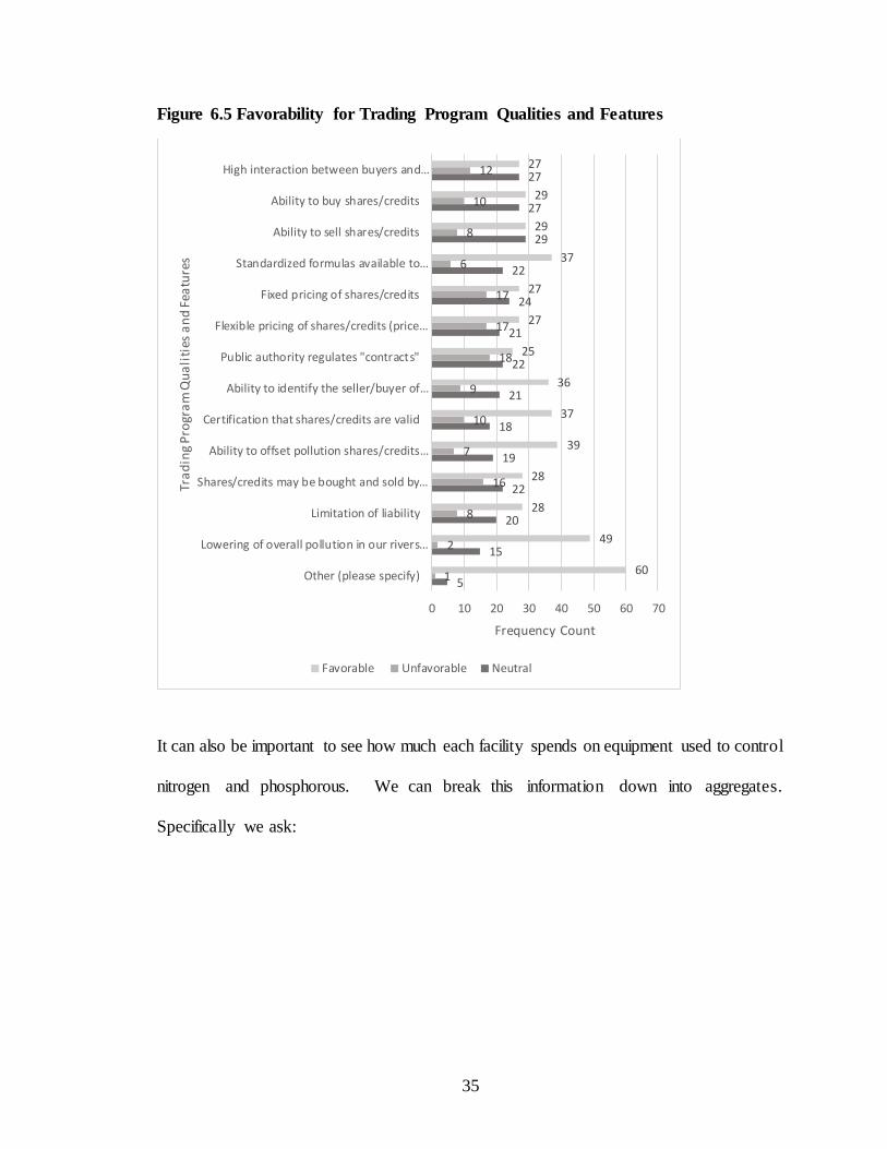
Additionally, we asked respondents how they felt about a variety of qualities and features
for a potential water quality trading market. Popular characteristics can be incorporated,
while less popular qualities can be avoided when possible. Responses for each quality
could be “favorable”, “unfavorable”, or “uncertain”.
21
38
8
0
5
10
15
20
25
30
35
40
Yes No Uncertain
Freq
uen
cy C
ou
nt
Has the Respondent Heard of Water Quality Trading
Page 45
35
Figure 6.5 Favorability for Trading Program Qualities and Features
It can also be important to see how much each facility spends on equipment used to control
nitrogen and phosphorous. We can break this information down into aggregates.
Specifically we ask:
5
15
20
22
19
18
21
22
21
24
22
29
27
27
1
2
8
16
7
10
9
18
17
17
6
8
10
12
60
49
28
28
39
37
36
25
27
27
37
29
29
27
0 10 20 30 40 50 60 70
Other (please specify)
Lowering of overall pollution in our rivers…
Limitation of liability
Shares/credits may be bought and sold by…
Ability to offset pollution shares/credits…
Certification that shares/credits are valid
Ability to identify the seller/buyer of…
Public authority regulates "contracts"
Flexible pricing of shares/credits (price…
Fixed pricing of shares/credits
Standardized formulas available to…
Ability to sell shares/credits
Ability to buy shares/credits
High interaction between buyers and…
Frequency Count
Tra
din
g P
rogr
am
Qu
ali
ties
an
d F
eatu
res
Favorable Unfavorable Neutral
Page 46
36
Based on your best knowledge, please indicate your facility’s expenses for equipment used
mostly to control nitrogen and phosphorous averaged over the past five, ten, and twenty
years.
Figure 6.6 Expense Breakdown (Survey Question)
Average Annual
Expense in Past Five Years
Average Annual
Expense in Past Ten Years
Average Annual
Expense in Past Twenty Years
Under $5,000
$5,000 - $10,000
$10,000 - $50,000
$50,000 - $100,000
$100,000 - $200,000
$200,000 - $500,000
$500,000 - $1M
$1M - $1.5M
$1.5M - $2M
Over $2M
For each of the cost you specified, please give the
percentage of distribution over different methods:
____% biological method
____% chemical method ____%
mechanical method
____% biological method
____% chemical method ____%
mechanical method
____% biological method
____% chemical method ____%
mechanical method
Other types of costs (please specify):
The majority of respondents who reported on this question report spending less than $5,000
on average over the past 5, 10, and 20 years, while some responses exceeded $2,000,000.
Unfortunately, this question went largely unanswered, with the highest number of
responses being 16, for the average annual expense over the past five years. We attempt
Page 47
37
to get the percentage breakdown of where these costs were distributed, i.e. was the cost
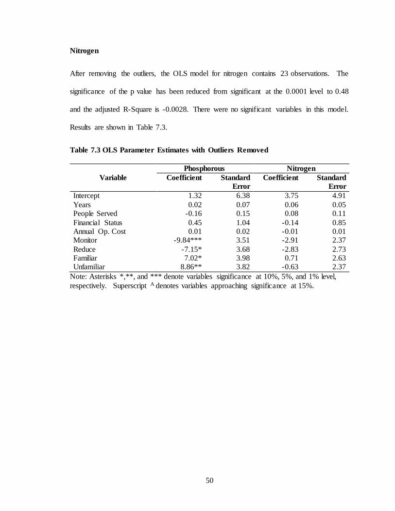
due to biological methods, chemical methods, or mechanical methods? Responses to these
questions were spotty at best.
Finally, we can review the ranked preferences among a list of potential water quality
trading mechanisms. After being provided with a list of descriptions for each market
mechanism, respondents were asked to rank their preferences in the following question:
I would rank these market options as (1 being the most preferred; 2 is less preferred to 1,
and so on):
_____ Seller/Buyer Negotiation
_____ Government Facilitation
_____ Market Exchange
_____ Sole-Source Offset
This question will be covered later in more detail. For now, we can review the responses.
Each mechanism receives its own rank by each respondent. For Seller/Buyer Negotiation,
25 said they prefer this option most, 17 said they prefer it second most, 11 ranked it third,
and 5 ranked it least preferred. For Market Exchange, 7 ranked this item as their most
preferred, 16 ranked it as second most preferred, 14 ranked it third most preferred, and 19
ranked it least preferred, while one respondent ranked this mechanism with a 10. For
Government Facilitation, 13 ranked this as most preferred, 10 ranked it second most
preferred, 14 ranked it third, and 20 ranked it as their least preferred mechanism. Sole-
Source offset received 13 responses for most preferred, 17 responses for second most
preferred, 15 responses for third most preferred, and 11 responses for least preferred, with
one response with a value of 10.
Page 48
38
Figure 6.7 Ranking: Seller/Buyer
Negotiation
Figure 6.8 Ranking: Government
Facilitation
Figure 6.9 Ranking: Market Exchange
Figure 6.10 Ranking: Sole-Source
Offset
25
1711
5
0
10
20
30
1 2 3 4
Freq
uen
cy C
ou
nts
Ranking
Seller/Buyer Negotiation
1310
1420
0
10
20
30
1 2 3 4
Freq
uen
cy C
ou
nts
Ranking
Government Facilitation
7
1614
19
1
0
5
10
15
20
1 2 3 4 10
Freq
uen
cy C
ou
nts
Ranking
Market Exchange
1317
1511
1
0
5
10
15
20
1 2 3 4 10
Freq
uen
cy C
ou
nts
Ranking
Sole-Source Offset
Page 49
39
CHAPTER 7: WILLINGNESS TO PAY FOR ABATEMENT CREDITS
In this chapter, we will discuss the willingness to pay for phosphorous and nitrogen
abatement credits for a potential water quality trading market. The question is presented
in the survey as follows:
Regardless of the characteristics you preferred above, what is the maximum amount your
facility is willing to pay for these shares/credits? We understand that often times the
facilities do not decide these amounts themselves. However, we would like you to specify
the amounts based on your best guess or if you were to make the decision.
To reduce one “unit”; i.e., 1 mg in Total Nitrogen in discharge, the maximum your facility
will be willing to pay per year is:
Figure 7.1 Willingness to Pay: Nitrogen (Survey Question)
$0 $5 $10
$1 $6 $11
$2 $7 $12
$3 $8 $13
$4 $9 $__________
Page 50
40
To reduce one “unit”; i.e., 1 mg in Total Phosphorous in discharge, the maximum your
facility will be willing to pay per year is:
Figure 7.2 Willingness to Pay: Phosphorous (Survey Question)
$0 $5 $10
$1 $6 $11
$2 $7 $12
$3 $8 $13
$4 $9 $__________
The respondent has the option of selecting any of the available boxes with values ranging
from $0-13 or alternatively, the respondent can include an alternative response, if there is
a more appropriate dollar amount. The range of possible responses was generated during
the discussion with a focus group. This question focuses on abatement on a per-unit basis.
Given publicly available information, the total quantity of abatement can be derived for
each facility. In order to analyze the response for the two willingness-to-pay questions, we
will first consider the type of dependent variable, which first appears to be continuous.
Because the respondent can select any dollar amount they see fit, we first begin by
implementing an Ordinary Least Squares model. However, we immediately notice that a
large portion of the respondents reported they would be willing to pay $0. Respondents
were limited to only recording positive dollar value responses, and thus we have
unintentionally censored their possible responses. Therefore, we move beyond OLS and
use a tobit model, which is a common model for censored regression analysis.
Additionally, a quick look at the responses shows significant outliers. Specifically, while
the majority of responses are single or double digit dollar amounts, we have some responses
Page 51
41
that reach as high as $200,000 and $400,000 for willingness to pay responses. Rather than
choosing to keep or discard the outliers, analysis is conducted using OLS and tobit, first
where the outliers are present and second where outliers are removed. To define outliers,
we simply remove observations that are more than 1.5 times the inner quartile range above
the third quartile. Additionally, tests for multicollinearity were conducted. A general rule
of thumb is to further investigate variables when the variance inflation factor (VIF) is
greater than 10. For our data, the highest VIF values were 3.8 (nitrogen model, all
observations present), 3.7 (phosphorous model, all observations present), 2.4 (nitrogen
model, outliers removed), and 2.5 (phosphorous model, outliers removed). Because there
were no values indicating multicollinearity, we can move forward with our analysis.
For all models used in this section, the dependent variables are regressed against the
following explanatory variables from the survey:
Page 52
42
Table 7.1 Explanatory Variables
Explanatory Variable Description
Years The number of years the current facility has been in operation.
People Served The number of households or people the
facility serves.
Financial Status The current financial status of the facility compared to the previous year. Responses
range from 1-7, where 1 is much worse, 4 is about the same, and 7 is much better.
Operating Cost The average annual operating cost of the water quality treatment equipment
currently used in the facility (including labor, electricity/fuel, and materials, but
excluding building costs, installation, and equipment depreciation.
Monitor If the facility is required to monitor
phosphorous, then the response is coded as ‘1’.
Reduce If the facility is required to reduce phosphorous, then the response is coded
as ‘1’.
Familiar If the respondent has heard of water quality trading, then the response is coded
as ‘1’.
Unfamiliar If the respondent has not heard of water quality trading, the response is coded as ‘1’.
Note: Monitor and Reduce are both coded against “Neither”. Familiar and Unfamiliar are both coded against “Not Certain”.
Page 53
43
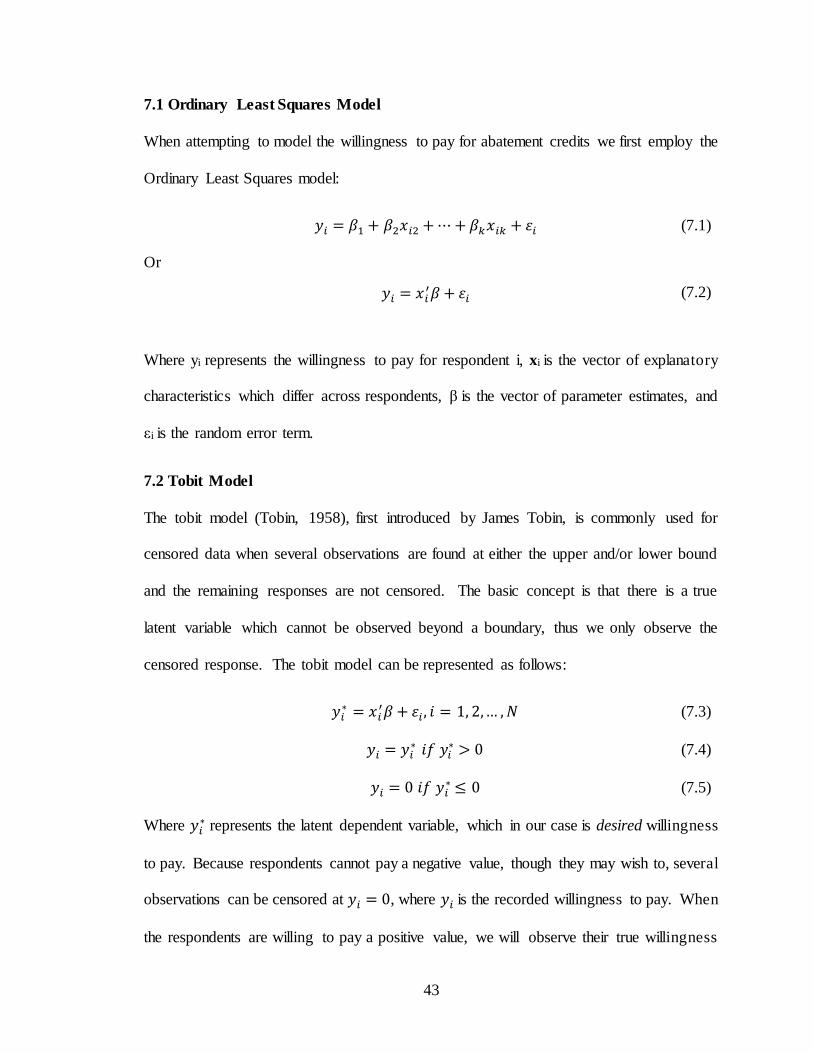
7.1 Ordinary Least Squares Model
When attempting to model the willingness to pay for abatement credits we first employ the
Ordinary Least Squares model:
𝑦𝑖 = 𝛽1 + 𝛽2𝑥𝑖2 + ⋯ + 𝛽𝑘𝑥𝑖𝑘 + 휀𝑖 (7.1)
Or
𝑦𝑖 = 𝑥𝑖′𝛽 + 휀𝑖 (7.2)
Where yi represents the willingness to pay for respondent i, xi is the vector of explanatory
characteristics which differ across respondents, β is the vector of parameter estimates, and
εi is the random error term.
7.2 Tobit Model
The tobit model (Tobin, 1958), first introduced by James Tobin, is commonly used for
censored data when several observations are found at either the upper and/or lower bound
and the remaining responses are not censored. The basic concept is that there is a true
latent variable which cannot be observed beyond a boundary, thus we only observe the
censored response. The tobit model can be represented as follows:
𝑦𝑖∗ = 𝑥𝑖
′𝛽 + 휀𝑖 , 𝑖 = 1, 2,… , 𝑁 (7.3)
𝑦𝑖 = 𝑦𝑖∗ 𝑖𝑓 𝑦𝑖
∗ > 0 (7.4)
𝑦𝑖 = 0 𝑖𝑓 𝑦𝑖∗ ≤ 0 (7.5)
Where 𝑦𝑖∗ represents the latent dependent variable, which in our case is desired willingness
to pay. Because respondents cannot pay a negative value, though they may wish to, several
observations can be censored at 𝑦𝑖 = 0, where 𝑦𝑖 is the recorded willingness to pay. When
the respondents are willing to pay a positive value, we will observe their true willingness
Page 54
44
to pay. The censored regression model describes both the probability of a censorship and
the conditional expected value given a positive response. The probability of 𝑦𝑖 = 0 can
be shown as:
𝑃{𝑦𝑖∗ ≤ 0} (7.6)
= 𝑃{휀𝑖 ≤ −𝑥𝑖′𝛽} (7.7)
= 𝑃 {
휀𝑖
𝜎≤ −
𝑥𝑖′𝛽
𝜎}
(7.8)
= 𝛷 (−
𝑥𝑖′𝛽
𝜎)
(7.9)
= 1 − 𝛷 (
𝑥𝑖′𝛽
𝜎)
(7.10)
And the conditional expected value of 𝑦𝑖 given 𝑦𝑖 > 0 can be shown as:
𝐸{𝑦𝑖|𝑦𝑖 > 0} = 𝑥𝑖′𝛽 + 𝐸{휀𝑖|휀𝑖 > −𝑥𝑖
′𝛽} (7.11)
= 𝑥𝑖′𝛽 + 𝜎
𝜙(𝑥𝑖
′𝛽𝜎 )
𝛷(𝑥𝑖
′𝛽𝜎 )
(7.12)
7.3 Empirical Results: Willingness to Pay for Abatement Credits
In this section, we will review the results obtained using Ordinary Least Squares and a
censored regression model, i.e. the Tobit Model. The reason we will be implementing both
models is due to the fact that while the dependent variable(s) is/are continuous in nature,
there is a clustering of observations at zero. When clustering occurs at the extreme end of
possible responses, that is an indication of censoring, and thus OLS will no longer be the
appropriate model to use. Additionally, we will take note of the presence of extreme
outliers in our dependent variables which can potentially skew our parameter estimates.
Page 55
45
For that reason, we will look at our results with all observations present, and again with
outliers removed for comparison.
Acknowledging the Presence of Outliers
Prior to reviewing the models implemented, we will first address the presence of outliers.
It is important to note that while an observation may be deemed an outlier, it does not mean
the observation is inaccurate. However, due to the scale of our responses, they should also
not be overlooked. There were 81 surveys partially completed. Of the 81 surveys
submitted, there were only 38 responses for willingness to pay for phosphorous and only
36 responses for willingness to pay for nitrogen. We then cleaned the data and created two
new sets. These two new sets would not have any missing values, which is necessary for
some of the Tobit coding to be done later. One set is for phosphorous and contains 29
observations. The other set is for nitrogen and contains 26 observations. Using a simple
formula to calculate outliers from these two sets, we consider any observation which lies a
distance greater than 1.5 times the inner quartile range above Q3 or below Q1 to be a
potential outlier. For phosphorous, we found six outliers ranging from $75 to $400,000.
For Nitrogen, we found three outliers ranging from $750 to $200,000.
7.3.A Reporting OLS Results: All Observations Included
Phosphorous
There were 29 observations used for this model. The overall p value was significant at the
.0001 level which means we have significant evidence that at least one of the coefficients
in our model is not equal to zero, meaning at least one variable is ‘useful’, i.e. that variable
significantly captures a portion of the variance within the model. The adjusted R-Square
was 0.83 which means 83% of the variance among the dependent variables can be
Page 56
46
explained by the model. However, with the presence of extreme outliers, the R-Square
value provided can be misleading. Eight parameter coefficients were estimated in addition
to the intercept. Of the parameter estimates, People Served was significant at the 10% level
while Financial Status and the dummy variable Unfamiliar were approaching significance
at the 15% level. No other variable was significant. It is important to note that while the
overall fit of the model seems rather strong, one outlier in particular has a Cook’s D value
greater than 15, which is considered to be a high amount of leverage. Results can be found
in Table 7.2.
Nitrogen
There were 26 observations used for this model. The overall p value was significant at the
.0001 level and the adjusted R-Square was again 0.83. Of the parameter estimates, we find
similar results to those from the phosphorous model. People Served was significant at the
10% level while Financial Status and the dummy variable Unfamilia r were approaching
significance at the 15% level. No other variable was significant. Again, there was an
observation with a Cook’s D value greater than 15. Results can be found in Table 7.2.
Page 57
47
Table 7.2 OLS Parameter Estimates with All Observations Present
Phosphorous Nitrogen
Variable Coefficient Standard
Error
Coefficient Standard
Error
Intercept 13,243 38269 13,386 21836 Years 284.28 358.68 121.83 202.66
People Served 1,627.16* 818.06 804.40* 431.44 Financial Status -9,245.15A 6245.20 -5,963.39A 3566.68
Annual Operating Cost 115.04 103.77 62.24 0.00 Monitor 23,139 19052 12727 10159 Reduce 10,064 22127 1,885.74 12345
Familiar -4,941.81 20550 -3,585.29 11638 Unfamiliar -28,373A 18504 -16,108A 9905.29
Note: Asterisks *,**, and *** denote variables significant at the 10%, 5%, and 1% levels,
respectively. Superscript A denotes variables approaching significance at 15%.
Page 58
48
7.3.B Interpreting OLS Results (Phosphorous Example)
The results for the two willingness to pay models (phosphorous and nitrogen) have nearly
identical interpretations. The primary difference is that of course the respective estimates
from each table correspond to the willingness to pay for their respective dependent
variables. We can walk through the interpretation for the phosphorous results first,
understanding we will have the same basic interpretation for the nitrogen results.
Additionally, the results will have the same interpretation when for the second set of OLS
models, when the outliers have been removed.
For phosphorous, an intercept of 13,243 means that with no additional information, we
would expect WTP for phosphorous credits to be $13,243. For every additional year of
operation, starting from 0 years, we can expect WTP for phosphorous credits to increase
by $284.28. Results for the number of people served has been adjusted by a factor of
1,000. So for every additional 1,000 people served, we expect to see a $1,627 increase in
WTP for phosphorous credits. Financial status was recorded using a likert scale, with
values ranging from 1-7, were 1 represents the facility is doing “much worse” financia l ly
this year, as compared to the previous year, 4 represents the facility is doing “about the
same”, and 7 means the facility is doing “much better”. For every additional point, starting
from 0, we would expect the WTP for phosphorous credits to decrease by $9,245. Annual
operating cost results were adjusted by a factor of 10,000. So for every additional $10,000
of annual operating cost incurred by the facility, we would expect to see an increase of
$115 in WTP for phosphorous credits. Monitor and Reduce are both part of the same
question. Respondents were asked if their facility was required to Monitor, Reduce, or do
Neither, in terms of phosphorous discharge levels. Because respondents were given the
Page 59
49
option of choosing more than one box, both Monitor and Reduce were dummy coded
against Neither, i.e. Neither was set to a value of 0. When the respondent’s facility
monitors for phosphorous, their expected WTP for phosphorous credits increases by
$23,139 compared to a facility that does not monitor or reduce. Additionally, when a
facility reduces phosphorous levels, WTP for phosphorous credits increases by $10,064
compared to a facility that does neither. Familiar and Unfamiliar were also both part of
the same question, where respondents were asked if they had heard of water quality trading
prior to filling out the survey. Respondents had the option of answering “yes”, “no”, or
“uncertain”. When a respondent said “yes”, then we dummy code their response as a ‘1’
for Familiar. Similarly, when they responded “no”, we dummy code their response as ‘1’
for Unfamiliar. Both Familiar and Unfamiliar are coded against Uncertain. When a
response was ‘1’ for Familiar, the expected WTP for phosphorous credits decreases by
$4,941. When the response was ‘1’ for Unfamiliar, the expected WTP decreases by
$28,373.
7.3.C Reporting OLS Results: Outliers Excluded
Phosphorous
After removing the outliers, the OLS model for phosphorous contains 23 observations. The
significance of the p value has been reduced from significant at the 0.0001 level to 0.29
and the adjusted R-Square value has been reduced to 0.12. While the overall fit of the
model has been reduced, the number of significant parameter estimates has increased. We
no longer see significance in People Served, however we now see Monitor is significant at
the 1% level, Unfamiliar is significant at the 5% level, and Reduce and Familiar are both
significant at the 10% level. Results are shown in Table 7.3.
Page 60
50
Nitrogen
After removing the outliers, the OLS model for nitrogen contains 23 observations. The
significance of the p value has been reduced from significant at the 0.0001 level to 0.48
and the adjusted R-Square is -0.0028. There were no significant variables in this model.
Results are shown in Table 7.3.
Table 7.3 OLS Parameter Estimates with Outliers Removed
Phosphorous Nitrogen
Variable Coefficient Standard
Error
Coefficient Standard
Error
Intercept 1.32 6.38 3.75 4.91
Years 0.02 0.07 0.06 0.05 People Served -0.16 0.15 0.08 0.11
Financial Status 0.45 1.04 -0.14 0.85 Annual Op. Cost 0.01 0.02 -0.01 0.01 Monitor -9.84*** 3.51 -2.91 2.37
Reduce -7.15* 3.68 -2.83 2.73 Familiar 7.02* 3.98 0.71 2.63 Unfamiliar 8.86** 3.82 -0.63 2.37
Note: Asterisks *,**, and *** denote variables significance at 10%, 5%, and 1% level,
respectively. Superscript A denotes variables approaching significance at 15%.
Page 61
51
7.3.D Reporting Censored Regression Results: All Observations Included
For the censored regression model, we implemented the QLIM procedure in SAS. There
are multiple ways to perform a censored regression model in SAS. Another popular
approach is to use the LifeReg procedure. According to the knowledge base on the SAS
Support website, the primary difference between the two procedures is that the QLIM
procedure satisfies all four Moore-Penrose conditions while the Lifereg procedure satisfies
only two Moore-Penrose conditions (SAS Institute Inc., n.d.). To lean on the conservative
side, we chose to satisfy all four conditions, hence using Proc QLIM.
Parameter estimation results from the Tobit model can be interpreted similar to those of
the OLS model with a few exceptions. When the expected value is less than or equal to
zero, we would then set our expected value equal to the zero, i.e. the lower bound,
otherwise the interpretation is the same for positive values as it would be for OLS.
Additionally, we must calculate marginal effects for the model, which will be addressed
shortly.
Phosphorous Parameter Estimates (With Interpretation)
There were 29 observations included in the censored regression model for phosphorous
(52 observations were missing). Of those 29 observations, 10 were censored at the lower
bound where respondents said their willingness to pay for phosphorous credits was $0.00.
For this model, all variables with the exception of Years and Annual Operating Cost were
significant at the 1% level. Years and Annual Operating Cost were not significant at all.
Perhaps the most important result is the estimate for _Sigma is significant at the 1% level
which implies tobit has an advantage over OLS.
Page 62
52
The results estimated for the tobit model can be interpreted as follows: The intercept for
the latent, “desired” willingness to pay for phosphorous credits is $55,648 and is significant
at the 1% level. For every additional year of operation, the respondent should be willing
to pay an additional $4.15 per credit, but this number is not significant. For people served,
we can say that for every additional 1,000 people served, desired willingness to pay
increases by $299, but is not significant. When the financial status increases by one point,
from 0, the willingness to pay decreases by $20,410 and is significant at the 1% level. For
every $10,000 of annual operating cost, the willingness to pay should increase by $269 and
is significant at the 1% level. When the facility monitors phosphorous levels, the
willingness to pay decreases by $1159, compared to not monitoring or reducing, and is
significant at the 1% level. Similarly, if the facility reduces phosphorous levels, their
willingness to pay should decrease by $1617 and is significant at the 1% level. When the
representative is familiar with water quality trading, willingness to pay increases by
$18,623 and is significant at the 1% level. Lastly, when the respondent is unfamiliar with
water quality trading, their willingness to pay for credits should decrease by $14,609 and
is significant at the 1% level.
Monitor and reduce are both dummy coded against “neither monitor or reduce”. A
response can be both monitor and reduce, monitor or reduce, or neither. However, while
familiar and unfamiliar were both dummy coded against “uncertain”, regarding prior
knowledge to water quality trading, it does not make sense for respondents to check more
than one box.
When the results from the parameter estimates are applied to an individual respondent,
those values should be interpreted as being applied to the “desired” willingness to pay.
Page 63
53
When the value is less than or equal to zero, we would map their willingness to pay to zero.
Alternatively, if their desired willingness to pay was greater than or equal to zero, we have
no conflict, and can simply take the results without any necessary adjustments, similar to
OLS. However, this is not OLS, so we will need to take additional steps to interpret the
marginal effects of the explanatory variables on the latent dependent variable. The
remaining estimates for willingness to pay for nitrogen credits (with all observations
included), along with the estimates for willingness to pay when outliers have been removed
will be identical to the interpretation of the estimates we just covered. Therefore, I will
only lightly cover the remaining results until we move on to the marginal effects. These
results can be found in Table 7.4.
Nitrogen Parameter Estimates
There were 26 observations included in the censored regression model for nitrogen (55
missing values). Of those 26 observations, 11 were censored at the lower bound. For
this model, all variables were significant at the 1% level with the exception of Years
which was significant at the 10% level and People Served, which was not significant at
all. The value for _Sigma was also significant at the 1% level. Results are located in
Table 7.4.
Page 64
54
Table 7.4 Tobit Model Parameter Estimates with All Observations Included
Phosphorous Nitrogen
Variable Coefficient Standard Error Coefficient Standard Error
Intercept 55,648*** 4.22 28,435*** 2.27
Years 4.15 190.90 184.26* 105.22
People Served 299.00 408.19 111.67 223.16
Financial Status -20,410*** 16.62 -11428*** 8.56
Annual Operating
Cost 268.77*** 55.019 160.14*** 29.60
Monitor -1,158.95*** 3.49 -304.35*** 1.55
Reduce -1,616.60*** 3.44 -19,708*** 1.12
Familiar 18,623*** 1.85 6,072.51*** 1.01
Unfamiliar -14,609*** 3.40 -11,264*** 2.23
_Sigma 33277*** 1.30 16,894*** 0.64
Note: Asterisks *,**, and *** denote variables significant at the 10%, 5%, and 1% levels, respectively. Superscript AA and A denotes variables approaching significance at 20% and
15%, respectively.
7.3.E Reporting Censored Regression Results: Outliers Excluded
Phosphorous Parameter Estimates
With the outliers removed, there were 24 observations in our model for phosphorous. For
this model, there was a reduction in the number of parameters estimated to be significant.
The only variable significant at the 1% level was _Sigma. People Served was approaching
significance at the 15% level and Familiar was approaching significance at the 20% level.
The remaining estimates were not significant. Results are located in Table 7.5.
Nitrogen Parameter Estimates
With outliers removed, there were 23 observations in our model for nitrogen. For this
model, _Sigma was significant at the 1% level. Monitor was significant at the 10% level.
Years and Reduce were both approaching significance at the 20% level. Results are located
in Table 7.5.
Page 65
55
Table 7.5 Tobit Model Parameter Estimates with Outliers Removed
Phosphorous Nitrogen
Variable Coefficient Standard Error Coefficient Standard Error
Intercept 1.35 26.76 3.63 7.12
Years 0.29 0.28 0.10AA 0.07
People Served 0.36AA 0.23 0.05 0.06
Financial Status -0.38 4.55 -0.80 1.30
Annual Operating
Cost -0.06 0.06 -0.01 0.01
Monitor 1.01 10.51 -5.12* 2.69
Reduce 3.39 13.66 -5.73AA 3.68
Familiar -16.45A 12.72 2.40 3.55
Unfamiliar -10.32 12.34 0.93 3.36
_Sigma 17.58*** 3.58 4.48*** 1.01
Note: Asterisks *,**, and *** denote variables significant at the 10%, 5%, and 1% levels, respectively. Superscript AA and A denotes variables approaching significance at 20% and
15%, respectively.
7.3.F Marginal Effects
To fully take advantage of the tobit model, it is important to remember that we are not only
predicting a linear model, but a censored linear regression model. Specifically, we cannot
forget the possibility of a censored response. Therefore, our marginal effects take the
probability of a censorship into account during the estimation process:
𝜕𝐸(𝑦|𝑥)
𝜕𝑥= 𝛽Pr (𝑦∗ > 0|𝑥)
(7.13)
The formula we are estimating is the instantaneous change in the expected value of
willingness to pay for credits, given the current values of the explanatory variables. From
this static condition, if one of the continuous variables changes by one unit, we can expect
to see the product of the parameter estimate multiplied by the probability of the latent
dependent variable being greater than zero. The more certain we are that the latent variable
is not censored, the more closely related the marginal effect will be to the actual parameter
estimate.
Page 66
56
When prompted, SAS provides marginal effects for each explanatory variable, for each
response. However, rather than display the entire output, it is common to use the average
marginal effects. Interpreting the marginal effects works best for continuous variables.
Let’s first look at the results for the average marginal effects on the willingness to pay for
phosphorous credits when all observations are present. The average marginal effect of
years on willingness to pay is 1.98, which means that from a static point, if the facility was
to gain one year of operation, we would expect an average increase of $1.98 on the latent
willingness to pay. Notice how the marginal effect differs from the parameter estimate,
which was $4.15. People served is reported in units of 1,000 people, so when the number
of people served increases by one unit, i.e. 1,000 people, we would expect willingness to
pay to increase by $142.74. Financial status was reported on a likert scale, so we can say
that when the financial status of the facility increases by one point, we would expect the
willingness to pay to decrease by $9,744. Annual operating cost was recorded in units of
$10,000, so when the annual operating cost increases by $10,000, we expect the willingness
to pay to increase by $128. The remaining explanatory variables are dummy variables, and
so it does not make sense to use marginal effects.
Page 67
57
Table 7.6 Average Marginal Effects for Tobit Model: Outliers Present
Phosphorous Nitrogen
Variable Mean Standard Dev Mean Standard Dev
Years 1.9822193 1.3319205 78.6689957 61.1277921 People Served 142.7436669 95.9143208 47.6745083 37.0442943 Financial
Status -9743.99 6547.32 -4879.00 3791.11
Annual
Operating Cost
128.3164736 86.2201994 68.3709700 53.1259667
Monitor -553.2922078 371.7758376 -129.9398014 100.9665002
Reduce -771.7776056 518.5836014 -8414.09 6537.96 Familiar 8890.54 5973.85 2592.60 2014.51
Unfamiliar -6974.27 4686.25 -4809.26 3736.91
Table 7.7 Average Marginal Effects for Tobit Model: Outliers Removed
Phosphorous Nitrogen
Variable Mean Standard Dev Mean Standard Dev
Years 0.1447811 0.0600696 0.0574715 0.0237006
People Served 0.1786577 0.0741249 0.0266973 0.0110097 Financial Status
-0.1921431 0.0797200 -0.4668878 0.1925389
Annual Operating Cost
-0.0318747 0.0132248 -0.0038386 0.0015830
Monitor 0.5046805 0.2093914 -2.9798569 1.2288570 Reduce 1.7025707 0.7063949 -3.3302241 1.3733442 Familiar -8.2592828 3.4267683 1.3943232 0.5750021
Unfamiliar -5.1807266 2.1494783 0.5398613 0.2226323
Page 68
58
CHAPTER 8: PREFERENCES FOR MARKET MECHANISMS
In this chapter, we will discuss the preferences for different types of market trading
mechanisms for a potential water quality trading market, from the perspective of the
representatives from each municipal sewage treatment facility, i.e. from the point source
perspective. In the survey, we defined four trading mechanisms and then asked
respondents to rank their preferences in the following question:
I would rank these market options as (1 being the most preferred; 2 is less preferred to 1,
and so on):
_____ Seller/Buyer Negotiation
_____ Government Facilitation
_____ Market Exchange
_____ Sole-Source Offset
Not only were respondents asked to select their most preferred mechanism, but they were
asked to rank their preferences from most preferred to least preferred. Ranking preferences
gives a greater amount of insight than simply asking for the most preferred choice.
To analyze the ranking of preferences, we will employ the use of a rank-ordered logist ic
regression model (Hausman & Ruud, 1987), also known as the exploded logit (Punj &
Staelin, 1978). We will first introduce the theoretical model, then we will approach the
analysis for these preferences in two distinct stages. The first stage will focus solely on
item differences to determine if there are detectible differences among preferences for
market trading mechanisms. In this stage, we can determine which mechanisms are most
preferred, if any, and it will also serve as a nice introduction to the empirical model we will
Page 69
59
be implementing and how to interpret the results. For the second stage, we will expand our
model to incorporate other information we have collected from the survey responses. In
doing so, we can take the information gained here and use it to predict the probability of a
particular ranking of preferences for a given facility. Additionally, we will be able to see
how particular facility characteristics play a role in determining which trading mechanisms
are most preferred, thus gaining better insight into which type of mechanism might have
the greatest level of success in a given market.
8.1 Rank Ordered Logistic Regression: Theoretical Model
Discrete choice models offer a wide variety of ways to approach analyzing preferences.
When respondents give complete ranks to their preferences, the rank ordered logist ic
regression model, aka the “exploded logit” captures the probability of the entire ranking of
preferences. The exploded logit is derived from the Random Utility Model (Allison &
Christakis, 1994).
Though the actual underlying utility may be a latent, unobservable value, the Random
Utility Model attempts to account for the ranking of utilities in the following form:
Uij = Vij + εij (8.1)
Decomposing the Random Utility Model, Uij represents the unobserved utility for
respondent (i), given choice j, where j is an element of C i, and Ci represents all possible
choices for respondent (i). Vij is the deterministic portion of the model, which will be
represented as xij’β where xij
’ is the vector of explanatory variables for respondent (i),
associated with item j, and β is the vector of parameter coefficients associated with each of
Page 70
60
the explanatory variables. Lastly, εij is the error term, which is distributed iid extreme-
value, and represents the random component of the model. Notice, by construction, the
deterministic portion of the model condenses to a simple scalar and can easily be written
as:
xij’β → µij (8.2)
The deterministic portion of the model will be plugged into a likelihood function.
Regarding the response variables, we should look again at the Random Utility Model:
Vij → xij’β → µij = yi (8.3)
Where yi = (yi1,…, yiJ)’ and yij represents the response, in this case rank, from respondent
(i) given to item j. The possible rankings will be yij =1,…, J where a ranking of 1 is most
preferred and J is least preferred. Similarly, ri = (ri1,…,riJ)’ where rij represents the item
that received rank j by individual (i). We can then see the relationship between the rankings
of items as:
yij = j rij = k (8.4)
Where yij is the response for item j, from respondent (i), and rij is the rank, k, for item j from
respondent (i). We can then state that items most preferred will also give the highest utility,
thus:
𝑈𝑖𝑟𝑖1> 𝑈𝑖𝑟𝑖2
> ⋯ > 𝑈𝑖𝑟𝑖𝐽 (8.5)
At this stage, we have acknowledged all components of the Random Utility Model. The
next step is to estimate the probability of the above sequence of utilities:
Pr [𝑈𝑖𝑟𝑖1> 𝑈𝑖𝑟𝑖2
> ⋯ > 𝑈𝑖𝑟𝑖𝐽] (8.6)
Page 71
61
We can begin by first estimating the probability of only one item being ranked as most
preferred:
Pr [𝑈𝑖𝑟𝑖1] (8.7)
To do so, we can implement McFadden’s conditional logit model (McFadden, 1974):
𝑒𝜇𝑗
∑ 𝑒𝜇𝑘𝐽
𝑘 =1
(8.8)
In the above model, we are simply describing the likelihood of any item, j, being selected
out of the entire list of possible items. The rank ordered logit model extends the conditiona l
logit model to a product of conditional logits, where each additional term in the product
sequentially removes the previously selected item from the denominator. Let δ ijk = 1 if Yik
≥ Yij, and 0 otherwise. This gives us:
𝐿𝑖 = ∏[exp {𝜇𝑖𝑗}
∑ 𝛿𝑖𝑗𝑘exp {𝜇𝑖𝑘}𝐽
𝑘=1
]
𝐽
𝑗 =1
(8.9)
First consider the term δijk, which acts as an on/off switch, indicating which terms to include
in the denominator and which terms to disregard. Next, consider the ambiguity of the
indexing of the terms by the letter j. In this example, we can choose plug any sequentia l
order of the J items and determine the likelihood of that sequence. We could just as easily
replace the term j with rij, and thus implicitly seek out the likelihood of a particular
sequence of ranked preferences. Extending the above equation to a sample size of n
respondents, we have the log likelihood function:
log 𝐿 = ∑ ∑ 𝜇𝑖𝑗
𝐽𝑖
𝑗=1
− ∑ ∑ 𝑙𝑜𝑔
𝐽𝑖
𝑗=1
[∑ 𝛿𝑖𝑗𝑘
𝐽𝑖
𝑘=1
exp (𝜇𝑖𝑘)]
𝑛
𝑖=1
𝑛
𝑖=1
(8.10)
Page 72
62
It should be obvious that the above equation translates to:
log 𝐿 = ∑ ∑ 𝑥𝑖𝑗’𝛽
𝐽𝑖
𝑗=1
− ∑ ∑ 𝑙𝑜𝑔
𝐽𝑖
𝑗 =1
[∑ 𝛿𝑖𝑗𝑘
𝐽𝑖
𝑘=1
exp (𝑥𝑖𝑗’𝛽)]
𝑛
𝑖=1
𝑛
𝑖=1
(8.11)
Where our goal is to estimate the β coefficients that maximize the likelihood observing the
particular sequence of preferences, given the available data from our respondents.
8.2 Empirical Results: Ranked Preferences
8.2.A Stage 1: Item Differences Only
Recall, respondents were asked to rank their preferences with the following question:
I would rank these market options as (1 being the most preferred; 2 is less preferred to 1,
and so on):
_____ Seller/Buyer Negotiation
_____ Government Facilitation
_____ Market Exchange
_____ Sole-Source Offset
We will use the following abbreviations throughout:
Neg = Seller/Buyer Negotiation
Gov = Government Facilitation
Mkt = Market Exchange
SSoff = Sole-Source Offset
Where the responses can be recorded as:
Page 73
63
𝑅𝑒𝑠𝑝𝑜𝑛𝑠𝑒 = (𝑅𝑎𝑛𝑘𝑁𝑒𝑔 , 𝑅𝑎𝑛𝑘𝐺𝑜𝑣 , 𝑅𝑎𝑛𝑘𝑀𝑘𝑡 , 𝑅𝑎𝑛𝑘𝑆𝑆𝑜𝑓𝑓 ) (8.12)
If for example, the respondent preferred Seller/Buyer Negotiations most, Government
Facilitation second most, Market Exchange third, and least preferred Sole-Source Offset,
their response would be:
𝑅𝑒𝑠𝑝𝑜𝑛𝑠𝑒 = (1𝑁𝑒𝑔 , 2𝐺𝑜𝑣 , 3𝑀𝑘𝑡 ,4𝑆𝑆𝑜𝑓𝑓 ) (8.13)
Our first objective in this stage is to determine whether or not there is at least one item that
is ranked differently among the rest with any level of statistical significance. In order to
do so, we implemented the PHREG statement in SAS, which requires a special data loading
process. The process requires each item (Neg, Gov, Mkt, SSoff) to be dummy coded for
each rank (1, 2, 3, 4), and then stratified across respondents. Keeping the loading process
in mind, we have 324 observations read and 230 observations used. Due to the structure
of our model, this can be interpreted as roughly 324/4 = 81 survey responses read and 230/4
= 57.5 observations being used, where the trailing 0.5 is because one respondent only
ranked 1/4 of the mechanisms. The difference between survey responses read and survey
responses used is due to the fact that respondents were not required to fill out responses to
every question.
In order to determine whether or not at least one item is ranked differently from the rest,
we can look to the three tests provided by the PHREG statement for the global null
hypothesis.
𝐻0: 𝐴𝑙𝑙 𝛽 = 0
𝐻𝐴: 𝐴𝑡 𝑙𝑒𝑎𝑠𝑡 𝑜𝑛𝑒 𝛽 ≠ 0
Page 74
64
The three test statistics provided are the Chi-Square values for the Likelihood Ratio Test,
the Score Test, and the Wald Test. When the Chi-Square value is large, we have significant
evidence to reject the null hypothesis, suggesting that at least one beta is not equal to zero.
The results from the global null hypothesis tests can be seen in Table 8.1.
Table 8.1 Testing Global Null Hypothesis: BETA = 0
Test Chi-Square DF Pr > ChiSq
Likelihood Ratio 15.1463 3 0.0017***
Score 15.8162 3 0.0012*** Wald 15.1675 3 0.0017***
Note: Asterisks *,**, and *** denote variables significance at 10%, 5%, and 1% level,
respectively.
As you can see above, the Chi-Square values for all three likelihood tests are significant at
the 1% level, indicating that at least one beta is not equal to zero, meaning that at least one
mechanism appears to be preferred differently from the others.
Our second objective in this stage of the analysis is to review the parameter estimates. Each
of the four trading mechanisms (Neg, Gov, Mkt, SSoff) will have a parameter estimate.
We should note that one of the parameter estimates will be set equal to zero and the results
will be compared against that value. Sole-Source Offset was arbitrarily chosen to be the
omitted mechanism. The parameter estimates for the item differences follow in Table 8.2.
Page 75
65
Table 8.2 Exploded Logit Parameter Estimates: Item Differences
Parameter DF Parameter
Estimate
Standard
Error
Chi-
Square
Pr >
ChiSq
Hazard
Ratio
Neg 1 0.53095 0.2435 4.7539 0.0292** 1.701 Gov 1 -0.24422 0.2365 1.0663 0.3018 0.783
Mkt 1 -0.33527 0.2450 1.8722 0.1712A 0.715 SSoff N/A 0 N/A N/A N/A 1
Note: Asterisks *,**, and *** denote variables significance at 10%, 5%, and 1% level,
respectively. Superscript A denotes variable approaching significance at the 15% level Note: Compared against SSoff
The null hypotheses being tested here are roughly translated to:
1. 𝐻0: 𝑃𝑟𝑒𝑓𝑒𝑟𝑒𝑛𝑐𝑒 𝑓𝑜𝑟 𝑆𝑆𝑜𝑓𝑓 = 𝑃𝑟𝑒𝑓𝑒𝑟𝑒𝑛𝑐𝑒 𝑓𝑜𝑟 𝑁𝑒𝑔
1. 𝐻𝐴: 𝑃𝑟𝑒𝑓𝑒𝑟𝑒𝑛𝑐𝑒 𝑓𝑜𝑟 𝑆𝑆𝑜𝑓𝑓 ≠ 𝑃𝑟𝑒𝑓𝑒𝑟𝑒𝑛𝑐𝑒 𝑓𝑜𝑟 𝑁𝑒𝑔
2. 𝐻0: 𝑃𝑟𝑒𝑓𝑒𝑟𝑒𝑛𝑐𝑒 𝑓𝑜𝑟 𝑆𝑆𝑜𝑓𝑓 = 𝑃𝑟𝑒𝑓𝑒𝑟𝑒𝑛𝑐𝑒 𝑓𝑜𝑟 𝐺𝑜𝑣
2. 𝐻𝐴: 𝑃𝑟𝑒𝑓𝑒𝑟𝑒𝑛𝑐𝑒 𝑓𝑜𝑟 𝑆𝑆𝑜𝑓𝑓 ≠ 𝑃𝑟𝑒𝑓𝑒𝑟𝑒𝑛𝑐𝑒 𝑓𝑜𝑟 𝐺𝑜𝑣
3. 𝐻0: 𝑃𝑟𝑒𝑓𝑒𝑟𝑒𝑛𝑐𝑒 𝑓𝑜𝑟 𝑆𝑆𝑜𝑓𝑓 = 𝑃𝑟𝑒𝑓𝑒𝑟𝑒𝑛𝑐𝑒 𝑓𝑜𝑟 𝑀𝑘𝑡
3. 𝐻𝐴: 𝑃𝑟𝑒𝑓𝑒𝑟𝑒𝑛𝑐𝑒 𝑓𝑜𝑟 𝑆𝑆𝑜𝑓𝑓 ≠ 𝑃𝑟𝑒𝑓𝑒𝑟𝑒𝑛𝑐𝑒 𝑓𝑜𝑟 𝑀𝑘𝑡
The standard output provided in the Table 8.2 above shows the parameter estimates for
Neg, Gov, and Mkt. SSoff was included in addition to the typical results simply for
comparison, and as you can see was set to zero.
We can see that Neg is significant at the 5% level, meaning there is significant evidence to
suggest there is a difference in preference between Neg as compared with SSoff. Gov does
not appear to be significant, thus we do not have significant evidence to suggest a difference
in preference between Gov and SSoff. The parameter for Mkt is not significant, but it is
approaching significance, meaning there is not quite enough evidence to suggest a
difference in preference between Mkt and SSoff.
Page 76
66
Next we can turn our attention to the Hazard Ratios, which can be interpreted as the odds
of preferring that mechanism to SSoff. Going down the list, Neg is approximately 1.7
times as likely to be preferred compared to SSoff, Gov is 0.78 times as likely to be preferred
compared to SSoff, and Mkt is 0.72 times as likely to be preferred compared to SSoff. The
Hazard Ratio for SSoff is exactly 1, because it is being compared to itself. When simply
looking at the ranking of the preferences, we can look at the value of the parameter
estimates. The larger the value, the greater the preference. We observe:
0.53095𝑁𝑒𝑔 > 0𝑆𝑆𝑜𝑓𝑓 > −0.24422𝐺𝑜𝑣 > −0.33527𝑀𝑘𝑡 (8.14)
Which, as should be expected, matches the mean value for the responses:
1.93𝑁𝑒𝑔 < 2.53𝑆𝑆𝑜𝑓𝑓 < 2.72𝐺𝑜𝑣 < 2.93𝑀𝑘𝑡 (8.15)
These results simply mean on average, Neg is most preferred, SSoff is the second most
preferred, Gov is the third most preferred, and Mkt is the least preferred of these possible
trading mechanisms among our respondents.
We just ranked our preferences and tested for item differences when compared against
SSoff. Next, we can exhaustively test for differences in preference among each pair of
items. The remaining pairs to test will be Neg vs Gov, Neg vs Mkt, and Gov vs Mkt. The
results are in Table 8.3 below:
Table 6.3 Linear Hypothesis Testing
Label Wald Chi-Square DF Pr > ChiSq
Neg vs Gov 9.8388 1 0.0017*** Neg vs Mkt 12.6514 1 0.0004***
Gov vs Mkt 0.1366 1 0.7117
Note: Asterisks *,**, and *** denote variables significance at 10%, 5%, and 1% level, respectively.
Page 77
67
These results show there is a significant difference in preferences between Neg and Gov,
and also a significant difference in preferences among Neg, and Mkt, but there is not a
significant difference in preferences between Gov and Mkt. Pairing this information with
the results from earlier, we can now say:
Seller/Buyer Negotiations are most preferred by respondents. Sole-Source Offset is the
second most preferred mechanism by respondents. The least preferred mechanisms are
Government Facilitation and Market Exchange. Though Government Facilitation is
slightly more preferred than Market Exchange, the difference is not significant, and thus
the order of these trailing preferences could easily be reversed.
Page 78
68
8.2.B Stage 1: Interpret Parameter Estimates (Exploded Logit)
Now that we have reviewed the parameter estimates, we can include them in the exploded
logit model and interpret the results. The primary benefit of using this model is that we
have the ability to take a series of ranked preferences and generate the probability of that
order. We can begin by looking at the structure of the response:
𝑅𝑒𝑠𝑝𝑜𝑛𝑠𝑒 = (𝑅𝑎𝑛𝑘𝑁𝑒𝑔 , 𝑅𝑎𝑛𝑘𝐺𝑜𝑣 , 𝑅𝑎𝑛𝑘𝑀𝑘𝑡 , 𝑅𝑎𝑛𝑘𝑆𝑆𝑜𝑓𝑓 ) (8.16)
By the end, we should be able to determine the probability of a sequence of responses:
𝑅𝑒𝑠𝑝𝑜𝑛𝑠𝑒 = (𝑅𝑎𝑛𝑘𝑁𝑒𝑔 , 𝑅𝑎𝑛𝑘𝐺𝑜𝑣 , 𝑅𝑎𝑛𝑘𝑀𝑘𝑡 , 𝑅𝑎𝑛𝑘𝑆𝑆𝑜𝑓𝑓 ) (8.16)
In the above example, we are seeking the probability of a response where Neg is the most
preferred, Gov is the second most preferred, Mkt is the third most preferred, and SSoff is
the fourth most preferred. We will expand upon this when covariates are introduced in
stage 2.
Recall:
xij’β → µij = βj’x i (8.17)
Because we are simply focusing on item differences without covariates, this model reduces
to:
𝜇𝑗 = 𝛽𝑗 (8.18)
On the following page, we will replace µj, which is the deterministic portion of the random
utility model for item j, with the parameter estimate for item j. We will walk through four
steps. In each step, we will notate the probability we are capturing with a superscript letter.
In the following step, that mechanism will be removed from the pool, and we will continue
the process until we have captured all necessary probabilities.
Page 79
69
Table 8.4 Step 1: 𝐏𝐫𝐨𝐛𝐚𝐛𝐢𝐥𝐢𝐭𝐲 (𝐑𝐞𝐬𝐩𝐨𝐧𝐬𝐞 = (𝟏𝐍𝐞𝐠 ,𝟎𝐆𝐨𝐯 , 𝟎𝐌𝐤𝐭, 𝟎𝐒𝐒𝐨𝐟𝐟 ))
Variable Item j Parameter Estimate
𝑒𝜇𝑗 Hazard Ratio 𝑒𝜇𝑗
∑ 𝑒𝜇𝑘𝐽 =4
𝑘 =1
Neg 1 0.53095 𝑒0.53095 =1.7005 0.40499A
Gov 2 -0.24422 𝑒 −0.24422 = 0.7833 0.18654
Mkt 3 -0.3357 𝑒−0.3357 = 0.7151 0.17031
SSoff 4 0.0000 𝑒0 = 1.0000 0.23816
Sum ∑ 𝑒 𝜇𝑘 = 4.1989𝐽=4
𝑘=1
= 1
Table 8.5 Step 2: 𝐏𝐫𝐨𝐛𝐚𝐛𝐢𝐥𝐢𝐭𝐲 (𝐑𝐞𝐬𝐩𝐨𝐧𝐬𝐞 = (𝟏𝐍𝐞𝐠 , 𝟏𝐆𝐨𝐯 , 𝟎𝐌𝐤𝐭, 𝟎𝐒𝐒𝐨𝐟𝐟 ))
Variable Item j Parameter Estimate
𝑒 𝜇𝑗 Hazard Ratio 𝑒𝜇𝑗
∑ 𝑒𝜇𝑘𝐽=4
𝑘=2
Neg Removed Removed Removed Removed Removed
Gov 2 -0.24422 𝑒 −0.24422 = 0.7833 0.31352B
Mkt 3 -0.3357 𝑒−0.3357 = 0.7151 0.28622
SSoff 4 0.0000 𝑒0 = 1.0000 0.40025
Sum ∑ 𝑒 𝜇𝑘 = 2.4984𝐽=4
𝑘=2
= 1
Table 8.6 Step 3: 𝐏𝐫𝐨𝐛𝐚𝐛𝐢𝐥𝐢𝐭𝐲 (𝐑𝐞𝐬𝐩𝐨𝐧𝐬𝐞 = (𝟏𝐍𝐞𝐠 ,𝟏𝐆𝐨𝐯 , 𝟏𝐌𝐤𝐭, 𝟎𝐒𝐒𝐨𝐟𝐟))
Variable Item j Parameter
Estimate
𝑒 𝜇𝑗 Hazard Ratio 𝑒𝜇𝑗
∑ 𝑒𝜇𝑘𝐽=4
𝑘=3
Neg Removed Removed Removed Removed Removed
Gov Removed Removed Removed Removed Removed
Mkt 3 -0.3357 𝑒−0.3357 = 0.7151 0.41694C
SSoff 4 0.0000 𝑒0 = 1.0000 0.58306
Sum ∑ 𝑒 𝜇𝑘 = 1.7151𝐽=4
𝑘=3
= 1
Table 8.7 Step 4: 𝐏𝐫𝐨𝐛𝐚𝐛𝐢𝐥𝐢𝐭𝐲 (𝐑𝐞𝐬𝐩𝐨𝐧𝐬𝐞 = (𝟏𝐍𝐞𝐠 ,𝟏𝐆𝐨𝐯 , 𝟏𝐌𝐤𝐭, 𝟏𝐒𝐒𝐨𝐟𝐟 ))
Variable Item j Parameter
Estimate
𝑒 𝜇𝑗 Hazard Ratio 𝑒𝜇𝑗
∑ 𝑒𝜇𝑘𝐽=4
𝑘=4
Neg Removed Removed Removed Removed Removed
Gov Removed Removed Removed Removed Removed
Mkt Removed Removed Removed Removed Removed
SSoff 4 0.0000 𝑒0 = 1.0000 1.0000D
Sum ∑ 𝑒 𝜇𝑘 = 1.0000𝐽=4
𝑘=4
= 1
Page 80
70
In the four steps above, rather than simply jumping to the overall probability of a sequence,
we first captured the probability of a particular item being most preferred from all possible
options:
𝑃𝑟𝑜𝑏𝑎𝑏𝑖𝑙𝑖𝑡𝑦 (𝑅𝑒𝑠𝑝𝑜𝑛𝑠𝑒 = (1𝑁𝑒𝑔 , 0𝐺𝑜𝑣 , 0𝑀𝑘𝑡 , 0𝑆𝑆𝑜𝑓𝑓 )) (8.19)
In order to do so, we first take the sum of the available hazard ratios to obtain our sample
space. In the first round, that value was 4.1989. We then take the quotient of the hazard
ratio of the item of interest as it relates to the sum of the hazard ratios, and we then have
the probability of that event occurring. You will notice that for every step, the sum of
probabilities should sum to 1. And with each subsequent step, the previous item has been
removed, thus reducing the sample space within that step. For the fourth and final step in
the probability collection process, you will notice there is only one item, and therefore its
probability of being selected is 1.
To calculate the probability of the rank-order mentioned above:
𝑃𝑟𝑜𝑏𝑎𝑏𝑖𝑙𝑖𝑡𝑦 (𝑅𝑒𝑠𝑝𝑜𝑛𝑠𝑒 = (1𝑁𝑒𝑔 , 2𝐺𝑜𝑣 , 3𝑀𝑘𝑡 , 4𝑆𝑆𝑜𝑓𝑓 )) (8.20)
We can now apply our probabilities to the exploded logit model:
(
𝑒𝜇𝑁𝑒𝑔
∑ 𝑒𝜇𝑘𝐽=4
𝑘 =1
) (𝑒𝜇𝐺𝑜𝑣
∑ 𝑒𝜇𝑘𝐽=4
𝑘 =2
) (𝑒𝜇𝑀𝑘𝑡
∑ 𝑒𝜇𝑘𝐽=4
𝑘=3
) (𝑒𝜇𝑆𝑆𝑜𝑓𝑓
∑ 𝑒𝜇𝑘𝐽=4
𝑘=4
) (8.21)
As mentioned, each probability of interest was notated in order:
(𝐴)(𝐵)(𝐶)(𝐷) → (0.40499)(0.31352)(0.41694)(1.0000) = 0.05294 (8.22)
We can now say that based on our exploded logit model, the probability of a respondent
ranking their preferences as Neg, Gov, Mkt, and lastly SSoff is 0.5294.
Page 81
71
8.2.C Stage 2: Complete Model with Explanatory Variables
In the previous stage, we looked at the rankings of preferences for water quality trading
mechanisms among municipal treatment facility representatives. We then used an
exploded logit model to find the probability of a particular ranking of mechanisms.
Expanding upon that model, we can include explanatory variables. The variables we will
be adding to our model are:
Table 8.8: Explanatory Variables
Explanatory Variable Description
Years The number of years the current facility
has been in operation.
People Served The number of households or people the facility serves.
Financial Status The current financial status of the facility
compared to the previous year. Responses range from 1-7, where 1 is much worse, 4 is about the same, and 7 is much better.
Operating Cost The average annual operating cost of the
water quality treatment equipment currently used in the facility (including
labor, electricity/fuel, and materials, but excluding building costs, installation, and equipment depreciation.
Monitor If the facility is required to monitor phosphorous, then the response is coded as ‘1’.
Reduce If the facility is required to reduce
phosphorous, then the response is coded as ‘1’.
Familiar If the respondent has heard of water
quality trading, then the response is coded as ‘1’.
Unfamiliar If the respondent has not heard of water
quality trading, the response is coded as ‘1’.
Note: Monitor and Reduce are both coded against “Neither”. Familiar and Unfamiliar are both coded against “Not Certain”.
Page 82
72
By including explanatory variables, we can return to the original case where we have the
deterministic portion of the random utility model in the form of:
µij = βj’x i (8.23)
The deterministic portion of the model can be expanded to:
𝜇𝑖𝑗 = 𝛽0𝑗 + 𝛽1𝑗𝑥1𝑖 + 𝛽2𝑗 𝑥2𝑖 + 𝛽3𝑗𝑥3𝑖 + 𝛽4𝑗𝑥4𝑖 + 𝛽5𝑗 𝑥5𝑖 + 𝛽6𝑗 𝑥6𝑖 + 𝛽7𝑗 𝑥7𝑖 + 𝛽8𝑗𝑥8𝑖 (8.24)
Where
𝑗 = 𝑇𝑟𝑎𝑑𝑖𝑛𝑔 𝑀𝑒𝑐ℎ𝑎𝑛𝑖𝑠𝑚 𝑥1 = 𝑦𝑒𝑎𝑟𝑠
𝑥2 = 𝑝𝑒𝑜𝑝𝑙𝑒 𝑠𝑒𝑟𝑣𝑒𝑑 𝑥3 = 𝑓𝑖𝑛𝑎𝑛𝑐𝑖𝑎𝑙 𝑠𝑡𝑎𝑡𝑢𝑠
𝑥4 = 𝑜𝑝𝑒𝑟𝑎𝑡𝑖𝑛𝑔 𝑐𝑜𝑠𝑡 𝑥5 = 𝑚𝑜𝑛𝑖𝑡𝑜𝑟
𝑥6 = 𝑟𝑒𝑑𝑢𝑐𝑒
𝑥7 = 𝑓𝑎𝑚𝑖𝑙𝑖𝑎𝑟 𝑥8 = 𝑢𝑛𝑓𝑎𝑚𝑖𝑙𝑖𝑎𝑟
We should then pay special attention to the individual mechanism being reviewed.
Because our dependent variable is not only the ranking, but also the order in which
mechanisms are ranked, we first look at the individual mechanism. Take note of the
ranking associated with that mechanism by the individual, then we can turn to look at the
explanatory variables paired with the current item being ranked. For this reason, we will
have a series of equations to interpret.
𝜇𝑖𝑁𝑒𝑔 = 𝛽0𝑗 + 𝛽1𝑗 𝑥1𝑖 + 𝛽2𝑗 𝑥2𝑖 + 𝛽3𝑗 𝑥3𝑖 + 𝛽4𝑗𝑥4𝑖 + 𝛽5𝑗𝑥5𝑖 + 𝛽6𝑗 𝑥6𝑖 + 𝛽7𝑗 𝑥7𝑖 + 𝛽8𝑗 𝑥8𝑖 (8.25)
𝜇𝑖𝐺𝑜𝑣 = 𝛽0𝑗 + 𝛽1𝑗𝑥1𝑖 + 𝛽2𝑗 𝑥2𝑖 + 𝛽3𝑗 𝑥3𝑖 + 𝛽4𝑗𝑥4𝑖 + 𝛽5𝑗 𝑥5𝑖 + 𝛽6𝑗 𝑥6𝑖 + 𝛽7𝑗 𝑥7𝑖 + 𝛽8𝑗 𝑥8𝑖 (8.26)
𝜇𝑖𝑀𝑘𝑡 = 𝛽0𝑗 + 𝛽1𝑗 𝑥1𝑖 + 𝛽2𝑗 𝑥2𝑖 + 𝛽3𝑗 𝑥3𝑖 + 𝛽4𝑗𝑥4𝑖 + 𝛽5𝑗 𝑥5𝑖 + 𝛽6𝑗 𝑥6𝑖 + 𝛽7𝑗 𝑥7𝑖 + 𝛽8𝑗 𝑥8𝑖 (8.27)
𝜇𝑖𝑆𝑆𝑜𝑓𝑓 = 𝛽0𝑗 + 𝛽1𝑗𝑥1𝑖 + 𝛽2𝑗 𝑥2𝑖 + 𝛽3𝑗𝑥3𝑖 + 𝛽4𝑗𝑥4𝑖 + 𝛽5𝑗 𝑥5𝑖 + 𝛽6𝑗 𝑥6𝑖 + 𝛽7𝑗 𝑥7𝑖 + 𝛽8𝑗 𝑥8𝑖 (8.28)
Page 83
73
In the equations above, we can see that each line is associated with the deterministic portio n
of the model with respect to a particular mechanism. We can now turn our attention to the
results for the exploded logit model with the explanatory variables included.
Again, we have 324 observations read, however only 152 observations were used. This
can be interpreted as 324/4 = 81 survey respondents and 152/4 = 38 observations used,
indicating a drop from 57.5 down to only 38 observations used. Due to the structure of the
model, observations were only used when respondents completed all questions, hence 19
respondents ranked their preferences, but did not respond to all of the remaining questions,
and so they are dropped from this portion of the analysis when using the PHREG statement.
In order to determine whether or not at least one of the interaction terms was significant,
we can look to the three tests provided by the PHREG statement for the global null
hypothesis.
𝐻0: 𝐴𝑙𝑙 𝛽 = 0
𝐻𝐴: 𝐴𝑡 𝑙𝑒𝑎𝑠𝑡 𝑜𝑛𝑒 𝛽 ≠ 0
The three test statistics provided are the Chi-Square values for the Likelihood Ratio Test,
the Score Test, and the Wald Test. The interpretation is the same as for Stage 1, however,
we have now expanded our model to include explanatory variables. When the Chi-Square
value is large, we have significant evidence to reject the null hypothesis, suggesting that at
least one beta is not equal to zero. The results from the global null hypothesis tests can be
seen in Table 8.9.
Page 84
74
Table 8.9 Global Test for All Beta = 0
Test Chi-Square DF Pr > ChiSq
Likelihood Ratio 32.0438 27 0.2305
Score 31.0140 27 0.2706 Wald 25.2226 27 0.5620
Unlike Stage 1, none of our global tests show significance at the 1% level. However, we
have lost a significant portion of our response variables due to incomplete surveys and we
have also greatly increased the number of explanatory variables. These two factors both
contribute to the loss of significance.
Next, we can look at the parameter estimates for our model. The results that are displayed
below are divided into three sections. Each section corresponds to one of the four trading
mechanisms. The first section represents the parameter estimates for the explanatory
variables when paired with Buyer/Seller Negotiation, the second section represents Market
Exchange, and the third section represents Government Facilitation. Within each section,
the first item is “Mechanism”. Mechanism is essentially an intercept term for the
mechanism within each group. If for example, all explanatory variables were omitted, our
model would reduce back to the same model from Stage 1. However, because we have
now included additional variables, the parameter estimates between Stage 1 and Stage 2
will not be the same. Recall, this model is only an expansion of the model from Stage 1.
Therefore, we are again comparing each variable against its Sole-Source Offset
counterpart. The parameter estimates are provided in the Table 8.10 below.
Page 85
75
Table 8.10 Exploded Logit Parameter Estimates, Complete Model
Parameter DF Parameter
Estimate
Standard
Error
Chi-
Square
Pr >
ChiSq
Hazard
Ratio
Buyer/Seller
Negotiation
Mechanism 1 -0.86954 1.88593 0.2126 0.6448 0.419 Years 1 0.01073 0.01763 0.3702 0.5429 1.011 People Served 1 -0.0000218 0.0000193 1.2732 0.2592 1.000 Financial Status
1 0.19307 0.27073 0.5086 0.4757 1.213
Operating Cost
1 5.63946E-7 3.66571E-7 2.3668 0.1239AA 1.000
Monitor 1 -0.90325 0.91216 0.9806 0.3221 0.405 Reduce 1 -1.58624 1.09837 2.0856 0.1487AA 0.205 Familiar 1 1.08263 1.22527 0.7807 0.3769 2.952 Unfamiliar 1 1.60336 1.26151 1.6154 0.2037A 4.970
Market
Mechanism 1 0.18694 1.91370 0.0095 0.9222 1.206 Years 1 0.00227 0.01736 0.0171 0.8959 1.002 People Served 1 -0.0000541 0.0000319 2.8688 0.0903* 1.000 Financial Status
1 0.17297 0.28947 0.3570 0.5502 1.189
Operating Cost
1 8.80785E-7 4.57215E-7 3.7111 0.0541** 1.000
Monitor 1 -0.75665 0.90299 0.7021 0.4021 0.469 Reduce 1 -2.27761 1.19073 3.6587 0.0558* 0.103 Familiar 1 -0.73877 1.10142 0.4499 0.5024 0.478 Unfamiliar 1 -0.19067 1.08499 0.0309 0.8605 0.826
Government
Facilitation
Mechanism 1 -1.78416 1.87236 0.9080 0.3406 0.168 Years 1 0.00427 0.01729 0.0610 0.8050 1.004 People Served 1 -0.0000329 0.0000256 1.6570 0.1980A 1.000 Financial Status
1 0.12729 0.26362 0.2331 0.6292 1.136
Operating Cost
1 4.68078E-7 3.69692E-7 1.6031 0.2055A 1.000
Monitor 1 0.35065 0.92680 0.1431 0.7052 1.420 Reduce 1 -0.76789 1.12791 0.4635 0.4960 0.464 Familiar 1 0.36017 1.13414 0.1009 0.7508 1.434 Unfamiliar 1 1.31528 1.13675 1.3388 0.2472 3.726
Note: Asterisks *,**, and *** denote variables significance at 10%, 5%, and 1% level, respectively. Superscript A and AA denotes variable approaching significance at the 20% and 15% level, respectively.
Note: Compared against Sole-Source Offset
Page 86
76
In the table of parameter estimates, there are several estimates that stand out. Under
Buyer/Seller Negotiations, the parameter estimates for Operating Cost, Reduce, and
Unfamiliar all appear to be approaching significance. Operating Cost is the most
significant, with a p-value of 0.1239, followed by Reduce with a p-value of 0.1487, and
lastly Unfamiliar with a p-value of 0.2037. Under Market, we observer our most significant
variables. Operating Cost under Market is the single most significant variable from our
results, with a p-value of 0.0541, followed closely by Reduce with a p-value of 0.0558, and
lastly with People Served at 0.0903. The third and final section, Government Facilitat ion,
has two variables approaching significance. Those variables are People Served and
Operating Cost, with respective p-values of 0.1980 and 0.2055.
Before going any further, we should pause to understand what a p-value represents in for
these estimates. Because we are comparing probabilities against Sole-Source Offset, we
can consider a static preference for Sole-Source Offset. We can now consider one of the
variables, for example Operating Cost. Under the Buyer/Seller Negotiation section, when
the Operating Cost increases, does that increase (or decrease) the probability of the
respondents preferring Buyer/Seller Negotiation, as compared to Sole-Source Offset? The
null hypothesis says, “No”. However, when the p-value is small enough, we can say that
we have significant evidence to reject the null hypothesis. In the Operating Cost example,
where we are approaching significance. This means that as Operating Cost increases (or
decreases), there is reason to believe the probability of preferring Buyer/Seller Negotiation
will change. So how much will the probability of preferring Buy/Seller Negotiation
change? If we are to increase the Operating Cost by a single dollar, due to the magnitude
of data, we would see practically no change. Hence the Hazard Ratio is 1.00.
Page 87
77
As there are a variety of explanatory variables, we can shift our attention to one of the
dummy coded variables. If we were to look at Reduce, again for Buyer/Seller Negotiations,
we see an estimate of -1.58624, and when exponentiated, we have a Hazard Ratio of 0.205.
To interpret this type of response, we can say that when a respondent works in a facility
that reduces phosphorous, the odds of the respondent preferring Buyer/Seller Negotiations
to Sole-Source Offset is 0.205 compared to a respondent who works in a facility that is not
required to reduce phosphorous. This is of course only one of several ways to interpret the
results from this type of model.
The resulting parameter estimates have all been in contrast with Sole-Source Offset. We
should also test the explanatory variables individually. The null hypotheses being tested
are:
𝐻0: 𝛽𝑌𝑒𝑎𝑟𝑠,𝑁𝑒𝑔 = 𝛽𝑌𝑒𝑎𝑟𝑠,𝐺𝑜𝑣 = 𝛽𝑌𝑒𝑎𝑟𝑠,𝑀𝑘𝑡 = 0
𝐻𝐴 : = 𝐴𝑡 𝑙𝑒𝑎𝑠𝑡 𝑜𝑛𝑒 𝛽𝑌𝑒𝑎𝑟𝑠,𝑗 ≠ 0
…
𝐻0: 𝛽𝑈𝑛𝑓𝑎𝑚𝑖𝑙𝑖𝑎𝑟 ,𝑁𝑒𝑔 = 𝛽𝑈𝑛𝑓𝑎𝑚𝑖𝑙𝑖𝑎𝑟 ,𝐺𝑜𝑣 = 𝛽𝑈𝑛𝑓𝑎𝑚𝑖𝑙𝑖𝑎𝑟 ,𝑀𝑘𝑡 = 0
𝐻𝐴 : = 𝐴𝑡 𝑙𝑒𝑎𝑠𝑡 𝑜𝑛𝑒 𝛽𝑈𝑛𝑓𝑎𝑚𝑖𝑙𝑖𝑎𝑟,𝑗 ≠ 0
The results from the above hypotheses can be found in Table 8.11 below. Our objective is
to determine if the explanatory variables are distinguishably different among the
mechanisms. For example, when considering the variable Years, can it help us predict the
ranking of Buyer/Seller Negotiations, Government Regulations, or Market Exchange?
While none of the variables appear to be significant, we do see some common trends that
agree with our findings when looking at the parameter estimates. For example, two of the
Page 88
78
most significant parameters were Operating Cost and Reduce, which are also the most
significant here.
Table 8.11 Testing Significance of Explanatory Variables
Label Wald
Chi-Square
DF Pr > ChiSq
Years 0.3980 3 0.9407
People Served 3.1267 3 0.3725 Financial Status 0.5975 3 0.8970 Operating Cost 4.2536 3 0.2353
Monitor 2.3795 3 0.4975 Reduce 4.2794 3 0.2328
Familiar 2.6244 3 0.4532 Unfamiliar 3.6375 3 0.3034
8.2.D Stage 2: Interpreting Results for the Exploded Logit Model with Explanatory
Variables
Once the parameter estimates have been generated, the interpretation of the exploded logit
model is nearly identical to what was discussed in Stage 1. We can again return to the
deterministic portion of the model:
𝜇𝑖𝑗 = 𝛽0𝑗 + 𝛽1𝑗𝑥1𝑖 + 𝛽2𝑗 𝑥2𝑖 + 𝛽3𝑗𝑥3𝑖 + 𝛽4𝑗𝑥4𝑖 + 𝛽5𝑗 𝑥5𝑖 + 𝛽6𝑗 𝑥6𝑖 + 𝛽7𝑗 𝑥7𝑖 + 𝛽8𝑗𝑥8𝑖 (8.29)
Where we can view all four components as:
𝜇𝑖𝑁𝑒𝑔 = 𝛽0𝑗 + 𝛽1𝑗 𝑥1𝑖 + 𝛽2𝑗 𝑥2𝑖 + 𝛽3𝑗 𝑥3𝑖 + 𝛽4𝑗𝑥4𝑖 + 𝛽5𝑗𝑥5𝑖 + 𝛽6𝑗 𝑥6𝑖 + 𝛽7𝑗 𝑥7𝑖 + 𝛽8𝑗 𝑥8𝑖 (8.30)
𝜇𝑖𝐺𝑜𝑣 = 𝛽0𝑗 + 𝛽1𝑗𝑥1𝑖 + 𝛽2𝑗 𝑥2𝑖 + 𝛽3𝑗 𝑥3𝑖 + 𝛽4𝑗𝑥4𝑖 + 𝛽5𝑗 𝑥5𝑖 + 𝛽6𝑗 𝑥6𝑖 + 𝛽7𝑗 𝑥7𝑖 + 𝛽8𝑗 𝑥8𝑖 (8.31)
𝜇𝑖𝑀𝑘𝑡 = 𝛽0𝑗 + 𝛽1𝑗 𝑥1𝑖 + 𝛽2𝑗 𝑥2𝑖 + 𝛽3𝑗 𝑥3𝑖 + 𝛽4𝑗𝑥4𝑖 + 𝛽5𝑗 𝑥5𝑖 + 𝛽6𝑗 𝑥6𝑖 + 𝛽7𝑗 𝑥7𝑖 + 𝛽8𝑗 𝑥8𝑖 (8.32)
𝜇𝑖𝑆𝑆𝑜𝑓𝑓 = 𝛽0𝑗 + 𝛽1𝑗𝑥1𝑖 + 𝛽2𝑗 𝑥2𝑖 + 𝛽3𝑗𝑥3𝑖 + 𝛽4𝑗𝑥4𝑖 + 𝛽5𝑗 𝑥5𝑖 + 𝛽6𝑗 𝑥6𝑖 + 𝛽7𝑗 𝑥7𝑖 + 𝛽8𝑗 𝑥8𝑖 (8.33)
Page 89
79
The explanatory variables are again:
𝑗 = 𝑇𝑟𝑎𝑑𝑖𝑛𝑔 𝑀𝑒𝑐ℎ𝑎𝑛𝑖𝑠𝑚 𝑥1 = 𝑦𝑒𝑎𝑟𝑠 𝑥2 = 𝑝𝑒𝑜𝑝𝑙𝑒 𝑠𝑒𝑟𝑣𝑒𝑑 𝑥3 = 𝑓𝑖𝑛𝑎𝑛𝑐𝑖𝑎𝑙 𝑠𝑡𝑎𝑡𝑢𝑠 𝑥4 = 𝑜𝑝𝑒𝑟𝑎𝑡𝑖𝑛𝑔 𝑐𝑜𝑠𝑡 𝑥5 = 𝑚𝑜𝑛𝑖𝑡𝑜𝑟 𝑥6 = 𝑟𝑒𝑑𝑢𝑐𝑒 𝑥7 = 𝑓𝑎𝑚𝑖𝑙𝑖𝑎𝑟 𝑥8 = 𝑢𝑛𝑓𝑎𝑚𝑖𝑙𝑖𝑎𝑟
Perhaps the best way to use and interpret the results from this model is with a hypothet ica l
example. If we were to receive the following input values:
𝑥1 = 𝑦𝑒𝑎𝑟𝑠 = 10 𝑥2 = 𝑝𝑒𝑜𝑝𝑙𝑒 𝑠𝑒𝑟𝑣𝑒𝑑 = 75,000
𝑥3 = 𝑓𝑖𝑛𝑎𝑛𝑐𝑖𝑎𝑙 𝑠𝑡𝑎𝑡𝑢𝑠 = 6
𝑥4 = 𝑜𝑝𝑒𝑟𝑎𝑡𝑖𝑛𝑔 𝑐𝑜𝑠𝑡 = 500,000
𝑥5 = 𝑚𝑜𝑛𝑖𝑡𝑜𝑟 = 1 𝑥6 = 𝑟𝑒𝑑𝑢𝑐𝑒 = 1
𝑥7 = 𝑓𝑎𝑚𝑖𝑙𝑖𝑎𝑟 = 1
𝑥8 = 𝑢𝑛𝑓𝑎𝑚𝑖𝑙𝑖𝑎𝑟 = 0
We would simply place these values into the four deterministic equations:
Table 8.12 Exploded Logit Deterministic Equations
𝒙𝒎 Explanatory
Variable
Response 𝜷𝑵𝒆𝒈 𝜷𝑮𝒐𝒗 𝜷𝑴𝒌𝒕
𝑥0 Mechanism 1 -0.86954 0.18694 -1.78416
𝑥1 Years 10 0.01073 0.00227 0.00427
𝑥2 People Served 75,000 -0.0000218 -0.0000541 -0.0000329
𝑥3 Financial Status
6 0.19307 0.17297 0.12729
𝑥4 Operating Cost 500,000 5.63946E-7 8.80785E-7 4.68078E-7
𝑥5 Monitor 1 -0.90325 -0.75665 0.35065
𝑥6 Reduce 1 -1.58624 -2.27761 -0.76789
𝑥7 Familiar 1 1.08263 -0.73877 0.36017 𝑥8 Unfamiliar 0 1.60336 -0.19067 1.31528
𝜇𝑁𝑒𝑔 = 2.3636𝐴 𝜇𝐺𝑜𝑣 = −6.1427𝐵 𝜇𝑀𝑘𝑡 = −4.8584𝐶
Note: Superscript A, B, and C
𝐴: 𝜇𝑁𝑒𝑔 = ∑ 𝑥𝑚′ 𝛽𝑚,𝑁𝑒𝑔
𝐵: 𝜇𝐺𝑜𝑣 = ∑ 𝑥𝑚′ 𝛽𝑚,𝐺𝑜𝑣
𝐶: 𝜇𝑀𝑘𝑡 = ∑ 𝑥𝑚′ 𝛽𝑚 ,𝑀𝑘𝑡
Page 90
80
In the four deterministic equations above, we simply took the parameter estimates and
introduced a hypothetical survey response. Given the values generated above, we can
now return to the original objective of the exploded logit model, which is to estimate the
probability of any rank-order of preferences:
𝑃𝑟𝑜𝑏𝑎𝑏𝑖𝑙𝑖𝑡𝑦 (𝑅𝑒𝑠𝑝𝑜𝑛𝑠𝑒 = (𝑅𝑎𝑛𝑘𝑁𝑒𝑔 , 𝑅𝑎𝑛𝑘𝐺𝑜𝑣 , 𝑅𝑎𝑛𝑘𝑀𝑘𝑡 , 𝑅𝑎𝑛𝑘𝑆𝑆𝑜𝑓𝑓 )) (8.34)
Notice the values from the four equations above are located in the second column from the
left, in Table 8.13 below. Given the set of responses from our example, we can now
interpret the current model for Stage 2 in the same manner as we did in Stage 1.
Table 8.13 𝐁𝐞𝐠𝐢𝐧: 𝐏𝐫𝐨𝐛𝐚𝐛𝐢𝐥𝐢𝐭𝐲(𝐑𝐞𝐬𝐩𝐨𝐧𝐬𝐞 = (𝐑𝐚𝐧𝐤𝐍𝐞𝐠,𝐑𝐚𝐧𝐤𝐆𝐨𝐯 , 𝐑𝐚𝐧𝐤𝐌𝐤𝐭, 𝐑𝐚𝐧𝐤𝐒𝐒𝐨𝐟𝐟))
𝝁𝒋 𝒆𝝁𝒋 𝒆𝝁𝒋
∑ 𝒆𝝁𝒋𝑱=𝟒
𝒌=𝟏
𝜇𝑁𝑒𝑔 = -2.3636 𝑒−2.3636 = 0.9408 0.4823
𝜇𝐺𝑜𝑣 = -6.1427 𝑒−6.1427 = 0.0021 0.0011
𝜇𝑀𝑘𝑡 = -4.8584 𝑒−4.8584 = 0.0078 0.0040
𝜇𝑆𝑆𝑜𝑓𝑓 = 0.0000 𝑒0.0000 = 1.0000 0.5126
Sum ∑ 𝑒𝜇𝑗
𝐽=4
𝑘=1
= 1.9507
= 1
Page 91
81
CHAPTER 9: DISCUSSION
Throughout the course of this thesis, we were first introduced to the concept of the hypoxic
zone in the Northern Gulf of Mexico, which is a phenomenon resulting largely from
excessive nutrients pouring into the Mississippi-Atchafalaya River Basin. The
phenomenon is so catastrophic that organizations and researchers all across the United
States have taken an interest in finding a solution to this problem. Rivers, streams, and
other waterways from several states and regions flow into the Mississippi River,
contributing to nutrient loading in the gulf. Though the problem is quite large, the
Mississippi River/Gulf of Mexico Hypoxia Task Force has devised a plan of action. That
plan led to the recruitment of the University of Kentucky through targeted watershed grants
awarded by the United States Environmental Protection Agency. While the Task Force is
determined to restore the Gulf of Mexico to a non-hypoxic state, the actual implementa t ion
process still remained in question. One of the biggest concerns is how to efficiently and
successfully impose new regulations.
The popularity of water quality trading has been rising, due to its theoretical superiority
over previous methods used. However, theory and empirical evidence do not always agree
with one another, which has historically been the case of water quality trading markets.
For a variety of reasons, these markets have suffered from low-trade volume. Perhaps a
contributing factor to the poor performance of these markets can be linked back to the lack
of communication between those designing the market structure and those who would
actually be participating in the market. For this reason, the goal of this thesis was to shed
new light on the preferences of point source polluters, as this approach had never been
Page 92
82
taken before within the Kentucky River Watershed. Rather than simply provide a price for
abatement credits or implement a market mechanism, we sought to gather the opinions and
preferences of the official representatives from each municipal sewage treatment facility
within the Kentucky River Watershed. Representatives from every facility were given the
opportunity to voice their opinions so that no point source in the region was given
preferential treatment. We then regressed their responses for willingness to pay and
preferences among market mechanisms against a variety of explanatory variables ranging
from facility characteristics to prior knowledge of water quality trading.
In order to explain their responses for willingness to pay, we first used ordinary least
squares, but after quickly realizing the censored responses clustering at $0, we moved on
to use a tobit model to account for the censorship. Upon further inspection, we noticed
significant outlying responses for willingness to pay, that could potentially leverage our
model and highly skew our parameter estimates for the explanatory variables. Because
survey responses were gathered anonymously, we could not go back and contact the
respondents to clarify the reasoning behind their responses, and so it was uncertain as to
whether these responses were accurate or there was simply a misunderstanding while
filling out the surveys. Therefore, we modeled the responses with outliers present and with
outliers removed. Focusing our attention on the tobit model, we found that when all
observations were present, nearly every parameter estimate appeared to be statistica l ly
significant at the 1% level for the phosphorous and nitrogen models. However, looking at
the parameter estimates, we see extremely high values. For example, for willingness to
pay for phosphorous credits, the intercept alone is estimated to be $55,648. Contrast that
number against the market price in the Pilot Water Quality Credit Trading Program for the
Page 93
83
Lower St. Johns River, which was only $68.87/pound (Florida Department of
Environmental Assessment & Restoration, 2010). This difference suggests the outliers did
play a role in inflating our estimates. Now turn to the tobit model where outliers have been
removed and we find an estimated intercept of $1.35. In the model with outliers removed,
significance is lost for all but one explanatory variable. This is to be expected for a model
with less than 30 observations. Of the explanatory variables included in our analysis for
phosphorous, the most significant variable was the number of people served is positive ly
correlated with willingness to pay. The second most significant finding was that
representatives who were already familiar with water quality trading were willing to pay
less for credits. When looking at the responses for nitrogen, we found that representatives
working in facilities that monitored phosphorous levels were willing to pay less for
nitrogen credits. We also found that when facilities reduce phosphorous levels, their
“latent” willingness to pay for nitrogen credits decreases. Lastly, we found that the age of
the facility is positively correlated with the “latent” willingness to pay for nitrogen credits.
When looking at preferences among respondents for different types of market trading
mechanisms, we found the most preferred choice was Seller/Buyer Negotiations, followed
by Sole-Source Offsetting, followed by Government Facilitation, and the least preferred
mechanism was Market Exchange.
Perhaps the program most relevant to this study is the Ohio River Basin Interstate Water
Quality Trading Project. On August 9, 2012, the USDA awarded a conservation innovation
grant to the Electric Power Research Institute (EPRI). The $1 million grant was awarded
to assist in moving the ORV Pilot Water Quality Trading Program forward. The interstate
program includes Indiana, Kentucky, and Ohio. The current pilot phase is scheduled to
Page 94
84
run from 2012 through 2015. While other states have implemented their own programs,
the uniqueness of this program is the inclusion of interstate trading rules, which will allow
for states to follow the same rules and will also allow for credit trading between states. The
interstate trading program provides the same incentives as its single-state predecessors,
being that it will provide flexibility for abating parties to seek more cost-effective means
of abatement than installing on-site controls. However, one of the previous constraints to
the success of former markets was the limitation of participants within a geographic scope.
This program will now broaden that geographic bottleneck. As this project is a pilot, the
program will be measuring the success in a variety of ways. Close attention will be paid
to any obstacles that would hinder a full-scale roll-out. The pilot identifies an ultimate goal
of creating a program that can be completely self-sustaining. In order to build a self-
sustaining program, the program would require the implementation of trading mechanisms
and voluntary participation. For a point source to voluntarily participate, knowing the
preferences of point sources for a market trading mechanism is extremely valuable
information, as it could guide a program towards implementing a program which is most
desired by those who it is intended to be used by.
Page 95
85
APPENDICES
Appendix 1: SAS Codes
Exploded Logit SAS Codes
proc means data = exlog;
run;
/*Appendix A*/
proc phreg nosummary;
model rank = dneg dgov dmkt / ties =
exact;
strata id;
Negotiation_Government: test dneg = dgov;
Negotiation_Market: test dneg = dmkt;
Government_Market: test dgov = dmkt;
run;
/*Interaction Terms*/
data explog; set exlog;
/*mkt*/
mktyrs = dmkt*yrs;
mktppl = dmkt*pplserved;
mktfin = dmkt*finstatus;
mktcost = dmkt*opcost;
mktmon = dmkt*mon;
mktred = dmkt*red;
mktneither = dmkt*neither;
mktfam = dmkt*familiar;
mktunfam = dmkt*unfamiliar;
mktuncertain = dmkt*uncertain;
/*neg*/
negyrs = dneg*yrs;
negppl = dneg*pplserved;
negfin = dneg*finstatus;
negcost = dneg*opcost;
negmon = dneg*mon;
negred = dneg*red;
negneither = dneg*neither;
negfam = dneg*familiar;
negunfam = dneg*unfamiliar;
neguncertain = dneg*uncertain;
/*gov*/
govyrs = dgov*yrs;
govppl = dgov*pplserved;
govfin = dgov*finstatus;
govcost = dgov*opcost;
govmon = dgov*mon;
Page 96
86
govred = dgov*red;
govneither = dgov*neither;
govfam = dgov*familiar;
govunfam = dgov*unfamiliar;
govuncertain = dgov*uncertain;
/*ssoff*/
ssoffyrs = dssoff*yrs;
ssoffppl = dssoff*pplserved;
ssofffin = dssoff*finstatus;
ssoffcost = dssoff*opcost;
ssoffmon = dssoff*mon;
ssoffred = dssoff*red;
ssoffneither = dssoff*neither;
ssofffam = dssoff*familiar;
ssoffunfam = dssoff*unfamiliar;
ssoffuncertain = dssoff*uncertain;
run;
proc means data = explog; run;
/*Appendix C*/
proc phreg data=explog nosummary;
model rank = dneg dmkt dgov
negyrs
negppl
negfin
negcost
negmon
negred
negfam
negunfam
mktyrs
mktppl
mktfin
mktcost
mktmon
mktred
mktfam
mktunfam
govyrs
govppl
govfin
govcost
govmon
govred
govfam
govunfam
;
strata id;
Years: test negyrs, mktyrs, govyrs;
Page 97
87
People_Served:test negppl, mktppl, govppl;
Financial_Status: test negfin, mktfin, govfin;
Operating_Cost: test negcost, mktcost, govcost;
Monitor: test negmon, mktmon, govmon;
Reduce: test negred, mktred, govred;
Familiar: test negfam, mktfam, govfam;
Unfamiliar: test negunfam, mktunfam, govunfam;
run;
Tobit SAS Codes
/*using tobit2*/
proc means data = tobit; run;
/*All Obs: Tobit WTP Phos*/
proc qlim data=tobit;
model wtpp = yrs pplserved finstatus opcost mon red familiar unfamiliar;
endogenous wtpp ~ censored(lb=0);
output out=outtobit residual marginal;
run;
/*All Obs: Average Marginal Effects, WTP Phos*/
proc means data = outtobit;
run;
/*All Obs: Tobit WTP Nit*/
proc qlim data=tobit;
model wtpn = yrs pplserved finstatus opcost mon red familiar unfamiliar;
endogenous wtpn ~ censored(lb=0);
output out=outtobitn residual marginal;
run;
/*All Obs: Average Marginal Effects, WTP Nit*/
proc means data = outtobitn;
run;
proc univariate data = tobit;
var wtpp wtpn;
run;
/*Outliers Removed: WTP P */
proc sql;
create table tobitp as
select wtpp, yrs, pplserved, finstatus, opcost, mon, red, familiar, unfamiliar
from tobit
where wtpp < 100;
run;
quit;
proc print data = tobitP; run;
/*Outliers Removed: WTP N */
proc sql;
create table tobitn as
select wtpn, yrs, pplserved, finstatus, opcost, mon, red, familiar, unfamiliar
from tobit
where wtpn < 100;
run;
Page 98
88
quit;
proc print data = tobitn; run;
/*Outliers Removed: Tobit WTP Phos*/
proc qlim data=tobitp;
model wtpp = yrs pplserved finstatus opcost mon red familiar unfamiliar;
endogenous wtpp ~ censored(lb=0);
output out=outtobitp residual marginal;
run;
/*Outliers Removed: Average Marginal Effects, WTP Phos*/
proc means data = outtobitp;
run;
/*Outliers Removed: Tobit WTP Nit*/
proc qlim data=tobitn;
model wtpn = yrs pplserved finstatus opcost mon red familiar unfamiliar;
endogenous wtpn ~ censored(lb=0);
output out=outtobitnn residual marginal;
run;
/*Outliers Removed: Average Marginal Effects, WTP Nit*/
proc means data = outtobitnn;
run;
Page 99
89
Appendix 2: Survey Instrument
Survey of Nitrogen and Phosphorous Discharge and Abatement in the Kentucky River Watershed
Thank you again for agreeing to take part in this research. We
appreciate your time.
Page 100
90
First, we would like to know some characteristics of your facility.
1. How long has your current facility been in operation?
_______________ years
2. About how many households or people is your facility serving?
_______________ households OR _______________ people
3. Use the scale below to rank your facility’s current financial status compared to last year.
Much Worse About the same Much Better
1 2 3 4 5 6 7
4. What is the average annual operating cost of the water quality treatment equipment currently used in
your facility? This cost includes labor, electricity/fuel, and materials, but excludes building costs,
installation, and equipment depreciation.
$ _______________
5. How much does the water quality treatment equipment that you need to maintain your permit cost at
your facility? Please use the table below for your answer.
Type/Name of equipment Cost of purchasing
equipment (please choose
how it was measured)
Year
purchased
Expected
lifetime of the
equipment
Cost at the time of
purchase
Replacement cost as of
2011
$__________________
Years:
Cost at the time of
purchase
Replacement cost as of
2011
$__________________
Years:
Cost at the time of
purchase
Replacement cost as of
2011
$__________________
Years:
Cost at the time of
purchase
Replacement cost as of
2011
$__________________
Years:
Cost at the time of
purchase
Replacement cost as of
2011
$__________________
Years:
Page 101
91
6. On average, how much total nitrogen and total phosphorous is removed from your facility’s effluent stream per year? If your facility is not regulated for total nitrogen
or phosphorous, please mark the closest substitutes (e.g., ammonia for nitrogen) Total Nitrogen ________________ lbs (or closest substitute __________________)
Total Phosphorous ________________ lbs (or closest substitute __________________)
7. Regarding phosphorous, is your facility required to only monitor or to reduce it from your effluent?
monitor only reduce neither
8. Based on your best knowledge, please indicate your facility’s expenses for equipment
used mostly to control nitrogen and phosphorous averaged over the past five, ten, and twenty years.
Average Annual
Expense in Past Five Years
Average Annual
Expense in Past Ten Years
Average Annual
Expense in Past Twenty Years
Under $5,000
$5,000 - $10,000
$10,000 - $50,000
$50,000 - $100,000
$100,000 - $200,000
$200,000 - $500,000
$500,000 - $1M
$1M - $1.5M
$1.5M - $2M
Over $2M
For each of the cost you specified, please
give the percentage of distribution over different methods:
____% biological method
____% chemical method ____%
mechanical method
____% biological method
____% chemical method ____%
mechanical method
____% biological method
____% chemical method ____%
mechanical method
Other types of costs (please specify):
Page 102
92
Among other tools, water quality trading is one way to improve overall water quality in Kentucky while
reducing the cost of compliance. Have you ever heard about the idea of water quality trading?
Yes No Not certain
Water quality trading is an innovative approach to achieve water quality goals more efficiently.
Trading is based on the fact that sources in a watershed can face very different costs to control the
same pollutant. Trading programs allow facilities facing higher pollution control costs to meet their
regulatory obligations by purchasing environmentally equivalent (or superior) pollution reductions
from another source at lower cost, thus achieving the same water quality improvement at lower overall
cost.
While the most well known version of this kind of trading is the “cap-and-trade” design, there are
several alternate methods of implementing a trading system that have been suggested for trading
pollution shares/credits in water quality.
9. Please indicate the trading program qualities that you (your facility) might find favorable (F),
unfavorable (U), or neutral (N):
Qualities/Features Rating
High interaction between buyers and sellers F U
N
Ability to buy shares/credits F U
N
Ability to sell shares/credits F U
N
Standardized formulas available to calculate shares/credits
F U N
Fixed pricing of shares/credits adjusted annually by a
third party
F U
N
Flexible pricing of shares/credits (price varies with supply and demand)
F U N
Public authority regulates “contracts” F U
N
Ability to identify the seller/buyer of the shares/credits F U
N
Certification that shares/credits are valid F U
N
Ability to offset pollution shares/credits within your facility
F U N
Shares/credits may be bought and sold by anyone
(companies, environmental organizations, farmers)
F U
N
Limitation of liability F U
N
Lowering of overall pollution in our rivers (not your pollution discharges specifically)
F U N
Other (please specify) ___________________________________________
F U N
Page 103
93
You are only 2 pages away from being done!
10. Below are some possible trading market descriptions that can be used as an alternative to be
implemented. Based on the description provided, please rank the trading market description according
to the needs and preferences of your facility (1 being the most preferred; 2 is less preferred to 1, and so
on):
Seller/Buyer Negotiation:
Trades take place between buyers and sellers–not through an exchange where shares/credits may be
purchased and sold. These trades are made through direct buyer/seller negotiations. For example,
consider the market for used cars sold by private parties. Car buyers will choose among a variety of
vehicles, each with unique characteristics . The market typically involves bilateral negotiations so that
buyers can personally inspect the vehicles and parties can bargain over the price. A public authority
could monitor the trades and may set rules to facilitate the trades.
Government Facilitation:
Under this system, facilities needing (wanting) to increase their discharges may purchase extra
shares/credits at a fixed price to accommodate this increase. Shares/credits may be accumulated from
many sellers and managed by a clearinghouse such as a public authority. For example, the state or
some other entity pays for pollution reductions and then sells the shares/credits at a fixed price to
polluters needing to exceed their allowable loads. A clearinghouse differs to a broker in a bilateral
market in that clearinghouses eliminate all contractual or regulatory links between sellers and buyers
so that parties interact only with the intermediary. Shares/credit buyers and sellers need not to know
each other.
Market Exchange:
Shares/credits of pollution are traded in a market space, such as the New York Stock Exchange, where
anyone may buy or sell shares/credits. Buyers and sellers meet in a public forum where prices are
observed and quantities of shares/credits are traded. At any one time, there is a unique market-clearing
price so that any interested parties can enter the market to make purchases or sales at the market price.
Prices and market information are available to everyone and jointly determined by all sellers and
buyers. This structure is similar to a stock market except that the pollution shares/credits not stocks are
being transacted.
Sole-Source Offset:
Shares/credits can be generated and used within your facility. For example, if a facility has multiple
points of pollutant discharge, an increase in one point could be possible by an equivalent decrease at
another nearby site. Trades may be made within a facility or between multiple sites within one
facility/organization as far as all sites are located within one watershed .
I would rank these market options as (1 being the most preferred; 2 is less preferred to 1, and so on):
_____ Seller/Buyer Negotiation
_____ Government Facilitation
_____ Market Exchange
_____ Sole-Source Offset
Page 104
94
11. Regardless of the characteristics you preferred above, what is the maximum amount your facility is willing to pay for these shares/credits? We understand that often times
the facilities do not decide these amounts themselves. However, we would like you to specify the amounts based on your best guess or if you were to make the decision.
To reduce one “unit”; i.e., 1 mg in Total Nitrogen in discharge, the maximum your facility will be willing to pay per year is:
$0 $5 $10
$1 $6 $11
$2 $7 $12
$3 $8 $13
$4 $9 $__________
To reduce one “unit”; i.e., 1 mg in Total Phosphorous in discharge, the maximum your facility will be willing to pay per year is:
$0 $5 $10
$1 $6 $11
$2 $7 $12
$3 $8 $13
$4 $9 $__________
Thank you for participating. We appreciate your time.
Please use the space below to write any comments you may have.
Page 105
95
BIBLIOGRAPHY
40 C.F.R. §130. (1985, January 11). Part 130 - Water Quality Planning and
Management. Retrieved from Electronic Code of Federal Regulations:
http://www.ecfr.gov/cgi-bin/text-
idx?SID=6befc5319637bfff549a9443bb681b36&mc=true&node=pt40.22.130&rg
n=div5
Allison, P. D., & Christakis, N. A. (1994). Logit Models for Sets of Ranked Items .
Sociological Methodology, 199-228.
Art, H. W. (1993). A Dictionary of Ecology and Environmental Science (1st ed.). New
York, New York: Henry Holt and Company.
Clean Water Act. (2002, November 27). Federal Water Pollution Control Act [As
Amended Through P.L. 107-303, November 27, 2002]. 303(d). Retrieved 2015,
from http://www.epw.senate.gov/water.pdf
Coase, R. H. (1960). The Problem of Social Cost. Journal of Law and Economics, 3(1),
1-44.
Committee on Environment and Natural Resources. (2000). Integrated assesment of
hypoxia in the Northern Gulf of Mexico: National Science and Technology
Council.
Dales, J. H. (1968). Land, Water, and Ownership. The Canadian Journal of Economics,
1(4), 797-804.
Dales, J. H. (1968). Land, Water, and Ownership. The Canadian Journal of Economics,
1(4), 791-804.
Florida Department of Environmental Assessment & Restoration. (2010). The Pilot
Water Quality Credit Trading Program for the Lower St. Johns River: A Report to
the Governor and Legislature. Division of Environmental Assessment &
Restoration. Retrieved from
https://www.dep.state.fl.us/water/wqssp/docs/WaterQualityCreditReport-
101410.pdf
Fuhrer, G. J., Gilliom, R. J., Hamilton, P. A., Morace, J. L., Nowell, L. H., Rinella, J. F., .
. . Wentz, D. A. (1999). A Systematic Approach to Understanding Nutrients and
Pesticides--National Water-Quality Priorities and Concerns. U.S. Geological
Survey Circular 1225, 84.
Greenhalgh, S., & Selman, M. (2012). Comparing Water Quality Trading Programs:
What Lessons Are There To Learn? The Journal of Regional Analysis & Policy,
42(2), 104-125.
Page 106
96
Hausman, J. A., & Ruud, P. A. (1987). Specifying and Testing Econometric Models for
Rank-Ordered Data. Journal of Econometrics, 34, 83-104.
Hu, W. (2009). Assessment of a Market-Based Water Quality Trading System for
Kentucky River Watershed.
Hypoxia Research Team at LMUCON. (2015). Research. Retrieved 2015, from Hypoxia
in the Northern Gulf of Mexico:
http://www.gulfhypoxia.net/Research/Shelfwide%20Cruises/
Hypoxia Research Team at LUMCOM. (n.d.). About Hypoxia. Retrieved 2015, from
GulfHypoxia.net: http://www.gulfhypoxia.net/Overview/
Marn, M. V., Roegner, E. V., & Zawada, C. C. (2003). Pricing New Products. The
McKinsey Quarterly, 21-30.
McFadden, D. (1974). Conditional Logit Analysis of Qualitative Choice Behavior. (P.
Zarembka, Ed.) Frontiers in Econometrics, 104-142.
Mississippi River Basin Watershed Nutrient Task Force. (2004). A Science Strategy To
Support Management Decisions Related To Hypoxia In The Northern Gulf Of
Mexico And Excess Nutrients In The Mississippi River Basin. U.S. Geological
Circular 1270.
Mississippi River Basin Watershed Nutrient Task Force. (2010). Hypoxia 101: U.S.
Environmental Protection Agency. Retrieved from http://www2.epa.gov/ms-
htf/hypoxia-101
Mississippi River Gulf of Mexico Watershed Nutrient Task Force. (2008). Gulf Hypoxia
Action Plan 2008. Retrieved 2015, from
http://water.epa.gov/type/watersheds/named/msbasin/upload/2008_8_28_msbasin
_ghap2008_update082608.pdf
Mississippi River Gulf of Mexico Watershed Nutrient Task Force. (2013). Reassessment
2013 Assessing Progress Made Since 2008.
Montgomery, W. D. (1972). Markets in Licenses and Efficient Pollution Control
Programs. Journal of Economic Theory, 395-418.
Mueller, D. K., & Helsel, D. R. (1996). Nutrients in the Nation's Waters--Too Much of a
Good Thing? U.S. Geological Survey Circular 1136, 24.
Nixon, S. W. (1995). Coastal Marine Eutrophication: A Definition, Social Causes, and
Future Concerns. Ophelia, 41, 199-219.
O'Hara, J. K., Walsh, M. J., & Marchetti, P. K. (2012). Establishing a Clearinghouse to
Reduce Impediments to Water Quality Trading. The Journal of Regional Analysis
& Policy, 42(2), 139-150.
Page 107
97
Punj, G. N., & Staelin, R. (1978). The Choice Process for Graduate Business Schools.
Journal of Market Research, 15, 588-598.
Rosen, R. (2015). Oceans: The Gulf of Mexico - Chapter 12. Retrieved November 2015,
from Texas Aquatic Science: http://texasaquaticscience.org/oceans-gulf-of-
mexico-aquatic-science-texas/
SAS Institute Inc. (n.d.). Usage Note 30812: Why do PROC QLIM and PROC LIFEREG
give different standard errors on parameters when estimating the same tobit
model? Retrieved from http://support.sas.com/kb/30/812.html
Shortle, J. S., & Horan, R. D. (2008). The Economics of Water Quality Trading.
International Review of Environmental and Resource Economics, 101-133.
Shortle, J. S., & Horan, R. D. (2008). The Economics of Water Quality Trading.
International Review of Environmental and Resource Economics, 101-133.
Stevenson, L. H., & Wyman, B. (1991). Hypoxia, in Dictionary of Environmental
Science. New York, New York: Facts On File, Inc.
Tobin, J. (1958). Estimation of Relationships for Limited Dependent Variables.
Econometrica, 26(1), 24-36.
United States Census Bureau. (2015, October 14). State & County Quick Facts. Retrieved
2014, from http://quickfacts.census.gov/qfd/states/21000.html
United States Environmental Protection Agency. (2008). Targeted Watershed Grants:
Water Quality Trading Projects. Retrieved from
http://water.epa.gov/type/watersheds/trading/twg_index.cfm
United States Environmental Protection Agency. (2012, March 6). Technically Speaking -
Glossary of Terms. Retrieved from
http://water.epa.gov/learn/resources/glossary.cfm
United States Environmental Protection Agency. (2013, September 11). Water: Total
Maximum Daily Loads (303d). Retrieved 2015, from
http://water.epa.gov/lawsregs/lawsguidance/cwa/tmdl/overviewoftmdl.cfm
United States Environmental Protection Agency. (2014, June 5). Frequently Asked
Questions About Water Quality Trading. Retrieved 2015, from
http://water.epa.gov/type/watersheds/trading/tradingfaq.cfm
United States Environmental Protection Agency. (2014, June 5). Water Quality Trading.
Retrieved from http://water.epa.gov/type/watersheds/trading.cfm
United States Environmental Protection Agency. (2015, June 1). History of the Clean
Water Act. Retrieved 2015, from http://www2.epa.gov/laws-regulations/history-
clean-water-act
Page 108
98
United States Environmental Protection Agency. (2015, September 25). Hypoxia 101.
Retrieved from http://www2.epa.gov/ms-htf/hypoxia-101
United States Geological Survey. (2007). Glossary--Nutrients: U.S. Geological Survey.
Retrieved from http://water.usgs.gov/nawqa/glos.html
United States Geological Survey. (2015, August 4). Index of Definitions. Retrieved from
http://toxics.usgs.gov/definitions/
USGS. (2007). Monitoring Network for Nine Major Subbasins Comprising the
Mississppi-Atchafalaya River Basin. (U.S. Geological Survey) Retrieved 2015,
from toxics.usgs.gov: http://toxics.usgs.gov/pubs/of-2007-
1080/major_sites_net.html
VoB, J.-P. (2007, June). Innovation Processes in Governance: The Development of
'Emissions Trading' as a New Policy Instrument. Science and Public Policy,
34(5), 329-343.
Woodward, R. T., Kaiser, R. A., & Wicks, M. B. (2004). The Structure and Practice of
Water Quality Trading Markets. Journal of the American Water Resources
Association, 38(4), 967-980.
Page 109
99
VITA
ANDREW MCLAUGHLIN
Education Bachelor of Science August, 2011
Major: Agricultural Economics Minor: Business Administration
Graduate Certificate May, 2015 Applied Statistics
Professional Experience
Data Analyst March 2015-Present
Center for Clinical and Translational Science Data Analyst August, 2014-March,
2015 Institute for Pharmaceutical Outcomes and Policy
Research Assistant January 2012-June 2014 Department of Agricultural Economics, University of
Kentucky