Water Supply in Rwanda Use of Photovoltaic Systems for Irrigation Gerard Herrero Batalla Andreu Uriach Parellada Supervisors Hans-Georg Beyer Stein Bergsmark Master Thesis in Renewable Energy University of Agder, 2015 Faculty of Engineering and Science This Master Thesis is carried out as a part of the education at the University of Agder and is therefore approved as a part of this education. However, this does not imply that the University answers for the methods that are used or the conclusions that are drawn.
Transcript
Water Supply in Rwanda Use of Photovoltaic Systems for Irrigation
Gerard Herrero Batalla
Andreu Uriach Parellada
Supervisors
Hans-Georg Beyer
Stein Bergsmark
Master Thesis in Renewable Energy
University of Agder, 2015
Faculty of Engineering and Science
This Master Thesis is carried out as a part of the education at the University of Agder and is
therefore approved as a part of this education. However, this does not imply that the University
answers for the methods that are used or the conclusions that are drawn.
i
Abstract
The current energy situation in the world where most of the energy needed is generated from
non-renewable sources such as fossil fuels is no longer sustainable. During few years, non-
renewable sources have become an interesting solution to provide energy to areas with small
needs of electricity, rather than using non-renewable sources.
Therefore, this project has pursued to implement photovoltaics panels to supply energy in a
rural region in central Africa, contributing to the development of the area and proving that this
technology is viable to pump water for irrigation instead of the conventional electric grid.
A rural area between Kidogo Lake and Rilima town, in Bugesera district of Rwanda, has been
chosen as target. This analysis has focused on typical plantations of the country, being the main
crops banana, cassava and maize, each one with very similar maximum water needs; 71
m3/ha_day, 70 m3/ha_day and 67 m3/ha_day, respectively.
The eastern province of Rwanda is formed by seven districts. A preliminary study was developed
in order to find the target area in terms of weather conditions, high temperature and low
rainfall. Therefore, parameters such as precipitation, solar irradiance and evapotranspiration,
among others, have been crucial for deciding the driest zone. Indeed, the Bugesera district is an
ideal candidate due to the reception of a large amount of solar irradiation, with an annual
average of 5,28 kWh/m2_day.
In order to dimension the photovoltaic and water-pumping system, a preliminary research
including a large amount of background was required to determine the best structure. Indeed,
knowing the water demand, we decided the water should be pumped up into a tank, letting it
irrigate the field via gravitation only. A sample irrigation layout was then designed to ensure that
with a number of pipes, water was conveyed to every plant.
The use of a tank not only for storing water, but also as a source of system’s pressure lead us to
calculate the minimum distance from the ground to the bottom. The height obtained of 2,2
meters provides the necessary pressure to distribute water and irrigate the field.
With the energy needed for the water supply, a photovoltaic pumping system, consisting of a
PV generator, inverter and pump, was selected. Our main findings was that the photovoltaic
system must have a rated power of 1,73 kW in order to guarantee proper functioning. For the
photovoltaic system, six STP290 - 24/Vd solar modules from Suntech were chosen, for the water
pumping system, a B50 Electric Drive from the company BBA Pumps. Moreover, and regarding
the inverter system, model Galvo 1.5-1 from company Fronius with a nominal output power
capacity of 1.500 watts was chosen.
ii
Acknowledgements
This thesis has been submitted at the University of Agder, Norway, as a final assignment for our
master’s degree. The support given in this institution has been key for developing the project.
We would also want to thank Polytechnic University of Catalonia for bringing us the chance to
finish our degree abroad.
We would like to express our gratitude to our supervisors Professor Hans-Georg Beyer and Stein
Bergsmark, University of Agder, for the useful comments, remarks and inspiration throughout
this period. Furthermore, we want to thank Professor Joao Leal for providing valuable
information on the fluid dynamics field. Last but not least, a special mention to Fabien
Habyarimana, Renewable Energy PhD Student at University of Agder, for his knowledge of
Rwanda and his useful guidance.
I, Gerard Herrero want to express my sincere gratitude to all my family, giving special thanks to
my parents, Josep and Rosa, and my sister, Joana, for encouraging me to develop my master
thesis abroad and for their great support throughout all my life. I would also like to thank all my
friends for giving me lots of laughs and for our good friendship. In particular, Artur deserves a
special mention for being always there, both in good and bad moments.
I, Andreu Uriach take this opportunity to express my eternal gratitude to my parents, Raimon
and Mercè, for their unconditional support during all these years and the confidence placed on
me. I could not finish without thanking my sister Judit and my brothers Raimon i Xavier for being
The use of photovoltaic systems has increased in recent years. The concern of conserving our
natural resources by using renewable energies has expanded more nowadays than at perhaps
any other time in human history. Using fossil fuel-based energy sources has been proven to
contribute to global climate change. In addition, they are finite so they will be depleted over
time. Clean energy alternatives like solar energy, collected through photovoltaic systems, can
be of great benefit to our environment.
1.1. Background and Motivation
Earth’s climate is changing in ways that affect our whole environment. A lot of ecosystems are
being damaged every day and these changes cannot be caused only by natural aspects.
Bearing in mind that more than half of the world’s electric power is provided by means of fossil
fuels, it is obvious that human activities are contributing to climate change. On the one hand, by
releasing, every year, billions of tons of CO2 into the atmosphere contributing to “the green-
house effect” together with other heat-trapping gases. Indeed, CO2 emissions might be affecting
in a negative way by melting glaciers, therefore sea-water levels are rising every year. On the
other hand, large amount of gases such as NO2, NO and CO are also released every year harming
animals, plants and causing health problems in humans. Climate changes will continue into the
future unless we do not do something about it.
In an effort to find a solution, some studies have been researching several renewable energy
sources in order to provide to the world’s inhabitants the energy needed. These renewables
include bioenergy, wind, solar, geothermal energy as well as tidal power and hydro power.
However, these renewable systems have also disadvantages.
On the one hand, it is not easy to generate the same amount of electricity produced by fossil
fuel generators than by using renewable systems. This may mean that a reduction of the amount
of energy we use is needed or just more energy facilities have to be built. It also indicates that
the best solution to our energy problems may be to have a balance between different power
sources, such as hybrid systems.
On the other hand, the reliability of supply is also a problem. Renewable energy power source
relies on the weather and it is highly intermittent in nature, meaning that most of them
experience both periodical and seasonal variations, thus being unable to guarantee an
interrupted supply of electricity. Hydro generators need precipitation to maintain the dams
filled, wind turbines need wind to move their blades and solar panels need clear skies and sun
irradiance to collect heat and provide electricity and, obviously, this can be unpredictable.
Moreover, the current cost of renewable energy technology is also high in comparison to
traditional fossil fuel generation because of its large capital cost and initial investment.
2
1.2. Problem Statement
Rwanda is part of a group of countries with almost no access to electricity plus high scarcity of
water in rural areas.
Bugesera district is one of the driest areas within the eastern province of Rwanda. Its
precipitation is the lowest in the country, with values below 900 mm per year, and its average
temperature is high, with values above the 21 °C. The combination of these two factors can lead
to droughts, resulting in poor harvests and famine, make Bugesera a very good candidate district
to perform our study.
Nowadays, the most common way to pump water is by using electricity from the grid. Most of
this grid electricity comes from non-renewable energies as renewables are not fully
implemented. However, it is not always possible to connect the water pumping system with the
nearest electric grid due to the high cost involved with extending the main grid. As a
consequence, renewable energy systems have become a suitable cost solution for supplying
remote areas with electricity.
1.3. Goal and Objectives
The main goal of this thesis is to propose an optimal photovoltaic and water pumping system, in
terms of cost and efficiency, in order to pump water for irrigation instead of using the electricity
directly from the grid, which is not easily available. This aim is achieved by accomplishing the
following objectives:
Analysing parameters such as precipitation and solar irradiation within the seven
districts of the eastern province of Rwanda.
Finding relevant crops in the selected area.
Calculating water requirements for each selected crop and the energy needed.
Proposing a basic irrigation layout.
Studying the potential of photovoltaics and the water pumping systems in the selected
area.
Selecting the photovoltaic system by using RETscreen software database.
Analysing the economic cost and the investment.
Comparing the cost, advantages and disadvantages between the chosen system and the
electric grid system.
3
1.4. Key Assumptions and Limitations
The scope of this study is limited to determine both the optimal photovoltaic system to supply
electricity and the water pumping system that can provide enough water for irrigation. In
addition, an economical comparison between electricity from the renewable system or the grid
system will be performed. This analysis has been done by making the following assumptions.
The source for information on the irradiance conditions, the NASA satellite-derived
meteorology and solar energy data are accurately enough for gauging solar photovoltaic
systems.
The calculated water needs are considered the same throughout the project lifetime.
Solar radiation and other parameters such as precipitation and relative humidity
extracted from NASA data base are also considered the same during the project’s
analysis.
While using the RETscreen software and due to the lack of meteorological stations
within the chosen area, the parameters needed were extracted from Kigali station,
which is the nearest one.
Due to the guarantee of the PV panels is about 20 years, the lifetime of the project has
been set as equal.
The final chosen system has the following limitations.
The photovoltaic and water pumping systems are location specific and will not be
optimal for a different location with others basic parameters’ values.
This study will not be focused on the design of the electric grid.
The water tank does not have an integrated and automatic system controlling the
general valve. Therefore, a farmer or worker with enough knowledge needs to be in
charge of it.
The transport and replacement costs have not been taken into account when calculating
the first investment.
1.5. Requirements
The requirements can be divided into functional and non-functional requirements. A functional
requirement specifies a function that a system must be able to perform meanwhile a non-
functional requirement is a statement of how the system must behave, it is a constraint upon
the systems behaviour [1].
1.5.1. Functional Requirements
Energy Supply
Once the photovoltaic system receives sufficient solar irradiance, it must be capable of supplying
enough energy to the water-pumping system. For that reason, at nights the PV system will be
not working and, throughout the day, it will be switching ON and OFF spontaneously depending
on the intensity of the solar irradiance. Therefore, both the PV and the water-pumping systems
must be able to support this continuous variability.
4
1.5.2. Non-functional Requirements
Lifetime
The reliability of every part comprising the system has to be very high. Not only must a long-life
water supply be guaranteed, but maintenance must be minimized in a country where there is a
lack of specialised labour force. Hence, in order to minimize the indirect costs, it is necessary to
invest a larger amount of money.
Portability
Although this research has been focused on a specific area of Rwanda, it is also possible to place
the designed system into another location. However, this new environment should be as similar
as possible to the first one in terms of solar irradiance and sun hours. Yet, the new system
location should be also near to a water resource in a non-sloped land.
Scalability
The water pumping and the photovoltaic systems have been designed to irrigate one hectare of
land and, in fact, if the irrigation of a larger amount of land was required, some changes in both
systems should be implemented. These changes can be the increase of the power capacity of
both the PV and the water pump and increase the number of water tanks. Duplication of the
basic system can also be used. Certainly, these changes come with a significant cost and,
obviously, the irrigation of a larger amount of land is more expensive.
5
1.6. Thesis Outline
The content of this thesis pursues to find a photovoltaic and water pumping system
economically viable and able to compete against the use of electricity directly from the grid. The
thesis comprises 9 chapters, which are detailed below.
Chapter 2 gives an overview of the Rwanda’s geography which is key factor for understanding
the water need in determined areas of the country. Moreover, a brief explanation of the most
important analysed parameters is developed.
Chapter 3 consists in gathering climate information about each of the provinces in Rwanda and
the following analysis of that stats to obtain the most critical area in terms of irrigation.
Chapter 4 focuses on the selection of the crops that fit best in the area studied. Furthermore, it
describes the water requirements for each crop during the different seasons.
Taking that values into account, Chapter 5 proposes an irrigation layout that provides the
minimum elevation height to ensure water flow is conveyed to every plant in the field.
Chapter 6 explains the main components used in photovoltaic and water pumping systems. It
also details the major characteristics of each of the components, costs, operation and
maintenance. The software used to size the system, RETscreen, is introduced and explained.
Finally, Chapter 7 presents the results and Chapter 8 gives the discussion. Chapter 9 provides
the conclusions and the future scope of the work.
6
Chapter 2. Theoretical Background
The Republic of Rwanda is a state in central and east Africa. It is located a few degrees south of
the Equator, being bordered by the Democratic Republic of the Congo, Uganda, Tanzania and
Burundi. The country is located in the African Great Lakes region, its geography is dominated by
mountains in the west and savannah in the east, with a large number of lakes throughout the
country. Despite being located in the tropical belt, Rwanda experiences a temperate climate as
a result of its high elevation. Hence its temperature and rainfall are more moderate than the
surrounding hot and humid equatorial regions.
2.1. Overview of Rwanda
Rwanda covers an area of 26.338 km2 with an estimated population of 12,1 million,
predominantly young and rural, with a density among the highest in Africa. The present borders
were drawn in 2006 with the aim of decentralizing power and removing associations with the
old system and the genocide. The country is structured with five provinces based primarily on
geography (Figure 2.1). These are Northern Province, Southern Province, Eastern Province,
Western Province, and the Municipality of Kigali in the centre.
Figure 2.1: Administrative map of Rwanda (2009) (Source: http://www.rema.gov.rw/soe/background.php)
7
To understand the actual geo-economic situation of the country, it is important to know the
recent history of Rwanda. In 1899 it became under the control of Germany after being it decided
in the Berlin Conference in 1884. That fact decided the beginning of the colonial era. It kept part
of the German East Africa till the First World War, when Belgium invaded it. In 1961 its
monarchical government was formally abolished by referendum and the first parliamentary
elections were held and became independent in 1962. Fighting between the ethnic groups broke
out repeatedly after independence. Finally, social tensions culminated in the 1994 genocide, in
which an estimated of 500.000 to 1 million people were killed.
Since 1994, the government of Rwanda has been able to maintain overall macro stability by
implementing extensive reforms. Agricultural policy is aimed at improving the production of
subsistence and commercial crops. These reforms have contributed significantly to the country’s
strong growth performance. Still, the economy is based mostly on subsistence agriculture where
coffee and tea are the major cash crops for export. Tourism is a key sector as it is growing fast
and is now the country's leading foreign exchange earner. Rwanda is currently at peace and
today has less corruption than the surrounding countries.
The agricultural sector is very important to the economy of Rwanda as it provides employment
to nearly 90 % of the total labour force. Despite being the main source of income, it currently
contributes less than 40 % of the gross domestic product. Production remains low and
constraints to agricultural growth are severe, resulting in scarcity of rural infrastructure and
depressed prices for the two main export commodities, coffee and tea.
2.2. Poverty Profile
Despite the large growth in Rwanda’s economy over the last decade, it is still among the poorest
countries in the world. According to the United Nation’s Human Development Report (2011),
Rwanda was ranked the 22th in terms of poverty.
Figure 2.2: Poverty evolution in Rwanda (Source: The evolution of poverty in Rwanda from 2000 to 2011. Republic of Rwanda. National Institute of Statistics
of Rwanda)
8
As can be seen in Figure 2.2, in 2011 the level of poverty was almost 45 %, having a large
reduction in the Northern Province. Furthermore, it is important to note the great amount of
extreme poverty in every province, as detailed in the Table 2.1.
Table 2.1: Extreme poverty in Rwanda (2011) (Source: The evolution of poverty in Rwanda from 2000 to 2011. Republic of Rwanda. National Institute of Statistics
of Rwanda)
Province Extreme poverty 2010/11 [%]
Kigali City 7,80
Southern Province 31,10
Western Province 27,40
Northern Province 23,50
Eastern Province 20,80
TOTAL 24,10
2.3. Water Resources
Water is a strategic natural resource for any country’s economic, social and cultural
development. As Rwanda is very dependent on agriculture, it increases the importance of this
resource. The country has a dense hydrological network composed of numerous rivers, streams
and wetlands that drain into lakes and other reservoirs.
Although water resources are abundant, they are unevenly distributed in space, category and
quantities. The western region receives considerably higher amounts of rainfall compared to the
east. During rainfall seasons, runoff generated in the hillsides quickly flows to the valley bottoms,
marshlands, rivers or lakes creating an economic water scarcity owing to inadequate
infrastructure. Thus, hillsides can support limited farming during dry seasons. On the other hand,
the eastern part of the country has low rainfall but its lowlands are scattered by a good network
of surface water bodies with significant flows and stock [2].
9
Figure 2.3: Hydrography (lakes and rivers) (Source: The government of Rwanda, Ministry of Agriculture & Animal Resources. Rwanda Irrigation Master Plan.)
Rwanda is divided into two major drainage basins (Figure 2.3): the Nile to the east covering 67
% and delivering 90 % of the national waters and the Congo to the west, which covers 33 % and
handles all national waters. How are these resources distributed is specified in Table 2.2.
Table 2.2: Water distribution in Rwanda (Source: The government of Rwanda, Ministry of Agriculture & Animal Resources. Rwanda Irrigation Master Plan.)
Water Resources Area [ha] Share of Total
Runoff for small reservoirs 125.627 21,0%
Runoff for dams 31.204 5,2%
Direct river and flood water 80.974 13,6%
Lake water resources 100.153 16,8%
Groundwater resources 36.434 6,1%
Marshlands 222.418 37,3%
10
2.4. Climate Data
The selection of the area depends first and foremost to the particular climate conditions.
Therefore, an exhaustive study of the territory is crucial for obtaining which area is the driest.
Basic climatic conditions and the respective information are taken from reliable sources such as
NASA website, Joint Research Centre and FAO/AGLW concerning the irrigation needs. To assess
the need for irrigation, information on precipitation and evapotranspiration is needed and will
be explained in this chapter.
2.4.1. Temperature
Rwanda is located just south of the equator. Because of its high altitude, its temperature and
rainfall are more moderate than the surrounding hot and humid equatorial regions, despite
having the same annual cycles. The temperature throughout the year is considerably constant,
where the lowest registers are observed in highlands with temperatures ranging between 15
and 17 °C. On the other hand, moderate ones are generally in mid height areas temperatures
can vary between 19 and 21 °C. Finally, in the east and southwest temperatures are higher due
to its low height profile, being able to reach temperatures above 30 °C.
2.4.2. Precipitation
Precipitation is the main source of water for agriculture, as more than 90 % of Rwanda’s
agriculture is rain-fed. However, it is unevenly distributed in time and space, with about half of
precipitation occurring in one quarter of the year (Table 2.3). Rainfall ranges from as low as 700
mm in the Eastern Province to about 2000 mm in the high altitude north and west.
Table 2.3: Temporal distribution of precipitation
Period Season description Share of Total Annual Precipitation [%]
Feb. - May. Long rains (April being the wettest month) 48
June - Mid. Sept.
Long dry spell Very little rains of 25-50 mm (especially
in high altitudes)
Mid. Sept. -Dec.
Short rains (November being the wettest during this period)
30
Dec. - Jan. Short rains with short dry spell 22
11
2.4.3. Effective Precipitation
The effective precipitation is the amount of rainfall added and stored in the soil. When raining,
part of the water percolates below the root zone of the plants and part of the rain water flows
away over the soil surface as run-off. This deep percolation water and run-off cannot be used by
the plants. In other words, part of the rainfall is not effective. The remaining part is stored in the
root zone and can be used by plants. This remaining part is called effective rainfall or
precipitation. The factors which influence which part is effective and which is not, include the
climate, the soil texture, the soil structure and the depth of the root zone [3].
There are several ways to calculate the effective precipitation based on real rainfall. According
to Mr. Habyarimana, F., the most reliable methods to calculate the effective rainfall are by using
a formula given by FAO/AGLW or the Empirical one, both equations extracted from software
CROPWAT 8.0.
The effective precipitation PEFF is given in mm per period of interest and is gained from the
monthly precipitation using the formulas 2.1 and 2.2.
FAO/AGLW formula
𝑃𝐸𝐹𝐹 = 0,6 ∗ 𝑃𝑀𝑂𝑁𝑇𝐻 − 10𝑚𝑚
𝑖𝑓 𝑃𝑀𝑂𝑁𝑇𝐻 ≤ 70 𝑚𝑚 (2.1)
𝑃𝐸𝐹𝐹 = 0,8 ∗ 𝑃𝑀𝑂𝑁𝑇𝐻 − 24𝑚𝑚
𝑖𝑓 𝑃𝑀𝑂𝑁𝑇𝐻 > 70 𝑚𝑚
Empirical formula
𝑃𝐸𝐹𝐹 = 0,5 ∗ 𝑃𝑀𝑂𝑁𝑇𝐻 − 5𝑚𝑚
𝑖𝑓 𝑃𝑀𝑂𝑁𝑇𝐻 ≤ 50 𝑚𝑚 (2.2)
𝑃𝐸𝐹𝐹 = 0,7 ∗ 𝑃𝑀𝑂𝑁𝑇𝐻 + 20𝑚𝑚
𝑖𝑓 𝑃𝑀𝑂𝑁𝑇𝐻 > 50 𝑚𝑚
Where,
PEFF is the effective precipitation (mm)
PMONTH is the monthly precipitation (mm)
By using the real rainfall values, monthly effective precipitation has been calculated with these
two different methods.
12
2.4.4. Evapotranspiration
Evapotranspiration or ET is a term describing the loss of water from the soil into the atmosphere
as vapour from surfaces, including soil evaporation and transpiration from vegetation (Figure
2.4). The water generally enters the plant through the root zone, is used for various bio-
physiological functions including photosynthesis, and then passes back to the atmosphere
through the leaf stomata.
There are several parameters that affect the evapotranspiration values. Temperature, relative
humidity, wind and air movement are some of them.
Temperature: When temperature rises, transpiration increases too, particularly during
the growing season, when the air is warmer due to stronger sunlight and warmer air
masses. Thus, the pores in stems and leaves opens and water is released whereas cold
weathers produce a closure of them.
Relative humidity: the larger the humidity, the more difficult it is for water to evaporate
because the water vapour saturation. Therefore, when the humidity increases the
transpiration decreases and vice versa.
Wind and air movement: Transpiration increases whilst wind blows as the saturated air
surrounding the leaf moves away and is replaced by dried air. In case the wind speed is
low, the air around the leaf may not move enough which would turn into a raise of the
humidity and consequently a decrease of the transpiration.
Figure 2.4: Global rainfall scheme (Source: FAO)
13
2.4.5. Solar Irradiance
Solar irradiance is a measure of how much solar power, in the form of electromagnetic radiation,
a specific land area receives (power per unit area on the earth’s surface). Irradiance is not a
constant value, it is changing throughout the year depending on the seasons. It also varies along
the day depending on the position of the sun and the weather.
As shown in Figure 2.5, not all the solar radiation reaches the earth’s surface. At an average
distance of 150 million kilometres from the Sun, the outer atmosphere of Earth receives
approximately 1367 W/m2 of insolation (World Meteorological Organisation). As solar irradiance
passes through the earth’s atmosphere, some of it is absorbed and scattered by air molecules,
water vapour and clouds. Some of the radiation is reflected straight back out into space
(increasing when sky is full clouds) meanwhile the rest arrives on the Earth’s surface. Once the
radiation arrives at the surface, some of it is immediately reflected back into the sky. This
amount depends on the nature of the actual surface – fresh snow can reflect up to 95 % while
Rwanda is located in East Africa at approximately two degrees below the equator. It is
characterised by Savannah climate and its geographical location and weather conditions provide
enough solar irradiation intensity, approximately equal to 5 kWh/m2_day with a peak of sun
hours of also 5 hours per day.
Figure 2.5: Solar radiation scheme (Source: http://www.everredtronics.com/Solar.Download.html)
14
2.5. Surface Data
2.5.1. Slope
Another important factor is the land’s slope. Due to the crops chosen, banana, cassava and
maize do not require large slopes for their growth and being flat lands more easily to plant, we
decided to find a non-sloped crop land, or at least one with a small tilt.
As it can be seen in Figure 2.6 and focusing in the eastern part of Rwanda, there are several
regions where the slope is appropriate to grow a crop. Most of the eastern province have good
conditions in terms of slopes. Certainly, both the north and the southeast parts of have the best
slope conditions.
Figure 2.6: Rwanda slope percentage (Source: The government of Rwanda, Ministry of Agriculture & Animal Resources. Rwanda Irrigation Master Plan.)
15
Chapter 3. Data Collection, Analysis and Selected Area
The design of photovoltaic systems require the collection of different types of data and a
subsequent analyses in order to find the suitable area to maximize the PV yield. In this chapter
it is explained how the data is analysed and how the studied area is chosen.
All data is obtained from reliable sources. Temperature and precipitation values are extracted
from NASA website, solar irradiance values from Joint Research Centre (The European
Commission’s in-house science service) and evapotranspiration from CROPWAT 8.0 software,
developed by FAO (Food and Agriculture Organization of the United Nations).
3.1. Introduction
In order to find the appropriate area within Rwanda for location of the proposed system, a first
overview of the main parameters (temperature and precipitation) for each province has been
developed to delimit the scope of the analysis. As explained in Theoretical Background, Rwanda
is a country divided by five different regions: the Eastern Province, City of Kigali, Northern
Province, Southern Province and Western Province (Figure 3.1).
Once the scope have been delimited, a second analysis of different parameters throughout the
chosen province has also been developed. As stated before, the parameters evaluated have
been the temperature, the precipitation, the solar irradiance and the surface slope as well as
the water resources.
The suitable target area must not only have a high annual average temperature but also a low
annual average precipitation. In addition, it must receive a large amount of solar irradiance
Figure 3.1: Rwanda province map (Source: http://www.theiguides.org/public-docs/guides/rwanda)
16
during the whole year and should be in a flat area or on gently slope simply to facilitate the task
of planting and irrigating.
Even though Rwanda has many water resources, unfortunately they are not equally distributed.
Rainfall is high in the western part of the country and low in the east. Therefore, farms in the
eastern part are the most vulnerable. However, the eastern part has abundant rivers and lakes
that could be used for irrigation purposes.
3.2. Main Area Selection
3.2.1. Province Selection
In order to find the most suitable province, a first overview of the annual average temperature
and precipitation has been compiled. The following maps of temperature and rainfall (Figure
3.2) have been analysed and, as a result, the best region to place the system proposed is the
eastern province.
As it can be seen in Figure 3.2, the highest annual average temperature is focused in the eastern
part of the country together with the lowest annual average precipitation. That is why all the
subsequent analyses were focused within the eastern province.
Figure 3.2: Annual average temperature and rainfall (Source: The government of Rwanda, Ministry of Agriculture & Animal Resources. Rwanda Irrigation Master Plan.)
17
3.2.2. District Selection
Once the eastern province is chosen, it is necessary to analyse the parameters of each district
within this region. The eastern province is composed by seven districts: Bugesera, Gatsibo,
Kayonza, Kirehe, Ngoma, Nyagatare and Rwamagana.
Within Rwanda there are only four weather stations distributed through the whole country. One
station is located in Kigali, the capital of the country. There is one station in Butare and one more
in Rubona-Colline, both cities in the southeast of Rwanda and the last one is located in
Ruhengeri, a northeast city. As it is observed, there are no weather stations in the eastern part
of the country and that is the reason why some data is the same between several districts.
In order to design both the PV and the water-pumping system with enough capacity to supply
the largest water demand, it is necessary to take the lowest effective precipitation and the
highest crop water need. Consequently, the highest evapotranspiration value.
Temperature
Focusing on the temperature, in Figure 3.3 it is observed a very similar trend for all the districts.
However, it is also observed that both the highest maximum and minimum temperatures
correspond to the district of Bugesera.
25,00
27,00
29,00
31,00
33,00
35,00
37,00
39,00Maximum Temperature Monthly Average TMAX [°C]
BUGESERA
NYAGATARE / KAYONZA /GATSIBO / RWAMAGANA
NGOMA / KIREHE
14,00
14,50
15,00
15,50
16,00
16,50
17,00
17,50
18,00
Minimum Temperature Monthly Average TMIN [°C]
BUGESERA
NYAGATARE / KAYONZA /GATSIBO / RWAMAGANA
NGOMA / KIREHE
Figure 3.3: Maximum and minimum annual temperature trends per district
18
Effective precipitation
As stated in the section 2.3.3, the effective rainfall has been calculated by using two different
methods. Table 3.1 shows the annual effective rainfall average values for each district.
FAO/AGLW formula [mm/month] Effective Precipitation using
Empirical formula [mm/month]
BUGESERA 52,08 76,93
NYAGATARE KAYONZA GATSIBO
RWAMAGANA
58,03 85,27
NGOMA KIREHE
60,01 86,91
As it is shown in Table 3.1, the lowest values appear when using FAO/AGLW formula. Therefore,
in the subsequent analyses, FAO’s formula is chosen due to it is more restrictive than the
Empirical formula.
In addition, it is observed in Figure 3.4 that Bugesera district has the lowest effective
precipitation from March until the end of the year as well as during the rainy season.
Figure 3.4: Annual effective precipitation trend per district
0,00
20,00
40,00
60,00
80,00
100,00
120,00
Effective Precipitation using FAO/AGLW formula [mm/month]
BUGESERA
NYAGATARE / KAYONZA /GATSIBO / RWAMAGANA
NGOMA / KIREHE
19
Evapotranspiration
As mentioned above, it is necessary to find the highest evapotranspiration value in order to
design a system able to supply the highest water need. This ET0 values are provided by CROPWAT
8.0 software and they are shown in Figure 3.5. As can be seen, the ET0 of each district follows a
similar trend as well as the temperature. Nevertheless, the ET0 value for Bugesera is higher from
April until the end of the year, coinciding with the rain season.
Figure 3.5: Annual evapotranspiration trend per district
Solar Irradiation
It is difficult to find out which district has the highest solar irradiation as seen in Figure 3.6
because, as expected, they also have a similar trend throughout the whole year. However,
Bugesera has the highest annual average solar irradiation with 5,28 kWh/m2_day, shown in
Table 3.2.
Figure 3.6: Annual solar irradiation trend per district
3,203,704,204,705,205,706,206,707,20
Evapotranspiration ETo [mm/day]
BUGESERA
NYAGATARE
NGOMA
KIREHE
KAYONZA
GATSIBO
RWAMAGANA
4,10
4,60
5,10
5,60
6,10
Solar Irradiation [kWh/m2_day]
BUGESERA
NYAGATARE
NGOMA
KIREHE
KAYONZA
GATSIBO
RWAMAGANA
20
Table 3.2: Annual average solar irradiation per district
DISTRICT Annual Average Solar Irradiation
[kWh/m2_day]
BUGESERA 5,28
NYAGATARE 5,23
NGOMA 5,23
KIREHE 5,02
KAYONZA 4,98
GATSIBO 5,10
RWAMAGANA 5,08
Table 3.2 above shows the annual average solar irradiation kWh/m2_day per district. It is
observed that irradiation is quite similar but Bugesera is slightly higher than the others.
Chart summary and other information
Table 3.3: Average of the analysed parameters per district
DISTRICT Annual
Irradiation [kWh/m2_day]
Annual Effective Precipitation [mm/month]
Annual ET0 [mm/day]
Annual TMIN [°C]
Annual TMAX [°C]
BUGESERA 5,28 52,08 4,90 16,02 31,57
NYAGATARE 5,23 58,03 4,53 15,81 30,73
NGOMA 5,23 60,01 4,58 15,95 30,69
KIREHE 5,02 60,01 4,53 15,95 30,69
KAYONZA 4,98 58,03 4,49 15,81 30,73
GATSIBO 5,10 58,03 4,51 15,81 30,73
RWAMAGANA 5,08 58,03 4,51 15,81 30,73
Once all the parameters have been discussed and analysed, it is observed (Table 3.3) that all
districts have similar values. However, Bugesera is the one that stands out above the others due
to its low effective precipitation as well as its high minimum and maximum temperatures. In
addition, its annual average evapotranspiration is also the highest.
Poverty is also taken into account for deciding the district. The region of Bugesera, which has
experienced long periods of droughts and low levels of rainfall, is one of the poorest regions in
Rwanda with a percentage of food insecure household between 36 and 40 (Figure 3.7).
21
Bugesera is also one of the poorest districts in the Eastern Province in Rwanda as shown in table
3.4.
Table 3.4: Percentage of poverty in Eastern province (Source: Economic Development and Poverty Reduction Strategy, 2008-2012. The Republic of Rwanda.)
District Extreme poverty [%] Poverty (excluding extreme) [%] Total poverty [%]
Bugesera 28,3 20,1 48,4
Kirehe 25,6 22,3 47,9
Ngoma 22,3 25,3 47,6
Gatsibo 18,8 24,3 43,1
Kayonza 19,2 23,4 42,6
Nyagatare 19,1 18,7 37,8
Rwamagana 12,4 18 30,4
Rwanda's mean 24,1 20,8 44,9
In summary, the district that meets the requirements is Bugesera. Not only has the target
weather and climate conditions but also a high level of poverty.
Figure 3.7: Percentage of food insecure household in food economy zone (Source: Economic Development and Poverty Reduction Strategy, 2008-2012. The Republic of Rwanda.)
22
3.2.3. Area Selection
Bugesera is a dry and arid district located about one hour south of Kigali and, as it was mentioned
before, nowadays its inhabitants live in extreme poverty due to the droughts and the
unfavourable crop weather conditions.
However, Bugesera has several water resources spread all over the district in form of lakes,
rivers, dams and marshlands. Even though a lot of them are protected areas, there are still
enough water sources left. Indeed, riverine potential irrigation areas are located along Akanyaru
and Nyabarongo rivers whilst lakes PIAs depend on Gashanga, Kidogo, Rumira, Mirayi, Kirimbi
and Gaharwa lakes, located in the eastern part of the district and named from north to south,
respectively (Figure 3.8). As shown in the figure below, there are many suitable areas where the
system can be placed and all of them are very close to water sources [5].
Bearing in mind that this project is based on banana, cassava and maize crops and focusing on
Figures 3.9, 3.10 and 3.11, which show the potential suitability of the dominant land units for
the cultivation of banana, cassava and maize in Rwanda, it is found that the most appropriate
zone to place the system is between the two first lakes. These are Gashanga and Kidogo.
Figure 3.8: Bugesera district (rivers, lakes, marshlands and protected areas) (Source: The government of Rwanda, Ministry of Agriculture & Animal Resources. Rwanda Irrigation Master Plan.)
23
Figure 3.10: Potential suitability of the dominant lands units for the cultivation of maize in Rwanda (Source: A Large-Scale Land Suitability Classification for Rwanda. A. Verdoodt & E. Van Ranst. Ghent University.)
Figure 3.9: Potential suitability of the dominant lands units for the cultivation of banana in Rwanda (Source: A Large-Scale Land Suitability Classification for Rwanda. A. Verdoodt & E. Van Ranst. Ghent University.)
24
Analysing figures 3.9, 3.10 and 3.11 above, it is observed that the north side of Kidogo Lake has
a high potential land suitability to crop either banana, cassava or maize. Therefore, this rural
area was chosen as a target (Figure 3.12).
Figure 3.11: Potential suitability of the dominant lands units for the cultivation of cassava in Rwanda (Source: A Large-Scale Land Suitability Classification for Rwanda. A. Verdoodt & E. Van Ranst. Ghent University.)
Figure 3.12: Suitable crop land (Source: Google Maps)
25
Chapter 4. Crops and Water Needs
Agriculture in Rwanda contributes to 35 % of its GDP and employs the 80 % of the labour force.
Indeed, most people in Rwanda earn their living, directly or indirectly, from agriculture. Bananas,
cassava, beans, maize and sweet potato, among others, are the staple food grown for local
consumption.
In this chapter we discuss and justify which are the chosen crops and the methodology used to
calculate their water requirements.
4.1. Overview
Increasing Rwanda’s agricultural production for a growing population was not an easy process.
Since 1994, just after the civil war and the horrible genocide, almost 4 million inhabitants were
living in extremely poverty and competing for scarce land resources. Fortunately, 17 years later,
agricultural production was doubled, improving food security and decreasing poverty rate from
57 to nearly 40 percent.
This increase can be awarded to the expansion of several crops (especially maize crop) as well
as the exportation of some final products. On the one hand, Rwanda’s main high-quality crops
are coffee and tea and both together make nearly four-fifths of the agricultural exports. On the
other hand and focusing on local consumption, the most popular crops are bananas, cassava,
maize, potatoes and beans, among others.
For local consumption, crop fields are generally small (half a hectare on average, approximately)
due to each little farmer has its own plot of land. However, farmers are being encouraged by the
government to grow specific crops in groups in order to improve logistics. In return, these groups
receive help with improved seeds and new fertilisers. Therefore, harvests of maize, wheat,
cassava and beans have increased significantly. Nevertheless, bananas also weighs heavily in
local consumption and are of great importance to Rwandans as they are grown on over a third
of the country’s cultivated land.
4.2. Chosen Crops
Although most of the benefits are provided by tea and coffee due to their exportation, this
project is focused on the local consumption in order to try to improve the lifestyle of small
farmers and this is one of the reasons why banana, cassava and maize were the chosen crops.
Firstly, the main crop in Rwanda is basically banana, due to its high yield through all the year and
its high production rate. Hence, as long as there are good weather conditions, bananas are the
best to guarantee food security and to fight famine if other crops fail. Moreover, bananas are
used in every form imaginable such as raw, fried and baked and even a type of beer is made
from fermented banana pulp.
26
Secondly, cassava is the most important tropical root crop because its roots are a potential
source of energy for a large amount of inhabitants. Cassava is known to be the highest producer
of carbohydrates among staple crops and its leaves, that can be consumed, are rich in protein.
Moreover, cassava can be stored under the ground for several seasons and be used as a reserve
food together with bananas. According to the United Nations Food and Agriculture Organization
(FAO), cassava ranks fourth as a food crop in developing countries such as Rwanda.
Last but not least, maize crop has become important in terms of production due to it ranks first
among grain crop production in Rwanda. Since 2005, maize cropping production has
experienced an impressive positive growth with more than 400 % of increase in 2011
(percentage value relative to 2005 production), much more than any other crop. In June 2008,
maize was catalogued as a priority crop by the government of Rwanda as it played an important
role in food security by reducing poverty rate.
4.3. Crop Water Needs
Once the crops were chosen and to realize a proper design of both systems, it was necessary to
find the irrigation water need for each selected crop. In this stage of the project, parameters
such as effective precipitation (PEFF) and evapotranspiration (ET) were involved and, as stated in
chapter 3, both of them were calculated by software CROPWAT 8.0.
4.3.1. Irrigation Water Need (IN)
The irrigation water need of a crop is the difference between the crop water need and that part
of the rain that can be used by the crop, called effective rainfall or effective precipitation (PEFF).
For each of the chosen crops, the crop water need has been determined on a monthly basis, in
this case millimetres per month.
For all crops and for each month of the growing season, the irrigation water need is calculated
by subtracting the effective rainfall from the crop water need.
Table 4.15: Monthly irrigation water needs for maize (March - August)
Month Mar Apr May Jun Jul Aug
ET0 [mm/day]
3,99 3,61 4,87 6,08 6,50 6,92
kC per month 0,40 0,80 0,92 1,15 1,00 0,70
CWN [mm/day]
1,60 2,89 4,48 6,99 6,50 4,84
CWN [mm/month]
47,88 86,64 134,41 209,76 195,00 145,32
PEFF [mm/month]
89,80 96,70 45,70 7,50 4,50 14,70
IN [mm/month]
0,00 0,00 88,71 202,26 190,50 130,62
Q [m3/ha_day]
0,00 0,00 29,57 67,42 63,50 43,54
As it can be seen in the tables above, the maximum value of water flow Q is 71,22 m3/ha_day in
August, corresponding to banana crop (Table 4.9). However, this value has been increased by 4
% in order to guarantee the water supply. Therefore, the water-pumping system has been
dimensioned with a water need of 74 m3/ha_day.
35
Chapter 5. Irrigation
In the previous chapters, the most interesting crops were chosen and the water need for each
of them calculated. Afterwards, and in order to dimension the photovoltaic and pumping
system, it is crucial to know the pressure of water inside the pipe for irrigating the field. Pressure
is the key parameter for defining the PVP, therefore the need to know the loss of it along the
pipe is important. As a consequence, a standard irrigation system is proposed.
5.1. Types of Irrigation
There are different types of irrigation techniques that vary in terms of how the water is
distributed on the field. What all these techniques share is the aim to supply water uniformly so
that each plant has the right amount of water. The most appropriate one usually depends on
the climate but above all it depends on the crop.
As seen in the previous chapter, the crops that are best suited in the studied area are banana,
cassava and maize. After determining the water need for each of them, the results indicate the
banana as the one with greater requirements. Hence, the irrigation system should be
dimensioned according to that amount of water so that it would also work for the rest of the
crops once it is designed.
The two main irrigation methods for banana are the overhead system and the drip system. In
overhead irrigation or sprinkler, water is distributed through a system of pipes to one or more
central locations along the field and then sprayed into the air by overhead high-pressure
sprinklers or guns. This method is similar to natural rainfall as water comes out the sprinkler and
breaks up into small drops which fall to the ground. This system must be always designed
considering the high evaporative losses, which may exceed the 40 % of the total on hot windy
days.
Drip or trickle irrigation consists of delivering small amounts of water into the soil (2-20
litres/hour) over relatively long periods from a system of small diameter plastic pipes fitted with
outlets called emitters or drippers. Water is applied close to plants so that only part of the soil
in which the roots grow is wetted. Unlike sprinkler irrigation, which wets the whole soil, dripping
water is applied more uniformly and less water loss occurs due to evaporation or wind. Despite
being the most effective system in terms of reducing water loss and improving crop yields (Figure
5.1), the cost of the system is higher than a typical sprinkler method.
Considering both systems, the drip alternative fits better for the case study in Bugesera as the
climate is harsh, with low rainfall and high evapotranspiration. Therefore, it is not admissible to
use sprinklers so that much water would be wasted on evaporative losses and the amount of
water to be pumped would increase. In terms of costs, the higher investment in the drip system
is worth it as the alternative to pump more water (sprinkle system) would signify in a larger PVP
system that could supply more power and in the end that would undoubtedly be more
expensive.
36
Figure 5.1: Growth of crops depending on the irrigation method (Source: http://aggie-horticulture.tamu.edu/earthkind/drought/efficient-use-of-water-in-the-garden-and-
landscape)
As can be seen in Figure 5.1, drip irrigation is more efficient in terms of the amount of water used versus the optimal growth of the crop.
5.2. Sample Layout
In order to design the irrigation system, first it is mandatory to determine the number of plants
it supplies. According to FAO, the distance between each banana plant should be 2 meters.
Therefore, a squared field of one hectare (both 100 meters long and width) comprises a total of
2000 plants. Moreover, the field is considered to be totally flat, with no differences of height in
any part of it.
The present work has not the aim to find the most optimized layout in which losses in the pipe
are minimum while the number and length of them are the adequate to diminish the price. The
range of it neither contains few but important components needed in the installation such as
emitters, filters (sand, gravel), valves, etc.
The decided layout has a main pipe which conveys water to 40 rows or laterals of a 100 meters
with 2,5 meters separation between them (Figure 5.2). Every lateral has an emitter or dripper
As it can be observed in the table above, the highest ratio corresponds to June with an
approximately value of 14 m3/sun hour. That means that along this month, both the photovoltaic
and the water pumping system must be able to supply enough energy to lift 14 cubic meters of
water in one hour.
Focusing on Figure 6.10 and to find the percentage of friction losses, the Darcy’s equation was
used again to calculate the linear (equation 5.6) as well as the singular losses (equation 5.7). In
this water pumping system, the diameter of the pipe is 63 mm, with a water flow of 14 cubic
meters per hour and, therefore, a velocity of 1,23 meters per second.
ℎ𝐿 = 𝑓𝐿
𝐷
𝑣2
2𝑔= 0,019 ∗
113,2 𝑚 ∗ (1,23𝑚𝑠
)2
0,063 𝑚 ∗ 2 ∗ 9,81𝑚𝑠2
= 2,63 𝑚𝑒𝑡𝑒𝑟𝑠
ℎ𝑆 = 𝐾𝑣2
2𝑔= 3 𝑒𝑙𝑏𝑜𝑤𝑠 ∗ 1 ∗
(1,23𝑚𝑠 )
2
2 ∗ 9,81𝑚𝑠2
= 0,23 𝑚𝑒𝑡𝑒𝑟𝑠
Singular losses are multiplied by three due to there are three elbows with the same features
along the pipe. Finally, the percentage of referred to the total head is the following:
𝐹𝑟𝑖𝑐𝑖𝑡𝑜𝑛 𝑙𝑜𝑠𝑠𝑒𝑠 [%] = ℎ𝐿 + ℎ𝑆
𝑇𝑜𝑡𝑎𝑙 ℎ𝑒𝑎𝑑∗ 100 =
2,63 𝑚 + 0,23 𝑚
7,2 𝑚= 40%
61
Finally, the input and output values are shown in Figure 6.11.
Figure 6.11: RETscreen - Input and output values
As it can be observed, the daily energy as well as the annual energy required by the water
pumping subsystem given by the RETscreen software are 6,78 and 2.473,04 kWh, respectively.
62
6.4. Photovoltaic Subsystem
The foundations of the PV panels are based on the photovoltaic effect, which produces direct
electrical current from the radiant energy of the sun by using semiconductor cells. The vast
majority of solar cells are made of Silicon. Although the main differences in semiconductors refer
to their performance, the typical power output of a solar cell is 1 Watt. Therefore, to provide
larger amounts of power, it is needed to interconnect solar cells both in series and parallel on a
module. By doing this, the PV array can generate the current required to meet the power
demand of the load.
The operating point of a PV is defined by its I-V characteristics, giving an output power of the
current-voltage product at that point. Although every single panel may differ from another, all
I-V curves have approximately the same shape (Figure 6.12).
Figure 6.12: Current vs Voltage and Power characteristics of a solar cell (Source: http://ecmweb.com/green-building/calculating-current-ratings-photovoltaic-modules)
As can be seen in the figure above, there is a single point at which the power is at a maximum.
That is the largest rectangle area that can be drawn under the curve, called the maximum power
point PMPP, at a certain voltage VMPP and current IMPP. All these parameters are given in the
specifications of a solar module by the manufacturer.
Once obtained the energy, there is the need to convert the electrical current of the PV panels
from DC to AC in order to supply alternate current to the asynchronous motor. Hence, an
inverter is required. The efficiency of the different types of inverters are about 95 %.
Furthermore, to get the most power from the PV array, the use of an inverter equipped with the
Maximum Power Point Tracker is of great value. This technique uses a variety of control and
63
logic circuits to constantly adjust the load to work in MPP. Hence, extracting the maximum
power available from the cells.
6.4.1. Photovoltaic Capacity
Once the energy required for the water pumping system is found, the minimum amount of
electricity the photovoltaic system has to provide it is not difficult to calculate. In section 6.2.4
is stated that the water pumping system needs 6,78 kWh per day to supply the appropriate
amount of water. However, due to the system designed integrates an inverter and an MPPT
system (Figure 6.5), it is necessary to take into account its efficiency. Bearing in mind that the
minimum efficiency of the whole system is 90%, the daily energy supplied by the PV array should
be:
𝐸𝑃𝑂𝑊𝐸𝑅 𝐷𝐶 𝐼 =𝐸𝑃𝑂𝑊𝐸𝑅 𝐴𝐶
𝜂𝐼𝑁𝑉𝐸𝑅𝑇𝐸𝑅+𝑀𝑃𝑃𝑇=
6,78𝑘𝑊ℎ𝑑𝑎𝑦
0,90= 7,53
𝑘𝑊ℎ
𝑑𝑎𝑦
Then, the electric power needed is the following:
𝐸𝐿𝐸𝐶𝑇𝑅𝐼𝐶 𝑃𝑂𝑊𝐸𝑅 = 𝐸𝑁𝐸𝑅𝐺𝑌
𝑇𝐼𝑀𝐸= 7,53
𝑘𝑊ℎ
𝑑𝑎𝑦∗
1 𝑑𝑎𝑦
4,48 𝑠𝑢𝑛 ℎ𝑜𝑢𝑟′𝑠= 1,73 𝑘𝑊
Note: The value of sun hours applied is the lowest one along the year and corresponds to May
(see Table 6.2).
In order to complete the RETscreen analysis, it is also necessary to introduce different inputs.
These inputs are referred to the inverter, the resource assessment and the photovoltaic
systems.
Inverter
Capacity
One thing that needs to be taken into account is that inverter capacity must be introduced in
kW AC. Therefore, its capacity in kW (AC) is the following:
𝐸𝐿𝐸𝐶𝑇𝑅𝐼𝐶 𝑃𝑂𝑊𝐸𝑅 = 𝐸𝑁𝐸𝑅𝐺𝑌
𝑇𝐼𝑀𝐸= 6,78
𝑘𝑊ℎ
𝑑𝑎𝑦∗
1 𝑑𝑎𝑦
4,48 𝑠𝑢𝑛 ℎ𝑜𝑢𝑟′𝑠= 1,51 𝑘𝑊
In case there is no AC load, the value of the inverter’s capacity must be zero.
64
Efficiency
The combined efficiency, expressed in percentage, of the electronic devices (MPPT and inverter)
used to control the power of the PV array and to convert DC output to AC must be entered into
the software. Values between 80 and 95 % are typical and, in our case, 90 % has been taken as
the combined efficiency.
Miscellaneous losses
This losses are referred to the power conditioning, for instance, the losses incurred in DC-DC
converters or in step-up transformers. However, in most cases this value will be zero.
Resource assessment
Solar tracking mode
There are four different tracking modes available by the software; “fixed”, “one-axis”, “two-axis”
and “azimuth”. In our case, the photovoltaic system is mounted on a fix structure due to the low
cost compared with the other options.
However, depending whether or not a tracking device is used, the parameters shown in table
6.3 also need to be introduced in the photovoltaic model.
Table 6.3: PV array tracking mode and required parameters (Source: RETscreen International – Online User Manual. Photovoltaic Project Model)
Tracking Mode Parameters Required
No tracking Slope and azimuth of PV array
One-axis tracking Slope and azimuth of tracking axis
Two-axis tracking None
Azimuth tracking Slope of tracking axis
Slope
The angle, in degrees, between the photovoltaic array and the horizontal has to be also
introduced. This slope can have different values depending on the type of system:
For systems working through the year, the slope should be equal to the absolute value
of the latitude. This value maximises the annual solar radiation in the plane of the
photovoltaic array.
Equal to the absolute value of the latitude, minus 15°. This slope maximises the solar
irradiance in the plane of the photovoltaic array in the summer.
Figure 6.13: RETscreen – Inverter inputs
65
Equal to the absolute value of the latitude, plus 15°. This slope maximises the solar
irradiance in the plane of the photovoltaic array in the winter.
For fixed arrays, equal to the slope of the land. Although this slope does not represent
an optimum in terms of energy production, it can decrease significantly the cost of the
installation by avoiding the need for a support structure.
For fixed arrays, equal to 90°. This slope is recommended if the photovoltaic array is
placed on a building façade not to improve its efficiency in terms of energy production
but to decrease the installation’s cost.
In our case and due to the designed photovoltaic system must be working throughout the whole
year, the slope value should be equal to the absolute value of the latitude of the site, which is
2,2°.
Azimuth
The azimuth is referred to the angle between the projection, on a horizontal plane, of the local
meridian and the normal to the surface. In addition, it is also necessary to know where the zero
degree is placed. In this case, RETscreen places the zero degree due south.
In this cases, the preferred orientation should be with the PV panels facing the equator, in which
case the azimuth angle is 180° in the Southern Hemisphere and 0° in the Northern one.
Therefore, in our case, the azimuth angle is 180°.
Once the parameters above are introduced, RETscreen provides with more information such as
the daily solar radiation, both with plane solar panels and tilted ones and the monthly electricity
Figure 6.15: RETscreen outputs - Solar radiation and delivered electricity
66
Photovoltaics
Type
At this point, it was necessary to choose between several types of photovoltaic modules.
RETscreen provides with seven different options: mono-Si, poly-Si, a-Si, CdTe, CIS, spherical-Si
and others. The most common PV modules used nowadays are mono-Si and poly-Si. The highest
performance is provided by mono-Si modules (see Table 6.4). However, their costs are relatively
high compared with all the others. Poly-Si modules have a similar efficiency in terms of energy
and their cost as slightly lower.
Table 6.4: Nominal efficiencies of PV Modules (Source: RETscreen International – Online User Manual. Photovoltaic Project Model)
Cell type Default efficiency [%]
mono-Si 13
poly-Si 11
a-Si 5
CdTe 7
CIS 7,5
Moreover, RETscreen recommends the use of these two types of modules as a first selection.
The modules chosen for our system are poly-Si.
Control method
The control method is referred to the interface between the PV array and the rest of the system.
RETscreen offers two possibilities: Clamped or Maximum Power Point Tracker (MPPT). As stated
in the beginning of this section, MPPT is gathered in the inverter system and Clamped is referred
to a direct connection between the PV array and batteries. Therefore, MPPT was chosen so the
efficiency of the array was optimal.
Miscellaneous losses
This losses are referred to miscellaneous sources that have not been taken into account
elsewhere in the software. This include, for instance, losses due to presence of dirt or snow on
the modules. This value usually goes from zero to a few percentage and, in some exceptional
cases, this value could be as high as 20 %. In our case and bearing in mind the presence of dust
in Rwanda, a value of 6 % have been introduced.
Figure 6.16: RETscreen - Photovoltaic system inputs
67
Chapter 7. Results
In this chapter, different photovoltaic possibilities are analysed and, by using RETscreen
software, a specific pump is chosen. A comparison between the designed system and the grid
connection is also presented in order to demonstrate that the first one is more economic. In
addition, a sensibility analysis is carried out by modifying key input parameters.
7.1. Photovoltaic Subsystem
7.1.1. Photovoltaic Panel
Once the power capacity was calculated, by using the RETscreen data base we were able to
choose among a large list of several photovoltaic systems from companies such as Suntech, BP
Solar, Sharp, Shell and Canadian Solar, among others. For our design, Suntech and Sharp
companies were chosen and, for each one, the best photovoltaic model in terms of performance
was chosen (see Figure 7.1 and 7.2).
Figure 7.1: RETscreen - Sharp ND-240QCJ
Figure 7.2: RETscreen - Suntech STP290 - 24/Vd
68
As it can be observed in the figures above, although both photovoltaic systems have similar
performances, in order to supply enough amount of energy Sharp panels need two more
modules than Suntech panels (8 panels of 240 Watts in front of 6 panels of 290 Watts,
respectively). To finally choose between these two models, other parameters such as total price
and electricity delivered to load were also analysed (see Table 7.1).
Table 7.1: Comparison between Suntech and Sharp
Company Model €/module Modules Total price [€] €/kW E. delivered [MWh]
SUNTECH STP290 - 24/Vd 276 6 1.656 0,952 2,70
SHARP ND - 240QCJ 220 8 1.760 0,916 2,75
In the table above it is shown that the best option in terms of efficiency and total cost is the
Suntech photovoltaic system. Moreover, the surplus of energy produced by this type of panel is
also lower. Therefore, Suntech photovoltaic system is the one chosen for our system although
the differences are not too large.
7.1.2. Solar Inverter and MPPT System
A photovoltaic system needs of a solar inverter in order to convert the provided DC voltage into
AC voltage required by the AC pump. Moreover, an MPPT system is also needed to ensure that
the PV panels are working in optimal performance. Luckily, nowadays most of solar inverters for
off-grid PV systems integrate this MPPT system.
Another aspect to take into account is the efficiency. At present, inverters efficiencies have
increased a lot and the typical efficiency figures are well above 90 %. However, the efficiency of
the inverter changes depending on the power supplied to the load and usually the manufacturer
specifies the efficiency curve of the inverter.
Indeed, there are a lot of different companies and inverter’s models that offer a good
performance and, for our designed system, an inverter with a rated power similar or equal to
the photovoltaics, 1,74 kW, was needed. In our case, the chosen inverter is shown in Table 7.2.
Table 7.2: Solar inverter specifications
Company Model Input Power [kW]
Input voltage
range [V]
Max. Efficiency
[%]
Nominal/Max. Output Power
[kW]
Nominal Voltage
[V]
Price [€]
Fronius Galvo 1.5-1
1,2-2,4 120-420 95,8 1,5 kW 230 1.210
69
7.2. Centrifugal Pump
Following the selection of the PV panel, the pump chosen had to meet numerous requirements.
These are the power consumption, the total head that the pump can supply at a given flow of
water and the NPSH.
First and above all, section 6.3.4 determined the daily energy needed to pump water. Therefore,
the main input to choose a pump from the vast offer in the market is the power required. To
find it, we had to divide the required energy by the number of hours the pump would work.
Taking into account that the pump works solely when it receives energy from the PV panel, and
having it been dimensioned for the worst scenario (May), the number of hours in operation
would be 4,48.
𝑀𝑖𝑛𝑖𝑚𝑢𝑚 𝑃𝑢𝑚𝑝 𝑃𝑜𝑤𝑒𝑟 =𝐷𝑎𝑖𝑙𝑦 𝐸𝑛𝑒𝑟𝑔𝑦 𝑅𝑒𝑞𝑢𝑖𝑟𝑒𝑑
𝑂𝑝𝑒𝑟𝑎𝑡𝑖𝑛𝑔 ℎ𝑜𝑢𝑟𝑠=
6,78 𝑘𝑊ℎ𝑑𝑎𝑦
4,48 ℎ= 1,51 𝑘𝑊
The power required of the pump is 1,51 kW. However, whilst introducing the input data in
RETcreen we assumed an efficiency of 30 % for a typical pump, as stated in section 6.3.3. This
value is very low considering the current market offer. As a result, a pump with less power will
work perfectly well under conditions of 30 % and higher efficiencies. Therefore, the theoretical
power needed is oversized and allows us to select a pump from a wide range of efficiencies.
In addition to the power of the pump, another factor to consider is the total head that the pump
has to supply in order to convey the water to the tank. In section 6.3.3 it was calculated, giving
a total head of 10,1 meters.
Last but not least, we had to consider the Net Positive Suction Head as it is crucial in order to
ensure the pump works properly. In this case, the suction head is one meter above the water
level. Therefore, the pump is required to be able to overcome this height, considering that most
centrifugal pumps can operate in NPSH of 2 and even up to 5 meters, depending on the flow.
After establishing the conditions the pump has to fulfil, we researched an appropriate one in the
market. We selected a centrifugal pump from BBA Pumps, a company leader in the sector that
has multiple offer and assures long-life product.
The chosen model is B50 Electric Drive, with maximum flow of 35 cubic meters per hour and 18
metres as maximum head (Table 7.3). The most important features are presented below, in
Figures 7.4, 7.5, 7.6 and 7.7, with data taken from BBA Pumps website.
Table 7.3: Technical Specifications of the Centrifugal Pump
Company Model Max. Input Power
[kW] Input Voltage
[V] Max. Flow
[m3/h] Max. Head
[m]
BBA Pumps
B50 2,2 230/400 35 18
70
Figure 7.3: Total Head at different flows for B50 pump
As can be seen in Figure 7.3, the requirement of total head at the flow of 14 m3 is reached with
this pump, exceeding easily the demand of 10,1 meters.
Figure 7.4: Pump Performance
In terms of power, the chosen pump fits perfectly in the application as it consumes 1,5 kW at
the maximum flow rate (Figure 7.4).
Figure 7.5: NPSH at different Flow Rates
Finally, the Net Positive Suction Head at the target flow is approximately 2 meters, being more
than enough to cover the necessity of the system, of only 1 meter (Figure 7.5).
71
Figure 7.6: Efficiency rate of the pump depending on the Flow
As mentioned before, it is obvious that a pump with the same power but higher efficiency than
the required would fit in the application. In this case, the selected pump has an efficiency of
roughly 40 % (Figure 7.6), with a power consumption of 1,5 kW. Hence, the total head that the
pump can overcome is clearly exceeded, working properly in our system.
7.3. Cost and Investment
In order to evaluate the economic viability of project, the cost analysis must be developed by
considering the lifetime of the whole system. As stated in the first chapter as a limitation of the
project, the lifetime has been set in 20 years due to the guarantee of the PV panels. Therefore,
after the 20 years, is assumed that the photovoltaic system is not worth anymore and it has to
be replaced. The following Tables 7.4, 7.5 and 7.6 gives a summary of the costs of the different
components of the system divided by PV, pumping and piping systems.
Table 7.4: PV system cost summary
PV System Components
Capital Cost [€]
Installation Cost [€/W]
Total Installation Cost [€]
O&M Cost [€/year]
PV Panels 1.423 [12] 2,28 [14] 3.978 19,89
Solar Inverter 1.210 [13] - - -
The total O&M cost through the lifetime has been calculated as the 10 % of the total installation
cost. Then, the annual O&M cost is 19,89 €.
𝑂&𝑀 𝑎𝑛𝑛𝑢𝑎𝑙 𝑐𝑜𝑠𝑡 = 0,1 ∗3.978 €
20 𝑦𝑒𝑎𝑟𝑠= 19,89 €/𝑦𝑒𝑎𝑟
Due to finding the price of the selected centrifugal pump (BBA Pumps B50) has not been possible, the chosen capital cost corresponds to another pump from a different company with similar characteristics. The company is CNP, the model is MS250/1.5M and the reason why we only select the price is because the pump graphics are not provided by the supplier.
Table 7.5: Pumping system cost summary
Pumping System Component Capital Cost [€]
Water Pump 704 [15]
Pumping System component Capital Cost [€/L] Volume [L] Total Capital Cost [€]
Water Tank 0,18 [14] 78.500 14.130
72
Table 7.6: Piping system cost summary
Piping System Components Capital Cost [€/m] Total length [m] Capital Cost [€]
Pipe Ø63 PVC 7,25 113,20 820,70
Pipe Ø40 PVC 3,15 107,20 337,68
Pipe Ø13,6 PE 0,69 [16] 4.000 2.760
Piping System Components Capital Cost [€/u] Quantity Capital Cost [€]
Elbow Ø63 PVC 8,64 3 25,92
Elbow Ø40 PVC 4,23 1 4,23
Tee 5,19 1 5,19
Crosses (main - secondary) 16,32 40 652,80
Note: Some of the prices were found in US dollars. To calculate the costs in €, the exchange rate used
was extracted from http://www.xe.com/currencyconverter/ and its value was 1$ = 0,914531 €
(28/05/2015 at 11:15). The prices of PVC components (pipes, elbows, tees and crosses) are extracted
from source [17].
The total investment of the project is showed in the following Table 7.7:
Table 7.7: Total Investment
System Investment [€]
Photovoltaic 6.611
Water Pumping 14.874
Piping 4.606,52
TOTAL 26.091,52
73
7.4. Comparison with Grid Connection
In general, the implementation of renewable technologies have a higher capital cost although
the cost of photovoltaic solar panels has been reduced drastically in the past years. However,
the related operation and maintenance (O&M) costs are significantly small throughout the
lifetime of the system. For that reason, is necessary to analyse the viability of the system and
the evolution of the cost during the whole lifetime. Depending on this, the photovoltaic system
can become more expensive than extending the main electric grid.
The first alternative is to implement the designed system. Then, the cost of the photovoltaic
system, the inverter and the MPPT system as well as the cost of installation and maintenance
have to be taken into account. Piping and water pumping costs have not been considered due
to they appear in both alternatives. The second alternative is to extend the lines of the general
grid. In this case, both the cost of extending the grid and the cost of the annual energy have
been considered (Table 7.8).
Table 7.8: Grid connection cost summary
ALTERNATIVE Installation Cost
[€/km] Energy Cost
[€/kWh] Energy needed
[kWh/year] Total energy cost
[€/year]
Grid Connection
20.120 [18] 0,20 2.475 520
According to Mr. Habyarimana, F., Renewable Energy PhD student at University of Agder, the
cost of the energy supplied by the electric grid in Rwanda is around 0,20 €/kWh.
The following Figure 7.7 shows the evolution of the costs of the two presented alternatives. In
this case, and to demonstrate that the photovoltaic system is more viable and economical than
the other alternative, the figure shows that even if there was no need of grid extension, the PV
alternative is better in terms of cost.
Figure 7.7: Cost Evolution – PV system vs. Grid Connection
6.611€ + 19,89€
𝑦𝑒𝑎𝑟∗ 𝑡 = 520
€
𝑦𝑒𝑎𝑟∗ 𝑡 → 𝑡 =
6.611€
520€
𝑦𝑒𝑎𝑟 − 19,89€
𝑦𝑒𝑎𝑟
→ 𝑡 = 13,21 𝑦𝑒𝑎𝑟𝑠
Indeed, the investment and the cost of the first thirteen years of the PV system are significantly
higher than the grid connection but, afterwards, the cost of the second alternative is above.
-
2.000
4.000
6.000
8.000
10.000
0 1 2 3 4 5 6 7 8 9 10 11 12 13 14 15 16 17
Cost [€]
Year
Photovoltaic System vs. Grid Connection
PhotovoltaicSystem
Grid Connection
74
7.4.1. Levelized Cost of Energy (LCOE)
LCOE is the cost per kWh of electrical energy consumed throughout the lifetime of the system.
Indeed, LCOE is a measure of a power source which attempts to compare different methods of
electricity generation on an equal and comparable basis. The LCOE of the electricity generated
by a photovoltaic system and the grid connection can be calculated from the following equation.
𝐿𝐶𝑂𝐸 =𝑇𝑜𝑡𝑎𝑙 𝐴𝑛𝑛𝑢𝑎𝑙𝑖𝑧𝑒𝑑 𝐶𝑜𝑠𝑡 (
€𝑦𝑒𝑎𝑟
)
𝑇𝑜𝑡𝑎𝑙 𝐸𝑛𝑒𝑟𝑔𝑦 𝐶𝑜𝑛𝑠𝑢𝑚𝑒𝑑 (𝑘𝑊ℎ𝑦𝑒𝑎𝑟)
(7.1)
The LCOE analysis has been performed considering a lifetime of 20 years. All relevant costs
including the initial capital investment and operating and maintenance cost have been taken
into account in this analysis.
LCOE Photovoltaic System
𝐿𝐶𝑂𝐸𝑃𝑉 𝑆𝑌𝑆𝑇𝐸𝑀 =6.611 € + 19,89
€𝑦𝑒𝑎𝑟 ∗ 20 𝑦𝑒𝑎𝑟𝑠
2.475 𝑘𝑊ℎ𝑦𝑒𝑎𝑟 ∗ 20 𝑦𝑒𝑎𝑟𝑠
= 0,14€
𝑘𝑊ℎ
LCOE Grid Connection
𝐿𝐶𝑂𝐸𝐺𝑅𝐼𝐷 𝐶𝑂𝑁𝑁𝐸𝐶𝑇𝐼𝑂𝑁 =20.120
€𝑘𝑚
∗ 𝑋 𝑘𝑚 + 520€
𝑦𝑒𝑎𝑟∗ 20 𝑦𝑒𝑎𝑟𝑠
2.475 𝑘𝑊ℎ𝑦𝑒𝑎𝑟 ∗ 20 𝑦𝑒𝑎𝑟𝑠
𝐿𝐶𝑂𝐸𝐺𝑅𝐼𝐷 𝐶𝑂𝑁𝑁𝐸𝐶𝑇𝐼𝑂𝑁 = 0,21 €
𝑘𝑊ℎ+ 0,41
€
𝑘𝑊ℎ_𝑘𝑚∗ 𝑋 𝑘𝑚
It has been found that the LCOE obtained for the case of photovoltaic system is 0,14 €/kWh
during the whole lifetime of 20 years. This cost is significantly lower compared to the LCOE of
the grid alternative. Actually, even if there is no need of grid extension, the LCOE of the non-
renewable alternative is still higher, 0,21 €/kWh.
Hence, it can be concluded that the PV system is more economical to implement than the
conventional grid alternative.
75
Chapter 8. Discussion
The objective of the thesis has been to show that using a PV system to convert solar energy into
electric power to pump water for irrigation is a more cost effective solution than providing the
same amount of energy from the electric grid. The system was designed for a rural region in
central Africa, more specifically, in Bugesera, one of the seven districts of the eastern province
of Rwanda. The maximum demand of water to irrigate a hectare of banana is 74 m3/day, thus
the system has been sized according to that peak of load.
The Bugesera region receives an large amount of sunlight with an annual average solar radiation
of 5,28 kWh/m2_day. Furthermore, Bugesera is one of the driest areas within the eastern
province of Rwanda, where the precipitation is the lowest in the country, with values below 900
millimetres per year, and its average temperature is high, with values above 21°C. Thus, these
factors have led to select Bugesera as an interesting candidate to perform our study, using solar
technology as a resource for electricity.
The overall system consists of PV panels with a rated power of 1,74 kW, an inverter with MPPT
and a centrifugal pump, which consumes 1,5 kW. The purpose is to pump water from a lake to
a tank, where via gravitation, water is conveyed to the crop through a piping system. Further
analysis has been done to identify whether the system proposed is more cost efficient than using
the conventional grid, taking into account the investment and future costs of the alternatives
within the project lifespan, 20 years.
Moreover, the obtained solution can be placed in different locations. Actually, if the
environment’s conditions such as solar radiation, sun hours and water requirement are similar,
the efficiency and performance of the system should be similar as well. In case some factors
change, the designed system could also be adapted by increasing the power of the
photovoltaics, pump or by designing a larger water tank.
In addition, a levelized cost of energy (LCOE) analysis has been developed. The LCOE of the
photovoltaic system obtained throughout the lifetime of the project, including O & M, is 0,14
€/kWh meanwhile the LCOE of the non-renewable alternative is 0,21 €/kWh plus 0,41 € per kWh
and km. This significant difference is due to two main reasons. The cost of extending the grid to
rural areas is extremely high, around 20.000 € per km of the line and the cost of the energy is
also significantly higher than the photovoltaic alternative. Hence, it can be concluded that the
PV system is more economical to implement than the conventional grid alternative.
76
Chapter 9. Conclusion
The objective of the thesis has aimed at finding an alternative to grid water pumping by using a
photovoltaic system. It is a fact that this technology already exists and has been used for that
purpose. That being said, our solution is to implement a whole photovoltaic and water pumping
system that can truthfully contribute to the development of a region in Rwanda. In particular,
our solution scope is beyond a pure PVP solution. Indeed, it extends to the analysis of the most
suitable area and crop to make a difference in the inhabitants.
Gathering climate data and water resources has been key to understand where this system can
most likely be useful. The research showed a country with large solar radiation and low rain-fed,
especially in the Eastern Province. Thus, the suitability of using renewable energies to produce
electricity to pump water proved to be feasible. A further analysis was conducted to determine
the monthly water need for a group of crops. The thesis has also taken into account the irrigation
system by providing a simple but effective layout. Hence, the minimum pressure required in the
system to distribute water has been calculated as well.
Solar energy power systems cannot provide a continuous supply of electricity without an
intermedium storage, being a serious inconvenient in case of necessity of water in a cloud cover
day. Hence, a water tank has also been added to the system instead of a costly battery. In order
to ensure the supply, the energy needed to convey water from the source to the tank has been
calculated. After introducing this input in RETscreen, it has been possible to dimension both the
photovoltaic and pumping system. First, choosing an AC pump for simplicity and long-life. As a
consequence, an inverter has been selected to convert the DC current of the PV panels to AC, to
power the pump. Finally, considering the large offer of PV panels in the market, we chose a Poly-
Si type due to its high performance-cost ratio. Indeed, the performance is about 15 %, which is
quite high regarding photovoltaic panels.
The obtained solution can be exported to other environments and locations only if the yearly
solar irradiance and the sun hours are similar. Moreover, the water resource should also be close
to the field irrigated. Besides, the solution can be scaled to supply water to a larger field, by
increasing the power of the photovoltaics and the pump. Thus, the targeted amount of water to
irrigate more than one hectare could have provided.
The results of the renewable system have shown that, although the initial capital investment is
higher, it is much more economical throughout the lifetime than the grid connection. Thus, the
levelized cost of energy of the photovoltaic system is 0,14 €/kWh in front of 0,21 €/kWh plus
0,41 € per kWh and km.
Finally, having proposed a PVP system that irrigates a hectare of field in Rwanda, further steps
might be done so as to complement this solution:
An exhaustive study of the irrigation layout, including all the fittings and valves needed
for proper work.
Analyse how to manage irrigation throughout the day and evaluate the use of an
automatic system.
77
Propose a suitable O & M scheme for both the PVP and the irrigation system to
guarantee the supply and a long-life performance.
Develop an entire financial and business model, taking into account all the elements
that configure the system and analysing the economic situation in Rwanda as well.
78
Bibliography
[1]: Kozak, M. (30/04/2015). Functional versus Non-Functional Requirements and Testing.
URL: http://www.lessons-from-history.com/node/83
[2]: The government of Rwanda, Ministry of Agriculture & Animal Resources. (2010).
Rwanda Irrigation Master Plan.
[3]: Food and Agriculture Organization of the United Nations (30/04/2015). URL:
http://www.fao.org/docrep/s2022e/s2022e03.htm
[4]: Natural Frequency (2015). Solar Radiation. (30/04/2015) URL:
http://naturalfrequency.com/wiki/solar-radiation
[5]: The government of Rwanda, Ministry of Agriculture & Animal Resources. (2010).
Rwanda Irrigation Master Plan.
[6]: Food and Agriculture Organization of the United Nations. Crop Water Needs.


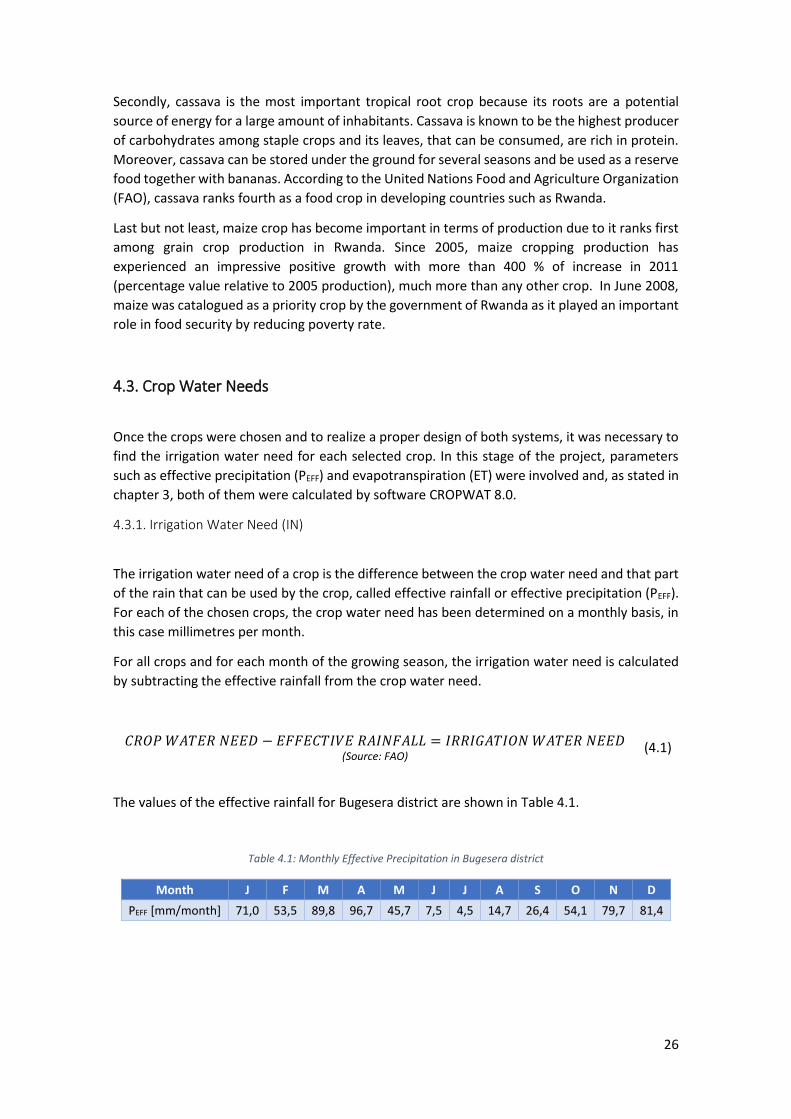


![Tesi de Màster - UPCommonsupcommons.upc.edu/bitstream/handle/2099.1/7192/MasterThesis Ameller.pdfSistemes Informàtics (LSI) [2] department of the Universitat Politècnica de Catalunya](https://static.documents.pub/doc/80x56/5f897b284562d7792a71504e/tesi-de-mster-amellerpdf-sistemes-informtics-lsi-2-department-of-the.jpg)


![CAN Ethernet Gateway - UPCommonsupcommons.upc.edu/.../26516/CAN_Ethernet_Gateway_Report.pdfFigure 4: Example of gateway sold by esd [1] Figure 5: Example of gateway sold by SYS TEC](https://static.documents.pub/doc/80x56/60a25061600fac242b0d03b8/can-ethernet-gateway-figure-4-example-of-gateway-sold-by-esd-1-figure-5-example.jpg)


