Water Supply System Performance for Different Pipe Materials Part I: Water Quality Analysis Silja Tamminen & Helena Ramos & Didia Covas Received: 13 January 2007 / Accepted: 10 January 2008 / Published online: 18 March 2008 # Springer Science + Business Media B.V. 2008 Abstract The quality of potable water has been a major issue in the water industry for the last few decades. The deterioration of treated water can be due to physical, chemical or microbiological changes that occur in the water during distribution. In addition, pipe material and decay of a disinfectant agent can affect the quality of the water being distributed. In this study the purpose was to simulate the decay of chlorine in two networks, one made of old cast iron (CI) pipes and another of polyethylene (PE) pipes. In addition the performance of the network considering chlorine concentration, velocity, water age, and an intrusion of a contaminant – in this case organic material – into the network was evaluated. The simulations were performed with EPANET software using as the simulation network an example network from the program. It was found that the CI network requires higher initial chlorine concentrations than the PE network to maintain the required minimum chlorine concentration throughout the whole network. To maintain the chlorine concentrations required by WHO (Cl must be greater than 0.2 mg/l and lesser than 0.5 mg/l) re- chlorination stations were necessary to add into both networks. The performance of both networks before re-chlorination was low due to high initial chlorine concentrations, but after the addition of the re-chlorination stations it was 100% throughout the networks. The performance of the velocities was good in both networks. The performance of the water age was dependent mainly on the tank usage, and the performance of contamination by organic material depended on the coefficient that defines the decay rate of the organic material in the bulk phase. Water Resour Manage (2008) 22:1579–1607 DOI 10.1007/s11269-008-9244-x DO9244; No of Pages S. Tamminen : H. Ramos (*) : D. Covas Instituto Superior Técnico, Av. Rovisco Pais, 1049-001 Lisbon, Portugal e-mail: [email protected]S. Tamminen e-mail: [email protected]D. Covas e-mail: [email protected]
Transcript
Water Supply System Performance for Different PipeMaterials Part I: Water Quality Analysis
Silja Tamminen & Helena Ramos & Didia Covas
Received: 13 January 2007 /Accepted: 10 January 2008 /Published online: 18 March 2008# Springer Science + Business Media B.V. 2008
Abstract The quality of potable water has been a major issue in the water industry for thelast few decades. The deterioration of treated water can be due to physical, chemical ormicrobiological changes that occur in the water during distribution. In addition, pipematerial and decay of a disinfectant agent can affect the quality of the water beingdistributed. In this study the purpose was to simulate the decay of chlorine in two networks,one made of old cast iron (CI) pipes and another of polyethylene (PE) pipes. In addition theperformance of the network considering chlorine concentration, velocity, water age, and anintrusion of a contaminant – in this case organic material – into the network was evaluated.The simulations were performed with EPANET software using as the simulation network anexample network from the program. It was found that the CI network requires higher initialchlorine concentrations than the PE network to maintain the required minimum chlorineconcentration throughout the whole network. To maintain the chlorine concentrationsrequired by WHO (Cl must be greater than 0.2 mg/l and lesser than 0.5 mg/l) re-chlorination stations were necessary to add into both networks. The performance of bothnetworks before re-chlorination was low due to high initial chlorine concentrations, butafter the addition of the re-chlorination stations it was 100% throughout the networks. Theperformance of the velocities was good in both networks. The performance of the water agewas dependent mainly on the tank usage, and the performance of contamination by organicmaterial depended on the coefficient that defines the decay rate of the organic material inthe bulk phase.
Water Resour Manage (2008) 22:1579–1607DOI 10.1007/s11269-008-9244-x
DO9244; No of Pages
S. Tamminen :H. Ramos (*) :D. CovasInstituto Superior Técnico, Av. Rovisco Pais, 1049-001 Lisbon, Portugale-mail: [email protected]
Keywords Water supply systems . Performance evaluation . Water quality . Pipe material
1 Introduction
Several factors can contribute to the deterioration of water quality during distribution, suchas interactions between the distributed water and pipe material or interactions within thebulk water (Kirmeyer et al. 2001). In addition, the decay of a disinfectant agent, such aschlorine, can degrade the microbial conditions of a distribution system causing thus apossible health risk to the consumers (Clark and Haught 2005).
Pressure variations caused by sudden changes in the flow velocity (LeChevallier et al.2003), originated from basic distribution system operations such as starting or stopping of apump (Gullick et al. 2004) can lead to the external pressure of the pipe exceeding theinternal pressure (Kirmeyer et al. 2001). In such situation, there is a chance of non-potablewater entering the distribution system from the surrounding environment (Loureiro 2002;Gullick et al. 2004) through leakage points, faulty seals or joints etc. (Kirmeyer et al. 2001),giving thus an opportunity for contaminants to enter the distribution system degrading thequality of the water (Gullick et al. 2004). It has also been found that flow velocity andchlorine decay rates in the bulk water correlate significantly, higher flow velocities leadingto higher decay rates (Menaia et al. 2002).
Increased residence time, especially in reservoirs, increases the turbidity and the bacterialnumbers of the distributed water (Kerneïs et al. 1995; Power and Nagy 1999). Chlorineresiduals decrease rapidly with distance from the treatment plant causing the furthest parts ofthe distribution system remaining with virtually no chlorine residuals leading thus to highbacterial numbers (Lu et al. 1995; DiGiano 2005). Also, the material of water piping affectsthe chlorine decay. Free chlorine can be consumed by the internal walls of the piping, byreactions with the fixed biomass on the pipe walls and with the pipe material itself (Frateuret al. 1999). In fact, pipe materials can be classified either having high reactivity, such asunlined iron, or low reactivity, such as PVC or MDPE (Hallam et al. 2002). The high reactivityof iron pipes might be due to the fact that free chlorine reacts readily with ferrous iron toproduce ferric hydroxide (Lu et al. 1995). Corrosion scales can also increase the chlorinedemand and offer a good environment for micro-organisms enhancing thus the growth ofbiofilms (Sander et al. 1996; Volk et al. 2000; Sarin et al. 2004; Clark and Haught 2005).
Chlorine is one of the most important disinfectant agents in water treatment. Chlorine isused either as free chlorine or as monochloramine to disinfect the bulk water in drinkingwater distribution systems and to control the growth of biofilms (Jegatheesan et al. 2000;Maier et al. 2000; Vikesland et al. 2001). It is important to maintain adequate chlorineresidual throughout the whole distribution system in order to sustain the chemical andmicrobial quality of distributed water (Vasconcelos et al. 1997; Munavalli and MohanKumar 2003). However, being a strong oxidiser, chlorine reacts readily with organic andinorganic compounds and thus decays inside the distribution system through reactions bothin the bulk phase and at the pipe wall (Vasconcelos et al. 1997; Kiéne et al. 1998; Powell etal. 2000a; Clark and Sivaganesan 2002; Munavalli and Mohan Kumar 2003; Clark andHaught 2005). In addition, chlorine can be consumed by the corrosion process of the pipematerial (Vasconcelos et al. 1997; Clark and Haught 2005) as well as due to the biofilmattached to the pipe wall. The decay caused by biofilms varies largely, however, and theinteractions between biofilms and disinfectants are still inadequately understood (Kiéne etal. 1998; Jegatheesan et al. 2000).
1580 S. Tamminen et al.
2 Mathematical Model for Chlorine Decay
Chlorine decay in distribution systems can be characterised as a combination of first-orderreactions in the bulk liquid and first-order or zero-order mass transfer-limited reactions atthe pipe wall (Vasconcelos et al. 1997). In water quality modelling tools chlorine decay isoften simplified to first-order kinetics:
C tð Þ ¼ C0e�kt ð1Þ
where t is time, C the chlorine concentration after time t, C0 the initial chlorineconcentration, and k the decay coefficient. The advantage of the first-order reaction schemeis its simplicity and available analytical solution (Kastl et al. 1999; Loureiro 2002) and thefact that there is need for only one decay coefficient, k (Maier et al. 2000). The decay ofchlorine in a distribution system is due to both bulk and wall decay (Munavalli and MohanKumar 2003) and the easiest method to define the overall decay coefficient is to use thesum of these two coefficients (Powell et al. 2000b; Loureiro 2002):
k ¼ kb þ kw ð2Þwhere kb is the bulk decay coefficient and kw is the wall decay coefficient. The bulk decayis due to chlorine reacting with chemicals in the bulk phase and the wall decay is due tochlorine reacting with biofilms, consumption of chlorine in the corrosion process and masstransport of chlorine between the bulk flow and pipe wall. The decay coefficients shoulddescribe these factors, thus they are site specific and are required to be verified by fieldmeasurements (Vasconcelos et al. 1997).
However, a more complex kinetic model for wall and bulk decay is used within theEPANET network modelling package. The kinetic model of EPANET tries to include to thedecay model the mass transfer mechanism by which the chlorine is transferred from the bulkflow to the pipe wall. Thus, kw turns into a function of velocity, pipe diameter, pipe length,diffusivity, and viscosity (Powell et al. 2000b). The decay coefficient used in EPANETmodelling package (Maier et al. 2000):
k ¼ kb þ kfkwRH kf þ kwð Þ ð3Þ
Where kf is a flow dependent mass transfer coefficient, kb and kw are parametersrepresenting bulk and wall demand, respectively, and RH is the hydraulic radius. The decayrate coefficients, both the bulk decay and the wall decay, for chlorine can have a largevariability. In literature values between 0.02–0.74 h−1 (Powell et al. 2000a; Hallam et al.2003) and 0.01 h–0.78 h−1 (Hallam et al. 2002) have been reported for bulk decaycoefficient (first order) and wall decay coefficient (first order), respectively. The variation inthe bulk decay coefficient is due to quality changes in the water and the wall decaycoefficient varies according to the material and the condition of the pipe (Powell et al.2000a; Hallam et al. 2002, 2003).
The aim of this work was to simulate chlorine decay in two different networks – anetwork that consists solely of CI pipes and a network consisting of PE pipes – in order toestimate the necessary chlorine dosage to maintain the required chlorine concentrationsthroughout the network. In addition, the performance of the networks regarding chlorineconcentrations, velocity, water age and an intrusion of a contaminant into the network wasevaluated. The modelling tool used was the EPANET program that is available on theinternet at the page of USEPA (www.epa.gov).
Water supply system performance for different pipe materials 1581
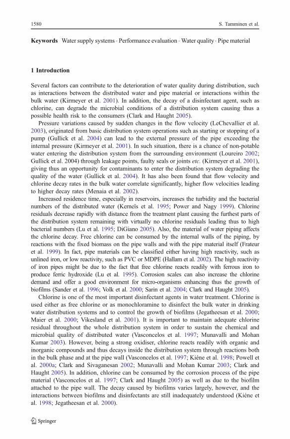
The network used in the simulations was an example network from the EPANET program,net3.net (Fig. 1) that consists of two reservoirs (RIVER, LAKE), two pumps and 3 tanks,117 pipes with diameters between 20 and 76 cm and 92 nodes. The added input values forthe water were bulk decay coefficient, wall decay coefficients and initial chlorineconcentrations in the reservoirs. Besides the chlorine concentration, the quality of thewater in the two reservoirs was identical, and it was not possible to set any othercharacteristics for the water. The input characteristics for the network tanks included onlydimensional characteristics without possibility of choosing their material.
The roughness coefficients were adjusted to fit a network made of 30 years old slightlycorroded CI pipes and another one of PE pipes. As bulk decay coefficient an average value ofthe values from the literature (Powell et al. 2000a; Hallam et al. 2003) was used, i.e. 0.36 h−1.As wall decay coefficients average values obtained by Hallam et al. 2002 were used, i.e.,0.67 h−1 for CI pipes and 0.05 h−1 for PE pipes. 1st order kinetic reactions for both bulk andwall decay were used. The roughness coefficients for CI pipes were calculated from Walski1984 and the roughness coefficients for PE pipes were adjusted using the values from Walski1984 and Rossman 2000. The roughness coefficients (Hazen-Williams, C) for the CI networkvaried between 108 and 118 and for the PE network between 140 and 144 depending on thepipe diameter.
According to the WHO the concentration of chlorine in a distribution network shouldremain between 0.2 and 0.5 mg/l (Loureiro 2002). Thus, three sets of simulations were runfor both networks. The first simulation was done to find out the lowest initial chlorineconcentrations necessary to maintain the minimum required chlorine concentrationthroughout the whole distribution system. The second simulation was done to find thenecessary locations for re-chlorination to maintain the chlorine concentration betweenthe recommended limits. Thirdly, the water age of the two systems was simulated. For thechlorine levels, the simulation was run for 6 weeks (1,008 h) and for the water age for36 weeks (6,048 h) for the network to reach equilibrium.
RIVER LAKE
TANK 1
TANK 2
TANK 3
Fig. 1 General layout of thesimulation network
1582 S. Tamminen et al.
3.2 Results and Discussion
3.2.1 Chlorine
For the CI network the initial chlorine concentrations necessary to maintain the minimumchlorine concentration were 3.7 mg/l for the RIVER-reservoir and 2.6 mg/l for the LAKE-reservoir and for the PE network the corresponding values were 0.5 mg/l and 1.6 mg/l. Whencomparing the reaction rates (Fig. 2) for the two networks it can be seen that in the CI networkmajority of the chlorine decay occurs in the pipe wall (69.25%) and in the PE network in thebulk water (62.37%). This is due to the fact that the wall decay coefficient for CI pipes ismuch higher than for PE pipes the bulk decay coefficient being same for the two.
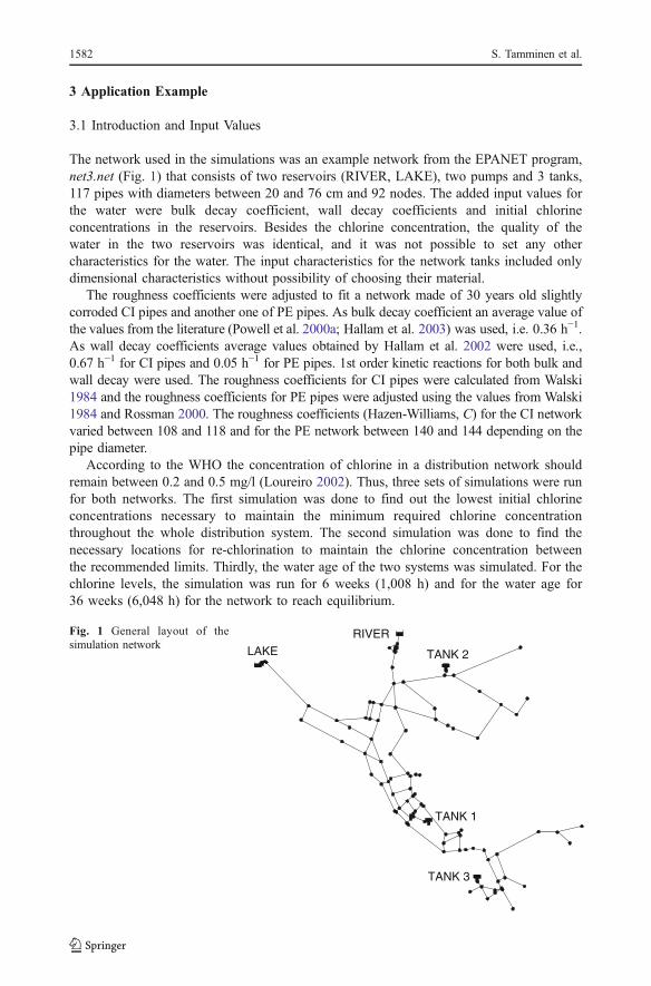
The consumption in the network system is based on five demand patterns (Fig. 3), whichare defined for 4 nodes presented in Fig. 4 (nodes 123, 15, 35 and 203), and the generaldefault demand pattern, which is defined for the rest of the nodes. The multiplier of thepatterns is the value that the base demand of each node is multiplied to generate effectivedemand. In nodes that have a specified demand pattern the base demand is 1 and the rest ofthe nodes have variable base demand. The system flow plot shows the overall consumptionin the network during a period of 24 h and this figure (Fig. 5) shows the peak and thelowest consumption hour. By drawing the contour plots for the chlorine concentration forthe hours of peak and lowest consumption, the differences between the behaviours of CIand PE networks considering chlorine decay can be seen. The contour plots (Figs. 6 and 7)show that majority of the network area in both networks has chlorine concentrations abovethe WHO recommendation limit 0.5 mg/l. At the peak hour 97% and 80% of the nodeshave chlorine concentrations above 0.5 mg/l in CI and PE networks, respectively. At thelowest consumption hour the corresponding percentages are 98% and 74%.
In the CI network the chlorine concentrations during maximum consumption are lowerthan the concentrations during minimum consumption. As EPANET includes the masstransfer mechanism to the chlorine decay and thus the decay is influenced by the ratechlorine is transferred from the bulk flow to the pipe wall; since most of the decay ofchlorine in the CI network occurs in the pipe wall; and since the decay coefficient is afunction of velocity, pipe diameter, pipe length, diffusivity, and viscosity (Powell et al.2000b) the higher chlorine concentrations during maximum consumption might beexplained with higher flow velocity and thus more efficient transport of chlorine to thepipe wall. It has been suggested that in pipes that react readily with chlorine (e.g. CI pipes)the wall decay is limited by the transfer of chlorine to the pipe wall and, in addition, apositive relationship between flow velocity and wall decay has been found (Hallam et al.
Bulk 21.2 %
Wall 69.25 %Tanks9.55 %
Bulk 62.37 %
Wall 21.22 %
Tanks16.41 %
Fig. 2 Reaction report for CIpipes (left) and PE-pipes
Water supply system performance for different pipe materials 1583
Fig. 3 From left to right General default demand pattern, demand pattern for node 123, node 15, node 35and node 203
LAKE
RIVER
NODE123
NODE 15
NODE 35 NODE 203
Fig. 4 Demand pattern nodes
1584 S. Tamminen et al.
2002). Thus, in the high consumption times the velocity of the fluid in the network is higherand chlorine is transported more efficiently to the pipe wall increasing the chlorine decay atthe pipe wall and resulting in lower chorine concentrations.
In the PE network the situation is opposite the peak hour having higher chlorineconcentrations than low consumption hour. This is probably due to the chlorine decay in thebulk phase, which has much higher consumption of chlorine than the pipe wall. In lowconsumption periods the flow velocity is low giving thus time for the bulk reactions tooccur. It should be noted that the area with chlorine concentrations below 0.2 mg/l in thecontour plots of the PE-network are due to a tank (TANK 2), which stops functioninghaving thus no in- or outflow and consequently chlorine levels constantly at zero.
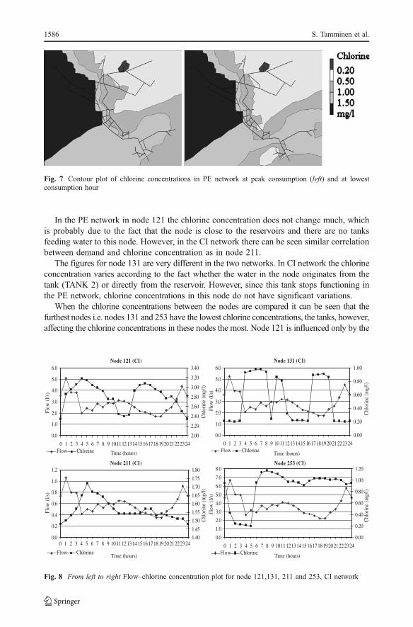
By plotting the chlorine concentration with the demand in a single node the behaviour ofthe chlorine concentration compared to the demand can be seen (Figs. 8 and 9). These plotswere drawn for four nodes in different parts of the network (Fig. 10) and they show that thebiggest influence on the chlorine concentration is the fact whether the water in the nodeoriginates from a tank or directly from a reservoir. These figures show that in node 253there are big variations in the chlorine concentration which are due to the fact that water, atthe low chorine concentration hours, enters the node from a tank (TANK 3).
In node 211 in the CI network chlorine concentration correlates with the demand, lowdemand hours having high chlorine concentrations and vice versa. This behaviour is probablydue to the low flow velocity at low demand hours and thus smaller wall decay. This behaviourcan not be seen in the PE network, probably due to the less significant wall decay. However,in the PE network the chlorine concentrations are high with high demand and low with lowdemand. This might follow from the fact that at low consumption hours there is time for thebulk decay to occur which in the PE network is the main reason for the chlorine decay.
Fig. 6 Contour plot of chlorine concentrations in CI network at peak consumption (left) and at lowestconsumption hour
Water supply system performance for different pipe materials 1585
In the PE network in node 121 the chlorine concentration does not change much, whichis probably due to the fact that the node is close to the reservoirs and there are no tanksfeeding water to this node. However, in the CI network there can be seen similar correlationbetween demand and chlorine concentration as in node 211.
The figures for node 131 are very different in the two networks. In CI network the chlorineconcentration varies according to the fact whether the water in the node originates from thetank (TANK 2) or directly from the reservoir. However, since this tank stops functioning inthe PE network, chlorine concentrations in this node do not have significant variations.
When the chlorine concentrations between the nodes are compared it can be seen that thefurthest nodes i.e. nodes 131 and 253 have the lowest chlorine concentrations, the tanks, however,affecting the chlorine concentrations in these nodes the most. Node 121 is influenced only by the
Fig. 7 Contour plot of chlorine concentrations in PE network at peak consumption (left) and at lowestconsumption hour
Fig. 8 From left to right Flow–chlorine concentration plot for node 121,131, 211 and 253, CI network
1586 S. Tamminen et al.
RIVER reservoir and has thus, in both networks, chlorine concentrations that are still reasonablyclose to the initial chlorine concentrations in the reservoir. On the other hand, node 211 isinfluenced by both reservoirs and has thus, in the PE network, higher chlorine concentration thannode 121, even though it is further in the distribution system,which is evidently due to the fact thatthe initial chlorine concentration in the LAKE reservoir is somewhat higher than in the RIVERreservoir. This behaviour does not take place in the CI network since the RIVER reservoir hashigher initial chlorine concentration than the LAKE reservoir.
Fig. 9 From left to right Flow–chlorine concentration plot for node 121, 131, 211 and 253, PE network
LAKE RIVER
NODE 121
NODE 211
NODE 253
NODE 131Fig. 10 Scheme of the simula-tion network with the nodes inquestion
Water supply system performance for different pipe materials 1587
3.2.2 Re-chlorination
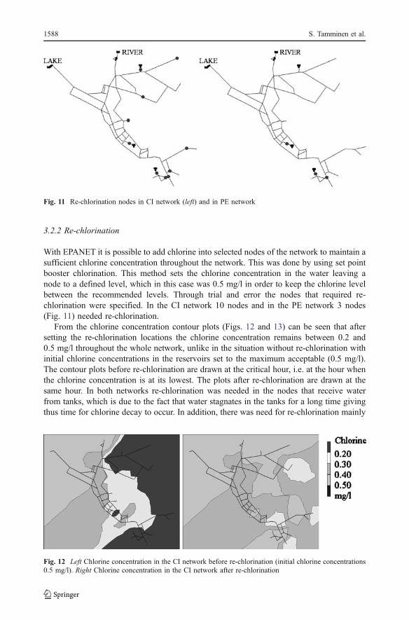
With EPANET it is possible to add chlorine into selected nodes of the network to maintain asufficient chlorine concentration throughout the network. This was done by using set pointbooster chlorination. This method sets the chlorine concentration in the water leaving anode to a defined level, which in this case was 0.5 mg/l in order to keep the chlorine levelbetween the recommended levels. Through trial and error the nodes that required re-chlorination were specified. In the CI network 10 nodes and in the PE network 3 nodes(Fig. 11) needed re-chlorination.
From the chlorine concentration contour plots (Figs. 12 and 13) can be seen that aftersetting the re-chlorination locations the chlorine concentration remains between 0.2 and0.5 mg/l throughout the whole network, unlike in the situation without re-chlorination withinitial chlorine concentrations in the reservoirs set to the maximum acceptable (0.5 mg/l).The contour plots before re-chlorination are drawn at the critical hour, i.e. at the hour whenthe chlorine concentration is at its lowest. The plots after re-chlorination are drawn at thesame hour. In both networks re-chlorination was needed in the nodes that receive waterfrom tanks, which is due to the fact that water stagnates in the tanks for a long time givingthus time for chlorine decay to occur. In addition, there was need for re-chlorination mainly
Fig. 12 Left Chlorine concentration in the CI network before re-chlorination (initial chlorine concentrations0.5 mg/l). Right Chlorine concentration in the CI network after re-chlorination
Fig. 11 Re-chlorination nodes in CI network (left) and in PE network
1588 S. Tamminen et al.
in the remote nodes of the network. It should be noted, though, that the most remote nodesof the network are not dead ends, but instead nodes with demand from where water isdistributed further to the consumers, which is why re-chlorination in these nodes isjustifiable.
3.2.3 Water Age
Water age is the time that a water parcel spends in the network. New water entering thenetwork from reservoirs is considered to have water age of zero (Rossman 2000). It isimportant to know the water age of a distribution system in order to estimate the extent ofchlorine decay or disinfection by-product formation. If the residence time is known it iseasier for water utilities to e.g. decide the location of sampling stations (DiGiano et al.2005). The water age simulations were done to compare the chlorine concentrations and thewater age in the network. The obtained water ages are presented in the contour plots(Figs. 14 and 15) at peak and low consumption hour.
The average water ages at the peak and low consumption hour in the CI network are33.14 h and 13.48 h, respectively. The high water age at the peak consumption hour is dueto the fact that all three tanks are providing water with high age to the network. On thecontrary, at the low consumption hour, the tanks are filling up and water to the network is
Fig. 14 Contour plot of water age in CI network at the peak consumption hour (left) and at the lowestconsumption hour
Fig. 13 Left Chlorine concentration in the PE network before re-chlorination (initial chlorine concentrations0.5 mg/l). Right Chlorine concentration in the PE network after re-chlorination
Water supply system performance for different pipe materials 1589
provided directly from the reservoirs with small water age. For PE network the averagewater ages are 7.50 and 16.93 h, for peak and low consumption, respectively. The tankusage in PE network is not as significant as in the CI network and it does not have such aneffect on the water age. Thus, the water age in the PE network is low when the consumptionis at its highest and vice versa.
By comparing the plot of water age and chlorine concentration of the CI network at peakhour it can be seen that where the water age is highest, the chlorine concentrations are lowestsince the distributed water is originating from the tanks. This is the case at the low consumptionhour as well. For PE network similar behaviour can be seen. In the PE network, however,longer stagnation times lead to higher chlorine decay due to the decay in the bulk phase.
4 Performance Evaluation
4.1 Introduction
The level of service provided by water supply and distribution systems is one of the keyissues facing the water industry today. However, measuring the performance of adistribution network is not a straightforward task, given the multiple factors involved,and the lack of a unified approach or a single clear-cut definition of performance. In orderto evaluate the service of a water supply there has been developed a PerformanceEvaluation System. The Performance Evaluation System is a technical analysis tool basedon a system of penalty curves, providing standardised means of diagnosis (Coelho 1997).
The method is defined by three types of units. Firstly it is defined by the numerical valueof a network property or condition variable, which is considered to be showing the
0
25
50
75
100
0.00 0.10 0.20 0.50 0.80 4.00
Chlorine (mg/l)
Perf
orm
ance
(%
)
Fig. 16 Penalty function forchlorine
Fig. 15 Contour plot of water age in PE network at the peak consumption hour (left) and at the lowestconsumption hour
1590 S. Tamminen et al.
particular aspect being examined. Secondly, it is defined by the penalty curve which plotsthe value of a performance attributed to the condition variable or network property. Theperformance index varies between a no-service (0%) and an optimum-service (100%)situation, and the curves are supposed to penalise any deviation from the latter. Theconvention adopted in this work uses a 0 to 100% scale, with the following meanings:100% – optimum service, 75% – adequate service, 50% – acceptable service, 25% –unacceptable service and 0% – no service. Thirdly, the method is defined by a networkoperator which allows the performance values at element level to be aggregated across thenetwork or parts of it (Coelho 1997).
Thus, in order to aggregate the performances at element level across the network anaggregation function is defined (Eq. 4). This function represents the importance of eachelement related to the system as a whole.
P ¼ W pmið Þ ¼XN
i¼1
wi � pmið Þ ð4Þ
where P is the global value of performance, pmi the performance in each element i, and wi
the weight of each element according to Eq. 5:
wi ¼ ziPN
i¼1zi
ð5Þ
where zi is the element used (Araujo 2005).Hence, this method yields values of performance evaluation for every element of a
network as well as for the network as a whole. There is a global value (P) which is achievedthrough a particular function in order to represent the performance assessment of thenetwork, and, on the other hand, a population of elementary values (pmi) which lends itselfto a basic statistical treatment. The two are combined together graphically in diagramswhere performance is plotted against simulation period, typically a 24-h simulation insteady state conditions. The main curve represents the global performance, whereas theshaded areas are 25% demand percentile bands which should be read as follows: if (t,y) arethe coordinates of a given point in the P% demand percentile curve it means that at time t P% of the total demand are being supplied with a performance that is smaller or equal to y(Coelho 1997).
Fig. 17 Performance of chlorine in the CI network in minimum hour (left) and peak hour
Water supply system performance for different pipe materials 1591
4.2 Performance Analysis before Re-chlorination
4.2.1 Chlorine
The performance analysis before re-chlorination was done with initial chlorine concen-trations in the RIVER and LAKE reservoirs, for the CI network 3.7 and 2.6 mg/l, and forthe PE network 0.5 and 1.6 mg/l, respectively. The penalty function was adapted fromCoelho and Alegre (1999) and it can be seen in Fig. 16. Since the chlorine concentrationshould maintain between 0.2 and 0.5 mg/l throughout the network, the performance in thepenalty function maintains at 100% with these chlorine concentration values. Chlorineconcentration values below the minimum limit 0.2 mg/l yield a performance of 0%. Whenthe chlorine concentration values exceed the recommended upper limit 0.5 mg/l theperformance descend to 25% and maintains in this value.
The performance of the network with the above mentioned initial chlorine concen-trations is very low especially in the CI network. This is because majority of the CI networkhas chlorine concentrations above the accepted upper limit, 0.5 mg/l. In the PE network thesituation is better due to lower initial chlorine concentrations.
In the CI network (Fig. 19) the performance maintains always equal or above 25% sincethe initial chlorine doses are set so that the chlorine concentration does not fall under0.2 mg/l. However, the performance of the network is only 25% throughout the wholesimulation cycle with low and average demand (<75%), which is due to chlorine
Fig. 19 Performance simulation diagram for chlorine in the CI network (left) and in the PE network
Fig. 18 Performance of chlorine in the PE network in minimum hour (left) and peak hour
1592 S. Tamminen et al.
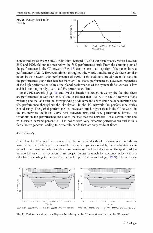
concentrations above 0.5 mg/l. With high demand (>75%) the performance varies between25% and 100% falling at times below the 75% performance limit. From the contour plots ofthe performance in the CI network (Fig. 17) can be seen that majority of the nodes have aperformance of 25%. However, almost throughout the whole simulation cycle there are alsonodes in the network with performance of 100%. This leads to a broad percentile band inthe performance graph that reaches from 25% to 100% performances. However, regardlessof the high performance values, the global performance of the system (index curve) is lowand it is running barely over the 25% performance limit.
In the PE network (Figs. 18 and 19) the situation is better. However, the fact that thereare performances lower than 25% is due to the fact that TANK 3 in the PE network stopsworking and the tank and the corresponding node have thus zero chlorine concentration and0% performance throughout the simulation. In the PE network the performance variesconsiderably. The global performance is, however, much higher than in the CI network; inthe PE network the index curve runs between 50% and 75% performance limits. Thevariations in the performance are due to the fact that the network – at a certain hour andwith certain demand percentile – has nodes with very different performances and is thusfairly heterogeneous leading to percentile bands that are very wide at times.
4.2.2 Velocity
Control on the flow velocities in water distribution networks should be maintained in order toavoid structural problems or undesirable hydraulic regimes caused by high velocities, or inorder to minimise the unfavourable consequences of too low velocities on the quality of thetransported water. It is common to use project criteria in which the reference velocity Vref iscalculated according to the diameter of each pipe (Coelho and Alegre 1999). The reference
0 to 25% 25 to 50% 50 to 75% 75 to 100% Index curve
Fig. 21 Performance simulation diagram for velocity in the CI network (left) and in the PE network
0
25
50
75
100
0 0.3 Vref 2.0 Vref 3.0 Vref 7.0 Vref
Velocity (m/s)
Perf
orm
ance
(%
)
Fig. 20 Penalty function forvelocity
Water supply system performance for different pipe materials 1593
velocity is considered to be the optimum velocity for a certain pipe, thus the performance forthe reference velocity is 100% (Fig. 20). The following expression (Eq. 6) according to DR23/95 (1995), Article 21 is proposed for the reference velocity of a pipe with diameter D.
Vref ¼ 0:1274D0:4 ð6Þwhere D is the diameter of the pipe (in mm) and Vref is in m/s (Coelho and Alegre 1999). Theminimum norm velocity is 0.3 m/s (DR 23/95 1995), returning thus a performance of 75%.Vref being the ideal velocity returns performance of 100%.
When considering the flow velocity the performance graphs are fairly similar for thetwo networks the differences being probably due to roughness coefficients. The globalperformance curve in both networks is in the region of 75% performance limit, thereforethe performance in both networks can be considered good. It can be seen from Fig. 21that the performance with higher (>50%) demand is, in both networks, always clearlyover 75%. In the PE network the performance reaches 100% limit, unlike in the CInetwork, which indicates that the reference velocity is not obtained in the CI network.Also, with lower (<50%) demand the performance maintains always above 25%, whichmeans that velocities that are three – or more – times the reference velocity are never reachedin neither of the networks (Figs. 22 and 23).
Fig. 23 Performance of velocity in the PE network in minimum hour (left) and peak hour
Fig. 22 Performance of velocity in the CI network in minimum hour (left) and peak hour
1594 S. Tamminen et al.
4.3 Performance Analysis after Re-chlorination
In the performance analysis with re-chlorination stations the performance of bothnetworks considering chlorine concentrations was 100% throughout the whole simulationperiod. The performance considering velocities maintained identical to the performancebefore re-chlorination.
4.4 Performance Analysis for Water Age
Since the water age of a network depends on many variables such as length of the network,consumption, and the presence of tanks there are no explicit penalty functions for waterage. Thus, in order to see the performance of the water age in the network, the analysis wasdone with three different penalty functions to perform sensitivity analysis. The three penaltyfunctions are presented in Fig. 24.
0 to 25% 25 to 50% 50 to 75% 75 to 100% Index curve
0
25
50
75
100
Time (h)
Per
form
ance
(%
)
0 to 25% 25 to 50% 50 to 75% 75 to 100% Index curve
Fig. 25 From left Performance simulation diagram for water age in the CI network according to penaltyfunction I, II and III
0
25
50
75
100
0 5 10 15 20 25 30
Water Age (h)
Per
form
ance
(%
)
0
25
50
75
100
0 20 50 60 80 100
Water Age (h)
Per
form
ance
(%
)
0
25
50
75
100
0 50 100 150 200 250 300 350
Water Age (h)
Per
form
ance
(%
)
Fig. 24 From left Penalty function I, II and III for water age
Water supply system performance for different pipe materials 1595
By comparing the graphs in Figs. 25 and 26 it can be seen that the performance changesa lot more in the CI network than in the PE network. In the CI network the changes occurmainly at times of higher consumption whereas in the PE network the performancemaintains virtually identical with different penalty functions. This is most likely due to thefact that in the CI network at the peak consumption hours the tanks are providing thenetwork water with very high water age while in the PE network the tanks are less used. Inthe PE network the performance is good throughout the simulation cycle the globalperformance maintaining in all three situations above 75% performance limit and in the twolatter cases constantly at 100% with average and high demand (>25%). In the CI network
0 to 25% 25 to 50% 50 to 75% 75 to 100% Index curve
0
25
50
75
100
Time (h)
Per
form
ance
(%
)
0 to 25% 25 to 50% 50 to 75% 75 to 100% Index curve
Fig. 26 From left Performance simulation diagram for water age in the PE network according to penaltyfunction I, II and III
1596 S. Tamminen et al.
with penalty curve I the global performance at high consumption hours descends below theperformance limit of 50% maintaining nevertheless above 75% performance limit at timesof low consumption. These drops in the global performance obviously lessen when thewater age in the penalty curves increases i.e. in the two latter cases. In the last case theperformance in the CI network is already very good; the index curve stays close to 100%and the performance with average and high demand (>25%) maintains at 100%.
4.5 Performance Analysis with Leak
4.5.1 Introduction
In these simulations a leak was created in three nodes. The purpose was to see, whether aleak will cause changes in the chlorine concentration or flow velocity of the network. Thepenalty functions used in these simulations were identical to the ones in previoussimulations. A leak was simulated in three nodes; in the node with the highest elevation(node 153, elevation 22.18 m), the node with lowest elevation (node 167, elevation
0 to 25% 25 to 50% 50 to 75% 75 to 100% Index curve
Fig. 28 Performance simulation diagram for velocity in the CI network (left) and in the PE network withleak in node 203
Water supply system performance for different pipe materials 1597
−1.52 m) and the node with biggest demand (node 203, elevation 0.61 m). Each of the leakswas simulated separately i.e. only one of the nodes had a eak at a time.
In order to simulate a leak in the EPANET program it is necessary to introduce an emitter in anode. Emitters are devices that can be used to model flow through an orifice that discharges tothe atmosphere and they can thus be used to simulate leakage in a pipe connected to the node.The flow rate through the emitter can be calculated with: (Rossman 2000)
q ¼ Cpa ð7Þwhere q is the flow rate, p is pressure, C is the emitter coefficient of the orifice, whichdepends on the shape and the diameter of the orifice and α is the pressure exponent(Colombo and Karney 2002; Araujo et al. 2006). When an emitter is used to simulate leakageit is necessary to introduce the emitter exponent, α, and the emitter coefficient C as inputvalues. For nozzles and sprinkler heads the emitter exponent α is often assigned a value of0.5 to reflect flow through a fixed size orifice (Colombo and Karney 2002). However, othervalues have been suggested. Araujo et al. (2003) used the value 1.18. They suggest that eventhough this value is quite a bit higher than the expectable 0.5 it is nevertheless found byexperimental results that it can be applied and that the difference in α may be caused bychanges in the shape and size of the cracks and orifices due to the internal or externalpressure differences.
Thus, when performing the simulations with the leak, a leak of 25% was simulated ineach node (Colombo and Karney 2002). With emitter exponent of 1.18 and demand of125% the emitter coefficients for each situation were found. The emitter coefficients fornode 153 were 0.1 and 0.1 for CI and PE network, respectively, for node 167 0.03 and 0.02
Fig. 31 Organic material propagation in CI (left) and PE network at critical hour (node 101, Bulk coeff.−0.1)
0
25
50
75
100
0 5 10 15 20 30 50Organic Material (mg/l)
Per
form
ance
(%
)
0
25
50
75
100
0 5 10 15 20 40 50
Organic Material (mg/l)
Per
form
ance
(%
)
0
25
50
75
100
0 5 10 15 20 25 50
Organic Material (mg/l)
Per
form
ance
(%
)
Fig. 30 From left Penalty function I, II and III for organic material contamination
1598 S. Tamminen et al.
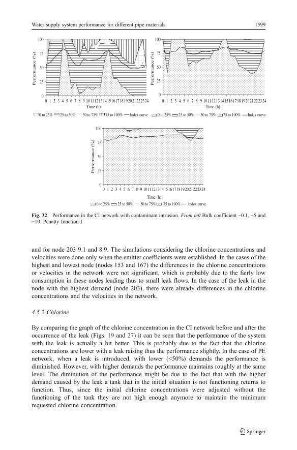
and for node 203 9.1 and 8.9. The simulations considering the chlorine concentrations andvelocities were done only when the emitter coefficients were established. In the cases of thehighest and lowest node (nodes 153 and 167) the differences in the chlorine concentrationsor velocities in the network were not significant, which is probably due to the fairly lowconsumption in these nodes leading thus to small leak flows. In the case of the leak in thenode with the highest demand (node 203), there were already differences in the chlorineconcentrations and the velocities in the network.
4.5.2 Chlorine
By comparing the graph of the chlorine concentration in the CI network before and after theoccurrence of the leak (Figs. 19 and 27) it can be seen that the performance of the systemwith the leak is actually a bit better. This is probably due to the fact that the chlorineconcentrations are lower with a leak raising thus the performance slightly. In the case of PEnetwork, when a leak is introduced, with lower (<50%) demands the performance isdiminished. However, with higher demands the performance maintains roughly at the samelevel. The diminution of the performance might be due to the fact that with the higherdemand caused by the leak a tank that in the initial situation is not functioning returns tofunction. Thus, since the initial chlorine concentrations were adjusted without thefunctioning of the tank they are not high enough anymore to maintain the minimumrequested chlorine concentration.
0 to 25% 25 to 50% 50 to 75% 75 to 100% Index curve
0
25
50
75
100
Time (h)
Per
form
ance
(%
)
0 to 25% 25 to 50% 50 to 75% 75 to 100% Index curve
Fig. 32 Performance in the CI network with contaminant intrusion. From left Bulk coefficient −0.1, −5 and−10. Penalty function I
Water supply system performance for different pipe materials 1599
4.5.3 Velocity
Considering the velocities the changes in the CI network are small (Figs. 23 and 28). Withhigher (>50%) demand the performance maintains virtually identical. The changes happenin the lower percentiles; the performance with low (<25%) demand improves slightly. In thePE network there are changes even in the higher demand percentiles. The performance withhigher (>50%) demand improves slightly. The changes with lower (<50%) demand can beconsidered insignificant. The global performance maintains virtually at the sameperformance level in both networks.
4.6 Performance Analysis with an Intrusion of Organic Material into the Network
4.6.1 Introduction
Simulating contaminant intrusion into the network in EPANET can be done by eithersimulating a contaminant that is non-reactive or a contaminant that is reactive. When acontaminant that is reactive is simulated it is necessary to know the reactions that thecontaminant has with the bulk water and the pipe wall in order to adjust the reactionkinetics and reaction coefficients. In this case the purpose was to simulate an intrusion oforganic material that reacts with the chlorine present in the network. First order reactionkinetics were used for the bulk water and the reactions at the pipe wall were neglected. Thesimulations were done with three different bulk coefficients; −0.1, −5 and −10 to see thedifferent behaviour of the contaminant. The intrusion was done using the setpoint booster
0 to 25% 25 to 50% 50 to 75% 75 to 100% Index curve
0
25
50
75
100
Time (h)
Per
form
ance
(%
)
0 to 25% 25 to 50% 50 to 75% 75 to 100% Index curve
Fig. 33 Performance in the PE network with contaminant intrusion. From left Bulk coefficient −0.1, −5 and−10. Penalty function I
1600 S. Tamminen et al.
source which sets the water leaving the node to have a certain concentration of contaminantwhich in this case was 50 mg/l.
The intrusion of organic material into the network was simulated in two nodes: node101 which is a node that is located close to the LAKE reservoir and has a fairly highelevation (12.8 m) and node 153 which is the node that has the lowest pressure in thenetwork. Node 101 was selected to have the intrusion for its elevation and the fact that itprovides water nearly to the whole network. This way the contamination spreads to alarge part of the network. Node 153 was chosen because of its low pressure and thus therisk of having a rupture and further easy access of the organic material to enter thedistribution system. The nodes are presented in Fig. 29. Due to the lack of an explicitpenalty function the performance analysis was done with three different penalty functionsto perform sensitivity analysis. The penalty curves for the organic material intrusion arepresented in Fig. 30.
4.6.2 Intrusion in Node 101
The propagation of the organic material in the network is presented in Fig. 31. From theperformance graphs (Figs. 31, 32, 33, 34, 35, 36 and 37) can be seen that the globalperformance in both networks improves when the bulk coefficient decreases i.e. with bulkcoefficient −10 the performance is better than with coefficient −0.1. This is due to the factthat the contaminant with smaller bulk coefficient is consumed faster in the network.
When the situation with penalty function I is considered, in the CI network withcoefficient −10 and −5 the global performance of the network is above the limit of 75%,
0 to 25% 25 to 50% 50 to 75% 75 to 100% Index curve
0
25
50
75
100
Time (h)
Per
form
ance
(%
)
0 to 25% 25 to 50% 50 to 75% 75 to 100% Index curve
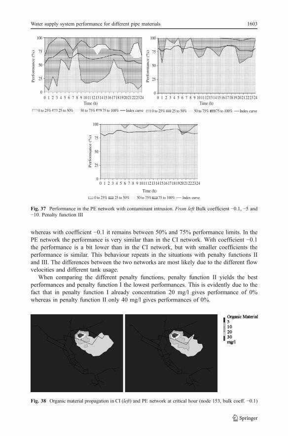
Fig. 36 Performance in the CI network with contaminant intrusion. From left Bulk coefficient −0.1, −5 and−10. Penalty function III
1602 S. Tamminen et al.
whereas with coefficient −0.1 it remains between 50% and 75% performance limits. In thePE network the performance is very similar than in the CI network. With coefficient −0.1the performance is a bit lower than in the CI network, but with smaller coefficients theperformance is similar. This behaviour repeats in the situations with penalty functions IIand III. The differences between the two networks are most likely due to the different flowvelocities and different tank usage.
When comparing the different penalty functions, penalty function II yields the bestperformances and penalty function I the lowest performances. This is evidently due to thefact that in penalty function I already concentration 20 mg/l gives performance of 0%whereas in penalty function II only 40 mg/l gives performances of 0%.
0 to 25% 25 to 50% 50 to 75% 75 to 100% Index curve
0
25
50
75
100
Time (h)
Per
form
ance
(%
)
0 to 25% 25 to 50% 50 to 75% 75 to 100% Index curve
Fig. 37 Performance in the PE network with contaminant intrusion. From left Bulk coefficient −0.1, −5 and−10. Penalty function III
Fig. 38 Organic material propagation in CI (left) and PE network at critical hour (node 153, bulk coeff. −0.1)
Water supply system performance for different pipe materials 1603
4.6.3 Intrusion in Node 153
When the organic material intrusion is simulated in node 153 the organic material doesn’tspread in a broad area in the network which can be seen in Fig. 38. Therefore, since thecontamination is only local the performance of the network maintains very high.Additionally, regardless of the penalty curve the performance in both networks maintainsvery similar. As an example in Fig. 39 there are presented the performance of bothnetworks with bulk coefficient −0.1 and penalty curve I. Changing the penalty curve or thebulk coefficient doesn’t cause significant changes to the performance of the networks.Thus, from the contour plots and the performance graphs it can be seen that theperformance in majority of the network is 100%, and thus the global performance curveruns close to 100% performance limit. However, since there are also some nodes in thenetwork that have high organic material concentration and therefore 0% performance, the25% demand percentile band is very wide reaching from performances of 0% toperformances of 100%.
5 Conclusions
The current paper presents mathematical model analysis for the calculation of water supplysystem performance with different pipe materials, as well as the developments regarding thewater quality assessment. The analysis of the results allows the following conclusions to bedrawn:
& For the CI-network higher initial chlorine concentrations are necessary compared toPE network in order to maintain the minimum acceptable chlorine level throughoutthe network.
& The need for higher initial chlorine concentrations in the CI network is possiblydue to higher wall decay rates.
& The fact that the CI network has low chlorine concentrations during maximumconsumption hours may be due to flow velocities enabling more efficienttransportation of chlorine to the pipe wall leading thus to higher chlorine decay rates.
& The low chlorine concentrations of the PE network during low consumption hoursare probably due to bulk reactions that in low consumption periods have more timeto occur. The wall decay in PE pipes is not such a significant factor.
0 to 25% 25 to 50% 50 to 75% 75 to 100% Index curve
Fig. 39 Performance in the CI network (left) and PE network with contaminant intrusion. Bulk coefficient−0.1. Penalty function I
1604 S. Tamminen et al.
& The most significant factor for the chlorine concentration in a specific node iswhether the water in the node originates from a tank or directly from a reservoir.However, when there is no effect of a tank the chlorine concentration correlateswith the demand in the node; for CI network the chlorine concentration is low inhigh demand hours and vice versa, and for PE network the chlorine concentrationis low in low demand hours and vice versa.
& In order to maintain the chlorine concentration between the recommended limits in thenetwork, when the initial chlorine concentration in the reservoirs is 0.5 mg/l, re-chlorination is required in certain nodes. In CI network the need for re-chlorination isbigger than in the PE network. Re-chlorination is needed in both networks in the nodesthat receive water from tanks and in some nodes in the furthest parts of the network.
& The performance considering chlorine concentrations in CI network is bad due tohigh chlorine consumption on the pipe wall and thus low chlorine levelsthroughout the network. In the PE network chlorine levels maintain higher dueto lower decay at the pipe wall and thus the performance maintains higher. Afterthe addition of re-chlorination stations the performance maintains at 100%throughout the whole simulation time in both networks.
& The water age in both networks corresponds logically with the chlorineconcentrations; at high water ages the chlorine concentrations are at lowest inboth networks. The performance of water age is mostly dependent on the usage ofthe tanks, which is why, due to lesser tank usage, the PE network has betterperformance. In the CI network, however, the performance is low mainly at thetimes of peak consumption hours, when the water to the network is largelyprovided from the tanks.
& The performance of the velocities of both networks is good throughout the wholesimulation without significant differences between the networks. This indicates thatthe network is not over- or under-dimensioned.
& Introduction of a leak into the network does not cause big changes in theperformance regarding the chlorine concentrations or velocities.
& The performance of the organic material intrusion is dependent on the bulkcoefficient, lower bulk coefficient leading to faster reaction rates, and thus lowerorganic material concentrations in the network.
Acknowledgements The authors wish to thank FCT (Portugal) through CEHIDRO (Hydraulic ResearchCentre from the Civil Engineering Department of Instituto Superior Técnico – from Technical University ofLisbon) and researchers projects POCTI/ECM/58375/2004 and PTDC/ECM/65731/2006 (partly supportedby funding under the European Commission – FEDER) for financial and all type of support that allowed thedevelopment of this research work.
References
Araujo L (2005) Losses Control in Sustainable Management of Water Supply Systems. Ph.D. Thesis,Instituto Superior Técnico, Lisbon, Portugal (in Portuguese)
Araujo LS, Coelho ST, Ramos HM (2003) Estimation of distributed pressure-dependent leakage andconsumer demand in water supply networks. CCWI (Computing and Control for the Water Industry),Imperial College, UK
Araujo LS, Ramos H, Coelho ST (2006) Pressure control for leakage minimisation in water distributionsystems management. Water Resour Manag 20(1):133–149
Water supply system performance for different pipe materials 1605
Clark RM, Haught MC (2005) Characterizing pipe wall demand: implications for water quality modeling. JWater Resour Plan Manage 131(3):208–217
Clark RM, Sivaganesan M (2002) Predicting chlorine residuals in drinking water: second order model. JWater Resour Plan Manage 128(2):152–161
Coelho ST (1997) Performance assessment through mathematical modelling. Workshop on PerformanceIndicators for Transmission and Distribution Systems, IWSA, Associação Internacional dos Distrib-uidores de Água, National Laboratory of Civil Engineering, Lisbon, Portugal
Coelho ST, Alegre H (1999) Performance indicators of water supply systems. National Laboratory of CivilEngineering, Lisbon, Portugal (in Portuguese)
Colombo AF, Karney BW (2002) Energy and costs of leaky pipes: toward comprehensive picture. J WaterResour Plan Manage 128(6):441–450
Decreto Regulamentar (DR) 23/95 (1995) National Regulatory: Regulamento geral dos sistemas públicos eprediais de distribuição de água e de drenagem de águas residuais
DiGiano FA, Zhang W, Travaglia A (2005) Calculation of the mean residence time in the distributionsystems from tracer studies and models. J Water SRT – Aqua 54(1):1–14
Frateur I, Deslouis C, Kiene L, Levi Y, Tribollet B (1999) Free chlorine consumption induced by cast ironcorrosion in drinking water distribution systems. Water Res 33(8):1781–1790
Gullick RW, LeChevallier MW, Svinland RC, Friedman MJ (2004) Occurence of transient low and negativepressures in distribution systems. J Am Water Works Assoc 96(11):52–66
Hallam NB, West JR, Forster CF, Powell JC, Spencer I (2002) The decay of chlorine associated with the pipewall in water distribution systems. Water Res 36(14):3479–3488
Hallam NB, Hua F, West JR, Forster CF, Simms JS (2003) Bulk decay of chlorine in water distributionsystems. J Water Resour Plan Manage 129(1):78–81
Jegatheesan V, Kastl G, Fisher I, Angles M, Chandy J (2000) Modelling biofilm growth and disinfectiondecay in drinking water. Water Sci Tech 41(4–5):339–345
Kastl GJ, Fisher IH, Jegatheesan V (1999) Evaluation of chlorine decay kinetics expression for drinkingwater distribution systems modelling. J Water SRT – Aqua 48(6):219–226
Kerneïs A, Nakache F, Deguin A, Feinberg M (1995) The effects of water residence time on the biologicalquality in a distribution network. Water Res 29(7):1719–1727
Kiéne L, Lu W, Lévi Y (1998) Relative importance of the phenomena responsible for chlorine decay indrinking water distribution systems. Water Sci Tech 38(6):219–227
Kirmeyer GJ, Friedman M, Martel KD, Noran PF, Smith D (2001) Practical guidelines for maintainingdistribution system water quality. J AWWA 93(7):62–74
LeChevallier MW, Gullick RW, Karim M (2003) The potential for health risks from intrusion ofcontaminants into the distribution system from pressure transients distribution system. White PaperAmerican Water Works Service Company, Inc., Voorhees, NJ
Loureiro D (2002) The influence of transients in characteristic hydraulic and water quality parameters. MSc.Thesis. IST, Lisbon (in Portuguese)
Lu C, Biswas P, Clark RM (1995) Simultaneous transport of substrates, disinfectants and microorganisms inwater pipes. Water Res 29(3):881–894
Maier SH, Powell RS, Woodward CA (2000) Calibration and comparison of chlorine decay models for a testwater distribution system. Water Res 34(8):2301–2309
Menaia J, Coelho ST, Lopes A, Fonte E, Palma J (2002) Dependency of Bulk Chlorine Decay Rates on FlowVelocity in Water Distribution Networks. World Water Congress 2002, Melbourne, Australia
Munavalli GR, Mohan Kumar MS (2003) Water quality parameter estimation in steady-state distributionsystem. J Water Resour Plan Manage 129(2):124–134
Powell JC, Hallam NB, West JR, Forster CF, Simms J (2000a) Factors which control bulk chlorine decayrates. Water Res 34(1):117–126
Powell JC, West JR, Hallam NB, Forster CF, Simms J (2000b) Performance of various kinetic models forchlorine decay. J Water Resour Plan Manage 126(1):13–20
Power KN, Nagy LA (1999) Relationship between bacterial regrowth and some physical and chemicalparameters within Sydney’s drinking water distribution system. Water Res 33(3):741–750
Rossman LA (2000) EPANET 2 – User’s manual. United States Environmental Protection AgencySander A, Berghult B, Elfström Broo A, Lind Johansson E, Hedberg T (1996) Iron corrosion in drinking
water distribution system – the effect of pH, calcium and hydrogen carbonate. Corr Sci 23(3):443–455Sarin P, Snoeyink VL, Bebee J, Jim KK, Beckett MA, Kriven WM, Clement JA (2004) Iron release from
corroded iron pipes in drinking water distribution systems: effect of dissolved oxygen. Water Res 38(5):1259–1269
Vasconcelos JJ, Rossman LA, Grayman WM, Boulos PF, Clark RM (1997) Kinetics of chlorine decay.Journal of AWWA 89(7):54–65
1606 S. Tamminen et al.
Vikesland PJ, Ozekin K, Valentine RL (2001) Monochloramine decay in model and distribution systemwaters. Water Res 35(7):1766–1776
Volk B, Dundore E, Schiermann J, Lechevallier M (2000) Practical evaluation of iron corrosion control in adrinking water distribution system. Water Res 34(6):1967–1974
Walski TM (1984) Analysis of water distribution systems. Van Nostrand Company, Ltd., New York, NewYork, USA
Water supply system performance for different pipe materials 1607