Page 1
Water Vapor Absorption Thermometry for Practical Combustion
Applications
by
Andrew W. Caswell
A dissertation submitted in partial fulfillment of the
requirements for the degree of
Doctor of Philosophy
(Mechanical Engineering)
at the
UNIVERSITY OF WISCONSIN-MADISON
2009
ssanders
Text Box
cite as: Caswell, Andrew W., "Water Vapor Absorption Thermometry for Practical Combustion Applications," Ph.D. Thesis, University of Wisconsin-Madison, 2009 (http://digital.library.wisc.edu/1793/35125)
Page 2
i
WATER VAPOR ABSORPTION THERMOMETRY FOR
PRACTICAL COMBUSTION APPLICATIONS
Andrew W. Caswell
Under the supervision of Associate Professor Scott T. Sanders
At the University of Wisconsin – Madison
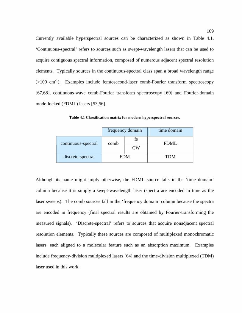
Thermometry in combustion applications by means of laser absorption spectroscopy is a well
established diagnostic. The experimental simplicity and wealth of knowledge that can be
readily gained from an absorption spectrum makes it often times the diagnostic of choice
when interrogating the flow fields of practical combustion devices such as internal
combustion engines.
This project develops techniques for optimizing the design of absorption based sensors by
providing strategies for selecting optimal wavelengths in order to improve thermometry.
Descriptive relations are derived in order to predict the performance of an absorption based
sensor and through numerical optimization, ideal selections of wavelengths can be made.
Furthermore, this work applies novel hyperspectral lasers to practical combustion
environments in order to infer gas properties based on direct absorption spectroscopy. The
measurements are designed for high-speed (30 kHz and up) data rates of useful engineering
parameters such as temperature and species concentration. Measurements have been
performed across the cylinder of an optically accessible HCCI engine using a rapidly-swept
(5 µs measurement time) broad wavelength (1333-1377 nm) tunable laser. Temperature
results were obtained at 100 kHz with 0.25% RMS precision at a temperature of 1970 K.
Page 3
ii
ACKNOWLEDGMENTS
This work would not have been possible without the support and guidance of Professor Scott
Sanders. His ubiquitous enthusiasm for the subject matter is contagious and it provided a
constant source of inspiration
I also would like to express my gratitude towards the rest of my faculty defense committee:
Professors Jaal Ghandhi, Dave Rothamer, John Wright and Claude Woods.
The sheer number of the exceptional people I have been honored to have the opportunity to
work with makes it difficult to name any single one of them and I will be forever indebted to
the many students from the Sanders group and the Engine Research Center for providing me
their valuable time and friendship. However, the insightful discussions over the years with
Laura Kranendonk, Chris Hagen, and Randy Herold have only allowed me to grow both
personally and professionally. I would like to thank Keith Rein for his willingness to drop
everything for a trip to Dayton, Xinliang An for his enthusiasm in taking data at all hours of
the night, and Thilo Kraetschmer for too many reasons to elaborate.
My time at the university would not have been possible without the love and support of my
parents and I will be forever grateful for the opportunities they’ve given me.
Finally, I would like to thank my wife, Tarina, for her unwavering support, friendship, and
love.
Page 4
iii
TABLE OF CONTENTS
Abstract..................................................................................................................................... i Acknowledgments ................................................................................................................... ii Table of Contents ................................................................................................................... iii Table of Figures....................................................................................................................... v List of Tables ......................................................................................................................... xv Introduction............................................................................................................................. 1
1.1 Motivation.................................................................................................................. 2 1.2 Thesis overview ......................................................................................................... 3
Chapter 2. H2O absorption thermometry............................................................................. 5 2.1 H2O spectroscopy for sensor applications ................................................................. 6 2.2 Spectral databases ...................................................................................................... 7
2.2.1 HITRAN ................................................................................................... 8 2.2.2 BT2 ........................................................................................................... 8 2.2.3 Comparing the databases .......................................................................... 9
2.3 Two color ratiometric thermometry......................................................................... 14 2.4 Hyperspectral thermometry ..................................................................................... 17
2.4.1 Linear system of equations ..................................................................... 17 2.4.2 Spectral fitting......................................................................................... 18
Chapter 3. Wavelength selection ........................................................................................ 22 3.1 Introduction.............................................................................................................. 22 3.2 Setup ........................................................................................................................ 24 3.3 Ideal Diatomic Molecule (IDM) model ................................................................... 25
3.3.1 Case 1: 2 wavelengths, known temperature............................................ 27 3.3.2 Case 2: 2 wavelengths, unknown temperature........................................ 38 3.3.3 Case 3: N wavelengths, known temperature........................................... 41 3.3.4 Case 4: N wavelengths, unknown temperature....................................... 50
3.4 H2O Spectrum ......................................................................................................... 58 3.4.1 Case 1: N wavelengths, known temperature........................................... 64 3.4.2 Case 2: N wavelengths, unknown temperature....................................... 69
3.5 Practical techniques for wavelength selection ......................................................... 79 3.5.1 Ratio spectrum ........................................................................................ 81 3.5.2 Difference spectrum................................................................................ 83 3.5.3 Continuous wavelength scan................................................................... 86
Chapter 4. Applications........................................................................................................ 90 4.1 HCCI engine ............................................................................................................ 90
4.1.1 Sensor theory .......................................................................................... 93
Page 5
iv
4.1.2 Noise considerations ............................................................................... 94 4.1.3 Experimental arrangement ...................................................................... 95 4.1.4 Results..................................................................................................... 98 4.1.5 Discussion............................................................................................. 105 4.1.6 Conclusions........................................................................................... 106
4.2 Gas turbine combustor ........................................................................................... 107 4.2.1 Spectral selection and management ...................................................... 112 4.2.2 Experimental arrangement .................................................................... 118 4.2.3 Results and discussion ..........................................................................125 4.2.4 Conclusions........................................................................................... 130
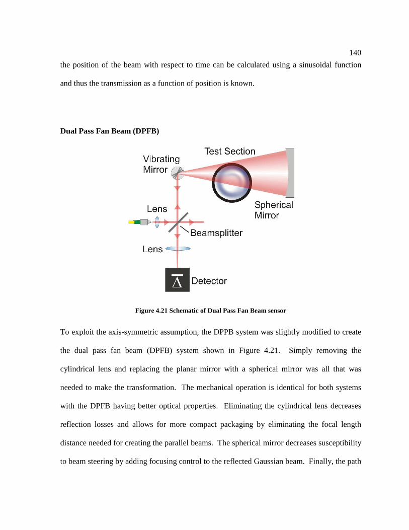
4.3 Rocket plume ......................................................................................................... 130 4.3.1 Management of non-uniform flows ...................................................... 132 4.3.2 Sensor configurations............................................................................ 137 4.3.3 Experimental results.............................................................................. 141
Chapter 5. Conclusions....................................................................................................... 146 5.1 Future work............................................................................................................ 148
References............................................................................................................................ 150
Page 6
v
TABLE OF FIGURES
Figure 2.1 Shown are the normalized line intensities versus rotational quantum number J
for the R branch of the ν1+ν3 band of water (~1330-1370 nm) for the HITRAN
(left) and BT2 (right) databases. The exclusion of high rotational energy lines
is evident in the HITRAN data versus the completeness of the BT2 database. .... 11
Figure 2.2 Subset of spectrum recorded in HCCI piston engine at top dead center (TDC).
The cylinder pressure was 31.8 bar and the absorption path length 9.5 cm.
Plotted against the experimental spectrum are simulations using multiple
databases: HITEMP, HITRAN, and BT2. The HITEMP and HITRAN
simulations are at 1500 K which was the inferred temperature from fitting to
the HITEMP library. The BT2 simulations show improved agreement at 1500
K and even better agreement at 2200 K. ............................................................... 12
Figure 2.3 Temperatures inferred from infrared water vapor absorption versus
temperatures calculated from gas sampling. The cold bias is readily seen in
the HITEMP results whereas the BT2 data more closely follows the ideal trend
line. ........................................................................................................................ 13
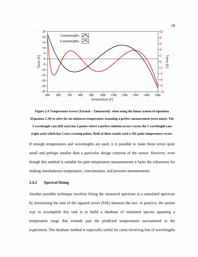
Figure 2.4 Temperature errors (Tactual – Tmeasured) when using the linear system of
equations (Equation 2.10) to solve for an unknown temperature assuming a
perfect measurement (zero noise). The 3 wavelength case (left axis) has 3
points where a perfect solution occurs versus the 5 wavelength case (right
axis) which has 5 zero crossing points. Both of these results used a 101 point
temperature vector. ................................................................................................ 18
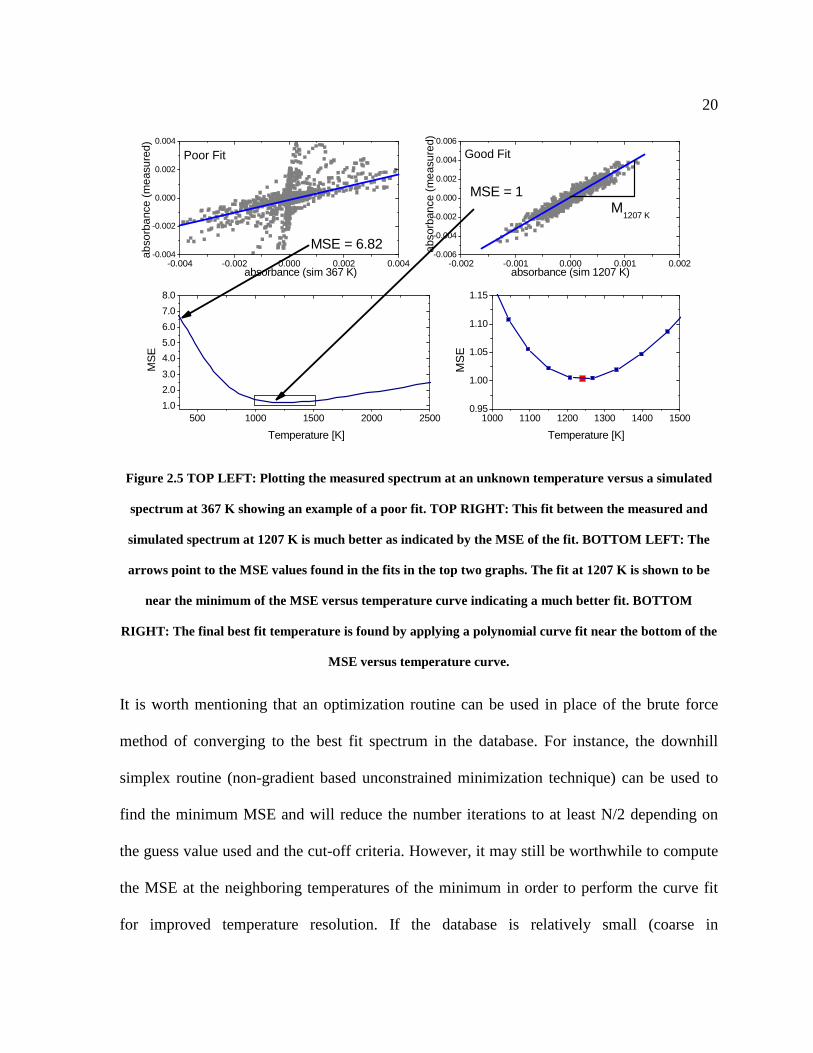
Figure 2.5 TOP LEFT: Plotting the measured spectrum at an unknown temperature
versus a simulated spectrum at 367 K showing an example of a poor fit. TOP
RIGHT: This fit between the measured and simulated spectrum at 1207 K is
much better as indicated by the MSE of the fit. BOTTOM LEFT: The arrows
point to the MSE values found in the fits in the top two graphs. The fit at 1207
K is shown to be near the minimum of the MSE versus temperature curve
Page 7
vi
indicating a much better fit. BOTTOM RIGHT: The final best fit temperature
is found by applying a polynomial curve fit near the bottom of the MSE versus
temperature curve. ................................................................................................. 20
Figure 3.1 Two simulated “absorption” curves of the ideal diatomic model at
temperatures of 500 and 1500 K. The absorption spectrum is simulated by
using the fractional population in each energy level or “J state” and assuming
the total number density, N, is constant at all temperatures. The effect of
temperature is readily seen as an overall decrease in the peak absorbance value
but a larger range of wavelengths having appreciable absorption. ....................... 27
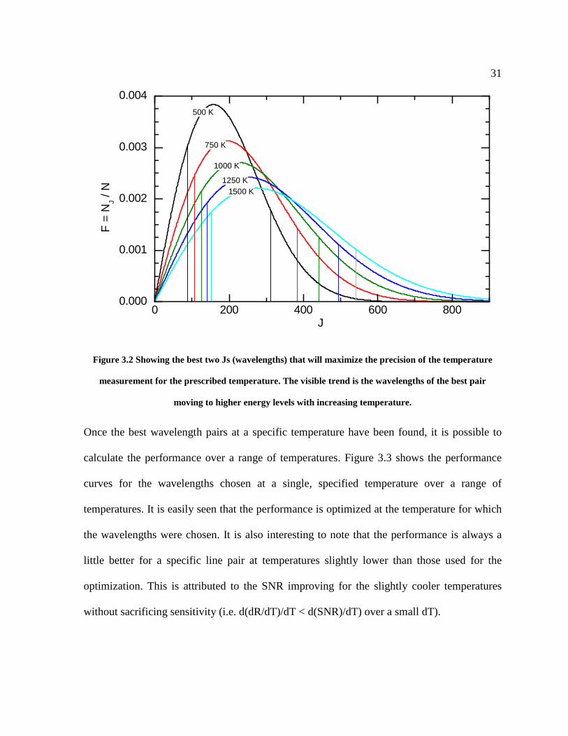
Figure 3.2 Showing the best two Js (wavelengths) that will maximize the precision of the
temperature measurement for the prescribed temperature. The visible trend is
the wavelengths of the best pair moving to higher energy levels with
increasing temperature. ......................................................................................... 31
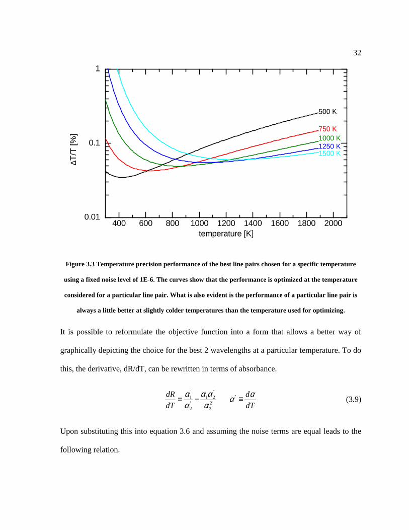
Figure 3.3 Temperature precision performance of the best line pairs chosen for a specific
temperature using a fixed noise level of 1E-6. The curves show that the
performance is optimized at the temperature considered for a particular line
pair. What is also evident is the performance of a particular line pair is always
a little better at slightly colder temperatures than the temperature used for
optimizing.............................................................................................................. 32
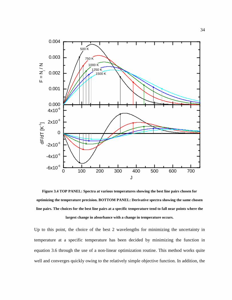
Figure 3.4 TOP PANEL: Spectra at various temperatures showing the best line pairs
chosen for optimizing the temperature precision. BOTTOM PANEL:
Derivative spectra showing the same chosen line pairs. The choices for the
best line pairs at a specific temperature tend to fall near points where the
largest change in absorbance with a change in temperature occurs. ..................... 34
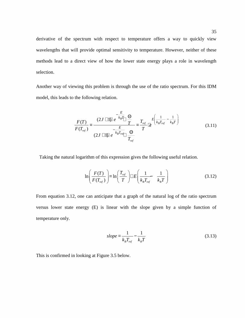
Figure 3.5 Linear relationship between the lower state energy E and the natural log of the
ratio of spectra computed at T and a reference T. The slope is determined by a
simple function of temperature only. .................................................................... 36
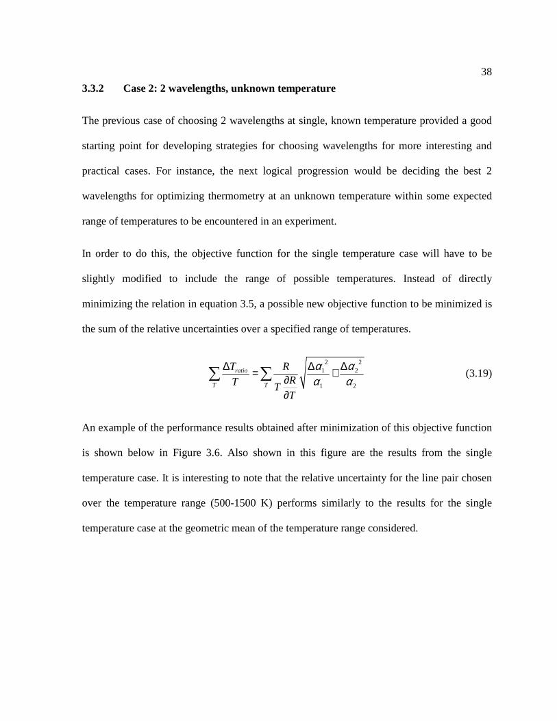
Figure 3.6 Relative uncertainty in temperature versus temperature for the 2 wavelength
case. The result for the best line pair when considering the range of
Page 8
vii
temperatures (500-1500 K) is shown along with the results obtained when
considering a single temperature. .......................................................................... 39
Figure 3.7 The line pair chosen to optimize the relative uncertainty over a range of
temperatures is plotted along with the line pairs chosen for the single
temperature cases. The choice of the best line pair does not correspond to the
best pair at any single temperature. ....................................................................... 40
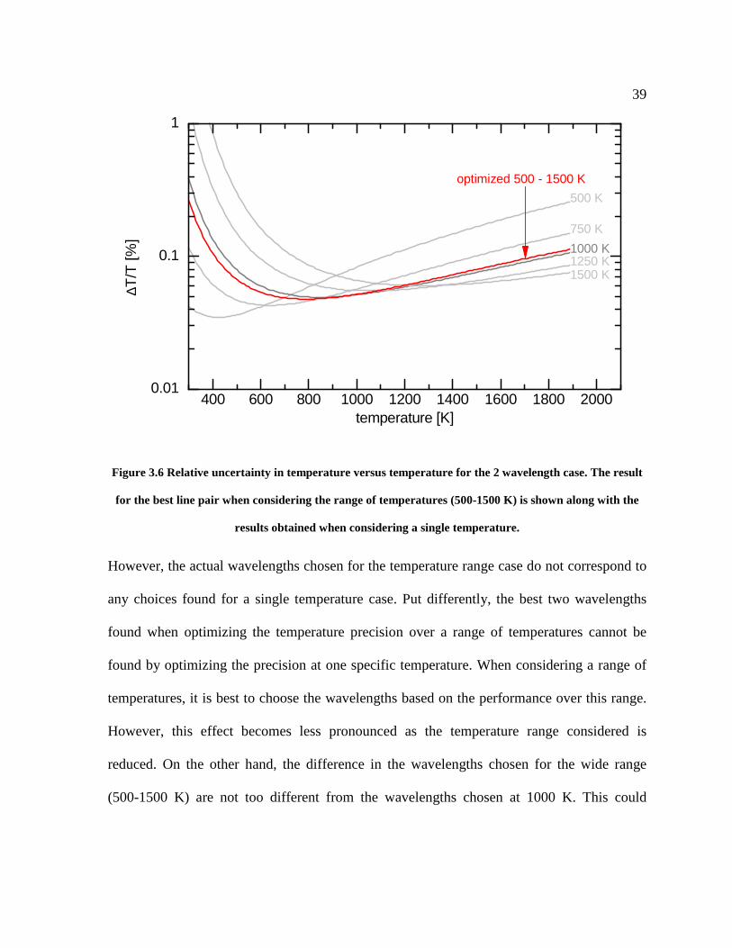
Figure 3.8 Relative uncertainty performance results for the N wavelength case when
optimizing at a single temperature (500 K). The 2 wavelength case is also
shown with the results obtained both through fitting and through the ratio
function derived earlier and good agreement is found between the two. At
fixed performance (i.e. same noise level assumed for all number of
wavelengths) adding wavelengths improves the fidelity of the measurement. ..... 43
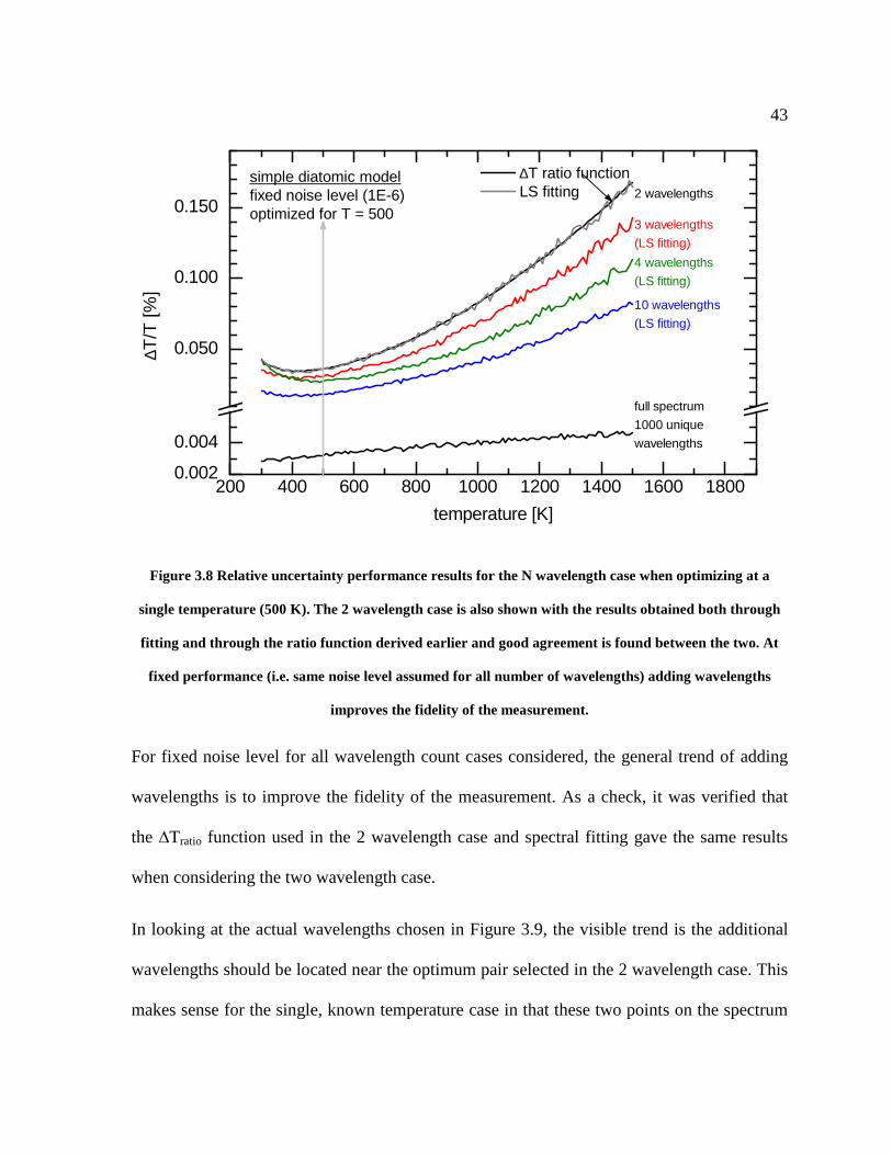
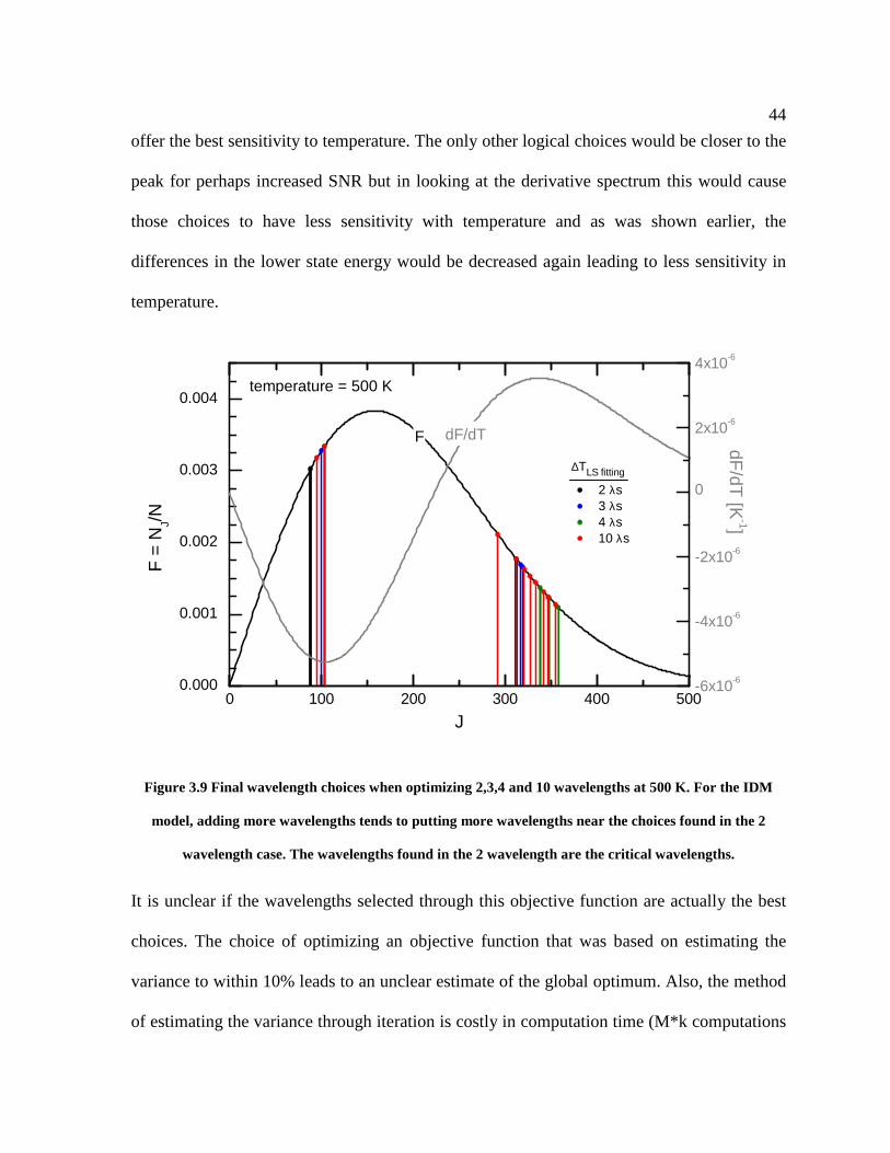
Figure 3.9 Final wavelength choices when optimizing 2,3,4 and 10 wavelengths at 500 K.
For the IDM model, adding more wavelengths tends to putting more
wavelengths near the choices found in the 2 wavelength case. The
wavelengths found in the 2 wavelength are the critical wavelengths. .................. 44
Figure 3.10 Comparison of the results of the N wavelength, single temperature case using
the iLS objective function and the ∆TuwLS objective function. For 2
wavelengths, these two objective functions give the same results and are both
equal to the results given using the ∆Tratio function. However, as N is increased
from 2, the two methods diverge with the ∆TuwLS function leading to a
selection of wavelengths with better performance. ............................................... 48
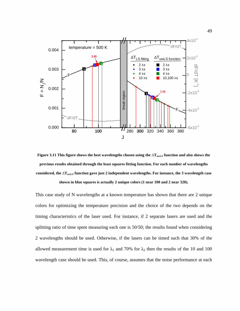
Figure 3.11 This figure shows the best wavelengths chosen using the ∆TuwLS function and
also shows the previous results obtained through the least squares fitting
function. For each number of wavelengths considered, the ∆TuwLS function
gave just 2 independent wavelengths. For instance, the 3 wavelength case
shown in blue squares is actually 2 unique colors (1 near 100 and 2 near 320). .. 49
Page 9
viii
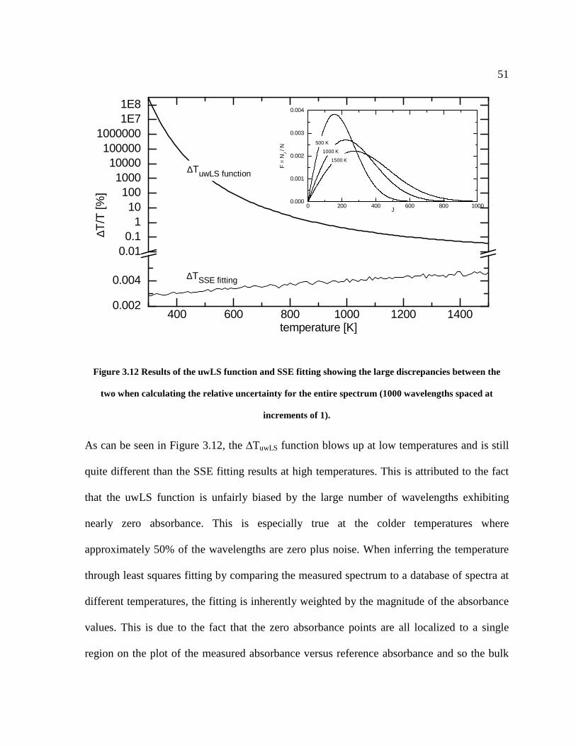
Figure 3.12 Results of the uwLS function and SSE fitting showing the large discrepancies
between the two when calculating the relative uncertainty for the entire
spectrum (1000 wavelengths spaced at increments of 1). ..................................... 51
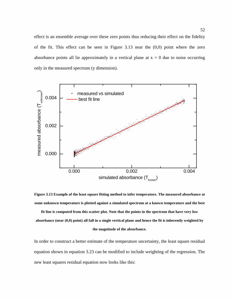
Figure 3.13 Example of the least square fitting method to infer temperature. The
measured absorbance at some unknown temperature is plotted against a
simulated spectrum at a known temperature and the best fit line is computed
from this scatter plot. Note that the points in the spectrum that have very low
absorbance (near (0,0) point) all fall in a single vertical plane and hence the fit
is inherently weighted by the magnitude of the absorbance. ................................ 52
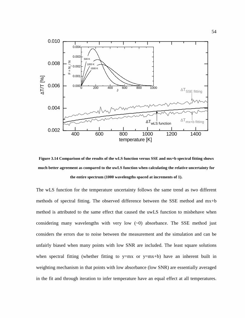
Figure 3.14 Comparison of the results of the wLS function versus SSE and mx+b spectral
fitting shows much better agreement as compared to the uwLS function when
calculating the relative uncertainty for the entire spectrum (1000 wavelengths
spaced at increments of 1). .................................................................................... 54
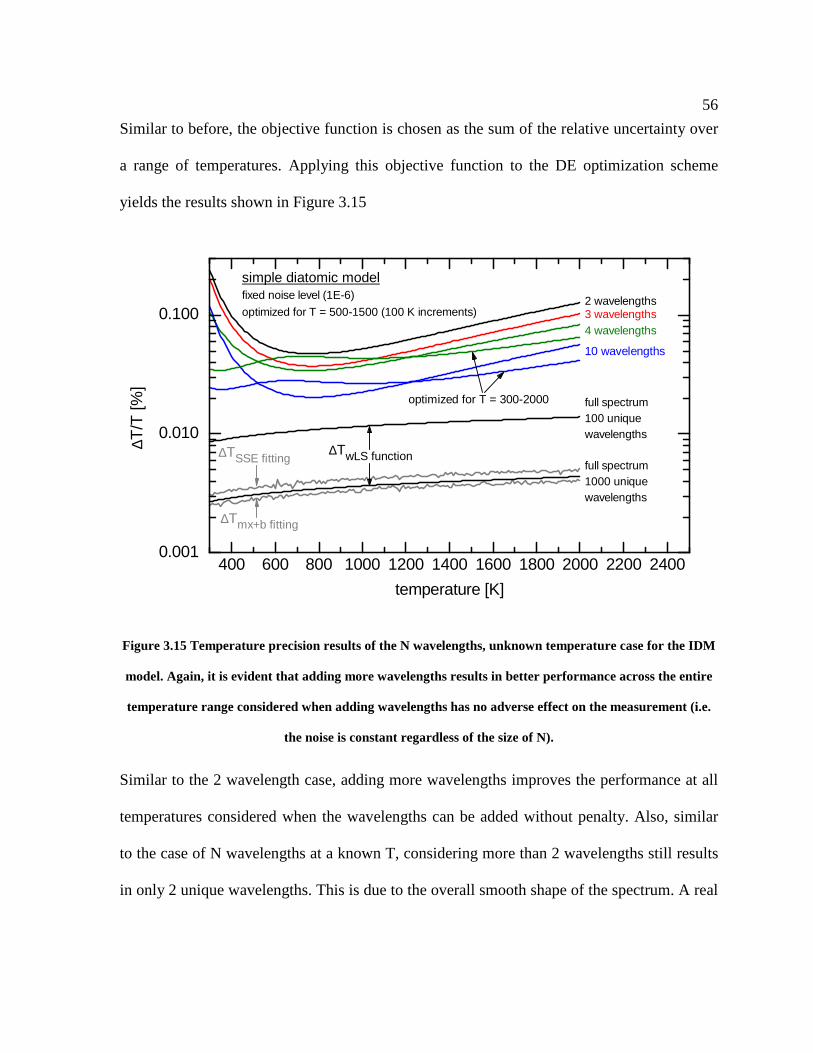
Figure 3.15 Temperature precision results of the N wavelengths, unknown temperature
case for the IDM model. Again, it is evident that adding more wavelengths
results in better performance across the entire temperature range considered
when adding wavelengths has no adverse effect on the measurement (i.e. the
noise is constant regardless of the size of N). .......................................................56
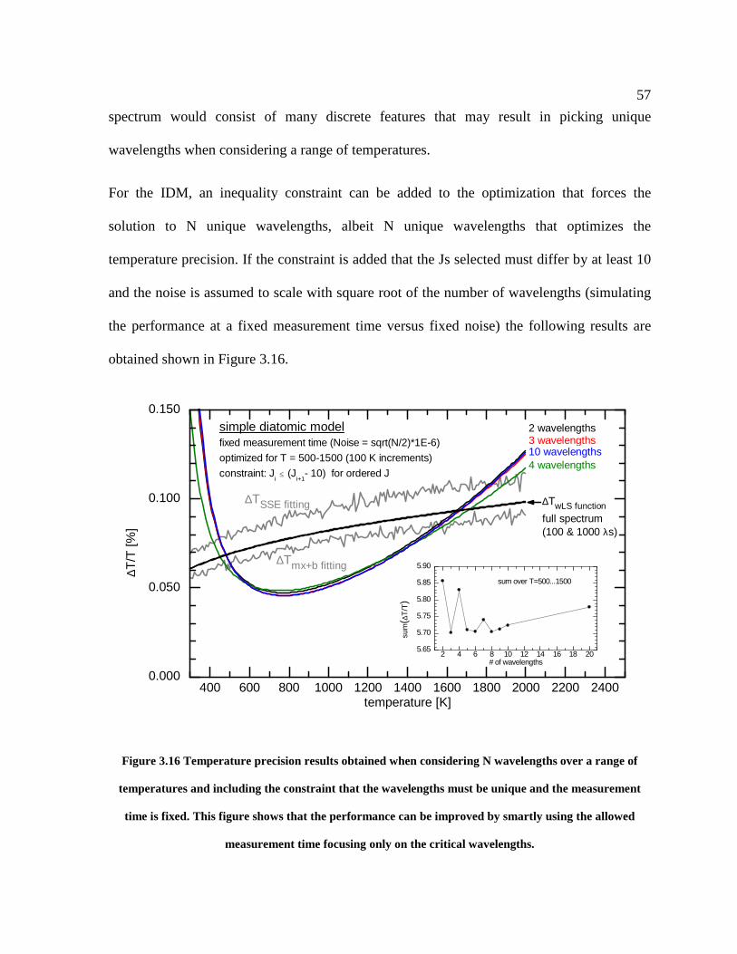
Figure 3.16 Temperature precision results obtained when considering N wavelengths
over a range of temperatures and including the constraint that the wavelengths
must be unique and the measurement time is fixed. This figure shows that the
performance can be improved by smartly using the allowed measurement time
focusing only on the critical wavelengths. ............................................................57
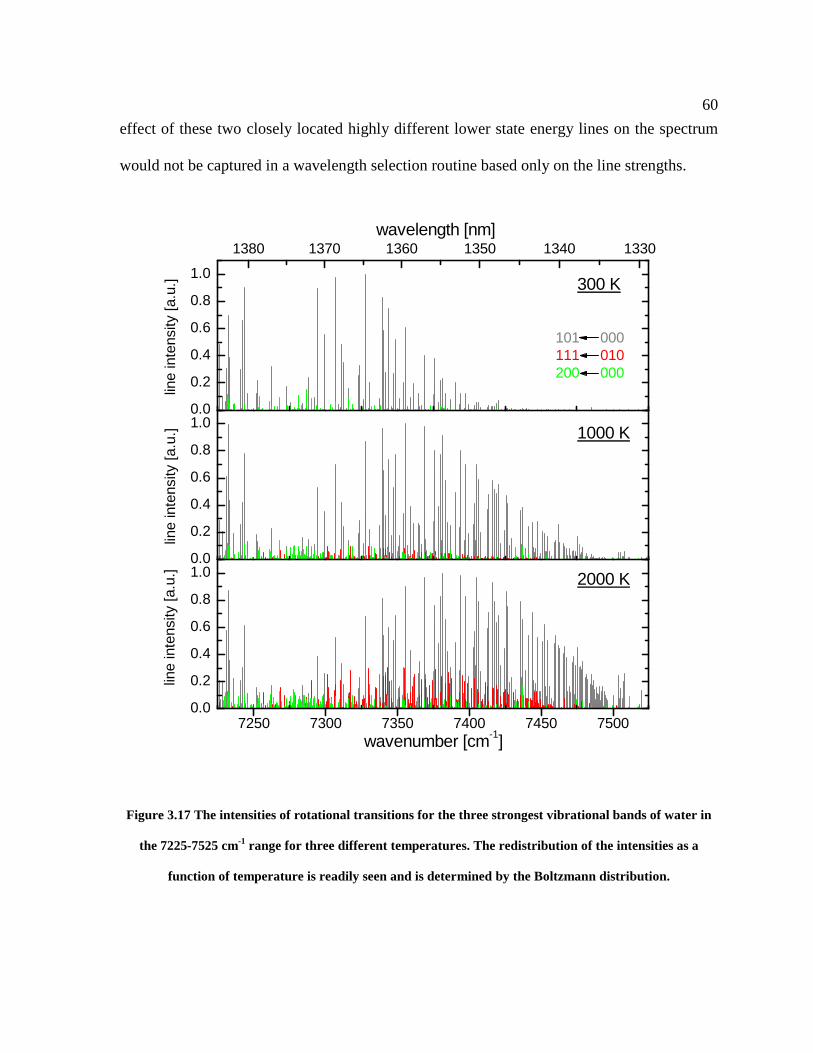
Figure 3.17 The intensities of rotational transitions for the three strongest vibrational
bands of water in the 7225-7525 cm-1 range for three different temperatures.
The redistribution of the intensities as a function of temperature is readily seen
and is determined by the Boltzmann distribution.................................................. 60
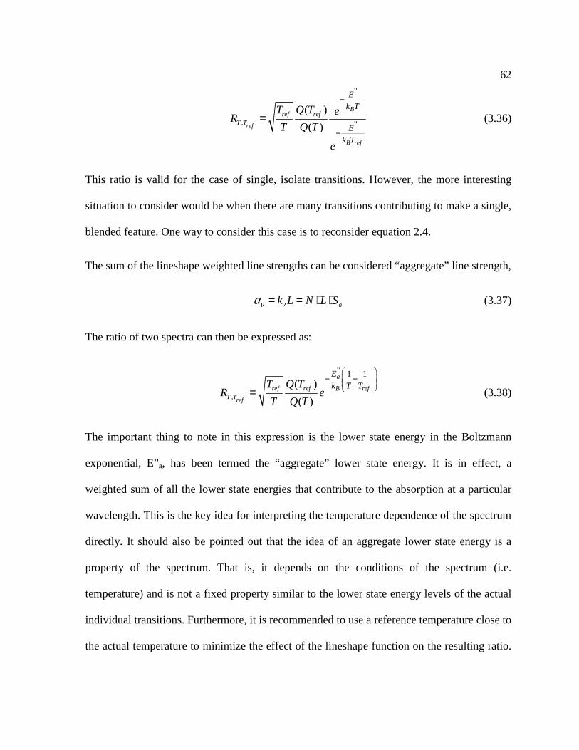
Figure 3.18 The water spectrum shows the same linear relationship as the IDM when
plotting the natural log of the ratio of the spectrum to a spectrum at a reference
Page 10
ix
temperature versus an aggregate lower state energy. The slope of these curves
has the same simple dependence on temperature as the curves in the IDM. ........ 64
Figure 3.19 BOTTOM PANEL: Overlaid on the spectrum is the best wavelength choices
for 2, 3, 4, and 10 wavelengths at a temperature of 313 K with these choices
represented by the sized and colored points (2 – black, smallest….10 – blue,
largest). TOP PANEL: The aggregate lower state energy for this spectrum
showing the best 10 wavelengths. ......................................................................... 66
Figure 3.20 BOTTOM PANEL: Overlaid on the spectrum is the best wavelength choices
for 2, 3, 4, and 10 wavelengths at a temperature of 1008 K with these choices
represented by the sized and colored points (2 – black, smallest….10 – blue,
largest). TOP PANEL: The aggregate lower state energy for this spectrum
showing the best 10 wavelengths. ......................................................................... 67
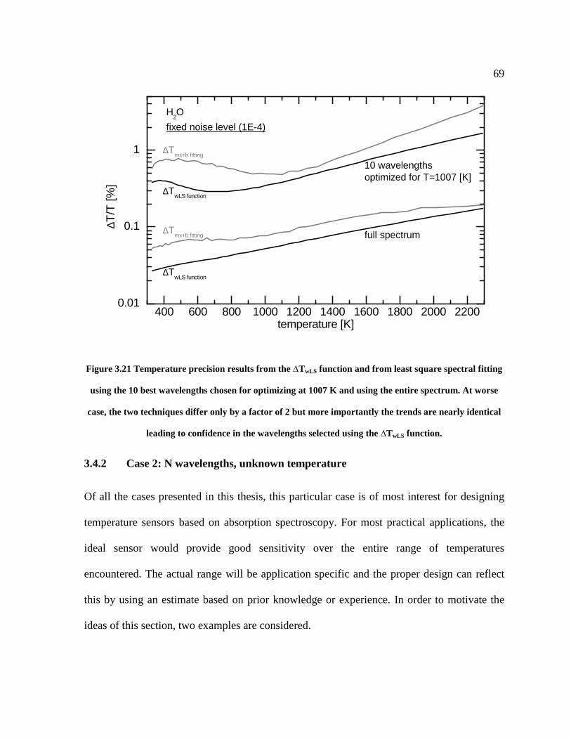
Figure 3.21 Temperature precision results from the ∆TwLS function and from least square
spectral fitting using the 10 best wavelengths chosen for optimizing at 1007 K
and using the entire spectrum. At worse case, the two techniques differ only
by a factor of 2 but more importantly the trends are nearly identical leading to
confidence in the wavelengths selected using the ∆TwLS function........................ 69
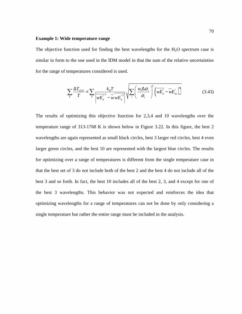
Figure 3.22 BOTTOM PANEL: Overlaid on the spectrum at 1768 K is the best
wavelength choices for 2, 3, 4, and 10 wavelengths optimized over the
temperature range of 313 – 1768 K with these choices represented by the sized
and colored points (2 – black, smallest….10 – blue, largest). TOP PANEL:
The aggregate lower state energy for this spectrum showing the best 10
wavelengths. .......................................................................................................... 71
Figure 3.23 Relative uncertainty of best 2, 3, 4, 10, and 25 wavelengths for the H2O
spectrum when considering a wide range of temperatures. Also shown are the
results when using the entire spectrum. For a fixed noise level, the
performance improves with increasing number of wavelengths........................... 72
Page 11
x
Figure 3.24 The relative uncertainties of the same wavelengths shown above but
considering a fixed measurement time where wavelengths are added at the
expense of increased noise in the measurement. ................................................... 73
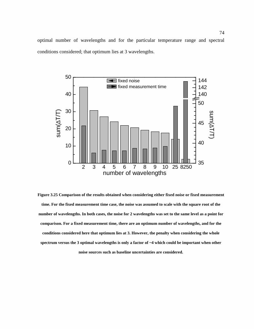
Figure 3.25 Comparison of the results obtained when considering either fixed noise or
fixed measurement time. For the fixed measurement time case, the noise was
assumed to scale with the square root of the number of wavelengths. In both
cases, the noise for 2 wavelengths was set to the same level as a point for
comparison. For a fixed measurement time, there are an optimum number of
wavelengths, and for the conditions considered here that optimum lies at 3.
However, the penalty when considering the whole spectrum versus the 3
optimal wavelengths is only a factor of ~4 which could be important when
other noise sources such as baseline uncertainties are considered. ....................... 74
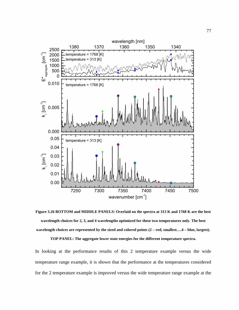
Figure 3.26 BOTTOM and MIDDLE PANELS: Overlaid on the spectra at 313 K and
1768 K are the best wavelength choices for 2, 3, and 4 wavelengths optimized
for these two temperatures only. The best wavelength choices are represented
by the sized and colored points (2 – red, smallest….4 – blue, largest). TOP
PANEL: The aggregate lower state energies for the different temperature
spectra.................................................................................................................... 77
Figure 3.27 Comparing the temperature precision results of the wide temperature range
and the two widely separated temperatures examples. The effect of not
including the intermediate temperatures is easily visible in the 2 temperature
case with a decrease in the precision at intermediate temperatures. However,
the two temperature case does improve the performance at the temperatures
considered versus the wide temperature range optimization................................. 78
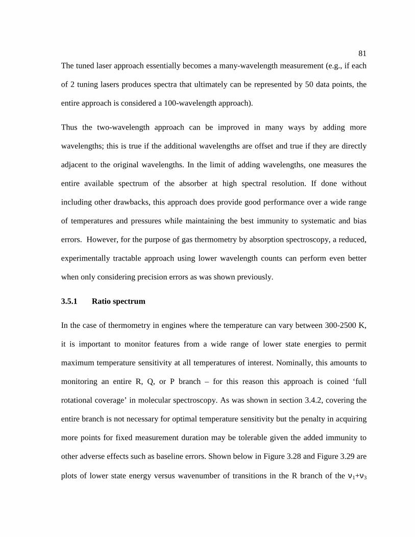
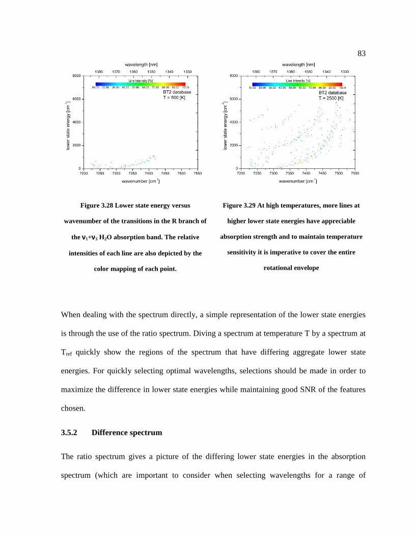
Figure 3.28 Lower state energy versus wavenumber of the transitions in the R branch of
the ν1+ν3 H2O absorption band. The relative intensities of each line are also
depicted by the color mapping of each point. ....................................................... 83
Page 12
xi
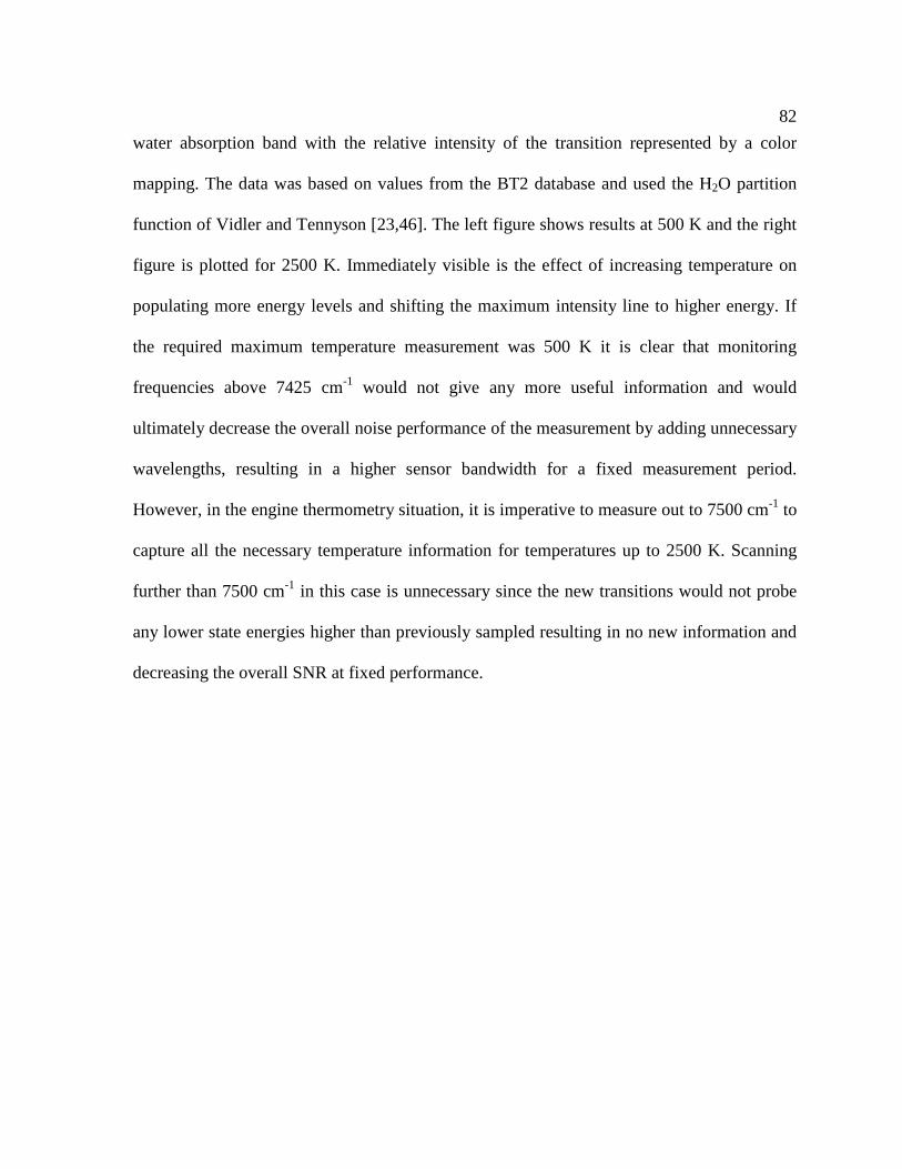
Figure 3.29 At high temperatures, more lines at higher lower state energies have
appreciable absorption strength and to maintain temperature sensitivity it is
imperative to cover the entire rotational envelope ................................................ 83
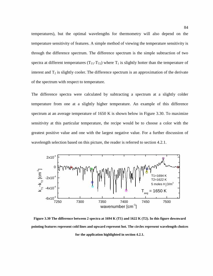
Figure 3.30 The difference between 2 spectra at 1694 K (T1) and 1622 K (T2). In this
figure downward pointing features represent cold lines and upward represent
hot. The circles represent wavelength choices for the application highlighted
in section 4.2.1....................................................................................................... 84
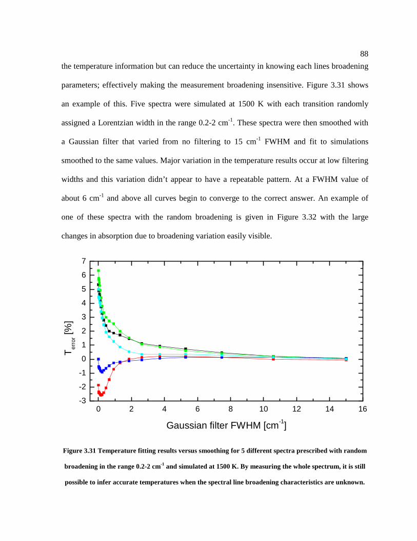
Figure 3.31 Temperature fitting results versus smoothing for 5 different spectra
prescribed with random broadening in the range 0.2-2 cm-1 and simulated at
1500 K. By measuring the whole spectrum, it is still possible to infer accurate
temperatures when the spectral line broadening characteristics are unknown...... 88
Figure 3.32 Spectra showing the difference between constant, low (0.2 cm-1) broadening
and one with variable, random broadening in the range 0.2-2 cm-1. Even with
the large difference in the lineshape function, the temperature information is
retained when measuring the whole spectrum. The width of a scan required is
dependent on the uncertainty in broadening and shown in this figure is a
subset of the whole spectrum considered for inferring the temperature. .............. 89
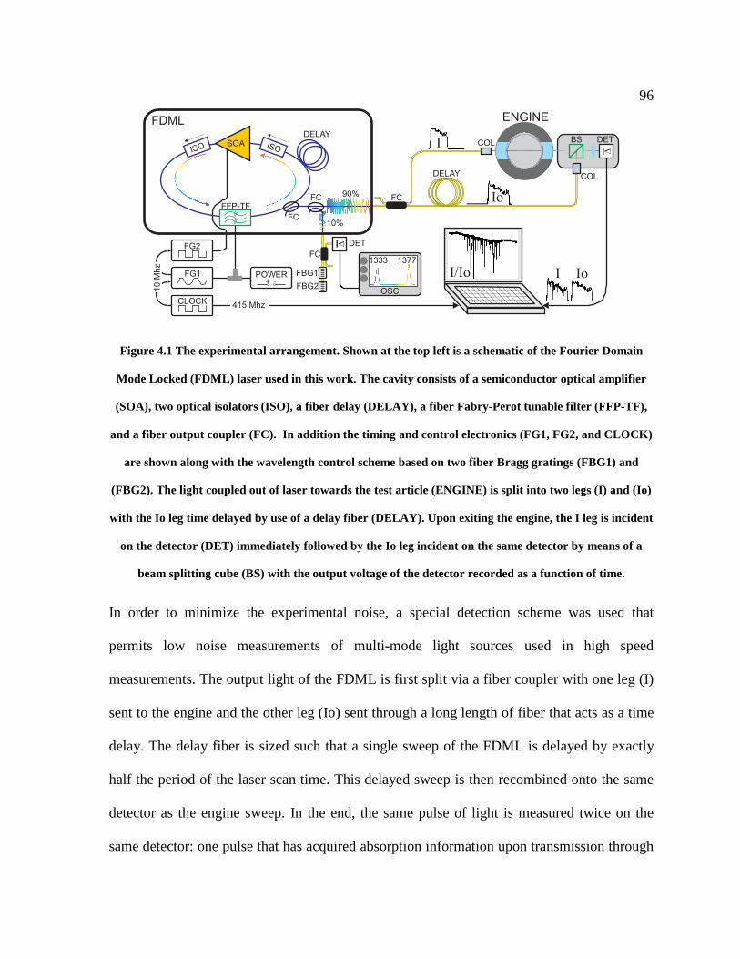
Figure 4.1 The experimental arrangement. Shown at the top left is a schematic of the
Fourier Domain Mode Locked (FDML) laser used in this work. The cavity
consists of a semiconductor optical amplifier (SOA), two optical isolators
(ISO), a fiber delay (DELAY), a fiber Fabry-Perot tunable filter (FFP-TF), and
a fiber output coupler (FC). In addition the timing and control electronics
(FG1, FG2, and CLOCK) are shown along with the wavelength control
scheme based on two fiber Bragg gratings (FBG1) and (FBG2). The light
coupled out of laser towards the test article (ENGINE) is split into two legs (I)
and (Io) with the Io leg time delayed by use of a delay fiber (DELAY). Upon
exiting the engine, the I leg is incident on the detector (DET) immediately
followed by the Io leg incident on the same detector by means of a beam
splitting cube (BS) with the output voltage of the detector recorded as a
function of time. .................................................................................................... 96
Page 13
xii
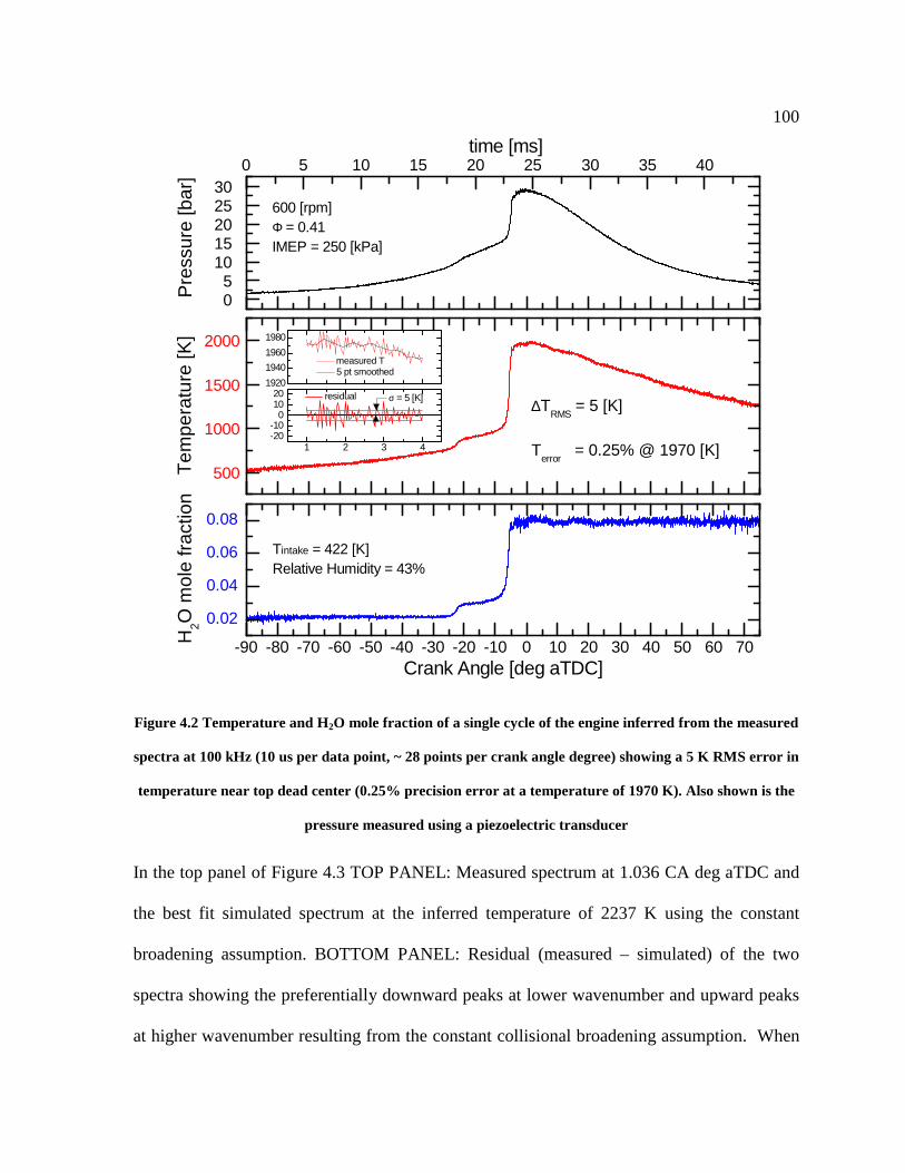
Figure 4.2 Temperature and H2O mole fraction of a single cycle of the engine inferred
from the measured spectra at 100 kHz (10 us per data point, ~ 28 points per
crank angle degree) showing a 5 K RMS error in temperature near top dead
center (0.25% precision error at a temperature of 1970 K). Also shown is the
pressure measured using a piezoelectric transducer............................................ 100
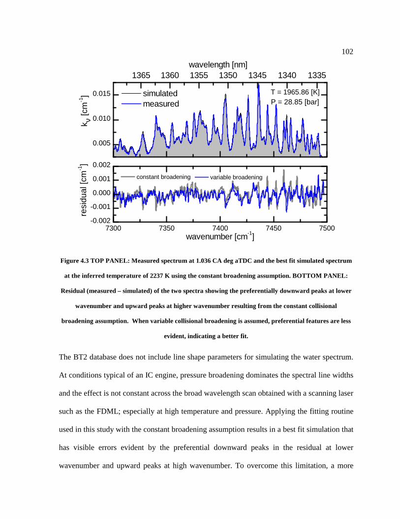
Figure 4.3 TOP PANEL: Measured spectrum at 1.036 CA deg aTDC and the best fit
simulated spectrum at the inferred temperature of 2237 K using the constant
broadening assumption. BOTTOM PANEL: Residual (measured – simulated)
of the two spectra showing the preferentially downward peaks at lower
wavenumber and upward peaks at higher wavenumber resulting from the
constant collisional broadening assumption. When variable collisional
broadening is assumed, preferential features are less evident, indicating a
better fit. .............................................................................................................. 102
Figure 4.4 Difference in temperature and H2O mole fraction results when fitting to
simulations using constant and variable broadening. The variable broadening
scheme led to better agreement based on the mean square error of the
difference between the measured spectrum and the simulated spectrum at the
best fit temperature. Furthermore, the otherwise unexplainable slopes in the
H2O mole fraction curve for the constant broadening case pre and post
combustion is not present when including variable broadening. ........................ 104
Figure 4.5 Comparison of temperature results between the absorption spectroscopy
experiment and simulation based on the KIVA CFD code. The fully 3D results
of the simulation were averaged along the same path the laser beam traversed
and good agreement is found between the two. .................................................. 105
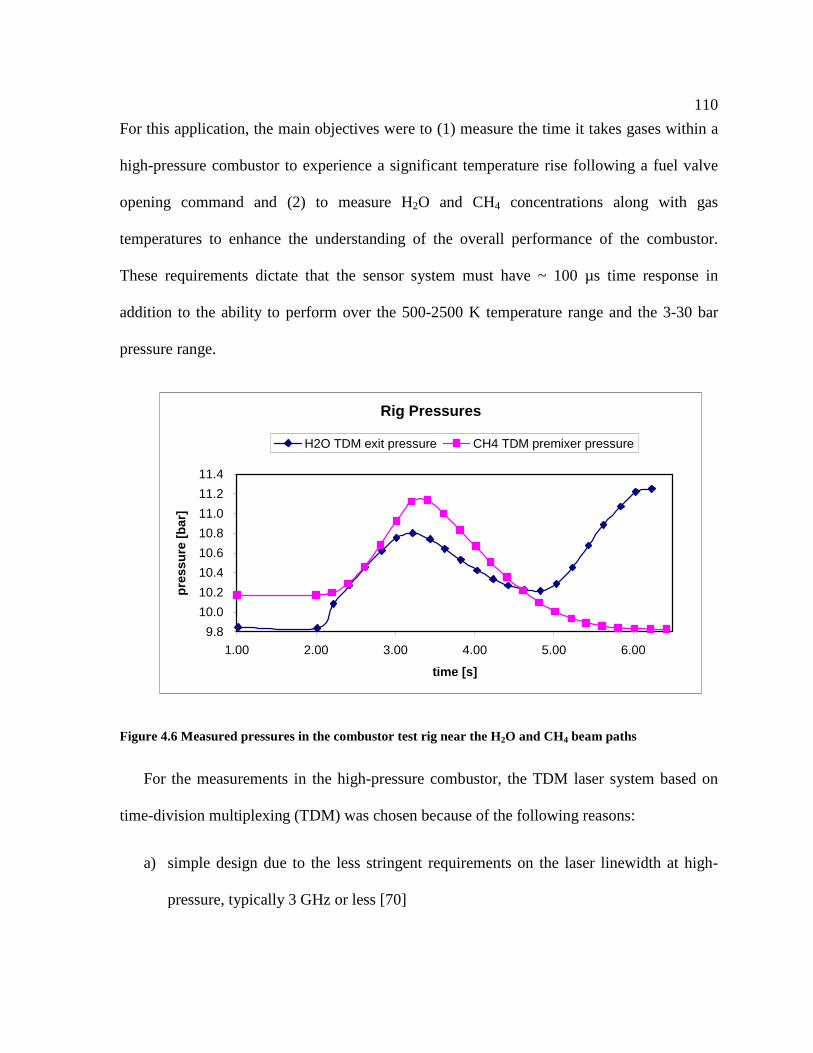
Figure 4.6 Measured pressures in the combustor test rig near the H2O and CH4 beam
paths..................................................................................................................... 110
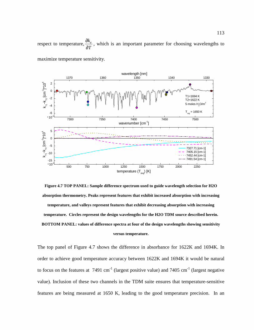
Figure 4.7 TOP PANEL: Sample difference spectrum used to guide wavelength selection
for H2O absorption thermometry. Peaks represent features that exhibit
increased absorption with increasing temperature, and valleys represent
features that exhibit decreasing absorption with increasing temperature.
Page 14
xiii
Circles represent the design wavelengths for the H2O TDM source described
herein. BOTTOM PANEL: values of difference spectra at four of the design
wavelengths showing sensitivity versus temperature.......................................... 113
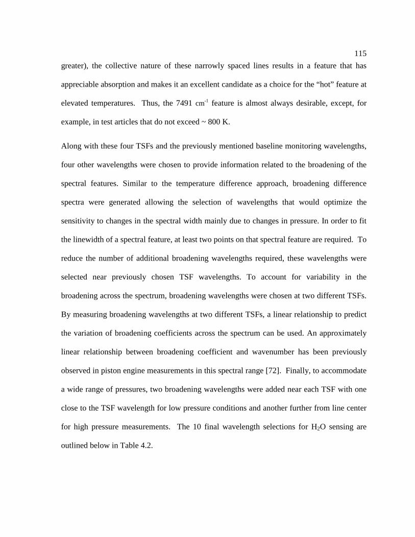
Figure 4.8: Simulated CH4 spectrum showing the four wavelengths chosen for the fuel
TDM laser............................................................................................................ 117
Figure 4.9: Raw single-cycle time trace of the 10-color H2O TDM laser utilizing pulse
delay referencing ................................................................................................. 119
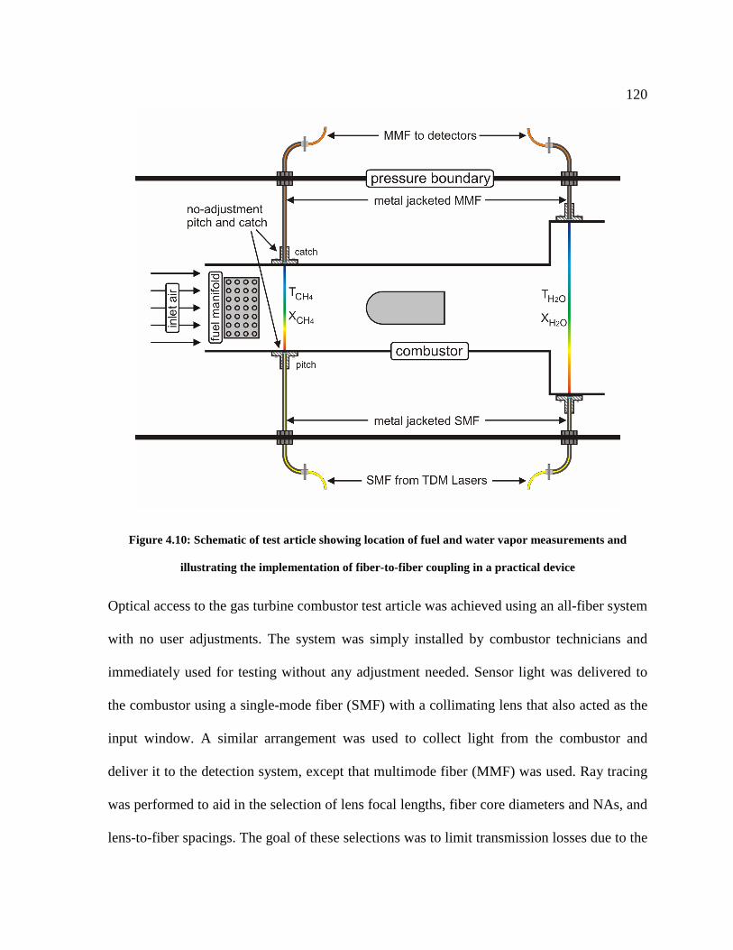
Figure 4.10: Schematic of test article showing location of fuel and water vapor
measurements and illustrating the implementation of fiber-to-fiber coupling in
a practical device ................................................................................................. 120
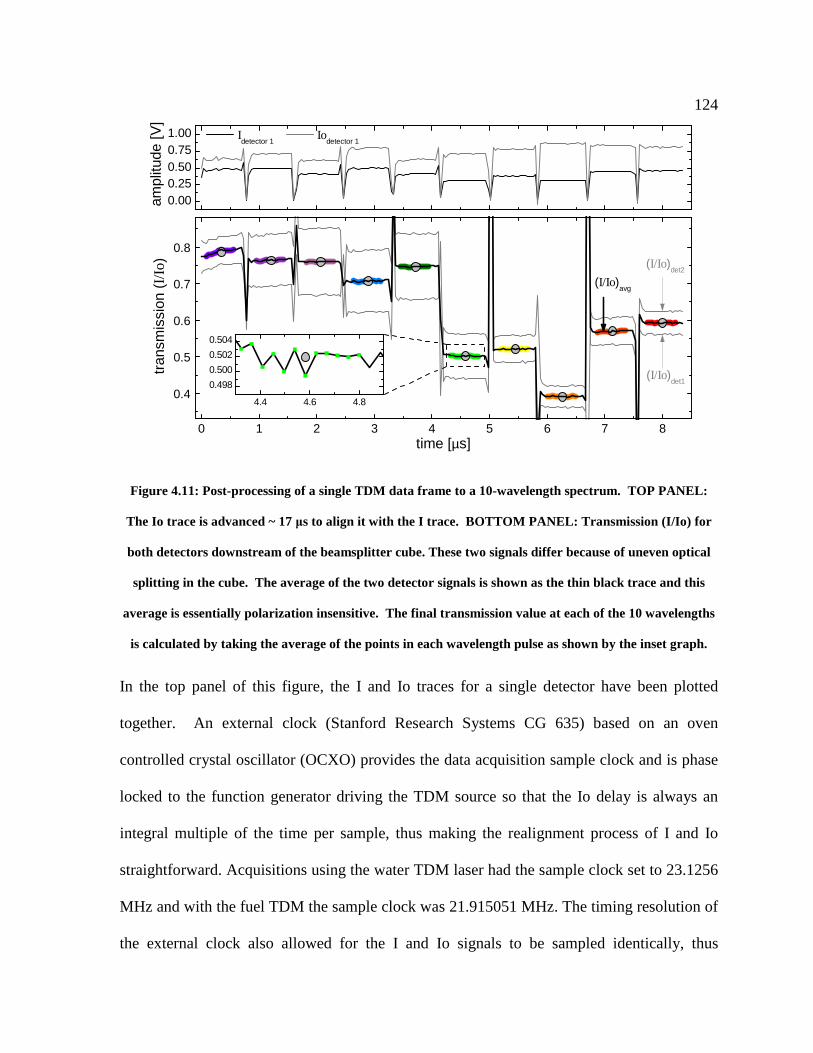
Figure 4.11: Post-processing of a single TDM data frame to a 10-wavelength spectrum.
TOP PANEL: The Io trace is advanced ~ 17 µs to align it with the I trace.
BOTTOM PANEL: Transmission (I/Io) for both detectors downstream of the
beamsplitter cube. These two signals differ because of uneven optical splitting
in the cube. The average of the two detector signals is shown as the thin black
trace and this average is essentially polarization insensitive. The final
transmission value at each of the 10 wavelengths is calculated by taking the
average of the points in each wavelength pulse as shown by the inset graph..... 124
Figure 4.12 CH4 absorbance versus time at the four wavelengths highlighted in the inset
spectrum .............................................................................................................. 126
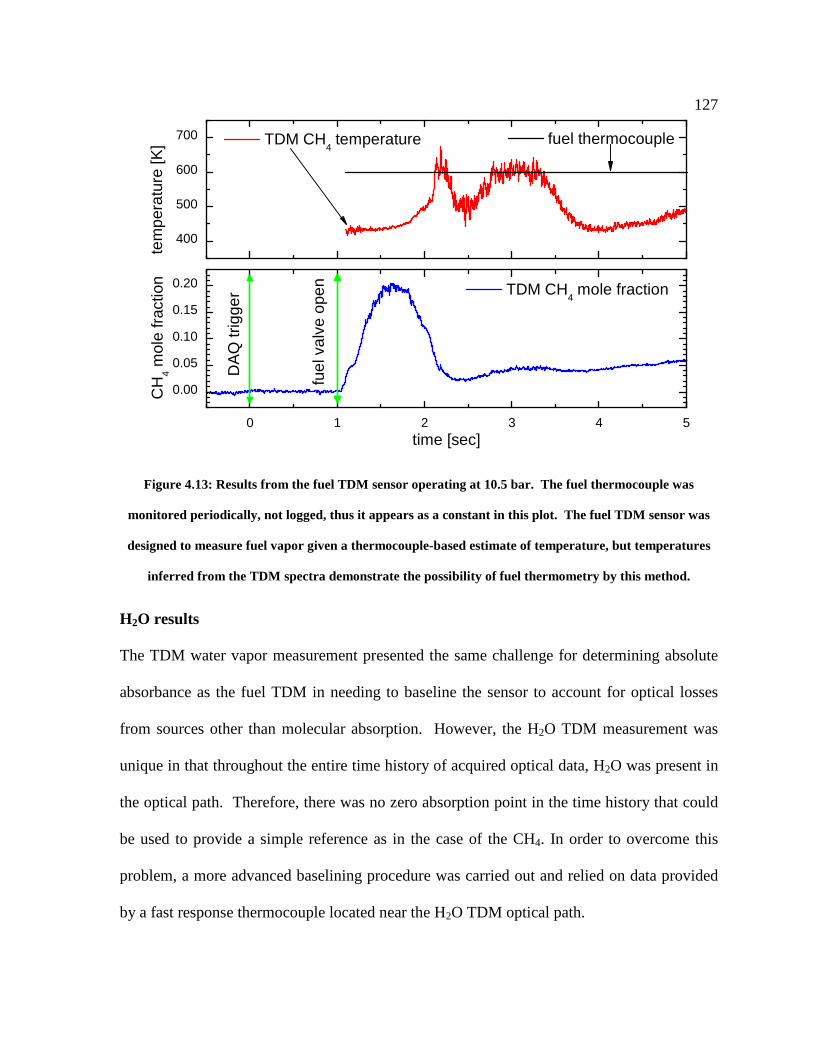
Figure 4.13: Results from the fuel TDM sensor operating at 10.5 bar. The fuel
thermocouple was monitored periodically, not logged, thus it appears as a
constant in this plot. The fuel TDM sensor was designed to measure fuel
vapor given a thermocouple-based estimate of temperature, but temperatures
inferred from the TDM spectra demonstrate the possibility of fuel
thermometry by this method................................................................................ 127
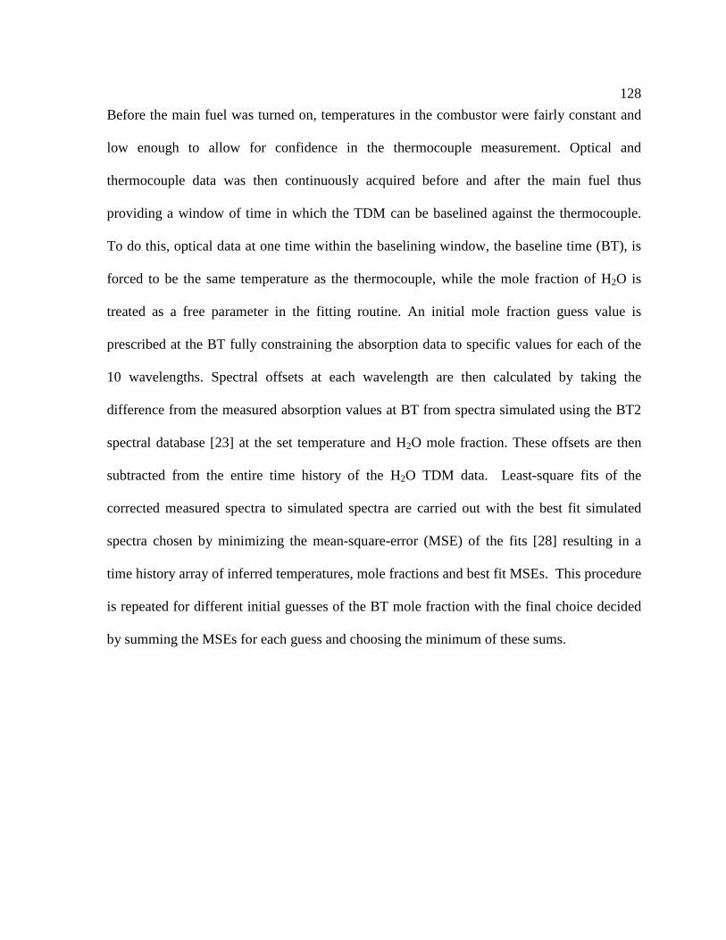
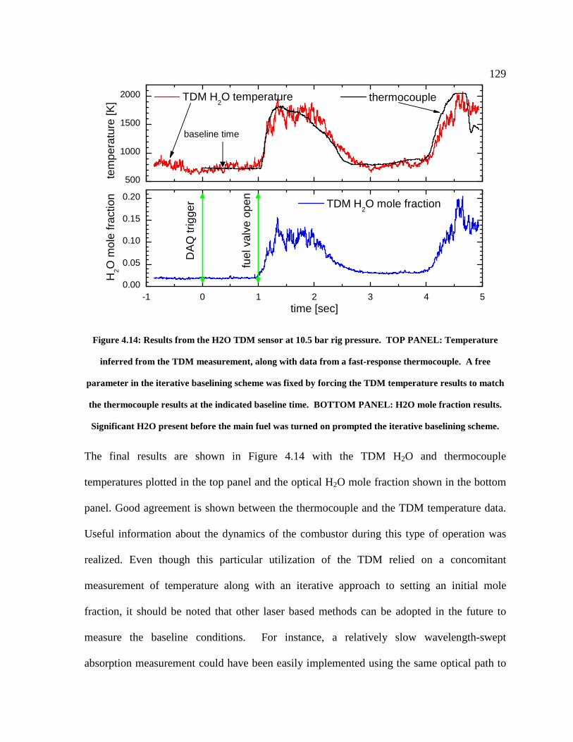
Figure 4.14: Results from the H2O TDM sensor at 10.5 bar rig pressure. TOP PANEL:
Temperature inferred from the TDM measurement, along with data from a
fast-response thermocouple. A free parameter in the iterative baselining
Page 15
xiv
scheme was fixed by forcing the TDM temperature results to match the
thermocouple results at the indicated baseline time. BOTTOM PANEL: H2O
mole fraction results. Significant H2O present before the main fuel was turned
on prompted the iterative baselining scheme. ..................................................... 129
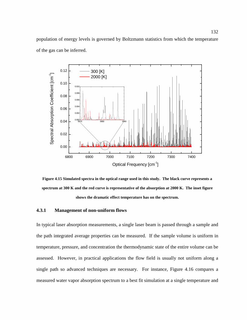
Figure 4.15 Simulated spectra in the optical range used in this study. The black curve
represents a spectrum at 300 K and the red curve is representative of the
absorption at 2000 K. The inset figure shows the dramatic effect temperature
has on the spectrum. ............................................................................................ 132
Figure 4.16 Absorption spectrum along a non-uniform path. The measured spectrum fits
better to a weighted superposition of multiple temperature simulations versus a
single temperature simulation. ............................................................................ 133
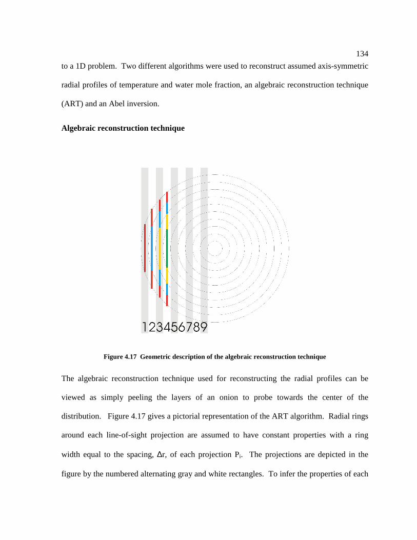
Figure 4.17 Geometric description of the algebraic reconstruction technique .................... 134
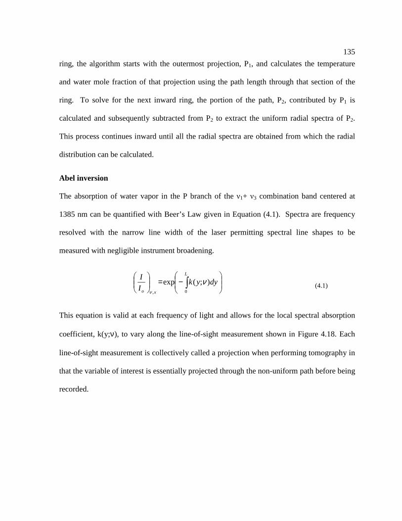
Figure 4.18 Geometric description of variables used in the Abel transform....................... 136
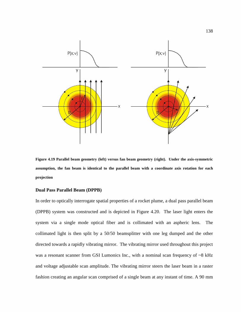
Figure 4.19 Parallel beam geometry (left) versus fan beam geometry (right). Under the
axis-symmetric assumption, the fan beam is identical to the parallel beam with
a coordinate axis rotation for each projection ..................................................... 138
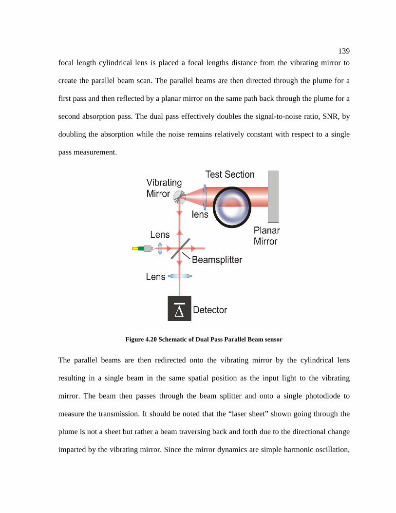
Figure 4.20 Schematic of Dual Pass Parallel Beam sensor .................................................. 139
Figure 4.21 Schematic of Dual Pass Fan Beam sensor......................................................... 140
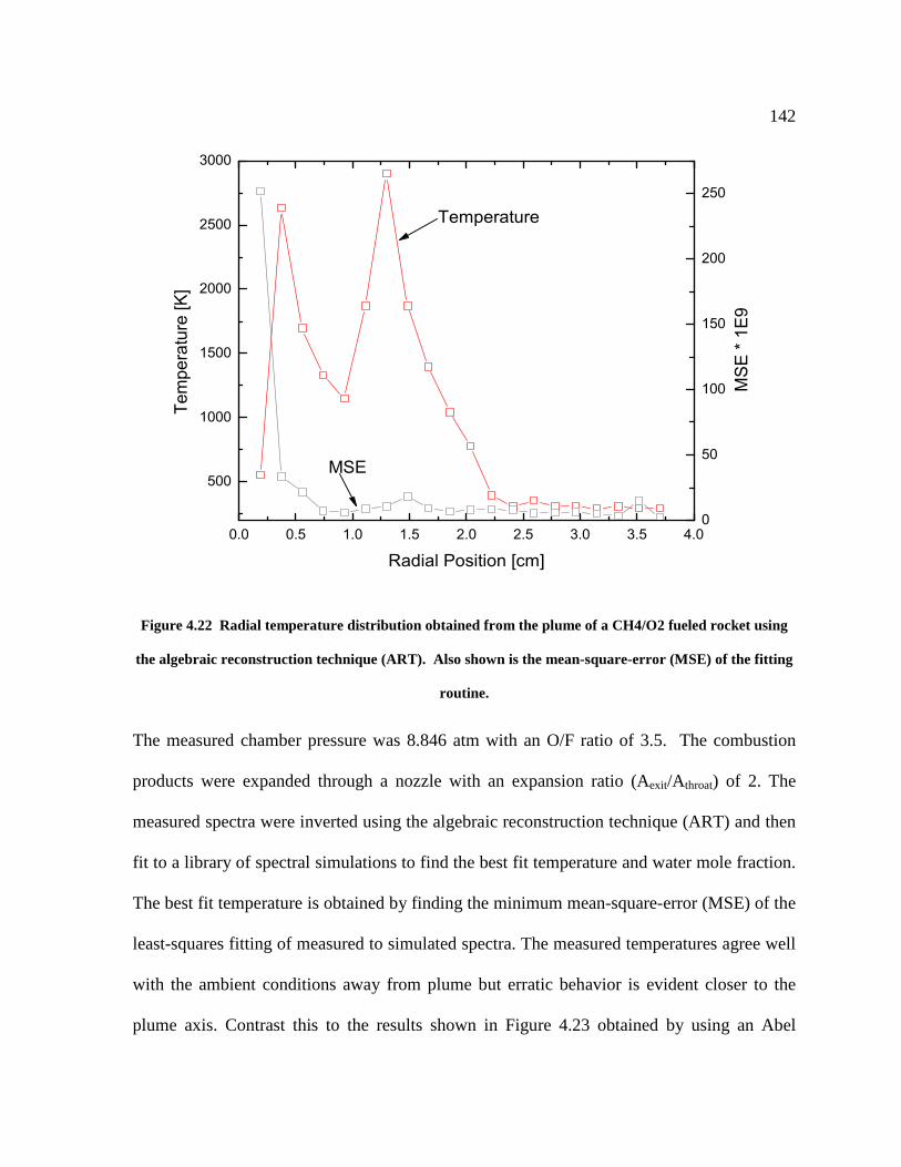
Figure 4.22 Radial temperature distribution obtained from the plume of a CH4/O2 fueled
rocket using the algebraic reconstruction technique (ART). Also shown is the
mean-square-error (MSE) of the fitting routine. ................................................. 142
Figure 4.23 Temperature and water mole fraction radial profiles using an Abel inversion
on the same experimental data used in Figure 4.22. The Abel inversion leads
to better fits to simulations (lower MSE values) resulting in smoother profiles
near the center of the plume. ............................................................................... 143
Figure 4.24 Temperature profile from measurements of the plume gas from two different
rocket motors. Also shown is the calculated temperature from chemical
equilibrium and the length of the CEA calculated lines represents the radius of
the exit of the nozzle. .......................................................................................... 145
Page 16
xv
LIST OF TABLES
Table 4.1 Classification matrix for modern hyperspectral sources....................................... 109
Table 4.2 Wavelengths used in the H2O TDM laser system. Design and actual / measured
wavelengths differ because of imperfect temperature control of the fiber Bragg
gratings. Overall, ten wavelengths were chosen: 4 for monitoring peak
absorbance of temperature-sensitive features, 4 for monitoring feature
broadening (2 are best when the broadening is high and 2 are best when the
broadening is low), and 2 for tracking baseline changes. ................................... 116
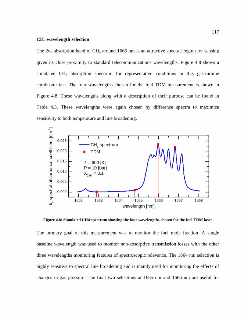
Table 4.3 TDM wavelengths used for the CH4 measurement. In total, 4 wavelengths were
selected: 2 to monitor temperature-sensitive features, 1 for line broadening,
and 1 for tracking baseline errors. ....................................................................... 118
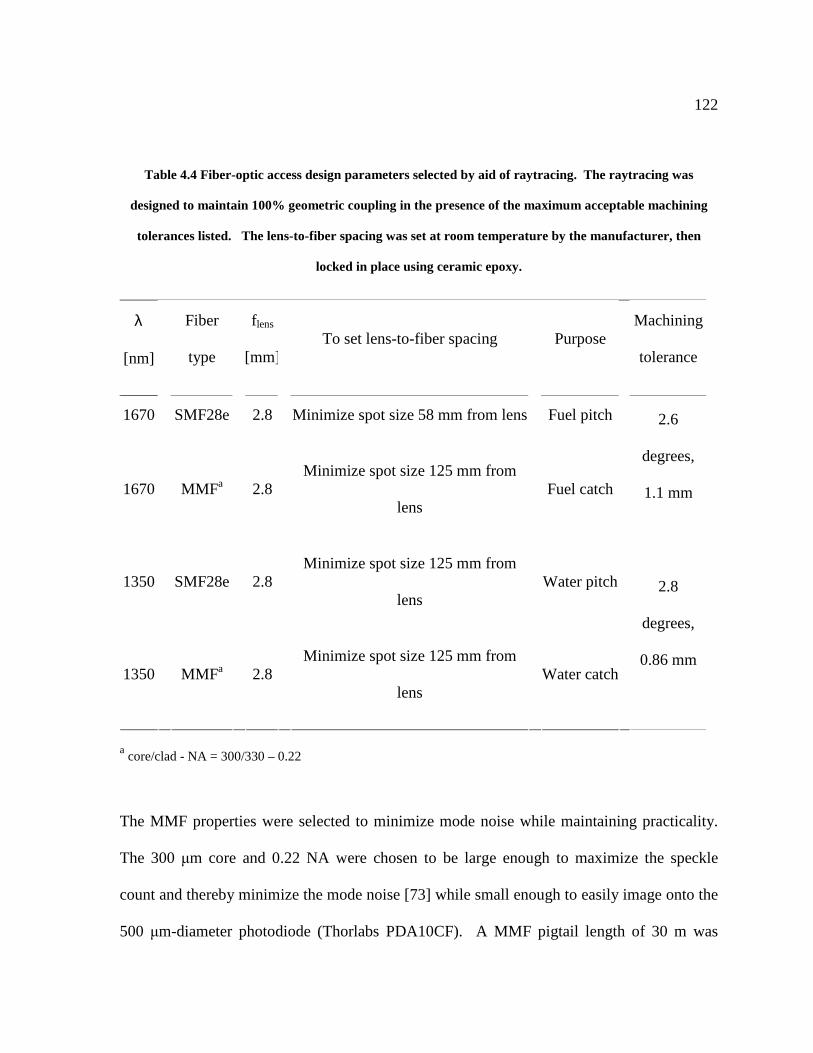
Table 4.4 Fiber-optic access design parameters selected by aid of raytracing. The
raytracing was designed to maintain 100% geometric coupling in the presence
of the maximum acceptable machining tolerances listed. The lens-to-fiber
spacing was set at room temperature by the manufacturer, then locked in place
using ceramic epoxy. ........................................................................................... 122
Page 17
1
CHAPTER 1. INTRODUCTION
The foundation of this research is based on developing a better understanding of how to
perform direct absorption spectroscopy measurements in practical combustion environments
in order to infer gas properties such as temperature and absorber concentration. The work
presented here focuses solely on water vapor absorption but the main ideas should be
tractable to other gas phase species.
Optical diagnostics are a useful tool for performing measurements in practical combustion
environments owing to their inherent ability to probe the sample gas without disrupting the
flow field. Contrast this to other techniques for measuring temperature, such as
thermocouples and sample probe based methods where insertion errors must always be
considered. Direct absorption spectroscopy is especially attractive given the fact that it
provides a measure of the gas properties irrespective of any type of calibration and is
typically only limited in accuracy to the degree in which the absorbers fundamental
spectroscopy is known.
Absorption spectroscopy, specifically H2O absorption, is not without its challenges. Limited
optical access, interferences in the optical path, beamsteering, and a multitude of other bias
and precision error sources tend together to make the act of measuring the spectrum in the
harsh environment of a modern combustion system difficult at best. This is especially true
when the goal is to capture the dynamic nature of these systems requiring overall
measurement rates on the order of tens of kilohertz.
Page 18
2
1.1 MOTIVATION
Many descriptions of gas sensing using diode lasers are not uncommon [1-4]. Much work has
been put forth expanding the applicability of absorption based sensors to practical flows of
interest and much progress has been made in expanding the usefulness of the results obtained
with these sensors [5, 6].
When considering a measurement in a combustion application, one of the first key choices is
the decision of the species to probe. The ubiquity of water vapor throughout the entire
thermodynamic cycle of nearly all practical heat engines makes it a prime candidate. For
instance, it is usually naturally abundant in the intake air streams and is a major product of
combustion of hydrocarbon and other hydrogen-containing fuels. Water also has the
desirable characteristic of having spectroscopic transitions in the spectral region where
modern semiconductor and fiber optic components have undergone much development
owing to the large telecom market that utilizes this same spectral range.
In the past, typical H2O absorption thermometry sensors have been based on measuring two
points in the spectrum (either at a single wavelength or tuning over an entire feature) and
inferring the temperature from the ratio of these measurements [7]. More recently, high speed
thermometry has been performed utilizing broadly tunable lasers and discrete color time
division multiplexed lasers [4,8-10].
Driven by ever advancing laser source development, a methodology for choosing appropriate
wavelengths for optimizing thermometry is needed now more than ever. The sensor design
no longer is limited by the availability of lasers but rather the source can be engineered to
meet the requirements of the sensor. Complicating the wavelength selection problem even
Page 19
3
further is the latest work on transitioning from a single line-of-sight absorption measurement
to a two dimensional measurement through tomographic reconstructions of data recorded
along many lines of sight [11,12]. Hyperspectral tomography based on H2O absorption
spectroscopy offers the promise of truly quantitative 2D representations of the scalar
temperature and concentration field but current reconstruction techniques are costly in
computation and would benefit from measurements that focused on the key points in the
spectrum that offer the best temperature sensitivity.
1.2 THESIS OVERVIEW
The progression of this thesis is as follows:
Chapters 2-4 will introduce novel ideas and practices for absorption thermometry
experiments in practical combustion applications
Chapter 2 offers the reader a background in H2O absorption spectroscopy and how it relates
to inferring gas properties such as temperature and absorber mole fraction
Chapter 3 will offer ideas for solving the wavelength selection problem. Novel
semiconductor based lasers have recently been developed that permit an almost arbitrary
selection of output wavelength versus time [13,14]. The standard 2 color ratiometric
technique doesn’t directly apply to experiments utilizing these multi-color, dynamic light
sources. The selection of wavelengths can pose multiple challenges to the sensor designer
and some rules/guidelines for optimizing these selections are put forth.
Chapter 4 Gives real world practical examples of applying some of the techniques presented
here utilizing some of the latest diode laser based sensors. Three specific measurement
Page 20
4
campaigns are highlighted with each having its own flavor whilst all three sharing the
common theme of inferring the gas temperature and water concentration through absorption
spectroscopy.
Finally, Chapter 5 will conclude this thesis with a summary of main concepts and important
results presented in this thesis with a few recommendations for future work.
Page 21
5
CHAPTER 2. H2O ABSORPTION THERMOMETRY
The use of absorption spectroscopy for measuring gas properties in combustion applications
has been well researched and documented [15-18]. H2O as the target absorber has been given
much attention owing to its ever abundant presence in both the air used in most practical
combustors and as a major product of hydrocarbon combustion [4,16,19-21]. This constant
presence along with available absorption bands in the telecom range of wavelengths (1300-
1550 nm) allows it to be a key probe species when using optical interrogation methods to
study the performance of practical combustors. However, the spectroscopy of the H2O
molecule is not simple and much empiricism must be used to effectively apply these
techniques to real world sensors.
Absorption spectroscopy is a simple linear technique used to study the quantized energy
levels of an atom or molecule. It provides quantitative information about the population of
molecules inhabiting their various energy levels. Assuming local thermodynamic equilibrium
(LTE), the population distribution of these energy levels is governed by the Boltzmann
distribution which is a function of the gas temperature. Temperature can be inferred by
measuring the relative population in two or more distinct energy levels.
There are two primary classes of wavelength management techniques used for gas
thermometry by absorption spectroscopy. One technique involves using multiple, discrete
wavelengths supplied by either single color multiplexed laser sources or a single source that
outputs different colors multiplexed in time and the other technique relies on a continuous
wavelength scan over a broad range of wavelengths. This continuous scanned technique can
be achieved by using either a monochromatic laser that can tune its color in time or using a
Page 22
6
broadband light source and dispersing the light and capturing the various colors in time with
a single detector or capturing multiple colors at the same time with an array detector. Each of
the two primary wavelength management techniques have pros and cons associated with
them and the selection of one over the other may be application driven. With the advent of
current semiconductor gain media and fiber optic technology an almost arbitrary selection of
wavelengths is possible with a single laser source opening the door to more advanced and
innovative thermometry experiments while at the same time complicating the choices to be
made by the sensor designer.
2.1 H2O SPECTROSCOPY FOR SENSOR APPLICATIONS
Perhaps the single most important tool in the experimental spectroscopist’s toolbox is the
Beer-Lambert relation that relates the fractional transmission of a laser beam passing through
an absorbing medium to an absorption coefficient.
0,
exp ( ; )L
o x
Ik y dy
I ν
ν
= −
∫ (2.1)
For a 2D problem, this is the general form of the relation when considering a single absorber
with non-uniform properties. In this equation, Io is the intensity of a laser beam at some
location x before it passes through the absorbing medium, I is the intensity after passing
through the sample, L is the length of the sample where absorption occurs, and kν is the
spectral absorption coefficient. In this form of the equation, the spectral absorption
coefficient is allowed to vary along the length of the beam in the y dimension and thus must
Page 23
7
be included inside the integral over the length. If the gas properties are assumed uniform
along the entire path of the laser beam, this relation can be simplified to the following form.
( )e k LI
Io ν
ν− =
(2.2)
This form of Beer’s law is the one most commonly presented and forms the basis for
quantitative absorption spectroscopy experiments. However, in order to infer gas properties,
the dependence of the spectral absorption coefficient on temperature, pressure, and absorber
mole fraction must be known or reliably predicted. For thermometry experiments, it would
be ideal to measure the absorbance at the wavelengths of interest over the conditions
hypothesized for the problem in order to create an empirical database of spectra to be used
for comparison to further measurements at unknown conditions. In practice, this is often
difficult to obtain under highly controlled conditions and furthermore concomitant measures
of the gas temperature may be unreliable. For these reasons, gas temperature sensing using
H2O absorption spectroscopy is often done by comparing measurements to simulated spectra.
2.2 SPECTRAL DATABASES
For quantitative absorption measurements in practical combustors, the experimental results
usually are the result of comparing the measurements to simulated spectra. In order to
accurately simulate a spectrum, one usually refers to a spectral line list comprised of the
pertinent parameters necessary to evaluate the absorption coefficient. For the water molecule,
two spectral line lists have received the most attention for combustion sensor design.
Page 24
8
2.2.1 HITRAN
The HITRAN (HIgh-resolution TRANsmission molecular absorption database) database is
currently in version 2004 after its beginnings in the 1960s at the Air Force Cambridge
research labs [22]. In addition to H2O, HITRAN contains infrared spectroscopic parameters
for 39 total molecules with the choice of species tailored to the atmospheric sciences
researcher. A variant of the HITRAN database exists that is more suitable to combustion
applications. The HITEMP database uses the same data contained in HITRAN but employs a
smaller line intensity cutoff used for reducing the number of included transitions and this
reduces the chance of an important line missing when simulating high temperature spectra.
The data of relevance to simulating the absorption spectrum included in these compilations
are the line center frequency in units of cm-1, the intensity (also commonly called the line
strength, S), the lower state energy of the transition (E”), and the parameters for estimating
the spectral widths when using a Voigt lineshape function.
2.2.2 BT2
The need for an all encompassing solution for simulating the H2O spectrum has been of great
interest not only for the combustion diagnostic community but for a wide range of
applications and studies such as astrophysics. Building on this need, the THAMOS group at
University College London led by Jonathon Tennyson developed the entirely synthetic H2O
line list BT2 [23]. Using a variational technique in conjunction with highly accurate potential
energy and dipole moment surfaces, the BT2 database is the most complete and accurate H2O
line list to date (221,097 energy levels, cut-offs of J=50 and E”=30,000 cm-1, and totaling
505,806,202 transitions) [23]. With that being said, experimental validation of the database is
Page 25
9
an ongoing project and one that will continue to be necessary since only ~80,000 out of the
approximately 1 billion transitions are known experimentally.
Unlike HITRAN/HITEMP, BT2 does not contain any information related to modeling the
line shape function. For the combustion researcher, this poses added complexity to the sensor
design since most practical combustors operate at pressures at and above where collisional
broadening mechanisms begin to dominate. Assumptions on the lineshape can have greatly
varying results on the calculated absorbance which in turn can substantially affect parameters
inferred from the spectrum such as the absorbers number density and temperature (see
section 4.1). However, the greatly improved line intensities (especially at elevated
temperatures) and higher number of included transitions versus HITEMP has made the BT2
database an invaluable tool to the H2O laser absorption sensor designer.
2.2.3 Comparing the databases
The HITRAN and HITEMP spectral line lists have become an accepted standard for
simulating absorption spectra in combustion studies, especially for the most abundant isotope
of water, 1H216O, even though the primary focus of the HITRAN database is for terrestrial
atmospheric transmission simulations [22]. Discrepancies between measured H2O vapor
spectra and HITRAN simulations are evident when comparing results at typical combustion
temperatures (T >1000 K). The sources of these discrepancies include a lack of quality high
temperature experimental spectra for updating line parameters in HITRAN, and the standard
temperature (To, HITRAN = 296 K) intensity cut-off used when compiling the HITRAN
database. While the HITEMP database doesn’t utilize the same low temperature cut-off, the
database has not been updated as regularly as HITRAN. However, when considering high
Page 26
10
temperature water vapor, HITEMP is the appropriate choice versus HITRAN due to the
inclusion of more lines with high lower state energies [24].
With improvements in light sources and experimental techniques used to acquire absorption
spectra of hot water vapor, there is a strong need for a more complete water line list to more
accurately infer temperature in combustion environments. The BT2 spectral line list of
Barber and Tennyson is a computed line list that is aimed towards providing spectral line
parameters valid for temperatures of up to at least 4000 K and has proven to be more
complete than any other line list in existence [23].
Optical combustion studies using absorption or emission spectroscopy often rely heavily on
spectral line lists of the species of interest. For simulating a detailed absorption or emission
spectrum, the minimum information needed is the line center frequency, < [cm-1], the
temperature dependent line intensity, S(T) [cm/molecule], and the lower state energy [cm-1]
of each transition in a desired spectral range. From this information, a spectrum can be
simulated by dressing each transition with an appropriate line shape function. The HITRAN
database provides information for the pressure and temperature dependent line broadening
coefficients for collision broadened lines to include in the line shape function where as BT2
only provides information for modeling the line position and intensity. To simulate spectra
using BT2, the Doppler line width was computed for each line position and a Voigt profile
was applied using a uniform Lorentzian width based on the average experimental width for
the entire spectrum.
While H2O absorption simulations utilizing HITRAN agree well with experiments at low
temperatures, there are often large discrepancies at high temperatures. The differences arise
Page 27
11
from missing transitions at high rotational quantum numbers, J, and lines from upper
vibrational states. These hot lines and bands provide negligible absorption at atmospheric
conditions but are important in high temperature combustion studies. In order to accurately
simulate high temperature water spectra, the BT2 database employs a J cutoff of 50 and
energy level cutoff of 30000 cm-1, which allows for nearly all lines, especially in the infrared,
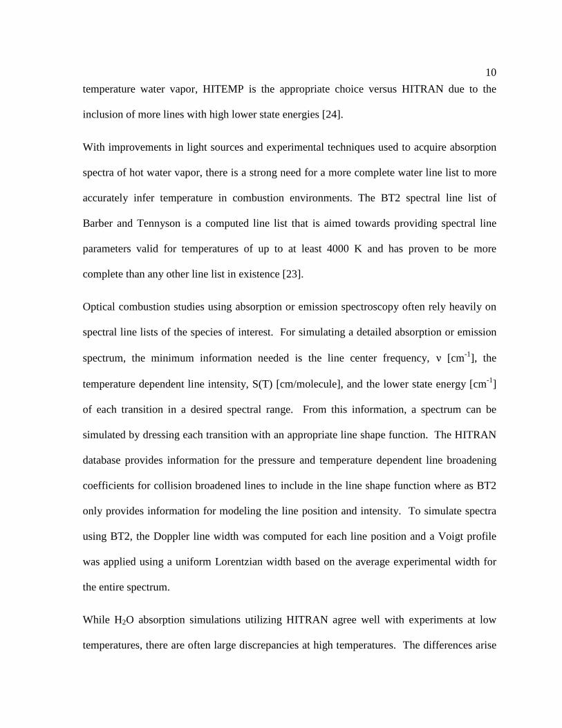
to be listed [23].
Figure 2.1 Shown are the normalized line intensities versus rotational quantum number J for the R
branch of the νννν1+νννν3 band of water (~1330-1370 nm) for the HITRAN (left) and BT2 (right) databases.
The exclusion of high rotational energy lines is evident in the HITRAN data versus the completeness of
the BT2 database.
An example of the completeness of the BT2 database can be seen in the experimental H2O
vapor absorption spectrum recorded during the combustion stroke of a homogeneous charge
compression ignition (HCCI) internal combustion engine. This engine provides nearly
homogeneous gas samples appropriate for single line-of-sight absorption measurements.
Spectra were acquired every 0.25 crank angle degree (CAD) using an advanced swept-
wavelength laser source that scanned from 7245 – 7520 cm-1 every 5 µs [4]. Each spectrum
Page 28
12
was compared to a library of HITEMP simulations to find the best-fit temperature of the
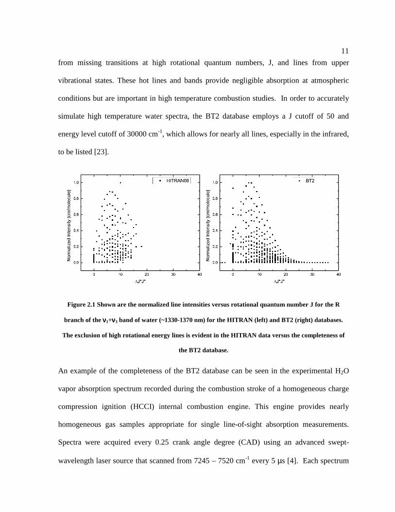
gases in the cylinder. Plotted in Figure 2.2 is a subset of the spectrum measured at top dead
center (TDC) along with simulation results from three different spectral databases; the best
fit HITEMP spectrum at the inferred temperature of 1500 K, a HITRAN simulation at 1500
K and simulations using the BT2 database at temperatures of 1500 K and 2200 K. It is easily
seen that the BT2 simulation provides a better fit at 1500 K than the HITRAN or HITEMP
simulations and even better visual agreement at a temperature of 2200 K. These results
provide evidence of HITRAN’s propensity to bias results toward colder temperatures when
fitting spectra recorded in combustion environments.
0.00
0.04
0.08
0.12
0.16
Measured
HITEMP
HITRAN06
7450 7475 7500 75250.00
0.04
0.08
0.12
0.16
Abs
orba
nce
Optical Frequency [cm-1]
BT2 at 1500 K7450 7475 7500 7525
BT2 at 2200 K
Figure 2.2 Subset of spectrum recorded in HCCI piston engine at top dead center (TDC). The cylinder
pressure was 31.8 bar and the absorption path length 9.5 cm. Plotted against the experimental spectrum
are simulations using multiple databases: HITEMP, HITRAN, and BT2. The HITEMP and HITRAN
simulations are at 1500 K which was the inferred temperature from fitting to the HITEMP library. The
BT2 simulations show improved agreement at 1500 K and even better agreement at 2200 K.
Page 29
13
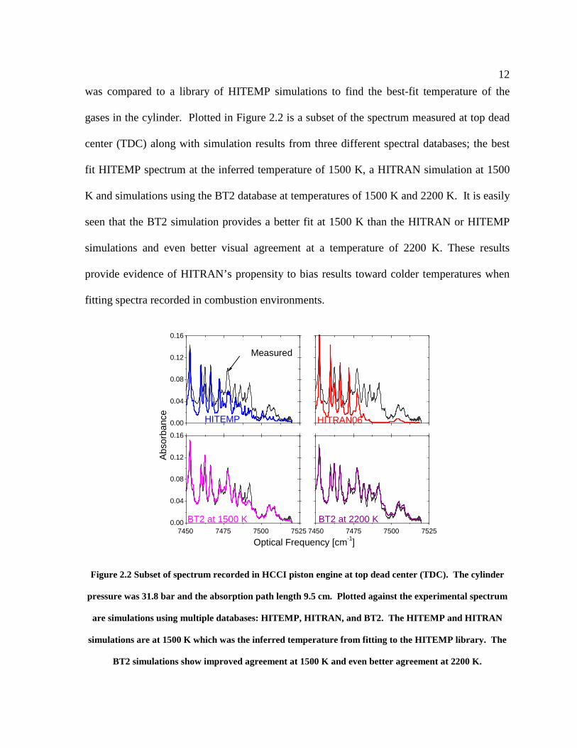
The above result is corroborated by comparisons of best-fit temperatures derived from the
HITEMP and BT2 databases independently. In a steady gas turbine combustor test facility,
H2O vapor absorption measurements were performed using the same swept-wavelength
sensor used to obtain the piston engine data shown in Figure 2.2[25]. During this test, gas
was sampled from the combustion zone and a concomitant temperature was determined from
the gas composition using a chemical equilibrium analysis. Measured spectra were fit to a
library of HITEMP and BT2 simulations in order to infer the temperature. Figure 2.3 shows
the measured temperature from the absorption spectra plotted versus the temperature from
the gas sampling calculations. The equivalence ratio and pressure were varied to produce the
varied operating temperatures. The cold bias of HITEMP results at high temperatures is
again evident, whereas the BT2 results follow the actual gas temperatures to within the
uncertainty visible from the scatter in the data.
1200 1250 1300 1350 1400 1450 1500 15501200
1250
1300
1350
1400
1450
1500
1550
BT2 HITEMP
Tm
easu
red [K
]
Treference
[K]
Figure 2.3 Temperatures inferred from infrared water vapor absorption versus temperatures calculated
from gas sampling. The cold bias is readily seen in the HITEMP results whereas the BT2 data more
closely follows the ideal trend line.
Page 30
14
From experimental evidence, the BT2 database can provide higher temperature results when
compared to HITRAN. This database provides an alternative to HITRAN for either designing
or interpreting results from water vapor absorption experiments conducted at elevated
temperatures. While BT2 does not provide any input parameters for lineshape modeling, the
inclusion of high lower state energy lines improves sensitivity at elevated temperatures. An
assumption of uniform Lorentzian linewidth across spectra spanning ~ 250 cm-1 in the 7200
cm-1 range, although strictly incorrect, resulted in negligible error for the experiments
considered here.
In addition to improved thermometry, there are other benefits of advanced databases such as
BT2. As an example, H2O2 and H2O properties were inferred from experimental spectra
containing contributions from both species. Since H2O was the stronger absorber, the strategy
was to subtract simulated H2O spectra from the measured spectra to reveal H2O2 spectra.
However, intensity imperfections in the HITEMP database caused the residual spectrum to
retain H2O contamination. Using BT2, there is better access to absorbers weaker than H2O
when analyzed in this fashion [26].
2.3 TWO COLOR RATIOMETRIC THERMOMETRY
For a typical H2O absorption experiment, the absorption is quantified using the Beer-Lambert
relation discussed earlier and repeated here in equation 2.3 for simplicity.
( )e k LI
Io ν
ν− =
(2.3)
Page 31
15
This relation relates the ratio of the laser intensity (W/cm2, W/cm2s-1 or W) incident on the
sample (Io) and the intensity after passing through the sample (I) to the product of the length,
L, of the sample and the spectral absorbance coefficient, kν. This product, kνL, is termed the
absorbance, α, and can be related to more fundamental parameters of the species of interest.
( )( ) , , ,i ii
k L N L S T T P xν να φ ν ν = = ⋅ ⋅ − ∑ (2.4)
This equation shows that the magnitude of the absorbance at a frequency, ν, depends on the
absorber number density N, the length of the path in which the absorber is present, and the
weighted sum of line strengths, Si, of absorption transitions in the vicinity of ν with the
weighting factor being determined through a line shape function φ .
In order to make a temperature measurement, two separate wavelengths are chosen and the
ratio of their absorbances is computed. For simplicity, if it is assumed that the chosen
wavelengths are the result of absorbance from a single transition (i.e. the transitions are
isolated) the ratio can be written as:
1 1 1,01 1
2 2 2 2 2,0
( )( )( )
( ) ( )
S TR T
S Tν
ν
φ ν ναα φ ν ν
−= = ⋅
− (2.5)
If it is further assumed that collisional broadening dominates the line shape function and that
the resulting Lorentzian lineshape is the same for both chosen wavelengths, the ratio then
becomes the following pure function of temperature.
1
2
( )( )
( )
S TR T
S T= (2.6)
Page 32
16
The line strength Si(T) can be calculated from the line strength at a known temperature using
the following scaling relationship [27].
1"
0, 0,00
0 0
( ) 1 1( ) ( ) exp 1 exp 1 exp
( )i ii
i i
hc hcQ T hcES T S T
Q T k T T kT kT
ν ν−
− − = − − − −
(2.7)
Inserting equation 2.7 into equation 2.6 yields the following function for the ratio when
neglecting the induced emission (1-ex) terms which is valid given the frequencies and
temperatures involved for near infrared combustion studies (i.e. low upper state populations).
( )" "1 01 2
2 0 0
( ) 1 1( ) exp
( )
S T hcR T E E
S T k T T
= − − −
(2.8)
From this expression, the temperature sensitivity for the chosen line pair can be found by
differentiating equation 2.8 with respect to T.
( )" "
1 2
2
E E RdR hc
dT k T
− =
(2.9)
In practical combustion applications, the assumption of isolated lines is often difficult to use
especially when the pressures are high and significant blending and overlap occurs. In
practice, it’s often easier to work directly with the absorbance values. Typically, the
absorption coefficient is simulated for the wavelengths of interest over a postulated
temperature range and a calibration curve R(T) is computed from which the temperature can
be found.
Page 33
17
2.4 HYPERSPECTRAL THERMOMETRY
Extending the analysis of temperature inference from spectral measurements at two
wavelengths to N wavelengths is not trivial. For instance, assuming the absorber
concentration and the gas pressure is known, measurements of 3 wavelengths results in at
most 3 equations with a single unknown temperature. Therefore, a simple yet robust
methodology is needed for dealing with measurements consisting of multiple wavelengths.
2.4.1 Linear system of equations
One possible method would be to solve a linear system of equations based on simulations at
various temperatures such as Ax = b. A possible formulation is as follows:
1 1 1
1
, , 1 1
, ,
n
m m n
T T
T T n m
k k x T
k k x T
ν ν
ν ν
=
⋯
⋮ ⋱ ⋮ ⋮ ⋮
⋯
(2.10)
Upon solving this set of equations for the vector x, one can make a measurement at an
unknown T (within the calibration range T1…Tm) and multiply the measured row vector by x
to obtain the temperature. If the number of wavelengths and temperatures is the same then
the solution is exact for the temperatures considered but interpolation errors will exist when
attempting to use the result at some other intermediate temperature. In the more general
m n× case, there will be exactly m or n exact solutions depending on which is smaller of the
two as shown in Figure 2.4.
Page 34
18
Figure 2.4 Temperature errors (Tactual – Tmeasured) when using the linear system of equations
(Equation 2.10) to solve for an unknown temperature assuming a perfect measurement (zero noise). The
3 wavelength case (left axis) has 3 points where a perfect solution occurs versus the 5 wavelength case
(right axis) which has 5 zero crossing points. Both of these results used a 101 point temperature vector.
If enough temperatures and wavelengths are used, it is possible to make these errors quite
small and perhaps smaller than a particular design criterion of the sensor. However, even
though this method is suitable for pure temperature measurements it lacks the robustness for
making simultaneous temperature, concentration, and pressure measurements.
2.4.2 Spectral fitting
Another possible technique involves fitting the measured spectrum to a simulated spectrum
by minimizing the sum of the squared errors (SSE) between the two. In practice, the easiest
way to accomplish this task is to build a database of simulated spectra spanning a
temperature range that extends past the predicted temperatures encountered in the
experiment. The database method is especially useful for cases involving lots of wavelengths
Page 35
19
(e.g. broad spanning high pressure spectra or low pressure spectra requiring high resolution).
For these cases, the time penalty occurred in computing spectra on-the-fly usually warrants
the database procedure.
If the concentration or mole fraction of the absorber is unknown, simply minimizing the SSE
as a function of temperature may bias the results if the concentration was maintained constant
in building the database and no other normalization of the data is performed. One way to
alleviate this and to simultaneously solve for the concentration and temperature is to perform
a linear fit between the simulated and measured spectra [28]. The figure-of-merit for this
procedure then becomes the mean-squared-error (MSE) between the best fit line and the
simulated data. As the temperature is varied, the measurement matches a simulated spectrum
when the MSE is minimized. Concurrently, the concentration is inferred by scaling the
known value used in the simulations by the slope of the best fit line.
For simplicity, assume the pressure (spectral line widths) is known therefore requiring a 2D
database (temperature in the vertical direction and wavelength in the horizontal). The process
of inferring the temperature would then be to loop through the N spectra and compute the
MSE versus temperature and this process is depicted in Figure 2.5. The best fit temperature is
then the minimum of this curve. However, because of the discrete temperatures used in the
database, the temperature resolution in picking the minimum will be limited by the resolution
of the database. Adding more temperatures to the database will improve this resolution at the
expense of computation time. However, using a curve fit near the minimum of the MSE
versus T curve and through either interpolation or a derivative of the polynomial fit to find
the minimum, the resolution can be greatly enhanced.
Page 36
20
500 1000 1500 2000 25001.0
2.0
3.0
4.0
5.0
6.0
7.0
8.0
-0.004 -0.002 0.000 0.002 0.004-0.004
-0.002
0.000
0.002
0.004
Poor Fit
abso
rban
ce (
mea
sure
d)
absorbance (sim 367 K)
MSE = 6.82
Good Fit
-0.002 -0.001 0.000 0.001 0.002-0.006
-0.004
-0.002
0.000
0.002
0.004
0.006
MSE = 1
abso
rban
ce (
mea
sure
d)
absorbance (sim 1207 K)
M1207 K
Temperature [K]
MS
E
1000 1100 1200 1300 1400 15000.95
1.00
1.05
1.10
1.15
MS
E
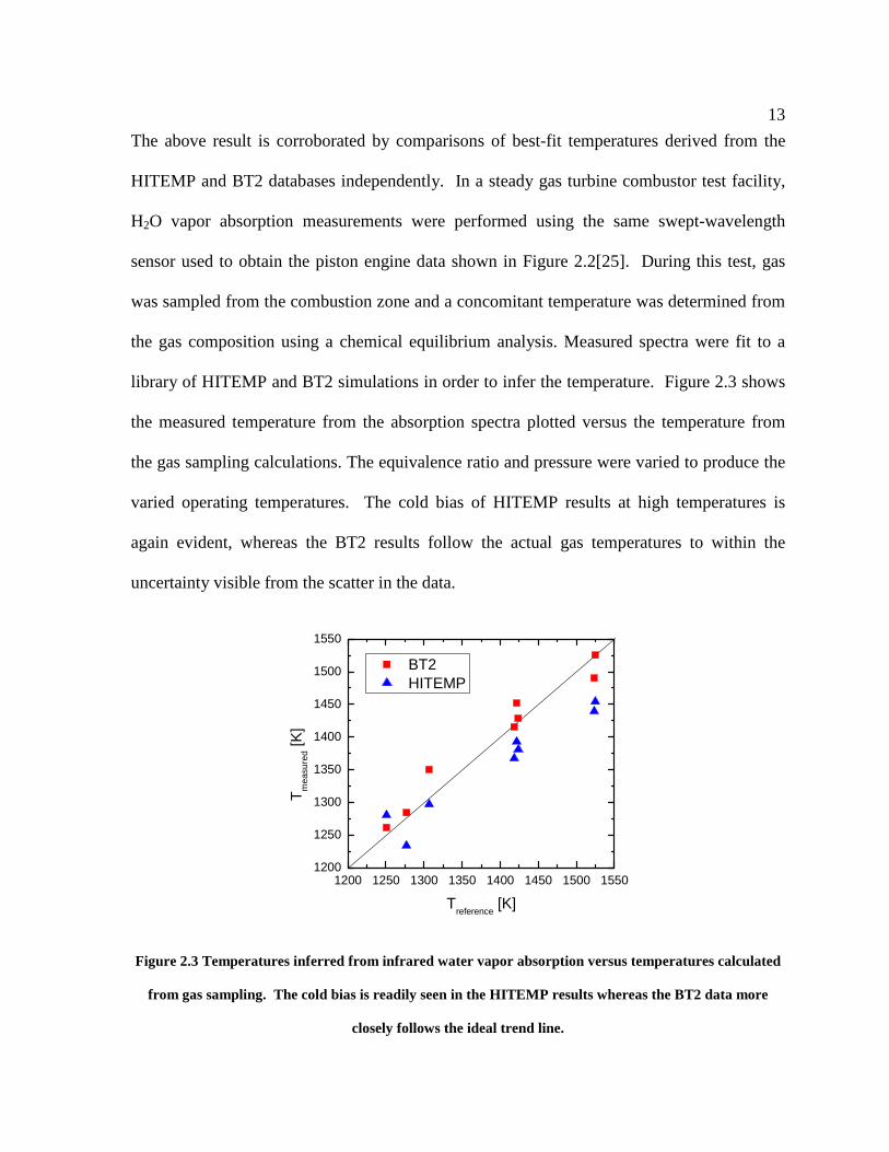
Temperature [K]
Figure 2.5 TOP LEFT: Plotting the measured spectrum at an unknown temperature versus a simulated
spectrum at 367 K showing an example of a poor fit. TOP RIGHT: This fit between the measured and
simulated spectrum at 1207 K is much better as indicated by the MSE of the fit. BOTTOM LEFT: The
arrows point to the MSE values found in the fits in the top two graphs. The fit at 1207 K is shown to be
near the minimum of the MSE versus temperature curve indicating a much better fit. BOTTOM
RIGHT: The final best fit temperature is found by applying a polynomial curve fit near the bottom of the
MSE versus temperature curve.
It is worth mentioning that an optimization routine can be used in place of the brute force
method of converging to the best fit spectrum in the database. For instance, the downhill
simplex routine (non-gradient based unconstrained minimization technique) can be used to
find the minimum MSE and will reduce the number iterations to at least N/2 depending on
the guess value used and the cut-off criteria. However, it may still be worthwhile to compute
the MSE at the neighboring temperatures of the minimum in order to perform the curve fit
for improved temperature resolution. If the database is relatively small (coarse in
Page 37
21
temperature) the use of an optimization routine might not have much added value in relation
to the added complexity of implementation. However, a hybrid routine involving both the
linear system of equations and spectral fitting using the downhill simplex minimization
routine can be formed where the result from the linear system of equations is used as the
initial “guess” value for the downhill simplex routine resulting in faster convergence. This
hybrid method can be especially attractive when processing large experimental data sets.
Page 38
22
CHAPTER 3. WAVELENGTH SELECTION
3.1 INTRODUCTION
Current diode laser technology has allowed novel laser designs of unprecedented speed, low
noise characteristics, and wavelength flexibility to be realized. In the 1300-1500 nm range,
the almost arbitrary choices of wavelengths accessible for H2O absorption sensors for
combustion applications leads to the need for better understanding of the role wavelength
selection plays in the overall performance of the sensor. For instance, one recent laser that
has been developed can provide N discrete (single color) time division multiplexed
wavelengths [13]. These wavelengths can be placed anywhere within the emission band of
current semiconductor optical amplifiers (SOA) thus allowing for unprecedented flexibility
in the design of absorption sensors. Another new laser design can provide 3 distinct,
essentially arbitrary wavelength scans [14]. This laser also has the flexibility in locating the
center locations of the scans to anywhere within the working range of SOAs. This flexibility
from the source side makes the choices of the wavelengths probed for thermometry that
much more important versus previous ideas of scanning an entire rotational branch for
inferring gas properties.
Previously, much work and attention was given to sensors based on 2 wavelengths using a
ratiometric strategy for measuring temperature and from this offered guidelines to aid the
sensor designer in choosing appropriate wavelengths for their application. Nagali et.al.
mentioned that for maximum temperature sensitivity, the derivative of the ratio of two
absorbances with respect to temperature, dR/dT, should be maximized over the range of
temperatures under consideration [29]. Specifically, wavelength pairs were chosen to
Page 39
23
maximize the ratio of relative changes in R and T or (dR/R)/(dT/T). As an add-on
requirement, they also mention that R should lie in the interval (0.25, 4) to assure similar
absorption at both wavelengths but this range was specified arbitrarily.
More recently, Zhou published expanded recipes for guiding decisions on wavelength
selection for situations where one or two (narrowly) tunable diode lasers are used [19,30].
Both recipes were based on a ratiometric approach to thermometry with one approach
applicable to the case of a single laser and the other considering the case of using two
narrowly tunable lasers. The combinations of these findings are outlined below.
1. Sufficient absorption required for high signal-to-noise ratio measurements (SNR > 10
desired although this number is somewhat arbitrary)
2. Transitions are selected to minimize interference from ambient H2O
a. This is mainly for combustion applications where the temperature is much
greater than the ambient
3. The wavelengths of both absorption lines must lie within a single laser scan and not
overlap significantly (not applicable to the 2 laser case)
4. The line pair must represent sufficiently different lower state energies, E”, to yield a
peak height ratio that is sensitive to temperature over the range of consideration
5. The two lines must be isolated from nearby transitions
a. Unless the lower state energies of the overlapping transitions are similar in
lower state energy thus adding constructively and increasing the SNR without
loss of temperature sensitivity
Page 40
24
6. The wavelength must be in the 1.25-1.65 µm range (specific to the lasers considered
in this work)
In conjunction with these guidelines, criterion can be set specific to the absorber considered,
technique employed, and limits of the equipment used. For instance, in step 1, usually the
required absorption can be set by estimating the noise of the experiment and requiring the
absorbance to be at least 10 times this leading to a minimum SNR of 10. It can also be
advantageous to set a maximum absorbance in order to prevent the near-complete extinction
of the probe beam depending on the path length of the beam through the sample gas.
These guidelines form a logical framework for 2 color thermometry but most likely are too
restrictive for the case of N wavelengths. Also, they are based on the idea that the
temperature will be inferred by fitting the measurements to fundamental spectroscopic
parameters and this leads to difficulties such as defining the line strength or lower state
energy for the case of blended spectra. For the case of measurements spanning broad
wavelength ranges at high pressure where significant overlap and blending of features is
prominent, more direction is needed in guiding decisions on wavelength selection for H2O
thermometry.
3.2 SETUP
Of primary concern to the sensor designer is the accuracy and precision of the diagnostic.
H2O absorption based sensors for combustion applications usually are limited to the accuracy
of the underlying spectral parameters used to simulate the spectrum. Steps can be taken to
verify and validate these parameters such as measuring spectra under carefully controlled or
highly known conditions and these experiments have and will continue to be performed
Page 41
25
[18,19,31-34]. Often, though, the difficulty lies in building a test article capable of achieving
the extremes in temperature and pressure encountered in practical combustors such as IC
engines. In addition, even if these thermodynamic states are reached, there may not be a
concomitant technique available for comparison to the optical absorption technique. For
example, thermocouples are often limited by the maximum material temperatures and even
high temperature variants of thermocouples may have large uncertainties at high
temperatures due to uncertainty in the heat transfer correction.
On the other hand, the temperature precision can be optimized through smart design. As
discussed previously, wavelength selection plays an important role in maximizing the
sensitivity of the H2O absorption sensor to temperature and it is not entirely obvious how to
effectively choose wavelengths to guarantee optimal performance for all temperatures
encountered.
To start, a highly simplified model of an ideal diatomic molecule (IDM) was constructed in
order to provide a mathematically simple spectrum. By studying this model certain trends can
be identified and possibly offer guidelines when considering real molecules such as H2O.
3.3 IDEAL DIATOMIC MOLECULE (IDM) MODEL
The simplified model of the ideal diatomic can be specified as a Boltzmann distribution.
( 1)
(2 1)
( )
J
B B
E BJ J
k T k TJ J
J
B
N g e J eF
BN Q Tk T
+− −+ ⋅= = = (3.1)
Page 42
26
This function specifies the fraction of the number of molecules in the Jth state (NJ) to the total
number of molecules (N) where gJ is the degeneracy, EJ the energy of the Jth state, kB is
Boltzmann’s constant, and Q(T) is the partition function at temperature T. In order to
compare the results of studying this model to the actual H2O spectrum, correspondence
between wavelength and absorbance is needed. To do this, the rotational constant, B, is
chosen to be very small such that the ratio B/kB (often termed the characteristic rotational
temperature Θ) is 0.01. This essentially makes the distribution continuous in J and is
analogous to the H2O absorption spectrum at elevated pressure where much blending of
spectral lines occurs and ensures that many different Js (wavelengths) have significant
population over the temperature ranges encountered in most practical combustion
applications. For comparison of this model function with the H2O spectrum, J will be
considered to represent the optical frequency (wavelength) and the fractional population will
be considered to represent absorption. This model contains a further simplification from the
real diatomic spectrum in that all the transition probabilities are considered to be equal.
An example of this function plotted for two different temperatures can be seen in Figure 3.1.
The effect of temperature is easily visible in this figure with more J states becoming
populated with increasing temperature (i.e. increasing population in higher energy states).
This is similar to the effect of increasing temperature in the H2O spectrum with more
wavelengths away from band center (in rovibrational spectroscopy) gaining absorption
strength with temperature.
The aim of studying this simple diatomic model is to gain some insight into how to most
effectively choose wavelengths when performing H2O absorption thermometry. Of particular
Page 43
27
concern is developing a strategy for choosing wavelengths to optimize the temperature
precision when experimental noise is considered.
0 200 400 600 800 10000.000
0.001
0.002
0.003
0.004
1500 K
F =
NJ
/ N
J
500 K
Figure 3.1 Two simulated “absorption” curves of the ideal diatomic model at temperatures of 500 and
1500 K. The absorption spectrum is simulated by using the fractional population in each energy level or
“J state” and assuming the total number density, N, is constant at all temperatures. The effect of
temperature is readily seen as an overall decrease in the peak absorbance value but a larger range of
wavelengths having appreciable absorption.
3.3.1 Case 1: 2 wavelengths, known temperature
For the problem of choosing wavelengths, it is important to maximize the sensitivity dR/dT
of the chosen line pair but a discussion of the influence of experimental noise on the
measurement must also be included in the analysis.
For the ratio measurement of two absorbances, the ratio R can be defined as:
Page 44
28
1
2
1R Rαα
≡ ≥ (3.2)
The uncertainty in R can be found by:
2 2
21 2
1 2
R RR α α
α α ∂ ∂∆ = ∆ + ∆ ∂ ∂
(3.3)
This after some manipulation yields the relative uncertainty as:
2 2
1 2
1 2
R
R
α αα α
∆ ∆ ∆= + (3.4)
If the calibration function R(T) is known, then the uncertainty in temperature can be defined
as:
2 2
1 2
1 2ratio
T RT R
RRT
α αα α
∂ ∆ ∆∆ = ∆ = +∂∂∂
(3.5)
After some manipulation, this relation can be recast into the following form.
2
2 1
2
2
2
ratio
R
TR
T
αα
αα
∆+ ∆ ∆ = ∂ ∂ ∆
(3.6)
This relation shows the precision in temperature not only depends on the sensitivity of the
chosen line pair (dR/dT) but also the ratio of the absorbances and the SNR of the weaker of
the two lines.
For the IDM, the ratio is the following function.
Page 45
29
11 2
2
2 1( 1)1 22 1( , , )
2 1
J JJ J
TJR J J T
Je
−Θ + + ⋅+= ⋅+
(3.7)
Similarly, the derivative of the ratio R with respect to T can be found.
1 2 1 2 11 2 2
2
( 1)( )1 2 2 1( , , ) 2 1( 1)
2 1
J J J J
TR J J T J J J
J JT J T e
Θ⋅ + + −∂ + −= − ⋅Θ⋅ + + ⋅ ⋅∂ +
(3.8)
The aim is to find the best pair of Js that will minimize the function in equation 3.6. For this
relatively simple case of 2 wavelengths at a known temperature, the analytic solution would
prove to be quite cumbersome. Even in doing so, moving to the more interesting but difficult
case of 2 wavelengths over an unknown temperature range this analytic solution would not
provide any more insight. The other alternative is to find the best pair of wavelengths
numerically through an optimization routine. This has the benefit of being relevant for all
possible cases posed for the IDM and will also prove to be highly effective for the more
practical problem of optimizing H2O wavelength selection.
The function in equation 3.6 can be minimized rather easily using any of the standard non-
linear optimization routines presented in most modern scientific computing packages (e.g.
conjugate-gradient, quasi-Newton, Levenberg-Marquardt). However, in order to solve the
more difficult problem of choosing wavelengths when considering a range of temperatures, a
more robust algorithm is needed in order to overcome the possibilities of many local minima.
Genetic algorithms offer the benefit of searching over large domains and are particularly well
suited to optimizing stochastic functions.
For this work the differential evolution (DE) algorithm was used to minimize all objective
functions proposed for finding optimum wavelengths for thermometry. DE finds the global
Page 46
30
minimum of a multidimensional, multimodal (i.e. exhibiting more than one minimum)
function with good probability. The crucial idea is a scheme for generating trial parameter
vectors. DE adds the weighted difference between two population vectors to a third vector.
This way no separate probability distribution has to be used making the algorithm completely
self organizing. For more information about DE the interested reader is refered to the
following sources [35-38].
To find the best 2 wavelengths for optimizing the precision of temperature measurements for
the simple case of a single known temperature, the function in equation 3.6 is used as the
objective function with the added constraint that J must lie in the domain (0,1000). To
implement this inequality constraint, the objective function is modified by adding an
additional case statement that checks the parameters chosen by the DE algorithm and applies
a penalty if the constraint is not satisfied. Also, the noise terms are assumed to be fixed and
the same for all wavelengths. This assumption is based on the fact that the minimum
detectable absorbance (MDA) will be approximately constant across the spectrum.
The best wavelength pairs at 5 different temperatures are shown in Figure 3.2. The visible
trend is the best wavelength pairs (represented as the vertical drop lines) moving to higher
energy levels with increasing temperature. From this figure, it is not obvious as to why the
particular wavelengths chosen are better than other choices but comparing the wavelengths
from the DE to those obtained with a conjugate-gradient method give the same results. The
conjugate-gradient method works well for this simple case since the objective function is
smooth and exhibits a single global minimum.
Page 47
31
0 200 400 600 8000.000
0.001
0.002
0.003
0.004
1500 K1250 K
1000 K
750 K
F =
NJ
/ N
J
500 K
Figure 3.2 Showing the best two Js (wavelengths) that will maximize the precision of the temperature
measurement for the prescribed temperature. The visible trend is the wavelengths of the best pair
moving to higher energy levels with increasing temperature.
Once the best wavelength pairs at a specific temperature have been found, it is possible to
calculate the performance over a range of temperatures. Figure 3.3 shows the performance
curves for the wavelengths chosen at a single, specified temperature over a range of
temperatures. It is easily seen that the performance is optimized at the temperature for which
the wavelengths were chosen. It is also interesting to note that the performance is always a
little better for a specific line pair at temperatures slightly lower than those used for the
optimization. This is attributed to the SNR improving for the slightly cooler temperatures
without sacrificing sensitivity (i.e. d(dR/dT)/dT < d(SNR)/dT) over a small dT).
Page 48
32
400 600 800 1000 1200 1400 1600 1800 20000.01
0.1
1
1250 K1500 K
1000 K750 K
∆T/T
[%]
temperature [K]
500 K
Figure 3.3 Temperature precision performance of the best line pairs chosen for a specific temperature
using a fixed noise level of 1E-6. The curves show that the performance is optimized at the temperature
considered for a particular line pair. What is also evident is the performance of a particular line pair is
always a little better at slightly colder temperatures than the temperature used for optimizing.
It is possible to reformulate the objective function into a form that allows a better way of
graphically depicting the choice for the best 2 wavelengths at a particular temperature. To do
this, the derivative, dR/dT, can be rewritten in terms of absorbance.
' '
'1 1 2' 22 2
dR d
dT dT
α α α ααα α
= − ≡ (3.9)
Upon substituting this into equation 3.6 and assuming the noise terms are equal leads to the
following relation.
Page 49
33
2
' '1 2
1ratio
RT
R
αα α
∆ +∆ =−
(3.10)
This equation shows that minimization of ∆T requires the chosen wavelengths to have the
largest difference between their derivatives with respect to temperature in order to maximize
the denominator. From this, the ratio of the absorbances should also be maximized to the
degree that further increase in R doesn’t penalize by making the numerator too large.
To visualize this, the spectra along with the derivative spectra are shown in Figure 3.4. From
the derivative spectrum picture, it is easily seen that the best choice for wavelengths at a
particular temperature are those that exhibit the largest change in absorbance with a change
in temperature at the temperature considered (i.e., the peaks and valleys of the derivative
spectrum). The final choice of the best 2 wavelengths do not converge exactly to the peak
and valley of the derivative spectrum due to the ratio of the absorbance becoming the
controlling term as the ratio differs further from 1.
Page 50
34
0 100 200 300 400 500 600 700-6x10⁻⁶
-4x10⁻⁶
-2x10⁻⁶
0
2x10⁻⁶
4x10-60.000
0.001
0.002
0.003
0.004
dF/d
T [K
-1]
J
1500 K1250 K
1000 K
750 K
500 K
F =
Nj /
N
Figure 3.4 TOP PANEL: Spectra at various temperatures showing the best line pairs chosen for
optimizing the temperature precision. BOTTOM PANEL: Derivative spectra showing the same chosen
line pairs. The choices for the best line pairs at a specific temperature tend to fall near points where the
largest change in absorbance with a change in temperature occurs.
Up to this point, the choice of the best 2 wavelengths for minimizing the uncertainty in
temperature at a specific temperature has been decided by minimizing the function in
equation 3.6 through the use of a non-linear optimization routine. This method works quite
well and converges quickly owing to the relatively simple objective function. In addition, the
Page 51
35
derivative of the spectrum with respect to temperature offers a way to quickly view
wavelengths that will provide optimal sensitivity to temperature. However, neither of these
methods lead to a direct view of how the lower state energy plays a role in wavelength
selection.
Another way of viewing this problem is through the use of the ratio spectrum. For this IDM
model, this leads to the following relation.
1 1(2 1)( )
( )(2 1)
B
ref B ref B
refB ref
ref
E
k T Ek T k T
E
k T
J e TF T T eF T T
J eT
− −
−
Θ+ ⋅ ⋅= = ⋅
Θ+ ⋅ ⋅
(3.11)
Taking the natural logarithm of this expression gives the following useful relation.
( ) 1 1
ln ln( )
ref
ref B ref B
TF TE
F T T k T k T
= + −
(3.12)
From equation 3.12, one can anticipate that a graph of the natural log of the ratio spectrum
versus lower state energy (E) is linear with the slope given by a simple function of
temperature only.
1 1
B ref B
slopek T k T
= − (3.13)
This is confirmed in looking at Figure 3.5 below.
Page 52
36
0 1000 2000 3000 4000 5000 6000 7000 8000
0
5
10
15
20
25
500 K
1000 Kln
[ F
(T)
/ F(T
ref)
]
E [cm-1]
1500 K
(1/kBT
ref - 1/k
BT)
Figure 3.5 Linear relationship between the lower state energy E and the natural log of the ratio of spectra
computed at T and a reference T. The slope is determined by a simple function of temperature only.
Another way then to define the uncertainty in temperature is by describing the uncertainty in
measuring the slope of this linear function.
The slope for a measurement at 2 wavelengths can be defined as:
2 2 1 1
2 1
ln( ( )) ln( ( )) ( ( )) ( ( ))ref refF T F T F T F TS
E E
− − +=
− (3.14)
The uncertainty in measuring the slope will only depend on the uncertainty in the
measurement of F1 and F2.
2 2
21 2
1 2
S SS F F
F F
∂ ∂∆ = ∆ + ∆ ∂ ∂ (3.15)
Page 53
37
This leads to following relation for the uncertainty in S where F has been replaced byα for
convenience in comparing to previous relations.
2 2
1 22 1
1 2
1( )S where E E E
E
α αα α
∆ ∆∆ = + ∆ = − ∆ (3.16)
From this the uncertainty in temperature can be defined as:
2 22
1 2
1 2
BB
T k TT S
S E
α αα α
∂ ∆ ∆∆ = ∆ = + ∂ ∆ (3.17)
The subscript B on the temperature uncertainty is there owing to the fact that this equation
represents a Boltzmann limit in the uncertainty in temperature when considering
experimental noise. This relation directly shows that the choice of 2 wavelengths for
optimizing the uncertainty in temperature should be made by maximizing the difference in
lower state energies while keeping the SNR of the two measurements at acceptable levels.
Upon comparing the relation in 3.17 to the relation in 3.5 it is shown that temperature
sensitivity for the ratiometric formulation is optimized for a particular line pair when
2
BR k TR ET
=∂ ∆∂
(3.18)
This is exactly the same relation derived in equation 2.9 and it shows that the temperature
sensitivity of a specific line pair provides a good starting point for choosing wavelengths
when optimizing 2 color thermometry at a single temperature.
Page 54
38
3.3.2 Case 2: 2 wavelengths, unknown temperature
The previous case of choosing 2 wavelengths at single, known temperature provided a good
starting point for developing strategies for choosing wavelengths for more interesting and
practical cases. For instance, the next logical progression would be deciding the best 2
wavelengths for optimizing thermometry at an unknown temperature within some expected
range of temperatures to be encountered in an experiment.
In order to do this, the objective function for the single temperature case will have to be
slightly modified to include the range of possible temperatures. Instead of directly
minimizing the relation in equation 3.5, a possible new objective function to be minimized is
the sum of the relative uncertainties over a specified range of temperatures.
2 2
1 2
1 2
ratio
T T
T RRT TT
α αα α
∆ ∆ ∆= +∂∂
∑ ∑ (3.19)
An example of the performance results obtained after minimization of this objective function
is shown below in Figure 3.6. Also shown in this figure are the results from the single
temperature case. It is interesting to note that the relative uncertainty for the line pair chosen
over the temperature range (500-1500 K) performs similarly to the results for the single
temperature case at the geometric mean of the temperature range considered.
Page 55
39
400 600 800 1000 1200 1400 1600 1800 20000.01
0.1
1
optimized 500 - 1500 K
1250 K1500 K
1000 K
750 K
∆T/T
[%]
temperature [K]
500 K
Figure 3.6 Relative uncertainty in temperature versus temperature for the 2 wavelength case. The result
for the best line pair when considering the range of temperatures (500-1500 K) is shown along with the
results obtained when considering a single temperature.
However, the actual wavelengths chosen for the temperature range case do not correspond to
any choices found for a single temperature case. Put differently, the best two wavelengths
found when optimizing the temperature precision over a range of temperatures cannot be
found by optimizing the precision at one specific temperature. When considering a range of
temperatures, it is best to choose the wavelengths based on the performance over this range.
However, this effect becomes less pronounced as the temperature range considered is
reduced. On the other hand, the difference in the wavelengths chosen for the wide range
(500-1500 K) are not too different from the wavelengths chosen at 1000 K. This could
Page 56
40
provide a method for quickly identifying possible candidates without having to consider the
entire range.
0 200 400 600 8000.000
0.001
0.002
0.003
0.004
optimized
(500-1500 K)
1500 K1250 K
1000 K
750 K
F =
NJ/N
J
500 K
Figure 3.7 The line pair chosen to optimize the relative uncertainty over a range of temperatures is
plotted along with the line pairs chosen for the single temperature cases. The choice of the best line pair
does not correspond to the best pair at any single temperature.
The two cases considered up to this point have only provided a method for choosing two
separate wavelengths for making temperature measurements. In practice, this amounts to
using two fixed wavelength lasers aligned to the features of interest or using one laser
capable of outputting two separate wavelengths multiplexed in time. However, using tunable
lasers capable of covering a range of wavelengths it is possible to measure the spectrum at
more than two discrete points. This is also true for a single laser capable of outputting N
discrete wavelengths. It is therefore desirable to have a method of choosing wavelengths
Page 57
41
when considering the N wavelength case and even more so, having a means to directly
quantify the results in order to compare the 2 wavelength case to the N wavelength case.
3.3.3 Case 3: N wavelengths, known temperature
In order to solve the N wavelength selection problem, a new objective function needs to be
specified that is capable of including the measurements at N wavelengths. The two color
ratiometric technique of the previous sections does not have an obvious means of extending
the analysis to N wavelengths. From previous work dealing with multiple color absorption
measurements, the temperature is inferred through a spectral fitting routine similar to what
was outline in section 2.4.2. One possible formulation of an objective function for N
wavelengths is to repeatedly compute the temperature of a N wavelength spectrum with
added Gaussian white noise and from which the standard deviation in the computed
temperatures can be obtained. This type of an objective function is very close to what would
be realized in an actual experiment.
In order to estimate the number of iterations needed to estimate the variance of the
temperature results within 10% of the true value with 95% confidence the following relation
is used based on the Student t test [39].
{ }2 2 2ˆ( ) 1.96 2 / 0.95P kσ σ σ− ≤ = (3.20)
The requirement of at most 10% error in the variance estimate gives the following:
( )2 2
2
ˆ0.1
σ σ
σ
−= (3.21)
Page 58
42
Which leads to setting:
1.96 2 / 0.1
800
k
k
=≈
(3.22)
Therefore, the number of iterations needed to accurately estimate the standard deviation in
temperature is approximately 800. The procedure then for finding the best wavelengths for
the N wavelength case at a known temperature using the iterative least square fitting (iLS)
objective function is then:
1. Compute the “measured” absorbance for N wavelengths at temperature T and a
database N wavelengths at M temperatures surrounding T
2. Add a prescribed amount of Gaussian white noise to the computed spectrum
3. Find the best fit temperature of the measured spectrum by least square fitting to the
database of spectra
4. Repeat k times and calculate the standard deviation of the inferred temperatures
Therefore, for each population generation of the DE optimization routine, roughly M*k
calculations are needed for one calculation of the objective function. The results of
optimizing this objective function for the single temperature case of 500 K for 2,3,4, and 10
wavelengths are shown below in Figure 3.8 and Figure 3.9.
Page 59
43
200 400 600 800 1000 1200 1400 1600 18000.002
0.004
0.050
0.100
0.150
full spectrum
1000 unique
wavelengths
∆T ratio function LS fitting
4 wavelengths
(LS fitting)
3 wavelengths
(LS fitting)
10 wavelengths
(LS fitting)
∆T/T
[%]
temperature [K]
2 wavelengthssimple diatomic modelfixed noise level (1E-6)optimized for T = 500
Figure 3.8 Relative uncertainty performance results for the N wavelength case when optimizing at a
single temperature (500 K). The 2 wavelength case is also shown with the results obtained both through
fitting and through the ratio function derived earlier and good agreement is found between the two. At
fixed performance (i.e. same noise level assumed for all number of wavelengths) adding wavelengths
improves the fidelity of the measurement.
For fixed noise level for all wavelength count cases considered, the general trend of adding
wavelengths is to improve the fidelity of the measurement. As a check, it was verified that
the ∆Tratio function used in the 2 wavelength case and spectral fitting gave the same results
when considering the two wavelength case.
In looking at the actual wavelengths chosen in Figure 3.9, the visible trend is the additional
wavelengths should be located near the optimum pair selected in the 2 wavelength case. This
makes sense for the single, known temperature case in that these two points on the spectrum
Page 60
44
offer the best sensitivity to temperature. The only other logical choices would be closer to the
peak for perhaps increased SNR but in looking at the derivative spectrum this would cause
those choices to have less sensitivity with temperature and as was shown earlier, the
differences in the lower state energy would be decreased again leading to less sensitivity in
temperature.
0 100 200 300 400 5000.000
0.001
0.002
0.003
0.004
2 λs 3 λs 4 λs 10 λs
F =
NJ/N
J
temperature = 500 K
∆TLS fitting
-6x10⁻⁶
-4x10⁻⁶
-2x10⁻⁶
0
2x10⁻⁶
4x10⁻⁶
dF/dT dF/dT
[K-1]
F
Figure 3.9 Final wavelength choices when optimizing 2,3,4 and 10 wavelengths at 500 K. For the IDM
model, adding more wavelengths tends to putting more wavelengths near the choices found in the 2
wavelength case. The wavelengths found in the 2 wavelength are the critical wavelengths.
It is unclear if the wavelengths selected through this objective function are actually the best
choices. The choice of optimizing an objective function that was based on estimating the
variance to within 10% leads to an unclear estimate of the global optimum. Also, the method
of estimating the variance through iteration is costly in computation time (M*k computations
Page 61
45
for this N wavelength objective function versus one computation for the 2 wavelength case).
Therefore a better objective function is desired.
Building on the idea presented in deriving the Boltzmann limit for temperature uncertainty
for the two wavelength case given in section 3.3.1, a new expression for the temperature
precision for N wavelengths can be developed. As it was shown, the uncertainty in
temperature can be derived by estimating the uncertainty in measuring the slope of the graph
of ln(α /α ref) versus E” (see Figure 3.5). To extend this analysis from 2 to N wavelengths,
the slope can be calculated using least squares regression. It should be stated that the idea of
using the Boltzmann plot (ln(α / α ref) vs. E”) is not new. References of this idea can be traced
back to at least Herzberg in his book on the spectra of diatomic molecules [40].
The least square solution can be found by minimizing the sum of the square of the residuals
between the measured points and the best fit line.
( ) 22 ln( / )ref i ii
R b sEα α = − + ∑ (3.23)
Taking the partial derivative of this equation with respect to m and s leads to the following
equations that can be used to find the best m and s that will minimize R2.
2
2
2 (ln( / ) ) 0
2 (ln( / ) ) 0
ref i ii
ref i i ii
Rb sE
b
Rb sE E
m
α α
α α
∂ = − − − =∂
∂ = − − − =∂
∑
∑ (3.24)
Upon solving these two equations for m and s leads to the following relation for the slope s.
Page 62
46
2 2
ln( / ) ln( / ) Nref ref
ii
E N Es where x x
E N E
α α α α−= =
−∑ (3.25)
The variance in measuring the slope can be defined as:
2
2i
i i
ss α
α ∂∆ = ∆ ∂
∑ (3.26)
with the partial derivatives given by:
2 2
1 i
i i
E NEs
E N Eα α −∂ = ∂ −
(3.27)
Finally, the unweighted least squares (uwLS) uncertainty in temperature can be given by:
( )22 2
2 2
iBuwLS i
i i
T k TT s E NE
s E N E
αα
∆∂∆ = ∆ = − ∂ −∑ (3.28)
The absolute value in the denominator of this expression is there as a reminder that this term
was factored out of the square root.
In comparing this expression to the 2 color Boltzmann expression given in equation 3.17 a
few key similarities are evident. For one, the kBT2 term is still present and in fact is a factor
that will always be present for a system that follows Boltzmann statistics. Also, when 2
wavelengths are considered, this expression becomes identically equal to the expression in
equation 3.17 therefore making this relation a more general expression to use when selecting
any number of wavelengths.
Page 63
47
The usefulness of this expression becomes more evident when used as the objective function
for selecting the best wavelengths. Instead of the M*k calculations needed for one evaluation
of the least square fitting objective function used above, a single calculation can be
performed to give the value of the objective function for a single set of parameters in the DE
genetic algorithm.
Aydin et.al. used a similar idea in measuring electron temperatures in laser induced plasmas
[41]. In this work, they first systematically identified a collection of isolated spectral
emission lines when considering the FE I and FE II electronic bands. Upon making a set of
measurements, spectral lines with the highest average deviations from the Boltzmann plot
regression function are slowly discarded until a threshold value for the coefficient of
determination is exceeded. This is essentially a wavelength selection procedure Ex Post
Facto. The novelty of the proposed method in this work is using the Boltzmann plot idea for
selecting wavelengths up front when experimental noise is considered in order to optimize
the thermometry results.
The previous example of finding the best wavelengths at a known, single temperature was
repeated with the new ∆TuwLS objective function. These results can be seen below in Figures
Figure 3.10 and Figure 3.11. The performance curves for the two methods are identical for
the 2 wavelength case in that both methods chose the same 2 colors found using the ∆Tratio
function earlier. However, for 3 wavelengths and more, the performance of the ∆TuwLS is
better. This is attributed to the fact that the uwLS function only gave 2 unique colors for each
number of wavelengths considered. This is due to the fact that for a known temperature, there
are 2 unique wavelengths that will optimize the precision of the temperature measurement.
Page 64
48
Repeating the measurement of one or both of the wavelengths is in essence averaging the
measured values and increasing the SNR of the 2 critical wavelengths.
200 400 600 800 1000 1200 1400 1600 18000.001
0.010
0.100
1000 wavelengths(300 λ1, 700 λ2)
100 wavelengths(30 λ1, 70 λ2)
full spectrum1000 uniquewavelengths
∆T ratio and uwLS functions LS fitting
4 wavelengths3 wavelengths
10 wavelengths(3 λ1, 7 λ2)
∆T/T
[%]
temperature [K]
2 wavelengthssimple diatomic modelfixed noise level (1E-6)optimized for T = 500
LS fitting
∆TuwLS function
Figure 3.10 Comparison of the results of the N wavelength, single temperature case using the iLS
objective function and the ∆TuwLS objective function. For 2 wavelengths, these two objective functions
give the same results and are both equal to the results given using the ∆Tratio function. However, as N is
increased from 2, the two methods diverge with the ∆TuwLS function leading to a selection of wavelengths
with better performance.
In looking at the actual wavelengths given by the uwLS function, the trend that is visible is
that as N is increased the optimal wavelengths tend to converge to the peaks on the derivative
spectrum and the splitting ratio tends to a 30-70 split with 30% of the N wavelengths used for
the stronger line near J of 100 and 70% of the N wavelengths located near 330.
Page 65
49
80 100 280 300 320 340 360 3800.000
0.001
0.002
0.003
0.004
7,701
32
11
∆TuwLS function
2 λs 3 λs 4 λs 10,100 λs
2 λs 3 λs 4 λs 10 λs
dF/dT
[K-1]
dF/dT
F
dF/dT
F =
NJ/N
J
temperature = 500 K
brea
k re
gion
F
∆TLS fitting
1
3,30
80 100 300-6x10⁻⁶
-4x10⁻⁶
-2x10⁻⁶
0
2x10⁻⁶
4x10⁻⁶
Figure 3.11 This figure shows the best wavelengths chosen using the ∆TuwLS function and also shows the
previous results obtained through the least squares fitting function. For each number of wavelengths
considered, the ∆TuwLS function gave just 2 independent wavelengths. For instance, the 3 wavelength case
shown in blue squares is actually 2 unique colors (1 near 100 and 2 near 320).
This case study of N wavelengths at a known temperature has shown that there are 2 unique
colors for optimizing the temperature precision and the choice of the two depends on the
timing characteristics of the laser used. For instance, if 2 separate lasers are used and the
splitting ratio of time spent measuring each one is 50/50; the results found when considering
2 wavelengths should be used. Otherwise, if the lasers can be timed such that 30% of the
allowed measurement time is used for λ1 and 70% for λ2 then the results of the 10 and 100
wavelength case should be used. This, of course, assumes that the noise performance at each
Page 66
50
of the two colors is the same and if not, then the actual noise characteristics should be
included in the optimization routine.
3.3.4 Case 4: N wavelengths, unknown temperature
The previous section only considered the best wavelengths when optimizing for a single
temperature. In practice, the temperature is usually unknown and depending on the device
under test, may vary considerably. The more interesting case would be selecting wavelengths
when considering a range of temperatures.
Before specifying the objective function to be used to find the best wavelengths over a range
of temperatures, the performance of the uwLS function should be tested when using the
entire spectrum (i.e. measuring at all the possible wavelengths in order to cover the entire
range of lower state energies) and compared to the results obtained by directly fitting the
spectrum through either least squares or minimizing the sum of the square errors (SSE).
Page 67
51
400 600 800 1000 1200 14000.002
0.004
0.010.1
110
1001000
10000100000
10000001E71E8
∆TuwLS function
∆TSSE fitting
∆T/T
[%]
temperature [K]
0 200 400 600 800 10000.000
0.001
0.002
0.003
0.004
1500 K
1000 K
F =
NJ /
N
J
500 K
Figure 3.12 Results of the uwLS function and SSE fitting showing the large discrepancies between the
two when calculating the relative uncertainty for the entire spectrum (1000 wavelengths spaced at
increments of 1).
As can be seen in Figure 3.12, the ∆TuwLS function blows up at low temperatures and is still
quite different than the SSE fitting results at high temperatures. This is attributed to the fact
that the uwLS function is unfairly biased by the large number of wavelengths exhibiting
nearly zero absorbance. This is especially true at the colder temperatures where
approximately 50% of the wavelengths are zero plus noise. When inferring the temperature
through least squares fitting by comparing the measured spectrum to a database of spectra at
different temperatures, the fitting is inherently weighted by the magnitude of the absorbance
values. This is due to the fact that the zero absorbance points are all localized to a single
region on the plot of the measured absorbance versus reference absorbance and so the bulk
Page 68
52
effect is an ensemble average over these zero points thus reducing their effect on the fidelity
of the fit. This effect can be seen in Figure 3.13 near the (0,0) point where the zero
absorbance points all lie approximately in a vertical plane at x = 0 due to noise occurring
only in the measured spectrum (y dimension).
0.000 0.002 0.004
0.000
0.002
0.004
mea
sure
d ab
sorb
ance
(T
unkn
own)
simulated absorbance (Tknown
)
measured vs simulated best fit line
Figure 3.13 Example of the least square fitting method to infer temperature. The measured absorbance at
some unknown temperature is plotted against a simulated spectrum at a known temperature and the best
fit line is computed from this scatter plot. Note that the points in the spectrum that have very low
absorbance (near (0,0) point) all fall in a single vertical plane and hence the fit is inherently weighted by
the magnitude of the absorbance.
In order to construct a better estimate of the temperature uncertainty, the least square residual
equation shown in equation 3.23 can be modified to include weighting of the regression. The
new least squares residual equation now looks like this:
Page 69
53
( ) 22 ln( / )i ref i ii
R w b sEα α = − + ∑ (3.29)
A weighting factor, wi, has been added to more accurately reproduce the method of inferring
temperature through spectral fitting.
Carrying out the analysis in the same fashion as before, leads to the following weighted least
squares (wLS) function for the temperature uncertainty.
( )22 2
22
i iBwLS i
i i
wT k TT s wE wE
s wE w wE
αα
∆∂∆ = ∆ = − ∂ −∑ (3.30)
The appropriate choice for the weighting factors should be based on the magnitude of the
absorbance and these weights should be positive. In order to meet these requirements a
possible formulation for the weighing factors is:
2
2i
ii
i
wα
α=∑
(3.31)
Reapplying this wLS function to the full spectrum data and comparing the relative
temperature uncertainty results to those obtained through spectral fitting yields much better
agreement and this can be seen in Figure 3.14.
Page 70
54
400 600 800 1000 1200 14000.002
0.004
0.006
0.008
0.010
∆Tmx+b fitting∆TwLS function
∆TSSE fitting∆T/T
[%]
temperature [K]
0 200 400 600 800 10000.000
0.001
0.002
0.003
0.004
1500 K
1000 K
F =
NJ /
N
J
500 K
Figure 3.14 Comparison of the results of the wLS function versus SSE and mx+b spectral fitting shows
much better agreement as compared to the uwLS function when calculating the relative uncertainty for
the entire spectrum (1000 wavelengths spaced at increments of 1).
The wLS function for the temperature uncertainty follows the same trend as two different
methods of spectral fitting. The observed difference between the SSE method and mx+b
method is attributed to the same effect that caused the uwLS function to misbehave when
considering many wavelengths with very low (~0) absorbance. The SSE method just
considers the errors due to noise between the measurement and the simulation and can be
unfairly biased when many points with low SNR are included. The least square solutions
when spectral fitting (whether fitting to y=mx or y=mx+b) have an inherent built in
weighting mechanism in that points with low absorbance (low SNR) are essentially averaged
in the fit and through iteration to infer temperature have an equal effect at all temperatures.
Page 71
55
From a practical standpoint, the 2 parameter least square solution (mx+b) should be
considered first since it will be less sensitive to baseline errors which are almost always
present when measuring an absorption spectrum. However, if a reduced wavelength count
system is being used, the baseline is reliably measured, and the wavelengths have a SNR
greater than 1, the SSE and both the 1-parameter and 2-parameter least square solution give
equally reliable results. This is also true for the uwLS and wLS functions for predicting the
temperature precision of a measurement and therefore the results for the N wavelength,
known temperature case above using the uwLS function are still the correct results.
There is one caveat for the spectral fitting methods if the absorber mole fraction is unknown.
The SSE method as described would need to be modified by including some form of
normalization to account for bias from the measured and simulated absorbances being of
different magnitudes. For instance, the error between the measured and simulated spectra
would be dominated by a global difference in absorption strength and not posses a minimum
in the SSE versus temperature curve. In practice, either of the least square solutions is
recommended first.
Now that a final and more appropriate function for estimating the precision of a temperature
measurement has been formulated, the case of N wavelengths at some unknown temperature
can be considered. The objective function to be minimized for this case is similar to the 2
wavelength case at an unknown temperature.
( )2
2
22
wLS i iBi
T T i i
T wk TwE wE
T wE w wE
αα
∆ ∆= − −
∑ ∑ ∑ (3.32)
Page 72
56
Similar to before, the objective function is chosen as the sum of the relative uncertainty over
a range of temperatures. Applying this objective function to the DE optimization scheme
yields the results shown in Figure 3.15
400 600 800 1000 1200 1400 1600 1800 2000 2200 24000.001
0.010
0.100
∆Tmx+b fitting
∆TSSE fitting∆TwLS function
full spectrum100 uniquewavelengths
full spectrum1000 uniquewavelengths
4 wavelengths3 wavelengths
10 wavelengths
∆T/T
[%]
temperature [K]
2 wavelengths
simple diatomic modelfixed noise level (1E-6)
optimized for T = 500-1500 (100 K increments)
optimized for T = 300-2000
Figure 3.15 Temperature precision results of the N wavelengths, unknown temperature case for the IDM
model. Again, it is evident that adding more wavelengths results in better performance across the entire
temperature range considered when adding wavelengths has no adverse effect on the measurement (i.e.
the noise is constant regardless of the size of N).
Similar to the 2 wavelength case, adding more wavelengths improves the performance at all
temperatures considered when the wavelengths can be added without penalty. Also, similar
to the case of N wavelengths at a known T, considering more than 2 wavelengths still results
in only 2 unique wavelengths. This is due to the overall smooth shape of the spectrum. A real
Page 73
57
spectrum would consist of many discrete features that may result in picking unique
wavelengths when considering a range of temperatures.
For the IDM, an inequality constraint can be added to the optimization that forces the
solution to N unique wavelengths, albeit N unique wavelengths that optimizes the
temperature precision. If the constraint is added that the Js selected must differ by at least 10
and the noise is assumed to scale with square root of the number of wavelengths (simulating
the performance at a fixed measurement time versus fixed noise) the following results are
obtained shown in Figure 3.16.
400 600 800 1000 1200 1400 1600 1800 2000 2200 24000.000
0.050
0.100
0.150
∆TSSE fitting
∆Tmx+b fitting
∆TwLS function
full spectrum(100 & 1000 λs)
4 wavelengths
3 wavelengths10 wavelengths
∆T/T
[%]
temperature [K]
2 wavelengthssimple diatomic modelfixed measurement time (Noise = sqrt(N/2)*1E-6)
optimized for T = 500-1500 (100 K increments)
constraint: Ji # (J
i+1- 10) for ordered J
2 4 6 8 10 12 14 16 18 205.65
5.70
5.75
5.80
5.85
5.90
sum
(∆T
/T)
# of wavelengths
sum over T=500...1500
Figure 3.16 Temperature precision results obtained when considering N wavelengths over a range of
temperatures and including the constraint that the wavelengths must be unique and the measurement
time is fixed. This figure shows that the performance can be improved by smartly using the allowed
measurement time focusing only on the critical wavelengths.
Page 74
58
The four cases considered so far have only considered the wavelength selection problem for
the ideal diatomic model (the Boltzmann distribution). Although this model is representative
of the global temperature information in a real molecular spectrum, it lacks the discrete
nature of what a real spectrum would look like. With that said, important results have been
found that may be useful for attempting the wavelength selection problem for the H2O
spectrum and that is the focus of the next section.
3.4 H2O SPECTRUM
In order to apply the wavelength selection ideas from the IDM model to the H2O spectrum a
similar basis for the water spectrum is needed. That is, a linear relationship is needed
between the natural log of the ratio spectrum and some description of the lower state
energies. The BT2 and HITRAN databases include values for the lower state energies but
when considering the actual spectrum, significant blending of transitions occur due to various
broadening mechanisms. For practical combustion applications, the dominant broadening
mechanism is typically collisional broadening which mainly depends on the pressure of the
gas and at high pressures (P > 1 bar) distinguishable features are actually comprised of many
individual transitions.
Working directly with the spectrum instead of the more fundamental parameters such as line
intensities and lower state energies is attractive since the spectrum is an effective data
compression tool. For instance, over the range 7220-7550 cm-1 there are approximately
25,000 transitions in the BT2 database that meet the requirements of line strength greater
than 1E-28 [cm/molecule] and whose ratio of intensity to maximum intensity in the range
considered is greater than 1E-5. Without this threshold, the number of transitions in this
Page 75
59
relatively narrow spectral range is many orders of magnitude greater. Contrast this to a
spectrum over the same spectral range at atmospheric pressure, which would require at most
4000 points to adequately resolve the lineshapes and the merits of using the spectrum are
quickly realized. The situation is improved even further when dealing with spectra at
elevated pressures which require even less points to adequately represent the spectrum.
Another reason, and probably the most important one, for working directly with the spectrum
is that it is usually the actual physical quantity that is measured in an experiment.
Fundamental properties of the species being probed can be inferred from a measurement of
its spectrum. Therefore, for wavelength selection for H2O absorption thermometry it would
be useful to have a method to choose wavelengths based only the absorption spectrum and
for this method to be quantitative.
In order to apply the ideas from the Boltzmann distribution developed earlier to the water
spectrum, a method of interpreting the dependence of the absorption to temperature is
required. Figure 3.17 below shows the line strength versus wavelength at three temperatures
for the 3 most prominent vibrational bands in this spectral range. The effect of increasing
temperature is similar to the IDM in that more lines become appreciable populated and the
peak absorbance of the band moves toward lines having higher lower state energies. What is
different, though, is that there is more than one vibrational band that has rotational transitions
in this spectral range. Therefore, there is not a one to one correspondence with wavelength
and energy as there was in the IDM. For instance, in looking more closely at the bottom
panel of Figure 3.17, there are regions (e.g. 7300 cm-1) where lines from the ground state of
ν1+ν3 band have similar absorbance to lines from the first hot band of the ν1+ν3 band. The
Page 76
60
effect of these two closely located highly different lower state energy lines on the spectrum
would not be captured in a wavelength selection routine based only on the line strengths.
7250 7300 7350 7400 7450 75000.0
0.2
0.4
0.6
0.8
1.0 2000 K
line
inte
nsity
[a.u
.]
wavenumber [cm-1]
0.0
0.2
0.4
0.6
0.8
1.01000 K
line
inte
nsity
[a.u
.]
0.0
0.2
0.4
0.6
0.8
1.0
101 000111 010200 000
line
inte
nsity
[a.u
.] 300 K
1380 1370 1360 1350 1340 1330 wavelength [nm]
Figure 3.17 The intensities of rotational transitions for the three strongest vibrational bands of water in
the 7225-7525 cm-1 range for three different temperatures. The redistribution of the intensities as a
function of temperature is readily seen and is determined by the Boltzmann distribution.
Page 77
61
The spectral absorption coefficient can be derived based on Einstein’s theory of radiation
[40].
1 12( ) 1 ( )B
h
k Thk T n B e
cν
νν φ ν
− = −
(3.33)
Where n1 is the number density of molecules in the ground state, B12 is the Einstein
coefficient for stimulated absorption, and φ (ν) is the line shape function. If the ratio of this
equation is taken at T and Tref the result is the following expression:
1,
1
( ) ( , ) ( )
( ) ( , ) ( )T Trefref ref ref
k T T n TR
k T T n Tν
ν
φ νφ ν
= ≈ (3.34)
The stimulated emission terms 1 B
h
k Te
ν− −
have been neglected given the wavelengths and
temperatures for most combustion applications would result in this ratio being very near one.
If the lineshape function is taken to be a Voigt profile, the temperature dependence can be
approximated by the following:
( ) ( ) ( , )
1( )
1( )
D
D
V a w
T
T
φ ν φ ν
φ ν
φ ν
=
∼
∼
(3.35)
Furthermore, the ratio of the number densities in the lower energy states can be described by
the Boltzmann distribution leading to the following expression for the ratio of the absorption
coefficients.
Page 78
62
,
"
"
( )
( )
Bref ref
T Tref
B ref
E
k T
E
k T
T Q T eR
T Q T
e
−
−
= (3.36)
This ratio is valid for the case of single, isolate transitions. However, the more interesting
situation to consider would be when there are many transitions contributing to make a single,
blended feature. One way to consider this case is to reconsider equation 2.4.
The sum of the lineshape weighted line strengths can be considered “aggregate” line strength,
ak L N L Sν να = = ⋅ ⋅ (3.37)
The ratio of two spectra can then be expressed as:
,
" 1 1( )
( )
a
ref ref B refT Tref
E
k T TT Q TR e
T Q T
− −
= (3.38)
The important thing to note in this expression is the lower state energy in the Boltzmann
exponential, E”a, has been termed the “aggregate” lower state energy. It is in effect, a
weighted sum of all the lower state energies that contribute to the absorption at a particular
wavelength. This is the key idea for interpreting the temperature dependence of the spectrum
directly. It should also be pointed out that the idea of an aggregate lower state energy is a
property of the spectrum. That is, it depends on the conditions of the spectrum (i.e.
temperature) and is not a fixed property similar to the lower state energy levels of the actual
individual transitions. Furthermore, it is recommended to use a reference temperature close to
the actual temperature to minimize the effect of the lineshape function on the resulting ratio.
Page 79
63
For this reason, this method is not a technique for inferring temperature in an experiment but
this constraint does not affect its use as a tool for aiding in wavelength selection.
From the above equations, the aggregate lower state energy can be defined as:
,
"
( )ln
( )
1 1
B T Trefref ref
a
ref
T Q Tk R
T Q TE
T T
=
−
(3.39)
Similarly to the IDM, taking the natural logarithm of the ratio spectrum yields the following
linear relationship between the ratio and the aggregate lower state energy.
( ) ",
( ) 1 1ln ln
( )ref ref
T T arefB ref B
T Q TR E
T Q T k T k T
= + −
(3.40)
Figure 3.18 plots the ratio spectrum using simulated H2O absorption spectra versus an
aggregate lower state energy for three different temperatures. The temperature dependence of
the slope of these lines is the same as in the IDM model and based on this the same ideas
used for selecting wavelengths to optimize the temperature precision in the IDM model can
be applied to the H2O spectrum.
Page 80
64
0 200 400 600 800 1000 1200 1400 1600 1800 2000 2200 2400
-3
-2
-1
0
1
2
3
4
5
2014 K
1007 K
ln(k
T /
k Tre
f)
E"aggregate
[cm-1]
(1/kTref
- 1/kT)
313 K
Figure 3.18 The water spectrum shows the same linear relationship as the IDM when plotting the natural
log of the ratio of the spectrum to a spectrum at a reference temperature versus an aggregate lower state
energy. The slope of these curves has the same simple dependence on temperature as the curves in the
IDM.
3.4.1 Case 1: N wavelengths, known temperature
Similar to the cases presented in the IDM model, the wavelength selection procedure is to
search for a global minimum of an objective using the differential evolution (DE) genetic
algorithm. Since the physics of the H2O spectrum are similar to those in the Boltzmann
model (owing to the fact that the populations of H2O molecules are distributed according to
the Boltzmann distribution) the same objective function based on the weighted least squares
regression can be used to solve the H2O wavelength selection problem. Therefore, the
objective function for the single, known temperature H2O case is:
Page 81
65
( )2
2" "
2 2" "
wLS i iBa ai
i ia a
T wk TwE wE
T wE w wE
αα
∆ ∆= − −
∑ (3.41)
The results of optimizing this objective function for 2,3,4 and 10 wavelengths at two
different temperatures is shown below in Figure 3.19 and Figure 3.20. The 2 and 3
wavelength cases resulted in 2 and 3 unique wavelengths to be found. However, for this
single temperature case, 4 or more wavelengths resulted in duplication. In order to find 4 or
more unique wavelengths the following inequality statement was added to the optimization
routine.
1( 2)i i for orderedν ν ν+≤ − (3.42)
The choice of 2 cm-1 as the distancing factor was based on the Lorentzian width used to
simulate the spectrum. For the spectra considered, the Lorentzian component of the Voigt
function was set to 1 cm-1 so the choice of 2 as the distancing factor was used to ensure
unique features would be selected. When choosing wavelengths for an actual application the
choice of the distancing factor can be arbitrarily set based on the lasers available. For
instance, one possible choice for the distancing factor would be to set it to the spectral
resolution of the instrument used to measure the spectrum.
Page 82
66
0500
100015002000
7250 7300 7350 7400 7450 7500 75500.00
0.01
0.02
0.03
0.04
k [c
m-1]
wavenumber [cm-1]
E" ag
greg
ate [c
m-1]
temperature = 313 [K]
lorentzian = 1 [cm-1]
1380 1370 1360 1350 1340 1330 wavelength [nm]
7225 7230 7235 7240 72450.00
0.01
0.02
0.03
0.04
Figure 3.19 BOTTOM PANEL: Overlaid on the spectrum is the best wavelength choices for 2, 3, 4, and
10 wavelengths at a temperature of 313 K with these choices represented by the sized and colored points
(2 – black, smallest….10 – blue, largest). TOP PANEL: The aggregate lower state energy for this
spectrum showing the best 10 wavelengths.
Page 83
67
0500
100015002000
7250 7300 7350 7400 7450 7500 75500.000
0.005
0.010
0.015
k [c
m-1]
wavenumber [cm-1]
E" ag
greg
ate [c
m-1]
temperature = 1008 [K]
lorentzian = 1 [cm-1]
1380 1370 1360 1350 1340 1330 wavelength [nm]
Figure 3.20 BOTTOM PANEL: Overlaid on the spectrum is the best wavelength choices for 2, 3, 4, and
10 wavelengths at a temperature of 1008 K with these choices represented by the sized and colored points
(2 – black, smallest….10 – blue, largest). TOP PANEL: The aggregate lower state energy for this
spectrum showing the best 10 wavelengths.
In these figures the best 2 wavelengths are represented by the smallest circles (black) and the
best 10 are represented by the largest circles (blue). Interestingly, the results for both
temperatures have the same trend that the best 3 wavelengths includes the best 2 and the best
4 wavelengths includes the best 3 and so forth. Also, if an average energy of the spectrum is
computed as kBT, the region around this value on the aggregate lower state energy curve is
absent of any optimal wavelength choices. The kBT point roughly corresponds to the energy
at which the Boltzmann distribution is maximized. As was seen in the ideal diatomic model
(Boltzmann distribution) the peak value of the Boltzmann distribution is not the optimal
Page 84
68
place for locating wavelengths in that the temperature sensitivity is not as good as locations
off of the peak.
Before moving on to the more interesting case of N wavelengths at an unknown temperature
it is important to test the accuracy of the ∆TwLS function against the performance using a
spectral fitting method. In Figure 3.21, the performance of the wLS function along with least
squares spectral fitting method is plotted for the best 10 wavelengths chosen above for the
T=1007 K case and for considering the entire spectrum. As can be seen, the results of the
wLS function show very good agreement (factor of 2 at worst case) to those obtained through
spectral fitting. A possible source of discrepancy between the two is believed to be due to the
coarseness of the temperatures used in spectral fitting. The temperatures in the database used
for the fitting were separated by 5% (in order to reduce the computational time of the fitting
procedure) yet the worse case temperature precision in the figure is ~ 4%. A more highly
discretized database should be tested to see if the two methods can show even better
agreement. With that said, the trends are very similar and this leads to a high level of
confidence that the wavelengths selected by optimizing the wLS function are the optimal.
Page 85
69
400 600 800 1000 1200 1400 1600 1800 2000 22000.01
0.1
110 wavelengthsoptimized for T=1007 [K]
∆TwLS function
∆TwLS function
∆Tmx+b fitting
∆T/T
[%]
temperature [K]
∆Tmx+b fitting
H2O
fixed noise level (1E-4)
full spectrum
Figure 3.21 Temperature precision results from the ∆TwLS function and from least square spectral fitting
using the 10 best wavelengths chosen for optimizing at 1007 K and using the entire spectrum. At worse
case, the two techniques differ only by a factor of 2 but more importantly the trends are nearly identical
leading to confidence in the wavelengths selected using the ∆TwLS function.
3.4.2 Case 2: N wavelengths, unknown temperature
Of all the cases presented in this thesis, this particular case is of most interest for designing
temperature sensors based on absorption spectroscopy. For most practical applications, the
ideal sensor would provide good sensitivity over the entire range of temperatures
encountered. The actual range will be application specific and the proper design can reflect
this by using an estimate based on prior knowledge or experience. In order to motivate the
ideas of this section, two examples are considered.
Page 86
70
Example 1: Wide temperature range
The objective function used for finding the best wavelengths for the H2O spectrum case is
similar in form to the one used in the IDM model in that the sum of the relative uncertainties
for the range of temperatures considered is used.
( )2
2" "
2 2" "
wLS i iBa ai
T T i ia a
T wk TwE wE
T wE w wE
αα
∆ ∆= − −
∑ ∑ ∑ (3.43)
The results of optimizing this objective function for 2,3,4 and 10 wavelengths over the
temperature range of 313-1768 K is shown below in Figure 3.22. In this figure, the best 2
wavelengths are again represented as small black circles, best 3 larger red circles, best 4 even
larger green circles, and the best 10 are represented with the largest blue circles. The results
for optimizing over a range of temperatures is different from the single temperature case in
that the best set of 3 do not include both of the best 2 and the best 4 do not include all of the
best 3 and so forth. In fact, the best 10 includes all of the best 2, 3, and 4 except for one of
the best 3 wavelengths. This behavior was not expected and reinforces the idea that
optimizing wavelengths for a range of temperatures can not be done by only considering a
single temperature but rather the entire range must be included in the analysis.
Page 87
71
0500
1000150020002500
7250 7300 7350 7400 7450 75000.000
0.005
0.010
k [c
m-1]
wavenumber [cm-1]
E" ag
greg
ate [c
m-1]
temperature = 1768 [K]
lorentzian = 1 [cm-1]
1380 1370 1360 1350 1340 wavelength [nm]
Figure 3.22 BOTTOM PANEL: Overlaid on the spectrum at 1768 K is the best wavelength choices for 2,
3, 4, and 10 wavelengths optimized over the temperature range of 313 – 1768 K with these choices
represented by the sized and colored points (2 – black, smallest….10 – blue, largest). TOP PANEL: The
aggregate lower state energy for this spectrum showing the best 10 wavelengths.
The other interesting observation is that the best choices for 2, 3, 4, and 10 wavelengths no
longer exhibit the behavior of tending to points to maximize the difference in lower state
energies but rather try to cover a distribution of lower state energies. For instance, for the 3
wavelength case at a single, known temperature, two of the wavelengths optimized to
features that were close in lower state energy and much higher than the other wavelength.
However, in the figure above, the third wavelength optimizes to a point approximately
midway between the energies of the best 2. This is reinforced even more when considering
the 4 and 10 wavelength selections.
Page 88
72
In order to quantify these wavelength selections, the performance of these choices along with
an optimization at 25 wavelengths and the entire spectrum is plotted below in Figure 3.23. At
a fixed noise level, the temperature uncertainty is reduced with increasing number of
wavelengths. However, in practice, adding more wavelengths usually comes at the expense
of increased noise when keeping the overall measurement time fixed.
400 600 800 1000 1200 1400 1600 1800 2000 2200 24000.01
0.1
1
2 wavelengths3 wavelengths4 wavelengths10 wavelengths25 wavelengths
full spectrum (8250)
∆T/T
[%]
temperature [K]
fixed noise (1E-4)
Figure 3.23 Relative uncertainty of best 2, 3, 4, 10, and 25 wavelengths for the H2O spectrum when
considering a wide range of temperatures. Also shown are the results when using the entire spectrum.
For a fixed noise level, the performance improves with increasing number of wavelengths.
Figure 3.24 shows the temperature precision obtained when the measurement time is fixed
thus increasing the noise with increasing wavelengths. For this case, increasing the number
of wavelengths does not have the global trend of improving the performance. In fact, it
would appear that there are an optimal number of wavelengths and this is indeed confirmed if
Page 89
73
the sum of the errors across the temperature range is computed and this can be seen in Figure
3.25
200 400 600 800 1000 1200 1400 1600 1800 2000
1
10
2 wavelengths3 wavelengths4 wavelengths10 wavelengths
∆T/T
[%]
temperature [K]
fixed measurement timefull spectrum (8250)
25 wavelengths
Figure 3.24 The relative uncertainties of the same wavelengths shown above but considering a fixed
measurement time where wavelengths are added at the expense of increased noise in the measurement.
Below in Figure 3.25 are the results from the summing the errors across the range of
temperatures considered for both the fixed noise and fixed measurement time cases. For the
fixed noise case, the result of adding wavelengths is a steady decrease in the total error. That
is, adding wavelengths without any additional cost to the noise in the measurement will
provide better results. This is consistent with standard signal averaging concepts. On the
other hand, considering a fixed measurement time where the cost of adding wavelengths is an
increase in the measurement noise (i.e. spending less time per wavelength) there is an
Page 90
74
optimal number of wavelengths and for the particular temperature range and spectral
conditions considered; that optimum lies at 3 wavelengths.
0
10
20
30
40
50 fixed noise
su
m(∆
T/T
)
number of wavelengths
35
40
45
50
140142144
fixed measurement time
sum(∆T
/T)
8250251098765432
Figure 3.25 Comparison of the results obtained when considering either fixed noise or fixed measurement
time. For the fixed measurement time case, the noise was assumed to scale with the square root of the
number of wavelengths. In both cases, the noise for 2 wavelengths was set to the same level as a point for
comparison. For a fixed measurement time, there are an optimum number of wavelengths, and for the
conditions considered here that optimum lies at 3. However, the penalty when considering the whole
spectrum versus the 3 optimal wavelengths is only a factor of ~4 which could be important when other
noise sources such as baseline uncertainties are considered.
Page 91
75
The important points from the above case can be summarized as:
• When choosing wavelengths when considering a range of temperatures that the sensor
should be optimized for, it is important to choose the wavelengths based on the
performance over the entire range and not just picking wavelengths at some arbitrary
temperature within the range
• The choices for higher wavelength counts might not include the choices made for lower
wavelength counts.
• When considering a fixed measurement time, there may be an optimal number of
wavelengths to sample in order to optimize performance. This depends on the
temperature range considered and may also depend on the pressure.
Example 2: Two widely separated discrete temperatures
Another interesting example to consider would be optimizing performance through
wavelength selection for the case where two widely separated temperatures are to be
measured with a single sensor. For example, measuring the temperature in shock tubes
requires an accurate measurement of temperature immediately before and after a reflected
shock wave but perhaps the highly transient period during the shock is of marginal value or
difficult to measure with a line-of-sight technique due to beamsteering effects.
For this case, two temperatures were considered and for making comparison with the wide
temperature range case, the temperatures where chosen to match the endpoint temperatures
of the previous example. The objective function for this example is the same as the one used
in the previous example with the goal being minimizing the sum of the relative errors at the
Page 92
76
two temperatures considered. The result of this example for 2, 3, and 4 wavelengths is shown
below in Figure 3.26. Similar to the wide temperature range example, the best 3 wavelengths
do not correspond to either of the best 2. In fact, the dispersion in wavelengths chosen for
this example is much larger than the continuous temperature range example. However, the
trend that the optimal wavelengths cover a distribution of lower state energies is still the
same and the two examples yielded the same choices when considering the 2 wavelength
case.
Page 93
77
0500
1000150020002500
0.000
0.005
0.010
k [c
m-1]
temperature = 313 [K]temperature = 1768 [K]
E" ag
greg
ate [c
m-1]
temperature = 1768 [K]
1380 1370 1360 1350 1340 wavelength [nm]
7250 7300 7350 7400 7450 7500
0.00
0.01
0.02
0.03
0.04
0.05 temperature = 313 [K]
k [c
m-1]
wavenumber [cm-1]
Figure 3.26 BOTTOM and MIDDLE PANELS: Overlaid on t he spectra at 313 K and 1768 K are the best
wavelength choices for 2, 3, and 4 wavelengths optimized for these two temperatures only. The best
wavelength choices are represented by the sized and colored points (2 – red, smallest….4 – blue, largest).
TOP PANEL: The aggregate lower state energies for the different temperature spectra.
In looking at the performance results of this 2 temperature example versus the wide
temperature range example, it is shown that the performance at the temperatures considered
for the 2 temperature example is improved versus the wide temperature range example at the
Page 94
78
expense of decreased performance at the intermediate temperatures. Also, the best 2
wavelengths selected in both examples were the same. There appears to be some correlation
for the 2 wavelength case in choosing the wavelengths based on the extremes of the
temperatures considered.
200 400 600 800 1000 1200 1400 1600 1800 20000.0
0.5
1.0
1.5
2.0
optimized at T1 & T
N
2 wavelengths 3 wavelengths 4 wavelengths
∆T/T
[%]
temperature [K]
optimized over Trange
= T1..NT
1T
N
Figure 3.27 Comparing the temperature precision results of the wide temperature range and the two
widely separated temperatures examples. The effect of not including the intermediate temperatures is
easily visible in the 2 temperature case with a decrease in the precision at intermediate temperatures.
However, the two temperature case does improve the performance at the temperatures considered versus
the wide temperature range optimization.
Up to this point, the techniques employed for wavelength selection only considered the
temperature dependence in the spectrum and the effects of random measurement noise. In
practice, there will be other factors to consider when designing an absorption based
Page 95
79
thermometry sensor. For instance, the baseline of the spectrum is usually an unknown
function and can vary during the course of an experiment due to effects such as
beamsteering, window fouling, time varying wavelength dependencies of components of the
light source, light delivery components, and/or light gathering and detecting components.
Certain practical techniques can employed to aid in the success of the absorption sensor.
3.5 PRACTICAL TECHNIQUES FOR WAVELENGTH SELECTION
Gas thermometry by molecular absorption spectroscopy is common [19,30,42-44]. In its
simplest form, two colors (e.g., two fixed-wavelength lasers) are used, each spectrally
aligned to an absorption feature of the same molecule. The features are chosen so that the
ratio of the two resulting absorbance values is temperature sensitive [16].
This fashion of thermometry is improved by interrogating additional wavelengths. For
instance, a third, fixed-wavelength laser is spectrally offset from each of the original
wavelengths and aligned to an absorption minimum; the goal is usually to track absorbance
biases due to factors other than the target absorber [5,21,45]. More spectrally offset fixed-
wavelength lasers can be added, aligned to other absorption features (e.g., 9 and 19
wavelengths have been used for H2O absorption thermometry [10,20]. These spectrally offset
wavelengths improve the thermometry in many ways, such as:
• there is a simple advantage of more data, so that the overall signal-to-noise ratio is
improved, consistent with standard signal averaging concepts
Page 96
80
• wavelength-dependent effects including interfering absorbers, beamsteering, etalons,
and window fouling may be more clearly revealed, ultimately reducing the sensitivity
of the measurement to these effects
• as temperature changes, the wavelengths exhibiting the best combination of
absorption strength and temperature sensitivity change; therefore by monitoring many
wavelengths, one can be sure to maintain access to the best available features (those
ultimately offering the best signal-to-noise ratio and temperature sensitivity)
• gas temperature distribution monitoring becomes possible because of the nonlinear
dependence of the measured absorbance values on temperature [6]
Considering again the simple two-wavelength strategy, wavelengths can also be added
directly adjacent to each of the two original wavelengths. Commonly, each of two lasers is
tuned over a small spectral region including the target absorption feature. The goal is
generally to monitor the spectral shape of each of the absorption features; ensuing spectral
fitting can provide advantages such as:
• immunity to spectral offsets as in the three-wavelength approach
• pattern recognition: the target absorption feature can be distinguished from other
interferences by monitoring its spectrum
• additional information can be obtained such as the gas pressure from the spectral
width of the absorption feature(s)
Page 97
81
The tuned laser approach essentially becomes a many-wavelength measurement (e.g., if each
of 2 tuning lasers produces spectra that ultimately can be represented by 50 data points, the
entire approach is considered a 100-wavelength approach).
Thus the two-wavelength approach can be improved in many ways by adding more
wavelengths; this is true if the additional wavelengths are offset and true if they are directly
adjacent to the original wavelengths. In the limit of adding wavelengths, one measures the
entire available spectrum of the absorber at high spectral resolution. If done without
including other drawbacks, this approach does provide good performance over a wide range
of temperatures and pressures while maintaining the best immunity to systematic and bias
errors. However, for the purpose of gas thermometry by absorption spectroscopy, a reduced,
experimentally tractable approach using lower wavelength counts can perform even better
when only considering precision errors as was shown previously.
3.5.1 Ratio spectrum
In the case of thermometry in engines where the temperature can vary between 300-2500 K,
it is important to monitor features from a wide range of lower state energies to permit
maximum temperature sensitivity at all temperatures of interest. Nominally, this amounts to
monitoring an entire R, Q, or P branch – for this reason this approach is coined ‘full
rotational coverage’ in molecular spectroscopy. As was shown in section 3.4.2, covering the
entire branch is not necessary for optimal temperature sensitivity but the penalty in acquiring
more points for fixed measurement duration may be tolerable given the added immunity to
other adverse effects such as baseline errors. Shown below in Figure 3.28 and Figure 3.29 are
plots of lower state energy versus wavenumber of transitions in the R branch of the ν1+ν3
Page 98
82
water absorption band with the relative intensity of the transition represented by a color
mapping. The data was based on values from the BT2 database and used the H2O partition
function of Vidler and Tennyson [23,46]. The left figure shows results at 500 K and the right
figure is plotted for 2500 K. Immediately visible is the effect of increasing temperature on
populating more energy levels and shifting the maximum intensity line to higher energy. If
the required maximum temperature measurement was 500 K it is clear that monitoring
frequencies above 7425 cm-1 would not give any more useful information and would
ultimately decrease the overall noise performance of the measurement by adding unnecessary
wavelengths, resulting in a higher sensor bandwidth for a fixed measurement period.
However, in the engine thermometry situation, it is imperative to measure out to 7500 cm-1 to
capture all the necessary temperature information for temperatures up to 2500 K. Scanning
further than 7500 cm-1 in this case is unnecessary since the new transitions would not probe
any lower state energies higher than previously sampled resulting in no new information and
decreasing the overall SNR at fixed performance.
Page 99
83
Figure 3.28 Lower state energy versus
wavenumber of the transitions in the R branch of
the νννν1+νννν3 H2O absorption band. The relative
intensities of each line are also depicted by the
color mapping of each point.
Figure 3.29 At high temperatures, more lines at
higher lower state energies have appreciable
absorption strength and to maintain temperature
sensitivity it is imperative to cover the entire
rotational envelope
When dealing with the spectrum directly, a simple representation of the lower state energies
is through the use of the ratio spectrum. Diving a spectrum at temperature T by a spectrum at
Tref quickly show the regions of the spectrum that have differing aggregate lower state
energies. For quickly selecting optimal wavelengths, selections should be made in order to
maximize the difference in lower state energies while maintaining good SNR of the features
chosen.
3.5.2 Difference spectrum
The ratio spectrum gives a picture of the differing lower state energies in the absorption
spectrum (which are important to consider when selecting wavelengths for a range of
Page 100
84
temperatures), but the optimal wavelengths for thermometry will also depend on the
temperature sensitivity of features. A simple method of viewing the temperature sensitivity is
through the difference spectrum. The difference spectrum is the simple subtraction of two
spectra at different temperatures (TT1-TT2) where T1 is slightly hotter than the temperature of
interest and T2 is slightly cooler. The difference spectrum is an approximation of the derivate
of the spectrum with respect to temperature.
The difference spectra were calculated by subtracting a spectrum at a slightly colder
temperature from one at a slightly higher temperature. An example of this difference
spectrum at an average temperature of 1650 K is shown below in Figure 3.30. To maximize
sensitivity at this particular temperature, the recipe would be to choose a color with the
greatest positive value and one with the largest negative value. For a further discussion of
wavelength selection based on this picture, the reader is referred to section 4.2.1.
7250 7300 7350 7400 7450 7500-6x10⁻⁴
-4x10⁻⁴
-2x10⁻⁴
0
2x10⁻⁴
k Τ1−k
Τ2 [c
m-1]
wavenumber [cm-1]
Tavg
= 1650 K
T1=1694 KT2=1622 K5 moles H
2O/m3
Figure 3.30 The difference between 2 spectra at 1694 K (T1) and 1622 K (T2). In this figure downward
pointing features represent cold lines and upward represent hot. The circles represent wavelength choices
for the application highlighted in section 4.2.1.
Page 101
85
However, the overall accuracy of the system is not just limited by the choice of energy levels
probed; it also requires precise knowledge or measurement of the lineshapes of the features
of interest. Under conditions seen in the engine, the lineshape function can be described by a
Voigt function with the Lorentzian (pressure) component dominating the Gaussian (Doppler)
width. The overall width of each line is a function of temperature, pressure, and the
collisional partners of the molecule being probed. Prescribing the broadening coefficients for
each transition is a daunting task and much work has gone into measuring and modeling
these parameters [18,34,47-49]. In a manner similar to choosing wavelengths for temperature
sensitivity using difference spectra over a range of temperatures, wavelengths can be chosen
for measuring the linewidths by varying the difference spectra over the range of widths
estimated to be encountered in the experiment while holding temperature constant.
The following is a summary of the important points of the two previous sections:
• measure only enough features to sample from a wide range of lower-state energies (ratio
spectrum)
• monitoring two branches (e.g., both R and P) is not much more valuable than monitoring
one, because the information is essentially duplicated (ratio spectra are similar)
• it is most important to measure the ‘edges’ of the branch (i.e., features with the lowest
available lower-state energies which are often near band center and features with the
highest available lower-state energies which are often furthest from band center);
however, in practice, the ‘edges’ shift spectrally as experimental conditions change due to
the change in strength of the composite features, so it is usually advantageous to measure
the ‘middle’ of the branch as well especially when considering a range of temperatures
Page 102
86
• while it is attractive to monitor the ‘far edges’ of the branch, where features are very
temperature sensitive, there is no merit in doing so if strengths will not be sufficient
under the expected experimental conditions
• this highlights another advantage of measuring in the R branch where the high lower state
energy lines (high J states) tend to overlap in the bandhead effectively summing the
absorption intensity of the normally weak lines making it possible to measure highly
temperature sensitive features
• it can be advantageous to include features originating from excited vibrational states (hot
bands) provided their strengths are sufficient and this can reduce the required spectral
coverage particularly in low pressure environments
This discussion provides a useful roadmap for designing sensors for maximizing temperature
sensitivity when considering multiple different sources of noise and other interferences.
However, only discrete wavelengths have been considered. The actual features will have
some lineshape and this may or may not be well known. In order to still perform
thermometry when the lineshape function is unknown, a continuous scan of the wavelength
may be needed.
3.5.3 Continuous wavelength scan
Imagine starting at the limit of very low spectral resolution, for example scanning the R-
branch of a molecule but resolving only the overall rotational envelope. As the spectral
resolution is increased, features may appear (particularly if the gas pressure is low and the
molecule is small). A spectral resolution at least sufficient to reveal these primary features is
recommended, essentially because it will allow for spectral fitting in the final temperature
Page 103
87
determination process [28]. Improving the spectral resolution from this point, the observed
absorbance signal levels in the neighborhoods of these primary features may increase (if the
pressure is low enough) due to reduced instrumental broadening. It is recommended to take
advantage of these signal increases if possible. However, increasing the spectral resolution
beyond this point generally appears to have diminishing returns. Although more spectral
detail can often be observed, these details usually do not dramatically improve thermometry.
This is because the many lower-state energies can already be sampled in the primary
features; the additional temperature information that can be extracted from the details often
does not warrant the requisite experimental complexity.
In the case of H2O absorption thermometry, this ‘full rotational coverage’ approach is often
used. Following the above two guidelines, H2O spectra are typically measured that can be
represented by 500 discrete wavelengths in a range that spans from approximately 1330 nm
to 1380 nm. The span of ~ 50 nm encompasses most of the R-branch. Under typical
combustion conditions of 30 bar, 1800 K, there are approximately 20 major temperature-
sensitive features in this range, with lower-state energies spanning 0 – 4000 cm-1. A
resolution of only ~ 1 nm (~ 5 cm-1) is needed to distinguish adjacent features. However,
typically ~ 0.1 nm (~ 0.5 cm-1) is used to reduce instrumental broadening and therefore
increase signal (absorbance) values; this is particularly helpful when the gas pressure is low
(< 5 bar).
The added benefit of scanning the entire spectrum with high spectral resolution is the ability
to do digital smoothing of the measured spectra to artificially broaden the lineshapes to a
known value. Heavy smoothing by convolution of the data with a broad Gaussian maintains
Page 104
88
the temperature information but can reduce the uncertainty in knowing each lines broadening
parameters; effectively making the measurement broadening insensitive. Figure 3.31 shows
an example of this. Five spectra were simulated at 1500 K with each transition randomly
assigned a Lorentzian width in the range 0.2-2 cm-1. These spectra were then smoothed with
a Gaussian filter that varied from no filtering to 15 cm-1 FWHM and fit to simulations
smoothed to the same values. Major variation in the temperature results occur at low filtering
widths and this variation didn’t appear to have a repeatable pattern. At a FWHM value of
about 6 cm-1 and above all curves begin to converge to the correct answer. An example of
one of these spectra with the random broadening is given in Figure 3.32 with the large
changes in absorption due to broadening variation easily visible.
0 2 4 6 8 10 12 14 16-3
-2
-1
0
1
2
3
4
5
6
7
Ter
ror [%
]
Gaussian filter FWHM [cm-1]
Figure 3.31 Temperature fitting results versus smoothing for 5 different spectra prescribed with random
broadening in the range 0.2-2 cm-1 and simulated at 1500 K. By measuring the whole spectrum, it is still
possible to infer accurate temperatures when the spectral line broadening characteristics are unknown.
Page 105
89
7325 7330 7335 7340 7345 73500.000
0.005
0.010
0.015
0.020
0.0251356 1353 1350
random broadening
spanning (0.2...2 cm -1)
Spe
ctra
l Abs
orpt
ion
Coe
ffici
ent [
cm-1]
Optical Frequency [cm-1]
T=1500 [K]
'high resolution'
Wavelength [nm]
Figure 3.32 Spectra showing the difference between constant, low (0.2 cm-1) broadening and one with
variable, random broadening in the range 0.2-2 cm-1. Even with the large difference in the lineshape
function, the temperature information is retained when measuring the whole spectrum. The width of a
scan required is dependent on the uncertainty in broadening and shown in this figure is a subset of the
whole spectrum considered for inferring the temperature.
Page 106
90
CHAPTER 4. APPLICATIONS
This chapter highlights measurements made in practical combustors. All three applications
share the common theme of using H2O absorption for performing simultaneous temperature
and mole fraction measurements. However, each measurement campaign has its own flavor
and highlights measurements made under differing conditions and using different laser
sources. For instance, the first application in an internal combustion engine utilizes a fast,
broad wavelength scanning laser capable of producing spectra at 100 kHz. The second
application gives an example of measuring temperature using a laser that outputs discrete
wavelengths chosen to align with features in order to optimize H2O absorption thermometry.
Both of these first two cases consider a gas path that is assumed uniform in temperature and
species concentration and both highlight measurements in the R branch of the ν1+ν3 band of
H2O. The difference between the two is the internal combustion engine example uses a
continuous wavelength scan and the gas turbine gives an example of using discrete
wavelengths. The final application highlights an example of a measurement in the plume of a
rocket motor. The flow field for this measurement can not be assumed to be uniform in
temperature or H2O concentration so a simple method of 1D axis-symmetric tomography is
presented.
4.1 HCCI ENGINE
Optical studies of combustion in homogeneous charge compression ignition (HCCI) internal
combustion (IC) engines have been vast and varied. Many different techniques have been
Page 107
91
applied for measuring in-cylinder gas properties with temperature being a heavily sought
after parameter owing to the fundamental role it plays in governing the chemical kinetics.
Many optical diagnostics currently used for in-cylinder measurements in internal combustion
(IC) engine research, such as planar laser-induced fluorescence (PLIF), laser-induced
incandescence (LII), and coherent anti-stokes Raman spectroscopy (CARS), can provide
instantaneous two-dimensional images of in-cylinder properties but do not provide a
continuous, crank-angle-resolved record of these quantities and thus can be susceptible to
cycle-to-cycle variation [50-52]. Concomitant diagnostics such as exhaust gas analysis
provide continuous, time-resolved gas composition and temperature of the combustion
products but are decoupled from the instantaneous in-cylinder dynamics. Laser based line-of-
sight absorption sensors offer promise of highly accurate, non-intrusive measurements of
crank angle resolved in-cylinder temperature and gas composition. Coupled with spatially
resolved techniques such as PLIF or multi-beam absorption strategies, these sensors can
provide valuable insight into the combustion process and aid in advancing complex engine
simulation codes.
Line-of-sight techniques, such as absorption spectroscopy, can be well suited for HCCI
studies since the gas properties can be assumed uniform across the diameter of the cylinder
making highly quantitative measurements possible. Three previous sensors based on line-of-
sight absorption of water vapor to measure time-resolved, in-cylinder temperature for internal
combustion engine applications have been developed. Mattison et.al. reported the
development of a wavelength-multiplexed (WM), direct absorption sensor to monitor peak
absorption of carefully chosen lines to maximize temperature sensitivity over the range of
Page 108
92
temperatures imposed in the engine [21]. The sensor fiber couples individual laser diodes for
providing the multiple colors and a grating is used for demuxing the separate colors onto
multiple detectors. While this is a logical strategy for employing multi-color thermometry,
adding more colors can be cumbersome and the spectral separation of additional wavelengths
is limited by the resolution of the dumuxing grating.
Riecker et.al. employed an alternative system utilizing wavelength-modulation spectroscopy
with 2f detection (WMS-2f) [43]. This technique increases the sensitivity enabling short path
measurements, but has limitations compared to standard direct absorption spectroscopy. The
system relies on expensive, complex electronics to generate the laser modulation and for
demodulation of the output signal. By using the 1f signal to normalize the 2f signal, they
have shown it is possible to account for laser fluctuations reducing the noise of the
measurement but due to the frequency multiplexing of the individual laser sources, this
approach is restricted to the simultaneous use of a limited number of laser wavelengths, thus
reducing the temperature-sensing range to pre-combustion regimes.
Finally, Kranendonk et.al. reported the development of a wavelength-agile system based on
the Fourier Domain Mode Locked (FDML) laser that was capable of tuning over the 1330-
1380 nm range at a repetition rate of 200 kHz [4,53]. That sensor was similar to the WM
sensor in that it directly measured the absorption but did so by means of a widely spanning
wavelength sweep. Those results showed the ability to measure temperature at a RMS
precision of 3% at 1500 K at a measurement bandwidth of 200 kHz.
The sensor described in this work using the FDML laser is able to provide temperature and
H2O mole fraction results at 100 kHz bandwidth over the entire power cycle (-90 to 90 CA
Page 109
93
deg aTDC) for engine speeds ranging from 600–3000 rpm while achieving a RMS error in
temperature of 0.25% at 1970 K.
4.1.1 Sensor theory
Absorption spectroscopy is an attractive technique for in-cylinder thermometry studies owing
to its high signal-to-noise ratios allowing for measurement rates capable of resolving gas
properties at sub crank angle resolution. It also is an absolute measurement technique
eliminating the need for reference samples or calibration of the sensor to the particular
application. The choice of H2O vapor as the interrogation species is logical because it is a
product of hydrocarbon combustion while also being present before the chemical reaction
allowing for continuous measurements to be performed over the entire operating cycle of the
engine. H2O also has the added benefit of having absorption transitions within the
telecommunication wavelength range where commercially developed light sources and
components can simplify the task of building custom lasers.
In this particular study, the R branch of the ν1+ν3 vibrational band of water was chosen as the
primary spectral target (~7300-7500 cm-1). Along with the fundamental and hot bands of this
combination band, the 2ν1 overtone band also has appreciable absorption strength in this
spectral range especially at elevated temperatures. The combination of rich spectral content
spanning many different lower state energy levels makes this particular spectral range
attractive for high speed gas thermometry (i.e. the wavelength requirements of the laser are
reduced as compared to those needed for measuring the neighboring P branch where the line
spacing increases as the wavelength deviates further from the band center).
Page 110
94
4.1.2 Noise considerations
When measuring high bandwidth spectra, all possible noise sources must be carefully
considered and addressed in order to achieve the best possible results. In addition to the usual
sources such as laser intensity noise, shot noise, detector and digitizer noise, an often
unconsidered noise, known as thermal beating noise or polychromatic beating noise, is
extremely important in multi-mode operation of FDML lasers. If not managed carefully, this
noise can severely limit the overall precision of the sensor.
At the output of the detector, thermal beating noise looks just like laser intensity noise
although the physics are different. Thus the same strategies used for laser intensity noise are
used to combat thermal beating noise, namely referencing. Here a very high-fidelity form of
referencing is chosen, pulse delay referencing.
One possible means of reducing or even eliminating this noise is to use a perfectly single
mode source. The FDML can be operated in a single mode fashion but in practice this mode
of operation is limited in spectral coverage and overall stability of the source [53]. Another
strategy is to use precise referencing of the light source in order to minimize the effects of
thermal beating noise through the use of a ratiometric measurement [54,55].
The fundamental equation governing experimental absorption spectroscopy is the Beer-
Lambert law which states that the fractional transmission of light through an absorbing
medium can be exponentially related to the absorbance.
I k LeIo
ν−= (5.1)
Page 111
95
Using this relationship to obtain the spectral absorbance coefficient, kν, naturally leads to
measuring the transmitted intensity, I, and the reference intensity Io and taking a ratio. If the
measurement of I and Io is performed in way such that the polychromatic beating noise is
sampled identically, then this noise will cancel thus motivating the use of pulse delay
referencing.
4.1.3 Experimental arrangement
An overview of the experimental arrangement can be viewed in Figure 4.1. To facilitate the
broad, fast wavelength scans, the FDML laser was used in this work and was described in
detail elsewhere [4,53,56]. The laser was setup to provide wavelength scans from 1333 –
1377 nm, enforced by the electronics driving the fiber Fabry-Perot tunable filter (FFP-TF).
To control and monitor the wavelength sweep, two fiber Bragg gratings were used as
markers to indicate both endpoints of the sweep.
Page 112
96
SOA
FFP-TF
DELAY
FC
ISO ISO
FDML
FG2
FG1
CLOCK
10
Mh
z
D
I IoI/Io
DELAY
FC
ENGINE
BS DETCOL
COL
415 Mhz
FC
I
Io90%
10%
D
1333 1377
DET
FBG1
FBG2
FC
POWER+ -
OSC
Figure 4.1 The experimental arrangement. Shown at the top left is a schematic of the Fourier Domain
Mode Locked (FDML) laser used in this work. The cavity consists of a semiconductor optical amplifier
(SOA), two optical isolators (ISO), a fiber delay (DELAY), a fiber Fabry-Perot tunable filter (FFP-TF) ,
and a fiber output coupler (FC). In addition the timing and control electronics (FG1, FG2, and CLOCK)
are shown along with the wavelength control scheme based on two fiber Bragg gratings (FBG1) and
(FBG2). The light coupled out of laser towards the test article (ENGINE) is split into two legs (I) and (Io)
with the Io leg time delayed by use of a delay fiber (DELAY). Upon exiting the engine, the I leg is incident
on the detector (DET) immediately followed by the Io leg incident on the same detector by means of a
beam splitting cube (BS) with the output voltage of the detector recorded as a function of time.
In order to minimize the experimental noise, a special detection scheme was used that
permits low noise measurements of multi-mode light sources used in high speed
measurements. The output light of the FDML is first split via a fiber coupler with one leg (I)
sent to the engine and the other leg (Io) sent through a long length of fiber that acts as a time
delay. The delay fiber is sized such that a single sweep of the FDML is delayed by exactly
half the period of the laser scan time. This delayed sweep is then recombined onto the same
detector as the engine sweep. In the end, the same pulse of light is measured twice on the
same detector: one pulse that has acquired absorption information upon transmission through
Page 113
97
the engine, the other reference pulse which has only been delayed. Upon taking the ratio of
these two signals, I/Io, the common mode noise of the two beams cancel almost entirely
permitting low (nearly shot noised limited) measurements of the absorbance.
The performance of this cancellation technique is typically limited by timing precision.
Therefore a master clock is used to synchronize the laser to the data acquisition system. For
this work, a Stanford Research Systems CG635 with an oven controlled crystal oscillator was
used as the master timebase. This master clock was phase lock looped to the function
generators driving the laser and also used as the digital edges for the data acquisition’s
analog to digital converter. The sample rate of the ADC was chosen as an integer multiple of
the laser sweep frequency so that consecutive laser sweeps would be sampled at the same
points in time thus making post processing simpler for multiple laser scans.
The engine used in these tests was a Honda single cylinder test engine designed with two
large windows for optical access. The engine was run in HCCI mode with n-heptane as the
fuel. HCCI is an engine operating mode in which an approximately homogeneous fuel and
air mixture is compressed with the combustion controlled entirely by the chemical kinetics.
Since there are no propagating flame fronts in this operating mode (the combustion is
ubiquitous) and the mixtures are otherwise homogeneous in concentration and temperature;
line-of-sight (LOS) techniques, such as absorption spectroscopy, are well suited for inferring
the gas properties.
An important design parameter of the system was the ability to capture and record data over
many consecutive cycles of the engine. More specifically, the data acquisition system was to
be able to capture at a minimum, 100 consecutive engine cycles consisting of data from -90
Page 114
98
to +90 crank angle degrees aTDC for engine speeds over the range of 600 to 3000 rpm. The
FDML’s repetition rate in this experiment was 99.92 kHz so a sample rate of the order of
100s of MS/s is necessary to resolve the spectral features at early and late engine cycle
conditions (e.g. low pressure). To accomplish the long record lengths and fast sampling rate,
a PC data acquisition board (Gage CompuScope 12400) was used. Through the use of an
external clock, this board allowed sample rates of up to 420 MS/s when using a single
channel over an analog bandwidth of 200 MHz. The actual sample rate used was 415.56292
MS/s corresponding to an integer multiple of 4201 times the laser repetition rate. This board
was also equipped with a high memory option (2 GBytes) which enabled the entire
measurement to be stored onboard allowing for the slower transfer to hard disk to occur after
the measurement was completed. Along with the high-speed optical data, the engine crank
angle encoder and in-cylinder pressure was acquired on the same PC with a National
Instruments 6132 analog input board. This two-channel DAQ board was clocked with the
sync pulse of the function generator driving the laser thus guaranteeing the samples to be
acquired with each scan of the laser at 98.2 kHz.
4.1.4 Results
For each laser scan, 4 data points were produced with this system: gas temperature, H2O mole
fraction, gas pressure, and crank angle timing. The pressure was obtained by converting the
voltage output of a piezoelectric transducer to pressure by means of a known calibration. The
crank angle encoder had ¼ crank angle resolution, allowing each spectrum to be given an
accurate crank angle position through linear interpolation. For an engine running at 600
Page 115
99
rev/min, the 99.92 kHz laser repetition rate corresponded to approximately 28 lasers scans
per crank angle.
The temperature and H2O mole fraction were inferred through means similar to a previously
described recipe [28] with a few key differences. Instead of using the HITRAN [22] or
HITEMP [24] database for the spectral simulation parameters for water, the BT2 [23]
spectral line list was used. Also, to overcome variations in the baseline of absorbance spectra,
an automatic baseline correction routine was used instead of differentiation [28].
Results for a single cycle can be seen in Figure 4.2. Plotted in this figure is the pressure,
temperature, and H2O mole fraction versus crank angle. The temperature results gave a
precision of 5 K or 0.25% near top dead center where the temperature and pressure
conditions were at a maximum resulting in the best precision to date for engine thermometry
in an IC engine.
Page 116
100
1 2 3 4-20-10
01020
1920
1940
1960
1980
0 5 10 15 20 25 30 35 40
-90 -80 -70 -60 -50 -40 -30 -20 -10 0 10 20 30 40 50 60 70
0.02
0.04
0.06
0.08
Crank Angle [deg aTDC]
H2O
mol
e fr
actio
n
500
1000
1500
2000
Tintake = 422 [K]Relative Humidity = 43%
Tem
pera
ture
[K]
600 [rpm]Φ = 0.41IMEP = 250 [kPa]
∆TRMS
= 5 [K]
Terror
= 0.25% @ 1970 [K]
05
1015202530
Pre
ssur
e [b
ar]
residual
σ = 5 [K]
measured T 5 pt smoothed
time [ms]
Figure 4.2 Temperature and H2O mole fraction of a single cycle of the engine inferred from the measured
spectra at 100 kHz (10 us per data point, ~ 28 points per crank angle degree) showing a 5 K RMS error in
temperature near top dead center (0.25% precision error at a temperature of 1970 K). Also shown is the
pressure measured using a piezoelectric transducer
In the top panel of Figure 4.3 TOP PANEL: Measured spectrum at 1.036 CA deg aTDC and
the best fit simulated spectrum at the inferred temperature of 2237 K using the constant
broadening assumption. BOTTOM PANEL: Residual (measured – simulated) of the two
spectra showing the preferentially downward peaks at lower wavenumber and upward peaks
at higher wavenumber resulting from the constant collisional broadening assumption. When
Page 117
101
variable collisional broadening is assumed, preferential features are less evident, indicating a
better fit., a single measured spectrum recorded at 1 deg aTDC is compared to a simulated
spectrum and good agreement is obtained. This simulated spectrum is based on the inferred
“variable” broadening of the blended spectral features. In the bottom panel of this figure, the
residual between the two spectra are plotted and the slight variations become more evident.
Two different residuals plotted; one based on a constant collisional broadening assumption
for the H2O spectrum and another utilizing a variable broadening method used within the
spectral fitting routine. Marked improvement (reduced discrepancies in the residual) is
visible for the variable broadening case and this corresponds to improved temperature and
mole fraction results.
Page 118
102
1365 1360 1355 1350 1345 1340 1335
7300 7350 7400 7450 7500-0.002
-0.001
0.000
0.001
0.002
variable broadening constant broadening
wavenumber [cm-1]
resi
dual
[cm
-1]
0.005
0.010
0.015 simulated measured
k ν [c
m-1] T = 1965.86 [K]
P = 28.85 [bar]
wavelength [nm]
Figure 4.3 TOP PANEL: Measured spectrum at 1.036 CA deg aTDC and the best fit simulated spectrum
at the inferred temperature of 2237 K using the constant broadening assumption. BOTTOM PANEL:
Residual (measured – simulated) of the two spectra showing the preferentially downward peaks at lower
wavenumber and upward peaks at higher wavenumber resulting from the constant collisional
broadening assumption. When variable collisional broadening is assumed, preferential features are less
evident, indicating a better fit.
The BT2 database does not include line shape parameters for simulating the water spectrum.
At conditions typical of an IC engine, pressure broadening dominates the spectral line widths
and the effect is not constant across the broad wavelength scan obtained with a scanning laser
such as the FDML; especially at high temperature and pressure. Applying the fitting routine
used in this study with the constant broadening assumption results in a best fit simulation that
has visible errors evident by the preferential downward peaks in the residual at lower
wavenumber and upward peaks at high wavenumber. To overcome this limitation, a more
Page 119
103
advanced fitting routine is used that allows for variable collisional line widths to be used in
the fitting. Instead of fitting to a database of spectra that only varies in temperature, a
database is constructed that consists of spectra at different line widths. The simulation is
carried out by specifying the line width and then simulating spectra over a prescribed
temperature vector and then repeating for N different line widths. Once this larger database is
constructed, the actual fitting routine is as follows:
1. Guess a broadening and find the best fit spectra based on the minimum MSE to find
an initial temperature
2. At this initial temperature, repeat the fit over all the broadening values in the database
to find the best fit constant broadening value
3. Apply a wavelength warping scheme between the experimental spectrum and a
simulation at the current best fit temperature and constant broadening to account for
minor database line position errors and/or experimental wavelength errors
4. Divide the spectrum into discrete zones and fit each zone at the current temperature to
a best fit broadening value
5. Perform a final least squares fit between the measured spectrum and simulated spectra
with the simulated spectra consisting of the zones of best fit broadening coefficients
to find the final best fit temperature and mole fraction
The result of applying this more advanced fitting routine is the ability to capture non uniform
line widths in the measured spectrum and thus more accurate values for temperature and H2O
mole fraction. The first indicator of the improvement through the use of this routine is the
residual between the measured and simulated spectrum no longer contains a visible pattern
but better represents the inherent noise in the measured spectrum. Also, the temperature and
Page 120
104
mole fraction results have a significant difference, especially at elevated temperatures and
pressures, as can be seen in Figure 4.4 with the most significant difference being visible in
the resulting mole fractions. The mole fraction for the constant broadening case shows
significant slope in the pre and post combustion states. This variation is difficult to explain
physically and is most likely not representative of the actual mole fraction of the gas mixture.
-90 -80 -70 -60 -50 -40 -30 -20 -10 0 10 20 30 40 50 60 70
0.02
0.04
0.06
0.08
0.10
Crank Angle [deg aTDC]
H2O
mol
e fr
actio
n
500
1000
1500
2000
constant broadening
Tem
pera
ture
[K]
variable broadening
Figure 4.4 Difference in temperature and H2O mole fraction results when fitting to simulations using
constant and variable broadening. The variable broadening scheme led to better agreement based on the
mean square error of the difference between the measured spectrum and the simulated spectrum at the
best fit temperature. Furthermore, the otherwise unexplainable slopes in the H2O mole fraction curve for
the constant broadening case pre and post combustion is not present when including variable
broadening.
Page 121
105
Even further confidence is gained when comparing the results of this sensor against a
computational fluid dynamics (CFD) simulation using the KIVA code utilizing the PRF
mechanism as shown in Figure 4.5[57,58]. The temperature result from the simulation was
averaged along the line of sight path the laser traversed and good agreement is found
between the two.
-90 -60 -30 0 30 60
400
600
800
1000
1200
1400
1600
1800
2000
2200
absorptionspectroscopy
Tem
pera
ture
[K]
Crank Angle [deg aTDC]
KIVA simulationPRF mechanism(47 species, 142 reactions)
Figure 4.5 Comparison of temperature results between the absorption spectroscopy experiment and
simulation based on the KIVA CFD code. The fully 3D results of the simulation were averaged along the
same path the laser beam traversed and good agreement is found between the two.
4.1.5 Discussion
The present thermometry capabilities presented here are 100 kHz temperature rates at 0.25 %
precision near top dead center. Other H2O based absorption measurements have been
performed in IC engines but have been limited in cycle crank angle coverage or speed. For
example, Kranendonk et.al. performed a similar measurement in a HCCI engine while also
Page 122
106
using the FDML laser as the light source [4]. For that measurement, the RMS precision of a
single cycle measurement was approximately 3% near TDC in the high pressure, high
concentration region, and significantly worse before -30 CAD because of low H2O content.
In that experiment, pulse delay referencing was not used nor was the acquisition timing
linked to the laser control electronics so consecutive triggering was used for the acquisition.
This limited the overall measurement rate to a single spectra or temperature for every 0.25
crank angle or 14.4 kHz.
Kranendonk et.al. also applied the FDML to an HCCI engine under motoring conditions and
for this experiment applied the pulse delay referencing strategy [53]. Due to limitations in the
optical engine used, firing operation was not possible for this work. Despite the low noise in
individual spectra, calculated single-shot temperatures were plagued by problems associated
with trigger jitter. A consecutive triggering acquisition was again used in this work. There
was at least one sample of jitter associated with the triggering and at the sample rate of 100
MS/s (10 ns per sample), this corresponds to a jitter of ~0.1 nm in the wavelength axis. As
temperatures inferred from the water spectrum are sensitive to the accuracy of the
wavelength axis, this jitter created a significant jitter in the temperature results by only
obtaining ~5 % RMS precision for single laser scans or ~1% when averaging scans over one
crank angle.
4.1.6 Conclusions
The measurement presented here represents the current state of the art in high speed engine
thermometry using optical absorption techniques. A temperature precision of 0.25 % RMS
has been reported near TDC in the high temperature and pressure conditions of an HCCI
Page 123
107
engine. Through the use of a fast, broadly tunable FDML laser, many consecutive engine
cycles were captured and available for studying the transient nature of the engine.
Phenomena such as engine cycle-to-cycle variations are readily available for study and
possibly more important is the potential for complex CFD model validation. Perhaps the
more interesting application of this and similar laser sources is expanding the usefulness of
this line-of-sight technique to non-uniform flow fields through tomographic inversions [11].
4.2 GAS TURBINE COMBUSTOR
Two time-division multiplexed (TDM) sources based on fiber Bragg gratings were applied to
monitor gas temperature, H2O mole fraction, and CH4 mole fraction using line-of-sight
absorption spectroscopy in a practical high-pressure gas turbine combustor test article.
Collectively, the two sources cycle through 14 wavelengths in the 1329 -1667 nm range
every 33 µs. Although it is based on absorption spectroscopy, this sensing technology is
fundamentally different from typical diode laser-based absorption sensors and has many
advantages. Specifically, the TDM lasers allow efficient, flexible acquisition of discrete-
wavelength information over a wide spectral range at very high speeds (typically 30 kHz)
and thereby provide a multiplicity of precise data at high speeds. For the present gas turbine
application, the TDM source wavelengths were chosen using simulated temperature-
difference spectra in manner similar to that outlined in section 3.5.2. This approach is used to
efficiently select TDM wavelengths that are near the optimum values for precise temperature
and species concentration measurements. The application of TDM lasers for other
measurements in high-pressure, turbulent reacting flows and for 2D tomographic
reconstruction of the temperature and species concentration fields is also forecast.
Page 124
108
Tunable diode-laser-based absorption spectroscopy is the most widely used method for
measuring gas-phase temperature and species concentrations in reacting flows [59]. Although
path-averaged in nature, such absorption measurements can in principle capture combustor
instabilities and large-scale transients such as ignition and global extinction provided that a
high-speed tunable laser source is available. Traditionally, high-speed multispectral sensing
in combustion has been performed using tunable diode lasers, for example two scanning
diode lasers [60,61] or five tunable diode lasers operated at fixed wavelength [62] for
measuring combustion parameters such as temperature, species concentration, and soot
volume fraction. It can be summarized that in the past, the sensor development process even
in telecommunications bands, depended on the cost and availability of laser sources; typical
sensor design decisions were not based on obtaining the most desirable spectral information,
but rather on optimizing sensor performance using available wavelengths.
A hyperspectral source, like the TDM source, is a source that rapidly sweeps or cycles
through many wavelengths. Typical spectral acquisition rates for such sources are in the
range of 1-100 spectral resolution elements / µs. Although traditional semiconductor sources,
most notably vertical-cavity surface-emitting lasers (VCSELs), can be hyperspectral in
nature, many new sources have recently been developed, including fiber [53,56,63-65] and
free-space [66,67] designs. Hyperspectral sources allow one to rapidly record spectral
information using only a single-element photoreceiver such as a photodiode. Hyperspectral
sources can often be easily tailored to operate over a wide range of target wavelengths to
achieve a given measurement goal. These sources are allowing researchers to custom-build
light sources to specifically address a particular problem instead of designing sensors based
on the availability of light sources in the marketplace.
Page 125
109
Currently available hyperspectral sources can be characterized as shown in Table 4.1.
‘Continuous-spectral’ refers to sources such as swept-wavelength lasers that can be used to
acquire contiguous spectral information, composed of numerous adjacent spectral resolution
elements. Typically sources in the continuous-spectral class span a broad wavelength range
(>100 cm-1). Examples include femtosecond-laser comb-Fourier transform spectroscopy
[67,68], continuous-wave comb-Fourier transform spectroscopy [69] and Fourier-domain
mode-locked (FDML) lasers [53,56].
Table 4.1 Classification matrix for modern hyperspectral sources.
frequency domain time domain
fs continuous-spectral comb
CW FDML
discrete-spectral FDM TDM
Although its name might imply otherwise, the FDML source falls in the ‘time domain’
column because it is simply a swept-wavelength laser (spectra are encoded in time as the
laser sweeps). The comb sources fall in the ‘frequency domain’ column because the spectra
are encoded in frequency (final spectral results are obtained by Fourier-transforming the
measured signals). ‘Discrete-spectral’ refers to sources that acquire nonadjacent spectral
resolution elements. Typically these sources are composed of multiplexed monochromatic
lasers, each aligned to a molecular feature such as an absorption maximum. Examples
include frequency-division multiplexed lasers [64] and the time-division multiplexed (TDM)
laser used in this work.
Page 126
110
For this application, the main objectives were to (1) measure the time it takes gases within a
high-pressure combustor to experience a significant temperature rise following a fuel valve
opening command and (2) to measure H2O and CH4 concentrations along with gas
temperatures to enhance the understanding of the overall performance of the combustor.
These requirements dictate that the sensor system must have ~ 100 µs time response in
addition to the ability to perform over the 500-2500 K temperature range and the 3-30 bar
pressure range.
Rig Pressures
9.8
10.0
10.2
10.4
10.6
10.8
11.0
11.2
11.4
1.00 2.00 3.00 4.00 5.00 6.00
time [s]
pres
sure
[bar
]
H2O TDM exit pressure CH4 TDM premixer pressure
Figure 4.6 Measured pressures in the combustor test rig near the H2O and CH4 beam paths
For the measurements in the high-pressure combustor, the TDM laser system based on
time-division multiplexing (TDM) was chosen because of the following reasons:
a) simple design due to the less stringent requirements on the laser linewidth at high-
pressure, typically 3 GHz or less [70]
Page 127
111
b) many discrete wavelengths can be incorporated within the gain bandwidth of the
optical amplifier thus allowing sensitive thermometry over a broad temperature range
along with access to multiple species.
c) straightforward signal detection at numerous wavelengths with only a single detector,
since each wavelength is monitored at a unique time.
The TDM laser used in this work could be distributed to many laser beam paths to enable
two-dimensional tomographic reconstruction of gas properties. This TDM source is ideally
suited for high-speed tomography since each line-of-sight efficiently provides absorption
data at multiple wavelengths, thereby increasing the number of known data points for
tomographic reconstruction of gas properties. In tomography, the number of unknown
variables (for example, temperatures and H2O concentrations at numerous grid points) one
can extract typically depend on the amount of available information [11,12]. This work
represents the first application of the recently-developed TDM source in a practical
environment: a high-pressure gas turbine combustor test article. The source was successful in
this environment, but because of the constraints associated with the test (few combustor tests
with limited time to troubleshoot), the results do not match the quality of recent in-cylinder
thermometry work using swept-wavelength sources [53,71,72]. However, it is important to
note that fundamentally, TDM approaches outperform swept-wavelength approaches owing
to dedication of increased integration time on the most important spectral features.
Page 128
112
4.2.1 Spectral selection and management
H2O wavelength selection for thermometry
The recently-developed TDM laser allows access to essentially arbitrary wavelengths
throughout a ~300 cm-1 bandwidth [70]. For example, the TDM source can multiplex many
wavelengths (up to 100 or perhaps 1000) in a single laser cavity, thereby dramatically
enhancing the prospect of simultaneous detection of multiple species with one sensor system.
The source can also be easily reconfigured or tailored to the particular measurement of
interest. This flexibility in spectral output allows selection of wavelengths based on particular
need. For the current work, wavelengths are chosen to provide good temperature sensitivity
over a wide range of temperatures (nominally 500-2500K) and pressures (nominally 3-30
bar). In low-pressure H2O absorption spectroscopy, one generally attempts to achieve high
temperature sensitivity by monitoring the absorption resulting from transitions with various
lower-state energies. At high pressure where spectral overlap between adjacent transitions is
common, the ‘feature-aggregate’ lower-state energies can be considered to utilize line-
selection strategies common in low-pressure spectroscopy. A similar analysis is used here to
guide the wavelength selection for this work with an emphasis on temperature difference
spectra as shown in Figure 4.7. These spectra are generated by simply subtracting the spectral
absorption coefficient, kν, at T2 from kν at T1. Portions of the difference spectrum that are
positive are collectively called “hot” features since the absorption is stronger at higher
temperatures; conversely, portions that exhibit negative values are denoted as “cold”
features. The difference spectra roughly approximate the derivative of the spectrum with
Page 129
113
respect to temperature,k
Tν∂
∂, which is an important parameter for choosing wavelengths to
maximize temperature sensitivity.
1370 1360 1350 1340 1330
7300 7350 7400 7450 7500
-6
-4
-2
0
2
k Τ1−k
Τ2 [c
m-1]*
104
wavenumber [cm-1]
Tavg
= 1650 K
∗10-4
500 750 1000 1250 1500 1750 2000 2250
-15
-10
-5
0
5
∗10-4
k Τ1
−kΤ2
[cm
-1]*
104
7327.71 [cm-1] 7405.15 [cm-1] 7452.44 [cm-1] 7491.54 [cm-1]
temperature (Tavg
) [K]
T1=1694 KT2=1622 K5 moles H
2O/m3
wavelength [nm]
Figure 4.7 TOP PANEL: Sample difference spectrum used to guide wavelength selection for H2O
absorption thermometry. Peaks represent features that exhibit increased absorption with increasing
temperature, and valleys represent features that exhibit decreasing absorption with increasing
temperature. Circles represent the design wavelengths for the H2O TDM source described herein.
BOTTOM PANEL: values of difference spectra at four of the design wavelengths showing sensitivity
versus temperature.
The top panel of Figure 4.7 shows the difference in absorbance for 1622K and 1694K. In
order to achieve good temperature accuracy between 1622K and 1694K it would be natural
to focus on the features at 7491 cm-1 (largest positive value) and 7405 cm-1 (largest negative
value). Inclusion of these two channels in the TDM suite ensures that temperature-sensitive
features are being measured at 1650 K, leading to the good temperature precision. In an
Page 130
114
application where the temperature does not change appreciably from 1650 K, selection of
these two wavelengths would be sufficient for precise temperature measurements under ideal
conditions. However, in practical environments it is usually necessary to add one or more
baseline monitoring wavelengths. These baseline wavelengths account for transmission
losses from other than absorption by the target species; possible sources include beam
steering, window fouling, unknown broadband absorbers, etc. In this work, two baseline
wavelengths are used (one at each extreme of the measured spectral range) to allow
correction of baseline effects with up to a linear dependence on optical frequency.
Aside from baseline correction, more wavelengths are also needed for precise measurements
of test articles in which the gas conditions span large temperature ranges. The bottom panel
in Figure 4.7 shows the value of the difference spectra at four wavelengths across a wide
temperature range. These four temperature sensitive features (TSFs) were chosen to optimize
the maximum difference in the difference spectrum at any two wavelengths for the wide
range of temperatures considered. For example, at temperatures below 500 K the feature at
7327 cm-1 has the largest negative value and the feature at 7405 cm-1 has the largest positive
value thus making this pair the best choice for maximizing sensitivity to temperature in this
temperature range. As the temperature is increased, other wavelengths become important for
satisfying this criterion of maximum difference. At temperatures above ~1300 K, there is
only one feature in the wavelength range of interest that exhibits a positive value in the
difference spectrum plot. This feature near 7491 cm-1 is at the band head of the R branch of
the ν1+ν3 vibrational band where a large collection of lines with high lower state energies
exist. Under conditions where collisional broadening dominates (pressures of ~1 bar and
Page 131
115
greater), the collective nature of these narrowly spaced lines results in a feature that has
appreciable absorption and makes it an excellent candidate as a choice for the “hot” feature at
elevated temperatures. Thus, the 7491 cm-1 feature is almost always desirable, except, for
example, in test articles that do not exceed ~ 800 K.
Along with these four TSFs and the previously mentioned baseline monitoring wavelengths,
four other wavelengths were chosen to provide information related to the broadening of the
spectral features. Similar to the temperature difference approach, broadening difference
spectra were generated allowing the selection of wavelengths that would optimize the
sensitivity to changes in the spectral width mainly due to changes in pressure. In order to fit
the linewidth of a spectral feature, at least two points on that spectral feature are required. To
reduce the number of additional broadening wavelengths required, these wavelengths were
selected near previously chosen TSF wavelengths. To account for variability in the
broadening across the spectrum, broadening wavelengths were chosen at two different TSFs.
By measuring broadening wavelengths at two different TSFs, a linear relationship to predict
the variation of broadening coefficients across the spectrum can be used. An approximately
linear relationship between broadening coefficient and wavenumber has been previously
observed in piston engine measurements in this spectral range [72]. Finally, to accommodate
a wide range of pressures, two broadening wavelengths were added near each TSF with one
close to the TSF wavelength for low pressure conditions and another further from line center
for high pressure measurements. The 10 final wavelength selections for H2O sensing are
outlined below in Table 4.2.
Page 132
116 Table 4.2 Wavelengths used in the H2O TDM laser system. Design and actual / measured wavelengths
differ because of imperfect temperature control of the fiber Bragg gratings. Overall, ten wavelengths
were chosen: 4 for monitoring peak absorbance of temperature-sensitive features, 4 for monitoring
feature broadening (2 are best when the broadening is high and 2 are best when the broadening is low),
and 2 for tracking baseline changes.
Design
Wavelength
[nm]
Measureda
Wavelength
[nm]
Description
1328.604 1328.593 bandhead baseline
1334.839
1334.826 high temperature temperature sensitive feature
(TSF)
1341.587 1341.574 hi broadening on medium temperature TSF
1341.842 1341.825 medium temperature TSF
1341.884 1342.112 low broadening on medium temperature
1350.410 1350.397 dual temperature TSF
1364.682 1364.445 cold TSF
1364.724 1364.663 low broadening on cold TSF
1365.076 1365.038 high broadening on cold TSF
1373.749 1373.727 bandcenter baseline
aWavelengths measured with an Agilent 86142B spectrum analyzer calibrated in this spectral
range to the BT2 H2O spectral database[23]
Page 133
117
CH4 wavelength selection
The 2ν3 absorption band of CH4 around 1666 nm is an attractive spectral region for sensing
given its close proximity to standard telecommunications wavelengths. Figure 4.8 shows a
simulated CH4 absorption spectrum for representative conditions in this gas-turbine
combustor test. The four wavelengths chosen for the fuel TDM measurement is shown in
Figure 4.8. These wavelengths along with a description of their purpose can be found in
Table 4.3. These wavelengths were again chosen by difference spectra to maximize
sensitivity to both temperature and line broadening.
1662 1663 1664 1665 1666 1667 1668
0.000
0.005
0.010
0.015
0.020
0.025 CH4 spectrum
TDM
k ν spe
ctra
l abs
orba
nce
coef
ficie
nt [c
m-1]
wavelength [nm]
T = 600 [K]P = 10 [bar]X
CH4 = 0.1
Figure 4.8: Simulated CH4 spectrum showing the four wavelengths chosen for the fuel TDM laser
The primary goal of this measurement was to monitor the fuel mole fraction. A single
baseline wavelength was used to monitor non-absorptive transmission losses with the other
three wavelengths monitoring features of spectroscopic relevance. The 1664 nm selection is
highly sensitive to spectral line broadening and is mainly used for monitoring the effects of
changes in gas pressure. The final two selections at 1665 nm and 1666 nm are useful for
Page 134
118
inferring temperature near the nominal temperature of the experiment which was externally
controlled to be at or near 600 K.
Table 4.3 TDM wavelengths used for the CH4 measurement. In total, 4 wavelengths were selected: 2 to
monitor temperature-sensitive features, 1 for line broadening, and 1 for tracking baseline errors.
Design Wavelength [nm]
Measureda
Wavelength [nm]
Description
1663.056 1662.906 Baseline (minimal absorption)
1665.142 1664.805 Pressure or broadening sensitive wavelength
1665.959 1665.858 Temperature sensitive feature
1666.630 1666.793 Temperature sensitive feature aWavelengths measured with an Agilent 86142B optical spectrum analyzer calibrated in this spectral range to
the HITRAN 2004 CH4 spectral database[22]
4.2.2 Experimental arrangement
Two separate TDM sources were deployed: the 1328 -1373 nm TDM source used to monitor
the mole fraction and temperature of H2O and the 1662.9 – 1666.7nm TDM source used to
monitor the mole fraction and temperature of CH4. Each source produced an 8.3 µs-duration
color burst (composed of 10 wavelengths in the case of the H2O source and composed of 4
wavelengths in the case of the CH4 source) followed by a 25 µs dwell where no light was
emitted, resulting in a source with a 25% duty cycle. Accordingly, the color burst was
repeated every 33.3 µs, consistent with a 30 kHz measurement rate. Other signals can be
time-multiplexed into the 25 µs dwell to achieve an effective duty cycle greater than 25%; in
Page 135
119
this work, a delayed pulse referencing approach was used with both the H2O and CH4 sources
to achieve 50% duty cycle for each source as shown in Figure 4.9 [53,55].
0 5 10 15 20 25 30 35
-0.2
0.0
0.2
0.4
0.6
0.8
1.0
detector 1 detector 2
ampl
itude
[V]
time [µs]
IoI
Figure 4.9: Raw single-cycle time trace of the 10-color H2O TDM laser utilizing pulse delay referencing
In this referencing approach, a replicate of each color burst was time-delayed in fiber and
multiplexed back onto a single detector to permit precise measurements of reference
intensities. It would be straightforward to multiplex both 50% duty cycle sources to yield a
100% duty cycle signal useful for combined measurements of H2O and CH4. However, CH4
measurements were required in a different physical location from H2O measurements, as
shown in Figure 4.10: the former just downstream of the fuel injection to measure the
unburned fuel-air mixture and the latter downstream of the combustion zone to monitor the
H2O vapor produced in combustion. Therefore, in this experiment, the light for both the H2O
and CH4 sensors was not multiplexed into a single fiber.
Page 136
120
Figure 4.10: Schematic of test article showing location of fuel and water vapor measurements and
illustrating the implementation of fiber-to-fiber coupling in a practical device
Optical access to the gas turbine combustor test article was achieved using an all-fiber system
with no user adjustments. The system was simply installed by combustor technicians and
immediately used for testing without any adjustment needed. Sensor light was delivered to
the combustor using a single-mode fiber (SMF) with a collimating lens that also acted as the
input window. A similar arrangement was used to collect light from the combustor and
deliver it to the detection system, except that multimode fiber (MMF) was used. Ray tracing
was performed to aid in the selection of lens focal lengths, fiber core diameters and NAs, and
lens-to-fiber spacings. The goal of these selections was to limit transmission losses due to the
Page 137
121
combined effects of the following misalignment sources: machining and assembly tolerances
associated with the fixtures, thermal expansion of the optics and fixtures, and beam steering
in the gas. Preliminary calculations showed that the dominant source from this list was the
former, so only machining/assembly tolerances were considered in the final ray tracing
efforts. The ray tracing converged on the selections listed in Table 4.4 for which
machining/assembly tolerances of approximately 1 mm in translation and 3 degrees in
rotation (both defined in terms of the axes of the pitch and catch assemblies) could be
accommodated without loss of transmission. Rig machining was subsequently performed
with a goal of keeping the tolerances significantly below the ~ 1 mm x 3 degree target. The
fiber collimators were successfully installed in the high-pressure test rig resulting in a 100%
transmission (neglecting Fresnel losses) immediately after installation for both the CH4 test
station and the H2O test station.
Page 138
122
Table 4.4 Fiber-optic access design parameters selected by aid of raytracing. The raytracing was
designed to maintain 100% geometric coupling in the presence of the maximum acceptable machining
tolerances listed. The lens-to-fiber spacing was set at room temperature by the manufacturer, then
locked in place using ceramic epoxy.
λ
[nm]
Fiber
type
f lens
[mm] To set lens-to-fiber spacing Purpose
Machining
tolerance
1670 SMF28e 2.8 Minimize spot size 58 mm from lens Fuel pitch
1670 MMFa 2.8 Minimize spot size 125 mm from
lens Fuel catch
2.6
degrees,
1.1 mm
1350 SMF28e 2.8 Minimize spot size 125 mm from
lens Water pitch
1350 MMFa 2.8 Minimize spot size 125 mm from
lens Water catch
2.8
degrees,
0.86 mm
a core/clad - NA = 300/330 – 0.22
The MMF properties were selected to minimize mode noise while maintaining practicality.
The 300 µm core and 0.22 NA were chosen to be large enough to maximize the speckle
count and thereby minimize the mode noise [73] while small enough to easily image onto the
500 µm-diameter photodiode (Thorlabs PDA10CF). A MMF pigtail length of 30 m was
Page 139
123
chosen to be long enough to further reduce mode noise through spectral averaging [74] while
short enough to limit attenuation and cost.
The SMF fiber input and MMF fiber output assemblies were manufactured by Silicon
Lightwave Technology, Inc., and designed to tolerate sustained exposure to 600°C. The
collimating lenses were made of fused silica and were uncoated. The metal portions of the
assembly were made of stainless steel. Ceramic epoxy served locking and strain-relief
purposes. The assemblies were held into the combustor housing using spring-loaded clamps.
The fibers were routed through a split-ferrule compression fitting at the pressure boundary.
Light coupled into the catch MMF was guided to a photodetector (Thorlabs PDA10CF) and
measured on a National Instruments PCI-5122 high-speed digitizer board operated at a
nominal sample rate of 22 MSample/s/ch.
In order to utilize the delayed pulse referencing strategy, a free space 50/50 beam splitter
cube (BSC) is used just ahead of the detector to allow both the engine path light pulse and
reference pulse to be incident on the same detector. In order to reduce the effects of
polarization dependence of the cube, both output beams were measured with two different
detectors as shown in Figure 4.9 and Figure 4.11. Figure 4.11 shows the time trace of a
single cycle of the 10 color TDM laser. The first color burst corresponds to the 10 colors that
went through the engine path (I) and is followed by the delayed 10-color burst to be used as
the reference (Io). The signal from each detector is plotted. The information sought from
this time trace is the absolute absorbance for each of the 10 colors composing the burst;
Figure 4.11 graphically depicts the process used to obtain this information.
Page 140
124
4.4 4.6 4.8
0.498
0.500
0.502
0.504
0 1 2 3 4 5 6 7 8
0.4
0.5
0.6
0.7
0.8
(I/Io)avg
(I/Io)det2
time [µs]
tran
smis
sion
(I/I
o)
(I/Io)det1
0.000.250.500.751.00 Io
detector 1 I
detector 1
ampl
itude
[V]
Figure 4.11: Post-processing of a single TDM data frame to a 10-wavelength spectrum. TOP PANEL:
The Io trace is advanced ~ 17 µs to align it with the I trace. BOTTOM PANEL: Tran smission (I/Io) for
both detectors downstream of the beamsplitter cube. These two signals differ because of uneven optical
splitting in the cube. The average of the two detector signals is shown as the thin black trace and this
average is essentially polarization insensitive. The final transmission value at each of the 10 wavelengths
is calculated by taking the average of the points in each wavelength pulse as shown by the inset graph.
In the top panel of this figure, the I and Io traces for a single detector have been plotted
together. An external clock (Stanford Research Systems CG 635) based on an oven
controlled crystal oscillator (OCXO) provides the data acquisition sample clock and is phase
locked to the function generator driving the TDM source so that the Io delay is always an
integral multiple of the time per sample, thus making the realignment process of I and Io
straightforward. Acquisitions using the water TDM laser had the sample clock set to 23.1256
MHz and with the fuel TDM the sample clock was 21.915051 MHz. The timing resolution of
the external clock also allowed for the I and Io signals to be sampled identically, thus
Page 141
125
minimizing common mode noise between the two signals in this ratiometric measurement.
After computing the ratio (I/Io) for each detector signal (detector 1 and 2), the two detector
signals are averaged. The resulting two-detector average signal exhibits low sensitivity to
polarization, although effects of changing polarization states of the input light from sources
such as vibration of the optical fibers can be seen on either detector 1 or detector 2
individually. The bottom panel of Figure 4.11 shows these 3 signals. Detector 2 shows a
higher transmission for each wavelength as compared to detector 1, due to the uneven
splitting ratio of the BSC. Finally, points sampled during each wavelength bin are averaged
leading to the final value of relative absorbance for that particular wavelength. This process
is then repeated for repetitive cycles of the TDM laser resulting in a time series of relative
absorbance at each wavelength which can be reduced to a time series of temperature and
absorber concentration.
4.2.3 Results and discussion
CH4 results
As discussed in the previous section, simple post-processing of the data yields the relative
absorption of each wavelength versus time. However, in order to determine gas properties,
the absolute absorbance is needed. Therefore, the measurement needs to be “baselined” in
some fashion. In the case of the CH4 TDM sensor, this baselining was straightforward in that
data was acquired before the main fuel valve was triggered to open, thus providing a period
at the start of each measurement in which no CH4 was present in the optical path. This
baseline time can be seen in Figure 4.12. During this null time, the average value of the
absorbance of each color is calculated and then subtracted from the entire time history giving
Page 142
126
rise to absolute absorption values which can then be compared with simulations based on the
HITRAN2004 database [22] to infer the CH4 gas properties.
1 2 3 4 5
0.00
0.01
0.02
0.03
0.04
0.05
0.06
0.07
0.08
0.09
0.10
1662 1664 1666 16680.00
0.01
0.02
0.03
spec
tral
abs
orba
nce,
kν [c
m-1]
time [s]
kν [c
m-1]
base
line
time
wavelength [nm]
T = 600 [K]P = 10 [bar]x
CH4 = 0.1
Figure 4.12 CH4 absorbance versus time at the four wavelengths highlighted in the inset spectrum
Figure 4.13 shows the resulting time trace of the CH4 mole fraction for a single test case. In
the bottom panel of this figure, the mole fraction is zero until a time of ~ 1 sec at which it
begins to rise owing to opening of the fuel valve which in turn releases CH4 into the optical
path. Fuel remains present for the rest of time that optical data was acquired allowing for the
simultaneous temperature and fuel mole fraction measurement as shown in Figure 4.13.
Temperature was not a direct design objective for this particular sensor but reasonable
estimates were also able to be inferred from the data and corroborated by means of a
thermocouple in the fuel stream.
Page 143
127
0 1 2 3 4 5
0.00
0.05
0.10
0.15
0.20
fuel
val
ve o
pen TDM CH
4 mole fraction
time [sec]
CH
4 mol
e fr
actio
n
DA
Q tr
igge
r400
500
600
700 fuel thermocouple TDM CH4 temperature
tem
pera
ture
[K]
Figure 4.13: Results from the fuel TDM sensor operating at 10.5 bar. The fuel thermocouple was
monitored periodically, not logged, thus it appears as a constant in this plot. The fuel TDM sensor was
designed to measure fuel vapor given a thermocouple-based estimate of temperature, but temperatures
inferred from the TDM spectra demonstrate the possibility of fuel thermometry by this method.
H2O results
The TDM water vapor measurement presented the same challenge for determining absolute
absorbance as the fuel TDM in needing to baseline the sensor to account for optical losses
from sources other than molecular absorption. However, the H2O TDM measurement was
unique in that throughout the entire time history of acquired optical data, H2O was present in
the optical path. Therefore, there was no zero absorption point in the time history that could
be used to provide a simple reference as in the case of the CH4. In order to overcome this
problem, a more advanced baselining procedure was carried out and relied on data provided
by a fast response thermocouple located near the H2O TDM optical path.
Page 144
128
Before the main fuel was turned on, temperatures in the combustor were fairly constant and
low enough to allow for confidence in the thermocouple measurement. Optical and
thermocouple data was then continuously acquired before and after the main fuel thus
providing a window of time in which the TDM can be baselined against the thermocouple.
To do this, optical data at one time within the baselining window, the baseline time (BT), is
forced to be the same temperature as the thermocouple, while the mole fraction of H2O is
treated as a free parameter in the fitting routine. An initial mole fraction guess value is
prescribed at the BT fully constraining the absorption data to specific values for each of the
10 wavelengths. Spectral offsets at each wavelength are then calculated by taking the
difference from the measured absorption values at BT from spectra simulated using the BT2
spectral database [23] at the set temperature and H2O mole fraction. These offsets are then
subtracted from the entire time history of the H2O TDM data. Least-square fits of the
corrected measured spectra to simulated spectra are carried out with the best fit simulated
spectra chosen by minimizing the mean-square-error (MSE) of the fits [28] resulting in a
time history array of inferred temperatures, mole fractions and best fit MSEs. This procedure
is repeated for different initial guesses of the BT mole fraction with the final choice decided
by summing the MSEs for each guess and choosing the minimum of these sums.
Page 145
129
-1 0 1 2 3 4 50.00
0.05
0.10
0.15
0.20 TDM H
2O mole fraction
time [sec]
H2O
mol
e fr
actio
n
DA
Q tr
igge
r
fuel
val
ve o
pen
500
1000
1500
2000 thermocouple TDM H2O temperature
tem
pera
ture
[K]
Figure 4.14: Results from the H2O TDM sensor at 10.5 bar rig pressure. TOP PANEL: Temperature
inferred from the TDM measurement, along with data from a fast-response thermocouple. A free
parameter in the iterative baselining scheme was fixed by forcing the TDM temperature results to match
the thermocouple results at the indicated baseline time. BOTTOM PANEL: H2O mole fraction results.
Significant H2O present before the main fuel was turned on prompted the iterative baselining scheme.
The final results are shown in Figure 4.14 with the TDM H2O and thermocouple
temperatures plotted in the top panel and the optical H2O mole fraction shown in the bottom
panel. Good agreement is shown between the thermocouple and the TDM temperature data.
Useful information about the dynamics of the combustor during this type of operation was
realized. Even though this particular utilization of the TDM relied on a concomitant
measurement of temperature along with an iterative approach to setting an initial mole
fraction, it should be noted that other laser based methods can be adopted in the future to
measure the baseline conditions. For instance, a relatively slow wavelength-swept
absorption measurement could have been easily implemented using the same optical path to
baseline time
Page 146
130
measure the initial conditions to allow for a straightforward baselining of the TDM similar to
the CH4 TDM measurement.
4.2.4 Conclusions
The successful use of custom TDM sources for measuring CH4 and H2O in a practical gas
turbine combustor test article has been demonstrated. Measured temperature and mole
fractions have been presented. Because the TDM source samples only select wavelengths,
sensor data acquisition rates can be modest. Although the data acquisition rate used here was
22 MS/s/channel, even lower rates (down to perhaps 1 MS/s) could be used in future versions
of such sensors without sacrificing overall engineering data rates. Low data acquisition rates
are particularly attractive for sensor designs in which TDM sources would be distributed to
numerous laser beam paths through the test article to enable tomographic imaging of gas
properties.
Low-loss fiber-optic access to the high-pressure, high-temperature combustor was
accomplished with an adjustment-free design. A 300 µm-core collection fiber which is
easily coupled to ~100 MHz-bandwidth photoreceivers was used as the collection fiber.
The successes demonstrated here should help pave the way for expanded use of absorption
spectroscopy in practical combustors.
4.3 ROCKET PLUME
Absorption spectroscopy is an optical technique that lends itself useful to inferring gas
properties in harsh and non-uniform environments due to its ability for making non-intrusive,
quantitative measurements. The primary species produced in rocket combustion using
Page 147
131
hydrogen or hydrocarbon fuels is H2O vapor which has an absorption signature in the 1300 –
1700 nm wavelength range. Sensors developed in this range of the electromagnetic spectrum
can utilize the well-developed photonics devices of the telecommunications industry thus
making them cost effective and rugged.
The spectroscopy of water vapor is rich with information about the quantum mechanical and
thermodynamic state of the molecules in the probe beam path. The two main properties
sought after in this work are the temperature and species concentration in the plume of a
rocket. Temperature is inferred by comparing the relative populations of water molecules in
different quantum states and the concentration can be deduced by measuring the intensity of
a particular transition while knowing the functional dependence of the transition to
temperature and pressure.
The absorption features studied in this work arise primarily from transitions in the ν1+ν3 and
2ν1 ground state and hot bands over the wavelength range of 1380 – 1476 nm. There are
lines from other vibrational bands but these transitions are below the minimum detectable
absorbance of this experiment. The example spectra shown in Figure 4.15 show the dramatic
effect temperature has on the absorption profile. The 300 K spectrum shown in black has a
peak absorption that is approximately an order of magnitude greater than a spectrum at the
same pressure and H2O concentration but corresponding to a temperature of 2000 K. The
effect of increasing temperature is to populate more energy levels thus decreasing the
intensity of strong lines at room temperature (transitions at lower energy levels), while
increasing the absorption of transitions from states at higher energy. This redistribution of
Page 148
132
population of energy levels is governed by Boltzmann statistics from which the temperature
of the gas can be inferred.
6800 6900 7000 7100 7200 7300 7400
0.00
0.02
0.04
0.06
0.08
0.10
0.12
6970 6980 69900.000
0.002
0.004
0.006
0.008
0.010
300 [K] 2000 [K]
Spe
ctra
l Abs
orpt
ion
Coe
ffici
ent [
cm-1]
Optical Frequency [cm-1]
Figure 4.15 Simulated spectra in the optical range used in this study. The black curve represents a
spectrum at 300 K and the red curve is representative of the absorption at 2000 K. The inset figure
shows the dramatic effect temperature has on the spectrum.
4.3.1 Management of non-uniform flows
In typical laser absorption measurements, a single laser beam is passed through a sample and
the path integrated average properties can be measured. If the sample volume is uniform in
temperature, pressure, and concentration the thermodynamic state of the entire volume can be
assessed. However, in practical applications the flow field is usually not uniform along a
single path so advanced techniques are necessary. For instance, Figure 4.16 compares a
measured water vapor absorption spectrum to a best fit simulation at a single temperature and
Page 149
133
a superposition of simulated spectra over a distribution of temperature. The measured
spectrum fits better to the distribution than the single temperature simulation. This type of
analysis can give the temperature distribution and the optical depth (product of path length
and concentration) for each temperature zone. However, the different temperature zones
cannot be mapped to physical space since the single line-of-sight measurement contains no
information of how to order the different zones and the actual size of the zones. For more
information the reader is referred to the following publications [6, 75]
1380 1400 1420 1440 1460
0.00
0.02
0.04
0.06 Measured Simulated Distribution
T = 527-1872 [K]
Abs
orba
nce
Wavelength [nm]
0.00
0.02
0.04
0.06 Measured Simulation
T =946 [K]
Figure 4.16 Absorption spectrum along a non-uniform path. The measured spectrum fits better to a
weighted superposition of multiple temperature simulations versus a single temperature simulation.
Computed tomography is a technique in which a physical image can be reconstructed from
multiple projections, where a projection is another name for a line-of-sight measurement.
For this work, the rocket plumes are assumed axis-symmetric which reduces the tomography
Page 150
134
to a 1D problem. Two different algorithms were used to reconstruct assumed axis-symmetric
radial profiles of temperature and water mole fraction, an algebraic reconstruction technique
(ART) and an Abel inversion.
Algebraic reconstruction technique
Figure 4.17 Geometric description of the algebraic reconstruction technique
The algebraic reconstruction technique used for reconstructing the radial profiles can be
viewed as simply peeling the layers of an onion to probe towards the center of the
distribution. Figure 4.17 gives a pictorial representation of the ART algorithm. Radial rings
around each line-of-sight projection are assumed to have constant properties with a ring
width equal to the spacing, ∆r, of each projection Pi. The projections are depicted in the
figure by the numbered alternating gray and white rectangles. To infer the properties of each
Page 151
135
ring, the algorithm starts with the outermost projection, P1, and calculates the temperature
and water mole fraction of that projection using the path length through that section of the
ring. To solve for the next inward ring, the portion of the path, P2, contributed by P1 is
calculated and subsequently subtracted from P2 to extract the uniform radial spectra of P2.
This process continues inward until all the radial spectra are obtained from which the radial
distribution can be calculated.
Abel inversion
The absorption of water vapor in the P branch of the ν1+ ν3 combination band centered at
1385 nm can be quantified with Beer’s Law given in Equation (4.1). Spectra are frequency
resolved with the narrow line width of the laser permitting spectral line shapes to be
measured with negligible instrument broadening.
−=
∫L
xo
dyykI
I
0,
);(exp νν
(4.1)
This equation is valid at each frequency of light and allows for the local spectral absorption
coefficient, k(y;ν), to vary along the line-of-sight measurement shown in Figure 4.18. Each
line-of-sight measurement is collectively called a projection when performing tomography in
that the variable of interest is essentially projected through the non-uniform path before being
recorded.
Page 152
136
Figure 4.18 Geometric description of variables used in the Abel transform
The variable of interest in this study to be used for each projection is the natural logarithm of
the recorded transmissivity which can be recast in terms of the radial coordinate shown in
Equation (4.2).
( )∫ −=
−=
R
xxO xr
drrrk
I
IxP
22
,
);(2ln);(
ννν
(4.2)
1,0);(1
);(0
−≤≤∆
= ∑=
NjixPr
rkj
jiji
-1N
D νν (4.3)
In order to obtain the radial spectral absorption coefficient, a tomographic inversion is
needed. The technique employed here is based on the work of Dasch and Varghese and
Villarreal where a three-point Abel algorithm was developed that reduces the Abel inversion
to simple matrix multiplication by introducing a linear operator. This algorithm employs a 3-
point interpolation scheme to provide smoothing to the output radial function. Equation (4.3)
describes the mathematics of the inversion. This equation is valid at each frequency of light
and the deconvolution matrix, D, need only be computed once as it depends only on the
Page 153
137
number of projections, N. The local radial spectral absorption coefficient is obtained at each
frequency and these can be combined to produce an absorption spectrum at each radial node.
4.3.2 Sensor configurations
Various schemes of laser beam scanning have been developed and tested. All utilize some
form of mechanical scanning in order to probe the sample space. The main requirement for
axis-symmetric tomography is that half of the rocket plume be scanned so that a
reconstruction of the radial profiles can be performed. There are two general techniques to
carry out the spatial scanning, parallel beam and fan beam geometries. In parallel beam, the
multiple beam paths through the plume are all parallel and the overall width of the scan is
constant where as in fan beam the beams are angularly separated and the overall angle of the
scan is constant. These two geometries are depicted in Figure 4.19. The image on the left
shows the parallel beam configuration with the beam paths all aligned with the Y axis where
as the image on the right shows the angular spreading of the beam paths with respect to the Y
axis. Under the axis-symmetric assumption, these two geometries give the same information
with the fan beam easily transformed to the parallel beam through simple coordinate axis
rotation for each projection.
Page 154
138
Figure 4.19 Parallel beam geometry (left) versus fan beam geometry (right). Under the axis-symmetric
assumption, the fan beam is identical to the parallel beam with a coordinate axis rotation for each
projection
Dual Pass Parallel Beam (DPPB)
In order to optically interrogate spatial properties of a rocket plume, a dual pass parallel beam
(DPPB) system was constructed and is depicted in Figure 4.20. The laser light enters the
system via a single mode optical fiber and is collimated with an aspheric lens. The
collimated light is then split by a 50/50 beamsplitter with one leg dumped and the other
directed towards a rapidly vibrating mirror. The vibrating mirror used throughout this project
was a resonant scanner from GSI Lumonics Inc., with a nominal scan frequency of ~8 kHz
and voltage adjustable scan amplitude. The vibrating mirror steers the laser beam in a raster
fashion creating an angular scan comprised of a single beam at any instant of time. A 90 mm
Page 155
139
focal length cylindrical lens is placed a focal lengths distance from the vibrating mirror to
create the parallel beam scan. The parallel beams are then directed through the plume for a
first pass and then reflected by a planar mirror on the same path back through the plume for a
second absorption pass. The dual pass effectively doubles the signal-to-noise ratio, SNR, by
doubling the absorption while the noise remains relatively constant with respect to a single
pass measurement.
Figure 4.20 Schematic of Dual Pass Parallel Beam sensor
The parallel beams are then redirected onto the vibrating mirror by the cylindrical lens
resulting in a single beam in the same spatial position as the input light to the vibrating
mirror. The beam then passes through the beam splitter and onto a single photodiode to
measure the transmission. It should be noted that the “laser sheet” shown going through the
plume is not a sheet but rather a beam traversing back and forth due to the directional change
imparted by the vibrating mirror. Since the mirror dynamics are simple harmonic oscillation,
Page 156
140
the position of the beam with respect to time can be calculated using a sinusoidal function
and thus the transmission as a function of position is known.
Dual Pass Fan Beam (DPFB)
Figure 4.21 Schematic of Dual Pass Fan Beam sensor
To exploit the axis-symmetric assumption, the DPPB system was slightly modified to create
the dual pass fan beam (DPFB) system shown in Figure 4.21. Simply removing the
cylindrical lens and replacing the planar mirror with a spherical mirror was all that was
needed to make the transformation. The mechanical operation is identical for both systems
with the DPFB having better optical properties. Eliminating the cylindrical lens decreases
reflection losses and allows for more compact packaging by eliminating the focal length
distance needed for creating the parallel beams. The spherical mirror decreases susceptibility
to beam steering by adding focusing control to the reflected Gaussian beam. Finally, the path
Page 157
141
length through the ambient environment is the same for every spatial position simplifying
data analysis.
4.3.3 Experimental results
Experiments were performed with different chamber/nozzle geometries and fuel/oxidizer
combinations. Results were obtained for both the DPPB and DPFB sensor configurations
using both the algebraic reconstruction technique and the Abel inversion. It was found that
the ART was not a reliable algorithm for tomography in harsh flows. It will be shown that the
DPFB sensor and the Abel inversion outperform the other methods with the results showing
great promise for accurately reconstructing the temperature and H2O concentration radial
profiles.
Shown in Figure 4.22 is the radial temperature distribution obtained from the plume of a
methane/oxygen fueled rocket using the High Performance Methane Thrust Chamber
(HPMTC).
Page 158
142
0.0 0.5 1.0 1.5 2.0 2.5 3.0 3.5 4.0
500
1000
1500
2000
2500
3000
0
50
100
150
200
250
MSE
Tem
pera
ture
[K]
Radial Position [cm]
Temperature
MSE
* 1E
9
Figure 4.22 Radial temperature distribution obtained from the plume of a CH4/O2 fueled rocket using
the algebraic reconstruction technique (ART). Also shown is the mean-square-error (MSE) of the fitting
routine.
The measured chamber pressure was 8.846 atm with an O/F ratio of 3.5. The combustion
products were expanded through a nozzle with an expansion ratio (Aexit/Athroat) of 2. The
measured spectra were inverted using the algebraic reconstruction technique (ART) and then
fit to a library of spectral simulations to find the best fit temperature and water mole fraction.
The best fit temperature is obtained by finding the minimum mean-square-error (MSE) of the
least-squares fitting of measured to simulated spectra. The measured temperatures agree well
with the ambient conditions away from plume but erratic behavior is evident closer to the
plume axis. Contrast this to the results shown in Figure 4.23 obtained by using an Abel
Page 159
143
inversion on the same data. A smoother profile is extracted with the Abel inversion and the
magnitudes of the MSE points are lower. However, the absolute accuracy is still
questionable, especially near the center where the temperature is limited to 3000 K by the
simulation library. The mole fraction appears to decrease near the center, but this would not
be the case if the fitting routine were allowed to go to higher temperatures since a higher
temperature best fit would result in higher mole fractions.
0
20
40
60
80
1000
20
40
60
80
100
0.0 0.5 1.0 1.5 2.0 2.5 3.0 3.5 4.00
500
1000
1500
2000
2500
3000
3500
Radial Location [cm]
Tem
pera
ture
[K]
Temperature
MSE
0.0
0.2
0.4
0.6
0.8
H2O
Mol
e Fr
actio
n
Mole Fraction
MSE
MS
E*1
E9
MS
E*1
E9
Figure 4.23 Temperature and water mole fraction radial profiles using an Abel inversion on the same
experimental data used in Figure 4.22. The Abel inversion leads to better fits to simulations (lower MSE
values) resulting in smoother profiles near the center of the plume.
Page 160
144
Under these operating conditions, an ideal rocket calculation using a chemical equilibrium
analysis would result in an exit temperature of 2860 K with a water mole fraction of 0.5. The
measured values exceed the theoretical values near the center and this is also where the fits
become unreliable. The Abel inversion allowed for a better reconstruction towards the center
of the plume over the ART method but problems are still present in the measured spectra.
The dual pass parallel beam sensor used for these two cases was fairly sensitive to beam
steering and this resulted in a fair amount of experimental noise. The dual pass fan beam
sensor was developed to reduce the noise floor to allow more accurate reconstructions
especially towards the center of the plume.
Another test was performed using the DPFB sensor with the HPMTC under slightly different
operating conditions. The chamber pressure was lower at 7.54 atm and the OF ratio used
3.29. Figure 4.24 shows the measured temperature profiles along with the equilibrium values
obtained using the NASA CEA code. The DPFB sensor gave results with lower noise so the
reconstruction was able to infer properties closer towards the center of the plume. Since the
measurement plane was located 7.5 cm from the nozzle exit plane, the measured temperature
never reaches the equilibrium temperature and this is attributed to heat transfer occurring
before the gas reaches the measurement plane.
Page 161
145
0.0 0.5 1.0 1.5 2.0 2.5
500
1000
1500
2000
2500
3000
3500
SCORE H2/O2
HPMTC CH4/O2
NASA CEA H2/O2 NASA CEA CH4/O2
Tem
pera
ture
[K]
Radial Position [cm]
Figure 4.24 Temperature profile from measurements of the plume gas from two different rocket motors.
Also shown is the calculated temperature from chemical equilibrium and the length of the CEA
calculated lines represents the radius of the exit of the nozzle.
A further test of the DPFB sensor was carried out by testing a different chamber/nozzle
configuration using gaseous hydrogen and gaseous oxygen as the fuel and oxidizer. This
chamber produced smaller thrust values and a smaller plume diameter. The expansion ratio
of the nozzle was 1.5 with a chamber pressure of 7.033 bar operating at a H2/O2 OF ratio of
8.08. Figure 4.24 also plots the temperature results from this test along with the chemical
equilibrium results. For this case, the measurement plane was able to be located much closer
(4.8 cm) to the nozzle exit plane and better agreement between the measured core
temperature and the equilibrium calculation are obtained.
Page 162
146
CHAPTER 5. CONCLUSIONS
This work has presented ideas and solutions for absorption based thermometry in combustion
applications. While the key focus has been on water vapor absorption, the ideas should be
tractable to other molecular species. The example applications discussed in Chapter 4.
highlight the challenges experienced when making measurements in real devices and give
some possible solutions for overcoming these difficulties. Of most importance, however, is
the methodology laid out in Chapter 3. for analyzing and predicting the performance of these
sensors. The key points of this thesis can be summarized as follows:
• Previously, two color absorption thermometry used general guidelines for choosing
wavelengths such as maximizing the difference in lower state energies while keeping the
ratio of the absorbances within some arbitrary range [16]. This old strategy provided
guidance for selecting 1 but not both wavelengths. This work provides a method for
choosing both wavelengths through the optimization of equation 3.17 and this method is
quantitative.
• When considering an absorption based thermometry technique for conditions where
collisional broadening dominates the line shape of the spectral features, it is desirable to
analyze the performance of the sensor in terms of the absorbance since this is what is
directly measured in the experiment and the spectrum offers a simple means of data
compression compared to using the more fundamental parameters.
• The ratio spectrum and difference spectrum provide a quick way of estimating the best
choices of wavelengths for optimizing thermometry with the ratio spectrum offering
Page 163
147
insight into the aggregate lower state energies and the difference spectrum providing an
estimate of the sensitivity of an absorption feature to temperature
• The use of the Boltzmann plot for inferring temperature is an idea that has been used for
quite some time. However, using this idea for choosing wavelengths when considering
experimental noise in multi-wavelength measurements is believed to be novel.
• Choosing wavelengths by minimizing an appropriate objective function through the use
of a smart search algorithm (genetic algorithm) when considering measurement noise is
an efficient technique that converges quickly. This is in contrast to an objective function
based on iterative means of estimating the variance in temperature measurements that is
costly to compute and may not converge to the true global minimum.
• The methodology laid out in section 3.4 for choosing N wavelengths for water absorption
thermometry is quantitative and is based solely on what is measured in an experiment; the
absorption spectrum.
• When considering wavelengths for measuring over a wide temperature range there is an
optimum number of wavelengths when considering a fixed measurement time (i.e. the
noise increases as the number of wavelengths considered increases). However, the
improvement in choosing this optimum number of wavelengths versus measuring the
entire spectrum is only on the order of a factor of 4 so it may be desirable to measure the
entire spectrum for improved immunity to other noise and error sources (e.g. baseline
uncertainty) at the expense of a moderate decrease in temperature precision.
Page 164
148
This work hopefully provides a foundation for further improvements in the design of
absorption based sensors especially related to the issue of wavelength selection for
optimizing temperature precision. There are a few other topics related to this work that can
and should be continued further in order to advance the performance of this particular class
of optical diagnostic.
5.1 FUTURE WORK
The major premise of this thesis was building an understanding and optimizing performance
of absorption based sensors when considering errors that only affect the precision of a
measurement. The accuracy of the temperature inferred in H2O absorption measurements is
limited by the accuracy of the underlying fundamental spectroscopic parameters used to
simulate the absorption spectrum (i.e. the accuracy of BT2 and other spectral line lists). In
practice, it is possible to measure spectra at a variety of conditions in order to estimate the
accuracy of the sensor but even this proves difficult when considering the extreme conditions
encountered in practical combustion devices. Therefore, a more fundamental study is needed
with experiments playing a pivotal role through the acquisition of high quality spectra at a
variety of conditions that can be confirmed through concomitant measurements. Of particular
interest are high temperature flame measurements at low pressure where the simple and well
known line broadening mechanisms allow for better measures of the spectral line intensities
and positions. This information would be useful for improving the spectral line lists either
directly through updating the current parameters or indirectly by improving the empirical
data used in quantum mechanical calculations of the intensities and positions of transitions.
Page 165
149
More directly related to the main theme of this thesis, further work can be pursued in
identifying optimum wavelengths for thermometry. For instance, instead of only considering
noise in the absorbance, the uncertainty in the wavelength can also be included within the
framework developed. Similarly, the noise used in the optimization can be expanded to
include terms from shot and signal based noise in order to more closely represent the real
signals in an experiment. However, the noise will be specific to a particular system so any
further modifications to mimic the true measurement would not be as general as the fixed
noise case used in this work. Another possible improvement would be to consider other H2O
absorption bands. There are fundamental vibrational bands at higher wavelengths that
possess inherently stronger absorption. The optical devices for working at these wavelengths
might not be as economical or convenient as those in the telecom range but the gains in
absorption strength and the possibility of improved thermometry performance may warrant
the extra expense.
Page 166
150
REFERENCES
[1] R. K. Hanson and P. K. Falcone, "Temperature-Measurement Technique For High-
Temperature Gases Using a Tunable Diode-Laser," Appl. Opt. 17, 2477-2480, 1978.
[2] E. R. Furlong, D. S. Baer, and R. K. Hanson, "Combustion Control and Monitoring using
a Multiplexed Diode-Laser Sensor System" in 26th Symposium (International) on
Combustion, "Combustion Control and Monitoring using a Multiplexed Diode-Laser
Sensor System" , 1996.
[3] S. T. Sanders, D. W. Mattison, J. B. Jeffries, and R. K. Hanson, "Rapid temperature
tuning of a 1.4-um diode laser with application to high-pressure H2O absorption
spectroscopy," Opt. Lett. 26, pp. 1568-1570, 2001.
[4] L. A. Kranendonk, R. Huber, J. G. Fujimoto, and S. T. Sanders, "Wavelength-agile H2O
absorption spectrometer for thermometry of general combustion gases," Proc. Comb. Inst.
31, pp. 783-790, 2007.
[5] E. R. Furlong, D. S. Baer, and R. K. Hanson, "Combustion Control using a Multiplexed
Diode-Laser Sensor System" in Part 2 (of 2), "Combustion Control using a Multiplexed
Diode-Laser Sensor System," Combustion Inst, Pittsburg, PA, USA, pp. 2851-2858, 1996.
[6] S. T. Sanders, J. Wang, J. B. Jeffries, and R. K. Hanson, "Diode-laser absorption sensor
for line-of-sight gas temperature distributions," Appl. Opt. 40, 4405-4415, 2001.
[7] M. P. Arroyo and R. K. Hanson, "Absorption measurements of water-vapor concentration,
temperature, and line-shape parameters using a tunable InGaAsP diode laser," Appl. Opt.
32, 6104-16, 1993.
Page 167
151
[8] L. A. Kranendonk, J. W. Walewski, T. Kim, and S. T. Sanders, "Wavelength-agile sensor
applied for HCCI engine measurements," Proc. Comb. Inst. 30, 1619-1627, 2005.
[9] L. A. Kranendonk, J. W. Walewski, S. T. Sanders, J. Huber, and J. G. Fujimoto,
"Measurements of Gas Temperature in a HCCI Engine Using a Fourier Domain Mode
Locking Laser," SAE2006-01-1366, 2006.
[10] T. Kraetschmer, A. W. Caswell, K. D. Rein, S. T. Sanders, S. Roy, D. T. Shouse, B. V.
Kiel, and J. R. Gord, "Multi-Spectral, Multi-Path Absorption Spectroscopy at 30 kHz
using Time-Division Multiplexed Lasers" in 47th AIAA Aerospace Sciences Meeting,
"Multi-Spectral, Multi-Path Absorption Spectroscopy at 30 kHz using Time-Division
Multiplexed Lasers" , 2009.
[11] L. Ma and W. Cai, "Numerical investigation of hyperspectral tomography for
simultaneous temperature and concentration imaging," Appl. Opt. 47, 3751-3759, 2008.
[12] L. Ma and W. Cai, "Determination of the optimal regularization parameters in
hyperspectral tomography," Appl. Opt. 47, 4186-4192, 2008.
[13] T. Kraetschmer and S. T. Sanders, "Simple Multiwavelength Time-Division Multiplexed
Laser for H2O Absorption Measurements" Optical Society of America, 2008.
[14] T. Kraetschmer and S. T. Sanders, "Ultrastable Fourier Domain Mode Locking Observed
in a Laser Sweeping 1363.8 – 1367.3 Nm" in Conference on Lasers and Electro-Optics
(CLEO), 2009.
[15] M. P. Arroyo, S. Langlois, and R. K. Hanson, "Diode-laser absorption technique for
simultaneous measurements of multiple gasdynamic parameters in high-speed flows
containing water vapor," Appl. Opt. 33, 3296-307, 1994.
Page 168
152
[16] V. Nagali and R. K. Hanson, "Design of a Diode-Laser Sensor to Monitor Water-Vapor in
High-Pressure Combustion Gases," Appl. Opt. 36, 9518-9527, 1997.
[17] E. R. Furlong, D. S. Baer, and R. K. Hanson, "Real-time adaptive combustion control
using diode-laser absorption sensors," Proc.Comb.Symp 27, 103-111, 1998.
[18] J. B. Jeffries, X. Liu, X. Zhou, and R. K. Hanson, "Experimental study of H2O
spectroscopic parameters in the near-IR (6940-7440cm-1) for gas sensing applications at
elevated temperature," Journal of Quantitative Spectroscopy and Radiative Transfer 103,
565-77, 2007.
[19] Xin Zhou, Xiang Liu, J. B. Jeffries, and R. K. Hanson, "Development of a sensor for
temperature and water concentration in combustion gases using a single tunable diode
laser," Meas Sci Technol 14, 1459-68, 2003.
[20] C. Lan, A. W. Caswell, L. A. Kranendonk, S. T. Sanders, Y. Urata, and Y. Okura, "19-
color H2O absorption spectrometer applied for real-time in cylinder gas thermometry in
an HCCI engine," SAE 2007-01-0188, 2007.
[21] D. W. Mattison, J. B. Jeffries, R. K. Hanson, R. R. Steeper, S. De Zilwa, J. E. Dec, M.
Sjoberg, and W. Hwang, "In-Cylinder Gas Temperature and Water Concentration
Measurements in HCCI Engines using a Multiplexed-Wavelength Diode-Laser System:
Sensor Development and Initial Demonstration" in 31st International Symposium on
Combustion, pp. 791-798, 2007.
Page 169
153
[22] L. S. Rothman, D. Jacquemart, A. Barbe, D. C. Benner, M. Birk, L. R. Brown, M. R.
Carleer, C. Chackerian Jr., K. Chance, L. H. Coudert, V. Dana, V. M. Devi, J. M. Flaud,
R. R. Gamache, A. Goldman, J. M. Hartmann, K. W. Jucks, A. G. Maki, J. Y. Mandin, S.
T. Massie, J. Orphal, A. Perrin, C. P. Rinsland, M. A. H. Smith, J. Tennyson, R. N.
Tolchenov, R. A. Toth, J. Vander Auwera, P. Varanasi, and G. Wagner, "The HITRAN
2004 molecular spectroscopic database," J. Quant. Spectrosc. Radiat. Transfer 96, 139-
204, 2005.
[23] R. J. Barber, J. Tennyson, G. J. Harris, and R. N. Tolchenov, "A high-accuracy computed
water line list," Monthly Notices of the Royal Astronomical Society 368, 1087-94, 2006.
[24] L. S. Rothman, A. Barbe, D. C. Benner, L. R. Brown, C. Camy-Peyret, M. R. Carleer, K.
Chance, C. Clerbaux, V. Dana, V. M. Devi, A. Fayt, J. M. Flaud, R. R. Gamache, A.
Goldman, D. Jacquemart, K. W. Jucks, W. J. Lafferty, J. Y. Mandin, S. T. Massie, V.
Nemtchinov, D. A. Newnham, A. Perrin, C. P. Rinsland, J. Schroeder, K. M. Smith, M. A.
H. Smith, K. Tang, R. A. Toth, J. V. Auwera, P. Varanasi, and K. Yoshino, "The
HITRAN molecular spectroscopic database: edition of 2000 including updates through
2001," J. Quant. Spectrosc. Radiat. Transfer 82, 5-44, 2003.
[25] L. A. Kranendonk, A. W. Caswell, C. L. Hagen, C. T. Neuroth, D. T. Shouse, J. R. Gord,
and S. T. Sanders, "High-Pressure Gas-Turbine-Combustor Thermometry Using
Wavelength-Agile Absorption Spectroscopy" J. Eng. Gas Turb. Power (submitted) 2006.
[26] C. L. Hagen and S. T. Sanders, "Investigation of multi-species (H2O2 and H 2O) sensing
and thermometry in an HCCI engine by wavelength-agile absorption spectroscopy,"
Measurement Science and Technology 18, 1992-1998, 2007.
[27] L. S. Rothman, "The HITRAN Molecular Spectroscopic Database and HAWKS
(HITRAN ATMOSPHERIC WORKSTATION): 1996 Edition," J. Quant. Spectrosc.
Radiat. Transfer 60, 665-710, 1996.
Page 170
154
[28] L. A. Kranendonk, A. W. Caswell, and S. T. Sanders, "Robust method for calculating
temperature, pressure and absorber mole fraction from broadband spectra," Appl. Opt. 46,
2007.
[29] V. Nagali and R. K. Hanson, "Design of a diode-laser sensor to monitor water vapor in
high-pressure combustion gases," Appl. Opt. 36, 9518-27, 1997.
[30] X. Zhou, J. B. Jeffries, and R. K. Hanson, "Development of a fast temperature sensor for
combustion gases using a single tunable diode laser," Appl. Phys. B (Lasers and Optics)
B81, 711-22, 2005.
[31] S. Langlois, T. P. Birbeck, and R. K. Hanson, "Temperature-Dependent Collision-
Broadening Parameters of H2O Lines in the 1.4 Micron Region Using Diode Lasers
Absorption Spectroscopy," J Molecular Spectroscopy 167, 272-281, 1994.
[32] V. Nagali, D. F. Davidson, and R. K. Hanson, "Shock Tube Study of High-Pressure H2O
Spectroscopy Near 7100 cm-1" in AIAA Aerospace Conference Reno,1999.
[33] G. B. Rieker, X. Liu, H. Li, J. B. Jeffries, and R. K. Hanson, "Measurements of near-IR
water vapor absorption at high pressure and temperature," Applied Physics B (Lasers and
Optics) B87, 169-78, 2007.
[34] X. Liu, J. B. Jeffries, and R. K. Hanson, "Measurements of spectral parameters of water-
vapour transitions near 1388 and 1345 nm for accurate simulation of high-pressure
absorption spectra," Meas Sci Technol 18, 1185-94, 2007.
[35] K. V. Price, "Differential Evolution: A Fast and Simple Numerical Optimizer" in
Proceedings of the 1996 Biennial Conference of the North American Fuzzy Information
Processing Society - NAFIPS, June 19,1996 - June 22, "Differential Evolution: A Fast and
Simple Numerical Optimizer" IEEE, pp. 524-527, 1996.
Page 171
155
[36] R. Storn, "Differential Evolution Design of an IIR-Filter" in Proceedings of IEEE
International Conference on Evolutionary Computation, "Differential Evolution Design of
an IIR-Filter," IEEE, pp. 268-73, 1996.
[37] R. Storn, "On the Usage of Differential Evolution for Function Optimization" in
Proceedings of North American Fuzzy Information Processing, "On the Usage of
Differential Evolution for Function Optimization" IEEE, pp. 519-23, 1996
[38] R. Storn and K. Price, "Minimizing the Real Functions of the ICEC'96 Contest by
Differential Evolution" in Proceedings of IEEE International Conference on Evolutionary
Computation, "Minimizing the Real Functions of the ICEC'96 Contest by Differential
Evolution" IEEE, pp. 842-4, 1996.
[39] Y. Bar-Shalom, Estimation with Applications to Tracking and Navigation, Wiley, 2001.
[40] G. Herzberg, Molecular Spectra and Molecular Structure, Krieger, 1945.
[41] U. Aydin, P. Roth, C. D. Gehlen, and R. Noll, "Spectral line selection for time-resolved
investigations of laser-induced plasmas by an iterative Boltzmann plot method,"
Spectrochimica Acta - Part B Atomic Spectroscopy 63, 1060-1065, 2008.
[42] S. T. Sanders, T. Kim, and J. B. Ghandhi, "Gas temperature measurements during ignition
in an HCCI engine," SAE 2003-01-0744, 2003.
[43] G. B. Rieker, H. Li, X. Liu, et al, "Rapid Measurements of Temperature and H2O
Concentration in IC Engines with a Spark Plug-Mounted Diode Laser Sensor" in 31st
International Symposium on Combustion, pp. 3041-3049, 2007
Page 172
156
[44] M. E. Webber, J. Wang, S. T. Sanders, D. S. Baer, and R. K. Hanson, "In-situ Combustion
Measurements of CO, CO2, H2O, and Temperature Using Diode Laser Absorption
Sensors," Proc.Combust.Inst. 28, 2000.
[45] E. R. Furlong, D. S. Baer, and R. K. Hanson, "Real-time adaptive combustion control
using diode-laser absorption sensors," Symp Int Combust 1, 103-111, 1998.
[46] M. Vidler and J. Tennyson, "Accurate partition function and thermodynamic data for
water," J. Chem. Phys. 113, 9766-71, 2000.
[47] G. Durry, V. Zeninari, B. Parvitte, T. Le barbu, F. Lefevre, J. Ovarlez, and R. R.
Gamache, "Pressure-broadening coefficients and line strengths of H2O near 1.39 [mu]m:
application to the in situ sensing of the middle atmosphere with balloonborne diode
lasers," Journal of Quantitative Spectroscopy and Radiative Transfer 94, 387-403, 2005.
[48] I. E. Gordon, L. S. Rothman, R. R. Gamache, D. Jacquemart, C. Boone, P. F. Bernath, M.
W. Shephard, J. S. Delamere, and S. A. Clough, "Current updates of the water-vapor line
list in HITRAN: A new ''Diet'' for air-broadened half-widths," Journal of Quantitative
Spectroscopy and Radiative Transfer 108, 389-402, 2007.
[49] R. R. Gamache, B. K. Antony, and S. Neshyba, "Self-broadening of water vapor
transitions via the complex Robert-Bonamy theory," Journal of Quantitative Spectroscopy
and Radiative Transfer 105, 148-63, 2007.
[50] W. Koban, J. D. Koch, V. Sick, N. Wermuth, R. K. Hanson, C. Schulz, J. Walewski, K.
Kohse-Hoinghaus, and J. Seitzman, "Predicting LIF Signal Strength for Toluene and 3-
Pentanone Under Engine-Related Temperature and Pressure Conditions" in 30th
International Symposium on Combustion pp. 1545-1553, 2005
[51] K. Kohse-Höinghaus and J. B. Jeffries, "Applied Combustion Diagnostics," 2002.
Page 173
157
[52] C. Brackmann, J. Bood, M. Afzelius, and P. -. Bengtsson, "Thermometry in internal
combustion engines via dual-broadband rotational coherent anti-Stokes Raman
spectroscopy," Measurement Science and Technology 15, 13-25, 2004.
[53] L. A. Kranendonk, X. An, A. W. Caswell, R. E. Herold, S. T. Sanders, R. Huber, J. G.
Fujimoto, Y. Okura, and Y. Urata, "High speed engine gas thermometry by Fourier-
domain mode-locked laser absorption spectroscopy," Optics Express 15, 15115-15128,
2007.
[54] J. W. Walewski, J. A. Filipa, and S. T. Sanders, "Optical beating of polychromatic light
and its impact ontime-resolved spectroscopy. Part I: Theory," Appl. Spectrosc. 62, 220-
229, 2008.
[55] J. A. Filipa, J. W. Walewski, and S. T. Sanders, "Optical beating in time-resolved
spectroscopy. Part II: Strategies for spectroscopic sensing in the presence of optical
beating," Appl. Spectrosc. 63, 230-237, 2008.
[56] R. Huber, M. Wojtkowski, and J. G. Fujimoto, "Fourier Domain Mode Locking (FDML):
A new laser operating regime and application for optical coherence tomography," Opt.
Express 14, 3225-3237, 2006.
[57] Y. Ra and R. D. Reitz, "A reduced chemical kinetic model for IC engine combustion
simulations with primary reference fuels," Combust. Flame 155, 713-38, 2008.
[58] Y. Shi, R. P. Hessel, and R. D. Reitz, "An adaptive multi-grid chemistry (AMC) model for
efficient simulation of HCCI and DI engine combustion," Combustion Theory and
Modelling 13, 83-104, 2009.
Page 174
158
[59] E. C. Rea and R. K. Hanson, "Rapid Laser-Wavelength Modulation Spectroscopy Used
As a Fast Temperature-Measurement Technique in Hydrocarbon Combustion," Appl. Opt.
27, 4454-4464, 1988.
[60] D. S. Baer, V. Nagali, E. R. Furlong, R. K. Hanson, and M. E. Newfield, "Scanned-
Wavelength and Fixed-Wavelength Absorption Diagnostics For Combustion
Measurements Using Multiplexed Diode-Lasers," AIAA J. 34, 489-493, 1996.
[61] J. Hult, I. S. Burns, C. F. Kaminski, I. Rahinov, and J. W. Walewski, "Two-line atomic
fluorescence flame thermometry using diode lasers," Proc Comb Inst 30, 1535-1543,
2005.
[62] S. T. Sanders, J. A. Baldwin, T. P. Jenkins, D. S. Baer, and R. K. Hanson, "Diode-laser
sensor for monitoring multiple combustion parameters in pulse detonation engines,"
Proceedings of the Combustion Institute 28, 587-594, 2000.
[63] S. Yamashita and M. Asano, "Wide and fast wavelength-tunable mode-locked fiber laser
based on dispersion tuning," Optics Express 14, 9299-9306, 2006.
[64] T. Kraetschmer, C. Lan, and S. T. Sanders, "Multiwavelength, Frequency-Division-
Multiplexed Light Source Based on Dispersion Mode Locking," IEEE Photon. Technol.
Lett. 19, 1607-1609, 2007.
[65] L. Ma, W. Cai, A. W. Caswell, T. Kraetschmer, S. T. Sanders, S. Roy, and J. R. Gord,
"Tomographic imaging of temperature and chemical species based on hyperspectral
absorption spectroscopy," Optics Express, (in press)
[66] L. A. Kranendonk, R. J. Bartula, and S. T. Sanders, "Modeless operation of a wavelength-
agile laser by high-speed cavity length changes," Opt. Express 13, 1498-1507, 2005.
Page 175
159
[67] F. Keilmann, C. Gohle, and R. Holzwarth, "Time-domain mid-infrared frequency-comb
spectrometer," Optics Letters 29, 1542-1544, 2004.
[68] A. Schliesser, M. Brehm, F. Keilmann, and van der Weide, D. W., "Frequency-comb
infrared spectrometer for rapid, remote chemical sensing," Optics Express 13, 9029-9038,
2005.
[69] T. Kraetschmer, J. W. Walewski, and S. T. Sanders, "Continuous-wave frequency comb
Fourier transform source based on a high-dispersion cavity," Optics Letters 31, 3179-81,
2006.
[70] T. Kraetschmer, D. Dagel, and S. T. Sanders, "Simple multiwavelength time-division
multiplexed light source for sensing applications," Opt. Lett. 33, 738-740, 2008.
[71] S. T. Sanders, "Designs and Applications of Hyperspectral Light Sources," Presented 5
May 2008 at the Conference on Lasers and Electro-Optics (CLEO) conference, San Jose,
CA, 2008.
[72] S. T. Sanders, "Frequency Combs and Hyperspectral Sources for Absorption
Spectroscopy," Presented 5 May 2008 at the Conference on Lasers and Electro-Optics
(CLEO) conference, San Jose, CA, http://digital.library.wisc.edu/1793/28167, 2008.
[73] R. J. Bartula and S. T. Sanders, "Estimation of Signal Noise Induced by Multimode
Optical Fibers," Opt. Eng. 47, 2008.
[74] R. J. Bartula, B. L. Conrad, and S. T. Sanders, "Estimation of Noise Induced by
Multimode Optical Fibers in Optical Sensor Systems," Presented Thursday 16 August
2007 at the Gordon Research Conference on Laser Diagnostics for Combustion, Oxford,
United Kingdom, http://digital.library.wisc.edu/1793/28229, 2008.
Page 176
160
[75] X. Liu, J. B. Jeffries, and R. K. Hanson, "Measurement of Non-Uniform Temperature
Distributions using Line-of-Sight Absorption Spectroscopy" in 44th AIAA Aerospace
Sciences Meeting 2006, January 09,2006 - January 12, American Institute of Aeronautics
and Astronautics Inc, pp. 10029-10042, 2006