WATERFLOODING OPTIMIZATION UNDER UNCERTAINTY

J. D. Lira Jr 1, 2, R. B. Willmersdorf 1, B. Horowitz 1, S. M. B. Afonso 1

1 Civil Engineering Department, Federal University of Pernambuco, Recife – PE – Brazil

(josedasio@yahoo.com.br, ramiro@willmersdorf.net, horowitz@ufpe.br, smb@ufpe.br)

2 Controls and Industrial Processes Department, Federal Institute of Education, Science and

Technology of Pernambuco, Recife – PE – Brazil (josedasio@recife.ifpe.edu.br)

Abstract. This paper presents a computational methodology for dynamic allocation of the

rates in the production and injection wells, considering uncertainties related to the

petrophysical properties such as permeability. The permeability field is considered as a

stochastic field, featuring uncertainty as an input variable of the model. The stochastic input

fields are described with the Karhunen-Loève expansion, and the stochastic responses of

interest are expressed with polynomial chaos expansion. In this work surrogate models are

used, to reduce the computational cost of the whole process. The surrogate models are used

together with the strategy named sequential approximation optimization (SAO). The layered

and nested methodology is used to perform optimization under uncertainties. Waterflooding

case studies on a model reservoir are shown. The optimization cases of dynamic allocation of

production rates shows that the methodologies presented here have achieved robust results.

Keywords: Oil Reservoir Engineering, Waterflooding, Optimization under Uncertainty.

1. INTRODUCTION

Often in engineering and reservoir management, decisions need to be taken based on

data obtained by numerical reservoirs simulations. Several properties of the reservoir, such as

porosity and permeability need to be known exactly to perform the simulation, which is a not

realistic assumption in most cases. In fact, initial estimates of reservoir properties are

developed using data that comes from wells, which are often separated from each other by

hundreds of meters. It is important to note that the drilling of one well involves high costs,

and in the initial studies few wells are drilled. There are also indirect measurements, such as

seismic analysis which provides properties across the field. This paper presents computational

tools for the dynamic allocation of the rates in the production and injection wells [17, 18]. The

uncertainties related to the petrophysical properties such as permeability field are considered.

The aim of this paper is to present a computational system which provides data to assist in the

Blucher Mechanical Engineering ProceedingsMay 2014, vol. 1 , num. 1www.proceedings.blucher.com.br/evento/10wccm

management process of oil and gas reservoirs. In this system, optimization and uncertainty

quantification of the reservoir production will be developed in an integrated way.

The "black oil" model is used in this work, and the simulations are done with the

commercial simulator IMEX [3]. The permeability field is considered as a stochastic field,

featuring uncertainty as an input variable of the model. The stochastic input fields are

represented by Karhunen-Loeve expansion (KLE) [14, 19, 22], and the stochastic responses

of interest are expressed with polynomial chaos expansion (PCE) [8, 24]. As the KLE requires

high computational resources, kernel technique (KKLE) is used to minimize this drawback.

The optimization process is performed using the layered and nested methodology and the

SAO strategy [2, 5, 17] in conjunction with Kriging surrogate models [9, 11, 15]. The

construction of surrogate models allows a reduction in the computational cost. Another

advantage of using surrogate models is that they allow to develop optimization studies when

there is no gradient information or when they are too expensive to obtain. This work was

developed with the use of Dakota program [7], which is an open source system for

optimization, uncertainty quantification, parameter estimation and reliability, among other

capabilities for analysis of large-scale problems in engineering. The KKLE routines, together

with the interface between the Imex and Dakota were developed in Matlab / Octave platforms.

Waterflooding case studies in oil reservoir are shown.

2. PROBLEM DEFINITION

The optimization problem in oil reservoirs presented in this paper is a non-linear

optimization case with linear and nonlinear constraints. As already mentioned, the

uncertainties of the permeability field will be considered in the optimization process. The

mathematical formulation of the considered problem is:

Maximize = ( )uxf tp ,, (1)

Subject to:

∑∈

=Pp

tpx 1, , t = 1...nt (2)

∑∈

=Ip

tpx 1, , t = 1...nt

u

tptp

l

tp xxx ,,, ≤≤ (3)

Where:

f is the objective function;

xp,t represents the control variables of the problem, p is well number, and t is the time

interval;

u represents the state variables of the problem; l

tpx , e u

tpx , represent the upper and lower bounds of the control variables, and nt is the

total number of time intervals of operation.

The objective function chosen in this work is the net present value (NPV) for

operation of the reservoir, presented with the following simplified model [18].

( )( )

( )1, ,, ,

10

T

NPV f x u F x up t p td

τττ

= = +=

∑ (4)

Where d is the discount rate, T is the concession period and Fτ is cash flow at time τ ,

which represents the oil revenue minus the cost of water injection and water production.

The design variables are the rates in the wells, in each time interval. The design

variables are scaled by their respective maximum allowed platform rates:

PpQ

qx

l

tp

tp ∈= ,max.

,

, ; Ip

Q

qx

Inj

tp

tp ∈= ,max.

,

, (5)

Where qp,t is the rate of the well p in time interval t, Ql.max is the maximum rate of

production fluids (oil and water) allowed e QInj.max é is the maximum injection rate allowed on

the platform, P is the set of production wells and I is the set of injection wells.

The state variables u are the parameters that cannot be controlled and may have

uncertainty, such as the properties of fluids, rocks, rock-fluid interaction, location of wells, in

addition to the economic parameters (costs, value of the dollar). As already mentioned,

uncertainties considered in this work are related to the permeability field of the reservoir. The

optimization constraints are the rates limits of production and injection wells.

3. PERMEABILITY FIELD

In this work, the permeability of the rock reservoir is an uncertain parameter. Howe-

ver, adopting the rock properties of every cell of the numerical model that represent the reser-

voir as uncertain variables is incorrect because the petrophysical properties of the reservoir

are spatially correlated. To overcome that, the permeability field y will be a stochastic field

and represented with a spectral decomposition through the Karhunen-Loève expansion (KLE)

[14, 19, 22]. In this work linear form for KL expansion will be used.

Supposing there is a set of centered realizations of a random field, given by

, 1...,k r

y k N= , where Nr is the number of realizations and each vector has Nc elements, corre-

sponding in the case of reservoir simulations to the value of the property of interest in the cell

of the reservoir, the covariance matrix of the input field can be computed with

1

1 NrT

j j

jr

y yN =

= ∑C (6)

where it is expected that the number of realizations is large enough to ensure convergence of

the matrix. Through the KLE, new realizations of the field y can be computed in terms of the

eigenvalues and eigenvectors of the covariance matrix, as in:

1 2= EΛ ξy (7)

In which ξ is a vector of random standard normal variables, and E is a matrix where each col-

umn is an eigenvectors of C, Λ is the diagonal matrix with the matching eigenvalues. To ob-

tain these eigenvectors and eigenvalues, the following equation needs to be solved.

Cvv =λ (8)

The solution of Eq. (8) could be very costly as the dimension of C is Nc x Nc, where Nc is the

number of cells in the model. This problem can be overcome applying a kernel technique

(Sarma, 2008) in which the eigenvector and eigenvalues presented in Eq. (7) are obtained

from the solution of a reduced order (Nr x Nr) eigenvalue/eigenvector problem. Considering

Scholkopf et al [19] assumptions in which the eigenvectors can be written as linear combina-

tions of the provided realizations:

∑=

=rN

j

jj yv1

α (9)

Defining K as the kernel matrix (with dimensions Nr x Nr) [19, 20], from which each

element is obtained as

( ).ij i j

K y y= (10)

where yi , yj are realizations belonging to set y = {y1,y2,…,yNr}. Combining Eq. (6), (8) and (9)

leads the following equation:

ααλ 2

KKN r = (11)

which leads to:

αλα KNr =

(12)

The above equation is known as the kernel eigenvector/eigenvalue equation [20]. After solv-

ing this equation the solution of Eq. (8) will also be obtained using the relation of Eq. (9).

Moreover Eq. (12) involves a problem of dimension Nr x Nr while the original one Eq. (8) has

dimension Nc x Nc , as in general Nr << Nc the solution of Eq. (8) is obtained in a much more

efficient way.

4. POLYNOMIAL CHAOS EXPANSION

Polynomial chaos is an expression in terms of orthogonal polynomials on stochastic

variables, consisting of an infinite summation of the polynomial degree, and infinite

summation of the number of random variables of orthogonal polynomials [8]. A second-order

random variable S (θ) can be represented as follows, where θ is an independent event [24]:

( ) ( )( ) ( ) ( )( )

( ) ( ) ( )( )

1

1 1 2 1 2

1 1 2

1 2

1 2 3 1 2 3

1 2 3

0 0 1 1 2

1 1 1

3

1 1 1

,

, , ...

i

i i i i i i

i i i

i i

i i i i i i

i i i

S a a a

a

θ φ φ ξ θ φ ξ θ ξ θ

φ ξ θ ξ θ ξ θ

∞ ∞

= = =

∞

= = =

= + +

+ +

∑ ∑∑

∑∑∑ (13)

In above expression, φ n (1i

ξ ,....,ni

ξ ) are the Hermitian polynomials of order n [24], and i

ξ ,

i = 1,...,∞, is an independent Gaussian random variables, with zero mean and unit variance.

Equation 13 may be rewritten in a more conventional form such as an infinite summation of

terms shown in Eq. (14).

1

( ) ( )i i

i

S α∞

=

= Ψ∑ξ ξ (14)

in this equation αi are the coefficients to be determined, and the polynomials )(ξΨ are known,

being products of one-dimensional orthogonal polynomials. Equations 13 and 14 are exact

equalities, in probabilistic terms, but are not practical for use, because they depend on an

infinite number of random variables and polynomials of infinite degree. In practice,

truncations are applied on both directions. It uses a finite number of variables and the degree

of the polynomial is also limited, and generally limited to a relatively low level. Eq. (14) is

rewritten as:

1

( ) ( )p

i i

i

S α=

≈ Ψ∑ξ ξ . (15)

It is now clear that the summation is only an approximation to the unknown function,

but it is shown [24] that for functions that meet certain requirements, convergence is very fast.

In this work, the calculation of the expansion coefficients is done using the linear regression

method.

5. SURROGATE MODEL

Surrogate models are used to provide smooth functions with sufficient accuracy for

fast evaluations for both uncertainty quantification and in the optimization process. The

Kriging [9, 21] methodology is considered in this work. The central idea of this scheme is to

assume that errors in the model are not independent but rather exhibit spatial correlation relat-

ed to the distance between corresponding points modeled by a Gaussian process around each

sample point.

The main advantages of this scheme are easily accommodating irregularly distributed

sample data, and the ability to model multimodal functions with many peaks and valleys.

Moreover, kriging models provide exact interpolation at the sample points.

Kriging is a data fitting based model, and the first step is to generate the sampling

points. These points in the design space are determined by a DOE [13] approach. In this work

Latin Centroidal Voronoi Telsselations (LCVT) is used [4]. Next, the kriging fitting scheme is

used to develop the predictor and error expressions in order to evaluate the functions at un-

tried design points. Details of this procedure can be found elsewhere [2, 13, 16, 17, 21].

6. OPTIMIZATION STRATEGY

To tackle the problem formulated in section 2 the SAO methodology [1, 9, 16] is em-

ployed. In this procedure, surrogate smooth functions are used in place of the computationally

expensive and/or nonsmooth functions in a sequence of optimization steps, which are confi-

ned to a small region of the parameter space. To update the design space of each optimization

subproblem a trust region based scheme [1, 6] is used.

Mathematically, each subproblem k is defined as:

max

ˆMaximize ( )

ˆSubject to: ( ) 0, 1, ,

, 0, 1, 2, ,

Where:

k

k

i

k k

l l u u

k k k

l c

k k k

u c

f

g i m

k k

≤ =

≤ ≤ ≤ ≤ =

= −∆

= +∆

…

…

x

x

x x x x x

x x

x x

(21)

In above equations, ˆ ( )kf x and ˆ ( )k

g x are respectively the approximated (surrogate) ob-

jective and constraints functions, kcx is the center point of the trust region, k∆ is the width of

the trust region and klx , k

ux are respectively the lower and upper bounds of the design varia-

bles for SAO iteration k. The details of the computational implementation of such process can

be found elsewhere [6, 17].

7. OPTIMIZATION UNDER UNCERTAINTY

The OUU formulation presented in this work is known as layered and nested [5]. This

formulation is based on the use of surrogate models (data fitting), statistics are calculated

from the uncertainty quantification step. The step of UQ is performed for each combination of

control variables provided by the optimizer. The optimization studies developed in this work

were performed using the computational package Dakota [7].

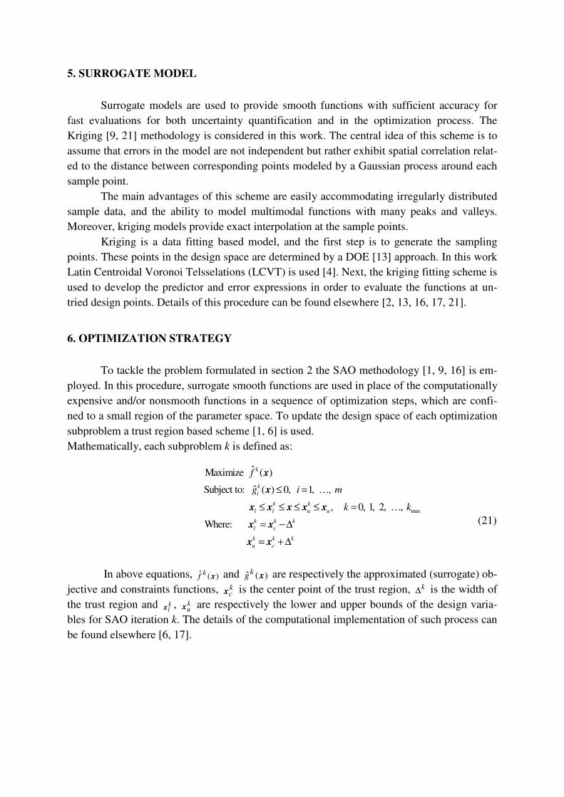
Figure 1 presents a diagram of the methodology layered and nested, according to the

scheme: Sut are the responses of the objective function in the surrogate model, u is the sto-

chastic state variable (for example, the permeability field), e ru is the response of high-fidelity

model (simulator), Su is the objective, for example, the expected NPV, d are the control

variables, which in this work are the liquid rates in production wells.

Figure 1. Layered and Nested Methodology.

With this methodology it is possible to perform optimization studies in oil reservoirs, where

the gradients of the problem are not available or require high computational resources to be

obtained, in addition, uncertainties in petrophysical properties are considered.

The following is a summary of the optimization under uncertainty process applied in

this work:

1. A number of well rate samples are obtained in the trust region by the LCVT method [4].

2. For each sample an uncertainty quantification process is developed, and the expected

NPV is obtained.

3. A surrogate model is generated in the trust region.

4. An optimization process using sequential quadratic programming is developed in the

surrogate model.

5. The response in the high-fidelity model is calculated using optimal control variables

found in step 4.

6. The convergence of the process is verified.

7. The trust region is modified, according to a comparison between values of the high-

fidelity model and the surrogate model.

8. Return to step 1.

8. EXAMPLE

The case study presented here is a waterflooding problem in oil reservoir with one

injection and two production wells, as illustrated in Figure 2. The reservoir has an area of 510

x 510 m2, with a thickness of 4 m and is modeled with a mesh 51x51x1. 1000 possible

realizations for the permeability field were used. The realizations were generated considering

the following covariance function [10]:

( ) ( )1 2 1 2

1 2cov

x x y y

b b

Eeσ

− −− −

= (22)

In the above equation (x1,y1) , (x2,y2) are the coordinates of two generic points on the grid, b1 e

b2 are correlation length and σE is the standard deviation. The following values are attributed

for the studies: b1= 6 , b2= 9 and σE = 1.

Figure 2. Reservoir model.

The production time for the reservoir is 24 years. The two producers wells are part of a

platform system operating with a liquid flow of 6 m3/day. The objective function of

optimization problem is the NPV (Eq. (4)), and the design variables are the liquid rate at

producers that have limits of 25% and 75%. Two control cycles of production time are used,

the first and second ranges were 8 years and 16 years respectively, this implies two design

variables problem. Initially a deterministic optimization study was conducted, where one of

the possible realizations was chosen (Figure 3).

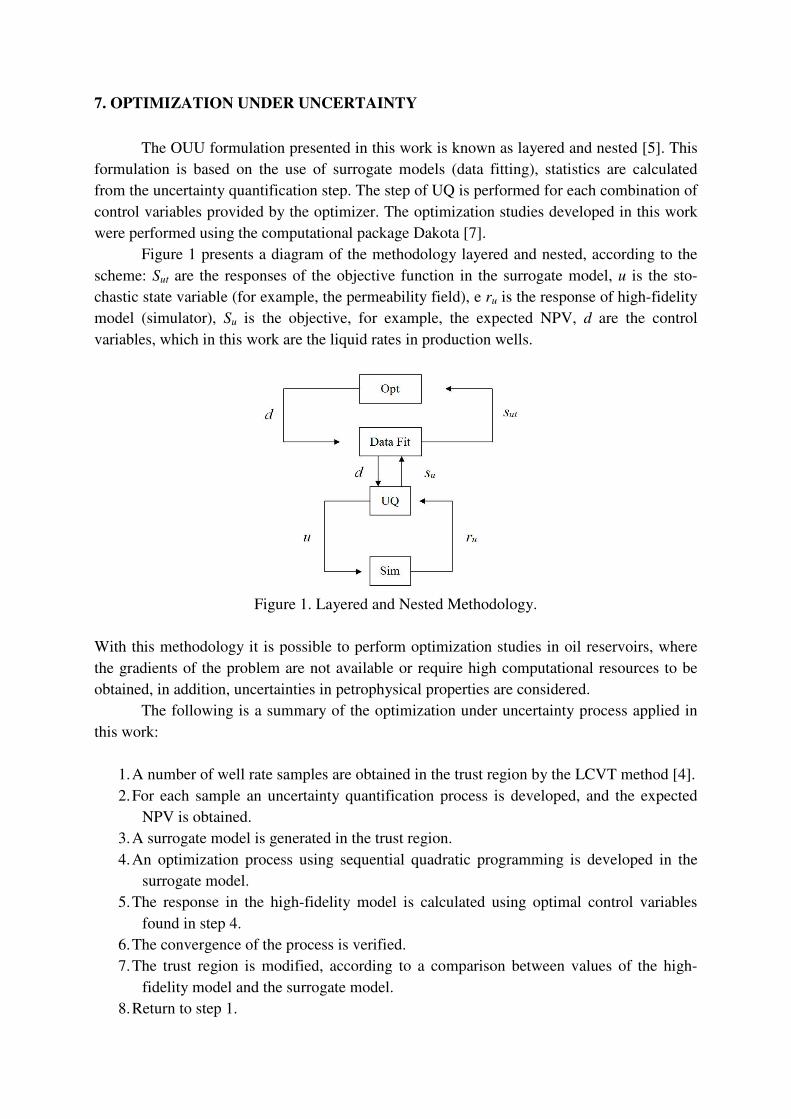
Figure 3. Realization chosen for the study of deterministic optimization.

The deterministic optimization was performed with SAO strategy, where kriging

surrogate models were used in the trust regions. The models were constructed with LCVT

sampling. Table 1 presents the results of deterministic optimization. The Table shows that the

NPV is maximum when the well 1 operates with a 26.4% in the first interval of time (eight

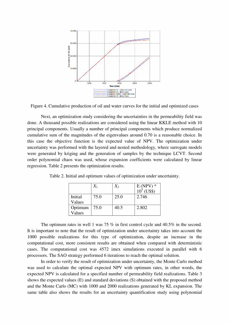
years) and 70.7% in the second interval (16 years remaining). Figure 4 shows the cumulative

production of oil and water curves for the initial and optimized cases.

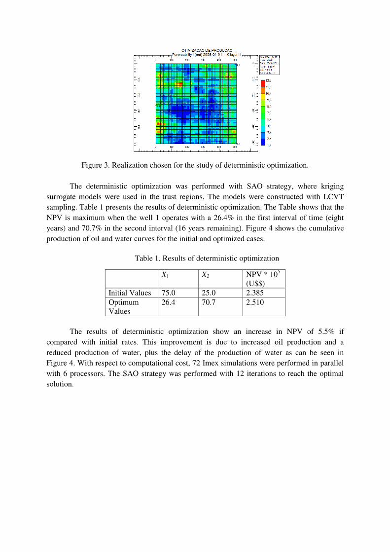
Table 1. Results of deterministic optimization

X1 X2 NPV * 105 (U$$)

Initial Values 75.0 25.0 2.385

Optimum Values

26.4 70.7 2.510

The results of deterministic optimization show an increase in NPV of 5.5% if

compared with initial rates. This improvement is due to increased oil production and a

reduced production of water, plus the delay of the production of water as can be seen in

Figure 4. With respect to computational cost, 72 Imex simulations were performed in parallel

with 6 processors. The SAO strategy was performed with 12 iterations to reach the optimal

solution.

Figure 4. Cumulative production of oil and water curves for the initial and optimized cases

Next, an optimization study considering the uncertainties in the permeability field was

done. A thousand possible realizations are considered using the linear KKLE method with 10

principal components. Usually a number of principal components which produce normalized

cumulative sum of the magnitudes of the eigenvalues around 0.70 is a reasonable choice. In

this case the objective function is the expected value of NPV. The optimization under

uncertainty was performed with the layered and nested methodology, where surrogate models

were generated by kriging and the generation of samples by the technique LCVT. Second

order polynomial chaos was used, whose expansion coefficients were calculated by linear

regression. Table 2 presents the optimization results.

Table 2. Initial and optimum values of optimization under uncertainty.

X1 X2 E (NPV) * 105 (U$$)

Initial Values

75.0 25.0 2.746

Optimum Values

75.0 40.5 2.802

The optimum rates in well 1 was 75 % in first control cycle and 40.5% in the second.

It is important to note that the result of optimization under uncertainty takes into account the

1000 possible realizations for this type of optimization, despite an increase in the

computational cost, more consistent results are obtained when compared with deterministic

cases. The computational cost was 4572 imex simulations executed in parallel with 6

processors. The SAO strategy performed 6 iterations to reach the optimal solution.

In order to verify the result of optimization under uncertainty, the Monte Carlo method

was used to calculate the optimal expected NPV with optimum rates, in other words, the

expected NPV is calculated for a specified number of permeability field realizations. Table 3

shows the expected values (E) and standard deviations (S) obtained with the proposed method

and the Monte Carlo (MC) with 1000 and 2000 realizations generated by KL expansion. The

same table also shows the results for an uncertainty quantification study using polynomial

chaos expansion (PCE), which can be verified the accuracy of polynomial expansion (132

simulations) compared to the Monte Carlo method (1000 and 2000 simulations). These results

are obtained for the optimal rates in the process of optimization under uncertainty.

Table 3. Expected value and standard deviation of NPV for uncertainty quantification studies.

PCE MC – 1000 MC – 2000

E (NPV) * 105

(U$$)

2.802 2.796 2.793

S (NPV) * 105

(U$$)

0.201 0.196 0.202

The expected NPV and the standard deviation obtained show the accuracy of the

polynomial chaos expansion when compared with the Monte Carlo method (Table 3). It is

important to emphasize that in the PCE 132 simulations performed in the high-fidelity model

were necessary, whereas the Monte Carlo method required respectively 1000 and 2000

simulations.

A study to verify the robustness of the optimization under uncertainty solution was

performed [23]. Four realizations of 1000 possible were randomly chosen. For each

realization a deterministic optimization study was run. Then, the optimal rates obtained in the

process of optimization under uncertainty were assigned to each of the four realizations and

then the NPV was calculated. In the final step the optimal deterministic rates obtained in each

of the four realizations were allocated to the other three realizations in the study. For example,

the optimal rates obtained in the realization 1 were allocated in the reservoir considering the

realization 2, 3 and 4. This process was repeated for all realizations, and the NPV was calcula-

ted for each case. Tables 4 and 5 present all the results of the robustness verification process.

Table 4 shows the results obtained for the deterministic optimization process for each chosen

realization, as well as the results obtained in the optimization under uncertainty study. In

Table 5, the letter R represents a realization. In bold, the results obtained in the deterministic

optimization process. Figure 5 shows the results of Table 5 in a graph form, in order to clarify

the results.

Table 4. Flows rates and NPV results for the deterministic optimization and OUU process.

Realization 1

(C1 Case)

Realization 2

(C2 Case)

Realization 3

(C3 Case)

Realization 4

(C4 Case)

Rates (%) [0.26, 0.70] [0.25, 0.75] [0.67, 0.59] [0.72, 0.31]

NPV *

105 (U$$)

2.510 2.964 3.059 2.902

Table 5. Results for robustness of the optimization under uncertainty process.

R 1 R 2 R 3 R 4 Mean Value

NPV OUU Case

* 105 (U$$)

2.460 2.850 2.990 2.877 2.794

NPV C1 Case

* 105 (U$$)

2.510 2.506 3.058 2.664 2.685

NPV C2 Case

* 105 (U$$)

2.385 2.964 2.802 2.893 2.761

NPV C3 Case

* 105 (U$$)

2.476 2.594 3.059 2.728 2.714

NPV C4 Case

* 105 (U$$)

2.418 2.935 2.888 2.902 2.786

Figure 5. Graph of NPV results shown in Table 5.

The results presented in Tables 3 to 5, and also in Figure 5 represent the robustness of

the result obtained in the optimization under uncertainty process. As expected, the NPV

values related to deterministic optimization are the best cases for each realization. However,

in the real reservoir problems true realization of the permeability field is not known,

invalidating the deterministic optimization. The NPV values obtained with the rates coming

from optimization under uncertainty (OUU) are good, especially when compared with results

obtained from the rates resulting from the deterministic optimization process performed in

each realization.

The rates obtained in the process of optimization under uncertainty, when placed in

each of the four selected realizations, producing a mean NPV of 2794 x 105 U$$. This value

is higher than the mean NPV values obtained where C1, C2, C3 and C4 using the controls

rates of other realizations (Table 5). The optimal rate obtained in the optimization process

under uncertainty in each case produce a satisfactory estimate of the NPV. The OUU method

used prevents the worst cases of control to be chosen. This would happen, for example, if

deterministic optimization of the rates were calculated on the realization 2 and the real

reservoir realization was realization 1, as shown in Figure 5. In this situation, the resulting

NPV from realization 1 would be lower when compared to the NPV produced by OUU

process. This same idea can be applied to the realization 2, 3 and 4 (Figure 5).

9. CONCLUSIONS

The main conclusions of this work are presented below:

1. The use of surrogate models is a computationally feasible alternative for solving

optimization problems in oil reservoir where the gradients of the problem are not

available or will require high computational resources to be obtained. It is important to

note that feasibility of the optimization under uncertainty problems depends on the use

of parallel computation.

2. The use of the polynomial chaos expansion proved to be efficient compared with the

Monte Carlo technique.

3. The optimization under uncertainty procedure presented robust results, that is, the

control rates obtained in the process had certain immunity to the lack of knowledge of

the real permeability field.

ACKNOWLEDGMENT

The authors acknowledge the financial support for this research given by ANP (Nation-

al Agency of Petroleum, Brazil), CNPQ and PETROBRAS.

REFERENCES

[1] Alexandrov, N., Dennis Jr., J.E., Lewisand, R.M. and Torezon, V. “A Trust Region

Framework for Managing the Use of Approximation Models in Optimization”,

NASA/CR-201745; ICASE Report No. 97-50, 1997.

[2] Afonso, S. M., Horowitz, B., Lira Junior, J. D., Carmo,, A., Cunha, J., Willmerdorf, R.

Comparison of Surrogate Building Techniques for Engineering Problems. XXIX Cilam-

ce, 2008.

[3] Cmg - Computer ModelLing Group Ltd, “Imex - User´s Guide”, 2006.

[4] Du, Q., Vance, F., Gunzburguer; M. Centroidal Voronoi Tessellations: Applications and

Algorithms, Society for Industrial and Applied Mathematics, 1999.

[5] Eldred, M.S, Giunta, A. A., Wojtkiewicz, J., Trucano, T. G. Formulations for Surrogate-

Based Optimization under Uncertainty. AIAA Paper 2002-5585, 2002.

[6] Eldred, M.S., Giunta, A.A. and Collis, S.S. “Second-Order Corrections for Surrogate-

Based Optimization with Model Hierarchies”, Paper AIAA-2004-4457 in Proceedings of

the 10th AIAA/ISSMO Multidisciplinary Analysis and Optimization Conference, Albany,

NY, 2004.

[7] Eldred, M. S., et al., “Dakota - User´s Manual”, 2008.

[8] Eldred, M. S., Webster, C. G. Evaluation of non-Intrusive Approaches for Winer- Askey

Generalized Polynomial Chaos. AIAA Paper 2008-1892, 2008.

[9] Forrester, I. J., Sobester, A., Keane, A. J. Engineering Design via Surrogate Modeling,

John Wiley and Sons, 2008.

[10] Ghanem, R., “Probabilistic Characterization of Transport in Heterogeneous Media”.

Computer Methods in Applied Mechanics and Engineering, Elservier, 158 199-220, 1998.

[11] Giunta, A.A., Watson, L.T. A Comparison of Approximation Modeling Techniques:

Polynomial versus Interpolating Models. Paper AIAA-98-4758 in proceedings of 7th AI-

AA/USAF/NASA/ISSMO Symposium on Multidisciplinary Analysis & Optimization, St.

Louis, MI, 1998.

[12] Giunta, A. A., Eldred, M. S. Implementation of a Trust Region Model Management

Strategy in The Dakota Optimization Toolkit, AIAA-2000-4935, 2000.

[13] Giunta,, A. A., Use of Data Sampling, Surrogate Models, and Numerical Optimization

in Engineering Design, Proceedings of the 40th AIAA Aerospace Sciences Meeting and

Exhibit, Reno, NV, 2002.

[14] Huang, S. P., Quek, S. T., Phoon, K. K. Convergence study of the truncated Karhunen–

Loeve expansion for simulation of stochastic processes. International Journal for Numeri-

cal Methods in Engineering. 52:1029–1043, 2001.

[15] Jones, D. R., Schonlau, M., Welch, W. J. Efficient Global Optimization of Expensive

Black-Box Functions. Kluwer Acadmeic Publishers, 1998.

[16] Keane, A.J., Nair, P.B., Computational Approaches for Aerospace Design: The Pursuit

of Excellence, John-Wiley and Sons, 2005.

[17] Lira Jr, J. D. Otimização com Modelos Substitutos Considerando Incertezas em Reser-

vatório de Petróleo. Phd Thesis, Civil Engineering, UFPE, Brazil, 2012.

[18] Oliveira, D.F.B., Técnicas de Otimização da Produção para Reservatórios de Petróleo:

Abordagens Sem Uso de Derivadas para Alocação Dinâmica das Vazões de Produção e

Injeção. Master Thesis, Civil Engineering, UFPE, Brasil, 2006.

[19] Sarma, P., Durlosfky, L. J., Aziz, K., “Kernel Principal Component Analysis for Effici-

ent Differentiable Parameterization of Multipoint Geostatistics”. Math Geosci 40:3-32,

2008.

[20] Scholkopf, B., Smola, A, Muller K., “Nonlinear Component Analysis as a Kernel Ei-

genvalue Problem”, Technical Report No. 44, Max-Planck Institut für biologische Kyber-

netik, Arbeitsgruppe Bülthoff, 1996.

[21] Simpson, T. W, Maurey, T.M , Korte, J.K , Mistree, F. “Kriging Models for Global

Approximations in simulation-Based Multidisciplinary Design Optimization” , AIAA

Journal, 39(12), 2233-2241, 2001.

[22] Tatang, M. Direct Incorporation of Uncertainty in Chemical and Environmental Engine-

ring Systems. Phd Thesis, MIT, 1995.

[23] Van Essen, G.M., Zandvliet, M. J., Van Den Hof, P. M. J., Bosgra, O. H. Robust Water-

flooding Optimization of Multiple Geological Scenarios, SPE 102913, SPE Journal, 2006.

[24] Xiu, D., Karniads, G. Modeling Uncertainty in Flow Simulation via Generalized Poly-

nomial Chaos. Journal of Computational Physics 187 137-167, 2003.