Watertight Surface Reconstruction for Uncertain Data

Watertight Surface Reconstruction for Uncertain Data

Markus Wiedemann

Dru

cksa

chen

kate

go

rie

Watertight Surface

Reconstruction for Uncertain

Data

eingereichte

MASTERARBEITvon

cand. ing. Markus Wiedemann

geb. am 27.07.1988

wohnhaft in:Lechstraße 10

86931 PrittrichingTel.: 0172 8557139

Lehrstuhl furINFORMATIONSTECHNISCHE REGELUNG

Technische Universitat Munchen

Univ.-Prof. Dr.-Ing. Sandra Hirche

Betreuer: Dipl.-Ing. Simon Kriegel (DLR), Dr.-Ing. M. LeiboldBeginn: 01.05.2014Zwischenbericht: 15.08.2014Abgabe: 02.12.2014

In your final hardback copy, replace this page with the signed exercise sheet.

Abstract

For simple pick and place tasks, a robot needs to be able to recognise objects. Inorder to avoid scanning all objects by hand, an automatic modelling approach is nec-essary. Considering space and price restrictions on a robotic platform, the quality ofperceiving devices suffers from this restrictions. Consequently modelling approachesneed to cope with pose errors and noisy data that usually result in displaced surfacesincorporating a lot of artefacts.In this work, we focus on creating a watertight surface representation that is auto-matically built by a robot. Therefore, we develop a next best viewpoint planningmethod that fits to an afterwards applied filtering stage for improving measurementconfidence. Using the resulting data, a mesh growing approach reconstructs thesurface of the to be scanned object incorporating an inflating and a detailing stage.Our approach is able to roughly estimate the objects surfaces using inaccurate hard-ware and even to reconstruct small details for precise laser scanning devices. Smallareas that are not scanned can be filled and highlighted by utilizing the near neigh-bourhood of measurements.

Zusammenfassung

Damit Hol-und-Bring Aufgaben ausgefhrt werden knnen, muss ein Roboter diezu bringenden Objekte erkennen. Um zu vermeiden, dass all dieses Objekte perHand eingescannt werden, ist eine Applikation notwendig, die dies automatischdurchfhrt. Durch beschrnktes Platzangebot und einen eingeschrnkten Kostenrah-men einer robotischen Plattform leidet die Qualitt und Genauigkeit von optischenMessgerten.Das fhrt dazu, das Modell bildende Anstze Fehler in Pose und verrauschte Daten, diezu versetzten und mit Artefakten besetzten Oberflchen fhren, beachten mssen. Indieser Arbeit konzentrieren wir uns auf einen Ansatz, der eine wasserdichte Ober-flchenreprsentation automatisch mithilfe eines Roboters erstellt. Dafr entwickelnwir zunchst eine Planungsphase, die den nchste Scanpunkt generiert und dabei dieAnforderungen der darauf folgenden Filterphase erfllt. Die gefilterten Daten werdendann von einem Ansatz benutzt, der ein Gitternetz wachsen lsst, das die Oberflcheeines zu scannenden Objektes darstellt. Jener besteht aus einer Inflations- und einerDetaillierungsphase.Unsere Applikation ermglicht im Angesicht von ungenauer Hardware eine grobeSchtzung von Oberflchen und bei Benutzung von hoch przisen Laser Scannern, sogardie Rekonstruktion von kleinen Details. Kleine Bereiche, die gescannt wurden, kn-nen hervorgehoben und rekonstruiert werden, indem rtlich nahe liegende Messungenbenutzt werden.

2

CONTENTS 3

Contents

1 Introduction 5

1.1 Problem Statement . . . . . . . . . . . . . . . . . . . . . . . . . . . . 51.2 Related Work . . . . . . . . . . . . . . . . . . . . . . . . . . . . . . . 5

1.2.1 Next Best View Planning . . . . . . . . . . . . . . . . . . . . 61.2.2 Iterative Closest Point . . . . . . . . . . . . . . . . . . . . . . 71.2.3 Surface Reconstruction using Deformable Meshes . . . . . . . 11

2 Methods 17

2.1 Volumetric Discretisation . . . . . . . . . . . . . . . . . . . . . . . . . 172.2 Scanning . . . . . . . . . . . . . . . . . . . . . . . . . . . . . . . . . . 19

2.2.1 Next Best View Planning . . . . . . . . . . . . . . . . . . . . 192.3 Preprocessing . . . . . . . . . . . . . . . . . . . . . . . . . . . . . . . 21

2.3.1 Registration . . . . . . . . . . . . . . . . . . . . . . . . . . . . 212.3.2 Filtering . . . . . . . . . . . . . . . . . . . . . . . . . . . . . . 21

2.4 Surface Reconstruction . . . . . . . . . . . . . . . . . . . . . . . . . . 222.4.1 Inflating Stage . . . . . . . . . . . . . . . . . . . . . . . . . . 232.4.2 Detailing . . . . . . . . . . . . . . . . . . . . . . . . . . . . . . 262.4.3 Smoothing and Regularizing . . . . . . . . . . . . . . . . . . . 27

3 Experimental Results 31

3.1 Viewplanning . . . . . . . . . . . . . . . . . . . . . . . . . . . . . . . 363.2 Registration . . . . . . . . . . . . . . . . . . . . . . . . . . . . . . . . 393.3 Filtering . . . . . . . . . . . . . . . . . . . . . . . . . . . . . . . . . . 423.4 Surface Reconstruction . . . . . . . . . . . . . . . . . . . . . . . . . . 473.5 Laser Scanned Objects . . . . . . . . . . . . . . . . . . . . . . . . . . 52

4 Conclusion and Outlook 55

List of Figures 59

List of Abbreviations 61

Bibliography 63

4 CONTENTS

5

Chapter 1

Introduction

In recent years, the field of human assisting service robots is getting more andmore attention in robotic research. For robots assisting humans, it is necessary toenable them to perceive their environment and create a computer understandablerepresentation of it. This work focuses on the generation of a mesh based on scandata utilizing a mobile robot equipped with a manipulator, to scan given objectsand create a mesh representation of them.

1.1 Problem Statement

For scanning objects, a variety of sensors exist that scan the distance to a surface.Examples for this are laser stripers that come with a high price but have the ad-vantage of precise measurement. In comparison to that, another popular and cheapexample is Microsoft’s Kinect camera. However, it is not able to reach the accuracyof a laser striper. For creating mesh representations, those drawbacks have to bekept in mind.Due to discretisation and measuring failures, a straight forward meshing algorithmwould produce discontinuous and self-intersecting representations of real world ob-jects. A further error occurs hand in hand with a position tracking device. Thiscan be cameras in combinations with markers or a manipulator that either holdsan object or a camera mounted to it. Those pose errors lead to displaced pointclouds and therefore failures in the depth perception. Another source of error arereflections by translucent media. They induce further errors in the measured depth.Consequently, appropriate methods have to be found and implemented to cope withuncertainties of 3D perception.

1.2 Related Work

For surface reconstruction it is first necessary to plan the scanning of an unknownobject. Therefore, viewpoints need to be generated. This means the position and

6 CHAPTER 1. INTRODUCTION

the viewing direction of a scanning device need to be calculated. Related work onplanning the next best view will be introduced in the succeeding subsection. Afterscanning, an automatic algorithm is expected to cope with errors in orientation andposition of the scanning device. Considering those errors to be only small in the givenscenario, we will take a closer look at the Iterative Closest Point (ICP) algorithm.Finally, we introduce the basic concept of deformable surface reconstruction thataims at building a mesh consisting of triangles in order to represent the surface ofthe scanned object.

1.2.1 Next Best View Planning

The first step in scanning real world objects is to plan the Next Best View (NBV).Here, suitable positions and view directions of the scanning device have to be gen-erated and evaluated with respect to their information gain. There exists a varietyof solutions for this problem. Lamp et al. [1] implemented an automatic scanningsystem where five strategies are implemented that are described as follows:

Edge-Scan Edges are defined as being the connecting between two faces with dif-ferent normals. The scan is oriented towards the negative mean of the twonormals and follows the edge.

Raster-Scan Here, the scan is directed on a planar surface and oriented along itsnegative normal.

Box-Scan For the Box-Scan, the scan performs the Edge-Scan and a Raster-Scanon a the top edges and five faces of a virtual box.

Profile-Scan Using a previously performed scan, here the scanner follows the con-tour of a raw model.

Servo-in-Depth Here, the scanner’s trajectory follows the contour of the modelby using online the already scanned surface.

The authors aimed at implementing a semi-automatic scanning software where theuser decides which scan strategy is to be used.A further strategy based on a mesh model was introduced by Khalfaoui et al. [2].They calculate the Mass Vector Sum (MVS) - introduced by Loriot et al. [3] - byadding up the surface normals of the boundary patches of the model. View pointcandidates are produced by utilizing the surface normals of nearby surfaces of theMVS. For each view point candidate k, a weight in timestep i is calculated by

wik =

θikθimax

where θimax is the maximum difference angle and θik the difference angle of the cur-rent viewpoint direction to the MVS. All viewpoints are then grouped in clusters,

1.2. RELATED WORK 7

the average weight for each cluster is calculated and the cluster with the highestaverage weight is chosen as next best view point.Massios and Fisher [4] generate viewpoints on a sphere around the to be scannedobject. They first filter the viewpoints with respect to their reachability due tokinematic restrictions of the robot. The remaining viewpoints then are evaluated ona voxelspace by a visibility and a quality criteria. The visibility criteria representsthe number of visible voxels that were occluded in previous scans. For the qualitycriteria all previously scanned voxels are used. The quality qi of each voxel is esti-mated for each performed scan and used for the next. It is calculated by averagingthe normals of all surfaces inside this voxel and calculating the dot product of theaverage normal and the viewing direction. The quality of a voxel is only changed,if the current scan’s quality is higher than the previous ones. This quality is thenused for calculating a further quality value fquality for a simulated scan that scansthe set of M voxels:

fquality =1

|M |

(

M∑

i=1

(1− qi)(|v · ni)

)

where v is the viewing direction and ni the average normal of voxel i. Both criteriaare multiplied by individual weights and then added up to a total quality estimationvalue.Kriegel et al. [5] estimate the curvature of the boundaries of the mesh model. Basedon that viewpoints are generated perpendicular to the estimated curvature. Theyintroduce in [6] a quality criteria for determining the next best view point. Therefore,the authors estimate the total information gain by performing a simulated scan foreach viewpoint. Using a voxelspace whose states describe the probability p of a voxelbeing occupied, for each by the simulated scan intersected voxel a entropy Hvoxel iscalculated as

Hvoxel = −p log(p)− (1− p) log(1− p).

By adding up Hvoxel for all intersected voxels, the information gain for a certainviewpoint can be estimated. Furthermore, they introduce in [7] an additional criteriafor determining the next best view. They estimate the quality qi of a surface patchof the voxel i by incorporating the point density di of that voxel and the proportionof boundaries inside it relative to the total number of boundaries bi:

qi = λ · bi + (1− λ) · di.

Here, λ is a user defined parameter for weighting the two criteria. Furthermore, ifthe average normal of all surfaces inside the voxel differs more than 70◦ from theviewing direction, qi is set to zero for that voxel.

1.2.2 Iterative Closest Point

In recent past, many different variants of the ICP algorithm were published. The firstversions were introduced by Chen and Medioni [8]in 1991 and Besl and McKay [9]


in 1992.The main idea of ICP is to iteratively minimise the distance between two pointclouds. Therefore, we first define one as the reference cloud which is fixed to itspose. The second cloud is iteratively aligned to the reference cloud and we referto it as data cloud in the following. The variants of ICP differ in several aspects,therefore we structure the key points in the succeeding section in the style of [10].

Selection

For choosing which points of the data cloud to use multiple possibilities exist. Chenand Medioni [8] suggest to use regularly distributed points that are in a ”smoothneighbourhood”. In order to check this, the authors suggest to fit a smooth surfacefunction, e.g. a plane, to the neighbourhood by using least squares and afterwardsevaluating the standard deviation.Besl and McKay [9] use all points of the data cloud. In contrast, Toldo et al. [11]use only those points of the data cloud that are the mutually closest points. Thismeans, that we search in the reference cloud the closest points to every point of thedata cloud. Mutually closest is, if this is as well vice versa.Masuda et al. [12] use random sampling on the data cloud. Zhang [13] as well asNeugebauer [14] propose to use only a small number of points that are uniformlydistributed until a certain convergence criterion is fulfilled. Then more and morepoints are included until all points are used. Neugebauer [14] supposes a speed-upfactor of 20− 100. A dynamical selection of points was proposed by Chetverikov etal. [15]. They suppose to calculate the distances between each point pair and sortingthem with respect to their distance. Then only a fixed number of them representingthe smallest distances are used.

Correspondences

In order for aligning points to the data cloud, we need to select corresponding pointsin the reference cloud.

Point to Point Besl and McKay [9] use the closest point of the reference cloud foreach point of the data cloud.Using a k-d-tree can significantly accelerate this search as proposed by Si-mon [16].

Closest Line Another possibility was introduced in 2008 by Censi [17] that utilizesthe point to line distance. For each point of the data cloud the closest twopoints of the reference cloud have to be found. Then the distance between thefirst point and the connecting line of the latter two points is minimized. Thisapproach was introduced only for 2D data.

1.2. RELATED WORK 9

Point to Plane The chronologically first published correspondence selection ap-proach is the point to plane projection introduced by Chen and Medioni [8].It follows the work of Potesil [18] by using the surface normal of the selectedpoint of the data cloud and intersecting it with the reference cloud. Therefore,the points of the reference cloud are approximated using planes and then theintersection of the surface normal with these planes are calculated.Another possibility for the point to plane approach is to project the points ofthe data cloud onto the reference cloud in the direction of the camera view.This means that we first transform the data cloud in the coordinate systemof the reference cloud. Then the depth value is adjusted to be aligned to thereference clouds surface. Afterwards, we search the nearest point on this sur-face. This idea was introduced in 1997 by Neugebauer [14].Masuda et al. [12] use the point-to-triangle distance which is closely related tothe point to plane distance. They as well optimise the search for the nearesttriangle with the use of a k-d-tree.

There exist other possibilities to find correspondences, e.g. based on colour or lightintensity which we do not list here, as we solely concentrate on the given depthinformation.

Correspondence Weighting

Once correspondences are found, we can weight them in different ways. The firsttwo approaches by Besl and McKay as well as Chen and Medioni do not include anyweighting strategies and therefore, this can be seen as using a constant weight of 1.Rusinkiewicz [10] considers using weighting based on the point-to-point distance forthe correspondences. Here, points that are farther away from their correspondencesget lower weights and vice versa. Another possibility examined by Rusinkiewicz andLevoy is to use the ”compability of normals” expressed by

Weight = n1 · n2

as well as to use the expected noise produced by the scanning device. This errormetric is highly dependent on the used hardware and examples for different noisemodels utilized for depth measuring devices can be found in [19, chap. 3], [20] or [21].Toldo et al. propose to compute the ”Median of Absolute Deviations” MAD [11]and use its inverse value, meaning 1−MAD.A further method was introduced in 2009 by Segal et al. [22]. They propose to use theproperty that a real world object has to be at least locally planar. Consequently, theprobability distribution along the normal of a point coincides with the uncertaintyof the measuring device. In the directions orthogonal to the normal the uncertaintyshould become bigger and therefore, the main movement of a point while registeringshould be applied to this directions.


Point Rejection

As the hardware used for obtaining point clouds are bound to noise and uncertain-ties, we have to consider the possibility of outliers. This means that there are pointsgenerated due to reflections or other sources of error. We need an efficient approachto deal with those outliers. Turk and Levoy [23] use a fixed threshold to discardoutliers. Pandey et al. [24] define this threshold to be dynamically calculated. Thisis done by estimating the camera motion and restricting the correspondence searchto a local region. Furthermore, Turk and Levoy discard correspondences that lie ona boundary of a mesh. Considering a surface meshed according to the techniquespresented in sec. 1.2.3, if this surface ends somewhere, the points on this ending arenot allowed to be correspondences for the ICP algorithm.Masuda et al. [12] use a classification algorithm to determine whether the pointsof the data clouds are ”inliers” or ”outliers”. Therefore, they check if the distancebetween points of the data cloud to the meshed model are within a threshold. Ifthey are, they are inliers and are used for further calculation. This step is repeatedin every iteration and therefore, inliers can become outliers and vice versa during thealgorithm. The threshold used by Masuda et al. is 2.5 times the standard deviation.A similar approach is used by Zhang [13] but with a small deviation. His threshold isbased on the relation between the old threshold and the current standard deviationand a first threshold has to be set by the user.Pulli [25] suggests using multiple conditions. The first condition is to use only pointpairs if their normals do not differ more than 45◦. As second, the authors integratedthe idea of Turk and Levoy [23] where points on the mesh boundaries are rejected.Furthermore, only a percentage of the closest point pairs are considered and there-fore all other points are rejected. Additionally, correspondence pairs whose distanceis greater than a certain threshold are rejected as well. The remaining pairs areupdated in every step.Using these techniques, there exists a variety of ICP algorithms. A small numberof some of these variants or its derivatives can be found in [8–12, 15, 22, 24–27] andothers.

1.2. RELATED WORK 11

1.2.3 Surface Reconstruction using Deformable Meshes

Using 2.5D cameras comes with the price of noisy data. However, for being ableto reconstruct detailed surface representations of real world objects, we want toimplement a deformable meshing algorithm. The advantages of this are that morethan one scan can be integrated in a mesh and outliers or noisy data can be correctedby new measurements. We hope to be able to improve scanning, even though cheaperand consequently lower quality devices are utilized for perception.The idea of deformable entities was first introduced by Kass et al. [28] in 1988. Theydescribed snakes as splines that are attracted to significant image features such asedges. This framework is designed to integrate user input as initial positions of thesnakes, applying pushing forces to move them out of local minima and moving themsmoothly with a spring dynamic. Their inner dynamic is constantly minimizing itsenergy and therefore is even able to track moving edges in intensity images.Miller et al. [29] based on this idea a framework for extracting topology closedmodels for 3D data. They extended the snake approach for the use of 3D polygonsin order to reconstruct meshes of real objects. In order to do so, they use a seedmodel as initial configuration, which is then expanded until the surface of an objectis reached.A further extension was introduced in 1992 by Vasilescu and Terzopoulos [30]. Intheir approach, a discontinuity detection was implemented which in case of founddiscontinuities could subdivide polygons, and merge them if necessary.The next step towards state of the art deformable meshes was published in 1998 byLachaud and Montanvert [31]. They introduced a generic approach that allowed toconstruct and deform a mesh in different resolutions. This means, their frameworkstarts with a low resolution in order to build a coarse model of the object. In thefurther proceeding, the coarse model is refined by dividing the triangles iterativelyup to the desired resolution or edge length. With this framework, the first selfcollision scheme was introduced. Here, not neighbouring triangles whose distance isbelow a certain threshold start a melting process between the two parts of the mesh.In the following, we will give a brief description of the different node dynamics andthe subdividing and merging approaches that characterize the aforementioned andfurther publications.

Energy Based Expansion

The basic approach for the expansion strategy is to use a combination of internaland external forces in an mass-damper-spring system for an element i:

mixi + rixi + gi = fi.

Here, mi represents the mass, ri a damping coefficient, gi the sum of internal andfi the sum of external forces. x and its first and second derivatives x and x are theposition, velocity and acceleration of the element i respectively.


Internal Forces As internal forces, a variety of authors, e.g. [30–33], use a com-bination of two forces: The spring force and a bending force. The spring forcecan be interpreted as a force that spreads a deformation of one vertex xi onto itsneighbourhood and can be expressed with

fs,i =∑

j∈N (xi)

(

cij||xj − xi|| − lij

||xj − xi||xj − xi

)

,

where cij is the stiffness between node i and j, N (xi) represents the set of neigh-bouring nodes of i and lij the natural length of the spring between node i and nodej.The second internal force, the bending force, helps to smooth the curvature of thesurface represented by the triangulated mesh. It is calculated as

fb,i = c(xi)− xi −1

n(xi)

∑

j∈N (xi)

(c(xij)− xij)

with n(xi) being the number of neighbours, xij = xj − xi and c(xi) the barycenterof the neighbours of node i that can be calculated as

c(xi) =1

n(xi)

∑

j∈N (xi)

xij .

Both forces are summed up and weighted by user defined parameters ws and wb andgive the internal force gi for node i

gi = wsfsi + wbfb,i.

External Forces A common approach for computing external forces is to use twodifferent forces:

• inflation force

• edge force.

Here, the inflation force is implemented in order to assure the growth/shrinking ofthe seed model until a possible boundary of the object is reached. Therefore, thisforce is directed in direction of the normal of a vertex or triangle and simply pushesthe mesh until a voxel is reached in which the boundary could lie.Chen and Medioni [33] determine the maximal possible spring force and adapt thescalar value k of the inflation force to be greater.Park et al. [32] suggest to apply two user defined lower and upper thresholds Tlow

and Thigh:

k =

{

+1 Tlow ≤ I(xi) ≤ Thigh

−1 else.


Lachaud and Montanvert compute a continuous scalar field Π(x) of the volumetricimage by tri-linear interpolation and calculate the inflation force by evaluating

k = α (Π(xd)− Π(xi))

with Π(xd) being the value of a desired iso-potential surface and α a user specifiedweighting factor.

For the edge force the gradient of the volumetric image is used for pushing themesh towards local minima or maxima. For computing the gradient, Lachaud andMontanvert [34] use the Sobel operator and produce a continuous vector field by tri-linear interpolation. Park et al. [32] use the 3D Monga-Deriche edge-detector [35]to produce a intensity edge field and afterwards tri-linear interpolate using the eightsurrounding voxels to compute the gradient field.

Dynamical Topology

In order not to rely on the number of vertices and triangles of the seed model,different approaches for splitting triangles and merging them have been proposed.

Merging Triangles Lachaud and Montanvert [34] introduced the concept ofmerging two parts of a mesh if their distance is below a certain threshold. There-fore, they first create intermediate points between those parts and then triangulatebetween those two parts. Chen and Medioni [33] search for long and thin trianglesand switch the shared edge in order to create two better posed triangles. Fig. 1.1illustrates this issue.

Figure 1.1: Inversion of the shared edge to create better posed triangles

Park et al. [32] search for edges below a certain threshold and merge their verticesas illustrated in fig. 1.2.


Figure 1.2: Merging two vertices whose distance is below a threshold

Splitting Triangles The issue of creating new triangles is more complex thanmerging. The first method for subdividing a triangle was introduced by Vasilescuand Terzopoulos [30]. The basic concept is to cut all three edges and connect thenew constructed vertices as illustrated in fig. 1.3.

Figure 1.3: Splitting a triangle into four smaller triangles

Chen and Medioni [33] implemented a different method. After finding the longestedge in a triangle, this edge is split into two edges. The new vertex is connected tothe to this edge opposing vertex and consequently, two new triangles are constructed.As the split edge is shared with another triangle, this triangle has to be split as well.Chen and Medioni therefore search in this triangle for the longest edge and splitit as well. Successively, this cut has to be propagated to the next triangle. Foran illustration, see fig. 1.4. Here, the upper triangle is split and propagated to theunderlying triangle. This is as well split and further propagated to the lower lefttriangle.


Figure 1.4: Splitting a triangle and propagating it onto the following. The dashedlines represent the propagated cuts.

Lachaud and Montanvert [34] have a similar but simpler approach. Instead of prop-agating the cut up to the next triangles longest edge, they simply cut the sharededge and connect it in both triangles to the opposing vertex. As an illustrationserves fig. 1.5.

Figure 1.5: Splitting a triangle into two smaller triangles


17

Chapter 2

Methods

This chapter introduces a general concept of the scanning algorithm. A key methodfor most of our applications is the so called voxelspace which we briefly describe inthe next section. In fig. 2.1 an overview of the whole scanning algorithm is illus-trated. First the scanning stage is performed. In this stage, each scan is taken andhas to be planned, therefore, the next best viewpoint has to be determined. Thisstage is succeeded by the preprocessing step. Here, the scans are registered andfiltered. As final step, the surface reconstruction is performed with its two stages:inflating and detailing.After introducing the voxelspace, we will look on the scanning process which is fol-lowed by the preprocessing phase. After that we introduce our surface reconstructionalgorithm.

2.1 Volumetric Discretisation

The voxelspace is a commonly used method to efficiently describe volumetric infor-mation. Its concept is to divide a certain space into many small cubes in order todiscretise that space. Each of those cubes represents a small fraction of the givenspace. Further information, such as being occupied or colour can be assigned toeach voxel.An efficient implementation of a voxelspace is the so called octree. Here, the spaceis combined in one big cube. This cube is then split into eight smaller cubes, thatagain can be split into eight further cubes. This procedure is done until a given min-imum edge length is reached. The lastly produced cubes then represent the voxels.Voxels or cubes having the same state can be merged into their parent cube whichleads to an efficient way of storing volumetric information. Furthermore, the treestructure of an octree leads to a fast access rate on the single voxels. An illustrationfor an octree can be found in fig. 2.2.One application for a voxelspace is the creation of maps of the environment forcollision avoidance and path planning [36, 37]. A further application is to use avoxelspace for scanning and building a volumetric representation of rigid objects.

18 CHAPTER 2. METHODS

Scanning

Preprocessing

Surf. Reconstr.

Perform scan

NBV Planning

Registrate scans

Filter scans

Inflating stage

Detailing stage

Figure 2.1: Overview of the scanning and surface reconstruction algorithm

x

yz

0 2 4 6 8

0

1

2

3

4

2

4

6

8

10

12

Figure 2.2: Example for a voxelpace representation using octrees

In both cases through measuring free space, the model or map is carved out of agiven space with unknown state. Additionally, surface information can be insertedinto the voxelspace by setting the state to a value representing occupied volumes.

2.2. SCANNING 19

2.2 Scanning

In order to acquire the necessary measurements, viewpoints need to be generated,meaning poses from where and in which direction the next measurement should beperformed. Therefore, we look onto the key points of our next best view (NBV)planning algorithm in the following subsection.

2.2.1 Next Best View Planning

The NBV stage consists of two steps: First possible next viewpoints are generatedwhich are in the second step evaluated with respect to their simulated informationgain.As our surface reconstruction algorithm differs in various points to the used methodin [6,7] we have different requirements for possible viewpoints. For the filtering stagewe need more than one measurement for each small part of the surface in order toincrease estimation confidence. Consequently, each voxel needs a higher numberof depth points attached to it. This leads to scanning the same part of the to bescanned object more than once.For generating viewpoints, a voxelspace is generated in which five possible statesare present:

Unknown voxels for which no information was gained yet

Free voxels between the camera position and the measured surface

Occupied voxels in which a surface was measured

Possible inside voxels that are behind the measured surface

Possible border voxels that are between unknown and possible inside voxels

For each new scan, this voxelspace is then updated and the given states with excep-tion of the occupied state, can be freely changed to one another. From this spacepossible viewpoint candidates are then generated. Therefore, we form the set B withmagnitude n that consists of all occupied and possible border voxels. For each centerof those voxels bi, i ∈ 1, . . . , n we search for voxels with the state possible insidein a certain neighbourhood and get set Ii of voxels with magnitude m. Using theconnecting vectors dj,i that connect the center of a voxel lj in Ii with j ∈ 1, . . . , mof Ii to bi, the following formulas gives the viewpoint pi and the view direction viwith a manually determined distance dc:

dj,i =

∑m

1 dj,i∑m

1 |dj,i|

pi = dc · dj,i + bi

vi = −dj,i


Using this generation scheme, a massive amount of viewpoint candidates are gen-erated which we first filter by searching for similar viewpoints that were alreadyused. As second, we search for similar viewpoints in the set of generated view-points. Therefore, we look in a spherical neighbourhood for each of the points andcalculate the angle α between the view directions vi and vj using

α = arccos

(

vi ◦ vj|vi| · |vj|

)

where ◦ denotes the scalar product. By determining similarity using a threshold, wecan combine several viewpoints by averaging point and direction of all neighbouredcandidates.In order to decide which of those candidates to use, we first need to evaluate theirpossible information gain. For that, we simulate a scan by calculating their mea-surements with a given depth. If a beam, meaning the connection from viewpoint tosimulated measurement, penetrates an occupied voxel, this beam is adapted to endin this voxel. Else this beam ends at the given maximum beam length. Obviously,this method does not accurately calculate the real information gain but produces agood estimate given the already scanned data. By counting all penetrated voxelsweighted differently for their states, we gain an indicator qi for this scan’s informa-tion gain:

qi = wocc

N∑

vocc + wins

M∑

vins + wunk

O∑

vunk

where N is the number of occupied voxels vocc, M of the possible border and possibleinside voxels and O is the number of unknown voxels. Furthermore, wocc, wins

and wunk are factors for weighting the different states of the voxels. For havingoverlapping scans wocc should be the largest factor. By adapting wins the user candetermine the exploration affinity of the next best scan. As most of the voxelshave the state unknown in an early stage of the scanning process, vunk should besignificantly smaller than the other two factors. In our experiments we determinedwocc = 1, wins = 0.5 and wunk = 0.01 to be a suitable choice. For the occupiedvoxels, we only use those where the number of actual scanned depth points insidethis voxel is below a certain threshold. wunk usually does not greatly affect theevaluation of the viewpoint candidates. We chose this parameter to be a fail safemeasurement that only influences the case that no other voxels than unknown canbe seen and helps for exploration.Afterwards, the scan corresponding to the greatest qi is picked as the next best view.

2.3. PREPROCESSING 21

2.3 Preprocessing

In this stage, we try to prepare the scanned data in order to fit to our surfacereconstruction algorithm.

2.3.1 Registration

As the given hardware lacks of precise pose measurement, we use a given implemen-tation of the ICP algorithm. For the correspondence search, this implementationsearches for the closest points in a given radius. Points are rejected on base of thesimilarity of their normals.The registration is implemented in two stages: In the first stage, we directly tryto find the transformation that aligns the current measurement to measurementstaken and registered before. If a given number of correspondences is found thenthis measurement is aligned and stored. If there are too few correspondences, thecurrent measurement is stored for later processing.In the second stage, all measurements where too few correspondences were found areprocessed again until all measurements are aligned or a given number of iterationsis reached.As results in sec.3.2 imply, for the given data, the registration achieves an significantimprovement but pose and measuring errors remain. Therefore, we introduce in thefollowing subsection a filtering step, which helps to cope with the noisiness of boththe measurement and its pose.

2.3.2 Filtering

After performing several scans, we need to extract the necessary information and toreduce redundancy of the gained data. Therefore, we applied a filtering stage in ouralgorithm which consists of a normal estimation step and a combining and reducingstep which are applied on the whole data set.For estimating the normals for each depth point pi, we search the nearest two depthpoints pn,1 and pn,2. By using the cross product denoted by (·) × (·) we gain thenormal ni:

ni = pi − pn,1 × pi − pn,2

with (·) for denoting the normalized vector. As the angle β between the normal andthe negative view direction −dv,i can not be greater or equal to 90, we can performa sanity check by calculating this angle:

β = arccos(ni ◦ −dv,i).

In the case that β is near to 90, we search for the next nearest point and calculateagain the normal, until the sanity check is fulfilled. Another possibility is that theangle β is pointing in the wrong direction. In this case the actual normal is calcu-lated by multiplying ni with (−1).


In order to diminish noise and reduce the amount of measurements, we now searchfor each point in a given reduction radius rred for nearby points and denote this setof points as R. For each of them, we search in the radius of estimated noise rnoiseand only use those points that are located in a small area around the direction of thenormal and negative normal for nearby points. By comparing their normals, onlysimilar points are used for calculating the expectation value of this measurement.By using the measurements with the highest number of similar measurements andneglecting all others of R we can both, reduce point density and noise.

2.4 Surface Reconstruction

The implemented surface reconstruction algorithm consists of two different stagesand two measures to allow for a smooth mesh with regularized triangles. First welook on the inflating stage which is applied on the filtered data. After that, weexplain the concept of the detailing stage which is then followed by the smoothingand regularizing methods. Fig. 2.3 gives an overview over the surface reconstructionalgorithm.

Inflating Detailing

Determine expanding direction

Expand mesh

Split Triangles

Update spaces

Max. it.reached?

no

Find near depth points

Move vertices

Split Triangles

Regularize & smooth mesh

Adapt finding rangeand max. edge length

Max. it.reached?

Finalsmoothing

no

yes

yes

Figure 2.3: Overview of the surface reconstruction algorithm

2.4. SURFACE RECONSTRUCTION 23

2.4.1 Inflating Stage

The inflating stage aims to build a raw model of the scanned object. For that weneed two different voxelspaces:

Surface Space This space represents the surface of the scanned object. It is ini-tialized by setting the state of those voxels occupied that have located at leastone of the remaining depth points inside them. All other voxels are set to thestate free.

Inside Space This space is used to represent the volume inside the mesh model.It is initialized as free. Each of its voxels that is intersected by a triangle ofthe mesh model is set to occupied. If a triangle is moved and does not longerintersect with a certain voxel, this voxel remains occupied but is now noted asbeing inside the mesh model. This is verified by ensuring that the mesh modelcan only expand.

The inflating stage is initialized with a small seed model - in our case a tetrahedronis sufficient - that fits completely in one voxel of the inside space. It is then expandeduntil at least one voxel fits inside the seed model and is no longer intersected by oneof the seed model’s triangles. Consequently, we have at least one ”inside” voxel.This issue is illustrated in fig. 2.4, where the blue square represents the one necessary”inside” voxel.

Figure 2.4: Through cut of the seed model in a voxelspace

In the next step the actual inflating stage begins. This stage is a iterative stage inwhich several steps are processed sequentially.Fig. 2.5 gives a simple example of a mesh model in the inflating stage. The gridrepresents the voxelspace but without any states assigned. We will use this examplefor illustrating the following steps.


Figure 2.5: Through cut of a complex 3D model

The occupied voxels of the two spaces in this example are illustrated in fig. 2.6 asred filled rectangles for the surface space and blue cross hatched rectangles for theinside space.

Figure 2.6: Through cut of a complex 3D model with surface space as red filled andinside space as blue cross hatched rectangles

Determine expanding direction

To determine for each vertex of the mesh model the direction it has to expand into,we search in the inside space for the setM of voxels that are within a certain distanceto this vertex. Combining the connecting vectors ci from the center of those voxelsto the vertex and normalizing them gives the direction vector di:

di =

M∑ ci

|ci|.

Using the latter example, fig. 2.7 illustrates the procedure for determining the ex-panding direction. Here, the vertices of the mesh are represented by red circles. Thevoxels of the inside space that are within a defined distance to the lower left vertexare additionally cross hatched with red lines.


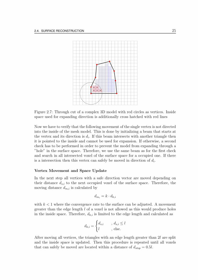
Figure 2.7: Through cut of a complex 3D model with red circles as vertices. Insidespace used for expanding direction is additionally cross hatched with red lines

Now we have to verify that the following movement of the single vertex is not directedinto the inside of the mesh model. This is done by initializing a beam that starts atthe vertex and its direction is di. If this beam intersects with another triangle thenit is pointed to the inside and cannot be used for expansion. If otherwise, a secondcheck has to be performed in order to prevent the model from expanding through a”hole” in the surface space. Therefore, we use the same beam as for the first checkand search in all intersected voxel of the surface space for a occupied one. If thereis a intersection then this vertex can safely be moved in direction of di.

Vertex Movement and Space Update

In the next step all vertices with a safe direction vector are moved depending ontheir distance ds,i to the next occupied voxel of the surface space. Therefore, themoving distance dm,i is calculated by

dmi= k · dk,i

with k < 1 where the convergence rate to the surface can be adjusted. A movementgreater than the edge length l of a voxel is not allowed as this would produce holesin the inside space. Therefore, dk,i is limited to the edge length and calculated as

dk,i =

{

ds,i , ds,i ≤ l

l , else.

After moving all vertices, the triangles with an edge length greater than 2l are splitand the inside space is updated. Then this procedure is repeated until all voxelsthat can safely be moved are located within a distance of dstop = 0.5l.


Fig. 2.8 portrays the update vectors with a length of dstop for each vertex of ourexample with a black arrow. If an update vector does not reach the surface space,represented by the red filled rectangles, the corresponding vertex can safely be movedand is coloured in green. In this case we set one of the occupied voxels of the surfacespace to be free in order to illustrate a hole in this space. All vertices that can notbe moved, either because they are to close to the surface or because there is a holein direction of the update vector, are coloured in red.

Figure 2.8: Through cut of a complex 3D model with circles as vertices. Verticesthat can safely are green, else red.

2.4.2 Detailing

In the detailing stage the raw model is refined in order to recover details. Therefore,we utilize an iterative procedure that searches for nearby depth points and movethe vertices of the 3D model towards them. This is done with an adaptive findingrange lf in order to smoothly refine the model. It starts with a range of 2l where lis again the edge length of a voxel in inflating stage. It is then iteratively reducedto the minimum edge length lm of the model and is calculated as:

lf = lm + ((imax − icur)/imax · (l − lm))

where imax is the maximum iteration number and icur the current iteration num-ber. Furthermore, lf is used to adapt the edge length of the triangles. Therefore,after each iteration all edges are checked and their corresponding triangles are splitaccording to the method of Lachaud and Montanvert [34] if their length is greaterthan lf .


2.4.3 Smoothing and Regularizing

Inflating a mesh model leads to irregular triangles and rough surfaces. A key pointto a good mesh model is therefore smoothing and regularizing technologies. In thefollowing subsection we explain two methods that can be applied in order to coverthose.

Smoothing

In order to smooth sharp edges that occur due to the surface reconstruction algo-rithm, local surface smoothing needs to be applied on the build mesh. We concen-trate on a method which uses the implemented triangle topology with its informationabout the local triangle neighbourhood. For that first normals for each vertex haveto be estimated. The normal nt,i for triangle ti can be produced by calculating thecross product denoted by (·)× (·) of two of its edges e1 and e2 by using

nt,i =e1|e1|

×e2|e2|

.

Attention has to be paid to the correct order for e1 and e2 to produce a normalthat points outside the mesh model. By averaging the normals of all m triangles acertain vertex vi is part of we can estimate the normal nv,i for this vertex

nv,i =

∑m

i=1 nt,i∑m

i=1 |nt,i|.

For the next step we need to estimate the local change of the surface. Therefore, wecollect for the triangle ti from the three neighbouring triangles those vertices thatare not shared with ti and denote this set as Ni. For each vertex vj in Ni we cannow calculate the distace dj,i between vertex vj and a virtual surface represented bythe normal nv,i with

dj,i = nv,i ◦ (vj − vi).

In fig. 2.9 this issue is illustrated. The blue dashed line represent the virtual surfaceof vi and the distance dj,i is drawn as doubled arrow. Please note, that the surfaceof the normal nv,i does not correspond to the surface represented by the triangleti. This is due to the fact that each vertex is part of more than one triangle andtherefore using only one triangle’s surface would not fully represent the local surface.

vi

vj

nv,i

dj,i

Figure 2.9: Illustration of vertex vj and its counter vertex vc,j


The angle αi,j between the surfaces of triangle ti and its neighbour tj can be calcu-lated with

αi,j = arccos

(

nv,i ◦ nv,j

|nv,i||nv,j |

)

.

As next step we map each vertex of Ni to its counter vertex vc,j of the triangle ti.Meaning, we form a vertex pair with vj and that vertex of ti that is not commonin both triangles. An illustration can be found in fig. 2.10. Here, the red and bluefilled circles represent vj and vc,j, respectively.

vc,j vjti tj

Figure 2.10: Illustration of vertex vj and its counter vertex vc,j

By making use of dj,i and αi,j we can now smoothen the surface in a local area.Therefore, we move vj towards the virtual surface and vice versa, the surface towardsvj, meaning that vi is moved in the opposite direction. For that the update value uis calculated as

u = ksdj,i sin((conf(vi)− conf(vj))π + 1)

where conf(·) represents the estimation confidence of a vertex and ks is a factorto regulate the movement that has to be smaller than 0.5. In order to limit thesmoothing to a certain angle range, we can adapt u with a minimum αmin andmaximum angle αmax

u =

0 , αi,j − αmin < 0

0 , αmax − αi,j < 0

u , else.

The update rule for vi,k and vj,k where the subscript k denotes the time step is then

vi,k = vi,k−1 + unv,i

vj,k = vj,k−1 − unv,i.


vc,j

vj

nv,i

u · nv,i

−u · nv,i

Figure 2.11: Update procedure applied on vertex vj and its counter vertex vc,j

Fig. 2.11 illustrates the update procedure. Here the two vertices vc,j and vj aremoved in direction of the normal of vi with −u and u as moving distance.

Regularizing

As only vertices are moved, spiky mesh artefacts are possible to occur. These arte-facts can lead to irregularities in the mesh during the progression of the process.In order to prevent this a simple procedure helps to regularize a mesh without toomuch of an influence onto the model structure. An example for irregularities can befound in fig. 2.12. Here some of the triangles are long and spiky. Just by movingthe vertex into the middle of the mesh, the triangles are more evenly distributed.The surface of this mesh is only slightly changed.

Figure 2.12: By moving the vertex in the middle the mesh can be regularized

In order to cope with such phenomenons, we need to analyse all edges of each vertexand their relation to each other. By calculating the angle between two edges ofone edge, we get a hint on how regular the triangles between those edges are. Forour purpose we want the three angles of all triangles to be near 60◦. For example,looking onto the two red edges in fig. 2.12 we can see that their angle αreg is farfrom being 60◦. The angle between two edges e1 and e2 can be calculated by

αreg = arccos

(

e1 ◦ e2|e1||e2|

)

.


As we want this angle to be nearly 60◦ we move the cosine of αreg to be almost 0 ifthe angle is close to 60◦ and denote the variable to be regulated as a:

a = cos(αreg)− 0.5

In order to construct an update vector uvec that is on the plane spanned through e1and e2 and points orthogonal to e2 away from e1 we use the cross product

uvec = e2 × (e2 × e1).

Fig. 2.13 illustrates the construction of uvec.

uvec

Figure 2.13: Constructed update vector uvec

The update movement un for the not shared vertex of e2 is then calculated with aregulating factor kreg by

un = kreg · a · uvec

and for the shared we use the negative direction

us = −un.

By applying this procedure on all edges of a vertex, we can regularize the trianglesof a mesh with only low impact on the surface.

31

Chapter 3

Experimental Results

In this chapter, we present results of two experiments made using real robotic sys-tem. The first experiment was performed with a KUKA omniRob platform. Theinterested reader is referred to [38] for more information regarding the omniRobplatform. This robot is extended with a Pan Tilt Unit (PTU) on which a stereosystem is mounted as illustrated in fig. 3.2. Please note that in this figure an AsusXtion is on top of the stereo system which is not used. The stereo system consistsof two Guppy Pro F-125 cameras from Allied Vision Technologies with a resolutionof 1292x964 pixels, for more information refer to [39]. For gripping and holding ob-jects, a KUKA LWR 4+ manipulator [40] is extended with a Schunk PG 70 Gripper.The whole setup is illustrated in fig. 3.1.

Figure 3.1: Experimental setup with KUKA omniRob and stereo system

32 CHAPTER 3. EXPERIMENTAL RESULTS

Figure 3.2: Stereo system mounted on a PTU

For comparison reasons, we performed a second experiment using preciser hardware.The experimental setup consisted of a KUKA KR16-2 manipulator, see [41], with aScanControl 2700 − 100 laser striper from Micro-Epsilon [42] mounted on it. Bothdevices are significantly more accurate in comparison to the KUKA LWR4+ and theused stereo-system. See fig. 3.3 for an illustration. For evaluating our approach weuse two objects that vary in shape and texture. One to which we will refer as filterobject in the following is portrayed in fig. 3.4, the other is a coffee package shown infig. 3.5. Both objects shown in the images are exemplarily gripped with a Schunk PG70 Gripper. Please note, that these are not the exact poses of the objects that can beseen in the following sections. All scans are compared to manually scanned meshes.These were made with a hand held high precision scanner and manually aligned.Those 3D models are shown in fig. 3.6 and fig. 3.7. In the following, we look at thedifferent stages of our approach individually. Here we used the first experimentalsetup. First we will show the generation and evaluation of viewpoints which isfollowed by the results of the ICP registration. After the filtering phase, we examinethe surface reconstruction step which is divided into the inflating and the detailingstage. Next, we compare the build models to the hand made meshes. Finally, wewill examine the resulting mesh models gained with the second experimental setupand compare those models with the hand made meshes as well.

33

Figure 3.3: Experimental setup with KUKA KR16 and ScanControl laser striper

Figure 3.4: The filter object gripped with a PG 70 Gripper


Figure 3.5: The coffee package gripped with a PG 70 Gripper

Figure 3.6: High precision scan of the filter object

35

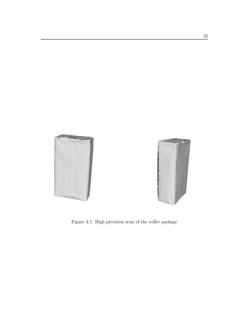
Figure 3.7: High precision scan of the coffee package


3.1 Viewplanning

The first scan for measuring a new object is a predefined viewpoint that capturespart of the gripper and most certainly one side of the object. Based on the firstscan, the NBV voxelspace is updated. An example for this with the filter object canbe seen in fig. 3.8. Here, the state of the voxels are coloured as: White for occupiedvoxel, grey for unknown (as initial state) and black for border voxel. Light yellowvoxels represent the inside space.Please note that as we know where the gripper is, its corresponding space is set tooccupied and does not influence as well as is not influenced by the NBV planningprocess. Furthermore, the space around the gripper is set to unknown and is as wellnot influenced and does not influence this process. These two assumptions are madeas the object is located above the gripper and therefore, both areas are only shownfor illustration reasons.

Figure 3.8: Voxelspace for determining the next best view. White voxels are occu-pied, grey unknown, black border voxel and yellow are inside voxel

For the following figures we will print this space for illustration reasons. The gen-erated viewpoints can be seen in fig. 3.9. Here, the biggest part of viewpoints islocated on places where both, occupied voxels and inside space most certainly canbe scanned.After filtering the viewpoints locally, the next best viewpoint is chosen. An illustra-tion for this is given in fig. 3.10. Here, the NBV is shown as the only green dot. Allother viewpoints are coloured in red.After performing a series of scans, the final NBV space has no border voxel and noviewable inside space. In fig. 3.11 an example for the filter object is shown. Heresome occupied voxels obviously can be classified as outliers. An advantage of thepresented method is that those outliers do not affect the NBV planning process, asthere is no inside space near to them.

3.1. VIEWPLANNING 37

Figure 3.9: All generated viewpoints together with the NBV space

In the presented example, 33 scans where made until no viewpoints could be gen-erated. This means, that all viewable voxels are on the one hand occupied and onthe other have at least a certain amount of measurements assigned to them. In thegiven example, we set the minimum of scan points per voxel to 5.


Figure 3.10: Filtered and evaluated viewpoints together with the NBV space. Thegreen dot represents the next best viewpoint

Figure 3.11: The final NBV space

3.2. REGISTRATION 39

3.2 Registration

After performing a series of scans, we can now start the preprocess stage of ouralgorithm.

Figure 3.12: Two unaligned scans of the filter object

Fig. 3.12 and fig. 3.13 show the data of two scans - illustrated as red points for onescan and green points for the second scan - of the filter and the coffee package afterapplying a box filter to remove all not needed points. Obviously, those scans needto be aligned for further proceedingsAfter registration using the ICP algorithm a significant improvement could beachieved which can be seen in fig. 3.14 and fig. 3.15, where the white points representthe template scan. The not aligned scan is illustrated as red points and the scanafter registration as green points.Although, the alignment of both scans can be improved through ICP, an errorthrough measuring failures can still be recognised that is too high for surface re-construction. Fig. 3.16 illustrates this. Here, in the template image (white points)a measuring failure occurred that is highlighted with a blue ellipse. Unfortunately,this result yields for many scans taken with the given hardware. Therefore, we willtake a closer look on the results of our filtering stage in the next section.


Figure 3.13: Two unaligned scans of the coffee package

Figure 3.14: Two scans of the filter object, white points represent the templateimage, red points the unaligned scan and green points the aligned scan

3.2. REGISTRATION 41

Figure 3.15: Two scans of the coffee package, white points represent the templateimage, red points the unaligned scan and green points the aligned scan

Figure 3.16: Two scans of the filter object, white points represent the templateimage, red points the unaligned scan and green points the aligned scan. The blueellipse shows the remaining error through measuring failure


3.3 Filtering

As the filtering stage is applied globally on all images, fig. 3.17 and fig. 3.18 showthe combined and registered scans in one image for the coffee package and the filterobject.

Figure 3.17: All scans of the filter object combined

After filtering those, the result is illustrated in fig. 3.19 and fig. 3.20. In both cases,the number of measurements is significantly reduced. Most of the multiple measuredsurfaces that are displaced are now combined to a more continuous surface. Oneside effect of the filtering stage is that most outliers are vanished as they have notenough neighbouring points to support the hypothesis of them being at a certainpoint in space.

By changing the noise radius we can trade between measurement confidence anddetails. The larger this parameter is, the less edges are detected, see fig. 3. Here,we highlight an edge of the real object with a blue ellipse. Obviously, this edge iscompared to the original parameters blurred out.

By changing the reduction radius, the point density can be changed and outliersfiltered. If this radius is too small, only the noise radius is used for determining themeasurement confidence, as no direct neighbours can be found. This can lead - incase of a poorly chosen parameter - to large measurement holes, if too many pointsare filtered. Fig. 3.22 illustrates this example.

3.3. FILTERING 43

Figure 3.18: All scans of the coffee package combined

On the other hand, if the reduction radius is too large, the filter would produce atoo great distance between the remaining measurements, refer to fig. 3.23. This willlead to holes in the surface space for the inflating stage and can be seen in fig. 3.24.Another side effect of this is that again, small details would be lost by averaging themeasurements.


Figure 3.19: All scans of the filter object combined after filtering

Figure 3.20: All scans of the coffee package combined after filtering

3.3. FILTERING 45

Figure 3.21: The original filter with double noise radius, blue ellipse illustrate theblurring of an edge

Figure 3.22: The original filter with a too small reduction radius leads to holes inthe scan data


Figure 3.23: The original filter with double reduction radius

Figure 3.24: The resulting surface space for the inflating stage produced by doublereduction radius


3.4 Surface Reconstruction

After registrating and filtering the scanned data, the inflating stage is performed onboth objects. The results can be seen in fig. 3.25 and fig. 3.26. The mesh illustratesthe surface of the real objects roughly and can be further processed.

Figure 3.25: The mesh of the filter object after the inflating stage

For preparing the mesh for the detailing stage, we use the smoothing and regularizingtechniques and get a better formed model that can be seen in fig. 3.27 and fig. 3.28.The surfaces are now a lot smoother and we have gained more regular triangles.The detailing stages tries to reconstruct more details from the scanned data. Itresults in meshes as fig. 3.29 and 3.30.Given the impreciseness and noisiness of both pose and depth measurement, thesurface reconstruction algorithm is able to build a raw mesh model of the presentedobjects. These models have the advantage of being watertight and therefore, repre-senting the surface of a real object in a more practical way.In fig. 3.31 and fig. 3.32 both, the manually made models and the automatic mod-els using the omniRob system are each shown in a single image. The automaticallyobjects can only give a rough estimation of the actual surface. The alignment of themodels was performed using the aforementioned ICP algorithm. The CoordinateRoot Mean Squared Error (cRMS) is the average point-to-point distance of pointsto their correspondences after alignment and is shown for both objects in tab. 3.4.

Object Correspondences cRMS [mm]Filter 24108 2.7963Coffee 18312 2.4753


Figure 3.26: The mesh of the coffee package after the inflating stage

Please note that in case of the models created using the omniRob platform, partof the grab jaws are modelled as well, refer to the left picture of fig. 3.31 andfig. 3.32. Therefore, for not falsifying the result, we cut off those parts of themodel. Visible in the right picture of fig. 3.31 and fig. 3.32, for both objects somesurfaces are clearly displaced. Furthermore, please note that for the coffee package,the automatically scanned mesh is thicker than the original object and thereforedisplaced after alignment. For those reasons, the registration results in an cRMS of∼ 2.8mm for the filter object and ∼ 2.5mm for the coffee package.As utilizing hardware that produce highly noisy measurements prevents us fromestimating the accuracy of our approach, the next section analyses this aspect usinga different hardware setup.


Figure 3.27: The mesh of the filter object before the detailing stage

Figure 3.28: The mesh of the coffee package before the detailing stage


Figure 3.29: The final mesh of the filter object

Figure 3.30: The final mesh of the coffee package


Figure 3.31: Comparison of the manually (white) and automatically (red) mademodels for the filter object

Figure 3.32: Comparison of the manually (white) and automatically (red) mademodels for the coffee package


3.5 Laser Scanned Objects

For comparison we used a different experimental setup consisting of a KUKA KR16-2 manipulator, see [41], with a ScanControl 2700 − 100 laser striper from Micro-Epsilon [42] mounted on it. Both devices are significantly more accurate in compar-ison to the KUKA LWR4+ and the used stereo-system. Using our surface recon-struction algorithm combined with the new hardware on the filter object and thecoffee package, the created mesh models show a highly improved result as can beseen in fig. 3.33 and fig. 3.34.

Figure 3.33: The final mesh of the filter object using a laser striper

3.5. LASER SCANNED OBJECTS 53

Figure 3.34: The final mesh of the coffee package using a laser striper

Please note, that for the filter object the top cylinder is missing. This is due to thesmall connection between the body and this cylinder. Another reason is that thereare only few noisy measurements of this connection and consequently, the meshcannot inflate through this area.For both objects, we mapped the estimated variance of the distance from vertex tonearby measurements as colour to the triangles. Here, red illustrates a large varianceor even no measurements at all while green represents a small variance. This canbe interpreted as confidence of the position of the triangles and their vertices.In fig. 3.35 and fig. 3.36, the manually scanned and the automatically build modelare illustrated together. The alignment for both was computationally done with theaforementioned ICP algorithm. Its result gives a hint on the preciseness of the modeland can be seen in table 3.5. Here, the cRMS is for the coffee package under 0.7mm.For the filter object, a larger error occurs as on the one hand the top cylinder is notmodelled and on the other hand, a number of high variance parts show that somedetails of the object were not scanned.

Object Correspondences cRMS [mm]Filter 26397 1.5590Coffee 22491 0.6875

Nevertheless, for both objects we can state that our surface reconstruction approachis able to recover most details and realistically reconstruct the scanned object.


Figure 3.35: Comparison of the manually (white) and automatically (red) mademodels for the filter object

Figure 3.36: Comparison of the manually (white) and automatically (red) mademodels for the coffee package

55

Chapter 4

Conclusion and Outlook

In this work, we implemented a method for surface reconstruction. For acquiringthe sensor data, different poses have to be planned. Therefore, we implemented aNBV planning algorithm, that allows for automatic data acquisition. This is donevia estimating the space inside the to be scanned object. From this space, a pointis projected through the surface or possible borders with a user defined distance,to obtain the position of a viewpoint candidate. The information gain for thoseviewpoint candidates is then estimated and the highest information gain is chosenas next viewpoint.Once the data is gained, we have to cope with pose errors. Therefore, we use theiterative closest point (ICP) algorithm. While in most cases, the ICP algorithm reli-ably recovers the pose of the measurement, some cases remain that compromise thesurface reconstruction. We developed a filtering stage in order to filter those andoutliers for improving the measurement confidence. By comparing the estimatednormals of nearby points and combining similar measurements, an estimation forthe real surface can be calculated.Through inflating, we can build a raw mesh model of the scanned object. For this,a further space needs to be created that represents the inside space of the mesh.By projecting from this space through the single vertices, the expanding directioncan be determined. For avoiding growing through holes in the measurements, wefirst cluster the measurements in a voxelspace. A safe movement of each vertex canbe determined by searching in expanding direction for a voxel with measurementsattached to it. Through this, vertices that grow through holes in the surface spacecan be avoided.By applying smoothing and regularizing techniques that highly depend on the con-nected topology of a watertight mesh, we prepare the model for the detailing stagein order to gain regular triangles with a smooth surface. In this stage, we try torecover finer details of the model by moving vertices to nearby measurement points.We show experimentally that facing imprecise and noisy data, a coarse model canbe recovered. Even though this model is watertight, but faces high noise using thesetup of omniRob platform. By using preciser hardware, a surface model with fine

56 CHAPTER 4. CONCLUSION AND OUTLOOK

details can be build. All mesh models are watertight, meaning there are no holes inthe mesh. This is achieved through a deformable mesh with topology adaptation.Those meshes can be used for object recognition or planning of manipulation task.Based on this, pick and place tasks can be implemented as gripping and placingof an object can be planed using the mesh model. Consequently, having a meshrepresentation of an object, is one step towards enabling robots to assist humans.Through calculating the distance variance from vertex to measurements, poorlyscanned areas of the model can be detected. Consequently, in future work a postmodelling scan process can improve details of a mesh model by measuring those ar-eas. As the mesh is deformable, those new scans can directly push the correspondingtriangles to the actual surface.Another improvement of our approach might to cluster the scanned data and per-form a surface reconstruction on the acquired clusters. For our filter object thiswould mean to separate the scanned data for the body and the top cylinder. Forboth clusters a mesh model needs to be build. Based on this, merging techniquesneed to be developed in order to combine several meshed parts of an object withoutloosing the topology of the mesh.Further development of this approach might include performance optimization. There-fore, parallel processing is one important key feature. One approach to achieve thatis to parallelize the stages of our approach. As only a voxel based surface represen-tation with as few as possible holes is necessary for the inflating stage, the scanningphase of the algorithm can be divided into an exploring stage and a fine measuringphase. For the first phase, only a small amount of measurements would be necessaryto cover all surfaces of an object. This step can be achieved by manipulating theevaluation parameters of our NBV approach. Furthermore, lowering the minimumnumber of measurements per voxel to 1, the needed space could be generated quicker.After reaching a certain surface coverage, the inflating stage could be started in par-allel to the fine measuring phase. In the latter, the NBV algorithm is adjusted tothe original parameters, for increasing measurement confidence.After the inflating stage finishes, the detailing stage can be initiated and the newgained scans can be directly forwarded to it. This could result in a large perfor-mance improvement.A second attempt for performance optimisation is to parallelize the single steps ofthe algorithms. To a large extent, many calculations are performed individually foreach point or vertex. Making use of the concept of General Purpose Computationon Graphics Processing Unit (GPGPU) can largely reduce processing time by par-allelizing those calculations.A further improvement could consist of a surface reconstruction that performs di-rectly after the first scan. This can be achieved through adapting the inflatingstage to perform on a not closed voxel surface representation. Therefore, we need toenable safe movements to influence the movements of neighbouring and connectedvertices. Consequently, a smoother inflating of a mesh can be obtained and the im-pact of large holes can be significantly reduced. Based on this, a parallel scanning

57

and meshing approach can be implemented.

58 CHAPTER 4. CONCLUSION AND OUTLOOK

LIST OF FIGURES 59

List of Figures

1.1 Inversion of the shared edge to create better posed triangles . . . . . 13

1.2 Merging two vertices whose distance is below a threshold . . . . . . . 14

1.3 Splitting a triangle into four smaller triangles . . . . . . . . . . . . . 14

1.4 Splitting a triangle and propagating it onto the following. The dashedlines represent the propagated cuts. . . . . . . . . . . . . . . . . . . . 15

1.5 Splitting a triangle into two smaller triangles . . . . . . . . . . . . . . 15

2.1 Overview of the scanning and surface reconstruction algorithm . . . . 18

2.2 Example for a voxelpace representation using octrees . . . . . . . . . 18

2.3 Overview of the surface reconstruction algorithm . . . . . . . . . . . . 22

2.4 Through cut of the seed model in a voxelspace . . . . . . . . . . . . . 23

2.5 Through cut of a complex 3D model . . . . . . . . . . . . . . . . . . 24

2.6 Through cut of a complex 3D model with surface space as red filledand inside space as blue cross hatched rectangles . . . . . . . . . . . 24

2.7 Through cut of a complex 3D model with red circles as vertices. Insidespace used for expanding direction is additionally cross hatched withred lines . . . . . . . . . . . . . . . . . . . . . . . . . . . . . . . . . . 25

2.8 Through cut of a complex 3D model with circles as vertices. Verticesthat can safely are green, else red. . . . . . . . . . . . . . . . . . . . . 26

2.9 Illustration of vertex vj and its counter vertex vc,j . . . . . . . . . . . 27

2.10 Illustration of vertex vj and its counter vertex vc,j . . . . . . . . . . . 28

2.11 Update procedure applied on vertex vj and its counter vertex vc,j . . 29

2.12 By moving the vertex in the middle the mesh can be regularized . . . 29

2.13 Constructed update vector uvec . . . . . . . . . . . . . . . . . . . . . 30

3.1 Experimental setup with KUKA omniRob and stereo system . . . . . 31

3.2 Stereo system mounted on a PTU . . . . . . . . . . . . . . . . . . . . 32

3.3 Experimental setup with KUKA KR16 and ScanControl laser striper 33

3.4 The filter object gripped with a PG 70 Gripper . . . . . . . . . . . . 33

3.5 The coffee package gripped with a PG 70 Gripper . . . . . . . . . . . 34

3.6 High precision scan of the filter object . . . . . . . . . . . . . . . . . 34

3.7 High precision scan of the coffee package . . . . . . . . . . . . . . . . 35

60 LIST OF FIGURES

3.8 Voxelspace for determining the next best view. White voxels areoccupied, grey unknown, black border voxel and yellow are inside voxel 36

3.9 All generated viewpoints together with the NBV space . . . . . . . . 373.10 Filtered and evaluated viewpoints together with the NBV space. The

green dot represents the next best viewpoint . . . . . . . . . . . . . . 383.11 The final NBV space . . . . . . . . . . . . . . . . . . . . . . . . . . . 383.12 Two unaligned scans of the filter object . . . . . . . . . . . . . . . . . 393.13 Two unaligned scans of the coffee package . . . . . . . . . . . . . . . 403.14 Two scans of the filter object, white points represent the template

image, red points the unaligned scan and green points the aligned scan 403.15 Two scans of the coffee package, white points represent the template

image, red points the unaligned scan and green points the aligned scan 413.16 Two scans of the filter object, white points represent the template

image, red points the unaligned scan and green points the alignedscan. The blue ellipse shows the remaining error through measuringfailure . . . . . . . . . . . . . . . . . . . . . . . . . . . . . . . . . . . 41

3.17 All scans of the filter object combined . . . . . . . . . . . . . . . . . . 423.18 All scans of the coffee package combined . . . . . . . . . . . . . . . . 433.19 All scans of the filter object combined after filtering . . . . . . . . . . 443.20 All scans of the coffee package combined after filtering . . . . . . . . 443.21 The original filter with double noise radius, blue ellipse illustrate the

blurring of an edge . . . . . . . . . . . . . . . . . . . . . . . . . . . . 453.22 The original filter with a too small reduction radius leads to holes in

the scan data . . . . . . . . . . . . . . . . . . . . . . . . . . . . . . . 453.23 The original filter with double reduction radius . . . . . . . . . . . . 463.24 The resulting surface space for the inflating stage produced by double

reduction radius . . . . . . . . . . . . . . . . . . . . . . . . . . . . . . 463.25 The mesh of the filter object after the inflating stage . . . . . . . . . 473.26 The mesh of the coffee package after the inflating stage . . . . . . . . 483.27 The mesh of the filter object before the detailing stage . . . . . . . . 493.28 The mesh of the coffee package before the detailing stage . . . . . . . 493.29 The final mesh of the filter object . . . . . . . . . . . . . . . . . . . . 503.30 The final mesh of the coffee package . . . . . . . . . . . . . . . . . . . 503.31 Comparison of the manually (white) and automatically (red) made

models for the filter object . . . . . . . . . . . . . . . . . . . . . . . . 513.32 Comparison of the manually (white) and automatically (red) made

models for the coffee package . . . . . . . . . . . . . . . . . . . . . . . 513.33 The final mesh of the filter object using a laser striper . . . . . . . . . 523.34 The final mesh of the coffee package using a laser striper . . . . . . . 533.35 Comparison of the manually (white) and automatically (red) made

models for the filter object . . . . . . . . . . . . . . . . . . . . . . . . 543.36 Comparison of the manually (white) and automatically (red) made

models for the coffee package . . . . . . . . . . . . . . . . . . . . . . . 54

LIST OF FIGURES 61

List of Abbreviations

NBV Next Best View. . . . . . . . . . . . . . . . . . . . . . . . . . . . . . . . . . . . . . . . . . . . . . . . . . . . . . . .6

cRMS Coordinate Root Mean Squared Error . . . . . . . . . . . . . . . . . . . . . . . . . . . . . . . . 47

ICP Iterative Closest Point . . . . . . . . . . . . . . . . . . . . . . . . . . . . . . . . . . . . . . . . . . . . . . . . . 6

MVS Mass Vector Sum . . . . . . . . . . . . . . . . . . . . . . . . . . . . . . . . . . . . . . . . . . . . . . . . . . . . . . 6

PTU Pan Tilt Unit. . . . . . . . . . . . . . . . . . . . . . . . . . . . . . . . . . . . . . . . . . . . . . . . . . . . . . . . .31

GPGPU General Purpose Computation on Graphics Processing Unit. . . . . . . . . . .56

62 LIST OF FIGURES

BIBLIOGRAPHY 63

Bibliography

[1] D. Lamb, D. Baird, and M. A. Greenspan, “An automation system for industrial3-d laser digitizing,” in 1999. Proceedings. Second International Conference on3-D Digital Imaging and Modeling, 1999.

[2] S. Khalfaoui, R. Seulin, Y. Fougerolle, and D. Fofi, “View planning approachfor automatic 3d digitization of unknown objects,” in Computer Vision ECCV2012. Workshops and Demonstrations. Springer Berlin Heidelberg, 2012.

[3] B. Loriot, R. Seulin, and P. Gorria, “Non-model based method for an automa-tion of 3d acquisition and post-processing,” Electronics Letters on ComputerVision and Analysis, 2008.

[4] N. A. Massios and R. B. Fisher, “A best next view selection algorithm incor-porating a quality criterion,” in BMVC, 1998.

[5] S. Kriegel, T. Bodenmuller, M. Suppa, and G. Hirzinger, “A surface-based next-best-view approach for automated 3d model completion of unknown objects,”in IEEE International Conference on Robotics and Automation (ICRA), 2011.

[6] S. Kriegel, C. Rink, T. Bodenmuller, A. Narr, M. Suppa, and G. Hirzinger,“Next-best-scan planning for autonomous 3d modeling,” in IEEE/RSJ Inter-national Conference on Intelligent Robots and Systems IROS, 2012.

[7] S. Kriegel, C. Rink, T. Bodenmuller, and M. Suppa, “Efficient next-best-scanplanning for autonomous 3d surface reconstruction of unknown objects,” Jour-nal of Real-Time Image Processing, pp. 1–21, 2013.

[8] Y. Chen and G. Medioni, “Object modelling by registration of multiple rangeimages,” Image and vision computing, vol. 10, no. 3, pp. 145–155, 1992.

[9] P. J. Besl and N. D. McKay, “A method for registration of 3-d shapes,” IEEETransactions on Pattern Analysis and Machine Intelligence, vol. 14, no. 2, pp.239–256, Februrary 1992.

[10] S. Rusinkiewicz and M. Levoy, “Efficient variants of the icp algorithm,” in ThirdInternational Conference on 3D Digital Imaging and Modeling (3DIM), 2001.

64 BIBLIOGRAPHY

[11] R. Toldo, A. Beinat, and F. Crosilla, “Global registration of multiple pointclouds embedding the generalized procrustes analysis into an icp framework,”in 3DPVT 2010 Conference, 2010.

[12] T. Masuda, K. Sakaue, and N. Yokoya, “Registration and integration of multiplerange images for 3-d model construction,” in Proceedings of the 13th Interna-tional Conference on Pattern Recognition, 1996.

[13] Z. Zhang, “Iterative point matching for registration of free-form curves andsurfaces,” International Journal for Computer Vision, vol. 13, pp. 119–152,1994.

[14] P. J. Neugebauer, “Geometrical cloning of 3d objects via simultaneous regis-tration of multiple range images,” in 1997 International Conference on ShapeModeling and Applications, 1997.

[15] D. Chetverikov, D. Svirko, D. Stepanov, and P. Drsek, “The trimmed iterativeclosest point algorithm,” in International Conference on Pattern Recognition,2002, pp. 545–548.

[16] D. A. Simon, “Fast and accurate shape-based registration,” Ph.D. dissertation,Carnegie Mellon University, 1996.

[17] J. Zhu, N. Zheng, Z. Yuan, and S. Du, “Point-to-line metric based iterativeclosest point with bounded scale,” in ICIEA 2009. 4th IEEE Conference onIndustrial Electronics and Applications, 2009.

[18] M. Potmesil, “Generating models of solid objects by matching 3d surface seg-ments,” in IJCAI, 1983.

[19] M. Suppa, “Autonomous robot work cell exploration using multisensory eye-in-hand systems,” Ph.D. dissertation, Gottfried Wilhelm Leibniz Universit”atHannover, 2008.

[20] C. V. Nguyen, S. Izadi, and D. Lovell, “Modeling kinect sensor noise for im-proved 3d reconstruction and tracking,” in 2012 Second International Con-ference on3D Imaging, Modeling, Processing, Visualization and Transmission(3DIMPVT), 2012.

[21] F. Pomerleau, A. Breitenmoser, M. Liu, F. Colas, and R. Siegwart, “Noise char-acterization of depth sensors for surface inspections,” in 2012 2nd InternationalConference on Applied Robotics for the Power Industry (CARPI), 2012.

[22] A. Segal, D. Haehnel, and S. Thrun, “Generalized-icp,” in Robotics: Scienceand Systems, 2009.

BIBLIOGRAPHY 65

[23] G. Turk and M. Levoy, “Zippered polygon meshes from range images,” in Pro-ceedings of the 21st Annual Conference on Computer Graphics and InteractiveTechniques, 1994.

[24] G. Pandey, J. McBride, S. Savarese, and R. M. Eustice, “Visually bootstrappedgeneralized icp,” in 2011 IEEE International Conference on Robotics and Au-tomation (ICRA), 2011.

[25] K. Pulli, “Multiview registration for large data sets,” in 1999. Proceedings.Second International Conference on 3-D Digital Imaging and Modeling, 1999.

[26] S. Krishnan, P. Y. Lee, J. B. Moore, and S. Venkatasubramanian, “Globalregistration of multiple 3d point sets via optimization-on-a-manifold,” in Euro-graphics Symposium on Geometry Processing, 2005, pp. 187–196.

[27] N. J. Mitra, N. Gelfand, H. Pottmann, and L. Guibas, “Registration ofpoint cloud data from a geometric optimization perspective,” in Proceedingsof the 2004 Eurographics/ACM SIGGRAPH symposium on Geometry process-ing. ACM, 2004, pp. 22–31.

[28] M. Kass, A. Witkin, and D. Terzopoulos, “Snakes: Active contour models,”International journal of computer vision, vol. 1, no. 4, pp. 321–331, 1988.

[29] J. V. Miller, D. E. Breen, W. E. Lorensen, R. M. O’Bara, and M. J. Wozny,“Geometrically deformed models: a method for extracting closed geometricmodels form volume data,” in ACM SIGGRAPH Computer Graphics, vol. 25,no. 4. ACM, 1991, pp. 217–226.

[30] M. Vasilescu and D. Terzopoulos, “Adaptive meshes and shells: Irregular tri-angulation, discontinuities, and hierarchical subdivision,” in In Proceedings ofComputer Vision and Pattern Recognition conference, 1992.

[31] J.-O. Lachaud and A. Montanvert, “Deformable meshes with automated topol-ogy changes for coarse-to-fine three-dimensional surface extraction,” MedicalImage Analysis, vol. 3, no. 2, pp. 187 – 207, 1999.

[32] J.-Y. Park, T. McInerney, D. Terzopoulos, and M.-H. Kim, “A non-self-intersecting adaptive deformable surface for complex boundary extraction fromvolumetric images,” Computers & Graphics, vol. 25, no. 3, pp. 421–440, 2001.

[33] Y. Chen and G. Medioni, “Description of complex objects from multiple rangeimages using an inflating balloon model,” Computer Vision and Image Under-standing, vol. 61, no. 3, pp. 325–334, 1995.

[34] A. Lachaud, Jacques-Olivier; Montanvert, “Deformable meshes with automatedtopology changes for coarse-to-fine three-dimensional surface extraction,” Med-ical Image Analysis, 1999.

66 BIBLIOGRAPHY

[35] O. Monga and R. Deriche, “3d edge detection using recursive filtering: appli-cation to scanner images,” in Computer Vision and Pattern Recognition, 1989.Proceedings CVPR ’89., IEEE Computer Society Conference on, Jun 1989, pp.28–35.

[36] A. Hornung, K. M. Wurm, M. Bennewitz, C. Stachniss, and W. Burgard, “Oc-toMap: An efficient probabilistic 3D mapping framework based on octrees,”Autonomous Robots, 2013.

[37] D. Jung and K. K. Gupta, “Octree-based hierarchical distance maps for col-lision detection,” in 1996 IEEE International Conference onRobotics and Au-tomation, 1996. Proceedings., 1996.

[38] (2014, November). [Online]. Available: http://www.kuka-labs.com/de/servicerobotics/mobile robotics/omniRob/

[39] (2014, November). [Online]. Available: http://www.alliedvisiontec.com/us/products/cameras/firewire/guppy-pro/f-125bc.html

[40] (2014, November). [Online]. Available: http://www.kuka-labs.com/en

[41] (2014, November). [Online]. Available: http://www.kuka-robotics.com/germany/en/products/industrial robots/low/kr16 2/start.htm

[42] (2014, November). [Online]. Available: http://www.micro-epsilon.de/laser-scanner/scanCONTROL/Laser-scanner-selection/index.html

http://www.kuka-labs.com/de/service_robotics/mobile_robotics/omniRob/

http://www.kuka-labs.com/de/service_robotics/mobile_robotics/omniRob/

http://www.alliedvisiontec.com/us/products/cameras/firewire/guppy-pro/f-125bc.html

http://www.alliedvisiontec.com/us/products/cameras/firewire/guppy-pro/f-125bc.html

http://www.kuka-labs.com/en

http://www.kuka-robotics.com/germany/en/products/industrial_robots/low/kr16_2/start.htm

http://www.kuka-robotics.com/germany/en/products/industrial_robots/low/kr16_2/start.htm

http://www.micro-epsilon.de/laser-scanner/scanCONTROL/Laser-scanner-selection/index.html

http://www.micro-epsilon.de/laser-scanner/scanCONTROL/Laser-scanner-selection/index.html

LICENSE 67

License

This work is licensed under the Creative Commons Attribution 3.0 Germany License.To view a copy of this license, visit http://creativecommons.org or send a letter toCreative Commons, 171 Second Street, Suite 300, San Francisco, California 94105,USA.

http://creativecommons.org/licenses/by/3.0/de/

Date post:	03-Jan-2022
Category:	Documents
Upload:	others
View:	3 times
Download:	0 times

Watertight Surface Reconstruction for Uncertain Data

Documents