Glasgow Theses Service http://theses.gla.ac.uk/ [email protected]Waterton, Richard James (2004) Analysis of the soliton solutions of a 3- level Maxwell-Bloch system with rotational symmetry. PhD thesis http://theses.gla.ac.uk/3867/ Copyright and moral rights for this thesis are retained by the author A copy can be downloaded for personal non-commercial research or study, without prior permission or charge This thesis cannot be reproduced or quoted extensively from without first obtaining permission in writing from the Author The content must not be changed in any way or sold commercially in any format or medium without the formal permission of the Author When referring to this work, full bibliographic details including the author, title, awarding institution and date of the thesis must be given
Waterton, Richard James (2004) Analysis of the soliton solutions of a 3-level Maxwell-Bloch system with rotational symmetry. PhD thesis http://theses.gla.ac.uk/3867/ Copyright and moral rights for this thesis are retained by the author A copy can be downloaded for personal non-commercial research or study, without prior permission or charge This thesis cannot be reproduced or quoted extensively from without first obtaining permission in writing from the Author The content must not be changed in any way or sold commercially in any format or medium without the formal permission of the Author When referring to this work, full bibliographic details including the author, title, awarding institution and date of the thesis must be given
Analysis of the Soliton Solutions of a 3-Level Maxwell-Bloch System with Rotational
Symmetry.
Richard James Waterton.
A thesis submitted in September 2004 to the Faculty of Engineering at the University of Glasgow for the degree of Ph. D.
(c) R. J. Waterton, 2004.
Abstract
The dynamics of soliton pulses for use in nonlinear optical devices is mathemat- ically modelled by Maxwell-Bloch systems of equations for the interaction of light with a uniform distribution of quantum-mechanical atoms. We study the Reduced Maxwell-Bloch (RMB) equations occuring when an ensemble of rota- tionally symmetric 3-level atoms is assumed. The model applies for on and off-
resonance conditions and is completely integrable using Inverse Scattering theory,
since it arises as the compatibility condition of a3x3 AKNS-system. Further-
more this integrability remains valid for all timescales of the optical field because
only the "one-way wave approximation" is required during the derivation. Solu-
tions are constructed in two ways: 1. Darboux-Bäcklund transforms are applied,
generating single soliton pulses of ultrashort (< 1ps) duration, and families of el- liptically polarised 2-solitons not possible in lower dimensional problems. 2. A
general Inverse Scattering scheme is developed and tested. The Direct Scattering
Problem is dealt with first to obtain a complete set of scattering data. Subse-
quently the Inverse Problem is solved both formally and then in explicit closed form for the special case that the reflection coefficients vanish for real values of the spectral parameter. In this case the main result is a determined system of n linear algebraic equations which yield the n-soliton solution of our RMB-system.
It is confirmed that the 1-solitons found by means of Darboux transforms are pre-
cisely the same as those given by the full mechanism of Inverse Scattering. Finally
we calculate the invariants of the motion for the RMB-equations, and derive an
evolution equation giving the variation with propagation distance of the invariant
functionals when the original RMB-system is modified by an arbitrary perturbing term. As an application dissipative effects on 1-solitons are considered.
3 Formulation and Integrability of the 3-Level Maxwell-Bloch Equa-
tions. 29
1
4 Use of Darboux-Bäcklund Transformations to find Fully Polarised Soliton Solutions. 37
4.1 Linearly Polarised 1-Soliton Solutions to the RMB-System..... 38
4.2 2-Soliton Solutions of the RMB-System ...... . .... . ... 43
5 Inverse Scattering for the RMB-System. 51
5.1 The Direct Scattering Problem ...... ........ ...... 53
5.1.1 Properties of the Transition Matrix . ............ 53
5.1.2 Integral Representations for the Transition Matrix. .... 57
5.1.3 Integral Representations for the Jost Solutions. ......
61
5.1.4 The Reduced Monodromy Matrix T(()........... 63
5.1.5 Integral Representations for the Transition Coefficients. . 66
5.1.6 Temporal Evolution of the Transition Coefficients. .... 68
5.1.7 The Scattering Matrix for the Direct Scattering Problem. . 70
5.1.8 Transition Coefficients for the Discrete Spectrum...... 73
5.1.9 Trace Formulae . ...................... 76
5.1.10 Statement of the Scattering Data ...... . ..... ... 80
5.2 The Inverse Scattering Problem . .................. 81
5.2.1 Derivation of the Riemann-Hilbert Problem for the RMB-
System . ........................... 81
5.2.2 Formal Solutions to the Inverse Problem. ......... 84
5.2.3 Soliton Solutions of the RMB-System............ 91
5.2.4 Existence and Uniqueness of Solutions to the Inverse Prob-
lem .............................. 93
2
6 Calculation of the Conserved Densities for the RMB-System. 98
7 Perturbative Effects in Real Optical Media. 110
7.1 Proof of the Evolution Equation for the Invariant Functionals.... 111
7.2 An Application of the Evolution Equation for the Invariant Func-
tionals ................................. 121
7.2.1 The Perturbed Model for an Absorbing Medium. ..... 121
7.2.2 First Order Dissipative Effects on 1-Solitons of the RMB- System............................ 124
8 Conclusions. 132
3
Chapter 1
Introduction.
1.1 Solitary Waves and Solitons.
As an essential preliminary we must first define the notion of a soliton. Referring to Ablowitz & Clarkson [1] p. 13, pp. 18-19 we make the definitions below:
A solitary wave solution of a nonlinear partial differential equation
N (x, t, u(x, t)) = 0,
where xER, tER are spatial and temporal variables and uER is the dependent
variable, is a travelling wave solution of the form
u (x, t) =f (x - ct) = f(4)
whose transition is from one constant asymptotic state as a -* -oo, to (possibly)
another constant asymptotic state as C -+ +oo.
A soliton is a localised solitary wave solution of a nonlinear equation (or system of
equations) which asymptotically preserves its shape and velocity upon nonlinear interaction with other solitary waves, or more generally with another (arbitrary)
4
localised disturbance.
Later (cf. p. 14) the more formal concept of an "n-soliton" will be introduced in the context of the Inverse Scattering Transform method (which is thoroughly described in Chapter 2).
1.2 Solitons in Nonlinear Optical Media.
A significant motivating factor for research into the solitary wave solutions of Maxwell-Bloch (MB) systems of differential equations was the original sugges- tion by Hasegawa and Tappert (1973) [2] that optical solitons could be used as bits in high capacity digital nonlinear communication systems. Basically Hasegawa
and Tappert's idea was that given sufficiently high optical power from a laser
source, short stable soliton pulses suitable for data transmission could be produced in a silica glass fibre, as a result of the balance arising between the effects of dis-
persion and the induced Kerr nonlinear interaction. Now the chief mathematical model representing this process is governed by the Nonlinear Schrödinger equa- tion. However, this equation is just one reduction of the Maxwell-Bloch system for the interaction of an electromagnetic plane wave with a uniform distribution
of quantum-mechanical atoms through dipole polarisation. In fact, if the atoms
are assumed simply to have two levels, a ground state and a single upper energy
state, then there are three cases:
1. The incident carrier wave is off-resonance with the atomic transition, and a Slowly Varying Envelope or Rotating Wave approximation is made.
2. The incident carrier wave is on-resonance, and an envelope approximation is made.
3. The incident carrier wave can have any frequency, and the atomic ensem- ble is supposed to have low density, allowing use of the "one-way wave approximation" (neglect of backscattered waves).
5
Cases 1 and 2 lead to the Nonlinear Schrödinger equation and the sine-Gordon equation respectively, which are famous nonlinear partial differential equations for complex wave envelopes. Both of these equations are integrable (i. e., analyt- ically solvable) by the Inverse Scattering Transform [3] [4] and have well doc-
umented soliton solutions. In particular, because of its relevance to fibre optic telecommunications, the Nonlinear Schrödinger equation has been exhaustively studied. We have included a brief discussion of soliton communication systems for background interest: see Section 1.4. Case 3 leads to the so-called 2-level Re- duced Maxwell-Bloch (RMB) equations which have importance modelling Self
Induced Transparency effects, where powerful ultrashort optical pulses are prop- agated without energy loss through a resonant dielectric medium. The Inverse Scattering scheme and solitons of this system were found by Bullough, Caudrey,
Eilbeck and Gibbon (1973) [5] [6] [7].
A substantially more complicated and less well researched problem is to integrate
the Maxwell-Bloch equations occuring when the constituent atoms of the ensem- ble have three distinct energy levels. We shall be investigating the soliton solutions of a recently discovered [8] exactly integrable 3-level Maxwell-Bloch system: the
system in question is essentially an extension of the 2-level RMB-equations to
allow circularly and elliptically polarised solutions, and is derived by assuming each of the individual atoms is rotationally symmetric with a zero level and two
separate orthogonal upper levels. As a general model it answers the need for an
analytically solvable basis with which to study near resonant interactions in non- insulating optical media, such as doped optical fibres, semi-conductors or vapours. Indeed its most pertinent application is probably in the description of pulse for-
mation within laser cavities. We note that whilst there exist other examples of integrable 3-level MB-systems [9] [10] [11], their formulation invariably neces- sitates envelope approximations. On the other hand, as will be seen in Chapter 3, the 3-level RMB-equations with rotational symmetry retain their integrability
right down to the carrier timescale, thus allowing physical interpretation of solu- tions at timescales as short as one optical cycle. Furthermore, in contrast to the
6
2-level model where by assumption there is no opportunity for the existence of orthogonal dipoles, soliton solutions of the 3-level equations may be circularly or
elliptically polarised.
1.3 Objectives and Layout.
The main purposes of this thesis may be summarised as follows:
. To devise a general integration scheme for the 3-level RMB-equations with rotational symmetry using the Inverse Scattering Transform method and ob- taining formulae for the n-soliton solution (N 3n> 1).
" To find a way of evaluating the effects of non-Hamiltonian perturbations on the soliton parameters.
These two problems are addressed in Chapters 5 and 7 respectively, after the req- uisite groundwork has been covered.
In Chapter 4 we employ Darboux-Bäcklund transforms to calculate expressions for the fully polarised 2-solitons of the RMB-system. Darboux transforms give a useful and relatively slick method of aquiring pure multi-soliton solutions of integrable nonlinear equations. Unfortunately though, this is their only function,
whereas the techniques of Inverse Scattering provide a general solution to the ini-
tial value problem with rapidly decreasing boundary conditions defined in Chap-
ter 3.
The contents of the remaining chapters are clear enough from their titles, so we do not comment further.
In order to make clear the breakdown of original work contained in our thesis, we state that the RMB-equations were derived and proved to be completely integrable by Arnold in 2001 [8]. The basic linearly polarised 1 and 2-soliton solutions were
7
also calculated via Darboux Transform methods at this time. Much of Chapters 3 and 4 therefore amounts to a verification of Arnold's results. However, the
calculation to find elliptically polarised solitons is our own, and these formulae
are previously unpublished. All the theory in Chapters 5,6 and 7 is our own
work, although as we readily acknowledge, it generalises (in a nontrivial way) mathematical theory due to Faddeev & Takhtajan [12] (Chapter 5), Ablowitz &
Clarkson [1] (Chapter 5), and Elgin [13] (Chapter 7).
Regarding equation numbering, we mention that at the beginning of each new chapter, the numbering starts again at (1). If in one chapter an equation from
another chapter is referred to, then a page number is included with the reference.
1.4 Optical Soliton Communication Systems.
Following the first observation of an optical fibre soliton by Mollenauer et at. (1980) [14], the practical science and theory of soliton communication systems has developed swiftly. In fact, from a wholly scientific perspective, there are
no real obstacles to manufacturing multichannel soliton links with each channel
offering error-free data rates of more than 1OGbs-1 over transatlantic distances:
see for example [15]. Nevertheless, commercially speaking these links are cur-
rently unviable due simply to lack of demand on the capacity of the fibre optic
network already in place. Presumably as demand overrides capacity during the
next five-ten years, commercial interest will be reignited. Today there exists just
one "dispersion-managed" (see below) soliton transmission system in regular use,
connecting Perth and Adelaide in Australia.
By comparison, because of various relaxation effects, absorption and dissipation,
the creation of true solitons in near resonant media is much more difficult, and there has been little experimental success. Hence a data transmission system us- ing the characteristic ultrashort soliton pulses predicted by the RMB-equations
continues to be only a theoretical possibility.
8
The efficiency of a typical soliton link is limited by a number of factors; the most important being the effects of dispersion and optical power loss on the information
carrying pulse together with any accompanying background radiation. Since fibre losses eventually cause the nonlinear interaction creating the solitons to become
negligible, damaging the integrity of a transmitted pulse stream, optical ampli- fiers are inserted at intervals of roughly 50km. Erbium Doped Fibre Amplifiers (EDFAs) are chosen to do the job, and for the most part they work very well. However, in 1986 Gordon & Haus [16] showed that spontaneous emission of light from the amplifiers created a timing jitter in the output pulse, resulting in serious errors at the receiver over long propagation distances. One way of dealing with this problem is to place optical filters after the amplifiers to eliminate wide devi-
ations in the frequency content of each soliton pulse [17]. However the high cost of these filters is preclusive. A better and more recent solution has been the intro- duction of dispersion-managed systems, where the fibre link consists of alternate lengths of normally and anomalously dispersive fibre. Multiple channels are ac-
comodated through the technique of Wavelengh-Division-Multiplexing (WDM)
[18] [19] [20]. Modulated soliton pulse streams, whose carrier wavelength sep- aration is chosen to minimize the timing jitters caused by soliton collisions and "four-wave mixing", are combined and transmitted down the fibre. Then at the
receiving end filters or gratings split the wavelengths up again so that each carrier falls on a separate detector.
9
Chapter 2
Mathematical Methods for Solving Nonlinear Evolution Equations.
Here we shall describe in some detail the two main techniques which will be used later to find solutions of the initial value-boundary value problem for the RMB-
system.
2.1 The Inverse Scattering Transform (IST).
2.1.1 Introduction.
In 1967 Gardner, Greene, Kruskal and Miura [21] published a now famous paper describing an exact method of solving the Korteweg-de Vries (KdV) equation. This caused considerable excitement as the KdV equation is a nonlinear PDE and is therefore unsusceptible to solution via standard methods for linear PDEs, such as the application of Fourier transforms. Intense research over the following years, notably influenced by Lax (1968) [22], resulted in the so-called Inverse Scattering
Transform, a sophisticated procedure for solving initial value problems for a large
10
number of physically important nonlinear partial differential equations. In par- ticular, amongst many others, the Nonlinear Schrödinger, sine-Gordon, Boussi-
nesq, Kadomtsev-Petviashvili, Three-wave interaction, Davey-Stewartson, and Self-dual Yang-Mills equations are all solvable using variations of the IST method.
Several comprehensive textbooks are available dealing with all aspects of the the-
ory of the transform, its historical development and applications. Especial use will be made of the treatments written by Faddeev and Takhtajan (abbreviated to F&T.
subsequently) (1986) [12], and by Ablowitz and Clarkson (A&C. ) (1991) [1].
We now begin with some basic concepts and definitions.
A given system of r (N E) r> 1) nonlinear PDEs is said to be completely integrable or simply integrable if it is exactly solvable by the Inverse Scatter-
ing Transform. Suppose our equations are for an unknown vector function q= (ql,
..., q,. ) of one spatial variable x, and one temporal variable t. Then Ablowitz,
Kaup, Newell and Segur (AKNS) (1973b, 1974) [23] and Ablowitz and Haberman
(1975b) [24] proved that a wide class of completely integrable systems could be
represented as the compatibility condition of the following overdetermined pair of linear equations:
äxF = UF, (1)
atF = VF, (2)
where U= U(x, t, (), V=V (x, t, () are NxN complex matrices dependent
on qj, j=1, ..., r and their derivatives in a way to be defined, F= F(x, t) = (F1, ..., FN)t is an Nx1 complex column vector, and C is a complex spectral
parameter. Equating Fit = Ft., implies that for all
Ut-Vx+[U, V]=0, (3)
which is often called the zero curvature compatibility condition (cf. F&T. pp. 21-
22). Here [U, V] denotes the matrix commutator UV - VU. The left-hand side is,
11
in general, an analytic function of C with poles, having coefficients depending on the components of q(x, t). It vanishes identically as long as the original nonlinear PDEs are satisfied.
If N=2, then a typical form for U (AKNS [23]) is
ý qi
cc
t) 3
ý4ý U(x, t, ý) - q2 (x, t
where c :=. The elements of V are functions of ql, q2 and (', independent of the components F1, F2 of F.
In the general NxN case ([24])
u(x, t, e) = c(J + Q(x, t), (5)
where J= diag(J1, ..., JN), with Jk # JJ fork 1, k, l=1, ...,
N and Q is off-diagonal and dependent on the components of q. (As for the 2x2 case the elements of V are functions of the components of q and C, independent of F1,... ' FN).
Notice that the above forms for U are not all-encompassing: for instance a more complicated (-dependence might be chosen, leading to a different class of inte-
grable equations. They are however quite sufficient for our study of the RMB-
system.
2.1.2 Inverse Scattering Transform for 2x2 AKNS-Systems.
Suppose that we wish to use the IST to solve the Cauchy problem for a given determined system of nonlinear PDEs, which is known to be equivalent to the
compatibility condition of the AKNS pair of differential equations
axF = UF Q(x't) F, ätF = VF. (6,7) r(x, t) c(
12
Fixing t=0 in the first equation (6), we have a linear ordinary differential equa- tion containing the spectral parameter( linearly.
The first step in applying the IST is to solve this 2x2 scattering problem (which
may also be referred to as the auxiliary linear problem). That is, knowing q(x, 0),
r(x, 0) and assuming q and r are absolutely integrable functions of rapidly de-
creasing type at infinity, we find the eigenfunctions of equation (6). If certain asymptotic conditions are satisfied at infinity, then these eigenfunctions are called Jost solutions. Their behaviour as Ix1 -4 oc determines scattering data consisting of two components s(() and s, "1 corresponding to continuous and discrete spec- tra, with n standing for a number of discrete eigenvalues. Since the operator U depends on q and r we can define a map
{q(x, o), T(x, o)} F--* {s(C, o), an(o)} .
Secondly, temporal evolution of q and r according to the original system of non- linear PDEs, generates evolution of the scattering data through equation (7), the
time-part of the AKNS pair. In general the time dependence of the scattering data
has the following trivial form
atsýCý t) =w (C)s(C, t), fltsn(t)
= GJnsnýtýý
where some of the w,, 's or w (C) may be equal to zero.
Finally the most difficult step is to solve the inverse scattering problem, which
means reconstructing the potentials q(x, t), r(x, t) from the set of scattering data {s((, t), s, a(t)} at an arbitrary time t. As we shall see, solving the inverse scatter- ing problem is equivalent to solving a Riemann-Hilbert boundary value problem in scattering space, and is achieved by the application of a certain projection op- erator.
We point out that in every case the discrete spectrum scattering data determines
solitons, whereas the continuous spectrum scattering data determines a back-
13
ground radiation field. Potentials q(x), r(x) to which there corresponds non-trivial discrete spectrum data s,, (t), but for which the continuous spectrum data implies
vanishing of the background radiation are termed reflectionless. They evolve into
pure "n-soliton solutions" through the mechanism of the IST.
Next we look more closely at the calculations involved in the two principle stages
of the transform, i. e., the direct and inverse scattering problems. (Finding the time dependence of the scattering data is straightforward by comparison). Our pre-
sentation here amounts to a summary of theory extracted from A&C., Chapter 3,
pp. 105-9, and from F&T., Chapter 1, pp. 11-55. Since results from both solu- tion methods will be applied during Chapter 5, a remark comparing the strongly
contrasting notation schemes has been included.
2.1.3 The 2x2 Direct Scattering Problem.
Consider once again the auxiliary linear equation
dF = U(x, t=0, ()F. (8)
dx
Typical assumptions on the potential functions q and r are that they are infinitely
differentiable, absolutely integrable and satisfy
f
000 0 1xI" lq(x)l dx, f
000 0 1xI" jr(x)l dx < oo, Vn E N.
Now let -y be the line segment [y, x] (y < x) on the x-axis, and partition y into a large number of tiny adjacent segments yi, ...,, yR, say. Then the transition matrix is defined to be the matrix of parallel transport (cf. F&T, p. 22, p. 26) from y to x
along the x-axis:
fy Z
U(z, ()dz := lim { (I + Udz) ... (I
+ Udz) v yý R-roo 'YR 'i1 T (x tx-P
14
We also note that TL (() :=T (L, -L, () is called the monodromy matrix.
The transition matrix is fundamentally useful for solving the direct scattering
problem because it satisfies the auxiliary differential equation (8):
öxT(x, y, () = U(x, ()7'(x, y, (), (9)
with initial condition
[T(x, v, ()]x_y = I. (lo)
When q(x) =0= r(x), the solution of (9,10) is simply
10 E(x - y, () := exP ý(x - y)( 01"
By virtue of the assumptions on q and r, the Jost solution matrices T, exist and are defined as the limit
Tf(x, () =y1'im {T(x, y, ()E(y, ()}, for (ER.
(cf. F&T. pp. 39-42). Furthermore we have that
dýT±= U(x, C)Tf(x, C), (11)
With
Tf(x, () = E(x, () + o(1), (12)
as x -+ foo.
In other words the columns of T±(x, () = (Tali, Tf2)) (x, () say, are eigenfunc- tions of our 2x2 scattering problem. Since Tr [U (x, ()] =0 (where Tr denotes
15
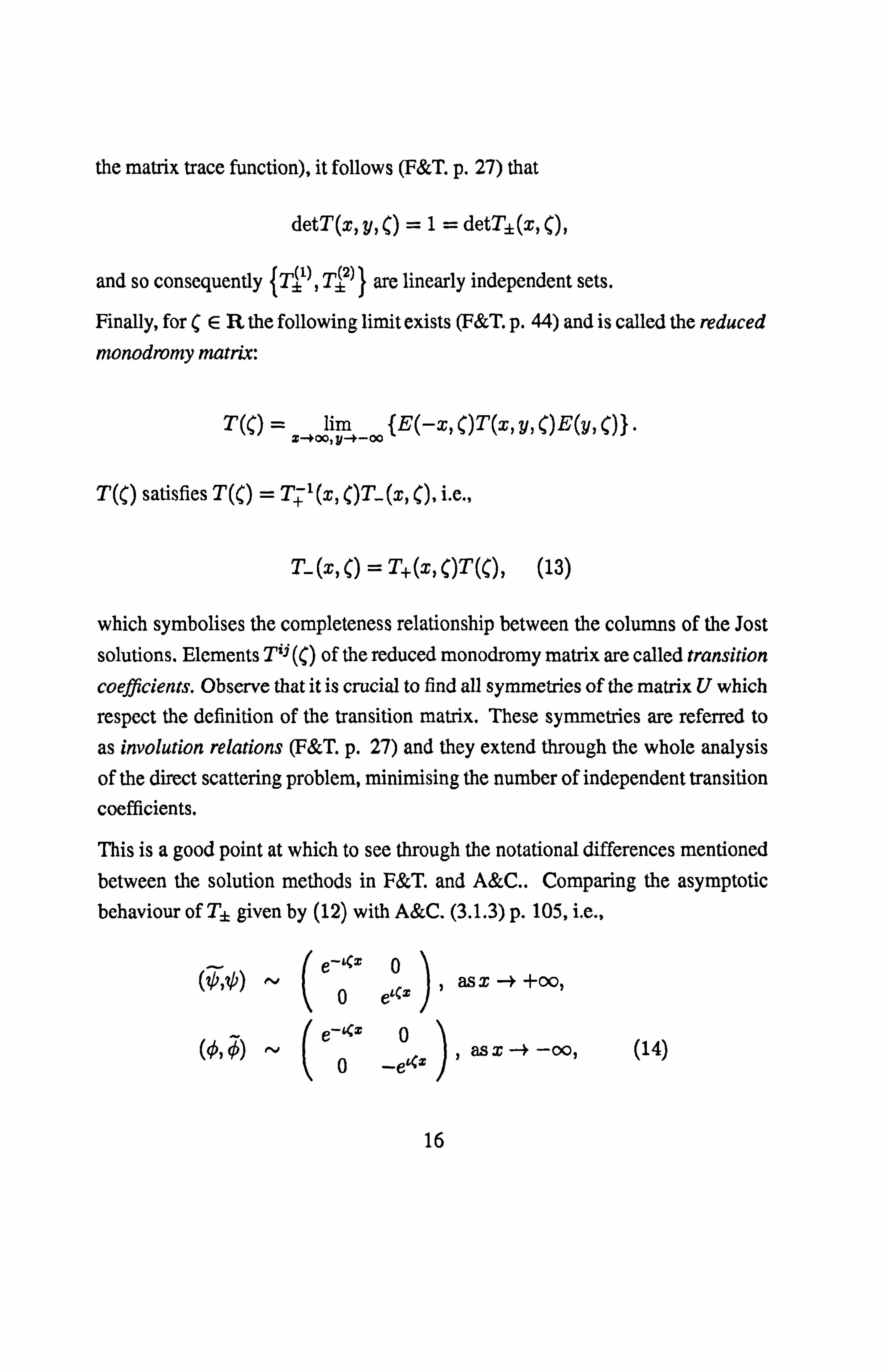
the matrix trace function), it follows (F&T. p. 27) that
detT(x, y, () =1= detT±(x, (),
and so consequently {T'), T 2) } are linearly independent sets.
Finally, for CER the following limit exists (F&T. p. 44) and is called the reduced
monodromy matrix:
T(C) = x-+ýim _ý
{E(-x, ()T (x, y, ()E(y, ()} .
T (C) satisfies T (C) = T+ 1(x, ()T_ (x, C), i. e.,
T_ (x, () = T+ (x, C)T (C), (13)
which symbolises the completeness relationship between the columns of the Jost
solutions. Elements T=j (() of the reduced monodromy matrix are called transition
coefficients. Observe that it is crucial to find all symmetries of the matrix U which respect the definition of the transition matrix. These symmetries are referred to
as involution relations (F&T. p. 27) and they extend through the whole analysis
of the direct scattering problem, minimising the number of independent transition
coefficients.
This is a good point at which to see through the notational differences mentioned between the solution methods in F&T. and A&C.. Comparing the asymptotic behaviour of Tt given by (12) with A&C. (3.1.3) p. 105, i. e.,
^' (ý )
(0, j) ^' ( (
e-K-T 0 , 0 e`cx
as x -+ +oo,
e'Kx 0 , as x --3 -oo, (14)
0 --e`Sx
16
and comparing the relation (13) with A&C. (3.1.4) p. 105, i. e.,
(0, j) _ (Z, o) ab b -ä
' (15)
it is evident that Ablowitz & Clarkson's eigenfunctions 0, ý and 0, ý of d. F = UF simply correspond to the columns of the Jost solution matrices T+ and T_
(albeit the normalisation differs trivially). Note that the use of tildas rather than bars in (14) and (15) avoids confusion with the complex conjugate.
Now that the eigenfunctions required have been characterised, they can be explic- itly found at t=0 by re-expressing the auxiliary differential equation (8) as a
linear integral equation. In fact for our case U= -t( q, the transition r c(
matrix T (x, y, () may be represented as the solution of a Volterra integral equa- tion, whose iterations are of course absolutely convergent. Appropriate limits are then taken in order to obtain integral representations for TT (x, () and T (C) (cf. F&T. p. 30, pp. 39-41, pp. 46-48).
Lastly, analytic properties of the Jost solutions and the transition coefficients, de-
duced from their integral representations, in conjunction with the completeness
relation (13) imply the discrete and continuous spectrum scattering data.
To be more explicit, consider for example the Nonlinear Schrödinger equation dealt with in Chapter 1 of Faddeev & Takhtajan's book ([121), where the matrix U of the auxiliary linear equation has the form
týIX1 O(x) cA/2 t FIX 11,0 (x) cA/2
and the reduced monodromy matrix may be written
T (A) = a(A) -b(A) b(A) -a(. 1)
I
17
Here 0(x) = (x, t= 0) is a known complex-valued function, A is the arbitrary complex parameter, and the bars denote complex conjugation.
In this (generic) case the discrete spectrum data (A complex) comprises:
"A set of discrete eigenvalues {al, ..., A, ti} which are the zeros of the transi-
tion coefficient a(A) in the upper half A-plane, together with their complex conjugates {Xi,
..., "ln}.
" 2n complex coefficients {rye, ryý ja=1, ..., n} called transition coefficients for the discrete spectrum. They are proportionality coefficients existing be-
tween the columns of the Jost solution matrices T±(x, A) at A= a1 and A=T;, i=1, ., n.
Whilst the continuous spectrum data just consists of the set Ib(A), T(A) IA E R}.
(a(A), AER can be expressed in terms of its zeros al, ..., A, a via a "dispersion
relation": cf. F&T. pp. 50-51).
2.1.4 The 2x2 Inverse Scattering Problem.
By taking into account the known analytic properties of TT(x, () and T(C), the completeness relation T_ (x, () = T+ (x, ()T(() will be rewritten and reinter- preted as a vector Riemann-Hilbert problem in scattering space, which can then be formally solved at time t using projections.
Following A&C. pp. 105-109 we suppose the Jost solutions now have the asymp- totic behaviour (14) and satisfy the completeness relation (15). Let N, N, M, .U be the modified eigenfunctions with constant boundary conditions defined by
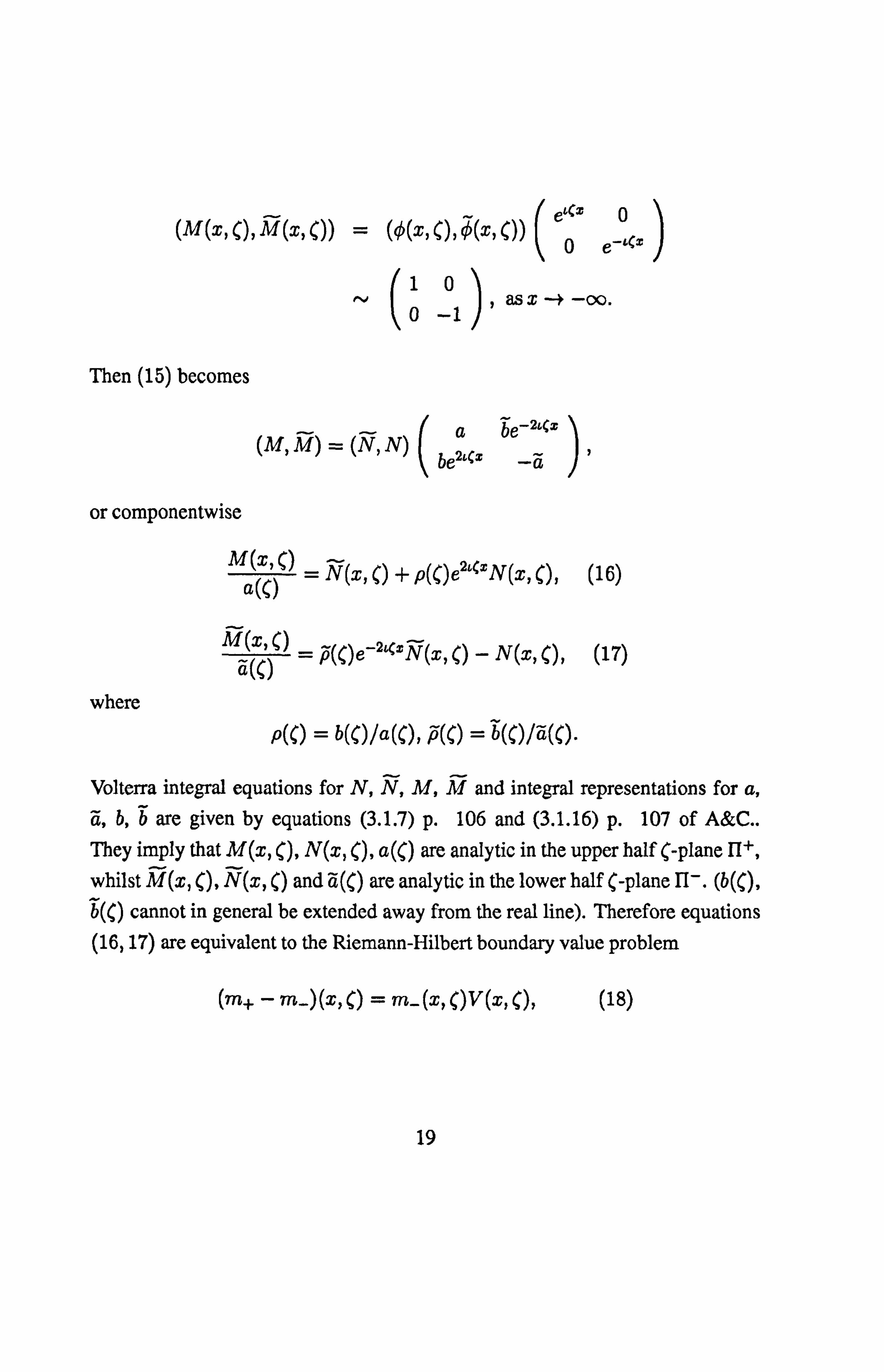
Volterra integral equations for N, N, M, M and integral representations for a, ä, b, b are given by equations (3.1.7) p. 106 and (3.1.16) p. 107 of A&C..
They imply that M(x, (), N(x, (), a(() are analytic in the upper half (-plane lit
whilst M(x, (), N(x, () and ä(() are analytic in the lower half (-plane II-. (b((), b(() cannot in general be extended away from the real line). Therefore equations (16,17) are equivalent to the Riemann-Hilbert boundary value problem
(ý+ - m-) (x, C) = rrc- (x, ()V (x, C), (18)
U eThw
19
where
m+(x, C) =
and
V (X, () = P(C)P(C) P(C)e- 2aSx
P(C)e2iSx 0
N(x, C) , m- (x, () = 1V(x, C), - ä(x, c)
7 (C)
mf(x, () -+ I, as ICI -+ oo.
Suppose that given q(x, 0), r(x, 0) we have solved the linear integral equations for N, N, M, M and hence obtained m±(x, 0, (), the discrete and continuous
spectrum scattering data and V(x, 0, () using (18). Suppose further that we have
found the time dependence of the scattering data from the V-part of the AKNS-
pair. Then the inverse problem requires us to solve the vector Riemann-Hilbert
problem on Im( =0
(m+ - rn-) (x, t, () = rn- (x, t, C)V (x, t, C), rnf(x, t, C) -+ I, as ý(ý -3 00, (19)
finding m± (x, t, () when the matrix function V (x, t, () is known.
For the sake of brevity in this section we assume a((), ä(() have no zeros, mean- ing that mt are analytic rather than meromorphic in their respective half-planes.
In Chapter 5 we will derive a Riemann-Hilbert problem of the same type as (19)
in order to solve the inverse scattering problem for the RMB-system, and we shall
explicitly carry out the extra calculations demanded by allowing meromorphic
m}.
Define the projection operator P} by
1ýu ýP±f ý (C) - 27r6 foo
u- (ý f L0) du. (20)
20
If ff (() are analytic in IIf, and f±(() -+ 0 as I(I -4 oo, then it is immediate
using Cauchy's Integral Formula from Complex Analysis that
Alternatively, another asymptotic expansion for m_ in inverse powers of C is
gained simply by using integation by parts, the rapidly decreasing boundary con- ditions for q and r at infinity, and the integral representations for N, M and ä. In fact
1+ 2K f' q(C, t)r(C, t)dý 2i(Entl < M- (X, t, () N > 71C 1+ 2LS f xI q(e, t)r(E, t)d
as 1(1 -p oo, which upon matching coefficients of C-' in the (1,2) and (2,1)
positions gives
q(x, t) =
r(x, t) =
_1 %O0
-2aux J oo
p(t, u)e Nl (x, t, u) du,
1 %O0 2ýux ýfý
p(t, u)e N2(x, t, u) du,
where Nl is the (1,1) element of N, and N2 is the (2,1) element of N.
21
Evidently these formulae describe q and r at a general time t in terms of the continuous spectrum scattering data (i. e., p(t, (), p(t, () which are known) and the solutions m± of (19) (i. e., N(x, t, (), N(x, t, ()).
2.2 BäckIund and Darboux-Bäcklund Transforma- tions.
In this section we review two allied methods for calculating pure multi-soiiton solutions to integrable nonlinear PDEs.
2.2.1 Bäcklund Transformations.
A Bäcklund transformation is a system of equations which implicitly defines a mapping between local solutions of either two different partial differential equa- tions or one single partial differential equation.
More precisely, given two uncoupled partial differential equations P(u) = 0, Q(v) =0 for u= u(x, t), v= v(x, t), a Bäcklund transformation may be defined [25] as a pair of relations
2 ý(u, voux, vx, ut, vt, ...; x, t) = 0,2 = 1,
satisfying the following property: if u is chosen to be a solution of P(u) = 0, then R; =0 are integrable for v and the resulting v is a solution of Q (v) = 0, and vice versa. If the operators P, Q are the same, then 0, i=1,2 are called an auto-Bäcklund transformation.
It is intriguing that every evolution equation solvable by the IST has its own auto- Bäcklund transformation. Moreover, the AKNS-pair corresponding to a particular integrable equation itself represents a Bäcklund transformation: cf. Ablowitz and Segur [26] pp. 156-157.
22
Suppose now that P(u) 0 is an integrable PDE with AKNS-pair
8j = U(u)F,
ätF =VF.
Then applying the auto-Bäcklund transformation for P(u) =0 to a given (suitably
behaved) solution uo(x, t), P(uo) = 0, yields a new solution ul(x, t), P(ul) =0 characterised by the fact that the spectrum of OF = U(ul)F differs from the
spectrum of OF= U(uo)F by exactly one discrete eigenvalue. Consequently, if
ua is an n-soliton solution, then ul will be an (n ± 1)-soliton solution. A standard trick for obtaining 1-solitons is therefore to apply the auto-Bäcklund transforma-
tion to the trivial zero solution of P=0 (providing of course P=0 possesses this
solution). Higher order solitons are then found either by further applications of the Bäcklund transformation, which unfortunately requires repeated integrations,
or preferably by algebraic means alone if the Bäcklund transformation satisfies a
permutability theorem. We shall demonstrate this method with a typical example for finding a 2-soliton solution of the sine-Gordon equation
uxt = sin u.
An auto-Bäcklund transformation for the sine-Gordon equation is given by
(u - v)x = 2a sin[(u + v)/2], (u + v)t = 2a-1 sin[(u - v)/2],
where a 36 0 is an arbitrary constant. (As can be verified by cross-differentiation). If we choose
v= vo with (vo)xt = sin (vo) ,
and if we successively take a= ai (i = 1,2) in the Bäcklund transformation, then by definition we obtain two solutions u= vi (say) of the sine-Gordon equation.
23
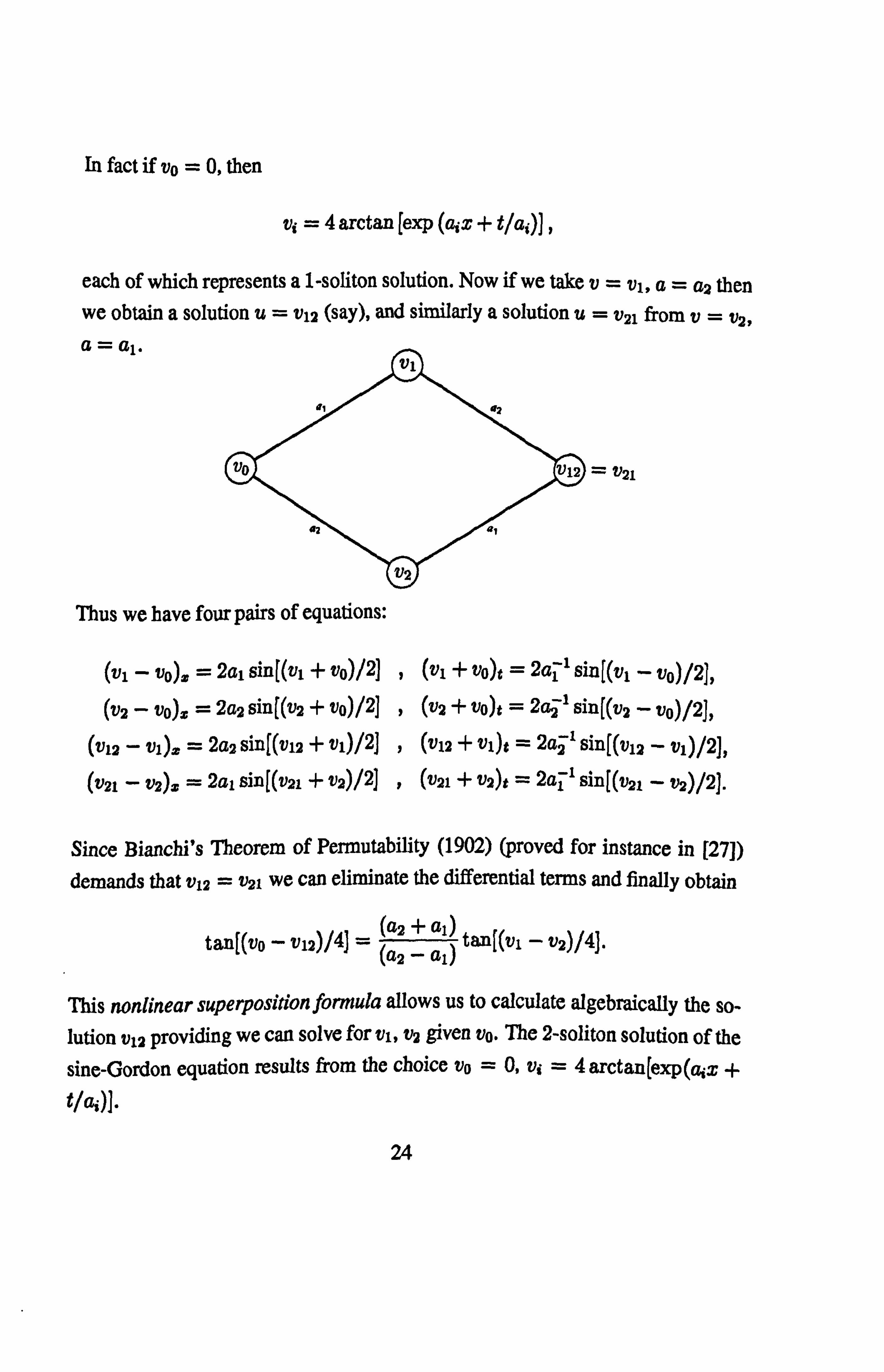
In fact if vo = 0, then
v, =4 arctan [exp (a; x + t/as)] ,
each of which represents a 1-soliton solution. Now if we take v= vi, a= a2 then we obtain a solution u= v12 (say), and similarly a solution u= v21 from v= v2, 3= a1.
Since Bianchi's Theorem of Permutability (1902) (proved for instance in [27]) demands that v12 = v21 we can eliminate the differential terms and finally obtain
) tan[(vl - v2)/4]. tan(((/vo - v12)/4] _ (a2-
-
al) l
This nonlinear superposition formula allows us to calculate algebraically the so- lution vie providing we can solve for vi, v2 given vo. The 2-soliton solution of the
sine-Gordon equation results from the choice vo = 0, v; =4 arctan(exp(a; x + t/a; )].
24
It is straightforward in principle to continue this process, although the calculations become very involved for large n. The sequence of Bäcklund transformations leading to a 3-soliton solution v123 is illustrated below:
V123 = V213 = V231 etC.
2.2.2 Darboux-Bäcklund Transforms.
A Darboux-Bäcklund transform is a special type of gauge transformation which can be used to effect auto-Bäcklund transformations between n and (n+l)-soliton
solutions of integrable PDEs.
Let M(q) =0 be an integrable nonlinear system for an unknown vector function
q(x, t) = (ql,..., q,. ) (x, t), N9r>1, and let
F. = U(q, ()F, Ft = V(q, C)F
be the associated AKNS NxN linear system.
25
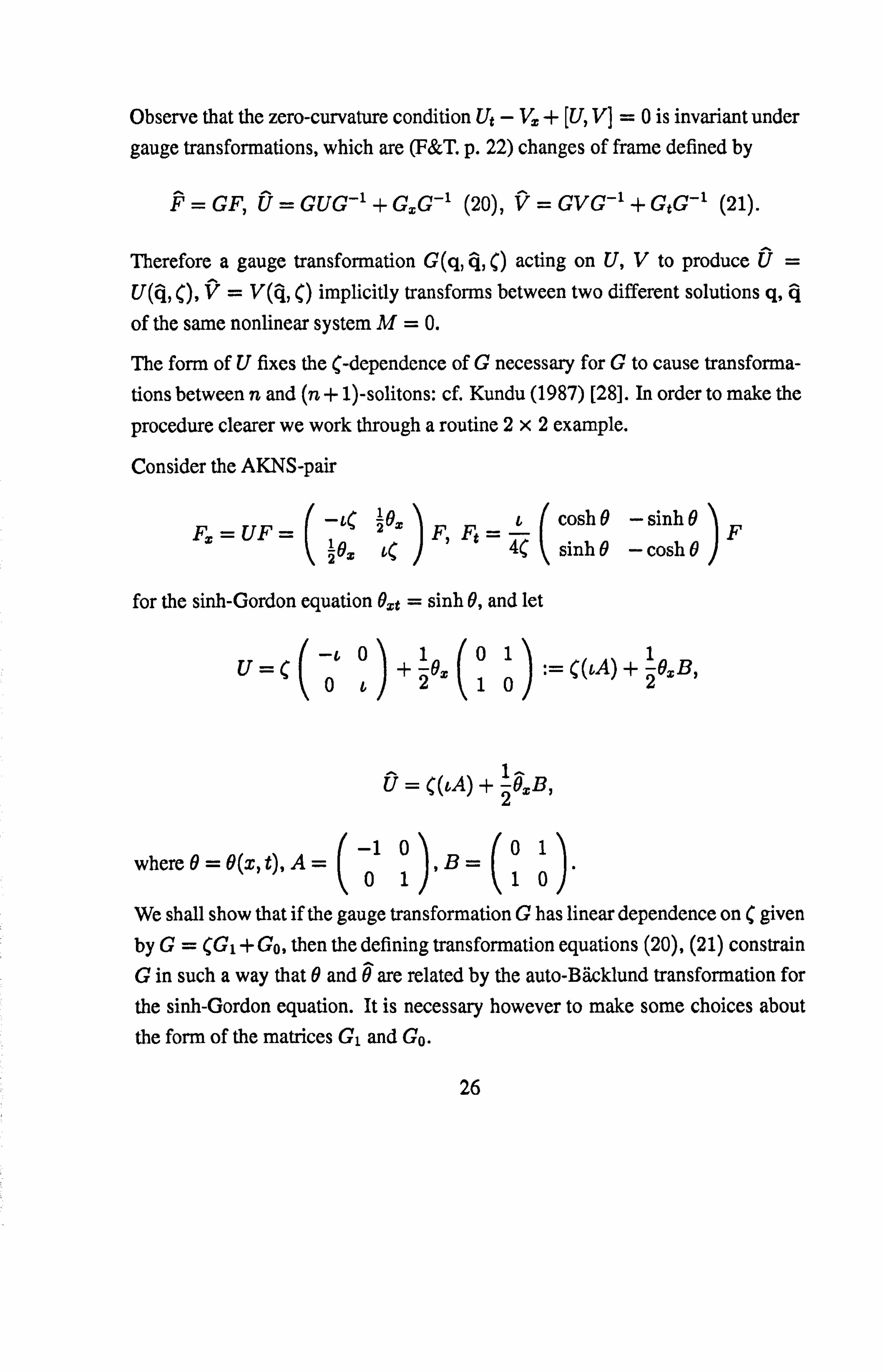
Observe that the zero-curvature condition Ut - Vx + [U, V] =0 is invariant under gauge transformations, which are (F&T. p. 22) changes of frame defined by
Therefore a gauge transformation G(q, q, () acting on U, V to produce Ü=
U(q, (), V=V (q, () implicitly transforms between two different solutions q, q
of the same nonlinear system M=0.
The form of U fixes the (-dependence of G necessary for G to cause transforma-
tions between n and (n + 1)-solitons: cf. Kundu (1987) [28]. In order to make the
procedure clearer we work through a routine 2x2 example.
Consider the AKNS-pair
F UF FF-c cosh B- sink BF F--
2 8x ,t 4( sinh 0- cosh 0
for the sinh-Gordon equation 8xt = sinh 0, and let
U=ý -c 0+ 19y 01 . -C(bA)+
19. B,
Oc2102
U= C(tA) + 2eý, B,
where 0=6(x, t), A= -1 0 , B=
01 0110
We shall show that if the gauge transformation G has linear dependence on C given by G= (Gl +Go, then the defining transformation equations (20), (21) constrain G in such a way that 0 and B are related by the auto-Bäcklund transformation for
the sinh-Gordon equation. It is necessary however to make some choices about the form of the matrices Gl and Go.
26
Substituting for G, U and U in (20) we find that the quadratic polynomial
0= {2 11-
[G1, cA]+Gly+OXG1B-20,, BG, +[Go, tA]}+
Go, +2OG,, B-2OBGo
must be satisfied identically in (.
A suitable choice for Gi is Gl = aA, (G1 oc I also works), and if we write ab G° cd,
then by equating the coefficients of C and CO to zero we obtain
b=c=1 (8 + g)x (22)
and
a=d,
ax =Z b(B - 9)x, (23)
bx _2a (B - B)x, (24)
respectively.
Now suppose that a=a (B2 B),
and define f=f (B20)
with f=a. Then from
equations (23,22) we have that
a'=b=4(9B)x =. f",
whilst equations (24,22) give 1 (9 + 9)xx = fx, i. e.,
4 (9
(taking the integration constant to be zero). Therefore f= f", which has a solu-
27
tion
With
f
fl =a=d=ýcosh 9B
2)
K sinh 9-
28
b=c=4(B+9) ý x
I
where ic is an arbitrary constant parameter. In particular, upon resealing 0= 0/2, ý= B12, we have the x-part of the auto-Bäcklund transformation
(0 + 0)�� = 2r. sinh(iß - 0).
The t-part of the Bäcklund transformation, namely
(ý - 0)t = 2ý sinh(j + 0),
ensues by substituting for V and G in equation (21).
Our example has shown how a Darboux transform acts in an equivalent way to
an auto-Bäcklund transformation. Multi-soliton solutions are found just as for
Bäcklund transformations: the Darboux transform is applied to the trivial zero so- lution of the nonlinear system in question, then higher order solitons are calculated
algebraically where possible using a permutability theorem.
28
Chapter 3
Formulation and Integrability of the 3-Level Maxwell-Bloch Equations.
Consider the system consisting of an electromagnetic plane wave interacting with a uniform dielectric of 3-level quantum-mechanical atoms. It is assumed that the
atoms are rotationally symmetric in the transverse plane. The equations modelling this system can be written:
ýý. atr = [x, rý , aZA-C-2 at2A = -C
2E01 atP.
The first equation is the Liouville equation of motion for the 3x3 quantum density
matrix r. The second is Maxwell's equation, where A(z, t) is the vector potential field of the plane wave, P(z, t) is the polarisation density induced in the atomic ensemble, and c is the speed of light in vacuum.
By definition the density matrix r is hermitian and has the property Trip = 1. However the form of the Liouville equation permits us to define a new traceless
29
density matrix p through the relation
r= 3ý + 2P
where I= diag {1,1,1}. Clearly p also satisfies the Liouville equation
thatP = [H, PI " y
'IN Upper
y- energy level. (Direction of propagation. )
---"> x
Upper x-energy level.
If we suppose that the atom-field coupling is minimal-replacement [29], then the Hamiltonian matrix H takes the form
where h 10 is the energy level of the orthogonal x and y states, the momentum operator is given by
p= (t'bP2)P3) _(x
0 -c 000 -c 100, py 000 000c00 (
and -e, m are the charge and mass of the electron respectively.
30
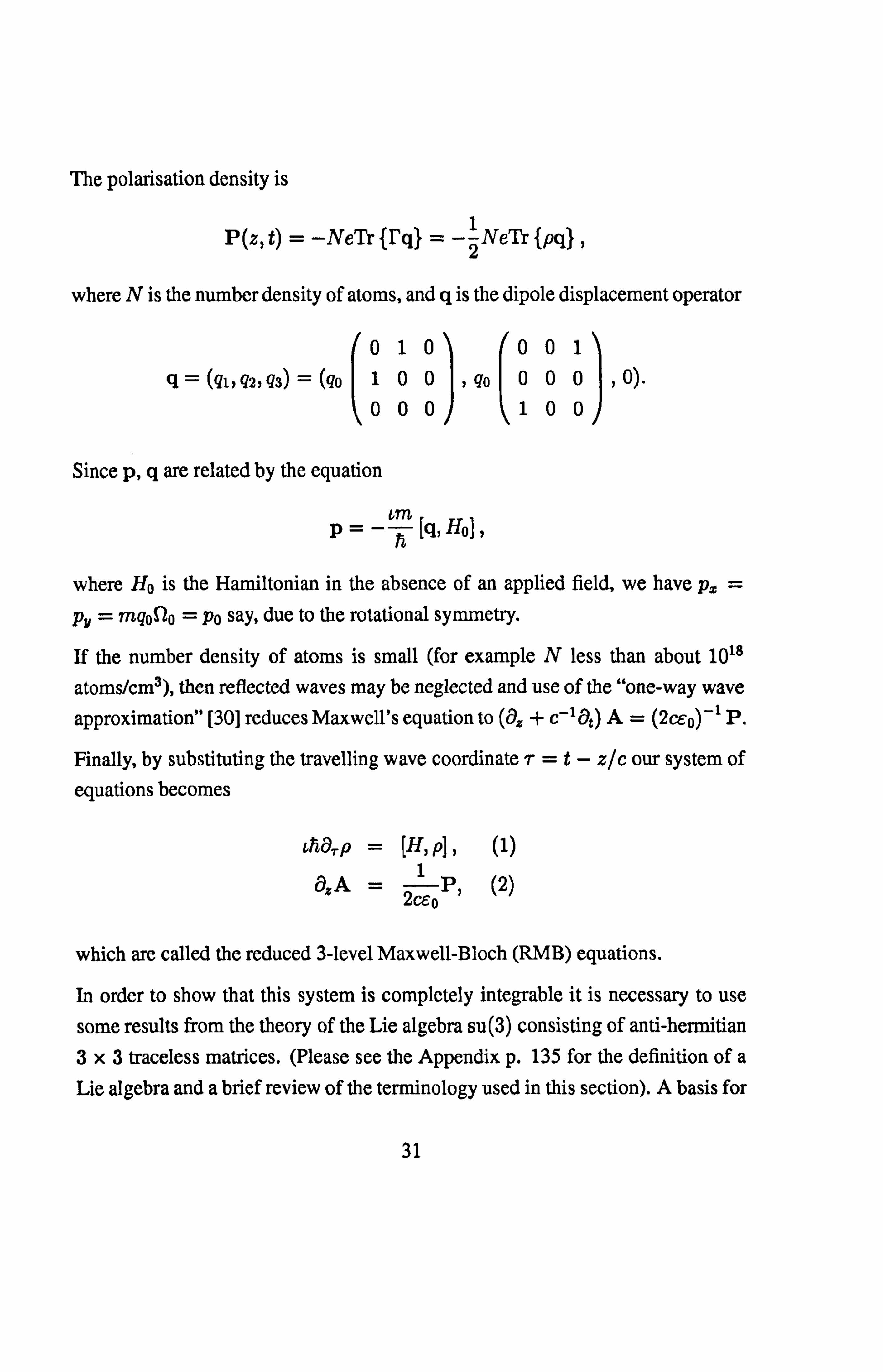
The polarisation density is
P (z, t) = -NeTr {I'q} 2 NeTr { pq} ,
where N is the number density of atoms, and q is the dipole displacement operator
010001 / Q=ql, q2, (73) = (g0 100, q0 000,0).
000100
Since p, q are related by the equation
P=- bý [q, HoJ ,
where Ho is the Hamiltonian in the absence of an applied field, we have px =
py = mq0 Zo = po say, due to the rotational symmetry.
If the number density of atoms is small (for example N less than about 1018
atoms/cm3), then reflected waves may be neglected and use of the "one-way wave
approximation" [30] reduces Maxwell's equation to (ö + c-18t) A= (2ceo)-1 P.
Finally, by substituting the travelling wave coordinate r=t- z/c our system of
equations becomes
ahäTP = [H, p], (1)
ÖzA 2ýoP'
(2)
which are called the reduced 3-level Maxwell-Bloch (RMB) equations.
In order to show that this system is completely integrable it is necessary to use
some results from the theory of the Lie algebra su(3) consisting of anti-hermitian 3x3 traceless matrices. (Please see the Appendix p. 135 for the definition of a Lie algebra and a brief review of the terminology used in this section). A basis for
31
su(3) is the set {-tA 1/2, ..., -tAs/2} such that
010000
Jý1= 100 , a2= 001
000010
0 -c 0000 A4
=L0 0Ag =00 -6
000060
i0olo A7 =0 -1 0 I, 8ZI =
in 01
001 A3= 000
100
00 -c as =000
600 ý I
0 I, (3-10)
10 0 0ý ' `0 0 -2
with structure constants f147 = 1,
f135 = 1126 = 1432 = 1465 = 1376 = 1572 =-21
ýýý 1368 = 1258 =
satisfying 8
2'
2c E fjkt, \, j = (Ak, 1\1] . (11)
j-1
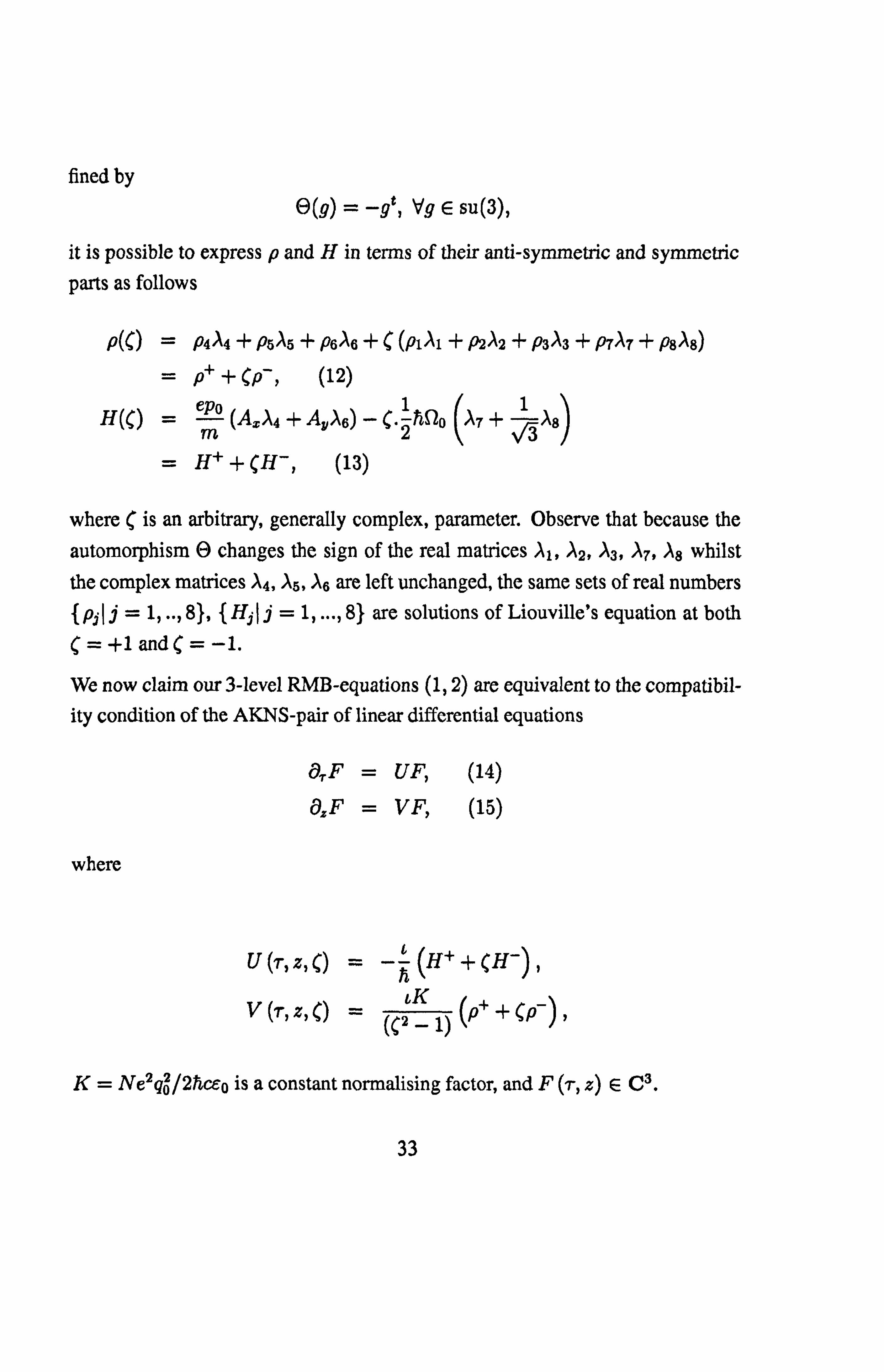
p and H, being hermitian traceless matrices, can therefore be written
where S is an arbitrary, generally complex, parameter. Observe that because the
automorphism O changes the sign of the real matrices Al. A2+ A39 A7, )ºg whilst the complex matrices A4, A5, As are left unchanged, the same sets of real numbers { p3 Ij=1,
.., 8}, { H3 j=1, ..., 8} are solutions of Liouville's equation at both
(=+l and(=-1.
We now claim our 3-level RMB-equations (1,2) are equivalent to the compatibil- ity condition of the AKNS-pair of linear differential equations
OF = UF, (14)
8zF = VF, (15)
where
U (, r, z, () =- ý6 (H+ + (H-),
V (T, z, () = (ýGK1) `P++(P )2
K= Ne2gö/2hceo is a constant normalising factor, and F (7-, z) E C3.
33
In fact, forming the zero-curvature condition (cf. equation (3), p. 11)
00U-OTV+[U, V1 =0,
and multiplying throughout by hK'1 ((2 - 1) gives
0= b2 (_oH + [H_, p ]) +( (-tharp- + [H+, P ]+ [H p+]) +
chap++ Ka, H++ [H+, P+1)
The Fundamental Theorem of Algebra then implies that this quadratic polynomial in ( will be satisfied identically for all CER if it is satisfied at three distinct values of C, which are taken to be (= oo and (= ±1. At these values we find
öxH+ _ -aK [H-, PJ, (16)
cýiäT ýP+ ýPl= [H+ ±H-, p+ ±P ]" (17)
Equation (17) is evidently just the same as Liouville's equation (1). Moreover
calculating the commutator [H-, p-] using (3 - 10), (12,13), and then matching coefficients of A4 and A6 in equation (16), leads to
Kh Nego ÖA, = --pl pl,
eqo 2c¬o Nego ÖzAy par 2ceo
which are exactly the components of the Maxwell equation (2).
Comparing the AKNS-pair (14,15) with the generic AKNS-pair (1,2) on p. 11
we see there is a simple yet important difference. Namely, for the 3-level RMB-
system it is the propagation distance z, rather than time t, which is to be thought of as the evolution variable, and the transverse variable is the shifted time r= t-z/c,
as opposed to x. This is a common occurence in optical applications where the initial input pulse at z=0 is known as a function of time, and then the output
34
pulse is detected at some z>0 and again determined as a function of time.
We conclude the present chapter by specifying the initial value-boundary value
problem for the RMB-equations. Componentwise the RMB-system (1,2) be-
comes
aTPI = SZo [e-qo (2A. ýP7 - AbP2) + P4] 0oeqo
aTPa =h (A., P3 + Aypi) ,
arPs = SZo (eý [-AýPa + AY (P7 + V3-p8)] + p6},
07-P4 = 00 (h
AYPS " PlJ
OoeQo aTP5 =
,ý (AxP6
- AYP4) ,
aTps aTP7
aTp8 ÖxAx
2 (Ap5
-+ P3 1e
_ PoeQo
(2AxPi + AyPs) i h
-\, F3Qoego AyP3) (18-25)
h
- Neqo
Pi ' azAy =- 2ý
o Ps. (26,27) 20 0
i. e., ten first order nonlinear PDEs for the ten unknown functions Ax, Ay, p1,..., p8
of two variables r, zE (-oo, oo).
We prescribe Ax, Ay on z=0, subject to boundary conditions of rapidly de-
creasing type. If we choose A,, (r, 0) = Al (r), Ay (T, 0) = A2 (T) to be known
functions of r, then equations (18 - 25) on z=0 represent a system of ODEs
which can be solved uniquely for pl, ..., p8 (r, 0) as functions of A1, A2 (T), as-
suming that p1i ..., p6-+0, p7 ->1, p8 -+ 1//, as tTI -3 oo. Ax, Ay are
supposed to be infinitely differentiable and together with all their derivatives to decay faster than any power of ITI-1 as 17-1 -+ oo.
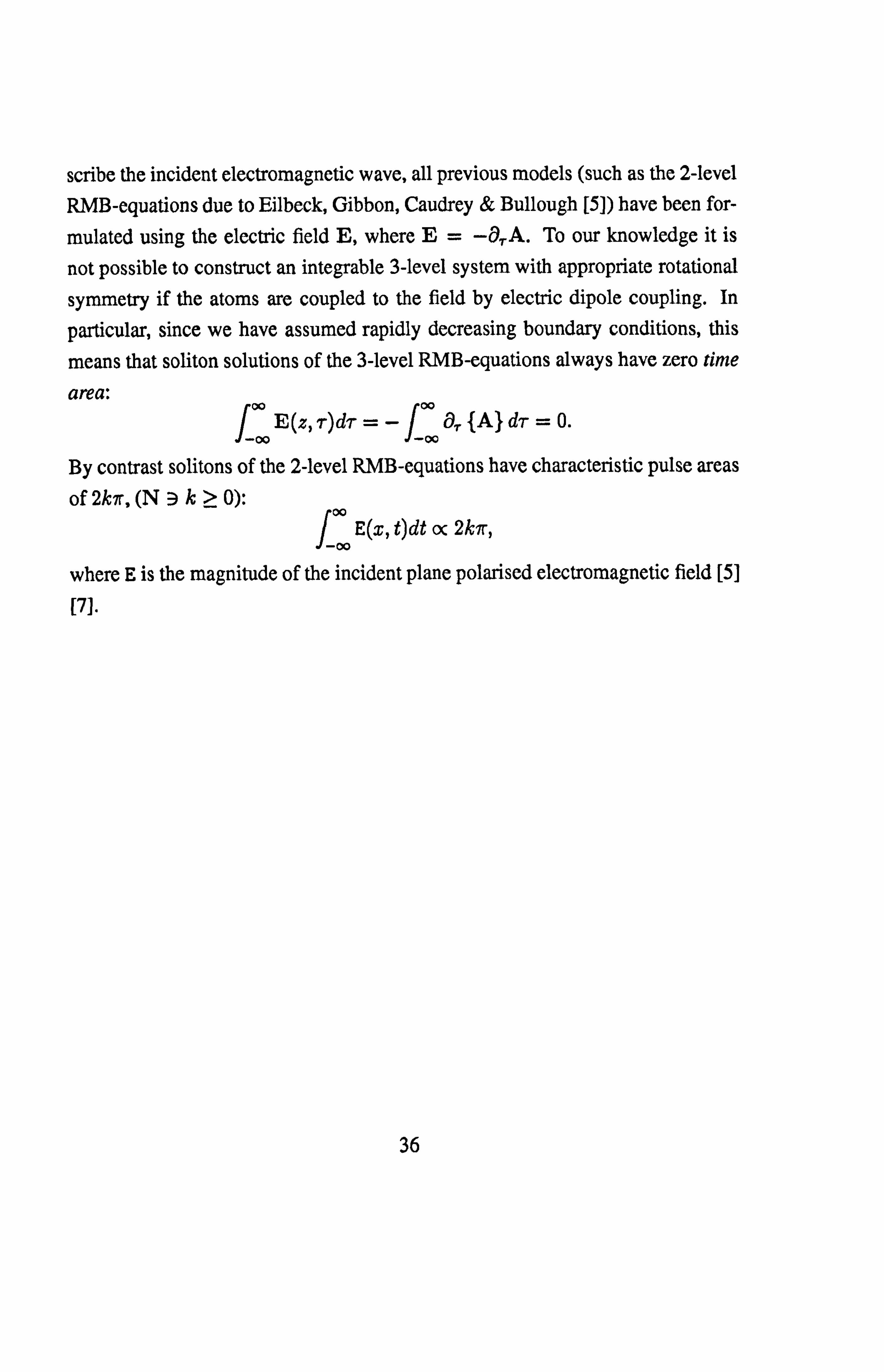
It is worth emphasizing that whereas we have used the vector potential A to de-
35
scribe the incident electromagnetic wave, all previous models (such as the 2-level
RMB-equations due to Eilbeck, Gibbon, Caudrey & Bullough [5]) have been for-
mulated using the electric field E, where E= -OVA. To our knowledge it is
not possible to construct an integrable 3-level system with appropriate rotational
symmetry if the atoms are coupled to the field by electric dipole coupling. In
particular, since we have assumed rapidly decreasing boundary conditions, this
means that soliton solutions of the 3-level RMB-equations always have zero time
area:
j°°E(z, r)dr=-f 00
ä., {A}d7- =0.
By contrast solitons of the 2-level RMB-equations have characteristic pulse areas
of 2kir, (N Dk> 0): f
000 0 E(x, t)dt a 2kir,
where E is the magnitude of the incident plane polarised electromagnetic field [5]
[7].
00
36
Chapter 4
Use of Darboux-Bäcklund
Transformations to find Fully
Polarised Soliton Solutions.
Chapter 4 is divided into two sections. In the first section we calculate the fun-
damental single soliton expressions for A.,,, Ay and additionally for the density
matrix components pl, ..., p8. Taking into account our previous discussion of Dar-
boux transforms (pp. 25-28) a gauge transformation G= CI + X, linear in the
parameter (, will be used to generate these solutions. However, determination of the correct form for the matrix X is a difficult problem as we are now dealing with
a 3-level system. Following Arnold [8], and motivated by the work of Park & Shin
[9] [10], we shall see that defining X in terms of a hermitian projector matrix G
proves successful. In Section 4.2 sequences of two one-parameter Darboux trans- forms are applied in conjunction with a nonlinear superposition formula to obtain both linearly polarised and elliptically polarised 2-solitons of the RMB-equations.
Our formulae specifying the elliptically polarised solitons are the primary results here, they are previously unpublished and represent a natural vector generalisa- tion of the modulated 07r-pulse solutions of the 2-level RMB-equations derived
37
by Bullough, Caudrey, Eilbeck & Gibbon [5] [7].
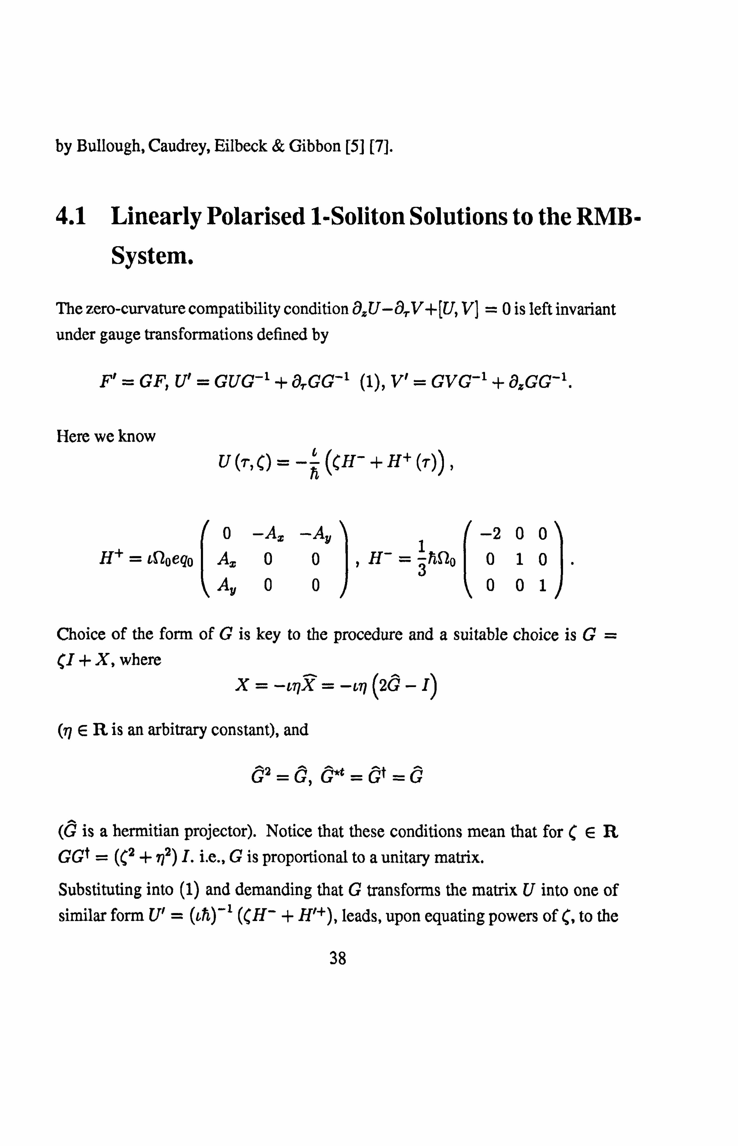
4.1 Linearly Polarised 1-Soliton Solutions to the RMB- System.
The zero-curvature compatibility condition äzU-ä, V+[U, V] =0 is left invariant
under gauge transformations defined by
F' = GF, U' = GUG-1 + 0TGG'1 (1), V' = GVG-1 + a, zGG-1.
Here we know U ((H- + H+ (T))
0 -Ax -Ay -2 00 H' = aSZoego Ax 00, H- = 3ho0
010 Ay 00001
Choice of the form of G is key to the procedure and a suitable choice is G=
(I + X, where x= -07X = -cry 2G -I
(77 ER is an arbitrary constant), and
o2=6, O*t=Gt=G
(G is a hermitian projector). Notice that these conditions mean that for (ER GGt = ((2 +, n2) I. i. e., G is proportional to a unitary matrix.
Substituting into (1) and demanding that G transforms the matrix U into one of similar form U' = (th)-1((H' + H'+), leads, upon equating powers of c, to the
38
equations
H'+ - H+ = [X, H"],
ttxXz = H'+X -X H+,
0 -A' -A' where H'+ = tgoego A' 00
A'y 00
The simplest 1-solitons are generated by our Darboux transform acting on the zero field solution to the RMB-system. Therefore we take H+ = 0, giving
H'+ ~ [X, H ], (2)
chXT = H'+X (3)
Using equation (2) and the condition G2 = G, we find G may be written as follows
1t sst G= -ss =, 9 sts
9
s= CAx/2r1 CA'y/2r1
where g2 -g+ QC2r'2 (A'2 + Ar2) = 0, and C := eqo/h. (Providing s is real
valued, G satisfies Gt = G).
Equation (3) can now be integrated yielding g and the components A', A' of the
transformed field. In fact (3) implies
9z = 2Q0q9(9 - 1),
A' XT = S2on(29 - 1)Ax,
AýT = SZoý(29 -1)Ay,
with g (g -1) >0 and g (g -1) -3 0, as Jr I -+ oo, since A. ',, A'y -+ 0, as Jr I -+ oo.
39
Hence
g e2e + 1,
Ax =C sechB, Aý =C sech9,
where 0= Qorl (T - ro), and the constants a, b must satisfy a2 +b2 =1 for
consistency.
A', A' are real provided that the arbitrary constants a := cos ¢, b := sin q5, and To are also real numbers.
of the RMB-system, whose polarisation direction lies at an angle 0 to the x-axis,
are generated from the zero solution by the Darboux transform G= (I - cr79 = ((+ cry) - 2ti O, where the real symmetric projection matrix 0 is given by
sst 11 G_ 1e sts,
s= e29+ae ý
beB
a2+b2= cos20 +sin20 = 1.
The z-dependence of the parameter To = To (z) will be found presently.
where M(ij) denotes the (i, j)-th element of a matrix M. This makes it possible to read off the fields A', A' once the Darboux matrices Xl and Y2 are found.
Now suppose the parameters associated with the matrices Xj are defined to be
77j, a1 = cos ¢j, b1 = sin Oj, Bj =I oqj (T - r3), j=1,2. From the equality
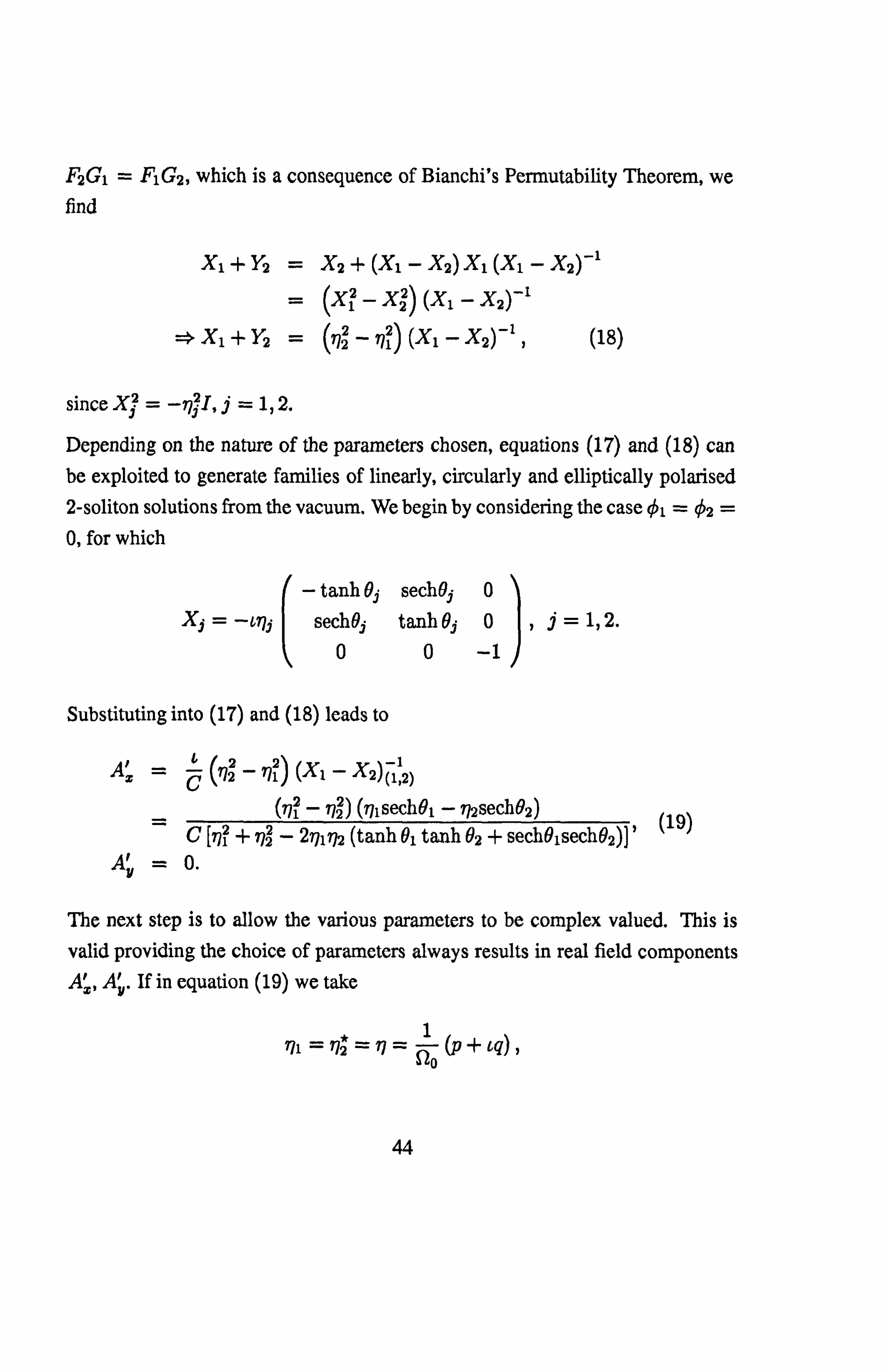
43
F2G1 = F1G2, which is a consequence of Bianchi's Permutability Theorem, we find
XI + Y2 = X2 + (Xl - X2) Xl (Xl - X2)-1
_ (XL - X2) (Xl - X2)-1
z* Xl + Y2 = (772
- 771) (Xl - X2)-1
3 (18)
since Xj = -raj I, j =1,2.
Depending on the nature of the parameters chosen, equations (17) and (18) can be exploited to generate families of linearly, circularly and elliptically polarised 2-soliton solutions from the vacuum. We begin by considering the case 01 = 02 = 0, for which
The next step is to allow the various parameters to be complex valued. This is
valid providing the choice of parameters always results in real field components A', A',. If in equation (19) we take
rli =7lä ý_ (P+ýq)
44
and
el = e2 = n077 (T - T1)
= P(T -W)+tQ(T-ýP)ý (say)
then at W= ip =0 we have
A' 2psechpT [cos qT - (pq-1) sin qT tanh pr] 20 x SZoC [1 + (p2q-2) sin 2 grsech2pr]
()
A'y = 0.
(Replacing pr by p (T - cp) and qr by q (r - ii) gives the correct formula when cp, cp & 0). Below there is a plot of Sl0CA' as a function of r when p=1 and q=4: nQCAz
Expressions (19) and (20) both represent linearly polarised "breather" solitons having zero time area. They may be rotated to any given direction of polarisation by applying a r-independent gauge transformation R so that G i-+ RGR-I, where
100 R := exp (c¢. 5) =0 cos q5 sin ¢, q5 E R.
0- sin 0 cos qS
45
Let us move on to the problem of constructing elliptically polarised solitons. In
order to guarantee the reality of Ax, A'' we require
Then
which is pure imaginary, and
Xi-X2
Hence
)' '72 = 71, and G1 = G2* = G.
4tpq Sl' 0
-26 (77161
- 7I2G2) +L (7I1 - 772) I
-2c (770
- ý*G*) +c (77 - ý*) I
o {-2c [(p
-}- ig) G- (p - cq) G*, - 2qI }ER. (21)
A'x =ýpC (Xi - X2)112) E R, A'ý, _ýoC (X, - X2)113) E R.
It remains to find the inverse of Xl - X2, only this time we will permit complex
parameters a and b. Our task is simplified by first refining the form of G.
In the previous section we showed that
1 G=st, 1
aee , where a2 + b2 = 1. sts e28 +1
bee
e-e Equivalently, dividing the original s by 2sechO,
G is generated by a, which b
bee
46
e'n0nT in turn can be rewritten as s= ka ,C3k constant, by rescaling.
kb In fact
) e-nOn(T-T)
=k a b
1 HkIaI, scaling out T= -� In k.
e-no+! '+'
a b
Suppose we choose the case a= cosh 0, b=t sinh 0, k= sechq5,0 E R. Then ka = 1, kb = tT, where T := tanhqS, f=- (2S2oi)-l In (1 - T2),
B (p+iq) r
s= 1
cT
and
e-no+P+ ke-'1on'r ka =ka kb b
[e-ikp-"")T +I -i `j J.
_,.,,, I -(n+ig)T 1 c"i
I
ý
e 2(P+cq)T -(P+iq)z cT e-(P+q)T e-(P+iq)T 1 cT
6T e (P+aq)r tT -T2 cTe (P+, g)T tT -T2
Finally, substituting for d and G* in equation (21) and inverting the resulting expression for X1 - X2 gives
A, _ 4pe pT {2T2p2 cos qT + pq sin qr [e-2pr - (1 - T2)] + q2 cos q7- [e-2p'' + (1 + T2)]}
Y S20C tq2 (e-2p7' + (1 + T2))` + 4p2 le-2pT (sin' qT + T2 cos2 g7-) + T21 j 4pTe PI {-2p2 sin qT + pq cos qr [e-2pr + (1 - T2)] - q2 sin q-r [e-2pr + (1 + T2)]}
a co71 bI-.
47
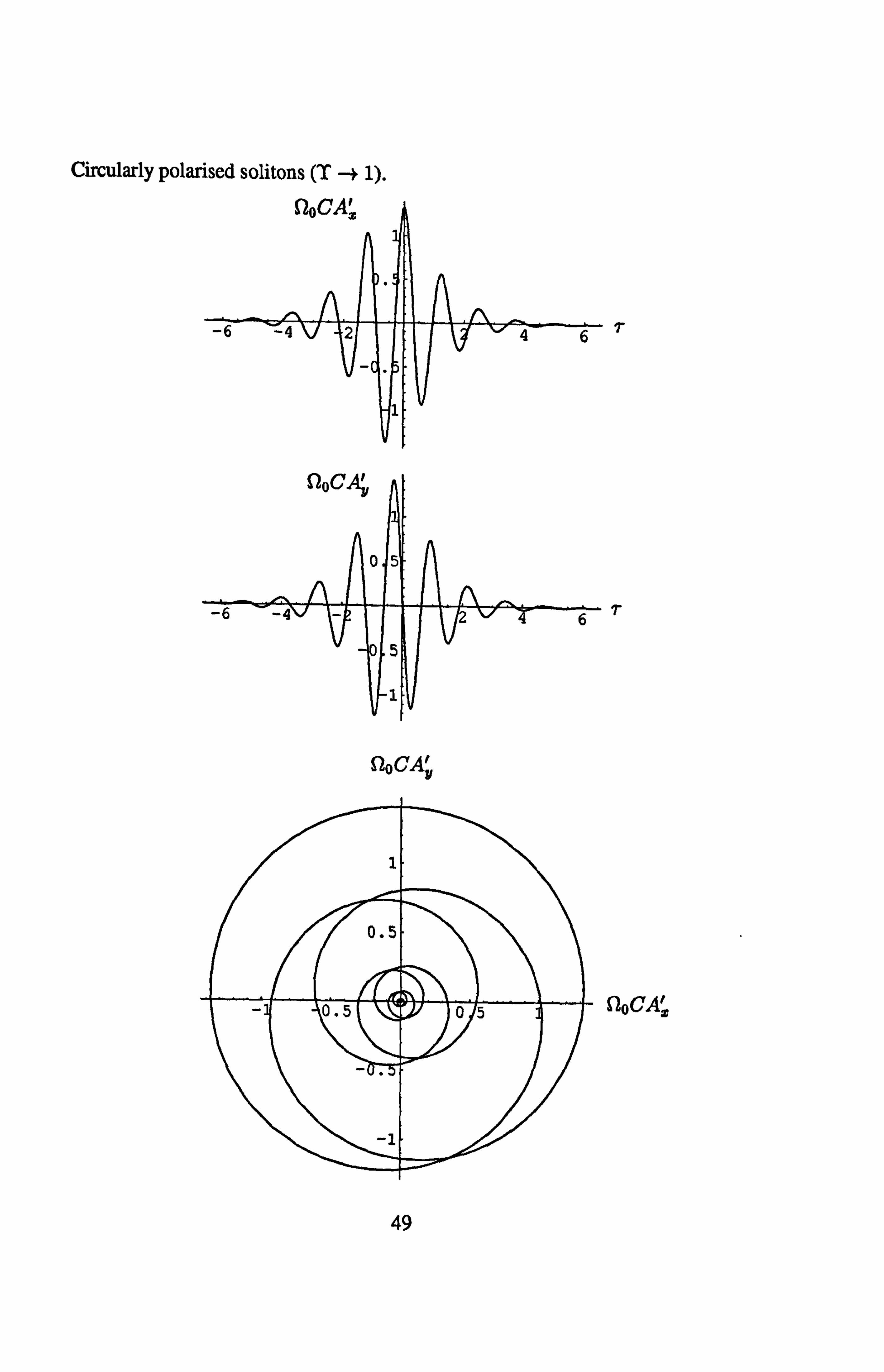
Circularly polarised solitons correspond to the limiting case T -+ 1 (or T --> -1), when we have
A, _ 4pe-PT [2 (P2 + q2) cos qT + qe-2PT (q cos qT +p sin qr)j
10C [q2e-4PT +4 (p2 + q2) (e_2PT + 1)] I
A' _ 4pe-p'' [-2 (p2 + q2) sin qr + qe-2Pr (p cos qr -- q sin qr)]
y Sl0C [q2e-4Pr +4 (p2 + q2) (e-2Pr + 1)]
Using partial fractions and the identity
f1 (pr+1n ý) sech ,z= e-2pr, z+ A 27A
leads to
A, _P [q cos gT +(00177I + p) sin gT]
sech [pr
+ In 2 0In I (Q01, q 1+ P)
x ýoc ýMo 17711 (CQo 1771 +ý) q
+ [g cos gT - (sto 1771 - p) sin gT] sech
[P7-
+ In '2F1101771 (11o I7,1 - P)
, 2Q01711(Q0 li7l - p) q
A' v
p[-gsin gT +(Qo IqI + P) cos gT] sech + In 2SZo In7I (lQlo IrjI + P)
pr 5oC 2s-to IýI (ýo Iýl +rý) q
[g sin gT + (Qo Ir%I - p) cos qT]
sech lp
T+ In J2 "o IýI (" 0
I, qlI - lp') 2Sto 1771 A 1771 - P) q
There follow some illustrative graphs of the transformed field components in the
case p=1, q=5:
48
Circularly polarised solitons (T -* 1). 1oCAy
StoCA'y
SZOCAx
49
Elliptically polarised solitons for the case T= 1/2.
SZOCA'x
SZoCA' y
50
Chapter 5
Inverse Scattering for the RMB-System.
We proceed to solve the initial value-boundary value problem (stated on p. 35) for
our RMB-equations by means of the inverse scattering transform method.
Consider the 3x3 AKNS-pair corresponding to the RMB-system which from
p. 33 is known to be
äTF=UF, äzF=VF, (1,2)
where
Wt (CH-+H+)
-L
leh.
Q.
(3)
-2 001(0 -Ax -Ay 010+ cSZa ego Ax 00 001 Ay 00
K 1) `P+
(Tý Z) + CP (Tý z)ý " (4)
) 51
(H+, H- and p+, p- are the anti-symmetric and symmetric parts of H and p respectively, and K := 2hö ).
Observe that equation (3) is a special case of equation (5) on p. 12, with N=3
and J2 = J3. This simple degenerate property of the matrix U has far reaching
consequences which were originally noticed and exploited by Manakov [31] in the
separate context of Schrödinger equations. Manakov developed an inverse scat- tering scheme for a two component vector Nonlinear Schrödinger equation whose AKNS-pair is similar to the pair for our 3-level system. Unfortunately Manakov's
scheme was never published in a particularly detailed form. Very recently ([32])
we discovered that Ablowitz, Prinari and Trubatch (2004) [33] have rectified this
situation by giving a rigorous account of the inverse scattering transform for a gen-
eralised matrix Nonlinear Schrödinger equation. Nevertheless, since matrix Non-
linear Schrödinger equations do not possess the same (sine-Gordon-type) symme- tries as the 3-level RMB-system, the inverse scattering scheme presented below
remains the first of its kind. Specifically the degenerate structure of the matrix U
(defined by (3)) means that we can find integral representations of Volterra rather than Fredhoim type for the transition matrix, allowing us to use a generalised ver-
sion of Faddeev and Takhtajan's method to solve the direct scattering problem. There is no need to apply the theory of, for example, Caudrey [34] or Beals and Coifman [35] [36], who studied and gave solution methods for general NxN
(N > 3) direct and inverse scattering problems (cf. A&C., Section 3.1.2, p. 111).
We have already described in Chapter 2 the procedural steps involved in using the
IST to solve nonlinear PDEs associated to 2x2 AKNS-systems, and the strategy is no different for our 3x3 case. However, there are certain extra intrinsic diffi-
culties which stem from the basic fact that the inverse of a3x3 matrix is a much
more algebraically complicated object than the inverse of a2x2 matrix. We over-
come these difficulties by employing symmetry relations and a crucial formula for
the inverse of the transition matrix.
52
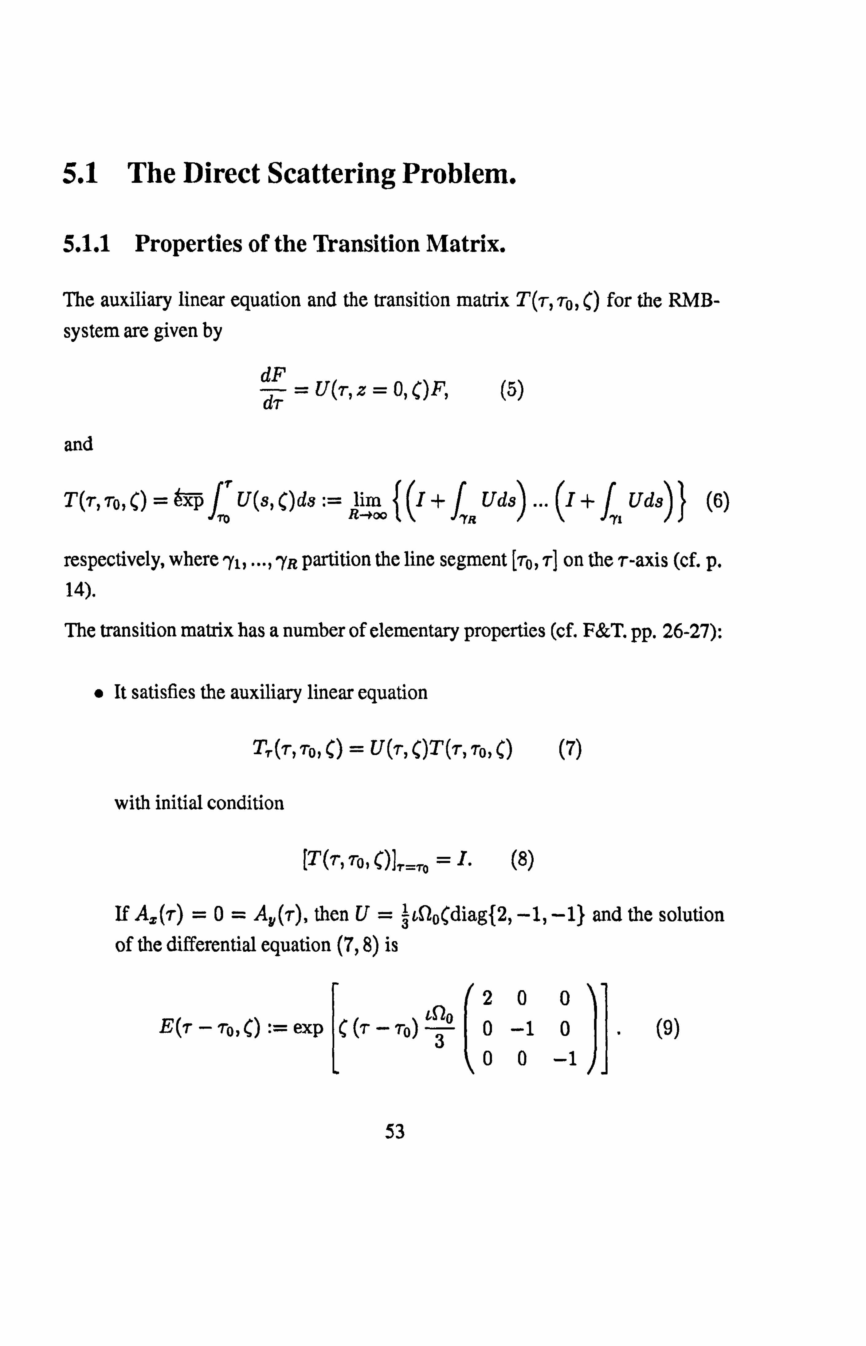
5.1 The Direct Scattering Problem.
5.1.1 Properties of the Transition Matrix.
The auxiliary linear equation and the transition matrix T (T, To, () for the RMB-
system are given by
dF dT =U(T, z=O, ()F,
and
(5)
T (T, To, tx--p Jr U(s, C) ds := lim { (I +f Uds) ...
(I +j Uds) } (6)
ro R-ºoo ? 'R 71
respectively, where yi, ..., ryR partition the line segment [To, T] on the r-axis (cf. p. 14).
The transition matrix has a number of elementary properties (cf. F&T. pp. 26-27):
" It satisfies the auxiliary linear equation
TT('r, 'ro, C) = U(r C)T (r, To, () (7)
with initial condition
[T(r, T0, ()]T=Tp = 1. l8ý
If As(T) =0= An(r), then U=3 tS'lo diag{2, -1, --1} and the solution of the differential equation (7,8) is
E(T - To, () = exP
200 To)
c3o 0 -1 0 ii" i9)
00 -1
53
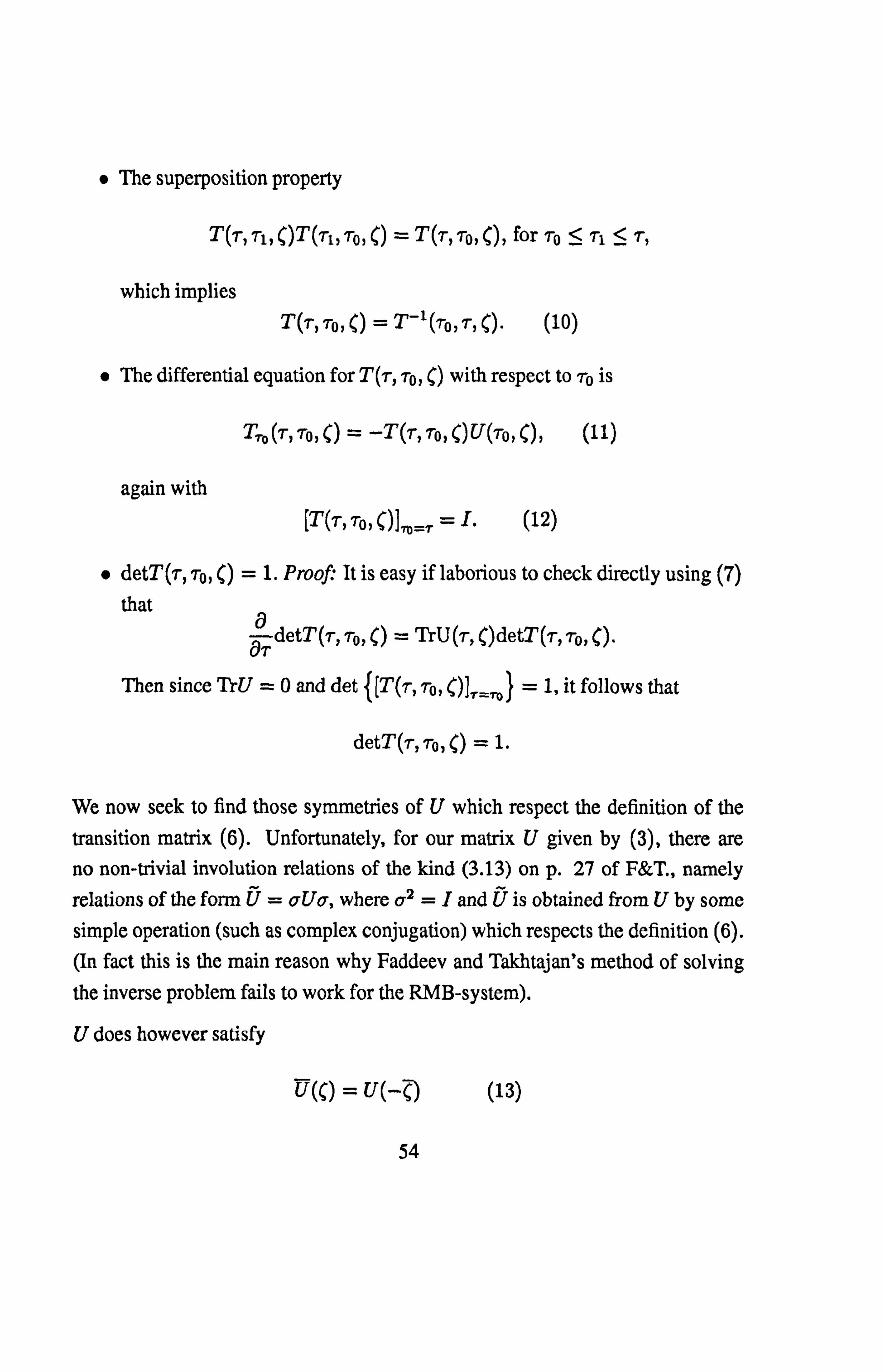
" The superposition property
T (r, r, ')T (T1, r0, )=T (r,
r0, )' for r0 < Tl < T,
which implies T (r, ro, () = T- 1(ro, r, ()
" (10)
" The differential equation for T(r, roe () with respect to ro is
TTO(r, ro, () = -T(r, ro, ()U(ro, (), (11)
again with [T(T, r0, ()}ý,
=r = I. (12)
9 detT(T, To, () = 1. Proof: It is easy if laborious to check directly using (7)
that ýTdetT(T,
To, ý) _ 'IýU(T, C)detT(T, To, ý)"
Then since TrU =0 and det { [T (T, r0, C)], f=, ro
}=1, it follows that
detT(T, Tp, () = 1.
We now seek to find those symmetries of U which respect the definition of the
transition matrix (6). Unfortunately, for our matrix U given by (3), there are no non-trivial involution relations of the kind (3.13) on p. 27 of F&T., namely
relations of the form Ü=o Uo, where Q2 =I and Ü is obtained from U by some simple operation (such as complex conjugation) which respects the definition (6).
(In fact this is the main reason why Faddeev and Takhtajan's method of solving the inverse problem fails to work for the RMB-system).
U does however satisfy
(13) U(S) = U(--()
54
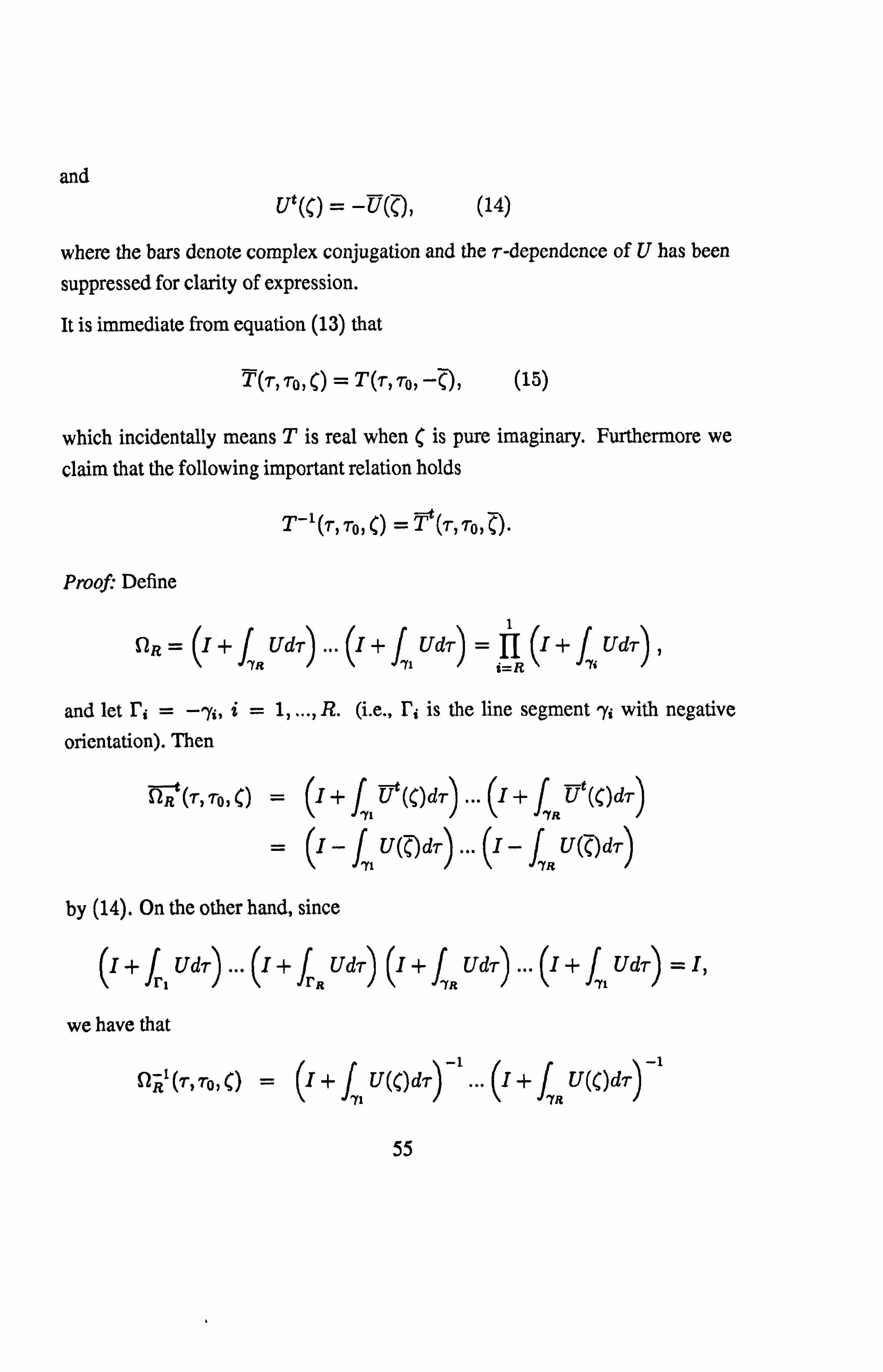
and Ut(C) = -U(), (14)
where the bars denote complex conjugation and the r-dependence of U has been
suppressed for clarity of expression.
It is immediate from equation (13) that
T (T, T0, () =T (r, 7-0, --(), (15)
which incidentally means T is real when C is pure imaginary. Furthermore we
claim that the following important relation holds
T-11T, 7-0, () -T (T, TO, -().
Proof: Define
OR = (I
+f UdT) ... (I
+f Udr) (I +f UdT) , 7s 1 {=R 7i
and let ri = -rys, i=1, ..., R. (i. e., r; is the line segment 'y with negative
orientation). Then
R (T) TOýýý - (I
+fU (C)dT) ... (I+f iJt(C)dT)
71 7R
(I -j U(CdT)... (I
-j U(ýdT) 1R
by (14). On the other hand, since
(I+judr)... (I+judr) (i+f R
UdT) ... (I +f UdT) = I,
we have that
ýRl (T, 70 ý b) - (I
+f u«)dT) -1
... (I +f U(ý)dT)
71 7R
55
i-i (I
+ frl U(C)dT) ... (I+fR U(C)dT)
(I -f1 U(C)dT) ...
(1- f U(C)dT)
R (T) TO) bI"
Therefore as R -s oo we obtain the stated identity.
Encapsulating the above using (10) and (15) gives
T(TO, T, () =T-1(T, TO, () =T (T, T0, () =Tt(T, To, -c)"
Next we introduce notation for the elements of T (T, To,
aQ ry T(T, To, b) = 77 0 E. i (T, To, C)
vPX
(is)
Since detT(T, To, () =1 and T-1(7-, To, () = Tt(T, To, -(), it is straightforward to show that the transition matrix can be written (T, To-dependence suppressed for
Equations (25 - 28) are proved by using the symmetry relations
UoE(T, () = E(T, ()F(T, C)Uo, (29)
UoF(T, C) = F(-T, C)Uo,
which together also give
E(T, ()Uo = UoF(T, C)E(T, C). (30)
Let us study the iterations of equation (22). Being a Volterra integral equation and taking into account the postulated behaviour of Ax (T), A. (z), we are assured that the Neumann series must converge absolutely. For the first iteration we write
r3 (r, ro, s) = U0 (s) +/a r2 (r, r, r-s+ r) Uo (r) dr. 11 TO
The pattern is now apparent, and so as the number of iterations tends to infinity
equations (26) and (28) result. Of course the representation (25) with 1 satisfying (27) is derived similarly using symmetry relation (29).
Lastly we remark that r and f are connected by the formulae
rR(T, T0, s) = I'R(T, r0, s)F'(2s - T- T0, (),
roR(T, T0i s) = rOR(T, T0, s), (32)
(31)
where the R and OR-parts of an arbitrary 3x3 matrix M refer to the decompo-
60
sition
M= MR + MOR I
00 M23 + m21 M33 M31
M12 M13 00 00 00
The identities (31,32) follow directly from the integral representations (25,26)
and the commutator relations
[E, T R] = 0, [F, I' R] =0= rF, I'Rj .
5.1.3 Integral Representations for the Jost Solutions.
It is first necessary to introduce some notation. Let Ll (R) be the vector space of absolutely integrable, measurable functions on R with the standard norm, and suppose L3x3(R) is the normed space of 3x3 matrix functions M such that Mij E L' (R), i, j=1,2,3, with norm
IIMII :=JL IMi1I (s)ds < oo. °O i, j=1,2,3
Now the Jost solution matrices are defined to be the limits
T± (r, () _ slim o
{T (r, ro, () E(ro, () },
for SER, (cf. P. 15). The proof that these limits exist providing Ax (r), Ay (r) E LI(R) exactly parallels the existence proof for the 2x2 solutions T± (x, A) in F&T. pp. 39-40, and we choose to omit it here.
and for each fixed r, I'+(T, s) E L3x3(T, oo). On the other hand it is immediate
62
from equation (16) and the definitions of Tf (T, () that
T-1 (r, ý) = T: 'L _ (r, -()
(= f (r, (), when E R) . (36)
Hence
T+(T, () "= lim {T (T, 7o, ()E(TO, ()}
TO ++00
_ [I
+1 00 f+ (r, s)F(T -- s, ()dsJ E(T, (). (37)
T
Notice TT satisfy the auxiliary differential equation
dTf_ dT II (T, ( )Tt I
With
Tf(7, () = E(T, () + o(1), as r -+foo.
5.1.4 The Reduced Monodromy Matrix T (C).
For( E R,
T(() := , r-*+oo,
limes-oo {E(-T, C)T(T, To, ()E(To, (38)
and so by (16) it follows that
T'1 (C) = Tt(--C) (= T (C) when (E R) . (39)
Furthermore since detT(T, To, C) = 1, we also have
detTT(T, C) =1= detT(C). (40)
63
Therefore we conclude that the Jost solution matrices and the reduced monodromy
matrix are unitary with determinant 1. They are defined for CER, but their
columns and coefficients respectively may be extended into either the upper half (-plane II+, or the lower half (-plane II-, according to the fundamental integral
representations (33,37) of T± (-r, ('). In fact, writing
we deduce from (33,37) that the columns T+1) (T, (), T! 2 (T, (), T! 3) (r, () extend
analytically into II+, whereas Ti1) (r, (), T+2) (T, (), T+31 (r, () extend analytically into H. Moreover, because r_ (r, s), r+ (T, s) are absolutely integrable functions
of s for each fixed T, the Riemann-Lebesgue Lemma implies for Im( > 0,1(1 -3 00,
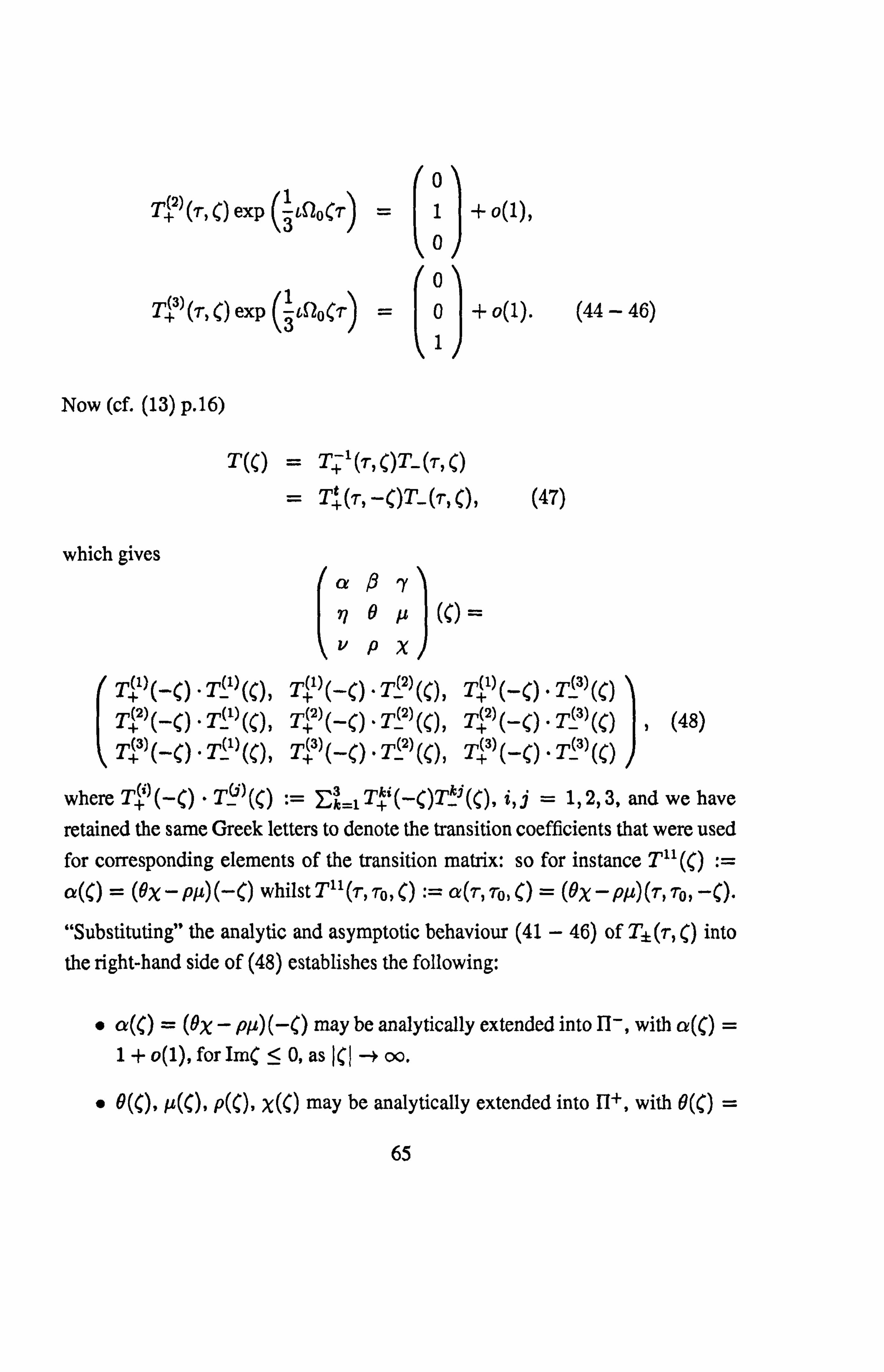
T+3) (- C) " Till (C), T+ (-C) "T2 (C), T+31(-C) "T ý3) (ý)
where T+'1(-() " TYl (S) := Ek_1 T+i(--()Tk'((), i, j=1,2,3, and we have
retained the same Greek letters to denote the transition coefficients that were used for corresponding elements of the transition matrix: so for instance T" (()
with &(s) E L'(0, oo), after a trivial rescaling of the integration variable s. Simi- larly if we substitute (55) into (53), change the order of integration in the double integral, and let L -+ oo, then we find
77(() = fC {A(s)
+ J-. lI'+ (s, s- r)Aý(s)+
+ (s, s- r)Ay(s)] e-`00s''dr}
which may be written
ooq(s)e'c°ds'
with ý(s) E L' (R), after rescaling s.
5.1.6 Temporal Evolution of the Transition Coefficients.
The evolution equation for the transition matrix is given by (cf. F&T. pp. 28-29)
i. e., Tz(r, ro, () = V(r, ()T (r, ro, () - T(r, ro, C)V (ro, (), (56)
suppressing the z argument.
We know that T±(T, () : =1imTO, f... {T(r, ro, ()E(ro, ()}, and also (cf. p. 41)
lim {V (T, z, () }= -r--rfoo
2cKLdiag {2, -1, -1} , 3 (C2 - 1)
where R -3 K= N2hö > 0. Therefore, if we multiply (56) on the right by E(ro, (), then examination of the limit
roh } {T. (T, TO, ()E(To, ()} _
ýli} {V (, r, ()ý'(T, To, ()rrE(To, ()-
T(T, TO, ()V(TO, ()E(To, b)}
obviously leads to
özT}ýT'ý) =V (T, ()7'f(T, C)- 3C1)ý'f(T,
C)
In a similar way, bearing in mind
200 0 -1 0 (57)
00 -1
T (() := z-º+
limý_ý {E(-T, C)T \To Too ()E(To, ý)} ý
we obtain
200 T: (C) =3 ((a
- 1)
I\0 -1 0I T(C) I" (58)
001I
As we shall see, the differential equations (57), (58) completely determine re- markably simple temporal evolution of the scattering data for our RMB-system.
From equation (58) it is clear that the transition coefficients 9, it, p, X and a are
2tK(
69
all independent of z:
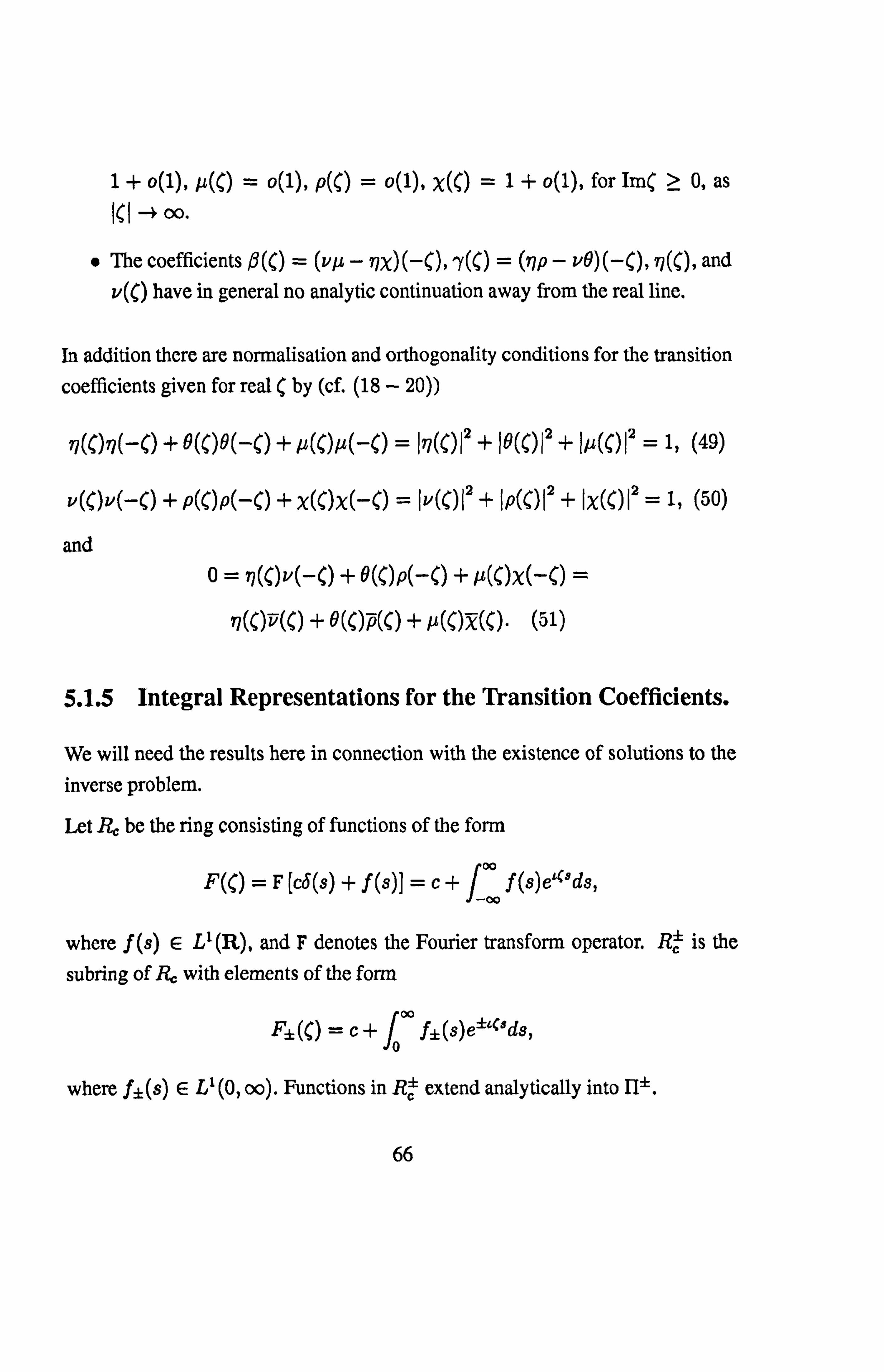
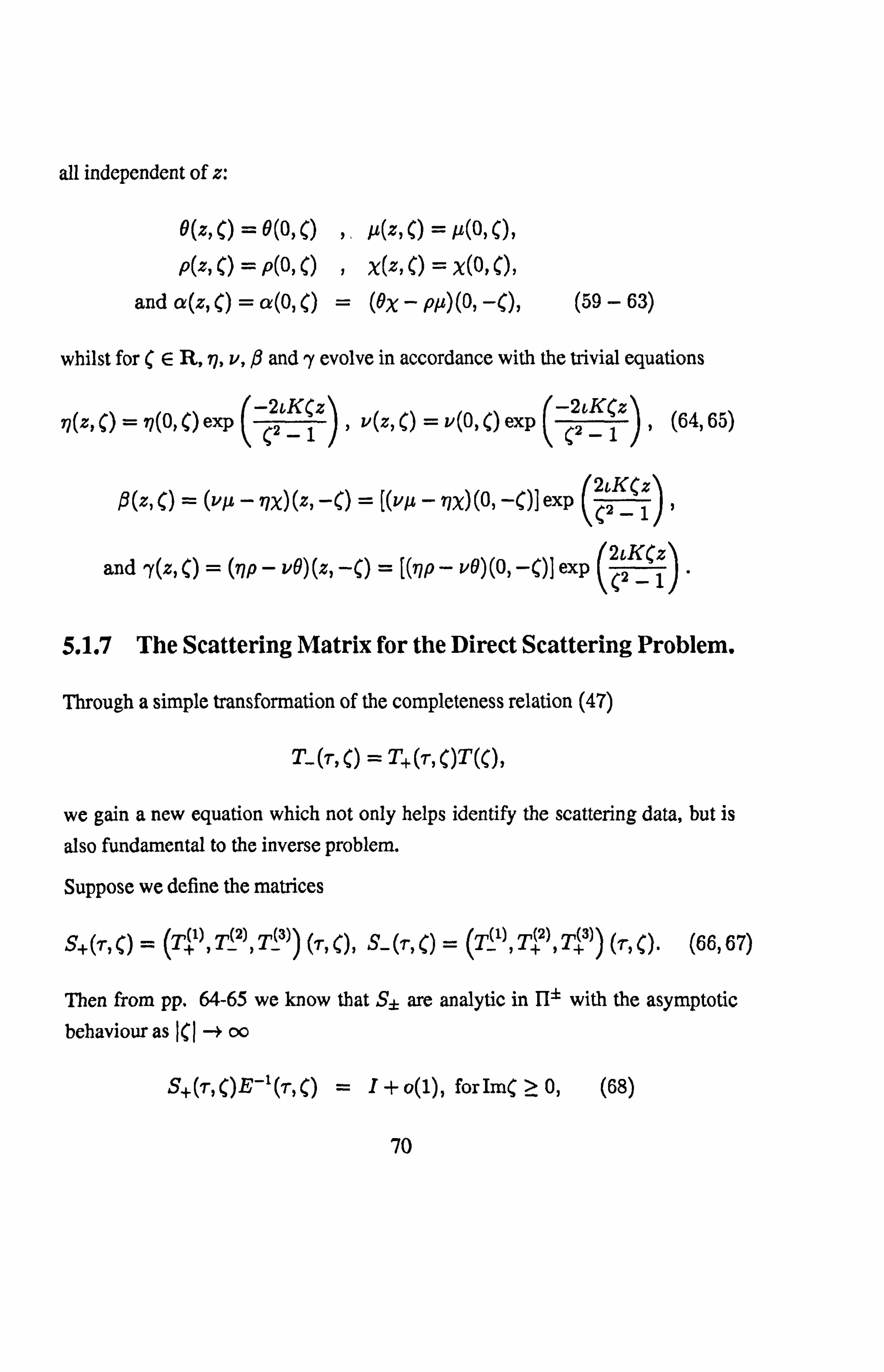
e(z, C) = 0A C) ,. µ(z, C) = µ(o, P(z, C) = P(o, C) , X(z, C) = X(Q, C),
and a(z, () = a(6, () _ (eX - Pp) (O, -(), (59-63)
whilst for (ER, rl, v, 0 and y evolve in accordance with the trivial equations
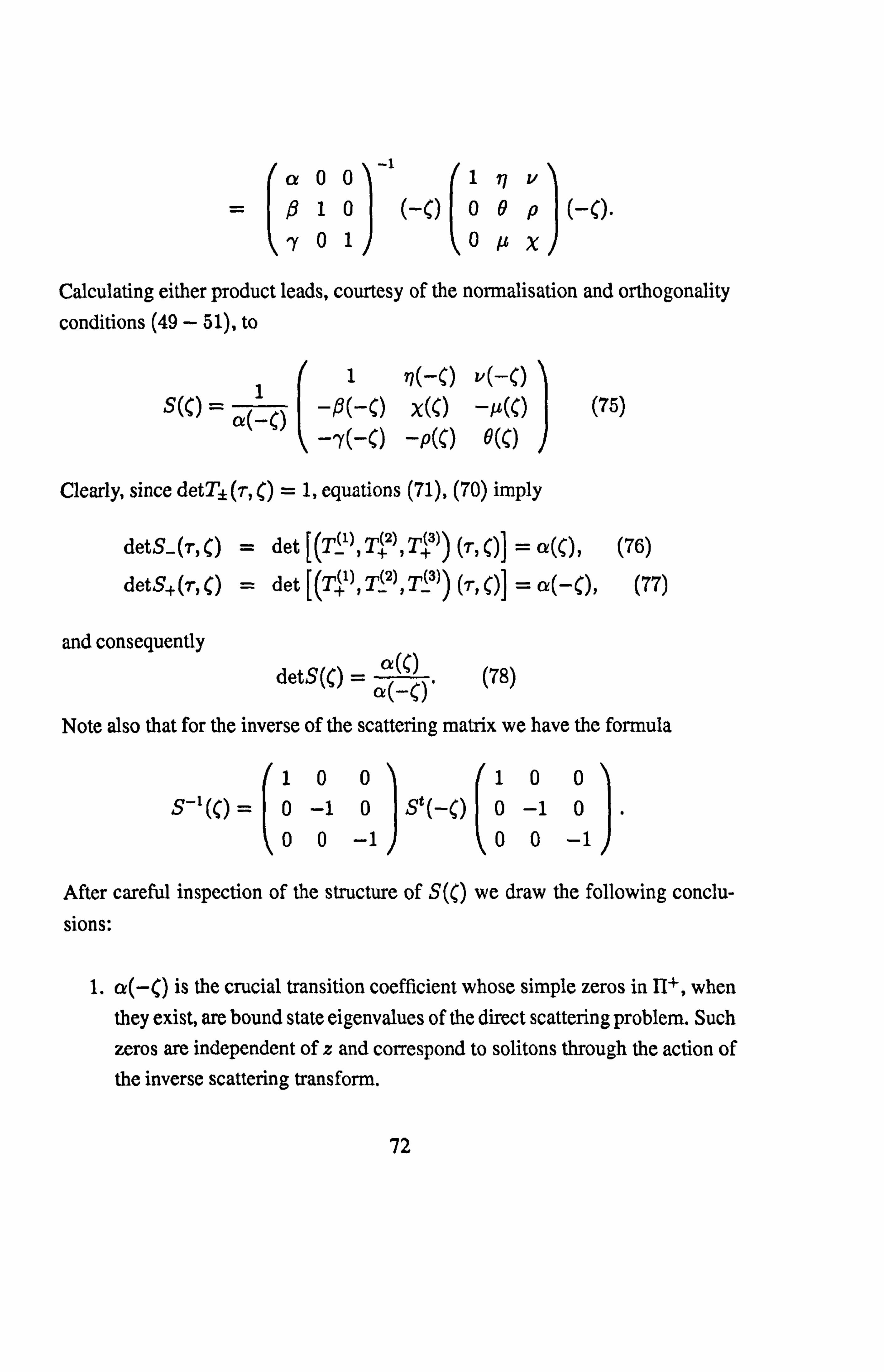
Note also that for the inverse of the scattering matrix we have the formula
100100 S-1(0 =0 -1 0 St(-o 0 -1 0.
00 -1 00 -1
After careful inspection of the structure of S(() we draw the following conclu- sions:
1. a(-() is the crucial transition coefficient whose simple zeros in II+, when they exist, are bound state eigenvalues of the direct scattering problem. Such
zeros are independent of z and correspond to solitons through the action of the inverse scattering transform.
72
2. The functions and are reflection coefficients for the direct scat- tering problem. Pure soliton solutions are obtained by setting
77(-() =0= v(-C)
as will be seen later.
5.1.8 Transition Coefficients for the Discrete Spectrum.
In order to make the analysis more straightforward we assume that the zeros of a(-C) in n+ are simple and do not occur on the real line. Since a(-() = 1+o(1),
as I() -- oo, for Im( >0 (cf. p. 65), there can be no cluster points of zeros in 11+, and so a(-() must have only a finite number of zeros.
If a(-() does possess zeros, then it is trivial to prove they occur either in pairs symmetric about the imaginary axis, or as single pure imaginary zeros. Indeed
we know T(-() = T(j, which means that if a(-(, ) = 0, then also a(Ca = 0,
where (a E n+ is some zero of a(-().
Evidently a(-() = (9X - pp)(C) may have zeros at points where for instance
zeros of 9(C), p(C), or 9(C), p(g), or X(S), p((), or X(O), p(() coincide, as well as zeros at points for which none of 9(C), X(O), p(g), p(() are zero.
Let the set of zeros of a(-() be given by
Z (a (-ý)ý _f (r+ E II+I r=1,..., n= (nl + 2n2) (a) 9, X7P)µ) 1)
where nl is the number of pure imaginary zeros, and n2 is the number of symmet- ric pairs of zeros. Then
Z[a (()] ={(,: E 11- 1r=1,... n(a, 9, X, p, µ) }ý
where (,: = -(, +, for each r.
73
Now evaluating equation (77) at (_ (r , and equation (76) at gives respectively
det (T+1>> Tý2)> TI3» (T, C. +) = 0,
= 0. and det (T ý1), T(+2), T(3» (T, (r -)
Hence there exist 2n coefficients C j) p? (z), j=1,2, r=1, ..., n such that
T +1) p rT (2) (r,
b*) +p *T (3) (r, (*) (79)
and also 2n coefficients C E) pir (z), j=1,2, r=1, ..., n such that
(These choices are consistent with later theory in Section 5.2, cf. p. 89).
In conclusion, the 2n functions p (z), j=1,2, r=1, ... m, will be called the
transition coefficients for the discrete spectrum, they are part of the scattering data which characterises the auxiliary linear problem. Observe that if c, + is pure
75
imaginary, then pl , pr are real, and if (, +, (; are a symmetric pair, then
pä=pi) p8-Pr)
as can easily be checked using (79) and the relation Tf(ý) = T±(-j. The coef- ficients p,,, (z) are dependent on pj (z) through equations (84 - 87).
5.1.9 Trace Formulae.
The results of this section allow us to minimise the number of parameters com-
prising the scattering data, and will also be needed in Chapter 6.
Let the set of zeros of a((), 9(C), and x(() be written respectively as
Z[aic)1 = {-cýaj'Rýýa, >0, j =1,..., ni}
U{ -bak , Ca E II- Ik=
nl -I- 1, ..., nl +n2 },
{ c(e, jR/D(B, > 0, l=1, . ., n1B} U{
(9,
n, -SBm E n+I m= nie + 1, ..., nie + nae} ,
=1 c(xp IR 3(xn > 0, p=1, ..., nlx )
+ l1 ýxaý -Sxa E II g= nix -i-1, ..., nix -}- n2x
Then we claim that for (E n-,
exp t 00 10,; [1- (in(s)12 + Iv(s)12)] --
ds x I
2ýr
roo rsr rr fl((+ nj n2 (b + b)
(- )'
(88)
/ /ý -1 b- Lýa
l_
ý k-nt+1 (b/ý
. +. bak) (C Cal. )
76
whilst for CE II+,
exp -6 log [l -
(1(8)12 + Ill(s)12)] ds 9(ý) = 2joo oo s ri ý-6/(81 nlo+n2e (C-e9m)(C+C6m)'
(89)
(1=11 C+ ýi8ý
m=jnil, e+1 (C
- CBm ) (C + Cem )
b %oo log [1 - l1v(s)I2 + Ip(s)I211
X(ý) = exp - 2ý J_ao 8-( JJ ds x
nL nlXý'X (C - (Xv) + TXv)
11 ý ýX
11 r
P=1 C+ L(XP
g=niX+1 (b
- CXv) (C + CXv) . (90)
Formulae (88 - 90) can be proved by the same method used in F&T. pp. 50-51
for deriving the "trace formula" in the 2x2 case (following Ablowitz et al. [33],
equations (94,95) below will be referred to as trace formulae ). However, for
completeness we prove the most important relation (88):
We know that a(() = (OX - pµ)(-() is analytic in 11 and for ER we have
the normalisation condition
ia(C)I2 =1- (I77(()12 + IV(C)12 )"
Introduce the modified function
z)
rCIO (91) a(() "= CY(() H
(_ 6("j nlH (/b +
. 'I=1 (+ 6"ai k=1nii+1
(b +C ah)
(b - bah)
Then for CE II', ä(() is analytic, has no zeros, and ä(() = 1+o(1) as oo. Furthermore, the function logä(() is analytic for Im( < 0, continuous up to the
real line (since a(() is assumed to have no zeros when (E R), and log&(() -> 0
as I(I -+ oo"
77
Suppose we define
f (s) = log ä(s)
ER s-C 'Cý
and integrate f around the contour y shown below:
Ims
We have that
) I (fr(O,
R)
ff (s)da - (( , e)
- �[-R, C-e]
f
C+a, R] f (sds,
where I'(0, R) denotes the semicircular arc centred at 0, radius R, and r((, e) is
since Re {log&(s)} = log 1&(s) I= log ha(s)1. Equation (88) follows directly from (91) and (93).
Finally, if we take logarithms of (88,89), and expand the denominator of the in-
tegrands using the binomial theorem together with the fact that Ir7(s)l2, Iv(s)I2,
ßµ(s) 12 are even functions, then we obtain
loga(c)
log8(S)
00 00 2)] s2t -2ds Iv(s) 1 ýý (2, {-
2ýr j_iog [1
- (1ý(s) 12 +
2t nl 2r-1 ni+n2 r + (bati 1- Zak 2r-1)
, (94) (2r - 1) _1 k-nl+i
\
00 00 {- 2ýr oo
log [ -ý E 2r-1 J- 1 ý r=1
+ Iµ(3)I2/J 32r-2d3
nie nie+nag _
- 2t
(, CB)2r-1 E
C. �+ 1 2r_1 )
(2r - 1) +(- Cem 95 ! =1 m=nlg+1
There is obviously an analagous expression for logX(C).
79
5.1.10 Statement of the Scattering Data.
The discrete spectrum scattering data is completely determined by the following
sets of parameters:
{ý«, ERI j=1,... ýnl}U{C«k, ý«k(k =n1+1,.., nl+n2I
and
ER {PL>>P2+j j=1, ..., nil Ul pitý, pi%, p2Ik, ý2k) k= nl + 1, ..., nl + n21 ,
where pik, pak are the transition coefficients for the discrete spectrum associated to bltk, and p ,, ppk are the coefficients associated to -yak
The continuous spectrum scattering data is given, for (ER, by
{77(o, (), V, (), v(o, (), v(o, (), µ(o, (), TO, (), P(o, (), P(o, ()} , plus either
or alternatively
where
1 B(o, a 8(0, (), x(o, o, X(o, C)} ) l
CBt , bB.,
(Bm )
(Xr l bXQ )
zXQ J1
1=1, ..., nie, m= nie + 1, ..., nie + nae,
p=1, ..., nix, q= nix + 1, ..., nix + n2x,
in view of relations (89,90).
We already know the z-dependence of the transition coefficients for the discrete
spectrum and of i and v: see equations (81) and (64,65). The remaining data are constants of the motion.
80
5.2 The Inverse Scattering Problem.
5.2.1 Derivation of the Riemann-Hilbert Problem for the RMB- System.
Our starting point is the defining equation (74) of the scattering matrix S(():
(T(1), T+2), T+3)) (T, () _
(T+1), T j2), T(3)) (r, b)S(()
(96)
Suppose we normalise the Jost solution matrices by defining
M(T, () = T_ (T, ()E-1(T, (),
Then (cf. p. 64) the columns NM (r, (), M(2) (r, (), M(3) (T) () are analytic in rl+, whilst MM (r, (), N(2) (T, (), N(3) (r, () are analytic in II-, and directly from
equations (41 - 46) we have for each fixed T the asymptotic behaviour:
Equation (97) can be rearranged to give an expression for N(1) T. If we substitute this expression into (98) and (99) and apply the normalisation and orthogonality
(100,101) Rewriting the system of equations (97,100,101) in vector notation gives
N(l) = MM + e''n°C'
M(2) M(3) p (102) -)
(
a- a- ' a- 7'
(? i. (2) 9 N(3)
= e''noCT M(1) (77-)
v-) + (M(2), M(3» 1 0- P' (103)
aaaaµ X-
where for clarity we have suppressed the arguments, and for example a- denotes
a(-(). Lastly, multiplying equation (103) on the right by X 0_ yields
-- )
N(2)N(3)a 'a)
X
_/1. _p=
-e`ýOýT M(1)
(p 'Y) + ýM(2) , M(3)) .
(104) e- «
The system of equations (102,104) may be recast as a vector Riemann-Hilbert
problem having the characteristic matrix form (cf. equations (3.1.19), p. 108, A&C. )
m+(T, () - m_ (T, () = m_ (T, ()V (T, (), (105)
on the contour Im( = 0, where
m+(7-, (): = N(1, ý
a(-ýýo
b), M(Z) (T, (), M(3) (T, ()) $
83
m- (, r, r) := (M(1)
(T, ()' X(-() N(2) (T, ()
- µ(-() N(3)(7-, (), a(() a(() 8(-()
N(3) (T, () - P(-() N(2) (T, ()
a(() a(()
1-a(S)a(-() iS2o(rý iSZo(T7. ý e
a(() a(()a(-() 'e a((),
e-'s2o(r ý( ()
,00 a(-()
e-ýs2o(r ý00 a(-() ý
and m±(-r, () -+ I, as ICI -+ oo.
For future reference we note
I
m_V = m+ - M-
= (e_40(T LM(2)
+ 'Y M(3) ý e&no[T M(1) , e`noCT ry
M(1) . (106)
[a-
a- aa
5.2.2 Formal Solutions to the Inverse Problem.
Let us first deal with the case when a has no zeros. Having already established the Riemann-Hilbert problem, we may proceed just as in Chapter 2, Section 1.4.
It is necessary to find the asymptotic behaviour of m_ (r, () for large 1(1. We know from equations (33) and (37) on pp. 62-63 that
T
M(-r, () =I+ 100 I'_ (T, s) F(r - s, () ds,
N(T, () = I+1ýr+(r, s)F(r-s, ()ds, T
100
where F(r, () = exp -tSZoCr 0 -1 0 Looking for instance at col- 00 -1
84
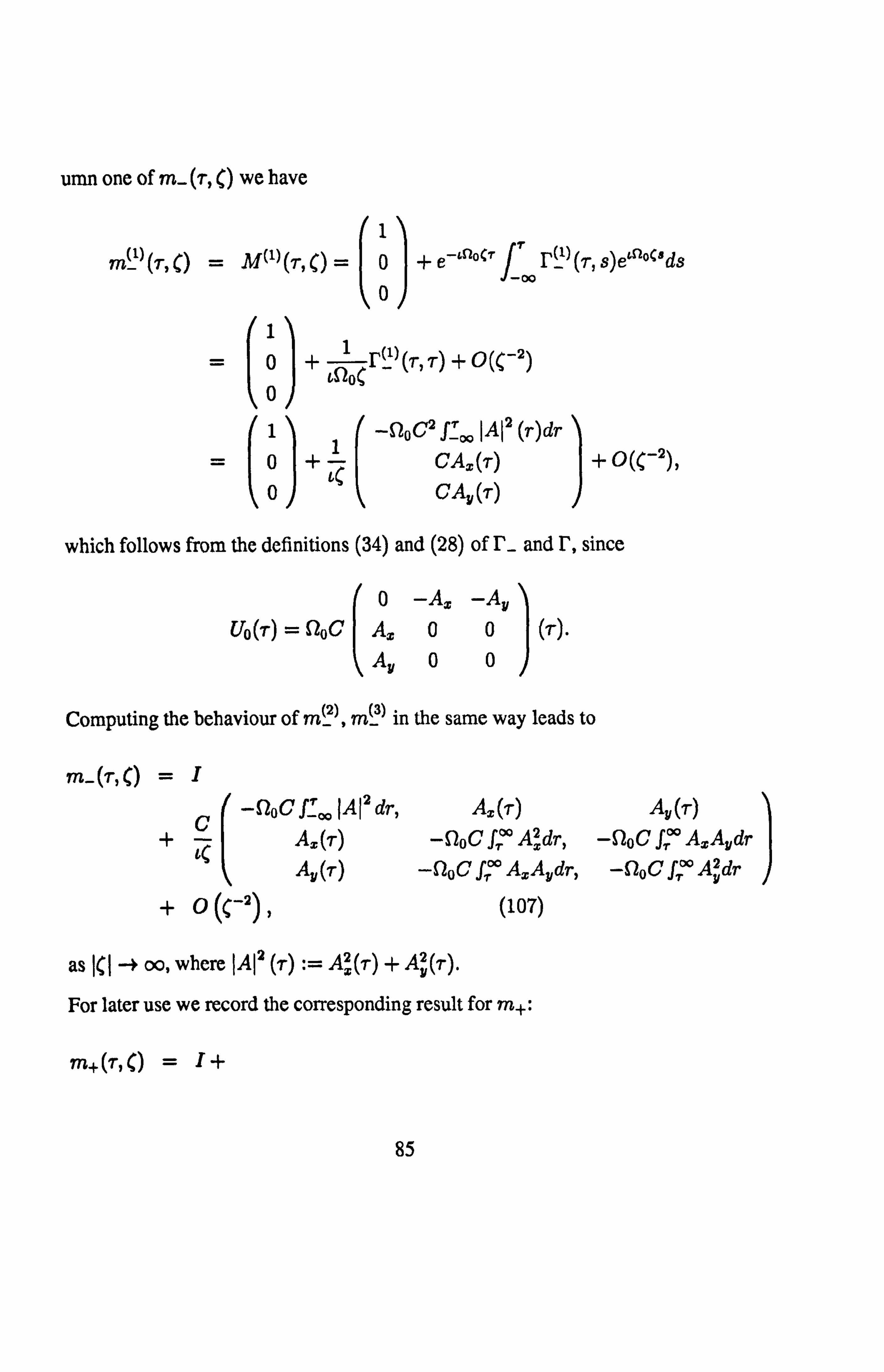
umn one of m_ (r, () we have
7rtý1ý (T, ýý _ I 1
o0 r(T, s)eoSeds MM (Tý ý) =0+- e-i'oST
J
0
I1 0 cýorrl)(T,
T) + 0(ý-2)
0b 11JA+C
CA., (r)
0 CAy (T)
which follows from the definitions (34) and (28) of r_ and I', since
0 -A-. -Ay Uo(-r) = S2oC Aý 00 (T).
Ay 00
Computing the behaviour of mý2ý, m3ý in the same way leads to
m- (T, C) =I
-f2oC fTý IA12 dr, Ax(T) Ay(r) +
cC A. (r) -f2oC f 0° A2dr, -1loC f °° AxAydr Ay(r) -f2oC f'°AxAydr, -f2oC f, °Aydr
+O (107)
as ICI --ý oo, where IAI2 (r) : =A 2(r) + Ay(r).
For later use we record the corresponding result for m+:
M+(T, C) = I+
0
85
)
r. +71 Ax(T) SZoC f. Axdr S2oC f Tý AxAydr
Lk,
Ay(r) SZoC fT. AýAydr SZoC fT,,. A? dr +o (S-2)
, (108)
as I(l -+ oo.
On the other hand, applying the projection operator P- (cf. equation (20), p. 20)
to equation (105) we find
P--I- [m_ (7, () -I) - m_ (T, ()V (T, ()} =0
() -+1 f°° m_ (T, u)V (i, u)
m_ (T 2I °° u-((-c0)
du.
Hence, for large ICI, using equation (106) gives
/ý 1 00
m a(-(:
M(2)(r, U) )+ a(-u)
M(3)(7, u) -(T, b) =- 2ýz
j (e_mnot'
SZoC f, ' JA1a dr, A.,; (-r) Ay(T) A,, r) SZoC f.. Axdr SZoC f Tý A, Aydr Av(r) SZoC fT. AýAydr SZoC fT,,. A? dr
e40 ur ä(ü) M(1) (T
o, ý) , eastowr ä(ü) M(1)(T, u) j du +O (ý-2). (109)
Now suppose that given V (r, z, () we have solved the inverse problem defined
by equation (105), obtaining mf(T, z, (). Then comparing (107) and (109) we deduce in particular that
Ay (T, z)
Ay (T, z)
_1 j°°
Mll (, r z u)du oo a(0, u) '''
00 J
eiSZour'Y(z'u Mll (T, z, u)du. 21rC -0o a(0, u)
Secondly, let us study the case when a(-C) has a set of simple zeros
Z [a(-C)l ={ (* E n+I r=1, . ., n= nl + 2n2} .
86
Consider equation (102): we have that N(1) T'ý is meromorphic in n+ with n simple poles. If we choose to set
NýL/ý ýTrý C) = N+\/. rý
ArýT+
al-r) r=1 C Cr
where the column vector N+(T, () is analytic in II+, then (102) reads
as I(I -> oo. Thus, equating coefficients of (', and assuming once again that
given V(r, z, () we have solved the inverse problem for m±(r, z, (), we obtain the formal solution
n 'ýos* *
_rr+
ýý fýz)Mza(T' z'r* ) +ý f/z)M2s(T, z, ý, ý), -
A=(T, z) =-cEe c'(0 Sr)
lbll
88
joo ý oß(z, -u) (T 1e 21rC oo a(0, -u)
m2, , z, u)+
-f (Z, -u) M23 (T, z, u) du, a(0, -u
with a corresponding expression for A,, (T, z). However, this is just one represen- tation of the formal solution. In order to acquire the other we choose to write the
system of equations (104) as follows
Ný (Tý C) +ý ýr (T)
_- X(-0
jV(2) (T, () + Pa(() )
N(3) (T ,
a(c) r=1ý-ýr
_ ed'osr a(c)
M(1) (T, C) - M(2) (, r, C), (114)
Ny cTý C) +ý CrcT) f=1C-Cr
P(-C) N(z) (T, () _ 9(-C)
N(3) ('r, ()
e`ýýsT a(C)
M(1) (Tý r) - M(3) rTý ý)ý (115)
where Nj (r, () and Ný (r, () are column vectors analytic in II-. Matching
residues at poles in the first equation, bearing in mind relation (112), gives
__ r+ rr ý oC-rT +
rr Br(Tý a ýbr ý [ý1rN(2) (T, C-) -ý iý2rN(3)
for each r=1,.., n. Furthermore, recalling the definition of the operator P+ from (20) p. 20, we have
P+ Ni +E Br(T)
+ M(2) - [m_V](2) =0 r=1 (T
=: > M(2) - 1(2) +ýB, (7-)
- P+ 1[m_V ](2)} = 0. T=1
(- cT
89
Hence
M(2) (T, C) = J(2) +1 ..
[00 [m V /(2),
(T , u) du - G7T6 J-oo u- ýý -t- bU)
n e&noCr 'rp1T 1 E
-CT )a'ýC* )M( )ýT, Sr )
r=l (C (116)
our ßu M1(T u)du - = I(2) -1
f°° e 27rc( oo a(u) '
1ý e&sksr T Pir M(1) (Tý ýr )+0 (C-2), (117)
as ICI -+ oo. By a parallel argument applied to equation (115) we also find
M(3) (r, C) I(3) +1 oo [mV ](3) (T' u) du - 2irc Joo u- (C + to)
n eri2oCr T P2r ý (C - (* ) a, ((r ) M(1) (Tý ýr ) (118)
as ICI -+ 00. Therefore, comparing asymptotic expansions for M(2) and M(3)
given by (117), (119), and columns two and three of equation (108), results in the
second formal solution
A. (T, x) _L [n'` eiS2oCr T Pr (z)
Mll (T' z' r=1
ý-) - CLý a'(O, (T) r
ýC _ eLsýouT
ý(Z, ü) Mii (T, z, zý)du, (120) ,
ý enoSrT
i2+r (z) Mll (T, z, br
)_ Ay (T, z) =_L. i C r-l a'(0, (i) b
1 %ý e&n0"T
ý z, u Mll (7, z, u)du. (121) 2ýC J_ . a(0, u)
90
5.2.3 Soliton Solutions of the RMB-System.
If the transition coefficients 17((), v(() are zero when (is real, then the Riemann-
Hilbert problem (105) may be solved in closed form. Indeed setting 77(() =0= v((), for (ER, so that the reflection coefficients ij/a, v/a, ß/a and 7/a are
zero as well, clearly causes the integral terms to vanish in each of the equations (113) and (116 - 121). Specifically from (113), (116) and (118) we have
M11(T, C)
M12(T, o
M13 (T, C)
L
n e-toCrr /ý (+ 12 +) ++M
r=l ý2r13 =1-ý
-ýf ý1rM \Tý br lTý br
ýý a'(
n -iS2oc; r e ý__�, - a'(-()(br
-r M. ýý. -sT i=1
S 'f' ýaýýla ý,
n e-is2ps. r
-8=1aý(-bä }(ý'ýýä }P °Mll(T, -(s ). (122-124)
Reintroducing the z-dependence, it follows that for s=1, ..., n
Mil (T, x, -Cs) = n e-iStoSr *
X (125) 1-E-. 11 l4-%//'4- 1 . 1-4-A r=1 'x l-, W 1 \Sr T Sa' 1
n e-ýsýC+T p(z) E
; )P e(z)MiiýTý z, _ýa ) L&-x(T -+' (. +))P+
ý++` /
e-iStorý, +r
/T r +iý2rýz) Lý ýl-ýä )ýbr
'i' ýs )p2a(x)Mii l, z, -ba )"
This is a system of linear algebraic equations for Mll (r, z, s=1, ..., n,
which in conjunction with equations (120,121) evaluated when 77 =0=v, CE
R, i. e.,
As (T, z)
Ay (T, z)
_ý Ee-&S2oCrTä (r((I+)
M11(Trxr -()' (126) r =l
_Ci' Ee-inoC: r 1ý2 (z) M11(T>x> -(r+)l (127)
r_1 a'(-(r )
91
allow us to calculate pure n-soliton solutions of our RMB-system.
Consider for example the special case n=1. We know (cf. Section 5.1.8) there must just be one pure imaginary zero of a(-() at (=t (say), R E) C>0, with associated transition coefficients for the discrete spectrum denoted by pl+(z), p2+(z) E It. To obtain real potentials A., (r, z), A,, (T, z), we assume that the reflection coefficients ß/a and y/a take the form
_ NO
- «(()
«(() - i Lný+ Im C<0 I
0, ýER, &z Im( <0. a' -if)«+iZ) ý
Observe this means the reflection coefficients are real when C is pure imaginary,
and in addition the residues of (A) (f() and (ä) (±() at ýaC are given by
Res P(C)
"t tPi+
a(() ;- a' (-cc)
Res _(-().
cc 1Pi+
a(-()' a'(-tC) 'Y(();
__ LP_+ Res
a(C) a'(-cc)
Res 7(-() " IC tP2+
a(-O a'(-tC)
Matching residues once again in equations (110), (114,115) we now find
cenofT Mll (Tý ý) = 1- a, LO (C - cý)
[P1+ M12 (, T) IC) + P2+M13
cenoFý M12ýTýý) ý aº(-cý)iC+ fý)Pl+MiiýT, -cý)ý
M13 1T, jý = W� 1ýi+M11(T,
a$ ý-cý)ýý + cý)
Ge"OP*
92
and so -1
M11(T, -cý) _1+ 2+ +P2+)
e2flo£T 4ý2a'2 (-cý)
Hence
A,,, (r, z)
Pi+(0) eXP [92oe (, r - To(z))]
1.. {_ rP'4ý(ä)±P2ý) )1
exp [290e (T - To(z))]
_Z Pi+(0)
sech [SZoe (T - Tl - Tp(z))ý , (128)
C Pi+(0) +Pä+(ý)
enofT t Cal (-6t) 20oCr
where we have used the fact that pl+(z) = pi+(0) exp (-- ), and f +1
Wz _1 ro(z) :=
ý0(42 + 1)' T1 . In
Similarly,
Pi+ýý) + Pä+ýO)
A, (, r, z) =C2 +0) a
sech 190Z (r - Ti - 70 (41 "
(129) ? i+(0) + ? a+(0)
Solutions (128) and (129) are precisely the same linearly polarised 1-solitons found in Chapter 4 (cf. equation (4), p. 40).
5.2.4 Existence and Uniqueness of Solutions to the Inverse Prob- lem.
General questions regarding existence and uniqueness of solutions to the Riemann- Hilbert problem (105) are difficult to answer categorically. However, by carrying
Pi+(z) Ca'(-ct)
93
out a simple calculation based on theory established by Gohberg and Krein (1958) [37], we can at least demonstrate existence and uniqueness in the generic sense.
First recall equation (74) for the scattering matrix S(C)
Considering that in Section 5.2.1 we also derived (105) from (74), we there- fore see the equivalence of our Riemann-Hilbert problem to the matrix factori-
sation problem on Im( =0 associated with (132). Namely, given G(r, z, (), find G± (T, z, () such that
G+ (r, z, ()G_(-r, z, () = G(T, z, (),
for (ER, where G± may be analytically extended into II}.
94
Now let R3x3 be the ring whose elements are 3x3 matrix functions of the form
F(() = cl +J 00 f (s)els°ds, 00
where f (s) E L3x3(R), and let R3 3 be the subring of R3x3 having representative
elements (s)e}C'ds, Ff (() = cI + j°° ff
where f±(S) E L3x3(0, oo). Then Gohberg and Krein proved the theorem below (cf. A&C., p. 449):
Theorem.
1. Every non-singular matrix G(() E R3x3 possesses the factorisation
G(C) = G+(()o(C)G-((),
where Gf E R31,3, detG±(() 94 0 for tEr Il, and
ýýC)=diag ýc) "' C-c "' S-c ns {((+c 'C +c ' +cl
(/
Here rcl > r,, 2 > ßc3 are integers referred to as indices.
2. If G possesses another factorisation
then a(C) = A((), G+(C) = G+(C)A(C), d_(C) = A-'(()G-(C), for
some non-singular matrix A.
3. K= Kl + Ks +' 3= ind [detG(()], where given a function g(() defined on RI, the index of g with respect to Rl is
ind (g(()] := J- 2ýc oo dý fing(()} d{.
95
Corollary. If it is further supposed that G(() =I+ o(1) as -º oo, and
GR(() =1 [G(() + 0'(()]
is positive definite, then kl = r. a = ic3 =0 and there exists a unique factorisation
G(C) = G+(()G-(C),
where G} E R3 3, detG±(() 00 for( E III, and G±(() =I +o(1) as ICI -ý oo.
In view of Gohberg and Krein's theory, which provides the standard method for
checking existence and uniqueness of Riemann-Hilbert problems, we look again at G and Gk specified by (130 - 132):
. From Section 5.1.5 we conclude G has an integral representation
G(T, C) 00
+1 °° 0 0 0 (
Os -}- T), L(-s + T)
00 e's"ds 00
00 X(s) -µ(s) e`(°ds,
-p(s) B(s)
where J-7, i, j3, ry E Ll (R), and E L'(0, oo). Hence G(r, ý) E R3x3-
" Using the integral representations (33) and (37) for the Jost solution matri- ces it is reasonably straightforward to prove Gf (T, () E R3 3. For instance,
j=1,2,3, where VI (r, ,r- s) E Li (0, oo) as a function of s. (Appropri-
ate integral representations for rows two and three of G+ (r, () are found by
means of the Convolution Theorem for Laplace Transforms, and the equal- ity a(-C)S; ' (r, () = adj [S+ (r, ()] ).
" detG(r, () = det [a(-()S(()] = a2(-()a(() ,E0 when (ER. Whilst detG+(r, () = a2(-() and detG_(r, () = a((), so that Gf may be non- singular in their domains of analyticity.
These properties of G and G± are all much as we might expect. Unfortunately, due to the complicated form of G(r, (), the "hermitian positive definite" condi- tion apparently does not furnish a clear-cut or useful criterion for existence and uniqueness. However the situation is redeemed somewhat by the following result:
ind [detG(C)] = 1 %°° d {ln [detG(ý')j} dC TT, J-. dý'
= 21rc [In (zu«) 1 a(S)1Z)] -00 00
ý'
which is a consequence of the asymptotic behaviour ci(() =1+ o(1) as ICI --3 oo. According to another Gohberg and Krein theorem on stability of indices,
Ablowitz & Clarkson (cf. p. 450) point out that if the overall index ' is zero, then generically speaking, the indices %£1, iz, i3 vanish aswell. Existence and
uniqueness of solutions to our Riemann-Hilbert problem is therefore guaranteed in a generic sense.
97
Chapter 6
Calculation of the Conserved Densities for the RMB-System.
A striking general property of integrable partial differential equations is that they
possess an infinite hierarchy of local conservation laws. It will be seen in the case
of the RMB-equations that the conserved quantities occur as the coefficients in an asymptotic expansion for log a((), and we shall represent them as functionals of the scattering data through use of the trace formula (94) p. 79.
Let N(r, z, u(r, z)) =0 be an integrable equation. Then since we have taken z to be the evolution variable and r the transverse variable, a conservation law may be defined as an equation of the form
BJ +aTF=0,
holding for all solutions u(T, z) of N=0, where the density I and the flux F are allowed to depend upon r, z, u, u1-, u,, ..., but not us. Providing I and FT are integrable as functions of z over R, and if F -+ constant as ITi -+ oo, we then find
Id T) = 0. dz C f-'00
98
I is called a conserved density and the functional f_. Idr is a constant or invari-
ant of the motion.
Now in order to obtain the conserved densities for our RMB-system, we seek a gauge transformation which asymptotically reduces the matrix
U(r, () = -ý4 ((H- + H+ (r))
to the diagonal form °O Uº
Uº ,., ýi
where each Uý is a diagonal matrix.
It is simple enough to show that each UU is conserved. In fact, because the zero curvature compatibility condition is invariant under gauge transformations
we have
The diagonal part reads
U'= GTG-' + GUG-' (1), V'= G,. G-' + GVG-',
OZU'-8TV'+[U', VII = 0.
I part reads
azU'-ar(V')°=0, and so integrating with respect to T and using the boundary conditions yields
Therefore
as claimed.
z(rý U'dr) = 0, VC.
ý U'dT) = 0,
dz (100
Since U(r, () is a3x3 matrix, there are two stages involved in the diagonalisation
procedure. First let us reduce U to an R-type matrix U'(r, () = Z(T, () (say), by
99
applying a gauge transformation Gl (r, () = (I + W(7-, C))-1, where W is chosen to be an OR-type matrix with the asymptotic form
b) _E 0.0 ý (2)
Wn(T) W(Tº
n=
+p (ICI-00)
1 ýn
as I() -s oo. (The R and OR-parts of a3x3 matrix were defined on pp. 60-61).
Substituting into equation (1) it follows that
(I +W (r, ()) Z(r, C) = -WT(r, () - (CH + H+(r)) (I +W (r, ()) ,
which is equivalent to
ihZ = (H- + H+W, (3)
thWZ = -ihWT + H+ + (H-W, (4)
after splitting into R and OR-parts respectively. Equations (2) and (3) imply
Z(T, () = -b(H - ti 0 00 (H+Wn) (T)
+p (ICI") , (5) n
as oo, whilst eliminating Z from (3,4) gives
£? WT-H++([W, H-]+WH+W =0. (6)
0 A, Ay Next suppose we define or= diag {1, -1, -1}, and Hs(r) = Ay 00 (T).
Ay 00 Then equating coefficients of powers of ( in equation (6) and employing the for-
mulae
-QH' = Ha,
100
0W ia yy13 n>n
[Wn, H-1 = h. SZo -W, a, l 00= hS2oQWn,
-Wnl 00
0 Ax, Ay
H+ = -chSZoC -Ax 00= -ihS2oCQH', -Ay 00
(where C := eqo/h), leads to the results listed below:
0 Ay, Ay W1 = -iC A. 00
Ay 00 n-1
Wn+1 = ýn 1 ýnWnT -ý WkH+Wn-k ,n>1,
W2
iiac° X k-1 /
C0 Azr
, Ayr
_ý -AsT 00I= (-i)2C (S2°/ HT7 17 no
-AyT 00
10 Axrre Ayrr 0 Ax, Ay
Wg = tC 2 AzTr 00+ C2 JA12 Ax 00 o Ayr., 00 Ay 00
= (-6)3C (Hr + SC2H'') (0)2 S2o
W4 ý-i)4C 3
{HTM + S2öCa [(H 3) + He'H, r
+ H, r1182J J' (h-) T etc.
Clearly Wn may be written
//l n-1
1ý wnýT) = `_LInC (
\SZp) Wn(T), n>
where w. is a real symmetric OR-matrix whose elements are polynomial func-
tions of Az, A. and their r-derivatives. The power of a determines whether W�
101
is symmetric or anti-symmetric. Hence, substituting for H+ and W,, in (5), our expression for Z becomes
z= 3iSZodiag {2, -1, -1} C
00 + npCý E
n-1
Axwn2 + Aywn3 00
0 Axwn2 Axwn3 C-". (7)
0 Aywn2 Aywn3
We remark incidentally that the diagonal parts of H+ W2, ' are total derivatives with respect to r.
The second step is to asymptotically reduce Z(r, () to 0(r, (), a diagonal matrix,
using the gauge transformation G2(r, () = (I + M(r, where for large ICI
00 M(r, F M'ý(r)
+O n=1 C
and
We have
000 M�(T) =00 Mn3 (T).
0 M, 3ý2 0
(I + M)0 = -M,. + Z(I + M),
or, in terms of diagonal and off-diagonal parts,
0= ZD + ZODM, (8)
MA = -MT + ZDM + Z°D.
Eliminating 0 therefore gives
MT - Z°D + IM, ZD1 + MZODM = 0.
102
It is convenient for the moment to use equation (5) rather than (7) for Z, then matching coefficients of powers of C we obtain
000 M1T _
(H+WI)on _ -LQoC2 00A. ýAy 0 AxAy 0
(9)
Mz, = -h f (H+W2) oD+ [(H+ WJ)D, MI]J
000
_ -C' 00 AyAyr 0 AxTAy 0
+ 1 o00 fZoC' 00 (Ay
- A2, ) f loo AxAyds
0 (A. - Ay) fToo AxAvds 0
etc., and by equation (8)
0=F Al
1=-i
CH- -}. (H+W1)n
+ (H+W2)D + (H+Wi)°D Ml+
fi (2 (N+tiýs)D + (H+Wi)
(3 M2 2)OD ml
+0(1(1-4) .
As was demonstrated at the beginning of the chapter, the diagonal matrix co- efficients of this expansion for A are conserved densities of the RMB-system. However, after some rather laborious calculation, it becomes apparent that the coefficients of even powers of C are total derivatives and can be ignored.
Consider for example the coefficient A2 = (chi)-1 [(H+W2)D + (H+W1)oD Ml].
103
Plainly we have
C2 JA12 00 (H+w21ýdT= fýöT 20 Ax 0
1}dr=o. /ý
00 Av
Dealing with the second term
-h rH+wl`on Ml = -cSZoC2diag
{0, `4ý`4yMi3' Ay`ýYMi3}
is a little more complicated. From equations (19), (26) and (27) on p. 35, we find
p2,. dT = 0. d fý AxAydT oc 1,00 00
i. e., 1-00 AxAydr := rc, (say),
is also an invariant of the motion. Moreover, since equation (9) only defines
M , 23(-r, z) up to an arbitrary constant of integration, we may choose
T1
Mý(T, x) = -tS2oC, [fý (A. Ay) (s, z)ds - 2ý1
Then
f 00.0 00 OD -tfloC'A, AyMI"dr 0f
w -ý
(H+W1)M1dT.
It is also instructive to examine the coefficient 03 of (-3. Observe that
Tr { r00 A3dTJ = 0, 00
which as we shall see presently , is a condition required for consistency. Indeed
We now introduce some notation and theory regarding the monodromy matrix TL(C) = T(L, -L, (). This theory helps to finalise the form of our expansion for A, and will enable us to represent the conserved densities in terms of the scattering data established in Chapter 5.
105
Let the monodromy matrix be written
/r Q'L NL 'yL
rr TL(C) = iL 8L PL vL PL XL
where
aL(C) - (OLXL - PLµL)(-C), RL1() - (vLIAL
- ? %LXL)(-b)v
'YL(C) _ (? 7LPL - iLOL)(-()"
The elements of TL satisfy the usual normalisation and orthogonality conditions, and we know detTL(() = 1. Then the reduced monodromy matrix is given by the limit
T(C) =l im {E(-L, C)Ti(C)E(-L, C)} e fiL'no(CYL(C),
e}LLnoCNL(C)f e-siLSZoCryLIC) r Jim e-#`LnoCýL(C)r esiLnoCBL(r), esiLf2oCYL(b) "
(10) L-ºoo \b
/ e}anoCULýC)ý eIiLnoCPL(C), e3aLnoCXL(b)
Furthermore, according to equation (2.19) p. 23 of F&T., the sequence of gauge transformations G1, G2 transforms TL(() in such a way that
TL(() = (I + M(L, ()) (I +W (L, ()) x
exp [1-'L
0(r, C)dIr (I +W (L, ())-1(I + M(L, ())-1 " (11)
Since detTL(C) = 1, this relation implicitly requires
Tr JIL
ä(r, C)dr = 0, VC, and so Tr {f' Ajdr = 0, Vj.
106
We are finally in position to draw together the results of our calculation. Equations (7) and (8) imply
o(T, () = 3aflodiag{2,
-1, -1}(+
tZ2C2 00 to 1"
-"dia {A w1a +A w13 A w12 Ay w13} + p ýQJ gxnUn, x ný "
Evidently this equation describes those conserved densities which are polynomial functions of A., A, and their r -derivatives, in terms of the set of scattering vari- ables
IV(b)12vC j,
C,,,, Zawlj = 1,..., ni, k= ni +1,..., ni+nZ}.
109
Chapter 7
Perturbative Effects in Real Optical Media.
So far we have been concerned with the solution of an idealised mathematical model which ignores the various loss mechanisms and inhomogeneities actually occuring in a typical optical medium. Under these simplifying assumptions we have explicitly proved the solvability of the RMB-system by the Inverse Scattering Transform method, and studied the associated hierarchy of conserved densities. We shall now exploit the exact mathematical results of the preceding chapters to derive the following evolution equation
f00 (A2-1 -+-132,. _i) dr =
J°° 00
AL2r-2AdT, (1) dz o0
where N3r>1, A := (-A17 Ax, -Ay, Ay)t, and L is a4x4 matrix integro- dil%rential operator to be defined later. Given a system of RMB-equations suit- ably altered to model an arbitrary perturbing effect, equation (1) may be used to calculate the corresponding variation with distance z of the invariant functionals
00
1ý (A2. _1 + B2_1) d-r
110
specified in Chapter 6. The main reference for this chapter is a paper by J. N. Elgin (1993) [13] entitled "Perturbations of optical solitons". Elgin proves that a similar
equation to (1) holds for the simpler case of the Nonlinear Schrödinger equation,
which has only a2x2 auxiliary linear problem (cf. [13], equation (4), p. 4332).
7.1 Proof of the Evolution Equation for the Invari-
ant Functionals.
Let us recollect some basic theory out of Chapter 5:
9 The AKNS eigenvalue problem for our RMB-system can be written
. The Jost solution matrices T± satisfy the differential equation (2) for each z and have the asymptotic behaviour T±(r, z, () = E(r, () + 0(1), as r -4 foo. That is
Tt" ) (T, xr C) _
el'n0c* 0
0ý e-}9nacT 00
I
0 0+ o(1), (3)
e-VotT as r -º ±oo.
" T±(r, z, () are connected via the completeness relation
T_ (r, z, () = T+ (r, z, C)T(z, ()
111
Columnwise, suppressing r and z, this reads
a )(C), (4) T'ý'ý(C) = (C)T+1)(() +i1(S)T+2){() + v(()T+3 T ýý)i()
In view of the facts above, we proceed to find z-evolution equations for the tran- sition coefficients a, ß, -y, i, 0, E. c, v, p, X by employing the method of variation of parameters.
Suppose we define the column vector
Y= fs = (f1s, f2s, f3s)t E C3.
Then equation (2) implies
yT-Uy-U, f=T, (10)
where U, f = i20C (-As, fz - Ay: f3, Ax: fl, Av, fl)t. We already know that a suitable solution of the homogeneous equation (2), with the property y -ý
which follows because the matrix T+ is independent of z for large r (cf. equation (3)). Letting r -+ oo and equating our two expressions for eT' (() yields the
required evolution equations. For instance, comparing coefficients of T! 1) (C) in (12) and (13), namely
Corresponding equations for the remaining six transition coefficients are calcu- lated in the same way after choosing either f= Tý2ý (C) or f= T9) (C). In fact, ifT`j((), i, jE {1,2,3} denotes the (i, j)-th element of the reduced monodromy matrix, then we find
00 ý Tf'(C) = SZoC1
ý {Axý ýT+`(-C)7'ý'(ý)
-T+ (-C)T2'(C)ý +
(14) Av: [T+3(-()Ti'(() -7+ (-()T3'(()] } dr.
Suppose we now introduce the eight functions
a(i, j) "= T+'(-()T2j((),
b(i, 9) "= T+`(-7'i'(C),
C(i,. 7) "= T+'(_7'sj (0,
d(i, j) "= T+(-Tl'(S),
k(i, j) "= T+'('Tli (C)-T+'(-ý)T2j(C)ý
l(i, 9) "_
T+`(-()Tlj(() -T+'(-()Ts'((),
m(i,. 7) "= T+i(-()T3j(C),
n(i, j) "= T+'(-()T2j (C).
115
Then by virtue of equation (2) there is a closed system of eight first order differ-
ential equations for a(i, j), ..., n(i, j) of the form
ar = -cSZo(a + SZoCAxk - SZoCAyn,
br = aSZo{b + SZoCAxk - SZoCAym,
cr = -tSZo(c + SZoCAyl - SZoCAxm,
dr = aSZo(d + SZoCAyl - SZoCAxn,
kr = -2SZoCAx (a + b) - SZoCAy (c + d),
IT = -SZoCAx(a + b) - 2SZoCAy(c + d),
mr = SZoC (Axc + Ayb),
nr = SZoC (Axd + Aya). (15-22)
Note also that equation (14) becomes
a(i, j)
a/ /'ý b(i j)
azT f'(ý) = sipc' Jý (-iixz, A-,,, -ALx) AIIz)
C(i: j) dr
d(i, j)
_ sloC f oo A'ý(z, . 7)dT, (23)
ý
where A= (-A,,, Ax, -Ay, Ay)t and * (i, j) := (a, b, c, d)t(i, j).
Furthermore, suppose we set i=1=j. Then in particular we have
Making use of this new notation equation (1) becomes
d 00 = dz 1_00 (A>-1-f- B2r-1) dr (A, l L2r-2A)
(L2r-2A, I A), for N ar > 1, ý L2AxI L2''-4A> , when r>2. (25)
Finally, as a consistency check for our results, we compute the right-hand side of (25) in the cases r=2 and r=3 using equations (18 - 27) p. 35, anticipating both answers to be zero. Applying the definitions of L and L one finds
-A-- ý (A,,
Ax A.
-Ay ýio AyT
Ay Ay,
A_ I ,. I A__ LA =L1 --; 1= _n 1 -;. `T 1, (26) -Ay Ia co I AyT
Observe that equations (26,27) hold independently of whether the system is per- turbed or not. Hence
since
and
(AzI L2A) = (LZAI A) -
G'2NA AT 2ceoSZo
A+( A, t l A) i 0,
00 12(ATI A) a1. aT {IA} dT
(ASIA) oc Jý ö% { JAý2} dr oc J° {sp7 + ps} d7
vanish due to the boundary conditions. Moreover
CL AzI LaA/ \_ Ca Nh Ar 2cs0SZ0
because
LZA + 1A,. 1 LaA> = 0,
(ArI OA) a f00
ý Or {IAri2 + JAý4} dr.
7.2 An Application of the Evolution Equation for
the Invariant Functionals.
7.2.1 The Perturbed Model for an Absorbing Medium.
Our original RMB-system, given by equations (18 - 27) on p. 35, can be modified quite simply in order to take account of basic dissipative processes.
Recall from Chapter 3 that the dipole displacement and momentum operators are
Q- q0 (A1, A3)0) y
(28)
P= Mqoý20 (a4)AsYO» (29)
121
respectively, and the unperturbed Hamiltonian is
Ha = --i2hS2o a7 +i ýas (30)
We have that pl,..., p6 correspond to components of the dipole moment, with pi and p3 further corresponding to the displacement via equation (28), and p4 and p6 corresponding to the momentum via (29). Clearly equation (30) says
-2 ici0 (P7+ fps) is the expected value of each atom's internal energy.
If we now assign separate phenomenological decay lifetimes, Ti for the atomic inversion p7 + fps, and T2 for the dipole moment, then the perturbed RMB-
system may be written
P1T
P2r
_ -T2 +Qo[C(2AxP7-AyP2)+Pa] i
_ -T + SZoC (AxPs + AyPi) ý
PsT =+ SZo {C [-AyPa +Ay (PT +ýps) +psT },
P47 = -+ So (CAyps - pi), T
P, 57 = -T2 + SZoC (Axps - AyP4),
PsT = -Tý - ýo (CAxPs + p3),
PTT + P- P° + 73 P8T = -11 -, f3-
2QoC (AxPi + AyPs),
PTT - ýP8T =- Tz [PT
- PTT -ý (Ps
- Ps)ý -
2S2oC (Axpl - Ayps) . (31-38)
NAC N AC Axz Pi, Avs _- 2cE pss (39,40) 00
where p°T =1 and p°g = 1/, /3-. Equivalently, equations (37,38) can be set down
122
as
4P7T
4 T3PsT
1l+ T2
(P7 pý) ý \Tl T2
) lPa - P08)
3
4SZoC (2AxP1 + Ayp3) ,
_11113 (7,1
T2ý (P7
- p°) V3- (,
1 + 1,
a) (ps p°s)
4SZoCAyp3.
Observe that rotational symmetry requirements constrain the nature of the decay
terms in (31 - 38). In fact, applying the rotation R= e`016 to the density matrix
8 E Pjaj jc1
P7 + P$/V3- Pi + LP4
P3 + LPs
P1 - LP4 P3 - LPs -(P7+PsI f)-(%-, r3-Pa)
2
P2 '}' L P5
P2 - LPs -
(P7 +Pe /f)+ (P7 - v(3-P8
)
2
according to the transformation pH RpR-1, we find that p7 + p8/-, F3 and pb are
rotationally invariant, whereas the vectors (p1, p3) and (pi, pq) are rotated through the angle 0,
(pl, p3) º-+ (pi cos q5 + p3 sin o, - pl sin o+ p3 cos ¢) ,
(p4, p6) (p4cos¢+p6sin0, -p4sin0+p6cos¢),
and the vector (p2,2 (p7 - V3-p8)) is rotated through 20,
(P2, (P7_v'P8)) H Cpl cos 20 + (p7
- V3-P8) sin 20,
-P2 sin 20 +2 (p7 -
\p8) cos 20) .
Therefore, if we follow standard atomic physics theory by taking each of the off-
123
diagonal components pl, ..., ps of p to have a rapid dipole dephasing lifetime Tzi then for consistency we must also have p7 - Vp8 decaying at the same rate Ti-1.
7.2.2 First Order Dissipative Effects on 1-Solitons of the RMB- System.
Consider equation (25) and set r=2:
d '00 d
1_. (A3 -i- B3) dT =(L AxI A).
This time we shall evaluate the inner product on the right-hand side by means of the perturbed RMB-equations (31 - 40). The calculations are generally routine albeit lengthy, so we have opted to summarise the individual steps rather than
provide full details. Notice that we will be freely using the assumed boundary
conditions and ignoring any terms which are 0 ((cloT2)-n) or O ((SZOT1)-n),
We now integrate with respect to T over the interval (-oo, oo) to gain an ex- pression for ( L2Az ( A). Let us deal in turn with each of the five terms on the right-hand side of (42):
1.
At I°° 00
P4T -Ar
Ps. r -'P6-r
dT =
2.
-2 J 00 (AxP4T + AyP6T) dr 00
' 00
.ý
[p7 -Pi+ ý(Pa-pos) dT+
CTi
Z, ý ý (AxP4 + AyPs) dr. (43)
2Jý
(AIAT)=0.
3.
1 c'o _ ii-2T2 1
0-0A
r1T
-P1, r P3-r
-P3-r
-DI- r- II _
P3T ý -p3-r
aT 2 %00 (AxPa + A� p6) dr - StpT2 l_oo
ZC J°° r2Ap7 - 2AApz+
OoTa ý
I\
126
Ay (p7 + v"'3-p8)] dT +0 (ýT)2
22, (44)
4.
-2Av f, ° p2ds + Ay fT° [P7 - Pol - -4- (P8 - P8)] ds
f 00 At äT 2Av f O0 p2ds - Ax fT ° [P7
- P°r - V3- (P8 - Pä)] ds = ý -2Ax
frw p2ds - Ay fo [P7 - P7 - /3- (P8 - Pä)] ds dT
2Ax f, '° p2ds + Ay f O0 [p7 - P7 -f (P8 - P°8)] ds
By virtue of equations (13) p. 109 and (43 - 46) we find
( L2At I A) d 00
TZ 10o Szo (AxAzrr + AyAyr, ) + C2 JA14 dT
C2 NA j4ý - 2cýoS2Q l CT2
f 00
(AxP4 + AyPs) dT-
00 [P-t [_P+(P8_P)] dT +
C2Ti ý.
VJ
2 110000 7,2
[2Aýp7 - 2AxAyP2 + Ay (p7 + ýpa)ý dr +
1% 00 2 (P8 - P°8ýý dT + 2T2 oo
(Ax - Ay) [P7
- Pi - V3
2Ti J°°(A+A) [Pr-P+(P8-P)]dT_
22 00 ýý AxAvp2dT} +0 g207,2 . (47)
Suppose next that we replace the integrands A, Ay, p2, p4, p6, p7, p8 appearing in
the above equation, by their basic 1-solitonic forms which were derived in Chapter
4 (cf. (4) p. 40, and (8 - 15) p. 42). We choose the Greek letter ý instead of 17 as the soliton parameter, thus avoiding confusion with the transition coefficient
97(z, (). In other words, let
A:, (7, z) _ ýC
sechSýOý' (i- - 7-0 (z)) , Ay (r, z) =C sechSZOC (r - To (z))
and so forth, where a2 + b2 = 1,
and
ýL 2K du Tp(z) =- Jo no [e2(u) + l]
_ NeZga
_ NýiC'
K 2txcso 2c. eo
128
Then integration reduces equation (47) eventually to
z=- 2K 2-1
+ ý2+2 1
(48) (2 + 1) S10T1 Q0T2 +O SZOT2
since e_ e(z) in the presence of our dissipative perturbation. (The integrals
Lh4oT - To)] dT
00
00
ch2 [SZoC ('r - To)] dT f-co*o se
4 3SZoý'
2
i2oc
are helpful when checking (48)). "Separation of variables" can hence be em- ployed to solve this differential equation for C to first order. If we define
61 SZoTi' 62 iiO Tz, and e2-cl =r,
then from (48) we have the approximate equation
Q2 +S C(C2+1)
where R: = -2K (262 - r) and S: = -2K (es + r).
Equivalently, separating variables,
ICdý=Rdz ý2+5
which integrates to give
I
a +(R-S)ln
ý +S -2Rax R(Ca-ýo)
R, o +S'
129
(49)
where eo = e(0). Written out in full and taking C(O) = 1, (49) reads as follows
4K (262 - I')a x (2E2 - r) (1
- ca)
-
(E2 - 2r) in (262 - r) C' + es +r
362 (50)
The function Kz(e) is shown below for the case when the parameters S2o, Ti, T2
take the representative numerical values
SZo = 41r x 10146 1,
T1 = 100 x 10-12s,
T2 = 100 x 10-las.
Kx(ý)
20
17.5
15
12.5
10
7.5
5
2.5
0.2 0.4 0.6 0.8 c
K= N[m'3] x (7.27 x 10-23) [m2] = (7.27N x 10-23) [m-1], where N is the
number density of atoms, and the dimensions of the constants are indicated in
square brackets. Clearly the validity of our approximate solution runs out before
the non-physical point at C=0 is reached.
130
Incidentally, it will probably have been noticed that equation (1) evaluated at r= 1 is tautological. However, an expression for öz (ff. t Ale dr) is easily obtained
directly from equations (37), (39) and (40):
(foo I IZ Nh °° o+ 1 (Ps
- p08) dT. äz \ýA dT) = 2ýopQoTi
f. [PT
- P7 f
Replacing A, Ay, p7, p8 as we did before by their 1-soliton forms, we find
2Ke1C : =-ý2+17
which implies
if C(0) = 1.
C2 - 1+1n(2) = -4Kelx,
131
Chapter 8
Conclusions.
Throughout this thesis we have focused on the resolution of two demanding math-
ematical problems connected with a new model for the propagation of electro- magnetic plane waves in a 3-level optical medium. The Reduced Maxwell-Bloch
equations governing the model are notable for being formulated in terms of the
vector potential field, as opposed to the electric field of the plane wave, and be-
cause they possess analytic fully polarised optical soliton solutions, whereas pre-
vious comparable treatments (i. e., those integrable at the carrier timescale) only admit linearly polarised solitons. Yet prior to our own study, the most fundamen-
tal property of the RMB-equations, implied by their existence as the compatibil- ity condition of an overdetermined "AKNS-pair" of linear differential equations [8], namely their complete integrability using the Inverse Scattering Transform
method, had never been rigorously investigated. Thus we were presented with the first major task: to establish an Inverse Scattering scheme providing a method for
analytic solution of the general initial-value problem for the RMB-system with rapidly decreasing boundary conditions. Such a scheme was put forward in Chap-
ter 5, and furthermore its validity was successfully tested when the 1-soliton so- lutions it predicted exactly matched those found by the technique of Darboux- Bäcklund transforms in Chapter 4. As has already been mentioned, this is the first
132
example of an Inverse Scattering scheme for a system whose scattering problem is characterised by a3x3 matrix
U(T, Z, S) = G(J + Q(r, z),
where J= diag {J1, J2, J2} ER
and Q is off-diagonal (cf. equation (5) p. 12), and which possesses "sine-Gordon-
type" symmetries (the zeros of the transition coefficient a(() occur in symmetric pairs about the imaginary axis of the complex (-plane).
Widening the perspective, we remark that the scheme provides a strong mathemat- ical foundation for further research work. For instance one might use it to analyse
collisions between vector solitons having different polarisation states, or as a basis
for perturbation theory with which to construct solutions of near-integrable sys- tems. A case in point, and a good potential application for the RMB-equations, is
the modelling of pulse formation in laser cavities. Here we have an environment
which cannot possibly be represented by an exactly integrable system, because of the amplification and dissipation processes taking place.
Bearing in mind these considerations, we turned to the problem of determining
the influence of non-Hamiltonian perturbations upon the soliton parameters. By
extending the ideas of Elgin [13], we managed to derive an exact evolution equa- tion for the hierarchy of conserved functionals associated with the RMB-system in the presence of an arbitrary perturbation. More precisely, if the inner-product (involving a4x4 matrix integro-differential operator) on the right-hand side of this evolution equation is calculated according to a suitably perturbed set of RMB-
equations, and if the functions A, Ay, pl,..., p8 as they subsequently appear in
the equation are replaced by their 1-soliton forms, then one obtains a first order differential equation describing the variation of the single soliton parameter with propagation distance z. Perturbative effects on two-parameter solitons would be handled by carrying out the same procedure at two separate values of r (cf. (1)
133
p. 110), in order to get a determined system of two first-order differential equa- tions. Whilst we accept that the computations required are quite laborious, this
method at least provides a general and systematic way of evaluating the impact of non-conservative perturbations.
Regarding future work, there remain various open problems and avenues of re-
search which could be addressed; a couple of possibilities have already been men- tioned. We point out two more:
1. How to extend the inverse scattering scheme to deal with the case of transi- tion coefficients possessing higher-order zeros.
2. How to describe the evolution of the background radiation field generated in the presence of perturbing effects.
134
Appendix.
Lie Algebras.
Let F be the field of either the real or complex numbers. Then a Lie algebra L over the field F is an n-dimensional vector space over F with an additional multiplicative operation [, ], called the Lie product or commutator, having the following properties for all cY, ß, 'y E L, cl, c2 E F:
1.
2.
3.
[a, P] E L,
[cl a+ c2ß, 7) = cl [a, 7] + cz [8,, y) ,
[a, #)=-[#, a],
4. the Jacobi Identity holds i. e.,
[a, [ß, ry]l + [ß, 17r, all + ['Y, [a, ßll = 0.
Now according to Ado's Theorem (cf. Jacobson [38], Chapter VI), every abstract Lie algebra is isomorphic to a Lie algebra of matrices. Therefore it is enough for
our purposes to exclusively think of the elements of L as being matrices of some
135
kind; in which case the Lie product becomes the ordinary matrix commutator
[a,, ß] =a, ß-Pa.
If we suppose that {e1, ..., En} is a basis for L, then the structure constants relative
to this basis are defined through the relations
n L3 [Ej, Ek] _ 1: fjktEt) j, k= i, ..., n. (1)
1=1
Given the set of basis elements, the n3 scalars fikt EF specify the Lie algebra
completely.
An automorphism of L is an invertible linear transformation O: L -4 L which
transforms the basis elements el, ..., e,, in a non-trivial way whilst leaving invariant
the form of the commutator relations (1).
Lastly, we define u(N) to be the real Lie algebra consisting of anti-hermitian Nx
N matrices. It has an (N2 -1)-dimensional subalgebra su(N) of NxN traceless
matrices. Every member of su(N) can be expressed as a linear combination with
real coefficients of the matrices
1 2
where JAI, ..., \Na-1} is a basis for the space of hermitian traceless matrices. Hence, using (1) we see that the relations
N2-1
[Aj, Ak] = 2t Ef jklAl, j, k =1, ..., N2 -1, 1=1
determine the structure constants fjkl ER of su(N). We remark (but do not prove) that any odd permutation of the indices of fjkl changes its sign.
136
Bibliography
[1] Ablowitz M. J. and Clarkson P. A. (1991), "Solitons, Nonlinear Evolution
Equations and Inverse Scattering, " London Mathematical Society Lecture
Note Series 149, Cambridge University Press.
[21 Hasegawa A. and Tappert F. (1973), Transmission of stationary nonlinear
optical pulses in dispersive dielectric fibres, Appl. Phys. Lett. 23,142-144,
171-172.
[3] Zakharov V. E. and Shabat A. B. (1972), Exact theory of two-dimensional
self-focusing and one-dimensional self-modulation of waves in nonlinear
media, Sov. Phys. JETP, 34,62-69.
[4] Ablowitz M. J., Kaup D. J., Newell A. C. and Segur H. (1973a), Method for
solving the sine-Gordon equation, Phys. Rev. Lett., 30,1262-1264.
[5] Eilbeck J. C., Gibbon J. D., Caudrey P. J. and Bullough R. K. (1973), Solitons in nonlinear optics I. A more accurate description of the 27r pulse in self- induced transparency, J. Phys. A: Math., Nucl. Gen� 6,1337-1347.
[6] Gibbon J. D., Caudrey P. J., Bullough R. K. and Eilbeck J. C. (1973), An n-
soliton solution of a nonlinear optics equation derived by a general inverse
scattering method, Lett. Nuovo Cim., 8,775-779.
137
[7] Bullough R. K., Caudrey P. J., EilbeckJ. C. and Gibbon J. D. (1974), A general theory of self-induced transparency, Optical and Quantum Electronics, 6, 121-140.
[8] Arnold J. M. (2001), A completely integrable 3-level Maxwell-Bloch system with rotational degeneracy, ICEAA 01, Torino, Italy, 10-14 September 2001.
[9] Park Q-Han, Shin H. J. (1998), Field theory for coherent optical pulse prop- agation, Phys. Rev. A, 57,4621-4642.
[10] Park Q-Han, Shin H. J. (1998), Matched pulse propagation in a three level
system, Phys. Rev. A, 57,4643-4653.
[11] Leble S. B. and Ustinov N. V. (2000), On soliton and periodic solutions of Maxwell-Bloch systems for a two-level medium with degeneracy, Chaos,
solitons and fractals, 11,1763-1772.
[12] Faddeev L. D. and Takhtajan L. A. (1987), "Hamiltonian Methods in the The-
ory of Solitons, " Springer-Verlag, Berlin-Heidelberg-New York.
[13] Elgin J. N. (1993), Perturbations of optical solitons, Physical Review A, 47, (5), 4331-4341.
[14] MollenauerL. F., Stolen R. H. and Gordon J. P. (1980), Experimental observa- tion of picosecond pulse narrowing and solitons in optical fibres, Phys. Rev. Lett., 45,1095-1098.
[15] Suzuki M., Morita I., Edagawa N., Yamamoto S. and Akiba S. (1997), 20 Gbit/s-based soliton WDM transmission over transoceanic distances using periodic compensation of dispersion and its slope, Electon. Lett., 33,691.
[16] Gordon J. P. and Haus H. A. (1986), Random walk of coherently amplified solitons in optical fibre transmission, Opt. Lett., 11,665-667.
138
[17] Mollenauer L. F., Gordon J. P. and Evangelides S. G. (1992), The sliding- frequency guiding filter: an improved form of soliton jitter control, Opt. Lett., 17,1575.
[18] Devaney J. F. L., Forysiak W., Niculae A. M. and Doran N. J. (1997), Soliton
collisions in dispersion-managed wavelength-division-multiplexed systems, Optics Letters, 22,1695.
[19] Ablowitz M. J., Biondini G., Chakravarty S., Jenkins R. B. and Sauer J. R. (1996), Four-wave mixing in wavelength-division multiplexed soliton sys- tems: damping and amplification, Opt. Lett., 21,1646.
[20] Liu X., Wei X., Mollenauer L. F., McKinstrie C. J. and Xie C. (2003), Collision-induced time shift of a dispersion-managed soliton and its min- imisation in wavelength-division-multiplexed transmission, Optics Letters, 28,1412.
[21] Gardner C. S., Greene J. M., Kruskal M. D. and Miura R. M. (1967), Method for solving the Korteweg-de Vries equation, Phys. Rev. Lett., 19,1095-1097.
[22] Lax P. D. (1968), Integrals of nonlinear equations of evolution and solitary waves, Commun. Pure Appl. Math., 21,467-490.
[23] Ablowitz M. J., Kaup D. J., Newell A. C. and Segur H. (1973b), Nonlin-
ear evolution equations of physical significance, Phys. Rev. Lett., 31,125- 127; (1974), The inverse scattering transform- Fourier analysis for nonlinear problems, Stud. Appl. Math., 53,249-315.
[24] AblowitzM. J. and Haberman R. (1975b), Resonantly coupled nonlinear evo- lution equations, J. Math. Phys., 16,2301-2305.
[25] Drazin P. G. and Johnson R. S. (1988), "Solitons: an introduction, " Cam- bridge University Press.
139
[26] Ablowitz M. J. and Segur H. (1981), "Solitons and the Inverse Scattering Transform; ' SIAM Philadelphia.
[27] Lamb G. L. (1980), "Elements of Soliton Theory, " Wiley, New York, Chapter 8.
[28] Kundu A. (1987), J. Physics A, 20,1107-1114.
[29] Dicke R. H. and Wittke J. P. (1960), "Introduction to Quantum Mechanics, "
Addison-Wesley.
[30] Eilbeck J. C. (1972), Reflection of short pulses in nonlinear optics, J. Phys. A: Gen. Phys., 5,1355-1363.
[31] Manakov S. V. (1974), On the theory of two-dimensional stationary self- focusing of electomagnetic waves, Sov. Phys. JETP, 38,248-253.
[32] I. C. M. S. Workshop on Mathematical Ideas in Nonlinear Optics: Guided
Waves in Inhomogeneous Nonlinear Media, 19-23 July 2004, Edinburgh, Scotland.
[33] Ablowitz M. J., Prinari B. and Trubatch A. D. (2004), "Discrete and Continu-
ous Nonlinear Schrödinger Systems, " London Mathematical Society Lecture Note Series, 302.
[34] Caudrey P. J. (1982), The inverse problem for a general NxN spectral equa- tion, Physica, 6D, 51-66.
[35] Beals R. and Coifman R. R. (1984), Scattering and Inverse Scattering for First Order Systems, Commun. Pure Appl. Math., 37,39-90.
[361 Beals R. and Coifman R. R. (1987), Scattering and Inverse Scattering for First Order systems: 2, Inverse Problems, 3,577-593.
140
[37] Gohberg I. T. and Krein M. (1958), Systems of integral equations on the semiaxis with kernels depending on the difference of arguments, Uspekhi Mat. Nauk., 13, (2), 3-72.
[38] Jacobson N. (1962), "Lie Algebras, " Dover Publications, Inc., New York, (1979).