Wave hindcast experiments in the Indian Oceanusing MIKE 21 SW model

P G Remya, Raj Kumar∗, Sujit Basu and Abhijit Sarkar

Ocean Science Division, Atmospheric and Oceanic Sciences Group,Space Applications Centre, Ahmedabad 380 015, India.

∗Corresponding author. e-mail: rkumar.sharma@gmail.com

Wave prediction and hindcast studies are important in ocean engineering, coastal infrastructure devel-opment and management. In view of sparse and infrequent in-situ observations, model derived hindcastwave data can be used for the assessment of wave climate in offshore and coastal areas. In the presentstudy, MIKE 21 SW Model has been used to carry out wave hindcast experiments in the Indian Ocean.Model runs have been made for the year 2005 using QuickSCAT scatterometer winds blended withECMWF model winds. In order to study the impact of southern ocean swells, the model has been runin two different domains, with the southern boundary being shifted far south for the Domain 60S model.The model simulated wave parameters have been validated by comparing with buoy and altimeter dataand various statistical yardsticks have been employed to quantify the validation. Possible reason for thepoorer performance of the model in the Arabian Sea has also been pointed out.

1. Introduction

Ocean wave hindcast and forecast are of paramountimportance for the management of offshore struc-ture construction, ship navigation, and naval oper-ations. In-situ observations are location-specificand generally sparse. In the Indian Ocean the sit-uation is worse, compared to the Atlantic andPacific, because long time series data of in-situobservations are mostly unavailable. On the otherhand, it is simply impossible to estimate thewave climate and extreme sea state without sucha long time series. Hence, in recent years, theattention is shifted to the use of numerical wavemodel generated wave data for the assessment ofwave climate. Sverdrup and Munk (1947) were thefirst to develop operational wave prediction tech-nique. The technique was purely statistical and wasbased on just one parameter, viz., the significantwave height. In other words, the spectral char-acter of the sea state was completely neglected.

Later, the spectral characteristics of waves weretaken into account for the development of meth-ods based on wave spectrum. Currently, thereare many spectral wave models for wave hind-cast and forecast studies in the open ocean aswell as in the coastal ocean. In the present study,MIKE 21 SW model has been utilized primarilyfor hindcast experiments. MIKE 21 SW is a newgeneration spectral wind wave model, based onunstructured meshes, and is developed by DanishHydraulic Institute (DHI 2005). The model sim-ulates growth, decay, and transformation of windgenerated waves and swells in offshore and coastalareas. As mentioned earlier, the principal objectiveof the present study is to carry out hindcast exper-iments with MIKE-21 model in the Indian Oceanand to validate the hindcasts with available in-situand remotely sensed data. As a spin off, we havealso studied the impact of southern ocean waveconditions on the wave conditions of north IndianOcean.

Keywords. Wave modelling; MIKE 21 SW; swell; altimeter.

J. Earth Syst. Sci. 121, No. 2, April 2012, pp. 385–392c© Indian Academy of Sciences 385

386 P G Remya et al

2. Data and methodology

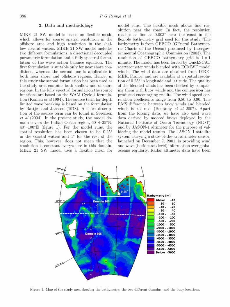
MIKE 21 SW model is based on flexible mesh,which allows for coarse spatial resolution in theoffshore area and high resolution in the shal-low coastal waters. MIKE 21 SW model includestwo different formulations: a directional decoupledparametric formulation and a fully spectral formu-lation of the wave action balance equation. Thefirst formulation is suitable only for near shore con-ditions, whereas the second one is applicable inboth near shore and offshore regions. Hence, inthis study the second formulation has been used asthe study area contains both shallow and offshoreregions. In the fully spectral formulation the sourcefunctions are based on the WAM Cycle 4 formula-tion (Komen et al 1994). The source term for depthlimited wave breaking is based on the formulationby Battjes and Janssen (1978). A short descrip-tion of the source term can be found in Sørensenet al (2004). In the present study, the model do-main covers the Indian Ocean region, 60◦S–25◦N;40◦–100◦E (figure 1). For the model runs, thespatial resolution has been chosen to be 0.25◦

in the coastal waters and 1◦ for the rest of theregion. This, however, does not mean that theresolution is constant everywhere in this domain.MIKE 21 SW model uses a flexible mesh for

model runs. The flexible mesh allows fine res-olution near the coast. In fact, the resolutionreaches as fine as 0.003◦ near the coast in theflexible bathymetry grid used for this study. Thebathymetry is from GEBCO (GEneral Bathymet-ric Charts of the Ocean) produced by Intergov-ernmental Oceanographic Commission (2003). Theresolution of GEBCO bathymetry grid is 1× 1minute. The model has been forced by QuickSCATscatterometer winds blended with ECMWF modelwinds. The wind data are obtained from IFRE-MER, France, and are available at a spatial resolu-tion of 0.25◦ in longitude and latitude. The qualityof the blended winds has been checked by compar-ing them with buoy winds and the comparison hasproduced encouraging results. The wind speed cor-relation coefficients range from 0.80 to 0.90. TheRMS difference between buoy winds and blendedwinds is <2 m/s (Bentamy et al 2007). Apartfrom the forcing data, we have also used wavedata derived by moored buoys deployed by theNational Institute of Ocean Technology (NIOT)and by JASON-1 altimeter for the purpose of val-idating the model results. The JASON 1 satellitesystem carrying a state-of-the-art altimeter sensor,launched on December 7, 2001, is providing windand wave (besides sea level) information over globaloceans regularly. Radar altimeter data have been

Figure 1. Map of the study area showing the bathymetry, the two different domains, and the buoy locations.

Wave hindcast experiments in the Indian Ocean 387

provided by the Delft Institute for Earth-OrientedSpace Research Radar Altimeter Database system(http://rads.tudelft.nl/rads/rads.shtml).

3. Model experiments

As mentioned earlier, the basic objective is to carryout hindcasts with MIKE-21 and subsequently tovalidate the hindcasts. For this purpose, the modelhas been earlier calibrated using number of in-situdata of Indian Ocean region and various modelparameters such as breaking parameter, bottomfriction and white capping were tuned to pro-vide better wave predictions. In the experiments,wave breaking parameter (γ = 0.5), bottom friction(Nikuradse roughness) (KN = 0.04 m), and whitecapping coefficients (Cdis = 3.5) were found to beoptimum. And these coefficients have been used inthe experiments performed for the present study.However, in order to fulfill the secondary objectiveof studying the impact of southern ocean waves onthe northern ocean wave characteristics, apart fromthe earlier selected model domain, a smaller one(10◦S–25◦N, 50◦–100◦E) was also selected. Spatialresolution for the smaller domain (Domain 10S)model is identical with that for the larger domain(Domain 60S). The model simulations were per-formed for the year 2005. The wave spectrum isrepresented by 16 direction bins and 25 frequencybins logarithmically spaced from 0.055 to 0.6 Hz.The model derived wave parameters like significantwave height (Hs), swell wave height (Hss), wind seaheight (Hsw), mean wave period (Tm) and meanwave direction (MWD) were compared with similarparameters obtained from NIOT buoys, moored inthe Arabian Sea (AS) and Bay of Bengal (BOB).The locations of the buoys and the period of dataavailability are given in table 1 and the locationsof the buoys are also marked in figure 1.

4. Results and discussions

As mentioned earlier, performance of the modelwas evaluated both in the larger and smallerdomains. We evaluated the performance in termsof significant wave height, swell height, wind seaheight, mean wave period, mean wave direction inboth AS and BOB. In buoy measurements, for seaand swell separation, the wave spectrum measure-ments between 0.04 and 0.1 Hz is considered lowfrequency (swell) components and between 0.1 and0.5 Hz is taken as high frequency (sea) components.Model also follows the same criteria for the seaand swell separation. The definition of mean waveperiod from the buoy is Tm =

√mo/m2. Although

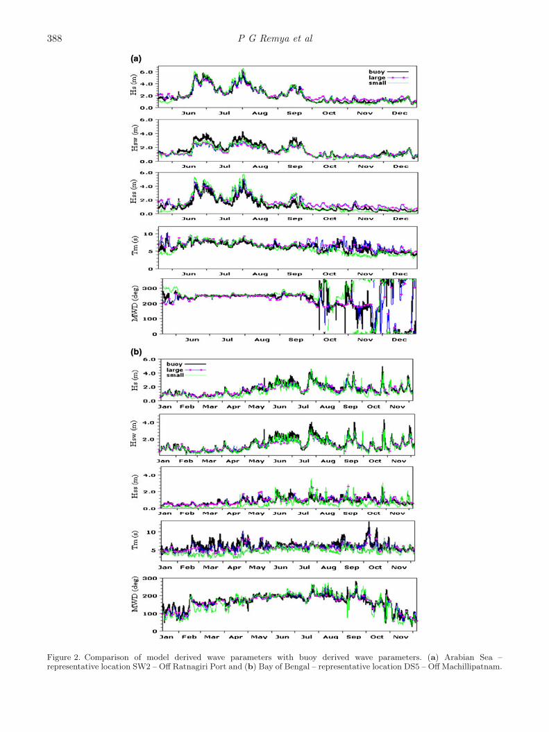
we compared the simulated and observed waveparameters at six different buoy locations for eachof the basins, the results are shown at only one rep-resentative location for each of the basins (figure 2aand b). From figure 2(a), one can conclude that theDomain 60S model consistently overpredicts theswell height in the Arabian Sea except for some iso-lated peaks. This overprediction also affects otherwave parameters like mean wave period and Hsand leads to the unexpected result that the errorstatistics of both the models (Domain 60S one andDomain 10S one) is almost the same. This is astrange result, since the model with the Domain60S including the southern ocean, should, in prin-ciple, have provided simulation of better quality.As seen from figure 2(b), in the case of Bay of Ben-gal, there is significant difference between the twosimulations and the agreement of the Domain 60Sresult with the buoy data is much better.

A possible clue for the poorer performance of themodel in the AS could come from the analysis ofmean wave direction (MWD) at a representativebuoy location (SW2) in the AS. In figure 2, we showthe comparison between simulated and observedMWD. The Arabian Sea experiences three different

Table 1. Locations of buoys with periods of data availability.

Buoy Lat. (N) Long. (E) Period of availability

DS1 15.504 69.276 01/01/2005–26/07/2005

DS4 18.443 87.586 01/01/2005–28/06/2005

DS5 13.991 83.248 01/01/2005–31/12/2005

DS7 8.315 72.661 01/01/2005–31/12/2005

OB3 12.498 72.011 01/01/2005–05/09/2005

OB8 11.503 81.473 01/07/2005–31/12/2005

MB10 12.513 84.983 26/09/2005–31/12/2005

MB11 14.997 87.504 01/01/2005–16/05/2005

SW2 16.985 71.099 13/05/2005–31/12/2005

SW3 15.010 73.021 01/01/2005–30/06/2005

SW4 12.936 74.723 01/01/2005–16/06/2005

SW6 13.183 80.392 05/02/2005–23/08/2005

388 P G Remya et al

Figure 2. Comparison of model derived wave parameters with buoy derived wave parameters. (a) Arabian Sea –representative location SW2 – Off Ratnagiri Port and (b) Bay of Bengal – representative location DS5 – Off Machillipatnam.

Wave hindcast experiments in the Indian Ocean 389

seasons in a year: pre-monsoon (February–May),southwest monsoon (June–September) and north-east monsoon (October–January). It can be seenthat the deviation is more pronounced in pre-monsoon and northeast (NE) monsoon seasons.This finding was true for all the six buoys in the AS.During southwest (SW) monsoon season, the windseas are dominating and this might be the reasonfor the change in performance during SW monsoon.During pre-monsoon season, large scale winds areweak and hence sea breeze has an impact on thediurnal cycle of the sea state along the west coastof India (Neetu et al 2006). Since this sea breezehas not been taken into account by our model,the simulated MWD does not match the observedone. During NE monsoon season, another mecha-nism seems to be at work for the poor match ofthe simulated MWD with observed one. On sev-eral occasions, swells propagating from the north-west were observed. A study of ‘Shamal’ swells car-ried out by Aboobacker et al (2011) showed theimpact of northwest swells on wave conditions offwest coast of India during NE monsoon. In ourstudy, we have closed the land boundary at 25◦Nand have not considered the waves entering intothe Arabian Sea from the Persian gulf. The abovedescribed factors might be the reason for the largedeviation observed in mean wave direction off thewest coast of India during pre-monsoon and NEmonsoon seasons. Thus it is not surprising thateven a Domain 60S model has failed to providesimulation of better quality. In the case of BOBthe agreement between model-derived MWD andbuoy MWD is much better for the Domain 60Smodel simulation (figure 2b). This agreement isnot season- or month-dependent. This supports theconjecture that southern ocean swells cannot beneglected in hindcasts with MIKE-21 model.

Earlier, we have shown only figures for two rep-resentative buoy locations. Now we provide the

detailed statistics for all the six buoy locations,separately for the AS and BOB. Various statis-tical measures like Bias, root mean square error(RMSE), scatter index (SI), correlation coefficient(R) are used to assess the model performance bycomparing the model derived parameters againstthe corresponding buoy observations. The formulaefor the statistical measures are:

Bias =1n

∑(m − obs) (1)

RMSE =

√1n

∑(m − obs)2 (2)

SI = (RMSE) /(obs

)(3)

R =∑

(m − m)(obs − obs

)

√∑(m − m)2

(obs − obs

)2(4)

Here obs is the mean value of a particular waveparameter derived by the buoys in a particularbasin. m is the mean value of the model derivedwave parameter.

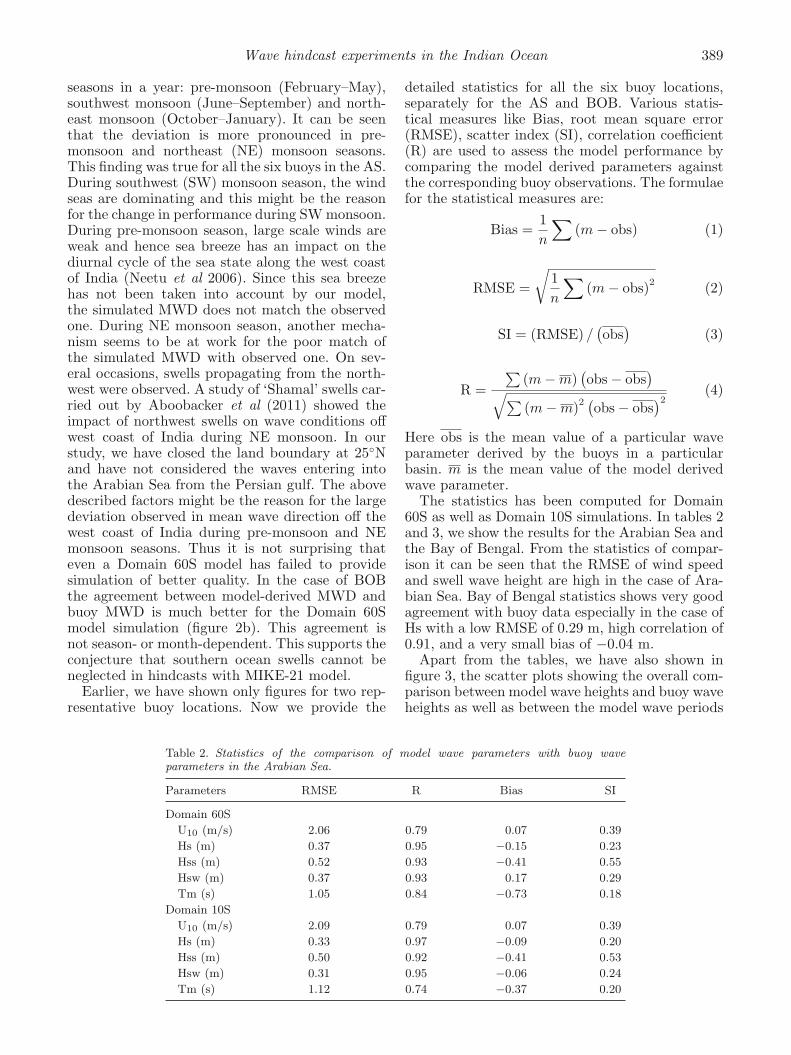
The statistics has been computed for Domain60S as well as Domain 10S simulations. In tables 2and 3, we show the results for the Arabian Sea andthe Bay of Bengal. From the statistics of compar-ison it can be seen that the RMSE of wind speedand swell wave height are high in the case of Ara-bian Sea. Bay of Bengal statistics shows very goodagreement with buoy data especially in the case ofHs with a low RMSE of 0.29 m, high correlation of0.91, and a very small bias of −0.04 m.

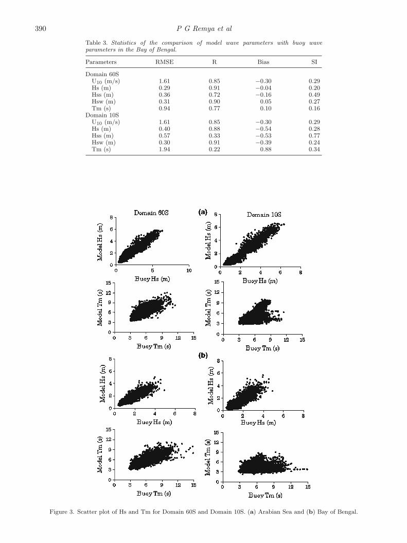
Apart from the tables, we have also shown infigure 3, the scatter plots showing the overall com-parison between model wave heights and buoy waveheights as well as between the model wave periods

Table 2. Statistics of the comparison of model wave parameters with buoy waveparameters in the Arabian Sea.

Parameters RMSE R Bias SI

Domain 60S

U10 (m/s) 2.06 0.79 0.07 0.39

Hs (m) 0.37 0.95 −0.15 0.23

Hss (m) 0.52 0.93 −0.41 0.55

Hsw (m) 0.37 0.93 0.17 0.29

Tm (s) 1.05 0.84 −0.73 0.18

Domain 10S

U10 (m/s) 2.09 0.79 0.07 0.39

Hs (m) 0.33 0.97 −0.09 0.20

Hss (m) 0.50 0.92 −0.41 0.53

Hsw (m) 0.31 0.95 −0.06 0.24

Tm (s) 1.12 0.74 −0.37 0.20

390 P G Remya et al

Table 3. Statistics of the comparison of model wave parameters with buoy waveparameters in the Bay of Bengal.

Parameters RMSE R Bias SI

Domain 60SU10 (m/s) 1.61 0.85 −0.30 0.29Hs (m) 0.29 0.91 −0.04 0.20Hss (m) 0.36 0.72 −0.16 0.49Hsw (m) 0.31 0.90 0.05 0.27Tm (s) 0.94 0.77 0.10 0.16

Domain 10SU10 (m/s) 1.61 0.85 −0.30 0.29Hs (m) 0.40 0.88 −0.54 0.28Hss (m) 0.57 0.33 −0.53 0.77Hsw (m) 0.30 0.91 −0.39 0.24Tm (s) 1.94 0.22 0.88 0.34

Figure 3. Scatter plot of Hs and Tm for Domain 60S and Domain 10S. (a) Arabian Sea and (b) Bay of Bengal.

Wave hindcast experiments in the Indian Ocean 391

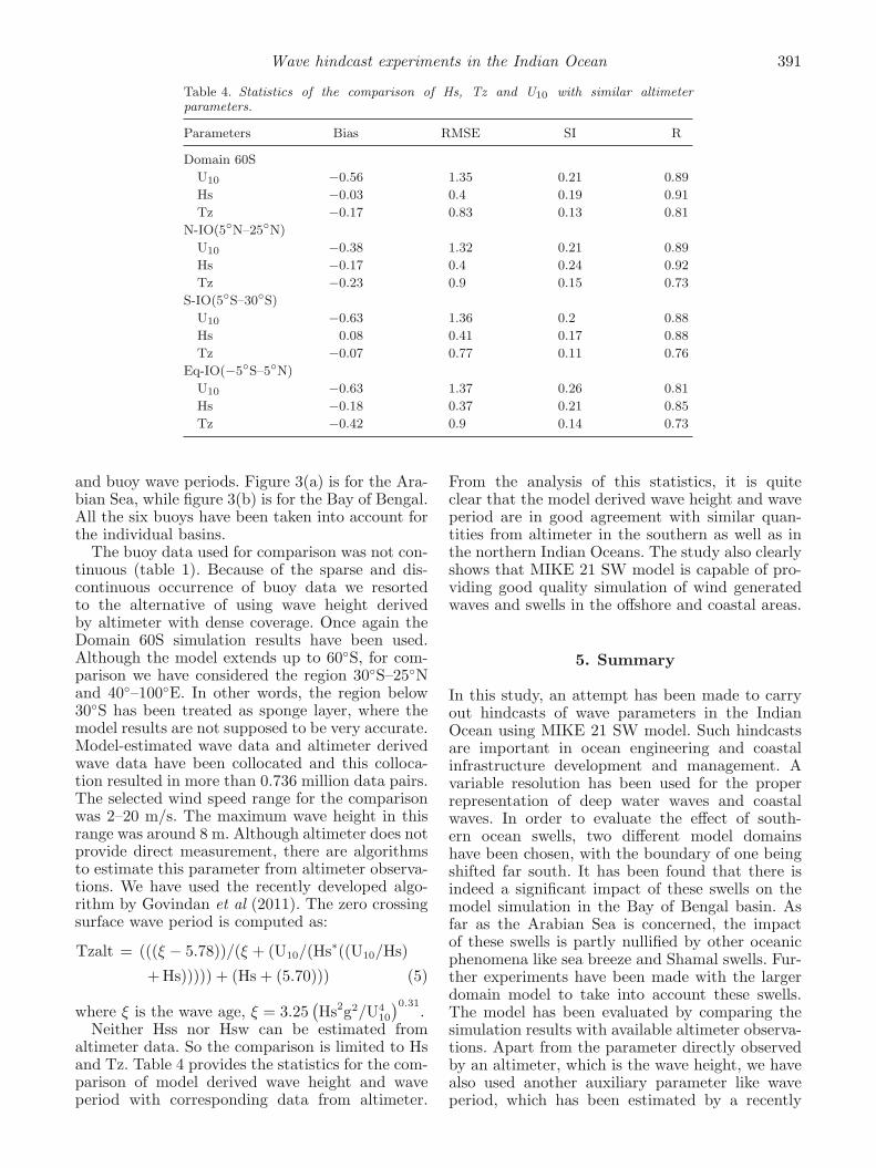
Table 4. Statistics of the comparison of Hs, Tz and U10 with similar altimeterparameters.

Parameters Bias RMSE SI R

Domain 60S

U10 −0.56 1.35 0.21 0.89

Hs −0.03 0.4 0.19 0.91

Tz −0.17 0.83 0.13 0.81

N-IO(5◦N–25◦N)

U10 −0.38 1.32 0.21 0.89

Hs −0.17 0.4 0.24 0.92

Tz −0.23 0.9 0.15 0.73

S-IO(5◦S–30◦S)

U10 −0.63 1.36 0.2 0.88

Hs 0.08 0.41 0.17 0.88

Tz −0.07 0.77 0.11 0.76

Eq-IO(−5◦S–5◦N)

U10 −0.63 1.37 0.26 0.81

Hs −0.18 0.37 0.21 0.85

Tz −0.42 0.9 0.14 0.73

and buoy wave periods. Figure 3(a) is for the Ara-bian Sea, while figure 3(b) is for the Bay of Bengal.All the six buoys have been taken into account forthe individual basins.

The buoy data used for comparison was not con-tinuous (table 1). Because of the sparse and dis-continuous occurrence of buoy data we resortedto the alternative of using wave height derivedby altimeter with dense coverage. Once again theDomain 60S simulation results have been used.Although the model extends up to 60◦S, for com-parison we have considered the region 30◦S–25◦Nand 40◦–100◦E. In other words, the region below30◦S has been treated as sponge layer, where themodel results are not supposed to be very accurate.Model-estimated wave data and altimeter derivedwave data have been collocated and this colloca-tion resulted in more than 0.736 million data pairs.The selected wind speed range for the comparisonwas 2–20 m/s. The maximum wave height in thisrange was around 8 m. Although altimeter does notprovide direct measurement, there are algorithmsto estimate this parameter from altimeter observa-tions. We have used the recently developed algo-rithm by Govindan et al (2011). The zero crossingsurface wave period is computed as:

Tzalt = (((ξ − 5.78))/(ξ + (U10/(Hs∗((U10/Hs)

+ Hs))))) + (Hs + (5.70))) (5)

where ξ is the wave age, ξ = 3.25(Hs2g2/U4

10

)0.31.

Neither Hss nor Hsw can be estimated fromaltimeter data. So the comparison is limited to Hsand Tz. Table 4 provides the statistics for the com-parison of model derived wave height and waveperiod with corresponding data from altimeter.

From the analysis of this statistics, it is quiteclear that the model derived wave height and waveperiod are in good agreement with similar quan-tities from altimeter in the southern as well as inthe northern Indian Oceans. The study also clearlyshows that MIKE 21 SW model is capable of pro-viding good quality simulation of wind generatedwaves and swells in the offshore and coastal areas.

5. Summary

In this study, an attempt has been made to carryout hindcasts of wave parameters in the IndianOcean using MIKE 21 SW model. Such hindcastsare important in ocean engineering and coastalinfrastructure development and management. Avariable resolution has been used for the properrepresentation of deep water waves and coastalwaves. In order to evaluate the effect of south-ern ocean swells, two different model domainshave been chosen, with the boundary of one beingshifted far south. It has been found that there isindeed a significant impact of these swells on themodel simulation in the Bay of Bengal basin. Asfar as the Arabian Sea is concerned, the impactof these swells is partly nullified by other oceanicphenomena like sea breeze and Shamal swells. Fur-ther experiments have been made with the largerdomain model to take into account these swells.The model has been evaluated by comparing thesimulation results with available altimeter observa-tions. Apart from the parameter directly observedby an altimeter, which is the wave height, we havealso used another auxiliary parameter like waveperiod, which has been estimated by a recently

392 P G Remya et al

formulated novel algorithm. All the validationresults point to the fact that the performance ofthe model is quite satisfactory. Hence it can be con-cluded with reasonable confidence that the modelwith this particular configuration can serve thepurpose of reliable wave hindcasts in the IndianOcean region.

Acknowledgements

The authors wish to thank the Director, SpaceApplications Centre, the Deputy Director, Earth,Ocean, Atmosphere, Planetary Sciences and Appli-cations Area and the Group Director, Atmosphericand Oceanic Sciences Group, for the motivationand encouragement. They are also indebted to twoanonymous reviewers for their valuable comments.

References

Aboobacker V M, Vethamony P and Rashmi R 2011‘Shamal’ swells in the Arabian Sea and their influencealong the west coast of India; Geophys. Res. Lett. 38(3)7p, doi: 10.1029/2010GL045736.

Battjes J A and Janssen J P F M 1978 Energy loss andset-up due to wave breaking of random waves; Proc. 16th

International Conference on Costal Engineering, ASCE,pp. 569–587.

Bentamy A, Ayina H L, Queffeulou P and Croize-FillonD 2006 Improved near real time surface wind resolutionover the Mediterranean Sea; Ocean Science Discussion 3435–470.

Bentamy A, Ayina H L, Queffeulou P, Croize-Fillon D andKerbaol V 2007 Improved near real time surface windresolution over the Mediterranean Sea; Ocean Science 3259–271.

DHI 2005 Mike 21 spectral wave module, Scientific documen-tation; Danish Hydraulic Institute (DHI).

Govindan R, Kumar R, Basu S and Sarkar A 2011 Altimeterderived ocean wave period using genetic algorithm; IEEEGeosci. Rem. Sens. Lett. 8 354–358.

IOC 2003 Centenary Edition of the GEBCO Digital Atlas,published on CD-ROM on behalf of the Intergovern-mental Oceanographic Commission and the InternationalHydrographic Centre, Organization as part of the GeneralBathymetric Chart of the Oceans; British OceanographicData Liverpool.

Neetu S, Shetye S and Chandramohan P 2006 Impact of sea-breeze on wind-seas off Goa, west coast of India; J. EarthSyst. Sci. 115 229–234.

Sørensen O R, Kofed-Hansen H, Rugbjerg M and SørensenL S 2004 A third generation spectral wave model usingan unstructured finite volume technique; Proc. 29thInternational Conference on Coastal Engineering, Lisbon,Portugal.

Sverdrup H U and Munk W H 1947 Wind, sea, and swell:Theory of relations for forecasting; US Navy Department,Hydrographic Office Publication no 601, pp. 1–44.

MS received 30 May 2011; revised 11 October 2011; accepted 13 October 2011