Abstract: Light field microscopy is a new technique for high-speedvolumetric imaging of weakly scattering or fluorescent specimens. Itemploys an array of microlenses to trade off spatial resolution againstangular resolution, thereby allowing a 4-D light field to be captured using asingle photographic exposure without the need for scanning. The recordedlight field can then be used to computationally reconstruct a full volume.In this paper, we present an optical model for light field microscopy basedon wave optics, instead of previously reported ray optics models. We alsopresent a 3-D deconvolution method for light field microscopy that is ableto reconstruct volumes at higher spatial resolution, and with better opticalsectioning, than previously reported. To accomplish this, we take advantageof the dense spatio-angular sampling provided by a microlens array at axialpositions away from the native object plane. This dense sampling permitsus to decode aliasing present in the light field to reconstruct high-frequencyinformation. We formulate our method as an inverse problem for recon-structing the 3-D volume, which we solve using a GPU-accelerated iterativealgorithm. Theoretical limits on the depth-dependent lateral resolutionof the reconstructed volumes are derived. We show that these limits arein good agreement with experimental results on a standard USAF 1951resolution target. Finally, we present 3-D reconstructions of pollen grainsthat demonstrate the improvements in fidelity made possible by our method.
References and links1. M. Levoy, R. Ng, A. Adams, M. Footer, and M. Horowitz, “Light field microscopy,” in Proceedings of ACM
SIGGRAPH. (2006) 924–934.2. M. Levoy, Z. Zhang, and I. McDowell, “Recording and controlling the 4D light field in a microscope using
microlens arrays,” Journal of Microscopy 235, 144–162 (2009).3. S. Farsiu, D. Robinson, M. Elad, and P. Milanfar, “Advances and challenges in super-resolution,” International
Journal of Imaging Systems and Technology 14, 47–57 (2004).4. R. Ng, “Fourier slice photography,” in Proceedings of ACM SIGGRAPH (2005). 735–744.5. M. Bertero and C. de Mol, “III Super-resolution by data inversion,” in Progress in Optics (Elsevier, 1996) pp.
129–178.
#193936 - $15.00 USD Received 16 Jul 2013; revised 30 Sep 2013; accepted 4 Oct 2013; published 17 Oct 2013(C) 2013 OSA 21 October 2013 | Vol. 21, No. 21 | DOI:10.1364/OE.21.025418 | OPTICS EXPRESS 25418
6. T. Pham, L. van Vliet, and K. Schutte, “Influence of signal-to-noise ratio and point spread function on limits ofsuperresolution,” Proc. SPIE 5672, 169–180 (2005).
7. S. Baker and T. Kanade, “Limits on super-resolution and how to break them,” IEEE Trans. Pattern Anal. Mach.Intell. 24. 1167–1183 (2002)
8. K. Grochenig and T. Strohmer, “Numerical and theoretical aspects of nonuniform sampling of band-limitedimages,” in “Nonuniform Sampling,” , F. Marvasti, ed.. Information Technology: Transmission, Processing, andStorage, 283–324 (Springer US, 2010).
9. T. Bishop and P. Favaro, “The light field camera: extended depth of field, aliasing and super-resolution,” IEEETrans. Pattern Anal. Mach. Intell. 34. 972–986 (2012).
10. W. Chan, E. Lam, M. Ng, and G. Mak, “Super-resolution reconstruction in a computational compound-eye imag-ing system,” Multidimensional Systems and Signal Processing 18. 83–101. (2007).
11. M. Gu, Advanced Optical Imaging Theory (Springer, 1999).12. D. A. Agard, “Optical sectioning microscopy: cellular architecture in three dimensions,” Annual review of bio-
physics and bioengineering 13, 191–219. (1984).13. M. Born and E. Wolf, Principles of Optics, 7th ed. (Cambridge University, 1999).14. M. R. Arnison and C. J. R. Sheppard, “A 3D vectorial optical transfer function suitable for arbitrary pupil func-
tions,” Optics communications 211, 53–63 (2002).15. A. Egner and S. W. Hell, “Equivalence of the Huygens–Fresnel and Debye approach for the calculation of high
aperture point-spread functions in the presence of refractive index mismatch,” Journal of Microscopy 193, 244–249 (1999).
16. J. Breckinridge, D. Voelz, and J. B. Breckinridge, Computational Fourier Optics: a MATLAB Tutorial (SPIEPress, 2011).
17. J. M. Bardsley and J. G. Nagy, “Covariance-preconditioned iterative methods for nonnegatively constrainedastronomical imaging,” SIAM journal on matrix analysis and applications 27, 1184–1197 (2006).
18. M. Bertero, P. Boccacci, G. Desidera, and G. Vicidomini, “Image deblurring with Poisson data: from cells togalaxies,” Inverse Problems 25, 123006 (2009).
19. S. Shroff and K. Berkner, “Image formation analysis and high resolution image reconstruction for plenopticimaging systems,” Applied optics, 52, D22D31, (2013).
20. J. Rosen, N. Siegel, and G. Brooker, “Theoretical and experimental demonstration of resolution beyond theRayleigh limit by FINCH fluorescence microscopic imaging,” Opt. Express 19, 1506–1508 (2011).
21. I. J. Cox and C. J. R. Sheppard, “Information capacity and resolution in an optical system,” J. Opt. Soc. Am. A3, 1152 (1986).
22. R. Heintzmann, “Estimating missing information by maximum likelihood deconvolution,” Micron 38, 136–144(2007)
23. P. Favaro, “A split-sensor light field camera for extended depth of field and superresolution,” in “SPIE ConferenceSeries,” 8436. (2012).
24. C. H. Lu, S. Muenzel, and J. Fleischer, “High-resolution light-field microscopy,” in “Computational OpticalSensing and Imaging, Microscopy and Tomography I (CTh3B),” (2013).
25. S. Abrahamsson, J. Chen, B. Hajj, S. Stallinga, A. Y. Katsov, J. Wisniewski, G. Mizuguchi, P. Soule, F. Mueller,C. D. Darzacq, X. Darzacq, C. Wu, C. I. Bargmann, D. A. Agard, M. G. L. Gustafsson, and M. Dahan, “Fastmulticolor 3D imaging using aberration-corrected multifocus microscopy,” Nat. Meth. 1–6. (2012).
26. M. Pluta, Advanced Light Microscopy, Vol. 1. (Elsevier, 1988).27. J. Goodman, Introduction to Fourier Optics, 2nd ed. (MaGraw-Hill, 1996).
1. Introduction
Light field microscopy [1, 2] is a new approach for rapid, scanless volumetric imaging us-ing optical microscopy. By introducing a microlens array into the light path of a conventionalmicroscope, it is possible to image both the lateral and angular distribution of light passingthrough the specimen volume. This raw spatio-angular data, referred to as a light field, can bepost-processed in software to produce a full 3-D reconstruction of the object. Because the lightfield is captured in a snapshot at a single instant in time, light field microscopy makes it possibleto perform scanless volumetric imaging at the frame rate of the camera.
However, scanless 3-D imaging with a light field microscope (LFM) comes at a cost: lateralspatial resolution must be sacrificed to record angular information. This angular information iswhat permits volumetric reconstruction, so this is equivalent to a trade off between lateral andaxial resolution. In previous work [1], we concluded that this loss of lateral resolution is exactlyproportional to the number of discrete angular samples collected. This in turn is proportional
#193936 - $15.00 USD Received 16 Jul 2013; revised 30 Sep 2013; accepted 4 Oct 2013; published 17 Oct 2013(C) 2013 OSA 21 October 2013 | Vol. 21, No. 21 | DOI:10.1364/OE.21.025418 | OPTICS EXPRESS 25419
to the number of pixels behind each lenslet in the array. Since it is desirable to record manyangular samples at each spatial position (typically greater than 10 in each angular direction),this represents a considerable resolution loss relative to the diffraction limited performance ofa conventional wide-field fluorescence microscope.
In this paper we present a novel approach for light field reconstruction with improved lateralspatial resolution compared to ordinary light field microscopy. We further show that, whenconstraining the reconstruction to a single z-plane in the case of a planar test target, we achieveup to an 8-fold improvement in resolution over previously reported limits (see Fig. 1). Thisis achieved by modeling the spatially varying point spread function of the LFM using waveoptics and using this model to perform 3-D deconvolution. Such deconvolution mitigates theproblem of decreased lateral resolution, thereby addressing one of the main drawbacks of lightfield microscopy.
This resolution enhancement is possible because the sampling rate provided by the lenslets iswell below the optical band limit of the microscope. As a result, the microlens array samples the
Optical defocus in a conventional
microscope(ground truth)
z = 0µm(Native Object Plane)
z = -20µm z = -50µm z = -100µm
(c)
(b)
(a)
Computationallyrefocusedlight field
(2009 method)
Light field deconvolution
(our new method)
Fig. 1. USAF 1951 resolution test target translated to depths below the native object plane(z = 0 µm) and imaged using a light field microscope with a 20x 0.5NA water-dippingobjective. (a) Photographs taken with a conventional microscope as the target is translatedto the z-heights denoted below each image. (b) Computational re-focusing using our 2009method [2] while the microscope was defocused to the same heights as (a). While somecomputational refocusing is possible, there has been a significant loss of lateral resolution.(c) The reconstruction algorithm presented in this paper brings the target back into focus,achieving up to an 8-fold improvement in lateral resolution compared to (b) except at thenative object plane (left image).
#193936 - $15.00 USD Received 16 Jul 2013; revised 30 Sep 2013; accepted 4 Oct 2013; published 17 Oct 2013(C) 2013 OSA 21 October 2013 | Vol. 21, No. 21 | DOI:10.1364/OE.21.025418 | OPTICS EXPRESS 25420
optical signal below the Shannon-Nyquist limit, causing high frequency features to be aliasedin the light field. In conventional imaging, such aliasing is undesirable because it irreversiblycorrupts the recorded image. However, in light field imaging, aliasing is actually beneficial. Inparticular, the light field’s angular samples, when projected into the volume, create a dense,non-uniform sampling pattern that allows us to “decode” aliased information during 3-D de-convolution.
The reconstruction technique we have developed is closely related to “computational super-resolution” methods in the field of computer vision [3]. This signal processing technique com-bines multiple under-sampled and aliased images of a scene to recover an image with sub-pixel(or in our case, sub-lenslet) resolution. Note that the computational super-resolution we de-scribe here is not to be confused with optical “super-resolution” or “super-localization” meth-ods in microscopy such as Structure Illumination Microscopy (SIM), Photo Activated Local-ization Microscopy (PALM), and Stochastic Optical Reconstruction Microscopy (STORM),which seek to surpass the diffraction limit. Computational super-resolution has recently beenexplored in light field photography, and shown to be effective at recovering resolution in themanner described above. However, these algorithms make assumptions typical at macroscopicphotographic scales: namely opaque scenes and diffusely reflecting objects. They also modellight using ray optics. These assumptions do not hold when imaging microscopic samples.
This paper builds on this past work, making several contributions. First, we present a waveoptics model that accounts for the diffraction effects that occur when recording the light fieldwith a microscope. We then explain how this optical model can be used in a deconvolution al-gorithm for 3-D volume reconstruction. This approach is suitable for fluorescence microscopy,where the volume to be reconstructed is largely transparent (i.e. with minimal scattering orabsorption). Finally, we characterize the lateral resolution limit in light field microscopy, anddiscuss how optical design choices affect these resolution limits. To aid in exploring thesetrade-offs, we propose a theoretical band limit that should prove useful when choosing whichobjective, microlens array, and camera sensor to use for a given 3-D imaging scenario.
2. Background
2.1. 3-D imaging with the light field microscope
A conventional microscope can be converted into a light field microscope by placing a mi-crolens array at the native image plane as shown in Fig. 2(a). Light field imaging can beperformed using any microscope objective so long as the f-number of the microlens array ismatched to the numerical aperture of the objective. This design choice ensures that the imagingcircles behind the lenslets exactly tile the image plane without overlapping or leaving spaces inbetween them [1]. The camera sensor is placed behind the lenslets at a distance of one lensletfocal length—typically 1 to 10-mm. This is not practical for most commercial sensors, whichare recessed inside the body of the camera, but it is possible to use a relay lens system placedin between the camera and the microlens array to re-image the lenslets’ back focal plane ontothe sensor. For example, we use a relay lens formed by a pair of photographic lenses mountedface-to-face via a filter ring adaptor.
Figures 2(b) and 2(c) depict simplified ray optics diagrams that are useful for building in-tuition about light propagation through the LFM. Figure 2(b) shows a ray bundle from a pointemitter on the native object plane (i.e. the plane the is normally in focus in a widefield mi-croscope). Rays emitted at different angles within the numerical aperture of the objective arerecorded by separate pixels on the sensor. Summing the pixels shown in red yields the samemeasurement that would have resulted if the camera sensor itself had been placed at the na-tive image plane (i.e. the image plane of a widefield microscope that is conjugate to the native
#193936 - $15.00 USD Received 16 Jul 2013; revised 30 Sep 2013; accepted 4 Oct 2013; published 17 Oct 2013(C) 2013 OSA 21 October 2013 | Vol. 21, No. 21 | DOI:10.1364/OE.21.025418 | OPTICS EXPRESS 25421
object plane) and binned to have a pixel that is the size of a lenslet. That is, summing the pix-els behind each lenslet yields an image focused at the native object plane, albeit with greatlyreduced lateral resolution equal to the diameter of one lenslet. Figure 2(c) shows how light iscollected from a point emitter below the native object plane. Here the light is focused by themicrolens array into a pattern of spots on the sensor. This pattern spreads out as the point movesfurther from the native object plane. Given a model of this spreading pattern, it is possible tosum together the appropriate light field pixels to produce a computationally refocused image(refer to [1] and [4] for more details).
Sensor Plane|h (x,p)|2
Native Image PlaneUi (x,p)
Tube Lens
Objective
Native Object Plane
fobj fobj ftl ftl fµlens
Microlens Array
Image SensorTube LensObjective
Origin
+z
+x
BackAperture
(Telecentric Stop)
Ideal point source at p
(a) (b) (c)
(e)Fourier Plane
Uf (x,p)Native Object Plane
Uo (x,p)
Native Image Plane
(d)
+x
+y
Simulated light field
Experimental light field
125 µm
125 µm
Image Space
+x
+y
Image Space
Fig. 2. Optical model of the light field microscope. (a) A fluorescence microscope can beconverted into a light field microscope by placing a microlens array at the native imageplane. (b) A ray-optics schematic indicating the pattern of illumination generated by onepoint source. The gray grid delineates pixel locations, and the white circles depict the back-aperture of the objective imaged onto the sensor by each lenslet. Red level indicates theintensity of illumination arriving at the sensor. For a point source on the native object plane(red dot), all rays pass through a single lenslet. (c) A point source below the native objectplane generates a more complicated intensity pattern involving many lenslets. (d) A reallight field recorded on our microscope using a 60x 1.4NA oil objective and a 125 µm pitchf/20 microlens array of a 0.5 µm fluorescent bead placed 4 µm below the native object plane.Diffraction effects are present in the images formed behind each lenslet. (e) A schematic ofour wave optics model based on the LFM optical path (not drawn to scale). In this model,the microlens array at the native image plane is modeled as a tiled phase mask operating onthis wavefront, which is then propagated to the camera sensor. The xy cross section on thefar right shows the simulated light field generated at the sensor plane. The simulation is ingood agreement with the experimentally measured light field in (d).
#193936 - $15.00 USD Received 16 Jul 2013; revised 30 Sep 2013; accepted 4 Oct 2013; published 17 Oct 2013(C) 2013 OSA 21 October 2013 | Vol. 21, No. 21 | DOI:10.1364/OE.21.025418 | OPTICS EXPRESS 25422
Of course, light is not collected in the simple manner that the schematics in Figs. 2(b) and2(c) would suggest. Diffraction effects are evident upon inspection of a real light field recordedby a LFM (Fig. 2(d)), so a full wave optics treatment is necessary. Figure 2(e) shows a morerealistic optical diagram, along with a simulated intensity distribution of light for a point sourceoff the native object plane. This diagram was produced using our wave optics model. In Section3 we will turn our attention to the details of this model and its implementation, but first webuild more intuition about the 3-D reconstruction problem.
2.2. Light field imaging as limited-angle tomography
In light field microscopy, as with other imaging modalities, removing out of focus light from areconstructed volume is accomplished by characterizing the microscope’s point spread function(PSF) and using it to perform 3-D deconvolution. In the appendix of [1] it is shown that, for lightfield microscopy of a relatively transparent sample, 3-D deconvolution is equivalent to solving alimited-angle tomography problem. Figure 3(a) illustrates this connection. An oblique parallelprojection through the sample is collected along chief rays (blue lines) corresponding to thepixels on the left-most side of each lenslet. If we take these blue pixels and use them to forman image, then we will have a low-resolution view of the specimen volume at a certain angle.In essence, this is the image that would be captured by placing a pinhole at a certain location inthe back aperture of the microscope. Hence, we refer to this image as a “pinhole view.”
A light field with N×N pixels behind each lenslet will contain pinhole views at N2 differentangles covering the numerical aperture of the microscope objective. This suggests that lightfield microscopy is essentially a simultaneous tomographic imaging technique in which all N2
projections are collected at once as pinhole views. Thus, successful deconvolution amounts to
(a)
z = 0µmz = -10µmz = -35µmz = -60µmz = -93µm z = -75µm
0 50 100-25 25 75-50-75-100z position (µm)
-125 125
0
x po
sitio
n (µ
m) 10
(c)
20
-20
-10
(b)
6.25 µm
Native Object Plane
+z
+x
Object Space
Native Object Plane
Fig. 3. Sampling of the volume recorded in a microlens-based light field. (a) A bundle oflenslet chief rays captured by the same pixel position relative to each lenslet (blue pixels)form a parallel projection through the volume, providing one of many angular views neces-sary to perform 3-D deconvolution. (b) When lenslet chief rays passing through every pixelin the light field are simultaneously projected back into the object volume, these rays crossat a diversity of x-positions (readers are encouraged to zoom into this figure in a PDF file tosee how this pattern evolves with depth). This dense sampling pattern permits 3-D decon-volution with resolution finer than the lenslet spacing. The only place where this diversitydoes not occur is close to the native object plane; here resolution enhancement is not pos-sible. (c) The distribution of the lenslet chief rays in xy cross-sections of the object volumechanges at different distances from the native object plane. The outline of the lenslets areshown in light gray for scale. At z = 0 µm (rightmost image), the lack of spatial diversityin sample locations is evident.
#193936 - $15.00 USD Received 16 Jul 2013; revised 30 Sep 2013; accepted 4 Oct 2013; published 17 Oct 2013(C) 2013 OSA 21 October 2013 | Vol. 21, No. 21 | DOI:10.1364/OE.21.025418 | OPTICS EXPRESS 25423
fusing these low resolution views to create a high resolution volumetric reconstruction.How much resolution can be recovered in such a reconstruction? This depends in part on
the band limit of the optical signal recorded by each pinhole view; i.e. the amount of low-passfiltering that the optical signal undergoes before it is sampled and digitized. In particular, each“pixel” in a pinhole view corresponds to one lenslet in the microlens array. Lenslets have asquare aperture that acts as a (rect-shaped) band limiting filter. This induces optical blurring,and it is this blurring as well as the blurring due to diffraction that limits the highest spatialfrequency that can be resolved in a pinhole view. When performing full 3-D deconvolution,high frequency details at a certain depth in the volume can only be reconstructed if they can beresolved in the pinhole views. Therefore, the band limits of pinhole views directly determinehow much resolution can be recovered at any given z-plane.
In addition to the band limit, the spatial sampling rate within a pinhole view plays a key rolein determining how high frequency content is recorded in the light field. In each pinhole view,the effective sampling rate is equal to the lenslet pitch divided by the objective magnification.For example, a 125 µm pitch array and a 20x microscope objective will result in a samplingperiod of 6.25 µm. When we present our results in Section 4, we will show that this samples thelight field significantly below its band limit. As a result, high frequency details are aliased inindividual pinhole views. While it may seem that such aliasing would be highly undesirable, itturns out that this is the key to enhancing resolution during 3-D deconvolution. To understandwhy this is the case, we now turn for insight to the field of computational super-resolution.
2.3. Aliasing and computational super-resolution
Computer vision researchers know that multiple aliased, low-resolution images of a scene canbe computationally combined to recover a higher resolution image [3]. Early incarnations ofthis computational super-resolution involved capturing several images while a camera sensorwas translated through random, sub-pixel movements. During each acquisition, high frequencyinformation from the scene is aliased and recorded as low frequency image features in a waythat is uniquely determined by the camera position. If the camera’s trajectory can be accu-rately estimated, then the different, aliased copies of the scene can be combined to form ahigh resolution image. Although not required, deconvolution is often carried out as part of thereconstruction to de-blur the super-resolved image and further enhance its resolution [5].
However, as alluded to in the previous section, there are fundamental limits on the amountof recoverable resolution. In photography, the band limit is determined by the diffraction limitand the size and fill factor of the camera pixels [6]. Since modern image sensors with high fillfactors are very close to band-limited, the achievable super-resolution factor is roughly 2x withdeconvolution, although higher super-resolution factors can be achieved by leveraging priorsthat capture statistical properties of the image being reconstructed [7]. In microscopy, camerapixels are typically chosen to be smaller than the diffraction limit of the microscope objective,so little if any aliasing occurs and computational super-resolution is of limited use.
Of course, in order for high frequency information to be recoverable, enough distinct lowresolution images (each with a different pattern of aliasing) must be recorded. This amountsto a sampling requirement: the sub-pixel shifts between the images must result in a samplingpattern that is dense enough to support reconstruction of the super-resolution image. An in-depth discussion of this sampling requirement is beyond the scope of this paper, but we referthe interested reader to [8].
Super-resolution methods have recently been explored in light field photography, with severalpapers demonstrating that a significant resolution enhancement can be achieved by combiningaliased pinhole views [9, 10]. In microlens-based light fields, the geometry of the optics resultsin a fixed, sub-lenslet sampling pattern that takes the place of the sub-pixel camera movements
#193936 - $15.00 USD Received 16 Jul 2013; revised 30 Sep 2013; accepted 4 Oct 2013; published 17 Oct 2013(C) 2013 OSA 21 October 2013 | Vol. 21, No. 21 | DOI:10.1364/OE.21.025418 | OPTICS EXPRESS 25424
in traditional computational super-resolution. This pattern evolves with depth as depicted inFig. 3(b). At z-planes where samples are dense relative to the spacing between the lenslets, itis possible to combine pinhole views to recover resolution up to the band limit. However, thereare depths where the samples are redundant, most notably at the native object plane (althoughpartial redundancy can also be seen in the figure at z = 72 µm and z = 109 µm). At thesedepths the sampling requirement may not be met, and super-resolution cannot always be fullyrealized. This is why the z = 0 µm plane in Fig. 1(c) remains a low-resolution, aliased imagedespite having been processed by our deconvolution algorithm.
3. Light field deconvolution
With this background in mind, we turn our attention to reconstructing a 3-D volume from a lightfield. In particular, we will solve the following inverse problem: given a light field recorded bya noisy imaging sensor, estimate the radiant intensity at each point in the volume that generatedthe observation. Concretely, we seek to invert the discrete linear forward imaging model,
f = H g, (1)
where the vector f represents the light field, the vector g is the discrete volume being recon-structed, and H is a measurement matrix modeling the forward imaging process. The coeffi-cients of H are largely determined by the point spread function of the light field microscope.Our first task will be to develop a model for this point spread function.
3.1. The light field PSF
The diffraction pattern generated by an ideal point source when passed through an optical sys-tem is the system’s impulse response function, more commonly referred to as the point spreadfunction. In an optical microscope this is the well-known Airy pattern (or its generalization asa double-cone for 3-D imaging) [11].
In the light field microscope a point source generates a more complex diffraction pattern. Anexample of one such “light field point spread function” is shown in Fig. 2(e). These patternscarry considerable information about the 3-D position of a point emitter in the volume, andthis is the basis of our 3-D reconstruction algorithm. Unlike the Airy pattern, which is invariantwith respect to the position of the point source, the light field PSF is translationally-variant.Specifically, the diffraction pattern behind the microlens array changes depending on the 3-Dposition of the point source. This gives rise to two challenges: (1) we must compute a uniquePSF for each point in the volume, and (2) we cannot model optical blurring from the PSF asa convolution, as is commonly done in the case of conventional image formation models [12].Instead, the wavefront recorded at the image sensor plane in Fig. 2(e) is described using a moregeneral linear superposition integral
f (x) =∫|h(x,p)|2 g(p)dp, (2)
where p ∈ R3 is the position in a volume containing isotropic emitters whose combined in-tensities are distributed according to g(p). When imaged, this volume gives rise to continuous2-D intensity pattern f (x) at the image sensor plane. The optical impulse response h(x,p) is afunction of both the position p in the volume being imaged as well as the position x ∈ R2 onthe sensor plane.
Notice that Eq. (2) is the continuous version of Eq. (1). We use the squared modulus of h(x,p)in Eq. (2) because fluorescence microscopy is an incoherent, and therefore linear, imagingprocess. Although light from a single point emitter produces a coherent interference pattern
#193936 - $15.00 USD Received 16 Jul 2013; revised 30 Sep 2013; accepted 4 Oct 2013; published 17 Oct 2013(C) 2013 OSA 21 October 2013 | Vol. 21, No. 21 | DOI:10.1364/OE.21.025418 | OPTICS EXPRESS 25425
(and therefore the function h(x,p) is a complex field containing both amplitude and phaseinformation), coherence effects between any two point sources average out to a mean intensitylevel due to the rapid, random fluctuations in the emission time of different fluorophores. As aresult, there are no interference effects when light from two sources interact; their contributionson the image sensor are simply the sum of their intensities.
Additionally, in the interest of practicality and computational efficiency we make two as-sumptions about the nature of the light and volume being imaged. First, we assume that thelight is monochromatic with a wavelength λ . This approximation is reasonably accurate forfluorescent imaging with a narrow wavelength emission filter. Second, our model adopts thefirst Born approximation [13], i.e. it assumes that there is no scattering in the volume. Onceemitted, the light from a point is assumed to radiate as a perfect spherical wavefront until itarrives at the microscope objective. This approximation holds up well when imaging a vol-ume free of occluding or heavily scattering objects. However, performance does degrade whenimaging deep into weakly scattering samples or into samples with varying indices of refraction.Modeling these effects is the subject of future work.
Figure 2(e) shows the optical path of the light field microscope in detail. With the objectiveand tube lens configured as a 4-f system, the back aperture of the objective serves as a telecentricstop, making the microscope both object side and image side telecentric. The focal length ofthe tube lens ftl varies by microscope manufacturer ( ftl = 200mm for our Nikon microscope),and the focal length of the objective can be computed from the magnification of the objectivelens: fob j = ftl/M.
An analytical model for the wavefront at the native image plane Ui(x,p) generated by a pointsource at p can be computed using scalar Debye theory [11]. For an objective with a circularaperture, a point source at p = (p1, p2, p3) produces a wavefront at the native image planedescribed by the integral,
Ui(x,p) =M
f 2ob jλ
2 exp(− iu
4 sin2(α/2)
)∫
α
0P(θ) exp
(− iu sin2(θ/2)
2 sin2(α/2)
)J0
(sin(θ)sin(α)
v)
sin(θ)dθ (3)
where J0(·) is the zeroth order Bessel function of the first kind, and ρ is the normalized radiusfrom the center of the pupil. The variables v and u represent normalized radial and axial opticalcoordinates,
v ≈ k√(x1− p1)2 +(x2− p2)2 sin(α)
u ≈ 4k p3 sin2 (α/2) .
The half-angle of the numerical aperture α = sin−1(NA/n) and the wave number k = 2πn/λ
are computed using the emission wavelength λ and the index of refraction n of the sample.The function P(θ) is the apodization function of the microscope. For Abbe-sine corrected ob-jectives, P(θ) =
√cos(θ). Note that Eq. (3) only holds for low to moderate NA objectives. A
vectorial diffraction theory [14, 15] could instead be substituted into our model to enable lightfield reconstruction with high NA objectives. A derivation of these equations and discussion ofpotential extensions, such as the ability to model aberrations, can be found in [11].
Having computed the scalar wavefront at the native image plane, we next account for thefocusing of light through the microlens array. Our microlens arrays contain square-truncated
#193936 - $15.00 USD Received 16 Jul 2013; revised 30 Sep 2013; accepted 4 Oct 2013; published 17 Oct 2013(C) 2013 OSA 21 October 2013 | Vol. 21, No. 21 | DOI:10.1364/OE.21.025418 | OPTICS EXPRESS 25426
lenslets (meaning that their aperture is square) with a 100% fill factor. Consider a single lensletcentered on the optical axis with focal length fµlens and pitch d. This lenslet can be modeled asan amplitude mask representing the lenslet aperture and a phase mask representing the refrac-tion of light through the lenslet itself:
φ(x) = rect(x/d) exp(−i k
2 fµlens‖x‖2
2
). (4)
The same amplitude and phase mask is applied in a tiled fashion to the rest of the incomingwavefront. Application of the full, tiled microlens array can be described as a convolution of a2-D comb function with φ (x):
Φ(x) = φ(x)∗ comb(x/d).
Next, the wavefront propagates a distance of fµlens from the native image plane to the sensorplane. The lenslets used in the LFM have a Fresnel number between 1 and 10, so Fresnelpropagation is an accurate and computationally attractive approach for modeling light transportfrom the microlens array to the sensor [16, p.55]. The final light field PSF can thus be computedusing the Fourier transform operator F{·} as
h(x,p) = F−1{
F {Φ(x)Ui(x,p)} exp[− i
4πλ fµlens (ω
2x +ω
2y )
]}, (5)
where the exponential term is the transfer function for a Fresnel diffraction integral, and ωx andωy are spatial frequencies along the x and y directions in the sensor plane.
3.2. Discretized optical model
We now describe how to discretize Eq. (2) to produce Eq. (1), which can then be solved on adigital computer. The sensor plane wavefront f (x) is sampled by a camera containing Np pixels.To simplify the notation, we re-order these pixels into a vector f ∈ ZNp
+ . Similarly, during 3-Ddeconvolution the volume g(p) is sub-divided into Nv = Nx×Ny×Nz voxels and re-orderedinto a vector g ∈RNv
+ (see Fig. 4).Although the dimensionality of f is fixed by the number of pixels in the image sensor, the
dimensionality of g (i.e. the sampling rate of the reconstructed volume) is adjustable in ouralgorithm. Clearly, the sampling rate should be high enough to capture whatever informationcan be reconstructed from the light field. However, oversampling will lead to a rapid increasein computational cost without any real benefit. We will be explicit about our choice of volumesampling rates when we present results in Section 4, but here we will establish the followinguseful definition. A volume sampled at the “lenslet sampling period” has voxels with a spacingequal to the lenslet pitch d divided by the objective magnification M. For example, when imag-ing with a 125 µm pitch microlens array and a 20x microscope objective, the lenslet samplingperiod would be 6.25 µm. In this paper, we will sample the volume more finely at a rate that isa “super-sample factor” s ∈ Z times the lenslet sampling rate (where the lenslet sampling rateis the reciprocal of the lenslet sampling period). The sampling rate of the volume is thereforesM/d. Continuing our example, a reconstruction with super-sample factor s = 16 would resultin a volume with voxels spaced by 0.39 µm. We refer to this as a volume that is sampled at 16xthe lenslet sampling rate.
To complete our discrete model, we form a measurement matrix H whose coefficients hi jindicate the proportion of the light arriving at pixel j from voxel i. Voxels in the reconstructedvolume and pixels on the sensor have finite volume and area, respectively. Therefore the coef-ficients of H are computed via a definite integral over the continuous light field PSF,
#193936 - $15.00 USD Received 16 Jul 2013; revised 30 Sep 2013; accepted 4 Oct 2013; published 17 Oct 2013(C) 2013 OSA 21 October 2013 | Vol. 21, No. 21 | DOI:10.1364/OE.21.025418 | OPTICS EXPRESS 25427
hi j =∫
α j
∫βi
wi(p) |h(x,p)|2 dpdx (6)
where α j is the area for pixel j, and βi is the volume for voxel i. We assume that pixels aresquare and have have a 100% fill factor, which is a good approximation for modern scientificimage sensors. Voxel i is integrated over a cubic volume centered at a point pi.
Equation (6) is a resampling operation, thus we must be careful not to introduce aliasingin the volume when discretizing Eq. (2). The resampling filter wi(p) that weights the PSFcontribution at the center of a voxel more than the at its edges is introduced for this purpose. Inour implementation we use a Hann (i.e. raised cosine) window with width equal to two timesthe volume sampling period, although a different resampling filter could be used if desired. Wefound the exact choice of resampling filter to be incidental to the algorithm; once the voxelsampling rate surpasses the band limit discussed in Sec. 2.2, the choice of resampling filter haslittle impact on the quality of the reconstruction.
Figure 4(a) shows that the columns of H contain the discrete versions of the light field pointspread functions. That is, column i contains the forward projection generated when a singlenon-zero voxel i is projected according to Eq. (1). In Fig. 4(b) we see that the rows of H (oralternatively the columns of HT ) also have an interesting interpretation. We call these pixel
. . . . . . . .
. . . . . . . .
. . . . . . . .
. . . . . . . .
. . . . . . . .
z position (µm)
Pixel backprojection for pixel j(b)
+z
+y
-50 0 50 100-100
f = H g.....
=
.
.
.
.
.
.
.
.
Light field PSF for voxel i(a)
Light Field Measurement Matrix Volume
Nv x 1 Np x 1
voxel i
pixel j
Np x Nv
+x
+y
Image Space
Object Space
125 µm
6.25 µm
Fig. 4. The discrete light field imaging model, prior to accounting for sensor noise. Thedimensionality of the light field f is fixed by the image sensor, but the dimensionality (orequivalently, the sampling rate) of the volume g is a user-selectable parameter in the re-construction algorithm. (a) Column i of the measurement matrix H (purple) contains thediscretized light field point spread function for voxel i, which corresponds to the forwardprojection of that point in the volume. (b) Row j of the measurement matrix (green) con-tains a pixel back projection: a visualization that shows how much each voxel in the volumecontributes to a single pixel j in the light field. The cross sections in this figure were com-puted using our wave optics model for a 20x 0.5NA water dipping objective and a 125µmpitch f/20 microlens array.
#193936 - $15.00 USD Received 16 Jul 2013; revised 30 Sep 2013; accepted 4 Oct 2013; published 17 Oct 2013(C) 2013 OSA 21 October 2013 | Vol. 21, No. 21 | DOI:10.1364/OE.21.025418 | OPTICS EXPRESS 25428
back projections by analogy to back projection operators in tomographic reconstruction algo-rithms, where the transpose of the measurement matrix is conceptualized as a projection of themeasurement back into the volume. A pixel back projection from column j shows the positionand proportion of light in the volume that contributes to the total intensity recorded at pixel jin the light field. In essence, the pixel back projection allows us to visualize the relative weightof coefficients in a single row of H when it operates on a volume g.
3.3. Sensor noise model
Equation (1) is a strictly deterministic description of the light field imaging process and assumesno noise. We next consider how our imaging model can be extended to model the noise that isnecessarily added by real sensor systems. With modern scientific cameras the dominant sourceof noise is photon shot noise, which means that the ith pixel follows Poisson statistics with a rateparameter equal to fi =(Hg)i – i.e. the light intensity incident on the ith pixel. Read noise canbe largely ignored for modern CCD and sCMOS cameras, although it can be added to the modelbelow if desired. If we also consider photon shot noise arising from a background fluorescencelight field b measured prior to imaging, then the stochastic, discrete imaging model is given by
f̂∼ Pois(H g+b), (7)
where the measured light field f̂ is a random vector with Poisson-distributed pixel values meas-ured in units of photoelectrons e−.
Due to the Poisson nature of the measurements, a light field with high dynamic range willhave high variance at bright pixels and low variance at dark pixels. It is common in fluorescencemicroscopy to encounter bright objects against a dark field, and we have found in practice thatit is critical that our model correctly account for this heterogeneity of variance across pixels.
3.4. Solving the inverse problem
Having now replaced the deterministic imaging model of Eq. (1) with its stochastic counterpartin Eq. (7), we can now perform 3-D deconvolution by seeking to invert the noisy measurementprocess. This can be formulated as a maximum likelihood estimation (MLE) problem in whichthe Poisson likelihood of the measured light field f̂ given a particular volume g and backgroundb is
Pr(̂f|g,b) = ∏i
((Hg+b)̂fi
i exp(−(Hg+b)i)
f̂i!
), (8)
where i ∈ ZNp is the sensor pixel index. As the Poisson likelihood is log-concave, maximizingthe negative log-likelihood over g and b yields a convex problem with the following gradientdescent update:
where the diag(·) operator returns a matrix with the argument on the diagonal and zeros else-where. This is the well-known Richardson-Lucy iteration scheme.
With the exception of the measurement matrix H, whose structure captures the unique geom-etry of the light field PSF, this model is essentially identical to those that have been proposed inimage de-blurring and deconvolution algorithms in astronomy and microscopy [17, 18]. How-ever, due to the large size of both the imaging sensor and the volume being reconstructed (atypical imaging sensor will be on the order of several megapixels, and deconvolved volumeswill often be sampled at tens to hundreds of millions of voxels), it is not feasible to store a densematrix H in memory, much less apply it in the iterative updates of Eq. (9). We therefore must
#193936 - $15.00 USD Received 16 Jul 2013; revised 30 Sep 2013; accepted 4 Oct 2013; published 17 Oct 2013(C) 2013 OSA 21 October 2013 | Vol. 21, No. 21 | DOI:10.1364/OE.21.025418 | OPTICS EXPRESS 25429
exploit the specific structure of H in order represent it as a linear operator that can be appliedto a vector without explicitly constructing a matrix.
Conveniently, the columns of H, which contain the discrete versions of the point spread func-tions as described in section 3.2, have sparse support on the camera sensor. Thus, H is sparseand can be applied efficiently using only its non-zero entries. More importantly, the repeatingpattern of the lenslet array gives rise to a periodicity in the light field PSFs that dramaticallyreduces the computational burden of computing the coefficients of the H matrix. Consider alight PSF h(x,p0) for a point p0 = (x,y,z) in the volume. The light field PSF h(x,p1) for anyother point p1 = (x+ad/M,y+bd/M,z) for any pair of integers a, b ∈ Z is identical up to atranslation of (ad,bd) on the image sensor. Therefore, for a fixed axial depth, the columns ofH can be described by a limited number of repeating patterns. Consequently, the applicationof the columns of H corresponding to a particular z-depth can be efficiently implemented as aconvolution operation on a GPU. This accelerates the reconstruction of deconvolved volumesfrom measured light fields, with reconstruction times on the order of seconds to minutes de-pending on the size of the volume being reconstructed. Note that the relatively heavy-weight3-D deconvolution algorithm is carried out as a post-processing step; acquisition of raw lightfield images can still be acquired at the frame rate of the camera sensor.
We close this section by noting that the model we have presented here resembles one recentlyintroduced in [19]. Both are incoherent wave propagation models for light field imaging thatmake assumptions appropriate for fluorescence imaging. However, our approach differs from[19] in several ways: (1) The scope of [19] is photography, whereas ours is microscopy. (2) Themodel in [19] only considers imaging and reconstruction of the native object plane, whereas weshow reconstructions for a variety of z-planes. (3) The formulation in [19] assumes white Gaus-sian image noise. While this is a reasonable assumption for a photographic light field camera, inmicroscopy it is important to treat image noise using the Poisson statistics we discussed above.Finally, (4) the results in [19] are based on computer simulations, whereas ours are based onempirical results that will be presented in the next section.
4. Experimental results
We now present experimental light field data processed using the wave optics model and 3-Ddeconvolution algorithm described above. In this section, the term “resolution” will be usedto mean lateral resolution unless specified otherwise. We define resolution as the maximumspatial frequency appearing at a particular plane in the 3-D reconstructed volume with sufficientcontrast that it is resolvable. In essence, we seek to measure the depth-dependent band limit ofthe light field microscope.
4.1. Experimental characterization of lateral resolution
Our experiments used an upright fluorescence microscope (Nikon Eclipse 80i) modified forlight field imaging using a lenslet array (RPC Photonics) and digital camera sensor (QImagingRetiga 4000R). Two optical configurations were evaluated. In Figs. 5(b) and 5(c) we showresults for a 20x 0.5NA water-dipping objective and a 125 µm pitch, f/20 microlens array.These lenslets have a square aperture and a spherical profile with a focal length of 2432 µm (at525 nm). In Figs. 5(c) and 5(d), we show results for a 40x 0.8NA water-dipping objective and a125 µm pitch, f/25 microlens array with a focal length of 3040 µm (at 525 nm). In Fig. 5(a) weshow the baseline case: a widefield microscope imaging the target without any microlens array.
We imaged a high resolution US Air Force (USAF) 1951 test target (Max Levy DA052). Thetarget was placed under the objective and trans-illuminated from below with a diffused halogenlight source. We note that although the resolution target we used is not fluorescent (because wecould not find a fluorescent target with sufficient spatial resolution for this characterization), the
#193936 - $15.00 USD Received 16 Jul 2013; revised 30 Sep 2013; accepted 4 Oct 2013; published 17 Oct 2013(C) 2013 OSA 21 October 2013 | Vol. 21, No. 21 | DOI:10.1364/OE.21.025418 | OPTICS EXPRESS 25430
fact that the light source emits incoherent light is sufficient for our imaging model to hold. Wevertically translated the target in z from +100 µm to -100 µm relative to the native object planein 1 µm increments and collected a light field for each z-plane. In other words, we deliberatelymis-focused the microscope relative to the target, but then captured a light field rather than asimple photograph. The question, then, is to what extent we can computationally reconstructthe target (despite this mis-focus) using our 3-D deconvolution algorithm, and what resolutiondo we obtain?
3-D deconvolution was carried out as follows. For each light field with the USAF target atdepth z, the Richardson-Lucy scheme described in Section 3.4 was run for 30 iterations to re-construct a volume sampled at 16x the lenslet sampling rate. The “volume” being reconstructedwas restricted to one z-plane known to contain the USAF target. In essence, this implicitlyleveraged our prior knowledge of the z-position of the test target and the fact that it is planar(i.e. that there is no light coming from other z-planes). This approach, which we refer to asa “single-plane reconstruction,” allows us to see how much resolution can be recovered at aparticular z-plane under ideal circumstances. We will note that, although we knew the axial lo-cation of the target being reconstructed in these tests, this knowledge is probably not necessary.For example, our technique could be used for post-capture autofocusing when imaging a planarspecimen at an unknown depth. This is a topic for future work.
Our method for analyzing these data follows the one described in [20]. We first registeredeach slice containing a deconvolved USAF pattern to a high-resolution ground-truth image ofthe USAF target, and then extracted the regions of interest (ROI) automatically (from group6.1, representing a spatial frequency of 64 [l p/mm] to group 9.3 with a spatial frequency of645 [l p/mm]). For each ROI, the local contrast is calculated as
Cthr = (Imax− Imin)/(Imax + Imin) , (10)
where Imax and Imin are the maximal and minimal signal levels along a line drawn perpendicularto the stripes in each ROI. The final contrast measure is the the average of contrast for thehorizontally and vertically oriented portion of the ROI.
Figure 5(b) shows, for single-plane reconstructions at different depths, the high resolu-tion portion of the test target. Resolution is evidently depth-dependent, with peak resolutionachieved at z = −15µm when imaging with the 20x configuration. Contrast in high resolutionROIs decreases gradually with increasing z-position. As previously discussed, enhanced resolu-tion is not possible at the native object plane, and we can see this reflected in the reconstructionat z = 0 µm where large, lenslet-shaped “pixels” are spaced equal to the lenslet sampling pe-riod. At the z =−15µm plane in Fig. 5(b), one can also observe an apparent anisotropy in theresolution of the image. Spatial frequencies along the horizontal and vertical axis of the imageare reconstructed at a higher resolution than those at other orientations. This artifact is due tothe square aperture of our lenslets: the wider effective aperture measured across the diagonalof the lenslet results in a slightly lower band limit for spatial frequencies along that orientation.We note that this anisotropy could easily be avoided by using a microlens array with circularlenslet apertures.
The heat map in Fig. 5(c) shows the contrast of all ROIs as a function of z-position normalizedso that the maximum contrast observed at any depth is assigned the value of 1.0. In essence,this shows the lateral modulation transfer function (MTF) as a function of depth in the 3-Dreconstruction. To the left and right of z = 0 µm, we see an asymmetric dip in high frequencycontrast. We conjecture that this dip in the MTF and apparent asymmetry around the nativeobject plane is due to diffraction effects that play a particularly important role near to the nativeobject plane. We believe that these irregularities in the MTF are related to the irregular intensitypatterns in the pixel backprojections (see Fig. 4(b)), since they both occur over approximatelythe same z-range.
#193936 - $15.00 USD Received 16 Jul 2013; revised 30 Sep 2013; accepted 4 Oct 2013; published 17 Oct 2013(C) 2013 OSA 21 October 2013 | Vol. 21, No. 21 | DOI:10.1364/OE.21.025418 | OPTICS EXPRESS 25431
500
100
200
60
-25µm 0µm 25µm 50µm-50µm 10µm-10µm
(b)-50µm 0µm 50µm 100µm-100µm 15µm-15µm
Light field deconvolution (20x 0.5NA water-dipping objective,125µm f/20 microlens array)
Optical defocus in a widefield microscope (20x 0.5NA water-dipping objective)
-50µm 0µm 50µm 100µm-100µm 15µm-15µm
Lateral MTF
(e) Lateral MTF500
100
200
60
Fig. 5. Experimentally characterized resolution limits for two optical configurations of thelight field microscope. (a) In a widefield microscope with no lenslet array, the target quicklygoes out of focus when it is translated in z. (b) In a 3-D deconvolution from a light field, welose resolution if the test target is placed at the native object plane (z = 0 µm), but we canreconstruct the target at much higher resolution than the spacing between lenslets when itis moved z =−15 µm (see also Fig. 1). Resolution falls off gradually beyond this depth (z= ±50 µm and ±100 µm). (c) Experimental MTF measured by analyzing the contrast ofdifferent line pair groupings in the USAF reconstruction. The colormap shows normalizedcontrast as measured using Eq. (10). The region of fluctuating resolution from z = −30µm to 30 µm show that not all spatial frequencies are equally well reconstructed at alldepths. (d) A slightly higher peak resolution (z = ±10 µm) can be achieved in the lightfield recorded with a 40x 0.8NA objective. However, the z = ±25 µm and ±50 µm planesin (d) have the same apparent resolution as the z = ±50 µm and ±100 µm planes in (b).(e) The experimental MTF for the 40x configuration shows that the region of fluctuatingresolution (from −7.5 µm to 7.5 µm) is one quarter the size compared to (c). The solidgreen line in (c) and orange line in (e) are a 10% contrast cut-off representing the bandlimit of the reconstruction as a function of depth. Note that these plots are clipped to 645cycles/mm, which is the highest resolution group on the USAF target.
#193936 - $15.00 USD Received 16 Jul 2013; revised 30 Sep 2013; accepted 4 Oct 2013; published 17 Oct 2013(C) 2013 OSA 21 October 2013 | Vol. 21, No. 21 | DOI:10.1364/OE.21.025418 | OPTICS EXPRESS 25432
Similar trends can be seen in Figs. 5(d) and 5(e) for the 40x configuration, except that aslightly higher peak resolution is achieved at z = −10µm, and resolution falls of twice asquickly as in the 20x configuration (the z-range plotted in Fig. 5(b) is ±50 µm, only half ofthat in Fig. 5(a)).
The solid green and orange lines superimposed on the MTF plots represent the band limit ofthe reconstruction. These lines are reproduced in Fig. 6, where they are plotted alongside thelenslet sampling rate (dotted black horizontal line) and the Nyquist rate at the diffraction limitof a conventional widefield fluorescence microscope (dashed blue horizontal line). Our keyobservations are (1) at its peak, the band limit we measure comes within a factor of 4x of thewidefield diffraction limit; and (2) throughout most of the axial extent of these reconstructions,the resolution exceeds the lenslet sampling rate, and hence the resolution in our previous work[1], by 2x-8x.
These plots hint at trade-offs that might be made when choosing whether to image withthe 20x configuration vs. the 40x configuration. For example, the 40x configuration achievesa higher resolution at its peak, but resolution falls off more rapidly with depth. The resolutionfall-off in the 20x configuration is more gradual, but peak resolution is lower and there are morefluctuations in the resolution near the native object plane. We will now explore these trade-offsin more depth.
4.2. A theoretical band limit for the light field microscope
The experiments presented in Section 4.1 showed that there is a gradual, depth-dependent res-olution fall-off in a light field reconstruction. In this section we explore how the choice of mi-croscope objective and microlens array affect this fall-off. To aid in this discussion, we proposethe following lateral resolution criterion for the light field microscope:
νlf(z) =d
0.94λ M |z|. (11)
In this equation, νlf is the depth-dependent band limit (in cycles/m), M and NA are the magni-fication and numerical aperture of the objective, λ is the emission wavelength of the sample,
Experimentally measured Band Limit ( Fig. 5(b) )Resolution Criterion(Eqn. 11)
Lenslet Sampling Rate
z position (µm) z position (µm)
Widefield Diffraction Limit
Reconstruction ArtifactsReconstruction
Artifacts
WidefieldDepth of Field
Widefield Depth of Field
Fig. 6. Experimentally measured band-limits from Fig. 5 re-plotted along with the lensletsampling rate (dotted black line) and the Nyquist sampling rate at the diffraction limit ofa widefield fluorescence microscope (dashed blue line). For comparison, we have plottedthe depth of field of a widefield microscope (thin blue lines). The theoretical band limitwe propose in Eq. 11 (dotted purple line) is in good agreement with the experimental bandlimit. However, this criterion only predicts the resolution fall-off at moderate to large z-positions, and not near the native object plane where diffraction and sampling effects causethe band limit to fluctuate.
#193936 - $15.00 USD Received 16 Jul 2013; revised 30 Sep 2013; accepted 4 Oct 2013; published 17 Oct 2013(C) 2013 OSA 21 October 2013 | Vol. 21, No. 21 | DOI:10.1364/OE.21.025418 | OPTICS EXPRESS 25433
d is the lenslet pitch, and z is the depth in the sample relative to the native object plane. Thecriterion applies only for depths where |z| ≥ d2/(2M2 λ ). These equations, which are based onsimple geometric calculations, are derived in Appendix 1.
The theoretical band limit of Eq. (11) is plotted as the purple dotted lines on Fig. 6, andis in good agreement with our experimentally determined band limit. However, its relativesimplicity enables us to better understand the trade-offs we observed in our USAF experiments.As expected, the band limit predicted by Eq. (11) decreases in inverse proportion to z. Moresurprisingly, the predicted band limit does not depend on numerical aperture, as the diffractionlimit of a widefield microscope does. Instead, the it is determined largely by the objectivemagnification and lenslet pitch. In Appendix 1, we explain why NA does not appear in thetheoretical band limit. Here we will briefly mention that our microscope design assumes thatNA is used to determine the optimal (diffraction limited) sampling rate behind each lenslet(i.e. the size of camera pixels relative to the pitch of the lenslet array). As such, NA playsan important role in determining the microscope’s optical design, but once this design choiceis made it has no direct impact on lateral resolution. We have also found that increasing NAimproves axial resolution and signal to noise ratio in a 3-D light field reconstruction, just as itdoes it a widefield microscope. Thus, NA is still an important optical design parameter, just notone that effects the theoretical band limit presented here.
Equation (11) is plotted in Fig. 7(a) for several microscope objectives where the lenslet pitchhas been fixed at 125 µm. Because Eq. (11) does not hold for small values of z, the resolutionvery near the native object plane cannot be predicted using the theoretical band limit. As wehave seen in the USAF experiments, this region is often subject to reconstruction artifacts thatarise due to diffraction and sampling effects. However, we can still use the criterion to under-stand the highest predicted resolution (which we will call “peak” resolution in this figure) aswell as the resolution fall-off (which we will define as the rate at which relative resolutionsbetween two optical recipes change as z is varied). With these definitions in mind, we make thefollowing observations.
With pitch held constant, increasing the magnification results in higher peak resolution, butmore rapid resolution fall-off as depth increases. Figure 7(b) shows a similar set of trends whenlenslet pitch is varied but the magnification is fixed. In fact, a notable aspect of Eq. (11) is thatthe effect of doubling the objective magnification can be canceled out by halving the lenslet
z position (µm)
Reconstruction Artifacts
-100 -50 0 50 10050
100
200
500
1000
2000
-100 -50 0 50 10050
100
200
500
1000
2000
(a) Resolution criterion for various microscope objectives125 µm pitch microlens array
Resolution criterion for various choices of lenslet pitch40x 0.8NA water-dipping objective(b)
20x 0.5NA25x 1.1NA40x 0.8NA100x 1.1NA
250 µm125 µm67.5 µm
Spat
ial F
requ
ency
(cyc
les/
mm
)
Spat
ial F
requ
ency
(cyc
les/
mm
)
z position (µm)
8PeakResolution
Resolution Fall-Off
Fig. 7. Lateral resolution fall-off as a function of depth for various optical design choices.(a) For a fixed 125µm pitch lenslet array, a larger objective magnification results in betterpeak resolution, but a more rapid fall-off and hence a diminished axial range over whichgood resolution can be achieved. (b) For a fixed magnification factor, decreasing the lensletpitch achieves the same trade-off as in (a). In fact, Eq. (11) shows that multiplying thelenslet pitch by some constant has the same effect on the resolution criterion as dividingthe objective magnification by that same amount.
#193936 - $15.00 USD Received 16 Jul 2013; revised 30 Sep 2013; accepted 4 Oct 2013; published 17 Oct 2013(C) 2013 OSA 21 October 2013 | Vol. 21, No. 21 | DOI:10.1364/OE.21.025418 | OPTICS EXPRESS 25434
pitch, and vice versa. For example, a 20x objective and 125 µm pitch microlens array wouldbe expected to produce a reconstruction with the same resolution as with a 40x objective anda 250 µm pitch microlens array. However, the lateral field of view of the 3-D reconstructiondoes change when switching magnification factors or NA. Doubling the magnification factorwill halve the field of view. Changing NA may change the field of view if camera pixels aremagnified or demagnified (e.g. using relay optics) to achieve diffraction limited sampling. Thissuggests that the magnification factor and NA should first be selected to achieve a desired fieldof view, and then the lenslet pitch can be adjusted to trade off the rate of the resolution fall-offvs. the peak resolution achieved near the native object plane.
4.3. Reconstruction of a 3-D specimen
As an example of a more complicated 3-D specimen, we now present reconstructed light fieldsof pollen grains. Unlike the single-plane reconstructions in Section 4.1, these data were recon-structed as full 3-D volumes without any prior knowledge about the location of the specimen.
We collected these data on an inverted microscope (Nikon Eclipse TI) using a 60x 1.4NA oilobjective with a 125 µm pitch f/20 microlens array. The light field was collected with the cameraexposure time set to 40 ms. As a baseline for comparison, we first processed the light fieldusing our previously published computational refocusing algorithm (“2009 method” [2]). Theseresults are shown as maximum intensity projections in Fig. 8(a). This volume was reconstructedat the lenslet sampling rate exactly as in our previously published approach. The 3-D structureof the pollen grains can be made out in this computational focal stack; however contrast is lowdue to the presence of out-of-focus light.
Figure 8(b) we show the volume reconstructed using the 3-D deconvolution algorithm pre-sented in Section 3. In this case, we sampled the volume at 8x the lenslet sampling rate. Pro-cessing at this high super-sampling rate took 137 minutes. High resolution features of the pollengrain that are not apparent in the focal stacks, such as spikes on the surface and chambers inside,can be readily discerned in the deconvolved volume. These differences are also clearly seen inFig. 8(c) and Fig. 8(d), which show xy slices from the two respective reconstruction methods.
There are some reconstruction artifacts near the native object plane where the sampling con-straint discussed in Section 2.3 is not met (see Fig. 3). Here, pinhole views in the light fieldcontain largely redundant angular information that does not support recovery of resolution upto the band limit. However, despite being limited in resolution, the reconstruction at z = 0 µm isstill improved relative to Fig. 8(a) thanks to the removal of out-of-focus light by the deconvolu-tion algorithm. The highest resolution in the deconvolved volume is achieved at z =−4 µm andz = 4 µm. However, these planes are still close enough to the native object plane to be subjectto some reconstruction artifacts. These artifacts are no longer present at z =±10 µm, althoughthe resolution here is already somewhat reduced from its peak at z =±4 µm.
At 8x the lenslet sampling rate, the pollen grain volume pictured in Fig. 8(b) contains 648 x648 x 61 voxels, or a total of roughly 25 million voxels. This is larger that the 4 million pixelmeasurements in the light field. As a result, the measurement matrix H is rank deficient and theinverse problem is underdetermined. Fortunately, the Richardson-Lucy algorithm favors sparsesolutions to the inverse problem [22], and we believe that this provides a degree of regulariza-tion that allows it to produce reasonable volumes even in this underdetermined case. However,reconstructing this many voxels may not be necessary or efficient. While our experiments haveshown that an 8x sampling rate may be needed to reconstruct the highest resolution z-planes inthe volume, planes farther from the native object plane have a lower band limit and can there-fore be sampled at a lower rate. In a more efficient implementation of our algorithm, one couldchoose a different sampling rate for each z-plane based on its band limit. This would dramati-cally lower the total number of voxels to be reconstructed. The measurement matrix would then
#193936 - $15.00 USD Received 16 Jul 2013; revised 30 Sep 2013; accepted 4 Oct 2013; published 17 Oct 2013(C) 2013 OSA 21 October 2013 | Vol. 21, No. 21 | DOI:10.1364/OE.21.025418 | OPTICS EXPRESS 25435
have fewer columns, resulting in a better conditioned inverse problem and a better performingalgorithm.
Relatedly, the question arises: how much information can be recovered in a 3-D reconstruc-tion from a light field captured my a camera sensor with a fixed number of pixels. Lacking the3-D equivalent of a USAF test target, it is difficult to make a quantitative comparison betweenthe resolution of this 3-D reconstruction and the resolution we achieved when performing thesingle plane reconstructions described in Section 4.1. Qualitatively, we observe about a 2-4x
(a)Computational
Focal Stack(2009 Method)
(b)Light Field
Deconvolution(Our new method)
(c)
(d)
50 µm+x
+y
Object Space
+z
+y
x
+z
50 µm+x
+y
Object Space
+z
+y
x
+z
+x
+y
+x
+y
50 µmFocal Stack Slices
Deconvolved Slices
z = -10 µm
50 µm
z = -4 µm z = 0 µm z = 4 µm z = 10 µm
z = -10 µm z = -4 µm z = 0 µm z = 4 µm z = 10 µm
Reconstruction ArtifactsReconstruction Artifacts
Reconstruction Artifacts
Spikes
Chambers
Fig. 8. Pollen grains imaged with a 60x 1.4NA oil dipping objective and a 125 µm f/20microlens array. (a) Max-intensity projections of a volume reconstructed using the compu-tational refocusing algorithm presented in our 2009 paper [2] shows the irregular shape ofthe pollen grains, but low contrast and little high frequency detail. (b) Maximum intensityprojections of a volume reconstructed using the 3-D deconvolution algorithm introducedin this paper shows the structures of the pollen grain more clearly. A small region of re-construction artifacts appears around the native object plane. (c) Individual xy slices fromthe computational refocusing algorithm. (d) Slices from the 3-D deconvolved volume. Agamma correction of 0.6 was applied to panels (a), (b), (c), and (d) to help visualize theirfull dynamic range. After gamma correction, each panel was separately normalized so thatthe 99% of the intensity range was represented by the colormap shown by the scale bar.
#193936 - $15.00 USD Received 16 Jul 2013; revised 30 Sep 2013; accepted 4 Oct 2013; published 17 Oct 2013(C) 2013 OSA 21 October 2013 | Vol. 21, No. 21 | DOI:10.1364/OE.21.025418 | OPTICS EXPRESS 25436
improvement over the lenslet resolution in Fig. 8(b). While useful, this is less than the 8x im-provement in our single plane reconstructions. Why is this so? We conjecture that there is afirm relationship between the number of samples in a measured light field and the number ofvoxels one can expect to reconstruct from it without the application of priors. One can think ofthe former as a count of the degrees of freedom present in the captured light field [21]. Analysisof this conjecture is a topic of ongoing work.
5. Conclusion and future directions
In this paper we have presented a wave optics model for light propagation through the lightfield microscope, and we have shown how it can be used to produce deconvolved single planereconstructions and 3-D volumes at a higher spatial resolution than the sampling period ofthe lenslet array. We have experimentally characterized the band limit of deconvolved lightfields and found that lateral resolution decreases in inverse proportion to distance from thenative object plane of the microscope. The theoretical band limit in Eq. (11) suggests that themagnification and pitch of lenslet array are optical design parameters that can be adjusted tochange the rate of this resolution fall-off.
Even with the improved spatial resolution presented here, light field microscopy does notachieve the diffraction limited spatial resolution of other imaging modalities, such as confocal,2-photon, or widefield deconvolution microscopy. However, these methods all require acquir-ing many observations over time, so they are not well-suited to recording dynamic phenomenonon the time scale of milliseconds. With light field imaging, an entire 3-D volume can be recon-structed from a single light field captured in a single exposure of the camera sensor. Therefore,frame rate alone determines how rapidly full 3-D volumes can be imaged. Hence, light fieldmicroscopy is well-suited to high-speed volumetric imaging where the object(s) of interest areinherently three-dimensional, have sub-second time dynamics, and are larger than the diffrac-tion limit.
Today, light field imaging is possible thanks to the availability of low-noise, high pixel count,high frame-rate scientific image sensors. As pixel counts on these sensors continues to increase,it will become easier to simultaneously achieve dense angular sampling (in terms of the numberof pixels per lenslet) and a wide lateral field of view. Such improvements will be a practicalnecessity for light field imaging at high resolution over large 3-D volumes. Improvements inthe performance of general-purpose graphics processing hardware will also decrease the time ittakes to run computationally expensive post-processing algorithms like the 3-D deconvolutionalgorithm presented in this paper.
There are several limitations and future avenues of research that are worth mentioning. Thealiasing and low resolution that occurs near the native object plane is problematic, as it separatesand isolates the regions above and below the native object plane that have relatively high lateralresolution. This limitation could be circumvented by splitting the optical path and imaging withtwo microlens arrays and two cameras focused on slightly different z-planes in the volume.One such design using a pair of prisms was recently proposed for light field cameras [23].Alternatively, a light field could be captured along with a normal, high-resolution widefieldimage. This would improve resolution at the native object plane and possibly at other planes aswell if the two were combined as proposed in [24]. Finally, a lenslet array could be placed atthe native image plane of a multi-focal microscope [25] to create many overlapping regions ofhigh resolution and extend the useful axial extent of the 3-D reconstruction.
More generally, lateral resolution could be improved (perhaps even beyond the limits dis-cussed in this paper) by incorporating priors into the reconstruction algorithm. Work on 3-Ddeconvolution in light field photography suggest that this may prove to be particularly fruitfulavenue for future research [9]. Finally, the imaging model presented here is only suitable when
#193936 - $15.00 USD Received 16 Jul 2013; revised 30 Sep 2013; accepted 4 Oct 2013; published 17 Oct 2013(C) 2013 OSA 21 October 2013 | Vol. 21, No. 21 | DOI:10.1364/OE.21.025418 | OPTICS EXPRESS 25437
imaging a sample emitting incoherent light. A generalization of the wave optics model that ac-counts for illumination with (partially) coherent light sources, refraction and scattering in thesample, or polarization effects would enable fundamentally new 3-D imaging modalities withthe light field microscope.
Appendix 1: Derivation of the theoretical band limit
zfµlens / M
2
p1
p2
c l2 NA
NativeObject Plane
(Conjugate) Sensor Plane
r
+z
+x
Object Space zi
d / M
(a) (b)
z
fµlens / M2 b
Fig. 9. Geometric construction of the light field resolution criterion introduced in Eq. (11).In these figures conjugate images of the microlens array and image sensor are depictedon the object side of the microscope. Taking the magnification factor into account, the ef-fective object-side pitch of the conjugated lenslet is d/M and its effective focal length isfµlens/M2. (a) The resolution criterion holds when point sources p1 and p2 are at suffi-cient depth |z| that they form diffraction limited spots on the sensor. Under this condition,the discriminability of the spots can be determined by simple geometric construction usingsimilar triangles. Here, c is a constant that allows us to specify a particular resolution crite-rion (e.g. , c = 1.22 selects the Rayleigh 2-point criterion, and c = 0.94 selects the Sparrow2-point criterion [26, p. 340]). In this paper, we use the Sparrow 2-point criterion since itis best suited for measuring where contrast drops to zero between two point projectionsmeasured in a digital image [26, p. 340]. (b) To see where this resolution criterion holds,we measure the diameter b of the blur disk predicted using geometric optics. Our approx-imation is valid when this diameter is less than the diameter of a diffraction-limited spot(i.e. when b < cλ/NA).
Here we derive the theoretical band limit introduced as Eq. (11) in Section 4.2. Figure 9(a)shows the geometric intuition that gives rise to this criterion. Consider a point at p1 at a depthz on the object side of microscope. In the limit as z→ ∞, the image of this point behind thelenslet approaches a diffraction-limited spot whose size is determined by the numerical apertureof the system. Now consider a second point p2 at the same depth, but displaced by a distancer from the optical axis. If |z| is large enough to produce two diffraction limited spots, the twopoints will be just barely distinguishable if they are separated by a distance determined by anappropriate 2-point resolution criterion. This occurs when
r|z|
=cλ
2NA· M2
fµlens. (12)
To place this formula in a more generally useful form, we make the assumption that thef-number of the lenslet array is matched to the NA of the microscope objective [1]. For anobjective satisfying the Abbe sine condition, the cut-off frequency for incoherent imaging isνob j = 2NA/λ (see [27, p. 143]). This limit is set by the diameter of the microscope objectiveback aperture, i.e. the exit pupil of the system. Lenslets are focused on the back aperture, andthus each lenslet forms an image of this exit pupil. If their numerical apertures are matched,then νob j = Mνµlens, where νµlens = d/(λ fµlens) is the maximum spatial frequency that can be
#193936 - $15.00 USD Received 16 Jul 2013; revised 30 Sep 2013; accepted 4 Oct 2013; published 17 Oct 2013(C) 2013 OSA 21 October 2013 | Vol. 21, No. 21 | DOI:10.1364/OE.21.025418 | OPTICS EXPRESS 25438
represented on the focal plane behind a lenslet for coherent imaging [27, p. 103]. Combiningthese three equations and solving for the lenslet focal length yields,
fµlens =d M2NA
. (13)
This is the focal length of a lenslet with pitch d that has been matched to the numerical apertureof a given microscope objective. Substituting this into Eq. (12) yields the distance r between p1and p2 where they would be just discernible as two points on the image sensor: r = cλ M |z|/d.
Finally, we compute the theoretical band limit by taking the reciprocal of r. This is the spatialfrequency where we can just barely discern features spaced a distance r at depth z.
νlf(z) =d
cλ M |z|.
It is noteworthy that combining Eq. (12) and Eq. (13) has caused NA to cancel out. The lackof dependence on NA arises from our design choice to match the f-number of the microlensarray with the numerical aperture of the objective. In doing so, we have implicitly determinednumber of pixels behind each lenslet needed to achieve diffraction-limited sampling. Althoughthe optimal number of pixels per lenslet increases proportionally with NA, the range of anglescollected by each pixel (i.e. the angular sampling rate) remains fixed. It is this angular samplingrate that determines our ability to discriminate between points on the sensor when z is relativelylarge. Since the angular sampling rate is independent of NA, so too is our theoretical band limit.
Finally, Fig. 9(b) shows the conditions under which the criterion is valid; i.e. where |z| issufficiently large that p1 and p2 form diffraction limited spots. This occurs approximately wherethe diameter of the blur disk b predicted via geometric optics is less than the diameter of adiffraction limited spot,
b <cλ
NA. (14)
Using similar triangles, we can compute b = d (zi− fµlens/M2)/(Mz). Substituting this alongwith the lensmaker’s formula 1/zi +1/z = M2/ fµlens and Eq. (13) into Eq. (14), we see that thecriterion applies only for depths where |z| ≥ d2/(2M2 λ ).
Acknowledgments
This work has been supported by NIH Grant #1R01MH09964701 and NSF Grant #DBI-0964204. M.B is supported by a National Defense Science & Engineering Graduate fellowship,L.G by NSF Integrative Graduate Education and Research Traineeship (IGERT) fellowship,S.Y. by NSF Graduate Research fellowship, A.A by the Helen Hay Whitney Foundation. Wewould also like to gratefully acknowledge the following people who over the course of this re-search have shared their time, ideas, and resources with us: Sara Abrahamson, Todd Anderson,Adam Backer, Matthew Cong, Mark Horowitz, Isaac Kauvar, Ian McDowell, Shalin Mehta,Dave Nicholson, Rudolf Oldenbourg, John Pauly, Judit Pungor, Tasso Sales, Stephen J. Smith,Rainer Heintzman, Ofer Yizhar, Andrew York, and Zhengyun Zhang.
#193936 - $15.00 USD Received 16 Jul 2013; revised 30 Sep 2013; accepted 4 Oct 2013; published 17 Oct 2013(C) 2013 OSA 21 October 2013 | Vol. 21, No. 21 | DOI:10.1364/OE.21.025418 | OPTICS EXPRESS 25439


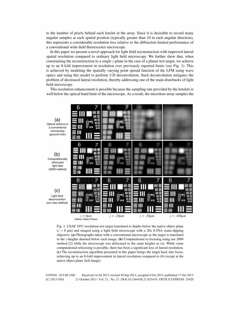


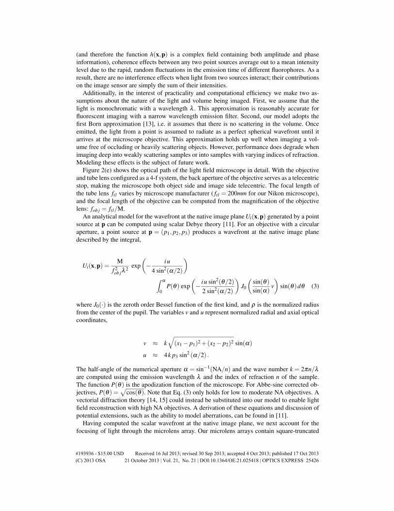


![Blind Deconvolution of Widefield Fluorescence Microscopic ... · eral deconvolution methods in widefield microscopy. In [3] several nonlinear deconvolution methods as the Lucy-Richardson](https://static.documents.pub/doc/80x56/5f6dfa53e2931769252d0293/blind-deconvolution-of-widefield-fluorescence-microscopic-eral-deconvolution.jpg)