Coastal Imagery Analysis and Breaking Wave Type Estimation with Machine Learning

Jorge Arce-Garro∗1, Taewon Cho∗2, Hye Rin Lindsay Lee∗3,Ryleigh Moore∗4, Risa R. Sayre∗5, Yao Xuan∗6, Zitong Zhou∗7

Faculty Mentors: Matthew Farthing8, Tyler Hesser8, Harry Lee9

Abstract

Classifying and identifying ocean wave breaker types is important to guarantee the safety and success ofboth civilian and military operations occurring in and around the surfzone. Current high fidelity numericalmodels are sensitive to boundary conditions and are not fast enough to solve this problem in the time frameneeded. An empirical parameterization for wave breaking type is employed using offshore wave conditionsand surfzone slopes estimated from an inverse method using nearshore video imagery. Machine learningmodels are attractive due to their speed and ability to predict information using less information thanother methods. In this paper, a direct method is used to label training data for multiple machine learningapproaches in order to predict the wave breaker types given an image and offshore wave conditions.

1 Introduction

Estimating the coastal hydrodynamics and ocean conditions is important for both the safety and successof civil works and military missions of the United States armed forces. Military operations can require thetransport of people and equipment from deep water to the beach. However, the dynamics of waves in thenarrow strip between these two zones must be better understood in order to avoid navigational difficulties,damage to ships, and even deaths due to treacherous plunging waves. The main cause of this danger is theprocess of wave breaking, since this is the mechanism by which a wave can release energy on its surroundings[1]. Therefore, wave breaking must be analyzed first in order to provide recommendations or predictions toavoid this damage.

2 Objective

This study focuses on developing an algorithm to predict the type of breaking waves at a beach for a givenmoment in time; this will be done by using the most readily available nearshore wave conditions, imagery,and corresponding data for the wave height and period. Ultimately, this algorithm will be able to employforecasts of wave height and period data as well as an image of the beach to generate probabilistic forecastsof the breaking types.

* Denotes co-first authors listed in alphabetical order by last name.1Department of Mathematics, University of Michigan2Department of Mathematics, Virginia Tech3Department of Mathematics, Applied Mathematics and Statistics, Case Western Reserve University4Department of Mathematics, University of Utah5Department of Environmental Sciences and Engineering, University of North Carolina - Chapel Hill6Department of Mathematics, University of California - Santa Barbara7Department of Energy Resources Engineering, Stanford Universiy8United States Army Corps of Engineers, Engineer Reseach and Development Center (USACE, ERDC)9Department of Civil and Environmental Engineering, University of Hawai’i at Manoa

1

Figure 1: Wave Breaker Types at Duck, N.C. - Source: Brodie et al. (2018)

Table 1: Criteria for breaking wave classification, where I is the Iribarren number. - Source: Battjes et al.(1975)

Breaker type I range

Spilling I < 0.5Plunging 0.5 < I < 3.3Surging I > 3.3

2.1 Wave Breaking

As waves come from deep water to shore, forces from the seabed slow them down and reduce their wavelength.Conservation of energy flux requires their heights to increase, in a phenomenon known as shoaling [2]. Theshoaling process causes the top of the wave, the crest, to move faster than the bottom, the trough, whicheventually causes the crest to spill over and to break, releasing the potential energy that has built up fromthe slowing of the wave.

There are three main wave breaking types that are being considered in this research: spilling, plunging,and surging. The breaking types of waves are determined by the wave height, wave period, and the underwatertopography near the shore, or the bathymetry. (See Figure 1). In general, the spilling and collapsing wavesare considered safe for boats trying to cross the surfzone, the area where breaking waves are observed. On theother hand, plunging waves are the most dangerous for boats. Their steep crests plunge violently when theybreak, exerting a sudden force that can disrupt a boat’s path, or even capsize it.

2.2 Classification of Breaking Types

An approach found in the literature to classify breaker types is the Iribarren number [1]. Let m denote thebeach slope, and let Hd and Ld denote the height and wavelength of a wave in deep water, respectively. TheIribarren number at deep water is the dimensionless parameter defined by

I =m√Hd/Ld

. (1)

The criteria in Table 1 have been established for breaking wave classification empirically [3].The Table 1 and equation (1) are deduced from breaking waves using constant slopes. The actual beach

geometries differ significantly from the assumption of constant slopes, especially in the surfzone.

2

Figure 2: Comparing bathymetry approximations from varying methods [5]

2.3 Estimating Bathymetry

Calculation of the Iribarren number requires the bathymetry in order to estimate the slope. A first approx-imation can be given by an equilibrium beach profile, or Dean profile [4], which consists of a simple convexparametrization of the form h = Ay2/3, where h is the water depth, and y is the offshore distance. The flaw ofthis model is that it uses an unrealistic topography which does not take into account sand bars - modulationsin the sea bed usually caused when storm waves erode the shore and deposit sediment in intermediate (oftenbetween 2 and 6 meter) depths. For reference, see Figure 2. The sand bars are crucial components whenit comes to classifying breaking types, as they often provide the first line of breaking waves that shape thedimensions of the surfzone.

As an additional complication, bathymetry is dynamic; it is constantly changing due to wave interactionand sediment transport [6]. In order to account for quickly changing bathymetry, the interest in bathymetryestimations from remotely collected data has increased over the years. There are several techniques availablethat use aerial visual inputs such as video imagery [7], surfzone pictures [5, 8], and Light Detection and Range(LIDAR) measurements [9, 10]. The most easily obtainable source of aerial visual input are overhead picturesof the surfzone, which can be generated by a drone. This study uses the algorithm by Holman et al. [8] to usethis aerial imagery to identify the 2D coordinates of the shoreline and sand bar into a parametric estimationof the 2D bathymetry.

Once a bathymetry estimate is available, it must be noted that the slope in general is not constant overthe seafloor. It can be argued that the slope values near the breaking point, where the wave first breaks, arerelevant to the breaking process; therefore, one of these slope values should be picked and used in (1).

3 Approach

This report describes two approaches to solve the problem of classifying the breaker type. The first method isa direct approach resulting in an Iribarren number calculation, and the second approach is a machine learningmethod. This initial approach is able to predict the expected breaking wave types in its own right, and alsoit will be used to label the training data for the machine learning model with a breaker type. Subsections 3.1and 3.2 describe these 2 approaches and their differences.

3

Figure 3: Three types of wave images from an Argus monitoring system at Egmond aan Zee - Source: FlandersMarine Institute

The following data is used for both approaches:

• Imagery data: An Argus monitoring system was used to produced imagery data of the coastline nearthe USACE Field Research Facility (FRF) in Duck, NC. The Argus monitoring system was developedby Oregon State University’s Coastal Imaging Lab, and it uses six different cameras pointing at differentdirection to produce a 180◦ view of the coast. This system samples every half an hour to an hour all yearround and produces a number of imagery products, but for this project we will focus on two differenttypes of images: time exposure (TIMEX) and variance (VAR) images taken over 10 minute time spanwith a frequency of 2 Hz from 2015 to 2017 (See Figure 3).

• Offshore wave height (H) and period (T ) data: The wave heights and periods coming to shore vary atany given moment in time. The expected values, or averages, of these 2 physical quantities are collectedby an acoustic wave and current meter (AWAC) from sensors approximately 1 km offshore of Duck,NC. The significant wave height (Hs) is used as a proxy for offshore wave height, and the period isapproximated by the sea surface wave period at variance spectral density maximum (Tp). It is assumedthat these averages remain spatially constant along the entire beach. This is a reasonable assumption,as the coastline region under this study is relatively small at only 2 km in length.

In order to gather offshore information, the the AWAC takes samples over approximately 22 minuteintervals. Specifically, the significant wave height

Hs = 4√mo

is determined from the zeroth moment

m0 =

∫ ∞0

E(f)df

of the energy function, where f is the frequency, and E is the energy. The zeroth moment is the totalarea under the wave energy density spectrum [11]. For the wave length, the value

Tp =1

fo,

where fo is the frequency associated with the highest amplitude of the wave energy spectrum [11].

Finally, the offshore wave length L is calculated using the dispersion relationship

σ2 = gκ tanh(κh). (2)

.

4

Figure 4: Flowchart of the direct approach

5

Figure 5: The examples of unsuitable images. Each image is labeled according to the type. From left to right,they correlate to the image requirements list starting from number 2.

3.1 Direct Approach

The Figure 4 outlines the flow of the first approach.

First, the TIMEX and VAR images of the surfzone are input into an image processing tool to identify theshoreline and sand bar locations. These locations are passed into a tool (described below in step 2 of thisapproach) that solves an inverse problem to calculate the bathymetry of the beach. Finally, the bathymetry isused to approximate a slope at the breaking point and offshore wave conditions in order to classify the wavetype using the Iribarren number.

Step 1: Image Data Cleaning and Processing

Approximately 6000 TIMEX and VAR images ranging from 2015 to 2017 were downloaded from the OregonState University Coastal Image Lab. Unfortunately, not all the downloaded images were suitable for thepurpose of this study. The requirements of the image data are:

1. Both TIMEX and VAR images must be available at the same time and day.

2. The entire range of image must be present.

3. There must be distinct evidence of wave breaking in the image.

4. The TIMEX images cannot have glares.

5. The VAR images must have a black shore.

6. There should not be any light beam pattern in the image.

Most of the suitable images were from the months of January through May and December, and the besttimes to sample the images were from 10 am to 4 pm EDT (see Figure 6). In general, the images fromJune through November usually did not contain any breaking waves or had too much noise, and the imagesfrom outside of the peak sample time range were usually too dark or bright to process. Out of about 6000downloaded images, only 644 images met the requirements above. Recall that both TIMEX and VAR imageswere being used to extract the shorelines and breaking points, which yields a total of 322 images of usable

6

Figure 6: Example dataset of image counts used for model training by month and year. No images from Julyor August were selected in the set.

data with RemoveSingle.m, RemoveGlare.m, and RemoveCameraDead.m. Some unsuitable images were ableto be screened. However, not all images were screened automatically because each case has different patternin its image while the others are hard to extract their pattern numerically.

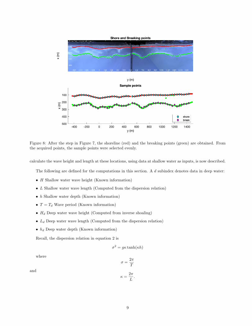
From the suitable images, the coordinates of the shoreline and breaking point need to be extracted in orderto estimate bathymetries. This can be done by detecting the two local maxima of the intensity per column ofthe gray-scaled TIMEX or VAR image. The algorithm is described below in Algorithm 1.

Algorithm 1 Detecting shore line and breaking points from a pair of TIMEX and VAR images (292× 1263)

1: for y=1:1:1263 dodz(x) = zV (x+ 1, y)− zV (x, y)xs = arg max

τs≥xdz(x)

z(x, y) = min(zT (x, y),zV (x, y))Solve Eq.(3)

2: end for

The images are first converted to gray-scale for low cost computation from RGB type, then they arecropped to remove labels and missing pixels. Let x be vertical coordinate from the top in an image and thehorizontal coordinate of the searching slide where the bar goes from left to right to search (the second plotof Figure 7), y be the horizontal coordinate of shoreline and bar in an image, and zT , zV be the intensities ofthe TIMEX and VAR images, respectively. After cleaning the images further, the coordinates of the shorelineand sand bar, y, are found by browsing slide intensity function values, zT and zV with respect to x. SinceVAR images have zero intensity, zV , above the shoreline (upper white region), those areas should be pitchblack. The coordinates of the shoreline is obtained when the intensity of VAR image reaches its first maximumdifference in intensity (See Algorithm 1); this happens at the white area in the VAR image. Note that x goesfrom top to bottom of the VAR image, however this does not work when the VAR image has noise. Findingthe breaking point coordinates is more challenging than the shore line coordinates as there are likely to bemore than one local maximum intensity after shoreline. Normally, the outer bottom edge of white lower regionis estimated as the breaking points, because the foam starts emerging from the breaking points which appears

7

Figure 7: The top figure shows gray-scale image and shore (red) and breaking point (green) column-wise. Thebottom plot shows the slide of VAR image and slide of min(TIMEX,VAR) along the red vertical line in the topfigure.

in white as well. Consider the following objective function to obtain the most appropriate breaking point byadding a penalty term and modifying the area of trapezoid,

xb = arg maxx≥xs

(z(x, yb) + z(xs, ys)

2

)log(x) + log

(x− xs

75

)(3)

where yb = ys in the same column, z = min(zT (x, y), zV (x, y)), (xs, ys) is the shoreline coordinate, (xb, yb) isbreaking point coordinate, and z is the intensity defined in Algorithm 1 (see Figure 7).

Step 2: Bathymetry and Slope Estimation

Recall that using the Iribarren number requires knowing the beach slope, m. There is a parametric beachtool, provided by USACE, that finds the 2D bathymetry based on the work of Holman et al. [8].

Using this, the bathymetry is estimated by sampling 49 1D cuts along the seaward direction of each image.These cuts allow to account for changes in the bathymetry along the coastline in a simple way. Figure 9illustrates several of these bathymetry profiles.

The slope is calculated right before the breaking point and then used in Iribarren’s formula. Specifically,the maximum slope over an interval of 100 meters prior to the breaking point is selected as the slope of eachbathymetry profile.

Step 3: Inverse Shoaling and Dispersion Relation

Although the wave height and period data at shallow water (from between 6 and 11 meters in depth) is avail-able, the wave information at deep water is the actual data required as an input for (1). Henceforth, the wavedata measured at the water depths of 100 meters or more will be considered as deep water. A procedure to

8

Figure 8: After the step in Figure 7, the shoreline (red) and the breaking points (green) are obtained. Fromthe acquired points, the sample points were selected evenly.

calculate the wave height and length at these locations, using data at shallow water as inputs, is now described.

The following are defined for the computations in this section. A d subindex denotes data in deep water:

• H Shallow water wave height (Known information)

• L Shallow water wave length (Computed from the dispersion relation)

• h Shallow water depth (Known information)

• T = Td Wave period (Known information)

• Hd Deep water wave height (Computed from inverse shoaling)

• Ld Deep water wave length (Computed from the dispersion relation)

• hd Deep water depth (Known information)

Recall, the dispersion relation in equation 2 is

σ2 = gκ tanh(κh)

where

σ =2π

T

and

κ =2π

L.

9

Figure 9: Bathymetry examples with varying distances from shore.

10

First, we can find L and Ld using the dispersion relation. Below is the explanation to find Ld. Thecomputation for L is similar. (

2π

Td

)2

= g

(2π

Ld

)tanh

(2π

Ldhd

)

Using linear wave theory, it is assumed that the period is constant, [11] hence T = Td(2π

T

)2

= g

(2π

Ld

)tanh

(2π

Ldhd

).

When hd is known, the only unknown in the equation is Ld, which can be solved by using any numericalmethod for nonlinear equations. In this work, an initial guess using the deep water approximation of

Ld ≈g

2πT 2d , (4)

was used. Notice that this approximation is the large limit of the dispersion relation (see equation 2) ash→∞.

Now to find Hd, the conservation of energy flux [2] requires

dECgdx

= 0, (5)

whereE = ρgH2/8

is the wave energy, ρ is density, cg is the group celerity, and g is the acceleration due to gravity.From this conservation law,

ECg = EdCgd

⇒ 1

8ρgH2Cg =

1

8ρgH2

dCgd

⇒ H2 1

2

L

T

(1 +

4πhL

sinh( 4πhL )

)= H2

d

1

2

LdTd

(1 +

4πhdLd

sinh( 4πhdLd

)

)

⇒ Hd =

[H2 12LT

(1 +

4πhL

sinh( 4πhL )

)12LdTd

(1 +

4πhdLd

sinh(4πhdLd

)

) ]1/2

⇒ Hd =

[H2L

(1 +

4πhL

sinh( 4πhL )

)Ld

(1 +

4πhdLd

sinh(4πhdLd

)

) ]1/2,

which can be directly computed. Above, the group celerity

Cg =1

2

L

T

[1 +

4πhL

sinh( 4πhL )

]was used as well as T = Td from linear wave theory [11].

11

Without Spilling Slope Plunging Slope Surging SlopeInverse Shoaling (Degrees) (Degrees) (Degrees)

Min [0, 0.98) [0.98, 6.45) [6.45, 90)Max [0, 7.48) [7.48, 40.91) [40.91, 90)

Average [0, 3.19) [3.19, 20.22) [20.22, 90)

Table 2: Estimated slopes needed for each wave breaker type based off of 19,525 wave data collections atDuck, NC from 2015-2018.

With Spilling Slope Plunging Slope Surging SlopeInverse Shoaling (Degrees) (Degrees) (Degrees)

Min [0, 0.52) [0.52, 3.44) [3.44, 90)Max [0, 7.29) [7.29, 40.16) [40.16, 90)

Average [0, 2.82) [2.82, 18.03) [18.03, 90)

3.1.1 Inverse Shoaling vs. Non-Inverse Shoaling Analysis - To Inverse Shoal or Not to InverseShoal

In Duck, NC, a research is being conducted to collect data in order to better understand the ocean wave dy-namics. In this section, the results of offshore data from 2015-2018 are examined in order to better understandthe behavior and distributions of offshore wave height, Ho and offshore wave length, Lo. Since these valuesare used to calculate the Iribarren number, Lo and Ho information provides a way to analyze the bathymetrynecessary to create each wave type (see table 1).As waves get closer to shore, they are affected by a process called shoaling. Shoaling occurs when waves “feel”the ocean floor and begin to grow in height. As a result of the conservation of wave energy flux and the disper-sion relation (equation 4), they develop a smaller wavelength while they change in height. Shoaling providesa more accurate way to compute Lo than using the deep water approximation to the dispersion relation.

Note that the data collected was waveTp (Peak Spectral Period) and waveHs (Significant Wave Height)from an 11m AWAC sensor. In order to gather offshore information, the the AWAC takes samples overapproximately 22 minute intervals.

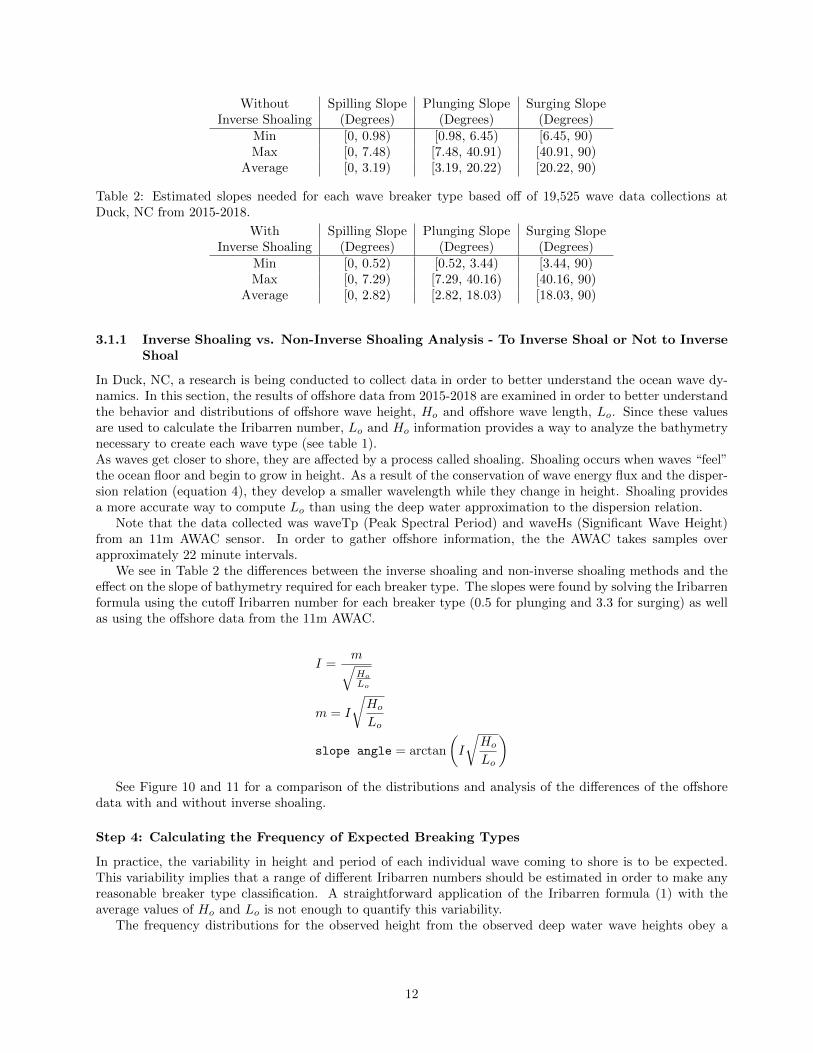
We see in Table 2 the differences between the inverse shoaling and non-inverse shoaling methods and theeffect on the slope of bathymetry required for each breaker type. The slopes were found by solving the Iribarrenformula using the cutoff Iribarren number for each breaker type (0.5 for plunging and 3.3 for surging) as wellas using the offshore data from the 11m AWAC.

I =m√HoLo

m = I

√Ho

Lo

slope angle = arctan

(I

√Ho

Lo

)See Figure 10 and 11 for a comparison of the distributions and analysis of the differences of the offshore

data with and without inverse shoaling.

Step 4: Calculating the Frequency of Expected Breaking Types

In practice, the variability in height and period of each individual wave coming to shore is to be expected.This variability implies that a range of different Iribarren numbers should be estimated in order to make anyreasonable breaker type classification. A straightforward application of the Iribarren formula (1) with theaverage values of Ho and Lo is not enough to quantify this variability.

The frequency distributions for the observed height from the observed deep water wave heights obey a

12

Figure 10: Distributions of offshore data Lo, Ho, and√

HoLo

respectively using 19,525 data points. The blue bars

represent the probability distribution without inverse shoaling, and the transparent orange bars represent thesame but with inverse shoaling. The brown region is the overlapping area between two probability distributions.

13

Figure 11: Difference graphs of wave characteristics used in the Iribarren calculations. The shoaling affectsthe wave length, wave period, and the denominator of the Iribarren formula.

14

Figure 12: Data from Oct 25 at Duck, NC over the course of 24 hours from different AWAC monitor depths.

15

Figure 13: Heatmap showing the correlation between 12,131 rows of data used to train and test the model.

Rayleigh distribution with density function [1, 12],

f(x;σ) =x

σ2e−

x2

2σ2

which can be entirely characterized by its mean. The Iribarren number calculations for this study do notintroduce variance for this quantity as no reference to a frequency distribution is available. Due to this,the inverse shoaling procedure is used to calculate the wave height average at deep water, and this value isused as the mean of the wave height distribution. A Monte Carlo simulation is followed by picking 10,000random height values based on this distribution, and as a result, 10,000 Iribarren numbers are correspondinglycalculated. The Table 1 is used again to classify these numbers, and then, the percentages of each expectedbreaking type are calculated. These calculated percentages are interpreted as the probabilities of observingeach breaking type along each 1D bathymetry strip.

3.2 Machine Learning Approaches

As described above, the direct approach of breaker type classification requires imagery data pre-processing,the bathymetry and its slope estimation, inverse shoaling for the deep water wave properties with MonteCarlo simulation, and calculation of the Iribarren number. To gain higher computational efficiency andmore knowledge on the relationship between the imagery data and the breaker types, the machine learningapproaches to classify wave breaker types based on breaking points were explored. The wave breaker typein the direct approach is uniquely determined by the bathymetry and offshore wave height and wave length.Moreover, the bathymetry is simulated with the coordinates of the breaking points and shoreline. Therefore,these coordinates together with the offshore wave conditions are sufficient to determine the wave breaker type.Based on this, a machine learning approach is proposed and tested to accelerate the direct method.

In this machine learning approach, the imagery data is pre-processed to identify the breaking points andshoreline coordinates. Then, the offshore wave height and period information will be collected and processed

16

Figure 14: Machine Learning step of the study. This follows from Figure 4.

by the inverse shoaling to get the deep water wave height and length. With these inputs, a surrogate modelwill obtain the the probability of each breaker type. The processes avoided by the this machine learningapproach are shown in Figure 14.

Note that the breaker type is obtained for each cut of the image as mentioned in section 3.1. Each cutof the image corresponds to one set of breaking point and shoreline coordinates {xb, xs, yb, ys(yb = ys)}. Thedirect method used to classify breaker type depends on the local bathymetry. The reason behind cutting theimages into 1D strips and predicting the label of each cut is that the bathymetry of each strip is calculatedlocally. Although there is correlation of bathymetry in the whole image, the further from the cut, the lowerinfluence gets when determining the bathymetry at a certain cut.

The 49 1D cuts correspond to 49 sets of breaking and shoreline coordinates. To include some spatialcorrelation, the coordinates of these cuts’ two closest neighbours are also included as the input of the surrogatemodel for the prediction of the breaker type at each cut. The output of the model then consists of three valuescorresponding to the probability of each breaker type. An illustration is shown in the Figure 15. From thestrips of 322 images, 12,138 samples are obtained after some data cleaning.

To obtain this surrogate model, Neural Networks, Support Vector Machine Regression, and Random ForestRegression are explored.

3.2.1 Neural Networks

Neural Networks were tried as the first surrogate modeling approach for their capability to perform regressiontasks. The data set was split into training, validation, and testing sets by the following ratio: (70%, 15%, 15%).

Shown in the Figure 16, the architecture of the best performed Neural Network consists of 2 linear affinelayers, where each linear layer is activated by a ReLU activation layer.

Mean square error loss function is used to compare the prediction with the targets.At the training stage, a L2 norm regularization term of the Neural Network parameters is added to the loss

function to prevent overfitting. The Neural Network was then trained to minimize the loss over the trainingset. The validation set is used to check the performance of the Neural Network with the mean square error.The best performing Neural Network obtained in this project used SGD optimizer [13], and it has the followingstructure and hyper parameters:

Learning rate: 0.001

regularization weight: 0.001

Optimizer: SGD

Input: 11

Linear Layer: 20 units, ReLU

Linear Layer: 40 units, ReLU

Output: 3

17

Figure 15: Input and output of the surrogate model

Figure 16: Neural network architecture

18

Figure 17: Single Decision Tree Figure 18: Random Forest with n Decision Trees

This Neural Network was trained for 1000 epochs to reach the best performance. Google Colab was used forthe training with its GPU resource to accelerate the gradient descent, and the training was done in 219.10s.

3.2.2 Random Forest Regression

Random Forest is an ensemble learning method based on decision trees. Decision trees are classification andregression models in the form of tree structure. In each decision tree, there are decision nodes and leaf nodes,and each decision node is connected to two or more leaf nodes. Data space is partitioned into several subspacebased on the similarities of features. The similarities and partition depends on the metric in feature space.Gini impurity and information gain are widely used metrics. When an observation is put in the tree, startingfrom the root decision node, it will go through several decision nodes and finally fall into the region where mostobservations have similar features with it. The prediction result of each observation depends on the fittingresults of other observations in the region. More details of decision tree could be found in [14]. Sometimessingle decision tree does not work very well due to overfitting and corresponding high variance. Random Forestcorrects the decision trees by ensembling several decision trees together. Given a dataset {Xi}, {1 ≤ i ≤ N}with corresponding responses {Yi}, n random subsets are taken with replacement. Decision trees are builton these subsets separately with random chosen features. Suppose that test observation is X, predictions ondecision tree j is dj(X), then the prediction result of random forest is

f(X) =1

n

n∑j=1

dj(X);

which lead to better performance by decreasing the variance of the system. Random Forest regression is usedto predict the probability of different wave breaker types. The input and output are the same as the ones inthe Neural Network. The only difference is that three random forests are built to predict the probability of thespilling, plunging, and surging waves, and the predictions are normalized to ensure that the sum of predictedprobabilities sum to 1.

19

3.2.3 Nonlinear Support Vector Machine Regression

More machine learning approaches are implemented on the same training set. Support Vector Machine Re-gression (SVR) is a basic machine learning approach for the classification and regression as well. As mentionedin the previous sections, the prediction of probability of different breaker type (spilling, plunging, surging) canbe seen as three regression problems. Nonlinear Support Vector Machine could be applied to these problemsby transforming input into high dimensional Hilbert space and fitting the function in this space. Given atraining set {Xi}, 1 ≤ i ≤ N and corresponding respfonses {Yi}, Support Vector Machine Regression (SVR)is in the form of [15]

f(x) =

N∑i=1

(an − a∗n)G(xn, x) + b

where a = (a1, ...an) is the saddle point which minimizes

L(a) =1

2

N∑i=1

N∑j=1

(ai − a∗i )(aj − a∗j )G(xi, xj) + ε

N∑i=1

(αi + α∗i )−N∑i=1

yi(ai − a∗i )

subject toN∑i=1

(ai − a∗) = 0

∀i, 0 ≤ ai ≤ C

∀i, 0 ≤ a∗i ≤ C.

G(, ) is the kernel function, which has multiple choices, like radial basis function Kernel and polynomial kernel.In this project, the radial basis kernel defined by

G(x,y) = exp(−γ‖x− x′‖)

and is used for SVR regression. In SVR regression, the radial basis function kernel decreases the weights ofpoints that are far away from the predicting point, which make the predicted function value of given point closeto the values of its neighbors in the Hilbert space. Maps from the local window of stripes to the probabilityof three types of waves are predicted by three separate SVR systems. The inputs and outputs are the sameas what is defined on Figure 15.

4 Evaluation Experiments

The work of Brodie et al. contains 5 different frequency observations for the percentage of breaking and non-breaking waves measured at Duck, NC, on October 25th, 2017 between 1 and 4 pm [16]. These observationsallow for the following experiments.

1. Evaluation of the machine learning algorithm compared to the direct approach: Predictionsfor beach profiles image and Ho and To data corresponding to the times and date described above willbe calculated via the direct approach and the machine learning approach. These predictions will thenbe compared.

2. Comparing estimated and observed breaking wave type frequencies: On October 25th, 2017,the proportion of spilling and plunging breaking waves were manually classified at five time points for asingle location at Duck, NC. Predicted breaking types from the direct approach, the machine learningmodel will be compared with these observations.

3. Bathymetry estimate validation: During October 2015, a bathymetry survey was completed byboat once each week. Image files were available within 12 hours of each reported bathymetry collection.Bathymetry calculated using the parametric beach model on a 141 by 107 grid will be validated againstcontours based on the interpolated results of this survey.

20

Figure 19: In the upper left, the yellow triangles represent the y-location where the bathymetry and breakingtype observations described below were collected. The upper right shows the times at which the observationsoccurred, and the offshore conditions during that day. The lower part of the figure represents the observedproportions of spilling and plunging waves at each time point (and similar spatial points) [16]

5 Results

5.1 Comparison of Observed Breaking Types and Estimated Breaking Types

On October 25, 2017, the direct observations of wave types at a position indicated by the yellow triangle inthe figure below were measured at five different time points (see Figure 19).

Estimations of bathymetry using Argus imagery from 13.5 hours before and 6.1 hours after these observa-tions were used to estimate breaking types near this spatial point (see Figure 20).

The calculated breaking types based on estimated bathymetry was compared to the manual classifications.About half of the observed waves were plunging and half were spilling during these time periods. Estimatesof the probability of plunging are calculated at about 20 m intervals along the shore (see Figure 21).

5.2 Comparison of Observed Bathymetry with Parametric Beach Model Result

Observed seabed measurements obtained in October 2015 provide the chance to evaluate bathymetry dataproduced by the parametric beach model. The comparison between aerial images taken within 12 hours ofthe reported survey time is shown. These images were not deemed suitable for the described image processingmethod, so the inputs to the parametric beach model were not available, and the calculated topography couldnot be compared (see Figure 22).

21

Figure 20: Comparison of predicted and observed [16] bathymetry for Duck NC, October 25, 2017. Thesandbar is closer to the shoreline in the estimated instantiation, and the slope from the shore is much steeper.The sandbar is less pronounced in the estimate. However, the results are qualitatively similar.

Figure 21: The estimated probabilities of plunging at five intervals around and including the observations ofbreaking types. The top estimate (which is prior to the known data) is showing a probability of plungingwhile the bottom estimate (which is after the known data) shows almost no chance of plunging.

Figure 22: Contour representing the results of bathymetry survey for October 2015 superimposed on Argusimage data from within 12 hours of the survey. The title of each image represents the Unix time in GMT.

22

Figure 23: Support Vector Machine Regression Figure 24: Random Forest

5.3 Machine Learning Surrogate Model Performance

To evaluate the performance of the machine learning approaches, prediction of the breaker types on onetraining data and one test imagery data were produced and shown in Figure 26 and 27. The near shore areawas segmented into 49 strips in each image, for each of these strip, a breaker type is predicted. Comparisonsbetween the results of the direct model and multiple machine learning approaches are shown. The colorintensity indicates the probability of the existence of plunging wave on the corresponding strip. An overlap ofthe image with the breaker type prediction is shown in Figure 28 to illustrate.

5.3.1 Neural Networks

With the data set and architecture described in section 3.2.1, the training and validation loss curve of theNeural Network is shown in Figure 25. Although the training and validation loss seem to decrease to a lowlevel, the performance of each prediction task was not as good as that of SVR. The visualization of theprediction on two days is shown in the evaluation section together with that of other surrogate models inFigure 26 and Figure 27. Figure 26 is in the training set and Figure 27 is in the testing set. Note that theprediction at the center of the Figure 26 diverged from the direct method, one possible reason may be theappearance of the pier in the center of the image, and the Neural Network was not able to handle this noise.Further more, the overall performance of the Neural Networks was worse than the random forest and SVR,the reason for this might be the scarcity of training data, the difficulty to tune the hyper parameters, and thechoosing of the loss function.

5.3.2 SVR and Random Forest

The training of SVR and Random Forest is efficient. Mean square error bar on test sets (1821 observations)is shown in 5.3.2. Considering the short training time, the result of both methods are encouraging. Thecomparison of physical model and machine learning methods are shown in Figure 26 and Figure 27.

5.3.3 Modeling Time Comparison

Comparison of modeling time of the two imagery data is shown in table 5.3.3. SVR outpermed all the othermethods in terms of modeling time and the accuracy.

Method Direct Approach Random Forest Support Vector Machine Regression Neural NetworkTime(s) 675.48838 0.00671 0.00960 0.02911

Table 3: Modeling time for 2 imagery predictions

23

Figure 25: Training and validation loss

Figure 26: The comparison between the result of training data of direct approach, Support Vector MachineRegression, Random Forest, and Neural Network from top to bottom respectively, using the same image.Darker red represents higher probability of plunging waves in that region.

24

Figure 27: The comparison between the result of test data of direct approach, Support Vector MachineRegression, Random Forest, and Neural Network from top to bottom respectively, using the same image.Darker red represents higher probability of plunging waves in that region.

Figure 28: Example of result visualization for a day at Duck, NC. The darker the red, the greater theprobability of plunging waves occurring.

25

6 Conclusions and Future Work

In this report, a breaker type classification tool based on the imagery data and offshore wave information isproposed and tested. Note that this task has not been done in the past. The direct method described insection 3.1 receives an imagery of the near shore area, simulates the bathymetry, computes the slope of theseabed at the breaking point, then classifies the breaker type with Iribarren number classifier.

Moreover, to simplify the direct method and reduce computational cost, several machine learning methodswere explored. The Figure 26 and 27 show the probability of plunging at a region of image using all themethods in this study. It is clearly shown that the direct approach, SVR regression, and Random Forest yieldssimilar results in two images. Among Neural Networks, Support Vector Machine regression, and RandomForest, the most robust and well performed model is the SVR.

There are few ideas that could be explored if given more time. First, a probability distribution was usedfor Ho but not for To, and the distribution of To was not found in the literature. If given more time, themore research and study could be done to find this distribution. Second, there were some issues with theimage processing. The unsuitable images are manually and automatically discarded. The screening processwas available in the cases of an image missing chunks of a region, not having both of TIMEX and VARimages, and glares in an image. However, the cases of not having a distinct evidence of wave breaking, VARimage’s shore not being pitch black, and any light beam pattern present in the image were not able to screenautomatically. Convolution or filtering methods are needed to detect their patterns in the images. Third,the result visualization could be automated to overlay images for the final output. Lastly, more labeled andimagery data are needed to classify the breaking types better.

References

[1] H. N. Southgate, “Wave breaking-a review of techniques for calculating energy losses in breaking waves,”1988.

[2] M. R. Gourlay, Wave Shoaling and Refraction, pp. 1149–1154. Dordrecht: Springer Netherlands, 2011.

[3] J. A. Battjes, “Surf similarity,” in Coastal Engineering 1974, pp. 466–480, 1975.

[4] R. G. Dean, “Equilibrium beach profiles: characteristics and applications,” Journal of coastal research,pp. 53–84, 1991.

[5] R. A. Holman, D. M. Lalejini, K. Edwards, and J. Veeramony, “A parametric model for barred equilibriumbeach profiles,” Coastal Engineering, vol. 90, pp. 85–94, 2014.

[6] H. Ghorbanidehno, J. Lee, M. Farthing, T. Hesser, P. K. Kitanidis, and E. F. Darve, “Novel data assim-ilation algorithm for nearshore bathymetry,” Journal of Atmospheric and Oceanic Technology, vol. 36,no. 4, pp. 699–715, 2019.

[7] K. L. Brodie, M. L. Palmsten, T. J. Hesser, P. J. Dickhudt, B. Raubenheimer, H. Ladner, and S. Elgar,“Evaluation of video-based linear depth inversion performance and applications using altimeters andhydrographic surveys in a wide range of environmental conditions,” Coastal Engineering, vol. 136, pp. 147–160, 2018.

[8] R. A. Holman, D. M. Lalejini, and T. Holland, “A parametric model for barred equilibrium beach profiles:Two-dimensional implementation,” Coastal Engineering, vol. 117, pp. 166–175, 2016.

[9] J. L. Irish and T. White, “Coastal engineering applications of high-resolution lidar bathymetry,” Coastalengineering, vol. 35, no. 1-2, pp. 47–71, 1998.

[10] V. Ramnath, V. Feygels, H. Kalluri, and B. Smith, “Czmil (coastal zone mapping and imaging lidar)bathymetric performance in diverse littoral zones,” in OCEANS 2015-MTS/IEEE Washington, pp. 1–10,IEEE, 2015.

[11] R. Dean and R. Dalrymple, Water Wave Mechanics for Engineers and Scientists. Englewood Cliffs, N.J.:Prentice-Hall, 1984.

26

[12] E. B. Thornton and R. Guza, “Transformation of wave height distribution,” Journal of GeophysicalResearch, 1983.

[13] H. Robbins and S. Monro, “A stochastic approximation method,” The annals of mathematical statistics,pp. 400–407, 1951.

[14] W.-Y. Loh, “Classification and regression trees,” Wiley Interdisciplinary Reviews: Data Mining andKnowledge Discovery, vol. 1, no. 1, pp. 14–23, 2011.

[15] “Understanding support vector machine regression.” https://www.mathworks.com/help/stats/

understanding-support-vector-machine-regression.html. Accessed: 2019-07-24.

[16] K. L. Brodie, A. Albright, P. J. Hartzell, S. Bak, C. O. Collins III, T. Hesser, and P. Dickhudt, “Multi-beam lidar observations of breaking waves,” in AGU Fall Meeting Abstracts, 2018.

[17] “The coastal imaging lab web.” http://cil-www.coas.oregonstate.edu. Accessed: 2019-07-20.

27