Wave slope and wave age effects in measurements of

electromagnetic bias

W. Kendall Melville, Francis C. Felizardo,1 and Peter MatusovScripps Institution of Oceanography, University of California, San Diego, La Jolla, California, USA

Received 10 November 2002; revised 30 November 2003; accepted 20 January 2004; published 27 July 2004.

[1] We present measurements of Ku band electromagnetic (EM) bias made for 2 monthsfrom a platform in Bass Strait off the southeast coast of Australia during the austral winterof 1992. EM bias, �, the difference between the electromagnetic and true mean sea levels,was measured using Doppler scatterometers. Linear wave theory was used to relate theDoppler signal to the surface displacement, giving simultaneous coincident backscatterand wave measurements, including significant wave height, Hs. On the basis ofdimensional reasoning, we suggest that the usual inhomogeneous correlations of thenormalized bias b = �/Hs with the 10 m wind speed, U10, and Hs may be improved bycorrelating the data with nondimensional variables, including a characteristic wave slope,s, and wave age, c/U10, where c is a characteristic phase speed of the surface waves. Usingboth polynomial correlations and optimal estimation techniques to fit the data, we find thatthe standard error of the fit is reduced by �50% when the dimensionless variables areused. We find that the dependence of the EM bias on the wave slope is consistent withearlier tower-based measurements and the theory of short-wave modulation by longerwaves. We discuss the implications of these results for operational implementation of EMbias algorithms based on wave slope and wave age. INDEX TERMS: 4275 Oceanography:

General: Remote sensing and electromagnetic processes (0689); 4594 Oceanography: Physical: Instruments

and techniques; 6969 Radio Science: Remote sensing; KEYWORDS: EM bias, radar altimetry, remote sensing

Citation: Melville, W. K., F. C. Felizardo, and P. Matusov (2004), Wave slope and wave age effects in measurements of

electromagnetic bias, J. Geophys. Res., 109, C07018, doi:10.1029/2002JC001708.

1. Introduction

[2] Electromagnetic (EM) bias remains one of the larg-est errors in radar altimetry for oceanographic applications.It results from the fact that, on average, the troughs of thesurface waves are better reflectors of radio waves than arethe crests, resulting in the electromagnetic mean sea levelbeing lower than the true mean sea level. This difference isknown as the EM bias. It was first discovered in tower-based measurements by Yaplee et al. [1971], and subse-quent tower [Melville et al., 1991; Arnold et al., 1995]and aircraft [Walsh et al., 1991; Hevizi et al., 1993]measurements have confirmed the effect and correlatedthe bias, �, with the wind speed, U10, and significantwave height, Hs . Attempts have also been made to inferthe EM bias from the altimeter data itself, by makingcertain hypotheses about the variability of the oceanbetween overflights [Chelton, 1994; Gaspar et al., 1994].In general, the aircraft and space-based results have led toestimates of the normalized bias, b = �/Hs, that are lessthan the tower-based measurements; however, Gaspar andFlorens [1998] have recently revised their earlier nonpara-

metric estimates of the bias, to give improved agreementwith the tower-based measurements.[3] A fundamental criticism of earlier attempts to corre-

late EM bias with wind and wave variables is that theresulting relationships have been inhomogeneous, givingthe dimensionless bias, b, in terms of the dimensionalsignificant wave height, Hs, and the dimensional windspeed, U10. The pragmatic reason for the use of thesecorrelations is that both the wave height and the windspeed can be inferred from the altimeter measurements,and if accurate, the correlations would make the altimetera ‘‘self-contained’’ instrument, not dependent on externalmeasurements for EM bias corrections. However, as newuses of altimetry demand greater accuracy, it may be thatthis outweighs the convenience of a self-contained systemfor EM bias, and supplementary measurements becomenecessary.[4] It is instructive to consider the problem in the context

of simple dimensional analysis. Let us assume that the EMbias, �, is dependent on the small-scale roughness of theocean surface, which is mainly a function of both the windspeed, U10, (as is assumed in scatterometry) and thestructure of the ocean surface at the scale of the longerwind waves and swell. The small-scale roughness may bemodulated by the longer waves, or the direct nonlineareffects of the longer wind waves may be significant. Ineither case, we assume that the longer surface waves can be

JOURNAL OF GEOPHYSICAL RESEARCH, VOL. 109, C07018, doi:10.1029/2002JC001708, 2004

1Now at Union Cement Corporation, Makati City, Philippines.

Copyright 2004 by the American Geophysical Union.0148-0227/04/2002JC001708

C07018 1 of 15

represented by a characteristic amplitude, al = Hs/2, say, anda characteristic wave number, kl, and radian frequency, wl.In mixed wind seas and swell, the slope of the swell isusually significantly less than that of the wind waves. TheEM bias is also a function of the wave number of the radiowaves, kr, but to include this effect the details of the small-scale roughness must also be represented [Arnold, 1992],and its representation by just U10 is inadequate. So, we limitourselves to considering the functional relationship for justone radio wavelength. Thus we have that

� ¼ � Hs;U10; kl;wl ; . . .ð Þ: ð1Þ

Now, by dimensional reasoning it follows that

b ¼ b Hsk;U10k=wl ; . . .ð Þ ð2Þ

or

b ¼ b alkl;U10=cl ; . . .ð Þ; ð3Þ

where alkl is a measure of the slope of the longer waves andU10/cl is the reciprocal of the wave age. One of the primaryaims of this paper then is to determine whether adimensionally homogeneous correlation of the dimension-less bias with the wave slope and wave age gives animprovement over the dimensionally inhomogeneous, butpragmatic correlations that have been used in the past.[5] The structure of the paper is as follows. In section 2

we describe the experimental site and the essential details ofthe measurements. In section 3 we present the techniques ofdata analysis and technical details of some of the measure-ments and calibrations, including the technique used toestimate a characteristic slope of the surface waves basedon the linear dispersion relationship and the measurementsof wave height. In section 4 we present the measurements ofEM bias over the course of the experiment, and show theusual correlations of EM bias with wind speed and waveheight. We also show the improved correlations of normal-ized EM bias with the wave slope and wave age, andpresent both polynomial fits and optimized empirical fitsto the data. In section 5 we review the major results of thepaper and discuss the implications of these results foroperational EM bias corrections.[6] Preliminary versions of this work have been pre-

sented as posters at the TOPEX/Poseidon Jason-1 ScienceWorking Team Meetings in 1998 and 1999 and at the Air-Sea Interface Symposium (Sydney, Australia) in 1999;they have also been posted on our Web site (http://airsea.sio.ucsd.edu). The data presented here have subse-quently been used in several studies that also address theuse of wave slope in describing EM bias using the datadescribed here. Millet et al. [2003a, 2003b], using thisBass Strait data supplemented by earlier tower data fromthe Gulf of Mexico [Arnold et al., 1995], show that theextended data set confirms the basic result of Melville etal. [1999] (see http://airsea.sio.ucsd.edu/Posters/EMBposter.pdf ) that the rms error in estimating bias is reduced by�50% when using wave slope instead of the usualparameterizations by wind speed and wave height. Milletet al. [2003a, 2003b] analyzed the two tower data sets andTOPEX/Poseidon data showing improved correlations

between models of bias based on the in situ data andthe satellite data. Gommenginger et al. [2003], using wavemodel (WAM) wave computations, show that the Srokosz[1986] model of sea-state bias leads to a quasi-linearrelationship between the sea-state bias coefficient and ther.m.s. slope of the longer gravity waves, and shows goodagreement with the tower data of Melville et al. [1991] andthe data reported here. They also found that the EM biaspredictions of the theory of Elfouhaily et al. [2000] weresensitive to the high-frequency tail of the surface wavefield. Most recently, Kumar et al. [2003] using an EM biasalgorithm inferred by the results presented here and thecurrent operational EM bias correction applied to TOPEX/Poseidon data, along with buoy measurements of windspeed and wave spectra and WAM wave modelling,conclude that EM bias corrections cannot be reliablyestimated from altimeter data alone, and will require inputfrom coupled ocean-atmosphere models, wave models andperhaps other satellite sensors.

2. Experiment Description

[7] An experiment to study the characteristics of electro-magnetic bias was conducted from 16 June to 26 September1992 (year day 167–325) on the Esso/BHP Snapper plat-form in Bass Strait, Australia. Two Ku band (14 GHz)coherent, continuous wave, dual-polarized scatterometersbuilt at the US Naval Research Laboratory (Washington,DC) were mounted at two different elevations at thesouthwest corner of the platform, which is in water 57 mdeep, 30 km offshore. Figure 1 shows a map of the locationof the experiment off the coast of southeastern Australia.[8] Figure 2 shows schematic diagrams of the platform

and the location of the different instruments, with thescatterometers (K15,K25) mounted 15 and 25 m, respec-tively, above the mean sea surface. When pointing at nadirthe footprints of the scatterometers at the sea surface were atleast 8 m away from the main legs of the platform, and inunimpeded wind and wave fields from the southwest half-plane. (It is well known that in storms the region immedi-ately around a platform may be foam covered due to wave/current/platform interaction. We have no relevant observa-tions of these effects for the Snapper platform and noaccount of foam coverage was taken in editing the data.)Both scatterometers were oriented toward nadir at the startof the experiment. The two-way half-power beam width ofboth scatterometers is 6.3�, giving 3 dB spot sizes at the seasurface of �1.7 and 2.7 m diameter for K15 and K25,respectively. The lower scatterometer was reoriented to a45� incidence angle on 19 August (year day 231) for adifferent study. We only present the measurements takenprior to that date.[9] The scatterometers were designed to generate a com-

plex valued output from the horizontally polarized (HH) andvertically polarized (VV) signals. The real and imaginarycomponents of the output were sampled at 3125 Hz by a12 bit analog-digital (A-D) converter mounted in a personalcomputer. A separate A-D converter in the same computerwas used to simultaneously sample, at 16 Hz, the data fromthree wire wave gauges and the anemometers. The othermeteorological instruments were polled every 10 min. Afterthe initial setup, the experiment ran independently until

C07018 MELVILLE ET AL.: MEASUREMENTS OF ELECTROMAGNETIC BIAS

2 of 15

C07018

Julian day 231, with the crew of the platform replacing theoptical storage disks every week.[10] Wind speed and direction measurements were made

at a 35 m elevation on the Snapper platform. Similarmeasurements were made at a 53 m elevation on KingfishB, a platform 45 km southeast of Snapper. The wind

direction sensor of the anemometer at the Snapper platformstopped working on 7 July (Julian day 188). Intercompar-ison of the anemometer data between the Snapper andKingfish B platforms prior to that date showed that forwinds coming from the southwest half-plane (135�–315�;see below) there was generally excellent agreement between

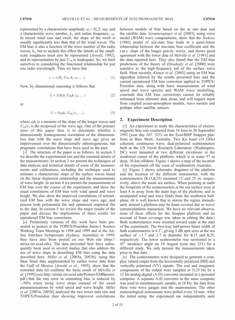
Figure 1. Location of the Esso/BHP Snapper and Kingfish B platforms in Bass Strait. The primarymeasurements were from Snapper, with some supporting meteorological measurements from Kingfish B.

Figure 2. Snapper platform and the location of the primary instruments. K15 and K25 are Ku bandDoppler scatterometers at 15 and 25 m above mean sea level (MSL), respectively. The wire wave gaugeswere separated by 1 m in orthogonal directions. The R. M. Young propeller anemometer was mounted35 m above MSL.

C07018 MELVILLE ET AL.: MEASUREMENTS OF ELECTROMAGNETIC BIAS

3 of 15

C07018

the wind directions at the two platforms which in a worstcase differed by at most 30�. Wind speeds from the samedirections were typically within ±1 m/s. This agreement isattributed primarily to the fact that winds in these directionswere either from the open sea at fetches much larger thanthe distance between the platforms or off a broad flat coastalplain. The wind direction data after 7 July were taken fromthe anemometer on the Kingfish B platform. The windspeed measurements were later reduced to the equivalentwind speed at 10 m elevation, U10, using an assumedlogarithmic wind speed profile [Wu, 1980; Smith, 1988]:

Uz � U zð Þ ¼u*k

lnz

z0; ð4Þ

with the roughness length, z0, given by

z0 ¼ zs þ zc ¼ 0:11n=u*þ 0:0185u*2=g; ð5Þ

where k = 0.4 is the von Karman constant, u* the frictionvelocity, n the kinematic viscosity of air, and g thegravitational acceleration. Thus we have two equations forthe two unknowns u* and z0.[11] Although instruments for measuring air temperature,

sea temperature and relative humidity were deployed at thestart of the experiment, the sea surface temperature andrelative humidity instruments stopped operating after a shortperiod of time. Hence we were unable to incorporate theeffects of atmospheric stability in computing the value forU10. Large and Pond’s [1981] results suggest that neglect-ing atmospheric stability will lead to an error of less than4% in U10.[12] Three nichrome resistance wire wave gauges were

installed on the platform in a triangular pattern near thescatterometer at the 15 m level (K15). The wires were �1 mapart along the orthogonal sides of the triangle and werecalibrated at the beginning of the experiment. This wasaccomplished by positioning the wires at various predeter-mined elevations and sampling the mean voltage overseveral minutes at each position. On 19 August (Julianday 231), the wires were again calibrated, cleaned andcalibrated again.

3. Data Editing and Processing

3.1. Overview

[13] Figure 3 shows time series of the 10 m wind speed,U10, and direction, qw, (direction from which the wind iscoming), the significant wave height, Hs, (from the K15Doppler scatterometer measurements; see below), and thephase speed c at the peak of the wind wave spectrum,during the 64 day observation period. The measured hourlyaveraged values of U10 range from 0.6 to 15.4 m/s. Windspeeds up to 20 m/s were observed, although these eventsdid not last more than 20 min.[14] Since the scatterometers and wave gauges were

positioned near the southwest corner of the platform, windand waves coming from directions close to azimuth qw =225� are subjected to the least interference from the plat-form. The limits of the half-plane of qw values within 225� ±90� are denoted in Figure 3b by the two dashed lines. Of the1539 available hourly averages, 814 (53%) are included

within this half-plane, for which the minimum fetch is 50 kmto the northwest, extending to �500 km to the southwestand essentially infinite fetch to the southeast.[15] The determination of the peak of the wind wave

spectrum is relatively unambiguous in a multimodal spec-trum but in unimodal spectra it is less clear. In analyzingthese data we have set c equal to the phase speed at the peakof unimodal spectra. In consequence of this, we expect to bemeasuring the phase speed of the swell at low wind speeds.The data in Figure 3d show that the largest phase speedswere �15 m/s, corresponding to a wavelength of �145 m.In a water depth of 57 m, the correction to the phase speedfor finite depth effects is less than 1% for waves of thislength. Thus we expect the kinematics of the wave field tocorrespond to deep water conditions.

3.2. Scatterometers

[16] The scatterometer output time series were processedin the time domain using the covariance processing tech-nique [Doviak and Zrnic, 1984]. Our implementation of thismethod follows closely the method described and used byJessup et al. [1991], which gives a direct estimate of thepower, mean frequency and bandwidth of the complexvalued time series for each polarization (HH, VV) every0.0625 s. They were then saved to optical disks every 10 mintogether with the meteorological data and the wire wavegauge data. Hourly averages of the time series were latercomputed and used in this study.[17] The scatterometers were calibrated immediately

before and after deployment by measuring the rms ampli-tude of the complex valued output voltage of each polari-zation of the scatterometer using a 15 cm aluminum sphereas a target. The procedure used is described in detail byJessup [1990]. The results show that the drift in thecalibration of both channels of the K25 scatterometer wasminimal. The same is true with the HH channel of K15although the drift was slightly larger in this case. Thecalibration of the K15 VV channel on the other handdiffered significantly before and after the experiment dueto damage to one of the wave guides. An inspection of thehourly averaged time series of the cross section, s0, showedthat this occurred on approximately day 200, 32 days afterthe start of the experiment. While adjusting the calibrationfactors for the VV channel to account for this would havebeen feasible, we decided to avoid using potentially unre-liable K15 VV data after that date.[18] In computing s0, we note that the value of the

normalized scatterometer varies with the target range Rand the illuminated area A. Since the presence of surfacewaves modifies the range to the sea surface, a correction tothe value of the measured cross section s0,meas needs to beapplied. The value of s0 is proportional to R�4 and to A. Onthe other hand, the illuminated area A is proportional to R2.Hence the net value of s0 varies as R

�2. The scatterometercross section s0 is related to the measured scatterometercross section s0,meas by

s0 ¼ KH � hð Þ2

H2s0;meas; ð6Þ

where K is a calibration factor, H is the height of thescatterometer above the mean sea level and h is the sea

C07018 MELVILLE ET AL.: MEASUREMENTS OF ELECTROMAGNETIC BIAS

4 of 15

C07018

surface displacement at the scatterometer footprint asmeasured by the scatterometer (see below).

3.3. Doppler Wave Gauge

[19] Since the wire wave gauges were located outside thefootprint of the two scatterometers, parameters such as EMbias which require sea surface measurements that arecoincident with the scatterometer footprint cannot be com-puted from wire wave gauge data. We instead use themeasured Doppler shift from both scatterometers to inferthe fluctuation of the sea surface elevation at the footprint ofboth scatterometers. This method was earlier used byArnold et al. [1995] and the errors are reviewed here.[20] The kinematics of the sea surface are described by

the free surface boundary condition

dhdt

¼ @h@t

þ u@h@x

þ v@h@y

¼ w; ð7Þ

where u = (u, v, w) is the velocity of the water at thesurface z = h. For slowly varying waves of small slope, i.e.,

alkl � 1, to leading order, the advective terms may beneglected, introducing an error of the order of (alkl):

w ¼ @h@t

1þ O alklð Þ½ : ð8Þ

The sea surface slopes over scales comparable to thefootprint of the scatterometers are typically in the rangeO(10�2–10�1).[21] An additional correction is required since the scatter-

ometer measures the Doppler shift due to the motion of thescatterers within the footprint. It is easy to show that thisleads to an error of O(cs/cl), where cs is the intrinsic phasespeed of the (unresolved) scatterers and cl is the phase speedof the longer (resolved) waves. We expect that for typicalconditions cs/cl � 1. The time series of the surface elevationcan then be well approximated by integrating the verticalvelocity, w, with respect to time.[22] The ability of this technique to resolve high-frequency

waves is limited by the size of the illuminated area, so

Figure 3. Time series of hourly averages of (a) the 10 m wind speed, U10, (b) the direction from whichthe wind was coming, qw, (c) the significant wave height, Hs, and (d) the phase speed at the peak of the(wind wave) spectrum (see text) for the duration of the experiment. The dashed lines at 135� and 315� inFigure 2b show the limits of the wind direction sector that was used to avoid interference from theplatform. Only data in this sector contributes to the final results in this paper.

C07018 MELVILLE ET AL.: MEASUREMENTS OF ELECTROMAGNETIC BIAS

5 of 15

C07018

that K15, which has a smaller footprint than K25, will be ableto resolve the smaller waves better than K25.We can estimatethe maximum frequency resolution of the two scatterometersusing the deep water dispersion relation

w2 � 2pfð Þ2¼ gk: ð9Þ

[23] The scatterometer can not resolve surface wavelengths equal to or shorter than the diameter L of theilluminated area A. Using this assumption and equation (9),the limit on the maximum surface wave frequency themethod can resolve is

fm �ffiffiffiffiffiffiffiffig

2pL

r: ð10Þ

[24] For K15, fm � 0.9 Hz and for K25, fm � 0.7 Hz.Figure 3c shows the significant wave height Hs deducedfrom the K15 HH Doppler frequency. Hs measured usingthe other scatterometer is virtually indistinguishable fromthis time series. The value of Hs ranges from 0.6 to 4.8 m.Owing to the presence of swell, Hs is nonzero even in theabsence of wind.

3.4. Wave Gauge Comparisons

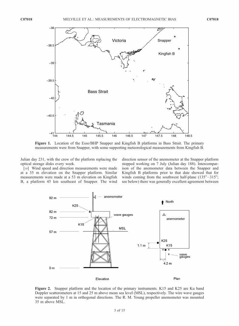
3.4.1. Wave Height[25] Figure 4a compares the time series of the sea surface

elevation h derived from K15, K25 and wire wave gauge C.The data were taken 3 days after the initial calibration underlow wind speeds (U10 � 2.4 m/s). The sea surface fluctua-tions are dominated by swell with Hs = 1.5 m. These valuesare typical of the conditions during the first week of theexperiment. The three instruments are measuring the seasurface elevation at three slightly different horizontal loca-tions (see Figure 2), but show good agreement between theDoppler scatterometers and the wire wave gauge.[26] In general, the two methods give time series that are

comparable except at the crest and troughs of the steepestwaves. At these locations, the wire wave gauge gives largervalues of the wave height than the scatterometers. Thediscrepancies in the wave height measured by the twomethods are due to errors associated with neglectinghigher-order slope terms, terms of O(cs/cl), and the finitesize of the scatterometer footprints.[27] The effects of the differences in the footprint size are

apparent in Figure 4b, which shows typical wave heightfrequency spectra F( f ) derived from K25, K15 and wirewave gauge C. The spectra were computed from �1 hour ofdata and show that while the spectral levels at the energy-containing portion of both scatterometer spectra are nearlyequal, the K25 spectral level falls off at a steeper slopethan that of K15. This shows that of the two scatterometers,K15 is better able to resolve the high-frequency character-istics of the surface wave spectrum.[28] Figure 4b also shows that the spectral level of

wire wave gauge C at frequencies larger than �0.5 Hz isgreater than that for the scatterometer derived spectra, withthe difference increasing at the higher frequencies. Asmentioned earlier, the scatterometer Doppler resolution islimited to waves larger than the size of the footprint whichis in the range of 1–3 m. In contrast, the wire wave gaugemeasurement area is comparable to the wire diameter: a few

millimeters. Hence the wire wave gauge is able to resolvehigher surface wave frequencies much better than eitherscatterometer. An orthogonal regression [Casella, 1990,p. 584] of Hs measured by K15 and K25 gives

Hs K15ð Þ ¼ 1:04Hs K25ð Þ � 0:017 ð11Þ

in meters. That is, the difference in the elevation, andconsequently the spot size, of the two scatterometers leadsto a 4% discrepancy in the Hs estimates.3.4.2. Wave Slope[29] The effect of the difference in the illuminated area,

and consequently the ability of the scatterometers to resolvehigher-frequency waves, is seen more readily when thewave slope spectrum S( f ) is deduced from F( f ), thesurface displacement spectrum. A measure of the rms waveslope s can be computed from F and the linear dispersionrelationship using the relations [Cox and Munk, 1956]

S fið Þ ¼ 2pfið Þ4

g2F fið Þ ð12Þ

s ¼ 1

N

XNi¼1

2pfið Þ4

g2F fið Þ

" #1=2

: ð13Þ

Figure 4c shows plots of the wave slope spectra S( f ) fromK25 and K15 and wire wave gauge C computed usingequation (12) and the wave height spectraF( f ) in Figure 4b.As expected, the differences in the spectral levels of S( f )between the two scatterometers are more pronounced at thehigher frequencies. We can also see that compared to F( f ),the spectral level at the higher frequencies of S( f ) has a moresignificant effect on the value of s. The accurate determina-tion of the full rms wave slope s, is fraught with difficultiesassociated with an appropriate choice of the cutoff frequency,and with the use of the linear dispersion relationship[Felizardo and Melville, 1995]. Recent work [Fedorov etal., 1998] suggests that the cutoff frequency required to givethe full rms wave slope may be as high as O(100) Hz.However, we are only concerned with estimating the con-tribution to the rms slope from waves comparable in scale orlonger than the diameter of the footprint of the scatterometer,sl, say. For these purposes, we can use the cutoff of K15at �1 Hz (see Figure 4b), which leads to larger estimates ofsl from K15 than from K25 as shown in Figure 5a. Linearregression of the data gives

slK15 ¼ 1:12slK25 þ 0:005: ð14Þ

[30] Since the difference between sl computed using thetwo scatterometers can be significant, we will be using slK15as the value of sl in subsequent figures. However, Figure 4suggests that estimates of sl based on K15 may still slightlyunderestimate the rms slope of the longer waves.

3.5. Wave Age

[31] Wave age, the ratio of a characteristic surface wavephase speed to the wind speed, c/U10, is a measure of thestrength of the wind forcing and wave growth. For low

C07018 MELVILLE ET AL.: MEASUREMENTS OF ELECTROMAGNETIC BIAS

6 of 15

C07018

Figure 4. Intercomparisons of (a) surface displacement measurements, (b) wave amplitude spectra, and(c) slope spectra from K15 (dashed lines), K25 (solid lines), and a wire wave gauge (dash-dotted lines) onJulian day 170. Note that the separation of the instruments by horizontal distances of O(1) m account forsome of the differences in Figure 3a but should have no effect on the spectra. The arrows in Figure 3bdenote the cutoff frequencies of 0.9 Hz and 0.7 Hz based on the footprints of K15 and K25, respectively.The small local peaks in the spectra at 0.4–0.5 Hz are most likely due to interference from the leg of theplatform. The ‘‘slope’’ spectrum is based on the wave spectrum and the linear dispersion relationship fordeep water waves and is only an approximation to the true slope spectrum.

C07018 MELVILLE ET AL.: MEASUREMENTS OF ELECTROMAGNETIC BIAS

7 of 15

C07018

values of c/U10, the waves are strongly forced and growthrates, normalized by the wave frequency corresponding to c,are high. For values of wave age around unity the growthrates are very small and may change sign as unity isexceeded [Komen et al., 1994].[32] The wave age is not unique for a given set of

conditions as it depends on the choice of c from a spectrumof surface waves. In our case we choose c to representwaves at the peak of the wind sea spectrum, fp, so cp �c( fp). The wave height spectrum may have peaks repre-senting both wind waves and swell, but the contributionof the swell to the wave slope is generally much lessthan that of the local wind-generated waves. Furthermore,in a preliminary analysis using coherence techniques tostudy the frequencies contributing most to the correlationbetween the surface displacement and backscatteredpower, the source of EM bias, we found the coherenceto be significant only at frequencies greater than the peakof the wind wave spectrum.[33] In the absence of directional wave measurements, we

simply used the presence of multiple peaks in the spectrumto distinguish between wind seas and swell for the purposes

of defining cp. For unimodal spectra, we used the singlepeak to define cp.

3.6. Electromagnetic Bias

[34] The EM bias � is a shift in the mean reflectingsurface measured by the altimeter due to the greater reflec-tivity of the wave troughs than the wave crests. Its value iscomputed from measurements of the scatterometer crosssection s0 and the sea surface elevation h with

� ¼

XN

n¼1s0 tnð Þh tnð ÞXN

n¼1s0 tnð Þ

ð15Þ

at the full temporal resolution of the measurements. If s0and h are completely uncorrelated, then � is equal to zero.

4. Results

[35] Over the 2 month deployment of this experiment,the hourly averaged wind speed U10 ranged from 0.6 to15.4 m/s, the significant wave height Hs from 0.7 to 4.0 m,

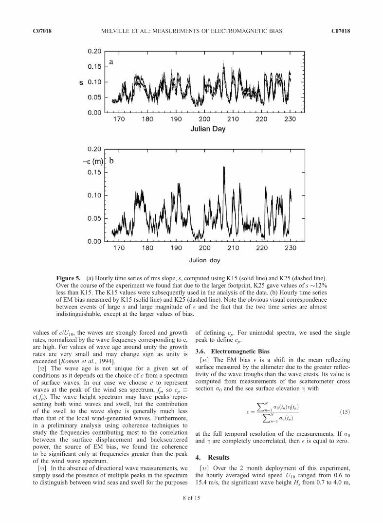
Figure 5. (a) Hourly time series of rms slope, s, computed using K15 (solid line) and K25 (dashed line).Over the course of the experiment we found that due to the larger footprint, K25 gave values of s �12%less than K15. The K15 values were subsequently used in the analysis of the data. (b) Hourly time seriesof EM bias measured by K15 (solid line) and K25 (dashed line). Note the obvious visual correspondencebetween events of large s and large magnitude of � and the fact that the two time series are almostindistinguishable, except at the larger values of bias.

C07018 MELVILLE ET AL.: MEASUREMENTS OF ELECTROMAGNETIC BIAS

8 of 15

C07018

and the rms wave slope s from 0.02 to 0.16. Linear regres-sions between the HH and VV data in the calculation of theEM bias showed that K15HH was 6% smaller than K15VVand K25HH was 3% larger than K25VV. These differencesremain unexplained and for isotropic distributions of thesurface wave field must be considered as measures ofinstrument error in measuring the EM bias. Figure 5b showstime series of the hourly averaged � measured by the HHchannels of the K15 and K25 scatterometers. These data arealmost indistinguishable except at the largest biases. Notethat � is always negative and ranged from�0.005 to�0.16 mduring the course of the experiment.

4.1. EM Bias, Wave Height, and Wind Speed

[36] Figure 6 shows plots of the measured binned nor-malized bias b, for K15 and K25, as a function of U10, withthe residual binned as a function of Hs. Also shown are ~b =b1(U10) + b2(Hs) third-order polynomial fits to b for eachelevation. The data are binned in increments of 1 m/s forU10 and 0.2 m increments for Hs. This traditional way ofdisplaying the data and the polynomial representation interms of the wind speed and significant wave height showsome of the ambiguity that can result as ~b does not go tozero as both U10 and Hs go to zero.[37] It is instructive to display the data in the (U10, Hs)

plane as shown in Figure 7. Here Figure 7a is the measurednormalized bias, bK15, plotted in the plane; Figure 7b is thethird-order polynomial fit to the data; Figure 7c is theresidual, and Figure 7d is the data merged with the poly-nomial fit. The corresponding figure for K25 (not shownhere) is very similar. The polynomial fits for the K15 andK25 data (expressed as a percentage) in the (Hs, U10) planeare

~bK15 ¼� 0:12þ 0:312U10 þ 0:008U210 � 0:001U3

10 þ 1:418Hs

� 0:243H2s � 0:013H3

s ð16Þ

~bK25 ¼ 0:865þ 0:120U10 þ 0:023U 210 � 0:001U3

10 þ 0:716Hs

þ 0:059H2s � 0:059H3

s ; ð17Þ

with standard deviations of 0.61% and 0.54%, respectively.

4.2. EM Bias, Wave Slope, and Wave Age

4.2.1. Polynomial Fits[38] In section 1 we argued that a more rational correla-

tion for the normalized bias, b, would be with the waveslope, sl, and the wave age, or reciprocal wave age, U10/cl.Figure 8 shows the binned normalized bias data for K15 andK25 plotted against these dimensionless variables, alongwith third-order polynomial fits to the data. We use the samenotation as in Figure 6 with ~b = b1(sl) + b2(U10/cl), where b1now represents the binned b data and its polynomial fit as afunction of sl, and b2 represents the residual and itspolynomial fit as a function of U10/cl. Comparison withFigure 6 shows a qualitative and quantitative improvementin the representation of the data using the dimensionlessindependent variables. Most obvious is the reduction in thescatter of the data when plotted against sl (c.f. Figures 6aand 8a). Also, the intercept for b1(s) is essentially zero, andthe range of the residual signal to be correlated with the

wave age, b2(U10/c), is reduced by a factor of 2–3 whencompared with that for b2(Hs).[39] The improved correlations with the dimensionless

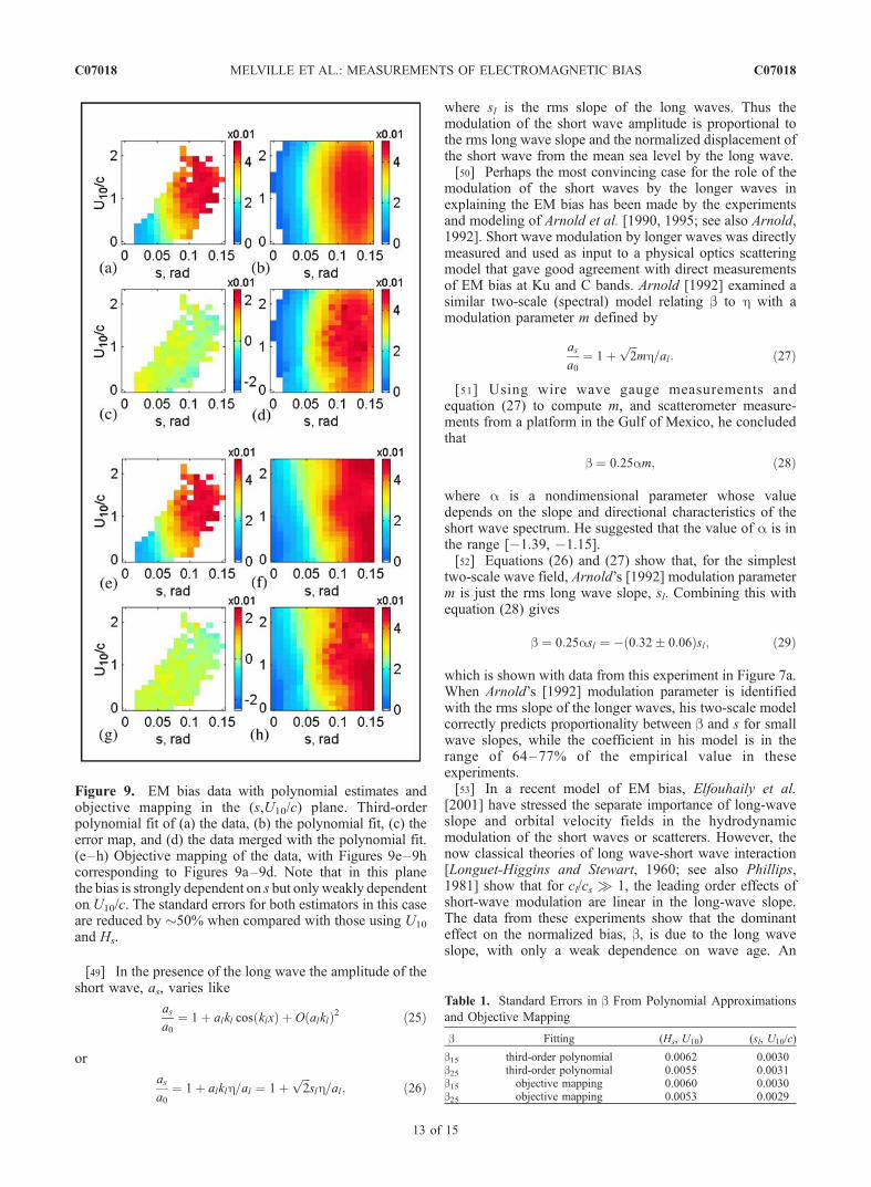
variables become clear when the data for K15 is plotted inthe (s, U10/c) plane as shown in Figure 9a. Also shown isthe third-order polynomial fit to the data (Figure 9b), thedifference between the data and the polynomial fit(Figure 9c), and the data merged with the polynomialfit (Figure 9d). What is immediately clear is that thedependence of b on s is significantly stronger than that onU10/c; that is, the isolines of b are almost vertical. Thecorresponding results for K25 (not shown here) aresimilar. The polynomial fits for K15 and K25 (expressedas a percentage) are

~b15 ¼� 0:458þ 36:3sl þ 294s2l � 2331s3l

þ 0:34U10

clþ 0:28

U10

cl

� �2� 0:17

U10

cl

� �3; ð18Þ

and

~b25 ¼� 0:206þ 42:9sl þ 156s2l � 1829s3l � 0:769U10

clþ 1:264

� U10

cl

� �2� 0:417

U10

cl

� �3; ð19Þ

with standard errors of 0.28% and 0.31%, respectively;�50% less than those for the (Hs, U10) fits. Examination ofthe data in Figure 8 shows that the primary contribution tothe constants in each polynomial fit comes from the residualassociated with the wave age (Figure 8c).4.2.2. Objective Mapping[40] Gaspar and Florens [1998] have recently drawn

attention to the fact that parametric models of the EM biasare not true least squares approximations to the empiricaldata, and that nonparametric methods can yield improvedestimates of the bias. In the context of our measurements,the conclusion is that multivariate polynomial fits of the kindpresented above do not minimize the error between theestimate and the measurements, since they are constrainedby the assumed functional form. One advantage of theparametric models is that they can be represented by a fewparameters, whereas the nonparametric estimates require alook-up table to estimate the bias from the independentvariables. However, this is not a significant disadvantage foraltimetry. In effect, nonparametric, or optimal estimation(objective mapping) techniques, are a way of smoothlyinterpolating the measured data to minimize the mean squareerror between the interpolation and the data.[41] The method used here is a standard implementation

of objective mapping or Gauss-Markov interpolation[Daley, 1991] using the MIT/SaGA software package writ-ten by K. K. Pankratov (1995, see http://puddle.mit.edu/~glenn/kirill/saga.html). On the basis of an analysis of thedata we fitted the empirical correlation of the data to astandard correlation function of the form

C x; yð Þ ¼ ed x; yð Þ þ 1� eð Þ exp � x

Lx

� 2

� y

Ly

� 2" #

; ð20Þ

C07018 MELVILLE ET AL.: MEASUREMENTS OF ELECTROMAGNETIC BIAS

9 of 15

C07018

where, for example, in the (sl, U10/c) space,

x ¼ a s� sið Þ þ 1� a2 �1=2 U10

c� U10

ci

� ð21Þ

y ¼ � 1� a2 �1=2

s� sið Þ þ aU10

c� U10

ci

� ; ð22Þ

where e is the relative error, d is the Dirac delta function, adefines the orientation of the principal axes in the plane, andLx and Ly are decorrelation length scales in the x and ydirections, respectively.[42] Figures 7e–7h show the results of using the

objective mapping to estimate the normalized bias in the(Hs, U10) plane. Overall, we find that the objectivemapping only leads to a marginal improvement in the

Figure 6. Averages (1 hour) and binned normalized EM bias data b = �/Hs, with third-order polynomialfits to U10 and Hs. (a) Scatterplot of hourly averaged data for both K15 and K25. (b) �b and �b1(U10),the polynomial fit to U10 as percentages: K15 (circles and solid line) and K25 (crosses and dashed line).(c) �b2(Hs), the polynomial fit to Hs of the residual where b2 = b � b1. K15 and K25 are as in Figure 6b.Note the nonzero intercepts in both figures.

C07018 MELVILLE ET AL.: MEASUREMENTS OF ELECTROMAGNETIC BIAS

10 of 15

C07018

standard error from 0.0062 to 0.0060, when comparedwith the polynomial fit to the data (Figure 7a).[43] Figures 9e–9h show the corresponding results for

the data in the (sl, (U10/c)) plane. Here there is no improve-ment in the standard error, both being 0.0030.[44] While the use of objective mapping makes no

discernable improvement in the standard error of the biasestimation, the error data tabulated in Table 1, clearly showsthat the use of wave slope and wave age rather than wave

height and wind speed leads to a significant reduction of theerror by 52 ± 2% to 0.003 ± 0.0001. See Table 1.

5. Discussion

[45] While dimensional analysis provides support forthe relationship b = b(alkl, U10/cl,.), it does not give thefunctional form of the relationship nor illuminate thephysical processes. That requires a theory or model. It isclear from Figure 8b that b is proportional to the rms waveslope of the longer waves sl for sl � 1, and essentiallyindependent of the scatterometer elevation in the experi-ment, giving

b � �0:45sl: ð23Þ

[46] A variety of processes related to surface waves andelectromagnetic scattering by the ocean surface can berepresented by an expansion in terms of the surface waveslope and other dimensionless variables including wave ageand the normalized bandwidth of the surface wave spectrum.The principal processes that have been considered inaccounting for the modulation of the scattering that leadsto the EM bias have been short wave (scatterer) modulationand tilt modulation by the longer waves [Arnold et al., 1990;Arnold, 1992; Rodriguez et al., 1992; Elfouhaily et al.,2000], both of which can be represented by expansions interms of the long wave slope. Using a scattering model,Rodriguez et al. [1992] concluded that both effects could beequally important, with the altimeter frequency dependencebeing primarily due to the tilt modulation. Elfouhaily et al.[2000] recently concluded that the short wave effects werenot accurately represented by earlier theories [Srokosz, 1986]but required inclusion of the slope variance ratios thatdepend on the modulation between short and long waves.[47] The data presented here show that the wave age

effects are secondary to those of wave slope, suggesting thatwind forcing (measured by wave age) is a secondary effectalso. In the absence of wind forcing, short waves riding onlonger waves have their wavelengths shortened (length-ened) and amplitudes increased (decreased) at the crest(trough) of the longer waves [Longuet-Higgins and Stewart,1960]. To leading order, the degree of modulation of theshort wave (in amplitude and wave number) is proportionalto the wave slope of the longer wave. Equation (23)suggests that b is proportional to the wave slope, qualita-tively consistent with the degree of short wave modulation.[48] This result can be better understood by representing

the surface wave distribution using a simple two-scalemodel. Consider a simple case where the sea surfaceconsists of two waves, a long wave of length much largerthan the diameter of the illuminated area of the scatterom-eter L, and a short wave of wavelength smaller than L. Theamplitude, wavelength and wave number of the long waveare al, ll and kl, respectively. The reference values of theamplitude, wavelength and wave number of the short waveare a0, l0 and k0. In addition, we assume that al a0.Hence to leading order, the sea surface elevation at a givenlocation along the x axis is

h ¼ al cos klxð Þ: ð24Þ

Figure 7. EM bias data with polynomial and optimalestimates (objective mapping) in the (U10,Hs) plane. Third-order polynomial fit of (a) the data, (b) the polynomial fit,(c) the error map, and (d) the data merged with thepolynomial fit. (e–h) Objective mapping of the data.Figures 7e–7h correspond to Figures 7a–7d. Note thequalitative differences in the estimates of Figures 7b and 7fwhen the different methods are applied. However, thestandard errors for the two methods are essentially the same.See Table 1.

C07018 MELVILLE ET AL.: MEASUREMENTS OF ELECTROMAGNETIC BIAS

11 of 15

C07018

Figure 8. Averages (1 hour) and binned normalized EM bias data b = �/Hs, with third-order polynomialfits to s and U10/c. (a) Scatterplot of hourly averaged data for both K15 and K25. (b) �b and �b1(s), thepolynomial fit to s: K15 (circles and solid line) and K25 (crosses and dashed line). The dashed straightline corresponds to the semiempirical prediction of Arnold [1992]. (c) �b2(U10/c), the polynomial fit toU10/c of the residual where b2 = b � b1. K15 and K25 are as in Figure 8b. Note that the intercept for b1(s)is essentially zero, and the residual in b2 is now within the range ±0.5% over the whole range of theexperiment.

C07018 MELVILLE ET AL.: MEASUREMENTS OF ELECTROMAGNETIC BIAS

12 of 15

C07018

[49] In the presence of the long wave the amplitude of theshort wave, as, varies like

as

a0¼ 1þ alkl cos klxð Þ þ O alklð Þ2 ð25Þ

or

as

a0¼ 1þ alklh=al ¼ 1þ

ffiffiffi2

pslh=al; ð26Þ

where sl is the rms slope of the long waves. Thus themodulation of the short wave amplitude is proportional tothe rms long wave slope and the normalized displacement ofthe short wave from the mean sea level by the long wave.[50] Perhaps the most convincing case for the role of the

modulation of the short waves by the longer waves inexplaining the EM bias has been made by the experimentsand modeling of Arnold et al. [1990, 1995; see also Arnold,1992]. Short wave modulation by longer waves was directlymeasured and used as input to a physical optics scatteringmodel that gave good agreement with direct measurementsof EM bias at Ku and C bands. Arnold [1992] examined asimilar two-scale (spectral) model relating b to h with amodulation parameter m defined by

as

a0¼ 1þ

ffiffiffi2

pmh=al : ð27Þ

[51] Using wire wave gauge measurements andequation (27) to compute m, and scatterometer measure-ments from a platform in the Gulf of Mexico, he concludedthat

b ¼ 0:25am; ð28Þ

where a is a nondimensional parameter whose valuedepends on the slope and directional characteristics of theshort wave spectrum. He suggested that the value of a is inthe range [�1.39, �1.15].[52] Equations (26) and (27) show that, for the simplest

two-scale wave field, Arnold’s [1992] modulation parameterm is just the rms long wave slope, sl. Combining this withequation (28) gives

b ¼ 0:25asl ¼ � 0:32� 0:06ð Þsl; ð29Þ

which is shown with data from this experiment in Figure 7a.When Arnold’s [1992] modulation parameter is identifiedwith the rms slope of the longer waves, his two-scale modelcorrectly predicts proportionality between b and s for smallwave slopes, while the coefficient in his model is in therange of 64–77% of the empirical value in theseexperiments.[53] In a recent model of EM bias, Elfouhaily et al.

[2001] have stressed the separate importance of long-waveslope and orbital velocity fields in the hydrodynamicmodulation of the short waves or scatterers. However, thenow classical theories of long wave-short wave interaction[Longuet-Higgins and Stewart, 1960; see also Phillips,1981] show that for cl/cs 1, the leading order effects ofshort-wave modulation are linear in the long-wave slope.The data from these experiments show that the dominanteffect on the normalized bias, b, is due to the long waveslope, with only a weak dependence on wave age. An

Figure 9. EM bias data with polynomial estimates andobjective mapping in the (s,U10/c) plane. Third-orderpolynomial fit of (a) the data, (b) the polynomial fit, (c) theerror map, and (d) the data merged with the polynomial fit.(e–h) Objective mapping of the data, with Figures 9e–9hcorresponding to Figures 9a–9d. Note that in this planethe bias is strongly dependent on s but only weakly dependenton U10/c. The standard errors for both estimators in this caseare reduced by �50% when compared with those using U10

and Hs.

Table 1. Standard Errors in b From Polynomial Approximations

and Objective Mapping

b Fitting (Hs, U10) (sl, U10/c)

b15 third-order polynomial 0.0062 0.0030b25 third-order polynomial 0.0055 0.0031b15 objective mapping 0.0060 0.0030b25 objective mapping 0.0053 0.0029

C07018 MELVILLE ET AL.: MEASUREMENTS OF ELECTROMAGNETIC BIAS

13 of 15

C07018

anonymous referee suggested that the largest values (of thesmall) residual EM bias occurring at small wave ages (seeFigure 8) could be evidence of contamination by swell;however, comparable values of the residual EM bias occurat the largest wave ages! Furthermore, as mentioned above,a preliminary study of the coherence between the back-scattered power and the surface wave spectrum shows thatthe contribution to the EM bias is predominantly from thelonger waves that contribute most to the slope. This wouldappear to exclude any significant influence of the swell.However, a conclusive study of the influence of swellwould require good directional wave measurements, thatcan separate wind seas and swell by both their directionalproperties and their frequencies.[54] Our use of a constant Charnock parameter in equa-

tion (5), which neglects recent observations of the depen-dence of the parameter on wave age [e.g., Drennan et al.,2003] and other variables may influence the values of U10

used here. The measurement and characterization of thedrag coefficient over the ocean (equivalent to measuring z0)is an important area of current research which goes wellbeyond the limits of this study. However, in this case itsimportance is mitigated by the secondary role of the residualEM bias which is not accounted for by the wave slope andis correlated here with the wave age which depends on U10.Nevertheless, it points to the need for further direct mea-surements of EM bias with state-of-the-art atmosphericboundary layer measurements in which u* is directlymeasured and the applicability of Monin-Obukhov scalingof the atmospheric boundary layer is tested.[55] Together the use of wave slope and wave age rather

than wind speed and wave height leads to a reduction by�50% in the error of the EM bias estimates. These improve-ments are independent of whether we use polynomial fits orobjective mapping of the data. We believe that thesereductions in the errors are sufficient to justify an exami-nation of how information on wave slope and wave age canbe included in operational algorithms for EM bias. Glazmanand Srokosz [1991] have suggested that ‘‘pseudo’’ waveparameters (especially wave age) might be inferred from theclassical fetch relationships for wind waves, but there aregood reasons why this approach would not work in altim-etry. One of the principal uses of radar altimetry is in usingthe measured sea surface slope to infer the geostrophiccurrents, the classical examples being across westernboundary currents over which the sea surface height mayvary by O(1) m. However, wave-current interaction cansignificantly modify the slope of the surface waves, espe-cially in current gradients, and, according to the measure-ments presented here, modify the EM bias. Thus the bias iscorrelated with the desired measurement in a way thatcannot be resolved unless the slope is directly measured,or inferred from a model that accounts for these effects. Webelieve that efforts to globally measure and model thesurface wave field in support of radar altimetry will leadto significantly improved algorithms for EM bias.[56] The beginnings of this approach are explored in a

very recent paper by Kumar et al. [2003]. They consideredthe use of operational wave model (WAM) data and buoymeasurements of the wind and wave field to implement aversion of the empirical wave-slope/wave-age algorithmbased on the data from this work, finding good agreement

with the theoretical EM bias model of Srokosz [1986] over arange of parameters. However, more work is needed toextend the range of wave slopes. They found a significantcorrelation between high-frequency sea surface height fluc-tuations and operational EM bias corrections based onsatellite data and variance minimization techniques [Gasparet al., 1994]. This implies that improved operational EMbias algorithms cannot be based on altimeter data alone, andmay require input from wind wave and coupled ocean-atmosphere models and perhaps other satellite sensors.[57] Following this semiempirical investigation of the

role of the sea surface slope in the representation of theEM bias, which has shown the correspondence betweenthe wave slope and the modulation parameter in the two-scale physical optics model, K. F. Warnick et al. (Theoret-ical model of electromagnetic bias based on RMS waveslope, submitted to Journal of Geophysical Research, 2002)have developed a slightly improved version of the two-scalemodel proposed by Arnold et al. [1991] and Arnold [1992],which gives very good agreement with the Ku bandmeasurements of Arnold et al. [1995] from the Gulf ofMexico. The agreement to within 10% of the best linear fitto the Gulf of Mexico data contrasts with the 23–36%difference with this data from Bass Strait. These differencesbetween the data sets, which were obtained with the sameequipment and techniques, remain unresolved.[58] It is still the case that a complete data set over a wide

range of environmental conditions, including direct mea-surements of EM bias, the directional spectrum of thesurface wave field, sea surface height and surface currentsand winds, which would permit a thorough investigation ofEM bias for operational altimetry, does not exist. In view ofthe critical role of altimetry in global oceanography, air-seainteraction and climate sciences, it is imperative that errorsin estimating EM bias be improved to avoid misinterpretingunresolved bias errors as seasonal, interannual or secularsignals in sea surface height and currents.

[59] Acknowledgments. This experiment would not have been pos-sible without the generosity of Esso/BHP in permitting us to use theplatform and without the efforts of the superintendent and crew of theSnapper Platform in monitoring the data acquisition for a 3 month period.We thank Ian Jones of Sydney University for facilitating these efforts andLawson and Treloar (Australia) for supplying meteorological data from theKingfish B platform. We thank Ron Horn for software development andinstallation, Eric Terrill for logistical support of the experiment, and AnatolRozenberg for preparation and calibration of the scatterometers. We thanktwo anonymous referees of the original paper for their helpful commentsand questions. This work was supported by a grant to W.K.M. from NASAand by a subcontract from Brigham Young University.

ReferencesArnold, D. V. (1992), Electromagnetic bias in radar altimetry at microwavefrequencies, Ph.D. thesis, Mass. Inst. of Technol., Cambridge.

Arnold, D. V., W. K. Melville, and J. A. Kong (1990), Theoretical predic-tion of EM bias, in Oceans 90 Proceedings: Engineering in the OceanEnvironment, pp. 253–256, IEEE Press, Piscataway, N. J.

Arnold, D. V., J. A. Kong, and W. K. Melville (1991), Physical opticsprediction of EM bias, in Proceedings, Progress in ElectromagneticResearch, 169 pp., IEEE Press, Piscataway, N. J.

Arnold, D. V., W. K. Melville, R. H. Stewart, J. A. Kong, W. C. Keller, andE. Lamarre (1995), Measurements of electromagnetic bias at Ku andC bands, J. Geophys. Res., 100, 969–980.

Casella, G. (1990), Statistical Inference, 650 pp., Brooks/Cole, PacificGrove, Calif.

Chelton, D. B. (1994), The sea state bias in altimeter estimates of sea levelfrom collinear analysis of TOPEX data, J. Geophys. Res., 99, 24,995–25,008.

C07018 MELVILLE ET AL.: MEASUREMENTS OF ELECTROMAGNETIC BIAS

14 of 15

C07018

Cox, C. S., and W. H. Munk (1956), Slopes of the sea surface deduced fromphotographs of sun glitter, Bull. Scripps Inst., 6, 401–488.

Daley, R. (1991), Atmospheric Data Analysis, 457 pp., Cambridge Univ.Press, New York.

Doviak, R. J., and D. S. Zrnic (1984), Doppler Radar and WeatherObservations, 458 pp., Academic, San Diego, Calif.

Drennan, W. M., H. C. Graber, D. Hauser, and C. Quentin (2003), On thewave age dependence of wind stress over pure wind seas, J. Geophys.Res., 108(C3), 8062, doi:10.1029/2000JC000715.

Elfouhaily, T., D. R. Thompson, B. Chapron, and D. Vandemark (2000),Improved electromagnetic bias theory, J. Geophys. Res., 105, 1299–1310.

Elfouhaily, T., D. R. Thompson, B. Chapron, and D. Vandemark (2001),Improved electromagnetic bias theory: Inclusion of hydrodynamicmodulations, J. Geophys. Res., 106, 4655–4664.

Fedorov, A. V., W. K. Melville, and A. Rozenberg (1998), An experimentaland numerical study of parasitic capillary waves, Phys. Fluids, 10, 1315–1323.

Felizardo, F. C., and W. K. Melville (1995), Correlations between ambientnoise and the ocean surface wave field, J. Phys. Oceanogr., 25, 513–532.

Gaspar, P., and J.-P. Florens (1998), Estimation of the sea state bias in radaraltimeter measurements of sea level: Results from a new nonparametricmethod, J. Geophys. Res., 103, 15,803–15,814.

Gaspar, P., F. Ogor, P.-Y. Le Traon, and O.-Z. Zanife (1994), Estimating thesea state bias of the TOPEX and Poseidon altimeters from crossoverdifferences, J. Geophys. Res., 99, 24,981–24,994.

Glazman, R., and M. Srokosz (1991), Equilibrium wave spectrum and seastate bias in altimetry, J. Phys. Oceanogr., 21, 1609–1621.

Gommenginger, C. P., M. A. Srokosz, J. Wolf, and P. A. E. M. Janssen(2003), An investigation of altimeter sea state bias theories, J. Geophys.Res., 108(C1), 3011, doi:10.1029/2001JC001174.

Hevizi, L. G., E. J. Walsh, R. E. McIntosh, D. Vandemark, D. E. Hines,R. N. Swift, and J. F. Scott (1993), Electromagnetic bias in sea surfacerange measurements at frequencies of the TOPEX/Poseidon satellite,IEEE Trans. Geosci. Remote Sens., 31, 367–388.

Jessup, A. T. (1990), Detection and characterization of deep-water wavebreaking using moderate incidence angle microwave backscatter from thesea surface, Ph.D. thesis, Mass. Inst. of Technol.-Woods Hole Oceanogr.Inst. Joint Prog., Cambridge, Mass.

Jessup, A. T., W. K. Melville, and W. C. Keller (1991), Breaking wavesaffecting microwave backscatter: 1. Detection and verification, J. Geo-phys. Res., 96, 20,547–20,559.

Komen, G. J., L. Cavaleri, M. Donelan, K. Hasselmann, S. Hasselman, andP. A. E. M. Janssen (1994), Dynamics and Modelling of Ocean Waves,532 pp., Cambridge Univ. Press, New York.

Kumar, R., D. Stammer, W. K. Melville, and P. Janssen (2003), Electro-magnetic bias estimates based on TOPEX, buoy, and wave model data,J. Geophys. Res., 108(C11), 3351, doi:10.1029/2002JC001525.

Large, W. G., and S. Pond (1981), Open ocean momentum flux measure-ments in moderate to strong winds, J. Phys. Oceanogr., 11, 324–336.

Longuet-Higgins, M. S., and R. W. Stewart (1960), Changes in the form ofshort gravity waves on long waves and tidal currents, J. Fluid Mech., 8,565–583.

Melville, W. K., R. H. Stewart, W. C. Keller, J. A. Kong, D. V. Arnold, A. T.Jessup, M. R. Loewen, and A. M. Slinn (1991), Measurements of elec-tromagnetic bias in radar altimetry, J. Geophys. Res., 96, 4915–4924.

Melville, W. K., F. C. Felizardo, and P. Matusov (1999), Measurementsof sea-state bias, poster presented at the Air-Sea Interface Symposium,Sydney, 11–15 Jan.

Millet, F. W., D. V. Arnold, K. F. Warnick, and J. Smith (2003a), Electro-magnetic bias estimation using in situ and satellite data: 1. RMS waveslope, J. Geophys. Res., 108(C2), 3040, doi:10.1029/2001JC001095.

Millet, F. W., D. V. Arnold, P. Gaspar, K. F. Warnick, and J. Smith (2003b),Electromagnetic bias estimation using in situ and satellite data: 2. Anonparametric approach, J. Geophys. Res., 108(C2), 3041, doi:10.1029/2001JC001144.

Phillips, O. M. (1981), The dispersion of short wavelets in the presence of adominant long wave, J. Fluid Mech., 107, 465–485.

Rodriguez, E., Y. Kim, and J. M. Martin (1992), The effect of small-wavemodulation on the electromagnetic bias, J. Geophys. Res., 97, 2379–2389.

Smith, S. D. (1988), Coefficients for sea surface wind stress, heat flux, andwind profiles as a function of wind speed and temperature, J. Geophys.Res., 93, 15,467–15,472.

Srokosz, M. (1986), On the joint distribution of surface elevation andslopes for a nonlinear random sea, with an application to radar altimetry,J. Geophys. Res., 91, 995–1006.

Walsh, E. J., et al. (1991), Frequency dependence of electromagnetic bias inradar altimeter sea surface range measurements, J. Geophys. Res., 96,20,571–20,583.

Wu, J. (1980), Wind stress coefficients over the sea surface near neutralconditions—A revisit, J. Phys. Oceanogr., 10, 727–740.

Yaplee, B., A. Shapiro, D. Hammond, B. Au, and E. Uliana (1971), Nano-second radar observations of the ocean surface from a stable platform,IEEE Trans. Geosci. Electron., 9, 170–174.

�����������������������F. C. Felizardo, Union Cement Corporation, 39 Plaza Drive, Rockwell

Center, Makati City, Philippines. (fcf.ucc@phinma.com.ph)W. K. Melville and P. Matusov, Scripps Institution of Oceanography,

University of California, San Diego, La Jolla, California, 92093-0213,USA. (kmelville@ucsd.edu; pmatusov@ucsd.edu)

C07018 MELVILLE ET AL.: MEASUREMENTS OF ELECTROMAGNETIC BIAS

15 of 15

C07018