6 Waveguide Arrays for Optical Pulse-Shaping, Mode-Locking and Beam Combining J. Nathan Kutz Department of Applied Mathematics, University of Washington USA 1. Introduction Nonlinear mode-coupling (NLMC) is a well-established phenomenon which has been both experimentally verified (1; 2; 3; 4; 5) and theoretically characterized (6; 7; 8). NLMC has been an area of active research in all-optical switching and signal processing applications using wave-guide arrays (2; 3; 4; 5), dual-core fibers (1; 6; 7), and fiber arrays (9; 10). Recently, the temporal pulse shaping associated with NLMC has been theoretically proposed for the passive intensity-discrimination element in a mode-locked fiber laser (11; 12; 13; 14; 15; 16). The models derived to characterize the mode-locking consist of two governing equations: one for the fiber cavity and a second for the NLMC element (11; 12; 13; 16) (See Fig. 1). Although the two discrete components provide accurate physical models for the laser cavity, analytic methods for characterizing the underlying laser stability and dynamics is often rendered intractable. Thus, it is often helpful to construct an averaged approximation to the discrete components model in order to approximate and better understand the mode- locking behavior. Indeed, this is the essence of Haus’ master mode-locking theory (17). Here, we develop an averaged approximation to the discrete laser cavity system based upon NLMC and characterize the resulting laser cavity dynamics. The resulting averaged equations are the equivalent of a master mode-locking theory for a laser cavity based upon nonlinear mode-coupling. From an applications point of view, high-power pulsed lasers are an increasingly important technological innovation as their conjectured and envisioned applications have grown significantly over the past decade. Indeed, this promising photonic technology has a wide number of applications ranging from military devices and precision medical surgery to optical interconnection networks (17; 18; 19; 20). Such technologies have placed a premium on the engineering and optimization of mode-locked laser cavities that produce stable and robust high-power pulses. Thus the technological demand for novel techniques for producing and stabilizing high-power pulses has pushed mode-locked lasers to the forefront of commercially viable, nonlinear photonic devices. The performance of the waveguide array mode-locking model developed is optimized so as to produce high-power pulses in both the anomalous and normal dispersion regimes. The stability of the mode- locked solutions are completely characterized as a function of the cavity energy and the waveguide array parameters. In principle, operation of a mode-locked laser (17; 18) is achieved using an intensity discrimination element in a laser cavity with bandwidth limited gain (17). The intensity www.intechopen.com
Transcript
6
Waveguide Arrays for Optical Pulse-Shaping, Mode-Locking and Beam Combining
J. Nathan Kutz Department of Applied Mathematics, University of Washington
USA
1. Introduction
Nonlinear mode-coupling (NLMC) is a well-established phenomenon which has been both experimentally verified (1; 2; 3; 4; 5) and theoretically characterized (6; 7; 8). NLMC has been an area of active research in all-optical switching and signal processing applications using wave-guide arrays (2; 3; 4; 5), dual-core fibers (1; 6; 7), and fiber arrays (9; 10). Recently, the temporal pulse shaping associated with NLMC has been theoretically proposed for the passive intensity-discrimination element in a mode-locked fiber laser (11; 12; 13; 14; 15; 16). The models derived to characterize the mode-locking consist of two governing equations: one for the fiber cavity and a second for the NLMC element (11; 12; 13; 16) (See Fig. 1). Although the two discrete components provide accurate physical models for the laser cavity, analytic methods for characterizing the underlying laser stability and dynamics is often rendered intractable. Thus, it is often helpful to construct an averaged approximation to the discrete components model in order to approximate and better understand the mode-locking behavior. Indeed, this is the essence of Haus’ master mode-locking theory (17). Here, we develop an averaged approximation to the discrete laser cavity system based upon NLMC and characterize the resulting laser cavity dynamics. The resulting averaged equations are the equivalent of a master mode-locking theory for a laser cavity based upon nonlinear mode-coupling. From an applications point of view, high-power pulsed lasers are an increasingly important technological innovation as their conjectured and envisioned applications have grown significantly over the past decade. Indeed, this promising photonic technology has a wide number of applications ranging from military devices and precision medical surgery to optical interconnection networks (17; 18; 19; 20). Such technologies have placed a premium on the engineering and optimization of mode-locked laser cavities that produce stable and robust high-power pulses. Thus the technological demand for novel techniques for producing and stabilizing high-power pulses has pushed mode-locked lasers to the forefront of commercially viable, nonlinear photonic devices. The performance of the waveguide array mode-locking model developed is optimized so as to produce high-power pulses in both the anomalous and normal dispersion regimes. The stability of the mode-locked solutions are completely characterized as a function of the cavity energy and the waveguide array parameters. In principle, operation of a mode-locked laser (17; 18) is achieved using an intensity discrimination element in a laser cavity with bandwidth limited gain (17). The intensity
www.intechopen.com
Numerical Simulations - Applications, Examples and Theory
122
(b)
arraywaveguide
Erbium fiber
outputcoupler
mirror
outputoupler
Erbium fiber
waveguide array
(a)
Fig. 1. Two possible laser cavity configurations which include nonlinear mode-coupling from the waveguide array as the mode-locking element. The fiber coupling in and out of the waveguide array occurs at the central waveguide as illustrated. Any electromagnetic field which is propagated into the neighboring waveguides is ejected (attenuated) from the laser cavity. In addition to the basic setup, polarization controllers, isolators, and other stabilization mechanisms may be useful or required for successful operation.
discrimination preferentially attenuates weaker intensity portions of individual pulses or electromagnetic energy. This attenuation is compensated by the saturable gain medium (e.g. Erbium-doped fiber). Pulse narrowing occurs since the peak of a pulse, for instance, experiences a higher net gain per round trip than its lower intensity wings. This pulse compression is limited by the bandwidth of the gain medium (typically ≈ 20 – 40 nm (17; 18)). It is well understood that some form of cavity saturable absorption or intensity discrimination is fundamental to producing stable mode-locked pulses in a passive laser cavity (17; 19; 23). Such intensity discrimination can be produced by a number of methods ranging from placing a linear polarizer in a fiber ring laser (24; 25; 26; 27), using a coupler in a figure-eight laser to produce nonlinear interferometry (28; 29; 30; 31), placing a semiconductor saturable absorber in a linearcavity configuration (32; 33; 34), or using a combination of spectral filtering with polarization filters in a dispersion controlled cavity (35; 36; 37; 38). Alternatively, active mode-locking can be used to produce mode-locked pulses by directly modulating the output electromagnetic field or using an acousto-optic modulator (40; 41). In all these cases, an effective intensity discrimination is generated to stabilize and control the mode-locked pulses. A relatively new method for generating intensity discrimination in a laser cavity is due to the nonlinear mode-coupling generated in a waveguide array (11; 12; 13; 21; 22). Although nonlinear mode-coupling has been proposed previously as a theoretical method for producing stable mode-locking (14; 16; 15), the waveguide array is the only nonlinear mode-coupling device that has been experimentally verified to produce the requisite pulse shaping required for mode-locking (42). This intensity discrimination, which is often only a small perturbation to the laser cavity dynamics, can be achieved with NLMC due to the well-known discrete self-focusing properties of the NLMC element. Indeed, the NLMC dynamics in wave-guide arrays is well-documented experimentally and provides the motivation for the current work. An overview of the techniques and methods which are capable of producing intensity discrimination and
www.intechopen.com
Waveguide Arrays for Optical Pulse-Shaping, Mode-Locking and Beam Combining
123
mode-locking are reviewed in Refs. (17; 23). Although theoretical models have been developed towards understanding the mode-locking dynamics and stability of waveguide array based lasers (11; 12; 13; 21; 22), a characterization of its optimal performance and ability to generate high peak-power and high-energy pulses has not previously been performed. Figure 1 illustrates two possible mode-locking configurations in which the waveguide array provides the critical effect of intensity discrimination (saturable absorption). In Fig. 1(a) a linear cavity configuration is considered whereas in Fig. 1(b) a ring cavity geometry is considered. In either case, the waveguide array provides an intensity dependent pulse shaping by coupling out low intensity wings to the neighboring waveguides. This low intensity field is then ejected from the laser cavity. In contrast, high intensity portions of the pulse are retained in the central waveguide due to self-focusing. Thus high intensities are only minimally attenuated. This intensity selection mechanism generates the necessary pulse shaping for producing stable mode-locked pulse trains.
2. Governing equations
In addition to the cavity (fiber) propagation equations, theoretical models are required to describe the NLMC element. Although nonlinear mode-coupling can be achieved in at least three ways (13) (wave-guide arrays, dual-core fibers, and fiber arrays), we will consider only wave-guide arrays since they illustrate all the basic properties of NLMC based mode-locking. The NLMC models are fundamentally the same, the only difference being in the number of modes coupled together. It should be noted that the NLMC theory presented here is an idealization of the dynamics of the full Maxwell’s equations. For very short temporal pulses (i.e. tens of femtoseconds or less), modifications and corrections to the theory may be necessary.
2.1 Fiber propagation The theoretical model for the dynamic evolution of electromagnetic energy in the laser cavity is composed of two components: the optical fiber and the NLMC element. The pulse propagation in a laser cavity is governed by the interaction of chromatic dispersion, self-phase modulation, linear attenuation, and bandwidth limited gain. The propagation is given by (17)
2 2
22 2
1| | ( ) 1 0 ,
2
Q Qi Q Q i Q ig Z Q
Z T Tγ τ⎛ ⎞∂ ∂ ∂+ + + − + =⎜ ⎟⎜ ⎟∂ ∂ ∂⎝ ⎠ (1)
where
02
0
2( ) ,
1 /
gg Z
Q e= +‖ ‖
(2)
Q represents the electric field envelope normalized by the peak field power 20| ,|Q and
2 2| | .Q Q dT∞−∞= ∫‖ ‖ Here the variable T represents the physical time in the rest frame of the
pulse normalized by T0/1.76 where T0=200 fs is the typical full-width at half-maximum of the pulse. The variable Z is scaled on the dispersion length 2 2
0 0 0(2 ) /( )( /1.76)Z c D Tπ λ= corresponding to an average cavity dispersion 12 ps /km-nm.D≈ This gives the one-soliton
www.intechopen.com
Numerical Simulations - Applications, Examples and Theory
124
peak field power 20 0 eff 2 0| | /(4 ).Q A n Zλ π= Further, n2 = 2.6×10⁻¹⁶ cm2/W is the nonlinear
coefficient in the fiber, Aeff = 60 μm2 is the effective cross-sectional area, λ0 = 1.55 μm is the free-space wavelength, c is the speed of light, and γ = ΓZ0 (Γ = 0.2 dB/km) is the fiber loss. The bandwidth limited gain in the fiber is incorporated through the dimensionless parameters g and τ = (1/Ω2)(1.76/T0)2. For a gain bandwidth which can vary from
2020 40 , (2 / )nm cλ π λ λΔ = − Ω = Δ so that τ ≈ 0.08–0.32. The parameter τ controls the spectral
gain bandwidth of the mode-locking process, limiting the pulse width. It should be noted that a solid-state configuration can also be used to construct the laser cavity. As with optical fibers, the solid state components of the laser can be engineered to control the various physical effects associated with (1). Given the robustness of the mode-locking observed, the theoretical and computational predictions considered here are expected to hold for the solid-state setup. Indeed, the NLMC acts as an ideal saturable absorber and even large perturbations in the cavity parameters (e.g. dispersion-management, attenuation, polarization rotation, higher-order dispersion, etc.) do not destabilize the mode-locking.
2.2 Nonlinear mode-coupling equations The leading-order equations governing the nearest-neighbor coupling of electromagnetic energy in the waveguide array is given by (2; 3; 4; 5; 8)
21 1( ) | | 0 ,n
n n n n
dAi C A A A A
dβξ − ++ + + = (3)
where An represents the normalized amplitude in the nth waveguide (n = –N, … ,–1, 0, 1, … , N and there are 2N + 1 waveguides). The peak field power is again normalized by 2
0| |Q as in Eq. (1). Here, the variable ξ is scaled by the typical waveguide array length (4) of
0Z∗ =6 mm. This gives C = c 0Z∗ and β = (γ * 0Z∗ /γ Z0). To make connection with a physically realizable waveguide array (5), we take the linear coupling coefficient to be c = 0.82 mm–1
and the nonlinear self-phase modulation parameter to be γ * = 3.6 m–1W–1. Note that for the fiber parameters considered, the nonlinear fiber parameter is γ = 2πn2/(λ0Aeff)=0.0017 m–1W–1. These physical values give C = 4.92 and β = 15.1. The periodic waveguide spacing is fixed so that the nearest-neighbor linear coupling dominates the interaction between waveguides. Over the distances of propagation considered here (e.g. 0Z∗ = 6 mm), dispersion and linear attenuation can be ignored in the wave-guide array. The values of the linear and nonlinear coupling parameters are based upon recent experiment (4). For alternative NLMC devices such as dual-core fibers or fiber arrays, these parameters can be changed substantially. Further, in the dual-core fiber case, only two wave-guides are coupled together so that the n=0 and n=1 are the only two modes present in the dynamic interaction. For fiber arrays, the hexagonal structure of the wave-guides couples an individual wave-guide to six of its nearest neighbors. Regardless of these model modifications, the basic NLMC dynamics remains qualitatively the same.
2.3 Mode-locking via NLMC The self-focusing property of the wave-guide array is what allows the mode-locking to occur. The proto-typical example of the NLMC self-focusing as a function of input intensity is illustrated in Fig. 2a which is simulated with 41 (N = 20) waveguides (5) for two different
www.intechopen.com
Waveguide Arrays for Optical Pulse-Shaping, Mode-Locking and Beam Combining
125
launch powers. For this simulation, light was launched in the center waveguide with initial amplitude A0(0) = 1 (top) and A0(0) = 3 (bottom). Lower intensities are clearly diffracted via nearest-neighbor coupling whereas the higher intensities remain spatially localized due to self-focusing. The spatial self-focusing can be intuitively understood as a consequence of (3) being a second-order accurate, finite-difference discretization of the focusing nonlinear Schrödinger equation (8). This fundamental behavior has been extensively verified experimentally (2; 3; 4; 5). When placed within an optical fiber cavity, the pulse shaping associated with Fig. 2a leads to robust and stable mode-locking behavior (11; 12; 13). The computational model considered in this subsection evolves (1) while periodically applying (3) every round trip of the laser cavity (See Fig. 1). The simulations assume a cavity length of 5 m and a gain bandwidth of 25 nm (τ ≈ 0.1). The loss parameter is taken to be γ = 0.1 which accounts for losses due to the output coupler and fiber attenuation. To account for the significant butt-coupling losses between the waveguide array and the optical fiber, an additional loss is taken at the beginning and end of the waveguide array. Figure 2b demonstrates the stable mode-locked pulse formation over 40 round trips of the laser cavity starting from noisy initial conditions with a coupling loss in and out of the waveguide array of 20% and with a constant gain g0 = 0.7. Due to the excellent intensity discrimination properties of the waveguide array, the mode-locked laser converges extremely rapidly to the steady-state mode-locked solution. It is this generation of a stabilized mode-locked soliton pulse which the averaged model needs to reproduce. Note that the gain level g0 has been chosen so that only a single pulse per round trip is supported. Further, in Fig. 2b the initial condition is chosen for convenience only.
(a) (b)
Fig. 2. (a) The classic representation of spatial diffraction and confinement of electromagnetic energy in a waveguide array considered by Peschel et al. (5). In the top figure, the intensity is not strong enough to produce self-focusing and confinement in the center waveguide, whereas the bottom figure shows the self-focusing due to the NLMC. Note that light was launched in the center waveguide with initial amplitude a0(0) = 1 (top) and a0(0) = 3 (bottom). (b) Stable mode-locking using a waveguide array with g0 = 0.7. The mode-locking is robust to the specific gain level, cavity parameter changes, and cavity perturbations. Here is is assumed that a 20% coupling loss occurs at the input and output of the waveguide array due to butt-coupling (See Fig. 1b).
www.intechopen.com
Numerical Simulations - Applications, Examples and Theory
126
3. Pulse-shaping and X-waves in normal dispersion cavities
To illustrate the pulse shaping properties and the spontaneous formation of an X-wave structure in the normal GVD regime (43), we integrate numerically the proposed infinite-dimensional map by alternating Eqs. (1) and (2) for a length Lf and Eqs. (3) for a length La. Thus Q of Eq. (1) becomes A0 in Eq. (3) when entering or leaving the waveguide array. Importantly, upon exiting the WGA, the system is strongly perturbed since the energy from all the neighboring channels (Ai where i = ±1, 2, 3, ...) are expelled from the laser cavity. Nevertheless, we observe the formation of a stable mode-locked pulse which shows the field A0 at the output. The white-noise is quickly reshaped (over 10 round trips) into the mode-locking pulse of interest. Thus the mode-locking pulse acts as a global attractor to the laser cavity system. The simulation further implies that the mode-locking behavior is stable in the sense of Floquet (50) since it is a periodic solution in the cavity. The spectral shape clearly indicates that the mode-locking pulse is highly chirped, in analogy to what is found for 1D (no spatial dynamics) solutions of the master mode-locking equations in the normal GVD regime (17). The overall electromagnetic field actually experiences a strong spatio-temporal reshaping per cavity round trip that involves stable coupling of a significant portion of the incoming WGA power to neighboring waveguides with nontrivial timing. The input and output time-domain intensities in all the waveguides, once nonlinear mode-locking has been achieved are displayed in Fig. 3. As shown, the interplay of accumulated GVD, discrete diffraction, and nonlinearity drives the field into a self-organized nonlinear X-waves, whose main signature is a central peak accompanied by pulse splitting occurring in the external channels. To show more clearly the X-shape of the mode-locking wave-packet generated at the ouput (B) of the waveguide array, Fig. 4 depicts a topographical plot of the time-domain (top) of all the waveguides. The distinctive X-wave structure is clearly evident. To lend further evidence to the existence of the X-wave structure, we plot the 2D Fourier transform of the time-domain. The right panel of Fig. 4 demonstrates that the spectrum is also X-shaped, as expected for X-waves (45; 46).
output
-20-10
010
20
-20
0
200
0.5
1
Time T
input
Waveguides
|Q
|2
-20-10
010
20
-20
0
200
0.5
1
Time TWaveguides
|Q
|2
Fig. 3. Input (A) and output (B) temporal power distribution in the WGA. At the input, energy is only launched in the center waveguide (A0), while at the output the energy has spontaneously formed into the X-wave configuration involving about eleven guides. Only energy in the A0 mode is preserved upon re-entry into the fiber section of the cavity.
www.intechopen.com
Waveguide Arrays for Optical Pulse-Shaping, Mode-Locking and Beam Combining
127
Fig. 4. Time-domain profiles and its two-dimensional Fourier transform at the output (B) in the WGA after steady-state mode-locking has been achieved. The X-wave structure is clearly seen in the topographical plot (top) of the output time-domain profiles of Fig. 3. Further, the expected wavenumber versus frequency dependence in the X-wave is shown in the Fourier domain (bottom).
-20-1001020
030
60
0
0.25
0.5
Time TRound Trips
|A
1|
-20-1001020
030
60
0
0.25
0.5
Time TRound Trips
|A
3|
-20-1001020
030
60
0
0.25
0.5
Time TRound Trips
|A
2|
-15 -10 -5 0 5 10 150
0.5
1
1.5
2
Waveguide
Po
wer
Fig. 5. Evolution to the steady-state output (B) in the neighboring waveguides A1, A2, and A3. The bottom right graph is a bar graph of the steady-state distribution of energy
2( | | )jA dT∞−∞∫ in the waveguides. The symmetry about the center waveguide results from
the initial condition being applied only in this waveguide. Note the significant re-distribution of energy in the waveguides.
To further characterize the mode-locking X-wave dynamics, Fig. 5 illustrates the mode-locking to the global attractor in the neighboring waveguides A1, A2 and A3. Once again, generic white-noise initial data quickly self-organize into the steady-state mode-locking pattern. Note the characteristic pulse splitting (dip in the power) in the neighboring waveguides. This shows, in part, the generated X-wave structure. The final panel in Fig. 5 gives the energy 2( | | )jA dT
∞−∞∫ in each of the waveguides and shows that a significant
portion (more than 50%) of the electromagnetic energy has coupled to the neighboring waveguides. This is in sharp contrast to mode-locking with anomalous GVD for which less
www.intechopen.com
Numerical Simulations - Applications, Examples and Theory
128
than 6% is lost to the neighboring waveguides (13) and no stable X-waves are formed. The significant loss of energy in the cavity to the neighboring waveguides is compensated by the gain section and shows that the laser cavity is a strongly damped-driven system.
4. Averaged evolution models
The principle concept behind the averaging method presented here is to derive a single, self-consistent, and asymptotically correct representation of the dynamics in the laser cavity. In order to do so, we require an equation of evolution for each individual wave-guide which accounts for both the fiber propagation and wave-guide array coupling. Thus the term averaged equations refers to the governing set of equations which account for the average effect of dispersion, self-phase modulation, mode-coupling, attenuation, and bandwidth-limited gain in the wave-guide array based laser cavity configuration of Fig. 1. The following important guidelines must be met: • Individual wave-guides are subject to chromatic dispersion and self-phase modulation. • Coupling between neighboring wave-guides is a linear process with coupling
coefficient C. • The central wave-guide A0 is subject to bandwidth-limited gain given in (1) and (2)
since this wave-guide is coupled back into the fiber laser cavity. No other wave-guides experience gain due to amplification.
• The wave-guides neighboring the central wave-guide experience large attenuation due to the fact that they do not couple back into the laser cavity.
These simple guidelines, along with the governing equations (1), (2) and (3), allow for an asymptotically correct averaged description of the laser cavity dynamics. Figure 6 shows a schematic of the averaging process which includes five wave-guides. Specifically, each wave-guide Ai is subject to two distinct physical propagation regions: the optical fiber region and the wave-guide array region. The period L of the laser cavity depicted theoretically in Fig. 6 is established with mirrors as demonstrated in Fig. 1. In the averaging process, only the center wave-guide A0 experiences bandwidth-limited gain as given by (1) with (2) since this wave-guide contains the only optical fiber which has an Erbium doped section of fiber and physically butt-couples in and out of the wave-guide array (see Fig. 1). The optical fibers A±1 and A±2 representing the connection between wave-guide arrays are fictitious and only for averaging purposes. Indeed, as demonstrated in Fig. 1 the energy in the neighboring wave-guide arrays are allowed to escape the cavity into free-space. Put another way, one can think of the optical fiber propagation links in A±1 and A±2 in Fig. 6 as being governed by (1) with large attenuation but no gain, no dispersion, and no self-phase modulation. It should be noted that the attenuation in the neighboring wave-guides A±1 may not be too large since the optical fiber radius is significantly larger than the wave-guide array diameters. Thus the butt-coupling process illustrated in Fig. 1b can transfer significant energy in A±1 from one round-trip to the next. The averaging is then accomplished by applying the principles of the split-step method, or Strang splitting, in reverse (44), i.e. we take the evolution for the two components of the laser cavity and fuse them into a single governing equation. In its simplest form, the split-step method decomposes a partial differential equation into two principle operators:
1 2( ) ( )A
N A N AZ
∂ = +∂ (4)
www.intechopen.com
Waveguide Arrays for Optical Pulse-Shaping, Mode-Locking and Beam Combining
129
wave-guide arrays
optical fibers
AAA
AA
-2
-1
2
1
0
L Fig. 6. Schematic of averaging process. Each wave-guide Ai is subject to two distinct physical propagation regions: the optical fiber region and the wave-guide array region. Here the period of the laser cavity L is determined by the mirror locations and fiber lengths in Fig. 1. The averaging procedure used is equivalent to the split-step method in reverse (44) which holds asymptotically for L2 1, i.e. a short cavity length.
where N1 and N2 are in general nonlinear operators which characterize two fundamentally different behaviors or phenomena (44). Here, N1 and N2 would represent the optical fiber propagation (1) and wave-guide array evolution (3) respectively. The split-step method then solves (4) numerically by decomposing it into two pieces over a single forward-step ΔZ2 1:
1( )
AN A
Z
∂ =∂ (5a)
2( ).A
N AZ
∂ =∂ (5b)
Thus over each step ΔZ, the evolution is separated into two distinct evolution equations. Thus to advance the solution, (5a) would be solved for a ΔZ forward-step. The final solution of this step would be the initial data for (5b) which would also be advanced ΔZ. The two step process (5) is asymptotically equivalent to (4) provided the cavity period L, which is effectively ΔZ, is sufficiently small (44). The details of the split-step method and its asymptotic validity are outlined by Strang (44) and will not be considered here. In essence, the averaged equations account for the average dispersion, self-phase modulation, attenuation, gain and coupling which occurs over a single round trip of the laser cavity. The only remaining modeling issue is the choice in the number of wave-guides (n = 2N + 1, see below (3)) to be considered in the averaged equations. From a practical viewpoint, each additional wave-guide considered implies the coupling of the system to another partial differential equation. Thus it is beneficial in the model to consider the minimal set of coupled equations which allow for the correct mode-locking dynamics. From a physical standpoint, the amount of energy in the wave-guides neighboring the central wave-guide is only a small fraction of the total cavity energy (13). This suggests that a small number of wave-guides can be considered.
4.1 Average cavity dynamics When placed within an optical fiber cavity, the pulse shaping mechanism of the waveguide array leads to stable and robust mode-locking (11; 12; 13). In its most simple form, the
www.intechopen.com
Numerical Simulations - Applications, Examples and Theory
130
nonlinear mode-coupling is averaged into the laser cavity dynamics (21). Numerical simulations have shown that the fundamental behavior in the laser cavity does not change when considering more than five waveguides (21). It is interesting to note that if a three waveguide system is considered (one central and a neighboring waveguide on each side), mode-locking is not achieved. This can be explained due to the large attenuation required in the neighboring waveguides. This attenuation effectively reduces the coupling to the central waveguide which is critical for stable and robust mode-locking. Although it is not possible to consider the three waveguide model, further simplifications to the five waveguide model can be achieved by making use of the symmetric nature of the coupling and lower intensities in the neighboring waveguides (22). The resulting approximate evolution dynamics describing the waveguide array mode-locking is given by (22)
2 2
202 2
| | ( ) 1 02
u D ui u u Cv i u ig z u
z t tβ γ τ⎛ ⎞∂ ∂ ∂+ + + + − + =⎜ ⎟⎜ ⎟∂ ∂ ∂⎝ ⎠ (6a)
( ) 1 0v
i C w u i vz
γ∂ + + + =∂ (6b)
2 0 ,w
i Cv i wz
γ∂ + + =∂ (6c)
where the v(z, t) and w(z, t) fields model the electromagnetic energy in the neighboring channels of the waveguide array. Note that the equations governing these neighboring fields are ordinary differential equations. All fiber propagation and gain effects occur in the central waveguide. It is this approximate system which will be the basis for our analytic findings. In fact, Eq. (6) provides a great deal of analytic insight due to its hyperbolic secant solutions
1( , ) sech , iA i zu z t t e θη ω += (7)
where the solution amplitude η, width ω, chirp parameter A, and phase θ satisfy a set of nonlinear equations (22). Further, this solution forms from any arbitrary initial condition, thus acting as a global attractor to the system. This is in contrast to the master mode-locked equation (17) for which initial conditions must be carefully prepared to observe stable mode-locking. In the anomalous dispersion regime (D = 1 > 0), solitonlike pulses can be formed as a result of the balance of anomalous dispersion and positive (i.e. self-focusing) nonlinearity. Typically mode-locked fiber lasers operating in the anomalous dispersion regime are limited in pulse energy by restrictions among the soliton parameters which is often referred to as the soliton area theorem (38). However, ultra-short, nearly transform-limited output pulses are desired for many applications. This encourages exploration of possible laser cavity configurations that could potentially maximize pulse energy in the anomalous dispersion regime. Figure 7 (left panel) shows the typical time- and spectral-domain mode-locking dynamics of the waveguide array model (6) in the anomalous dispersion regime. Here the equation parameters are β = 8, C = 5, γ 0 = γ 1 = 0, γ 2 = 10, g0 = 1.5, and e0 = 1. Stable and robust mode-locking is achieved from initial white-noise after z ~ 100 units. The steady state pulse solution has a short pulse duration and is nearly transform-limited, which is in agreement with experiments performed in the anomalous dispersion regime (17).
www.intechopen.com
Waveguide Arrays for Optical Pulse-Shaping, Mode-Locking and Beam Combining
131
Fig. 7. Typical (a) time and (b) spectral mode-locking dynamics of the waveguide array mode-locking model Eq. (6) in the anomalous (left) and normal (right) dispersion regime from initial white-noise. For anomalous dispersion, the steady state solution is a short, nearly transform-limited pulse which acts as an attractor to the mode-locked system. For normal dispersion, the steady state solution is a broad, highly-chirped pulse which acts as an attractor to the mode-locked system.
Mode-locking in the normal dispersion regime (D = –1 < 0) relies on non-soliton processes and has been shown experimentally to have stable high-chirped, high-energy pulse solutions (35; 36). Figure 7 (right panel) shows the typical time and spectral mode-locking dynamics of the waveguide array model (6) in the normal dispersion regime. Here the equation parameters are β = 1, C = 3, γ 0 = 0, γ 1 = 1, γ 2 = 10, g0 = 10, and e0 = 1. In contrast to mode-locking in the anomalous dispersion regime, the mode-locked solution is quickly formed from initial white-noise after z ~ 10 units. The mode-locked pulse is broad in the time domain and has the squared-off spectral profile characteristic of a highly chirped pulse (A 4 1). These characteristics are in agreement with observed experimental pulse solutions in the normal dispersion regime (33; 35; 36). Although these properties make the pulse solutions impractical for photonic applications, the potential for high-energy pulses from normal dispersion mode-locked lasers has generated a great deal of interest (38; 39; 47; 48).
5. Optimizing for high-power
As already demonstrated, the waveguide array provides an ideal intensity discrimination effect that generates stable and robust mode-locking in the anomalous and normal dispersion regimes. The aim here is to try to optimize (maximize) the energy and peak power output of the laser cavity. Intuitively, one can think of simply increasing the pump
www.intechopen.com
Numerical Simulations - Applications, Examples and Theory
132
energy supplied to the erbium amplifier in the laser cavity in order to increase the output peak power and energy. However, the mode-locked laser then simply undergoes a bifurcation to multi-pulse operation (22). Thus, for high-energy pulses, it becomes imperative to understand how to pump more energy into the cavity without inducing a multi-pulsing instability. In what follows the stability of single pulse per round trip operation in the laser cavity is investigated as a function of the physically relevant control parameters. Two specific parameters that can be easily engineered are the coupling coefficient C and the loss parameter γ 1. Varying these two parameters demonstrates how the output peak power and energy can be greatly enhanced in both the normal and anomalous cavity dispersion regimes. In order to assess the laser performance, the stability of the mode-locked solutions must be calculated. A standard way for determining stability is to calculate the spectrum of the linearization of the governing equations (6) about the exact mode-locked solution (7) (22; 49). The spectrum is composed of two components: the radiation modes and eigenvalues. The radiation modes are determined by the asymptotic background state where (u,v,w) = (0, 0,0), whereas the eigenvalues are associated with the shape of the mode-locked solution (7). Details of the linear stability calculation and its associated spectrum are given in (22), while an explicit representation of the associated eigenvalue problem and its spectral content is given in (49). As in (22), a numerical continuation method is used here in conjunction with a spectral method for determining the spectrum of the linearized operator to produce both the solution curves and their associated stability. Our interest is in simultaneously finding stable solution curves and maximizing their associated output peak power and energy as a function of the parameters C and γ1. In the normal and anomalous dispersion regimes, stable high peak power curves can be generated by increasing the input peak power via g0. For the anomalous dispersion regime, while the peak power increase is a marginal ≈20%, the energy output can be doubled. For normal dispersion, the peak power increase is four fold with an order of magnitude increase in the output energy. These solutions then undergo a Hopf bifurcation before producing multi-pulse lasing (22). Two types of instabilities are illustrated: (a) the instability of the bottom solution branch (dashed in Figs. 8(a)) when below the saddle node bifurcation point, and (b) the onset of the Hopf instability that leads to oscillatory, breathing solutions preceding the onset of the multi-pulsing instability. As is clearly demonstrated, the small-amplitude pulse below the saddle node bifurcation has one unstable eigenvalue whose eigenfunction is of approximately the form (7). This eigenfunction grows exponentially until the solution settles to the steady-state mode-locked solution. In contrast, the Hopf bifurcation generates two unstable modes at a prescribed frequency that leads to pulse oscillations (22).
5.1 Coupling coefficient C
To explore the laser cavity performance as a function of the coupling constant C, we consider the solution curves and their stability for a number of values of the coupling constant. Figure 8 shows the solution curves (η versus g0) for both the anomalous and normal dispersion regimes as a function of the increasing coupling constant C. This figure demonstrates that an increased coupling constant allows for the possibility of increased peak power from the laser cavity. In the case of anomalous mode-locking, the peak power increase is only ≈15%, while for normal mode-locking the peak power is nearly doubled by
www.intechopen.com
Waveguide Arrays for Optical Pulse-Shaping, Mode-Locking and Beam Combining
133
0 50 1000
2.5
5
(b)
gain (g0)
amp
litu
de
(η)
C=9
C=4
C=7
0 3.5 71.2
1.7
2.2
(a)amp
litu
de
()
C=8C=6
C=3
η
0 15 300
1.5
3
(b)
gain (g0)
0 3.5 71.2
1.7
2.2
(a)
γ1=5γ
1=2
γ1=0
amp
litu
de
(η)
amp
litu
de
()η
γ1=0
γ1=4 γ
1=2
(a) (b)
Fig. 8. Bifurcation structure of the mode-locked solution in the (a) anomalous and (b) normal dispersion regimes as a function of the coupling parameter C (left) and loss parameter γ1 (right). The solid lines indicate stable solutions while the dotted lines represent the unstable solutions. For both anomalous and normal dispersion, an increase in the coupling constant leads to higher peak power pulses. The increase is ≈ 15% for anomalous dispersion and ≈ 100% for normal dispersion. There is also an optimal loss γ1 for enhancing the output peak power by ≈ 25%. The circles approximately represent the highest peak power pulses possible for a given coupling or loss constant. The associated stable mode-locked pulse profile as a function of C is represented in Fig. 9 and the gain parameter is g0 = 0.8, 4.5 and 7 for anomalous dispersion and g0 = 19,60 and 100 for normal dispersion. The associated stable mode-locked pulse profile as a function of γ1 is represented in Fig. 9 and the gain parameter is g0 = 2.1,7 and 4.2 for anomalous dispersion and g0 = 15,30 and 17 for normal dispersion.
increasing the linear coupling. The steady-state solution profiles are exhibited in Fig. 9 and verify the increased peak power associated with the increase in coupling constant C. Although the peak power is increased for the output pulse, it comes at the expense of requiring to pump the laser cavity with more gain. Although this makes intuitive sense, it should be recalled that the peak power and pulse energy levels are being increased without the transition to multi-pulse instabilities in the laser cavity.
5.2 Neighboring waveguide loss γ 1
To explore the laser cavity performance as a function of the loss constant γ1, we consider the solution curves and their stability for a number of values of the loss constant. Figure 8 shows the solution curves (η versus g0) for both the anomalous and normal dispersion regimes as a function of the increasing loss constant γ1. This figure demonstrates that there is an optimal amount of loss in the neighboring waveguide that allows for the possibility of increased peak power from the laser cavity. In both the anomalous and normal cavities, the peak power increase is ≈ 25%. The steady-state solution profiles are exhibited in Fig. 9 and
www.intechopen.com
Numerical Simulations - Applications, Examples and Theory
134
Fig. 9. Stable steady-state output pulse profiles for the (a) anomalous and (b) normal dispersion regimes corresponding to the circles in Fig. 8. As the coupling constant C
increases (left figures), the peak power is increased ≈ 15% for anomalous dispersion and ≈ 100% for normal dispersion. The gain parameter is g0 = 0.8, 4.5 and 7 for anomalous dispersion and g0 = 19,60 and 100 for normal dispersion. As the loss constant γ1 increases (right figures), the peak power is increased ≈ 25% for both anomalous and normal dispersion. The gain parameter is g0 = 2.1,7 and 4.2 for anomalous dispersion and g0 = 15,30 and 17 for normal dispersion.
verify the increased peak power associated with the increase in coupling constant γ1. Although the peak power is increased for the output pulse, it comes at the expense of requiring to pump the laser cavity with more gain. Again recall that the peak power and energy levels are being increased without the transition to multi-pulse instabilities in the laser cavity.
5.3 Optimal design Combining the above analysis of the mode-locking stability, we generate a three-dimensional surface representation of the stable mode-locking regimes. Figure 10 demonstrates the behavior of the stable solution curves as a function of g0 (gain saturation parameter) versus C (coupling coefficient) versus 2η2/ω (the pulse energy). Both the anomalous and normal dispersion regimes are represented. Unlike Fig. 8, which represent the pulse intensities, here the pulse energy is represented and the pulse width parameter ω accounted for. Figure 10 (top) illustrates the stable solution curves for anomalous dispersion. It is clear that, as g0 and C are increased, higher energy pulses can be achieved.
www.intechopen.com
Waveguide Arrays for Optical Pulse-Shaping, Mode-Locking and Beam Combining
135
Fig. 10. The energy of stable mode-locked pulses is shown as a function of gain g0 and coupling strength C for γ1 = 1.5. Top is for anomalous and bottom is for normal dispersion. Note that by judiciously choosing the waveguide parameters, the energy output can be doubled in the anomalous regime and increased by an order of magnitude in the normal regime.
Indeed, the energy is nearly doubled for judicious choices of the parameters. Note that, although the energy is nearly doubled, the peak power only increases ≈20%. Likewise, Fig. 10 (bottom) illustrates the stable solution curves for normal dispersion. It is again clear that, as g0 and C are increased, higher energy pulses can be achieved. In addition though, for low C values, there exists a small region of parameter space where high-energy pulses can be generated. However, the low C value, high-energy pulses are tremendously broad in the time domain and lose many of the technologically attractive and critical features of ultra-fast mode-locking.
6. Suppression of multi-pulsing for increased pulse energy
The onset of multi-pulsing as a function of increasing laser cavity energy is a well-known physical phenomenon (17; 23) that has been observed in a myriad of theoretical and experimental mode-locking studies in both passive and active laser cavities (51; 22; 52; 53; 54; 55; 56; 57; 58). One of the earliest theoretical descriptions of the multi-pulsing dynamics was by Namiki et al. (51) in which energy rate equations were derived for the averaged
www.intechopen.com
Numerical Simulations - Applications, Examples and Theory
136
cavity dynamics. More recently, a full stability analysis of the mode-locking solutions was performed showing that the transition dynamics between N and N + 1 pulses in the cavity exhibited a more complex and subtle behavior than previously suggested (22). Indeed, the theory predicted, and it has been confirmed experimentally since, that near the multi-pulsing transitions, both periodic and chaotic behavior could be observed as operating states of the laser cavity for a narrow range of parameter space (22; 52; 53). Here we generalize the energy rate equation approach to waveguide arrays (51) and develop an iterative technique that provides a simple geometrical description of the entire multi-pulsing transition behavior as a function of increasing cavity energy. The model captures all the key features observed in experiment, including the periodic and chaotic mode-locking regions (52), and it further provides valuable insight into laser cavity engineering for maximizing performance, i.e. enhancing the mode-locked pulse energy. The multi-pulsing instability arises from the competition between the laser cavitie’s bandwidth constraints and the energy quantization associated with the resulting mode-locked pulses, i.e. the so-called soliton area theorem (51). Specifically, as the cavity energy is increased, the resulting mode-locked pulse has an increasing peak power and spectral bandwidth. The increase in the mode-locked spectral bandwidth, however, reaches its limit once it is commensurate with the gain bandwidth of the cavity. Further increasing the cavity energy pushes the mode-locked pulse to an energetically unfavorable situation where the pulse spectrum exceeds the gain bandwidth, thereby incurring a spectral attenuation penalty. In contrast, by bifurcating to a two-pulse per round trip configuration, the pulse energy is then divided equally among two pulses whose spectral bandwidths are well contained within the gain bandwidth window.
6.1 Multi-pulsing transition The basic mode-locking dynamics illustrated in Fig. 7 is altered once the gain parameter g0 is increased. In particular, the analysis of the last section suggests that the steady-state pulse solution of Fig. 7 first undergoes a Hopf bifurcation before settling to a two pulse per round trip configuration. However, between the Hopf bifurcation and the stable two-pulse configuration there is a region of chaotic dynamics. Figure 11 shows a series of mode-locking behaviors which occur between the steady-state one pulse per round trip and the two pulses per round trip configurations. The gain values in this case are progressively increased from g0 = 2.3 to g0 = 2.75. As the dynamics change from one to two pulses per round trip steady-state, oscillatory and chaotic behaviors are observed. To characterize this behavior, we consider the gain dynamics g(Z) of Eq. (2) in Fig. 12 which correspond to the evolution dynamics shown in Fig. 11. The gain dynamics provides a more easily quantifiable way of observing the transition phenomena. At a gain value of g0 = 2.3, the stable one-pulse configuration is observed in the top left panel of Fig. 11. The detailed evolution of this steady-state mode-locking process is shown in Fig. 7. The top right panel and middle left panel of Fig. 11 show the dynamics for gain values of g0 = 2.35 and g0 =2.5 which are above the predicted threshold for a Hopf bifurcation. The resulting mode-locked pulse settles to a breather. Specifically, the amplitude and width oscillate in a periodic fashion. The oscillatory behavior is more precisely captured in Fig. 12 which clearly show the period and strength of oscillations generated in the gain g(Z). Note that as the gain is increased further, the oscillations become stronger in amplitude and longer in period. To further demonstrate the behavior near the Hopf bifurcation, we
www.intechopen.com
Waveguide Arrays for Optical Pulse-Shaping, Mode-Locking and Beam Combining
137
-10 -5 0 5 100
2000
4000
0
2
4
Z
T
|A
0|
-10 -5 0 5 100
2000
4000
0
2
4
Z
T
|A
0|
-10 -5 0 5 100
2000
4000
0
2
4
Z
T
|A
0|
-10 -5 0 5 100
2000
4000
0
2
4
Z
T|
A0|
-10 -5 0 5 100
2000
4000
0
2
4
Z
T
|A
0|
-10 -5 0 5 100
2000
4000
0
2
4
Z
T
|A
0|
Fig. 11. Dynamic evolution and associated bifurcation structure of the transition from one pulse per round trip to two pulses per round trip. The corresponding values of gain are g0 = 2.3, 2.35, 2.5, 2.55, 2.7, and 2.75. For the lowest gain value only a single pulse is present. The pulse then becomes a periodic breather before undergoing a ”chaotic” transition between a breather and a two-pulse solution. Above a critical value (g0 ≈ 2.75), the two-pulse solution is stabilized. The corresponding gain dynamics is given in Fig. 12.
compute in Fig. 13 the Fourier spectrum of the oscillatory gain dynamics for g0 = 2.35, 2.5 and 2.55. The dominant wavenumber of the Fourier modes for g0 = 2.35 near onset is 10.07, which is in very good agreement with the theoretical prediction of 12.06 derived in Sec. 3.3 for the Hopf bifurcation. Increasing the gain further leads to an instability of the breather solution. The middle right and bottom left panels of Fig. 11, which have gain values of g0 = 2.55 and g0 = 2.7, illustrate the possible ensuing chaotic dynamics. Specifically, for a gain of g0 = 2.55, the mode-locking behavior alternates between the breather and a two pulse per round trip state. The alternating between these two states occurs over thousands of units in Z. As the gain is further increased, the cavity is largely in the two-pulse per round trip operation with an occasional, and brief, switch back to a one-pulse per round trip configuration. Figure 12 illustrates the two chaotic behaviors in this case. Note the long periods of chaotic behavior for g0 = 2.5 and the short bursts of chaotic behavior for g0 = 2.7. Above g0 = 2.75, the solution settles quickly to the two pulse per round trip configuration as shown in the bottom right panel of Fig. 11, which is therefore the new steady-state for the system. Thus the theoretical predictions of Sec. 3 capture the majority of the transition aside from the small window of parameter space for which the chaotic behavior is observed.
www.intechopen.com
Numerical Simulations - Applications, Examples and Theory
138
0 2000 40000
2
4
3990 3995 40000
2
4
0 2000 40000
2
4
3990 3995 40000
2
4
0 2000 40000
2
4
gai
n g
(Z)
3990 3995 40000
2
4
gai
n g
(Z)
0 2000 40000
2
4
3000 3025 30500
2
4
0 2000 40000
2
4
2350 2375 24000
2
4
0 2000 40000
2
4
distance Z3990 3995 40000
2
4
distance Z (detail) Fig. 12. Gain dynamics associated with the transition from one pulse per round trip to two pulses per round trip for the temporal dynamics given in Fig. 11. The left column is the full gain dynamics for Z ∈ [0,4000], while the right column is a detail over Z = 10 or Z = 50 units, for values of gain equal to g0 =2.3, 2.35, 2.5, 2.55, 2.7, and 2.75. Initially a single pulse is present (top panel), which becomes a periodic breather (following two panels) before undergoing a ”chaotic” transition between a breather and a two-pulse solution (following two panels) until the two-pulse is stabilized (bottom panel) at g0 ≈ 2.75.
Bistability between the one- and two-pulse solutions in the laser cavity is easily demonstrated. The numerical simulations performed for this figure involve first increasing and then decreasing the bifurcation parameter g0. Specifically, the initial value of g0 =0.9 is chosen so that only the one-pulse solution exists and is stable. The value of g0 is then increased to g0 = 2.3 where the one-pulse solution is still stable. Increasing further to g0 = 2.55 excites the Hopf bifurcation demonstrated in Figs. 11-13. Increasing to g0 = 2.75 shows the two-pulse solution to be stable. The parameter g0 is then systematically decreased to g0 = 0.9, 2.3 and 2.55. Bistability is demonstrated by showing that at g0 = 2.3 and g0 = 2.55 both a one-pulse and two-pulse solution are stable. Dropping the gain back to g0 = 0.9 reproduces the one-pulse solution shown in the top left panel. The top right panel shows the location on the solution curves (circles) where the one- and two-pulse solutions are both stable. It should be noted that the harmonic mode-locking is not just bistable. Rather, for a given value of the gain parameter g0, it may be possible to have one-, two-, three-, four- or more pulse solutions all simultaneously stable. The most energetically favorable of these solution branches is the global-attractor of white-noise initial data.
www.intechopen.com
Waveguide Arrays for Optical Pulse-Shaping, Mode-Locking and Beam Combining
139
3950 3975 40000
1
2
3
3950 3975 40000
1
2
3
3950 3975 40000
1
2
3
-30 -15 0 15 300
75
150
-30 -15 0 15 300
75
150
-30 -15 0 15 300
75
150am
pli
tud
e (a
.u.)
wavenumberdistance Z
gai
n g
(Z)
Fig. 13. Fourier spectrum of gain dynamics oscillations as a function of wavenumber. The last Z = 51.15 units (which gives 1024 data points) are selected to construct the time series of the gain dynamics and its Fourier transform minus its average. This is done for the data in Figs. 11 and 12 for g0 = 2.35, 2.5 and 2.55.
6.2 Saturating gain dynamics We will make the same assumptions as those laid out in Namiki et al. (51) and will simply consider a model for the saturating gain as well as the nonlinear cavity losses. The two primary components of loss and gain are included. The saturating gain dynamics results in the following differential equation for the gain (17; 23; 51):
0
11 /
j
jN
j satj
dE gE
dZ E E== + ∑ (8)
where Ej is the energy of the jth pulse (j = 1, 2, … N), g0 measures the gain pumping strength, and Esat is the saturation energy of the cavity. The total gain in the cavity can be controlled by adjusting the parameters g0 or Esat. In what follows here, the cavity energy will be increased by simply increasing the cavity saturation parameter Esat. This increase in cavity gain can equivalently be controlled by adjusting g0. These are generic physical parameters that are common to all laser cavities, but which can vary significantly from one cavity design to another. The parameter N is the number of potential pulses in the cavity (22). The mode-locked pulses are assumed to be identical as observed in both theory and experiment
www.intechopen.com
Numerical Simulations - Applications, Examples and Theory
140
(51; 22; 52; 53; 54; 55; 56; 57; 58). This parameter, which is critical in the following analysis, helps capture the saturation energy received by each individual pulse.
6.3 Nonlinear loss (saturable absorption) The nonlinear loss in the cavity, i.e. the saturable absorption or saturation fluency curve, will be modeled by a simple transmission function:
( ) .out in inE T E E= (9)
The actual form of the transmission function T(Ein) can vary significantly from experiment to experiment, especially for very high input energies. For instance, for mode-locking using nonlinear polarization rotation, the resulting transmission curve is known to generate a periodic structure at higher intensities. Alternatively, an idealized saturation fluency curve can be modified at high energies due to higher-order physical effects. As an example, in mode-locked cavities using wageguide arrays (22), the saturation fluency curve can turn over at high energies due to the effects of 3-photon absorption, for instance. Consider the rather generic saturation curve as displayed in Fig. 14. This shows the ratio of output to input energy as a function of the input energy. It is assumed, for illustrate purposes, that some higher-order nonlinear effects cause the saturation curve to turn over at high energies. This curve describes the nonlinear losses in the cavity as a function of increasing input energy for N mode-locked pulses. Also plotted in Fig. 14 is the analytically calculated terminus point which gives a threshold value for multi-pulsing operation. This line is calculated as follows: the amount of energy, Ethresh, needed to support an individual mode-locked pulse can be computed. Above a certain input energy, the excess amount of energy above that supporting the N pulses exceeds Ethresh. Thus any perturbation to the laser cavity can generate an addition pulse, giving a total of N + 1 pulses. This calculation, when going from N = 0 to N = 1, gives the self-starting threshold for mode-locking (51).
6.4 Iterative cavity dynamics The generic loss curve along with the saturable gain as a function of the number of pulses Eq. (8) are the only two elements required to completely characterize the multi-pulsing transition dynamics and bifurcation. When considering the laser cavity, the alternating action of saturating gain and nonlinear loss produce an iteration map for which only pulses whose loss and gain balance are stabilized in the cavity. Specifically, the output of the gain is the input of the nonlinear loss and vice-versa. This is much like the logistic equation iterative mapping for which a rich set of dynamics can be observed with a simple nonlinearity (59; 60). Indeed, the behavior of the multi-pulsing system is qualitatively similar to the logistic map with steady-state, periodic and chaotic behavior all potentially observed in practice. In addition to the connection with the logistic equation framework, two additional features are particular to our problem formulation. First, we have multiple branches of stable solutions, i.e. the 1-pulse, 2-pulse, 3-pulse, etc. Second the loss curve terminates due to the loss curve exceeding the threshold energy. Exhibited in this model are the input and output relationships for the gain and loss elements. Three gain curves are illustrated for Eq. (8) with N = 1, N = 2 and N = 3. These correspond to the 1-pulse, 2-pulse and 3-pulse per round trip solutions respectively. These curves intersect the loss curve that has been terminated at the threshold value. The intersection of the loss curve with a gain curve represents the mode-locked solutions. These two curves are the ones on which the iteration procedure occurs (59; 60).
www.intechopen.com
Waveguide Arrays for Optical Pulse-Shaping, Mode-Locking and Beam Combining
141
0.0 0.5 1.0 1.5 2.0 2.50.0
0.2
0.4
0.6
0.8
1.0
1.2
3-pulse 2-pulse
Eg
ain
in, E
loss
ou
t
Eloss
in, E
gain
out
(a) 1-pulse
Periodic
Chaotic
0.0 0.1 0.2 0.3 0.4 0.5 0.6 0.7
0.0
0.5
1.0
1.5
2.0
E1
Esat
Periodic Chaotic
0
2
4
6 3-pulse
2-pulse
Eto
tal
(b)
1-pulse
(a) (b)
Fig. 14. (right) Nonlinear loss and saturating gain curves for a 1-pulse, 2-pulse and 3-pulse per round trip configuration. The intersection of the gain and loss curves represents the mode-locked solution states of interest. As the cavity energy is increased, the gain curves shift to the right. The 1-pulse solution first experiences periodic and chaotic behavior before ceasing to exist beyond the threshold point indicated by the right most bold circle. The solution then jumps to the next most energetically favorable configuration of 2-pulses per round trip. (Left) Iteration map dynamics for the nonlinear loss and saturating gain. Shown is the total cavity energy Eout (top panel) and the individual pulse energy E1 (bottom panel) as a function of the cavity saturation energy Esat. The transition dynamics between multi-pulse operation produces a discrete jump in the cavity energy. In this case, both periodic and chaotic dynamics are observed preceding the multi-pulsing transition. This is consistent with recent theoretical and experimental findings (22; 52).
Figure 14 (left) gives a quantitative description of the multi-pulsing phenomenon. Specifically, the nonlinear loss curve along with the gain curves of the 1-pulse, 2-pulse and 3-pulse mode-locked solutions are given along with the threshold point as before. As the cavity energy is increased through an increasing value of Esat. The 1-pulse solution becomes unstable to the 2-pulse solution as expected. In this case, the computed threshold value does extend down the loss curve to where the periodic and chaotic branches of solutions occur, thus allowing for the observation of periodic and chaotic dynamics. The multi-pulsing bifurcation occurs as depicted in Fig. 14 (right). The total cavity energy along with the a single pulse’s energy is depicted as a function of increasing gain. For this case, which is only a slight modification of the previous dynamics, the solution first undergoes a Hopf bifurcation to a periodic solution. Through a process of period doubling reminiscent of the logistic map (59; 60), the solution goes chaotic before eventually transitioning to the 2-pulse per solution branch. This process repeats itself with the transition from N to N + 1 pulses generating periodic and then chaotic behavior before the transition is complete. This curve is in complete agreement with recent experimental and theoretical findings (22; 52), thus validating the predicted dynamics. The multi-pulsing instability ultimately is detrimental or undesirable for many applications where high-energy pulses are desired. Indeed, instead of achieving high-energy pulses as a consequence of increasing pump power, a multi-pulsing configuration is achieved with many pulses all of low energy. However, with the simple model presented here, it is easy to see that the laser cavity dynamics can be engineered simply by modifying the nonlinear loss
www.intechopen.com
Numerical Simulations - Applications, Examples and Theory
142
curve. Of course, modification of the loss curve is trivial do to in theory, but may be difficult to achieve in practice. Regardless, the potential for enhanced performance suggests that experimental modification of the nonlinear losses merit serious consideration and effort for the WGA. This essentially can circumvent the limitations on pulse energy imposed by the multi-pulsing instability. Thus the quantitative WGA cavity model can be used to pursue a more careful study of the nonlinear loss curves generated from physically realistic cavity parameters. Specific interest is in engineering the curve to increase performance before multi-pulsing occurs.
7. Beam combining with WGAs
Beam combining technologies are of increasing interest due to their ability to produce ultrahigh power and energy laser sources with standard, easy-to-implement fiber optic based laser cavities. The beam combining philosophy mitigates the nonlinear penalties (i.e. the multi-pulsing instability) that are incurred when attempting to achieve high power. By combining a large array of relatively low power cavities, each of which individually does not incur a nonlinear penalty, a high-power laser output can be produced. However, in order to be an effective technique, the laser beams need to be locked in phase. This has recently been accomplished in both active and passive continuous wave lasers (61; 62; 63; 64; 65). Indeed, a thorough review of the state of the field is in the 2009 special issue (61). The waveguide array considered here is an ideal device for beam combining of pulsed, mode-locked lasers. Indeed, the nonlinear mode-coupling provided by the waveguide can be used to either combine mode-locked pulses directly in the waveguide, or combine laser cavities externally be running pulses through the WGA. Using the averaged cavity dynamics model (6), a generalized two-cavity model can be considered. Specifically, two linearly coupled cavities (6) are considered where the saturating gain in each cavity is independent of the other cavity. Interestingly enough, the two cavities shown in Fig. 15 can be engineered to be quite different by using different fiber segments and properties. Thus the dispersion, nonlinearity, gain, gain bandwidth and loss can lead to an unbalanced cavity. Alternatively, identical cavities can be constructed so that all the parameters (γ1, β,D, e0, g0j ,C,τ) are approximately the same. Evidence for the ability of the cavity to beam combine pulses locked in time and phase is provided by Fig. 16. These are unpublished simulations which have only recently demonstrated the cavities ability to self-lock two cavities. The simulation parameters are D =1,C =1.23, and β = 7.3. Given how well the simulations have thus far proven to model the experimentally realizable cavity, it is expected that this highly promising result can be used as the basis for a pulsed, beam combining technology. Alternatively, the beam combining can be performed directly in the WGA itself in an appropriate parameter regime as demonstrated in Fig. 17. The parameters for the combining case are D = 0.5,C = 2.46 and β = 7.3, so that the coupling is relatively stronger then the time and phase locking considered in Fig. 16. In either configuration, the WGA can be used as an effective pulse combining technology. Engineering the cavity by changing key parameters such as the coupling allows us flexibility and full control of either post-cavity beam combining or intra-cavity beam combining. Such simulations, which represent recent state-of-the-art findings, are the first of their kind anywhere to demonstrate passive pulse combining. It clearly demonstrates the unique and promising role of WGA and supports the need for the current grant to explore such novel concepts and issues in mode-locking.
www.intechopen.com
Waveguide Arrays for Optical Pulse-Shaping, Mode-Locking and Beam Combining
143
erbium doped amplifiers
Beam combining
Output
Waveguide array Fig. 15. Prototype for a mode-locked beam combining laser cavity. The WGA passively locks pulses in time and phase.
Fig. 16. Field intensities in the waveguide array for two identical initial pulses with a time-delay and a phase difference of π/8 (left), and the difference in pulse locations as a function of z (right). The pulses are attracted to each other as the system evolves.
Fig. 17. Field intensitities in the waveguide for two identical pulses. Due to the relatively high coupling strength, the pulses are attracted towards each other across waveguides, eventually forming a single larger pulse. Note that by changing the initial separation of the pulses as well as the relative size of each pulse, the final location of the combined pulse can be controlled.
www.intechopen.com
Numerical Simulations - Applications, Examples and Theory
144
8. Conclusions
In conclusion, we have provided an extensive study of the robust and stable mode-locking that can be achieved by using the nonlinear mode-coupling in a waveguide array as the intensity discrimination (saturable absorption) element in a laser cavity. Indeed, the spatial self-focusing behavior which arises from the nonlinear mode-coupling of this mode-locking element gives the ideal intensity discrimination (or saturable absorption) required for temporal pulse shaping and mode-locking. Extensive numerical simulations of the laser cavity with a waveguide array show a remarkably robust mode-locking behavior. Specifically, the cavity parameters can be modified significantly, the coupling losses can be increased, and the gain model altered, and yet the mode-locking persists for a sufficiently high value of g0. This demonstrates, in theory, the promising technological implementation of this device in an experiment. Here, the robust behavior as a function of the physical parameters is specifically investigated towards producing high peak-power and high-energy mode-locked pulses in both the normal and anomalous dispersion regimes. In practice, the technology and components to construct a mode-locked laser based upon a waveguide array are available (5). An advantage of this technology is the short, nonlinear interaction region and robust intensity-discrimination (saturable absorption) provided by the waveguide array. The results here also suggest how the waveguide array spacing and waveguide array losses should be engineered so as to maximize the output intensity (peak power) and energy. Indeed, the theoretical framework established here provides solution curves and their stability as a function of the key parameters C and γ1. These curves can be directly related to the design and optimization of laser cavities. A clear trend in anomalous mode-locking, normal mode-locking and spectrally filtered normal mode-locking is the increase in peak power and energy for the coupling coefficient C. For anomalous mode-locking this increase is only ≈25%, due to the soliton area theorem and the onset of multi-pulse instabilities. However, the pulse energy can be nearly doubled. For normal cavity fibers with or without filtering, the peak power increase can be four-fold with appropriate engineering, and the energy increase can be an order of magnitude. Thus the theory presented provides a critical design component for a physically realizable laser cavity based upon the waveguide array. In the laser cavities proposed, index-matching materials, tapered couplers, polarization controllers and isolators may be useful and necessary to help further stabilize the theoretically idealized dynamics in the waveguide array model (6) presented here. Further, fiber tapering or free-space optics may be helpful to circumvent the losses incurred from coupling. Regardless, the theoretical results demonstrate that a mode-locked laser cavity operating by the nonlinear mode-coupling generated in a waveguide array is an excellent candidate for a compact, robust, cheap, and reliable high-energy pulse source based upon the union of the emerging technology of waveguide arrays with traditional fiber optical engineering.
9. Acknowledgements
J. N. Kutz is especially thankful to Brandon Bale, Matthew Williams, Edwin Ding, Colin Mc- Grath, Frank Wise, Bjorn Sandstede, Steven Cundiff and Will Renninger for collaborative efforts on mode-locked laser theory in the past few years. J. N. Kutz is also acknowledges support from the National Science Foundation (NSF) (DMS-1007621) and the U.S. Air Force Ofce of Scientic Research (AFOSR) (FA9550-09-0174).
www.intechopen.com
Waveguide Arrays for Optical Pulse-Shaping, Mode-Locking and Beam Combining
145
10. References
[1] Friberg, F.; Weiner, A.; Silberberg, Y.; Sfez, B.; & Smith, B. (1988). Femtosecond switching in a dualcore-fiber nonlinear coupler, Opt. Lett., Vol. 13, 904-906.
[2] Eisenberg, H.; Silberberg, Y.; Morandotti, R.; Boyd, A. R.; & Aitchison, J. S. (1998). Discrete spatial optical solitons in waveguide arrays, Phys. Rev. Lett., Vol. 81, 3383-3386.
[3] Aceves, A.; De Angelis, C.; Peschel, T.; Muschall, R.; Lederer, F.; Trillo, S.; & Wabnitz, S. (1996). Discrete self-trapping soliton interactions, and beam steering in nonlinear waveguide arrays, Phys. Rev. E, Vol. 53, 1172-1189.
[4] Eisenberg, H.; Morandotti, R.; Silberberg, Y.; Arnold, J.; Pennelli, G.; & Aitchison, J. (2002). Optical discrete solitons in waveguide arrays. 1. Soliton formation, J. Opt.
Pertsch, T.; & Lederer, F. (2002). Optical discrete solitons in waveguide arrays. 2. Dynamics properties, J. Opt. Soc. Am. B, Vol. 19, 2637-2644.
[6] Jensen, S. (1982). The nonlinear coherent coupler, IEEE J. Quantum Electron., Vol. QE18, 1580-1583.
[7] Trillo, S. & Wabnitz, S. (1986). Nonlinear nonreciprocity in a coherent mismatched directional coupler, App. Phys. Lett., Vol. 49, 752-754.
[8] Christodoulides, D. & Joseph, R. (1988). Discrete self-focusing in nonlinear arrays of coupled waveguides, Opt. Lett., Vol. 13, 794-796.
[9] White, T.; McPhedran, R.; de Sterke, C. M.; Litchinitser, M.; & Eggleton, B. (2002). Resonance and scattering in microstructured optical fibers, Opt. Lett., Vol. 27, 1977-1979.
[10] T. Pertsch, T.; Peschel, U.; Kobelke, J.; Schuster, K.; Bartelt, H.; Nolte, S.; Tünnnermann, A.; & Lederer, F. (2004). Nonlinearity and Disorder in Fiber Arrays, Phys. Rev. Lett., Vol. 93, 053901.
[11] Kutz, J. N. (2005). Mode-Locking of Fiber Lasers via Nonlinear Mode-Coupling, In: Dissipative Solitons, N. N. Akhmediev and A. Ankiewicz, (Ed.) 241-265, Springer-Verlag, Berlin.
[12] Proctor, J. & Kutz, J. N. (2005). Theory and Simulation of Passive Mode-Locking with Waveguide Arrays, Opt. Lett., Vol. 13, 2013-2015.
[13] Proctor, J. & Kutz, J. N. (2005). Nonlinear mode-coupling for passive mode-locking: application of wave-guide arrays, dual-core fibers, and/or fiber arrays, Opt.
Express, Vol. 13, 8933-8950. [14] Winful, H. & Walton, D. (1992). Passive mode locking through nonlinear coupling in a
dual-core fiber laser, Opt. Lett., Vol. 17, 1688-1690. [15] Oh, Y.; Doty S.; Haus J.; & Fork, R. (1995). Robust operation of a dual-core fiber ring
laser, J. Opt. Soc. Amer. B, Vol. 12, 2502-2507. [16] K. Intrachat, K. & Kutz, J. N. (2003). Theory and simulation of passive mode-locking
dynamics using a long period fiber grating, IEEE J. Quant. Elec. Vol. 39, 1572-1578. [17] Haus, H. (2000). Mode-Locking of Lasers, IEEE J. Sel. Top. Quant. Elec. Vol. 6, 1173 1185. [18] Duling, I. R. (1995). Compact sources of ultrafast lasers, Cambridge University Press,
Cambridge, U. K. [19] Keller, U. (2007). Ultrafast solid-state lasers, In: Landolt Bernstein, LB VIII/1B, Prof.
Poprawe, (Ed.), Springer-Verlag, Berlin.
www.intechopen.com
Numerical Simulations - Applications, Examples and Theory
146
[20] Smith, K.; Davey, R.; Nelson, B. P.; & Greer, E. (1992). Fiber and Solid-State Lasers, Institution of Electrical Engineers, London.
[21] Proctor, J. & Kutz, J. N. (2007). Averaged models for passive mode-locking using nonlinear mode-coupling, Math. Comp. in Sim., Vol. 74, 333-342.
[22] Kutz, J. N. & Sandstede, B. (2008) Theory of passive harmonic mode-locking using waveguide arrays, Opt. Exp., Vol. 16, 636-650.
[23] Kutz, J. N. (2006) Mode-locked soliton lasers, SIAM Rev., Vol. 48, 629-678. [24] Tamura, K.; Haus, H.; & Ippen, E. (1992). Self-starting additive pulse mode-locked
erbium fiber ring laser, Elec. Lett., Vol. 28, 2226-2228. [25] Haus, H.; Ippen, E.; & Tamura, K. (1994). Additive-pulse mode-locking in fiber lasers,
IEEE J. Quant. Elec., Vol. 30, 200-208. [26] Fermann, M.; Andrejco, M.; Silverberg, Y.; & Stock, M. (1993). Passive mode-locking by
using nonlinear polarization evolution in a polarizing-maintaining erbium-doped fiber laser, Opt. Lett., Vol. 29, 447-449.
[27] Tang, D.; Man,W.; & Tam, H. Y. (1999). Stimulated soliton pulse formation and its mechanism in a passively mode-locked fibre soliton laser, Opt. Comm., Vol. 165, 189-194.
[28] Duling, I. N. (1991) Subpicosecond all-fiber erbium laser, Elec. Lett., Vol. 27, 544-545. [29] Richardson, D. J.; Laming, R. I.; Payne, D. N.; Matsas, V. J.; & Phillips, M. W. (1991).
Self-starting, passively mode-locked erbium fiber laser based on the amplifying Sagnac switch, Elec. Lett., Vol. 27, 542-544.
[30] Dennis, M. L. & Duling, I. N. (1992). High repetition rate figure eight laser with extracavity feedback, Elec. Lett., Vol. 28, 1894-1896.
[31] Ilday, F. Ö.; Wise, F. W.; & Sosnowski, T. (2002). High-energy femtosecond stretched-pulse fiber laser with a nonlinear optical loop mirror, Opt. Lett., Vol. 27, 1531-1533.
[32] Kärtner, F. X. & Keller, U. (1995). Stabilization of solitonlike pulses with a slow saturable absorber, Opt. Lett., Vol. 20, 16-18.
[33] Collings, B.; Tsuda, S.; Cundiff, S.; Kutz, J. N.; Koch, M.; Knox, W.; & Bergman, K. (1997). Short cavity Erbium/Ytterbium fiber lasers mode-locked with a saturable Bragg reflector, IEEE J. Selec. Top. Quant. Elec., Vol. 3, 1065-1075.
[34] Tsuda, S.; Knox, W. H.; DeSouza, E. A.; Jan, W. J.; & Cunningham, J. E. (1995). Low-loss intracavity AlAs/AlGaAs saturable Bragg reflector for femtosecond mode-locking in solid-state lasers, Opt. Lett., Vol. 20, 1406-1408.
[35] Proctor, B.; Westwig, E.; & Wise, F. W. (1993). Characterization of a Kerr-lens mode-locked Ti:sapphire laser with positive group-velocity dispersion, Opt. Lett., Vol. 18, 1654- 1656.
[36] Haus, H. A.; Fujimoto, J. G.; & Ippen, E. P. (1991). Structures for additive pulse modelocking, J. Opt. Soc. Am. B, Vol. 8, 2068-2076.
[37] Ilday, F. O.; Buckley, J.; Wise, F. W.; & Clark, W. G. (2004). Self-similar evolution of parabolic pulses in a laser, Phys. Rev. Lett., Vol. 92, 213902.
[39] Chong, A.; Renninger, W. H.; & Wise, F. W. (2008). Properties of normal-dispersion femtosecond fiber lasers, J. Opt. Soc. Am. B, Vol. 25, 140-148.
[40] Kärtner, F. X.; Kopf, D.; & Keller, U. (1995). Solitary pulse stabilization and shortening in actively mode-locked lasers, J. Opt. Soc. of Am. B, Vol. 12, 486-496.
www.intechopen.com
Waveguide Arrays for Optical Pulse-Shaping, Mode-Locking and Beam Combining
147
[41] Haus, H. A. (1975). A theory of forced mode locking, IEEE J. Quant. Elec., Vol. 11, 323- 330.
[42] Hudson, D.; Shish, K.; Schibli, T.; Kutz, J. N.; Christodoulides, D.; Morandotti, R.; & Cundiff, S. (2008). Nonlinear femtosecond pulse reshaping in waveguide arrays, Opt. Lett., Vol. 33, 1440-1442.
[43] Kutz, J. N.; Conti, C.; & Trillo, S. (2007). Mode-locked X-wave lasers, Optics Express, Vol. 15, 16022-16028.
[44] Strang, G. (1968). On the construction and comparison of difference schemes, SIAM J.
[47] Bale, B. G.; Kutz, J. N.; Chong, A.; Renninger, W. H.; & Wise, F. W. (2008). Spectral filtering for mode-locking in the normal dispersion regime, Opt. Lett., Vol. 33, 931-934.
[48] Bale, B. G.; Kutz, J. N.; Chong, A.; Renninger, W. H.; & Wise, F. W. (2008). Spectral filtering for high-energy mode-locking in normal dispersion fiber lasers, J. Opt. Soc. Am. B, Vol. 25, 1763-1770.
[49] Bale, B. G.; Farnum, E.; & Kutz, J. N. (2009). Theory and Simulation of multi-frequency mode-locking using wave-guide arrays, IEEE J. Quant. Elec., Vol. 44, 976-983.
[50] Guckenheimer, J. & Holmes, P. (1990). Nonlinear Oscillations, Dynamical Systems, and
Bifurcations of Vector Fields, Springer-Verlag, Berlin. [51] Namiki, S.; Ippen, E. P.; Haus, H. A.; & Yu, C. X. (1997). Energy rate equations for
mode-locked lasers, Vol. 14, 2099-2111. [52] Bale, B. G.; Kieu, K.; Kutz, J. N.; &Wise, F. (2009). Transition dynamics for multi-pulsing
formation in a short cavity passively harmonic modelocked Er/Yb ber laser, Opt.
Lett., Vol. 23, 123-125. [55] Fermann, M. E. & Minelly, J. D. (1996). Cladding-pumped passive harmonically mode-
locked ber laser, Opt. Lett., Vol. 21, 970-972. [56] Grudinin, A. B.; Richardson, D. J.; & Payne, D. N. (1992). Energy quantization in gure
eight bre laser, Electron. Lett., Vol. 28, 1391-1393. [57] Guy, M. J.; Noske, P. U.; Boskovic, A.; & Taylor, J. R. (1994). Femtosecond soliton
generation in a praseodymium uoride ber laser, Opt. Lett., Vol. 19, 828-830. [58] Davey, R. P.; Langford, N.; & Ferguson, A. I. (1991). Interacting solutions in erbium bre
laser, Electron. Lett., Vol. 27, 1257-1259. [59] Devaney, R. (1989). An Introduction to Chaotic Dynamical Systems, 2nd ed., Addison-
Wesley, Redwood City. [60] Drazin, P. G. (1992). Nonlinear systems, Cambridge University Press, Cambridge, U. K.
www.intechopen.com
Numerical Simulations - Applications, Examples and Theory
148
[61] Leger, J.; Nilsson, J.; Huignard, J. P.; Napartovich, A.; & Shay, T. (2009). IEEE J. Sel. Top. Quantum Electron. special issue on Laser Beam Combining and Fiber Laser Systems, Vol. 15.
[62] Shay, T. (2006). Theory of electronically phased coherent beam combination without a reference beam, Opt. Express, Vol. 14, 12188-12195.
[63] Shay, T.; Benham, V.; Baker, J.; Sanchez, A.; Pilkington, D.; & Lu, C. (2007). Self- Synchronous and Self-Referenced Coherent Beam Combination for Large Optical Arrays, IEEE J. Sel. Top. Quantum Electron., Vol. 13, 480-486.
[64] Wu, T.; Chang, W.; Galvanauskas, A.; & Winful, H. (2009). Model for passive coherent beam combining in fiber laser array, Opt. Express, Vol. 17, 19509-19518.
[65] Bochove, E. & Shakir, S. (2009). Analysis of a spatial-filtering passive fiber laser beam combining system, IEEE J. Sel. Top. Quantum Electron., Vol. 15, 320-327.
www.intechopen.com
Numerical Simulations - Applications, Examples and TheoryEdited by Prof. Lutz Angermann
ISBN 978-953-307-440-5Hard cover, 520 pagesPublisher InTechPublished online 30, January, 2011Published in print edition January, 2011
InTech ChinaUnit 405, Office Block, Hotel Equatorial Shanghai No.65, Yan An Road (West), Shanghai, 200040, China
Phone: +86-21-62489820 Fax: +86-21-62489821
This book will interest researchers, scientists, engineers and graduate students in many disciplines, who makeuse of mathematical modeling and computer simulation. Although it represents only a small sample of theresearch activity on numerical simulations, the book will certainly serve as a valuable tool for researchersinterested in getting involved in this multidisciplinary ï¬eld. It will be useful to encourage further experimentaland theoretical researches in the above mentioned areas of numerical simulation.
How to referenceIn order to correctly reference this scholarly work, feel free to copy and paste the following:
J. Nathan Kutz (2011). Waveguide Arrays for Optical Pulse-Shaping, Mode-Locking and Beam Combining,Numerical Simulations - Applications, Examples and Theory, Prof. Lutz Angermann (Ed.), ISBN: 978-953-307-440-5, InTech, Available from: http://www.intechopen.com/books/numerical-simulations-applications-examples-and-theory/waveguide-arrays-for-optical-pulse-shaping-mode-locking-and-beam-combining

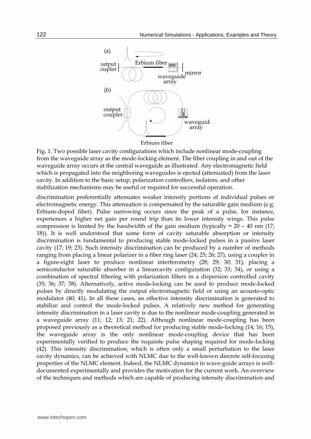

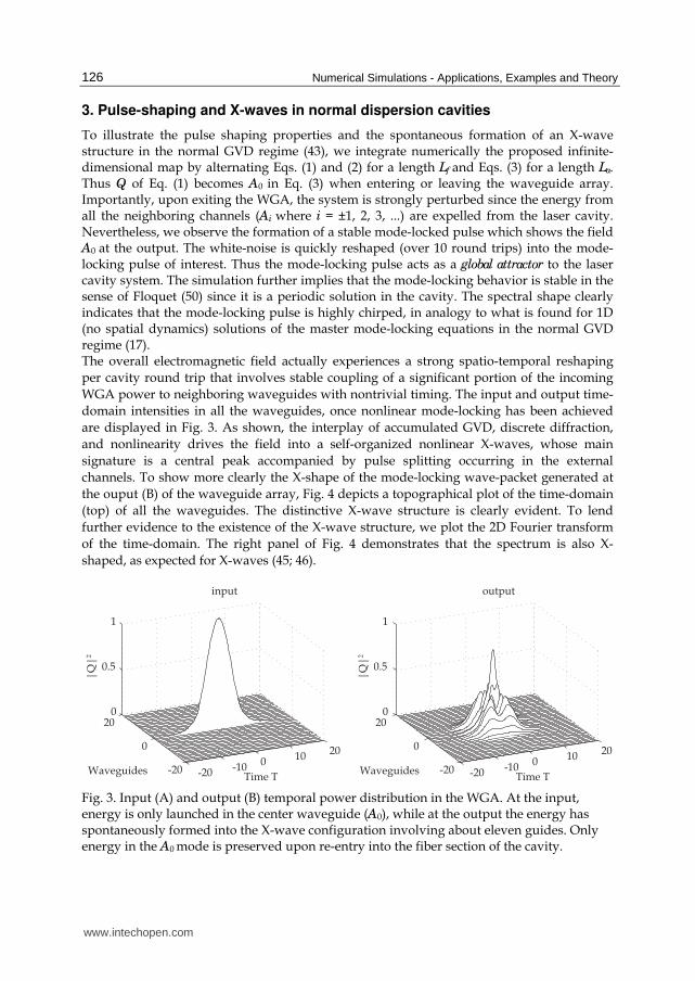


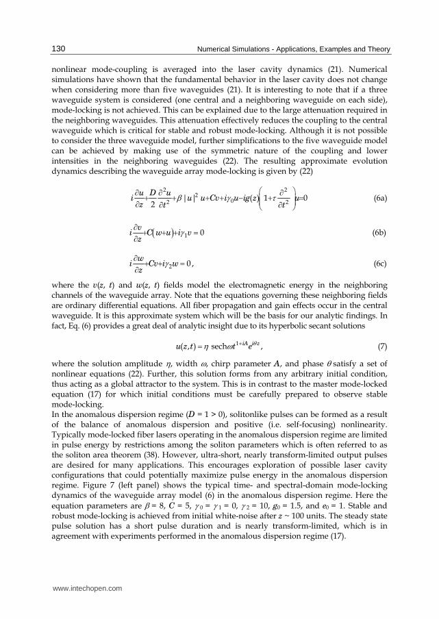


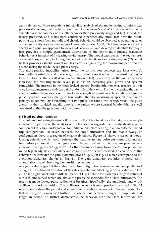


![Synthesis of waveguide antenna arrays using the coupling matrix … · 2017. 2. 17. · a rectangular waveguide operated at TE 10 mode (Taken from [31]) 23 Figure 2.15 Illustration](https://static.documents.pub/doc/80x56/6119a7cc0b5b53780d71cfc8/synthesis-of-waveguide-antenna-arrays-using-the-coupling-matrix-2017-2-17-a.jpg)

![Phase-Locking Josephson Junctions Arraysing.univaq.it/energeti/research/Fisica/jamapro12.pdf · junction-based systems such as multi-stacked junctions [5Š7], large planar arrays](https://static.documents.pub/doc/80x56/5ec5593513b08355f20aa454/phase-locking-josephson-junctions-junction-based-systems-such-as-multi-stacked-junctions.jpg)


